Bayes Factor Functions
Abstract
We describe Bayes factors functions based on z, t, , and F statistics and the prior distributions used to define alternative hypotheses. The non-local alternative prior distributions are centered on standardized effects, which index the Bayes factor function. The prior densities include a dispersion parameter that models the variation of effect sizes across replicated experiments. We examine the convergence rates of Bayes factor functions under true null and true alternative hypotheses. Several examples illustrate the application of the Bayes factor functions to replicated experimental designs and compare the conclusions from these analyses to other default Bayes factor methods.
Keywords: Bayes factor based on test statistic, default Bayes factor, Jeffreys prior, meta-analysis, non-local alternative prior density, normal-moment prior, replication study.
1 Introduction
Bayes factors provide a potentially useful alternative to P-values for summarizing outcomes of hypothesis tests. Unlike -values, Bayesian testing procedures quantify evidence that supports null hypotheses, and Bayes factors have a clear interpretation as the relative probability assigned by different hypotheses to data. Unfortunately, several factors hinder the practical application of Bayesian testing methodology. These factors include the specification of prior densities on the parameters implicit in each hypothesis and the prior probabilities on the hypotheses themselves. However, underlying concerns surrounding the construction of these tests are potentially even more problematic.
These concerns involve the basic definition of many Bayesian hypothesis tests (Tendeiro and Kiers, 2019). On the one hand, Bayesian tests frequently involve precise null hypotheses. Precise null hypotheses often represent a convenient approximation to the belief that an actual effect is “small” rather than identically 0. On the other, overly-dispersed prior distributions–often centered on the null hypotheses–are used to define alternative hypotheses. In the test of a normal mean , for example, Jeffrey-Zellner-Siow (JZS) priors impose Cauchy densities on a standardized effect, (e.g., Rouder et al., 2009). This Cauchy prior assigns one-half prior probability to standardized effects greater than 1.0 in magnitude and 0.3 probability to standardized effects greater than 2. However, in many areas of the social sciences, medicine, and biology, standardized effects greater than 1.0 are rarely encountered.
Resulting Bayes factors thus represent the relative evidence in support of idealized null hypotheses that exclude small effect sizes that are not scientifically important versus overly dispersed alternative hypotheses that assign a high probability to parameter values that are not scientifically plausible.
Related to these concerns, the dispersed priors used to define alternative hypotheses are usually local alternative priors densities that concentrate mass on parameter values that are consistent with null hypotheses. For instance, the modes of JZS priors (e.g., Rouder et al., 2009), intrinsic priors (e.g., Berger and Pericchi, 1996), and g-priors (e.g., Zellner, 1986) all occur at parameter values that define precise null hypotheses. Such local alternative priors weaken evidence in favor of true null hypotheses because data generated under null hypotheses also support alternative hypotheses. Indeed, local alternative hypotheses typically assign a higher probability to data generated from the null hypothesis than to data generated from the alternative.
With the advent of MCMC methodology, Bayes factors are now commonly used to choose between models containing high or very high dimensional parameter vectors. This practice requires the specification of high-dimensional prior densities, which amplifies the difficulties associated with specifying prior densities on scalar parameters. It also increases the sensitivity of Bayes factors to prior (and likelihood) misspecification.
Bayes factor functions (BFFs; Johnson et al. (2023)) were proposed to address these concerns.
In contrast to a single Bayes factor, BFFs express Bayes factors as a function of the prior densities used to define the alternative hypotheses. The prior densities are centered on standardized effects, which are used to index the BFF. By so doing, BFFs provide a summary of evidence in favor of alternative hypotheses corresponding to a range of scientifically interesting effect sizes.
As originally defined, BFFs are based on the sampling distributions of test statistics rather than the full data likelihood (Johnson, 2005). Under null hypotheses, the sampling distributions of these test statistics are known, and no prior specifications are required. Under common alternative hypotheses, the sampling distributions of the test statistics are determined by scalar non-centrality parameters. This dimension reduction simplifies the specification of prior densities under the alternative hypothesis. It also makes it straightforward to establish the connection between standardized effect sizes and the non-centrality parameters of the test statistics assumed under the alternative hypotheses.
To illustrate the construction of a BFF, consider a one-sided test. Suppose are i.i.d. , known, and define . Then where is the standardized effect (e.g., Cohen, 2013) and is the non-centrality parameter of the test statistic. Suppose further that the null hypothesis is and the alternative hypothesis is defined using a one-sided normal-moment prior density (Johnson and Rossell, 2010) as
The mode of this prior density is . By setting , the mode of the prior density occurs at , the non-centrality parameter of the test statistic. BFFs map standardized effects to Bayes factors defined from prior densities centered on non-centrality parameters that correspond to the given standardized effects. A plot of the BFF for and appears in Figure 1.
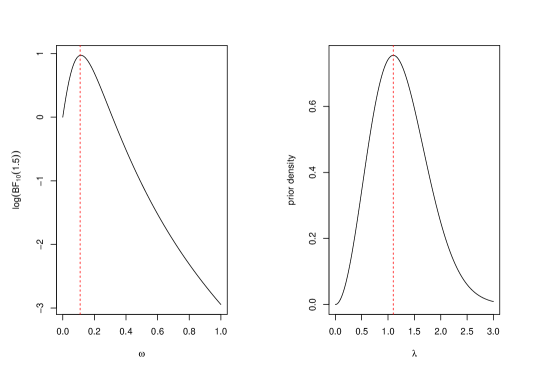
The BFF in Figure 1 shows support for the null hypothesis for priors centered on standardized effects . In contrast, the BFF exhibits support for alternative hypotheses corresponding to smaller standardized effects. For example, the logarithm of the Bayes factor corresponding to an alternative prior density centered on is 0.97. This feature of the BFF reflects the unfortunate reality that it is often not possible to rule out standardized effects less than in magnitude based on a sample size of .
By comparison, taking a standard Cauchy prior on the standardized effect results in a Bayes factor of 0.24 (), and taking a prior on (i.e., the intrinsic prior) yields a Bayes factor of 0.216 (). The BFF suggests that these levels of support for the null hypothesis are justified only when the prior density defining the alternative hypothesis is centered on standardized effect sizes greater than approximately 0.6 in magnitude.
Non-local prior densities play a central role in the definition of BFFs. Because non-local alternative priors have modes at non-null parameter values, they can be specified to assign a preponderance of their mass around non-null effects. They also assign negligible mass to effect sizes close to the null parameter value (Johnson and Rossell, 2010). This feature of non-local priors is particularly useful when precise null hypotheses only reflect a belief that an effect size is small.
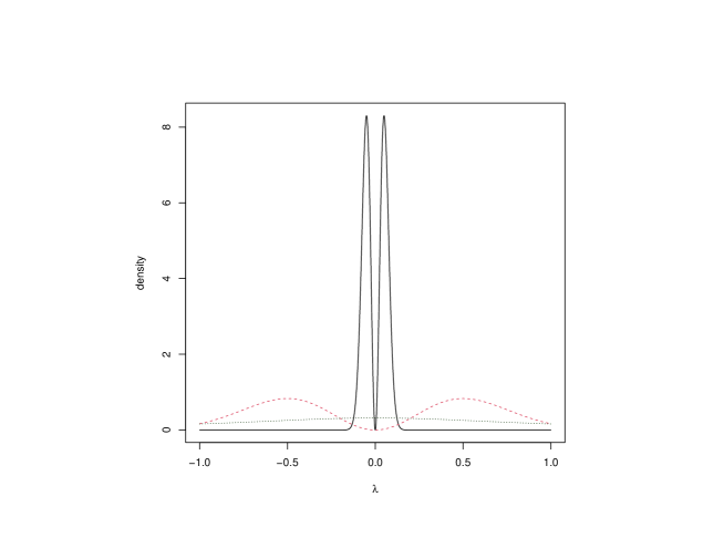
Concerning the latter point, one might assert that effect sizes under the alternative hypothesis are likely to concentrate near the null value. As Jeffreys stated, “the mere fact that it has been suggested that [an effect] is zero corresponds to some presumption that it is fairly small” (Jeffreys (1998), page 251). BFFs address this possibility by including Bayes factors obtained by centering the alternative hypothesis on small (but non-null) effect sizes. The values of BFFs at small effect sizes are thus larger than Bayes factors obtained using the default local prior specifications. This occurs because non-local priors centered on small effect sizes are sharply peaked, as illustrated in Figure 2. Thus, they provide more support to data generated from alternative models that are “close” to the null.
The BFFs defined in Johnson et al. (2023) were defined using one-parameter non-local alternative prior densities. That parameterization makes it possible to position the modes of prior densities at values corresponding to specified standardized effects. However, it does not provide additional flexibility for modeling the dispersion of test statistics collected in replicated experiments. In this article, we expand the class of non-local prior densities used to define BFFs to account for the dispersion of multiple test statistics collected in replicated designs.
We illustrate the application of this expanded framework to data collected in several experiments. These examples explore the potential information loss associated with using Bayes factors based on test statistics rather than fully parametric models. We also use data from replicated experiments to examine the potential loss of information associated with using “misspecified” priors. Finally, we describe a strategy for estimating the dispersion of the prior densities used in defining BFFs.
2 Bayes factors based on , , , and statistics
Following Johnson et al. (2023), let denote a normal distribution with mean and variance ; denote a distribution with degrees of freedom and non-centrality parameter ; a distribution on degrees of freedom and non-centrality parameter ; an distribution on degrees of freedom and non-centrality parameter ; a gamma distribution with shape parameter and rate parameter ; and a normal-moment distribution of order with mean and rate parameter (Johnson and Rossell, 2010). The density of the normal-moment random variable of order can be expressed
| (1) |
Normal-moment densities used in one-sided tests with positive non-centrality parameters are defined as
| (2) |
and similarly for . The modes of the above distributions occur at . As noted in Johnson and Rossell (2010) and discussed further in Pramanik and Johnson (2023) for and tests, these non-local priors accumulate evidence more quickly in favor of both true null and true alternative hypotheses for .
With these definitions in place, the following theorems describe the Bayes factors used in constructing BFFs based on standard test statistics. The interpretation of non-centrality parameters in these theorems appears in Section 4.
Theorem 2.1.
(Two-sided z-test) Assume the distributions of a random variable under the null and alternative hypotheses are described by
| (3) | |||||
| (4) |
Then the Bayes factor in favor of the alternative hypothesis is
| (5) |
where denotes the confluent hypergeometric function.
The proofs of all theorems are provided in the Supplemental Materials. The expression for the Bayes factor is valid for , but we have restricted the range to ensure that the prior density defining the alternative hypothesis is a non-local alternative. This restriction also guarantees that the prior density is differentiable at the origin.
Theorem 2.2.
(One-sided z-test) Assume the distributions of a random variable under the null and alternative hypotheses are described by
| (6) | |||||
| (7) |
Then the Bayes factor in favor of the alternative hypothesis is
| (8) |
where
| (9) |
Lemma 2.1.
- (i)
-
for some when is true ( in a one-sided test of ; in a one-sided test of ),
- (ii)
-
for some .
Then for some when applies, and when is true.
Theorem 2.3.
(Two-sided t-test) Assume the distributions of a random variable under the null and alternative hypotheses are described by
| (10) | |||||
| (11) |
Then the Bayes factor in favor of the alternative hypothesis is
| (12) | |||||
where
| (13) |
Here denotes the Gaussian hypergeometric function.
Theorem 2.4.
(One-sided t-test) Assume the distributions of a random variable under the null and alternative hypotheses are described by
| (14) | |||||
| (15) |
Then the Bayes factor in favor of the alternative hypothesis is
| (16) | |||||
where and are defined in (13).
Lemma 2.2.
In addition to the conditions of Theorem 2.3 and Theorem 2.4, suppose the following apply:
- (i)
-
for some when is true, ( in a one-sided test of ; in a one-sided test of ),
- (ii)
-
for some , and
- (iii)
-
for some .
Then for some when the alternative hypothesis is true and when the null hypothesis is true.
Theorem 2.5.
( test) Assume the distributions of a random variable under the null and alternative hypotheses are described by
| (17) | |||||
| (18) |
Then the Bayes factor in favor of the alternative hypothesis is
| (19) |
Lemma 2.3.
In addition to the conditions of Theorem 2.5, suppose the following hold:
- (i)
-
for some when the alternative hypothesis is true, and
- (iii)
-
for some .
Then for some when the alternative hypothesis is true and when the null hypothesis is true.
Theorem 2.6.
(F test) Assume the distributions of a random variable under the null and alternative hypotheses are described by
| (20) | |||||
| (21) |
Then the Bayes factor in favor of the alternative hypothesis is
| (22) |
Lemma 2.4.
In addition to the conditions of Theorem 2.6, suppose the following hold:
- (i)
-
for some when the alternative hypothesis is true, and
- (ii)
-
for some .
- (iii)
-
for some .
Then for some when the alternative hypothesis is true and when the null hypothesis is true.
3 Selection of prior hyperparameters
Bayes factors for common test statistics are described in Theorems 2.1-2.6. In each case, the Bayes factors depend on hyperparameters and that determine the shape and scale of the prior distributions that define the alternative hypotheses. To specify these hyperparameters, we begin by assuming that the value of is known.
Given , we set so that the mode of the prior distribution on the non-centrality parameter corresponds to a specified standardized effect size. To illustrate, consider a test of a null hypothesis based on a random sample , where and is unknown. For this test, , where is the usual unbiased estimate of . The distribution of is
| (23) |
where . Under the null hypothesis, . The non-centrality parameter of the distribution under the alternative hypothesis is , where is the standardized effect.
The prior distribution on from Theorem 2.3 is a normal moment prior, . The modes of this prior are . To define the BFF as a function of , we select so that the modes of the prior occur at . That is, we equate , which implies .
This approach for setting can be extended to more general settings by expressing the non-centrality parameter as a function of the standardized effect , say . In the example, . If denotes the prior density on given and , then for a given we define such that
| (24) |
the value of that makes the prior modes equal to .
Table 1 lists values of for several common statistical tests. This table generalizes relationships provided in Table 1 of Johnson et al. (2023) for the case .
The last three rows in Table 1 contain vectors of standardized effects . Because the recommended value of depends on only through the inner product , in many applications it is easier to study the BFF as a function of the root mean square effect size (RMSES) , defined as the square root of the mean of the squares of the components of ,
| (25) |
| Test | Statistic | Standardized Effect () | |
|---|---|---|---|
| 1-sample z | |||
| 1-sample t | |||
| 2-sample z | |||
| 2-sample t | |||
| Multinomial/Poisson | = | ||
| Linear model | = | ||
| Likelihood Ratio | = |
Given and , the theorems provided in Section 2 provide expressions for Bayes factors given a standardized effect and shape parameter . In principle, this allows us to construct a BFF by calculating Bayes factors as a function of both and , resulting in ordered triplets .
With only a single test statistic, it is generally not practical to estimate . With replicated data, however, it is possible to use the scale parameter to account for the variability in effect sizes between experimental replications. The next section describes the selection of .
4 Replicated data
Suppose that , represent test statistics collected from replicated experiments that test standardized effects centered on a common value . The non-centrality parameter for experiment is denoted by . Suppose that the are drawn independently from distributions , where are vectors of known constants and the data from each experiment are conditionally independent. In this setting, the Bayes factors obtained from individual experiments can be multiplied to obtain the BFF for the combined experiment. We aim to calculate the BFF as a function of when is not known a priori.
Several approaches might be taken toward performing this calculation. First, the value of might be fixed based either on subjective considerations or an estimate obtained from previous data. Alternatively, a prior distribution can be imposed on , and the BFF at each value of can be obtained by integrating over that prior density. Both of these approaches require subjective input. The approach taken here is to maximize the BFF with respect to , for each value of the standardized effect , to obtain the marginal maximum a posteriori (MMAP) estimate (see, for example, Doucet et al. (2002)). This strategy was previously advocated by Good (1967) and is similar to marginal maximum likelihood estimation as proposed in, for example, Bock and Aitkin (1981). It is also consistent with the recommendations of Dickey (1973), who suggested reporting Bayes factors for a range of hyperparameter values, and Albert (1990), who implemented the recommendations of both Good and Dickey in the specific context of contingency tables.
To illustrate the MMAP method, suppose that replicated experiments produce independent statistics on degrees-of-freedom based on observations. Under the alternative hypothesis, the non-centrality parameters of the statistics are assumed to be drawn independently from normal-moment priors with . Here, denotes the standardized effect size over the population of replicated experiments.
To obtain the MMAP estimate , we propose Jeffreys’ priors under the assumption that the non-centrality parameters are sampled independently from either normal-moment priors (Theorems 2.1-2.4) or gamma priors (Theorems 2.5–2.6).
For normal-moment prior densities with mode , the scale parameter satisfies . In the illustration above, for example, . Substituting this expression for and holding fixed, the Jeffreys’ prior for based on the assumption that are drawn independently from distributions is
| (26) |
where denotes the trigamma function. Using similar logic, the Jeffreys’ prior for based on the assumption that are drawn independently from distributions is
| (27) |
With these priors, the MMAP estimate can be defined as
| (28) |
where represents the marginal density of the test statistic , given and . Values of Bayes factors obtained using this criterion represent the maximum achievable Bayes factor from within the given class of prior densities having prior modes at .
When only a single replication of an experiment has been performed to test a hypothesis (i.e., ), the (unconstrained) BFF function evaluated at the maximum likelihood estimate of the standardized effect converges to the likelihood ratio statistic as . The use of Jeffreys priors as a constraint on in this setting avoids this phenomenon and guarantees that (see Section 6.2 of the Supplementary Material for further discussion of this issue.)
The restriction in (28) ensures that resulting non-local prior decreases at least quadratically in a neighborhood of the null value.
5 Applications
To illustrate the application of BFFs for replicated data, we re-analyzed several experimental datasets collected in the Many Labs projects (Ebersole et al., 2016, Klein et al., 2014). These projects studied the variation of psychological effects across replications of experiments conducted with different subject populations.
5.1 Stroop Task
The Many Labs 3 consortium replicated an experiment measuring the effect on response time for subjects performing the Stroop task (Ebersole et al., 2016). This effect is among the strongest and most widely replicated effects in experimental psychology. The Stroop task requires subjects to identify the color of the type of printed words. This task takes longer when there is discordance between the type’s color and the color’s name. For example, responding red takes longer than blue. After preprocessing the data to account for unusually long response times and incorrect answers (Greenwald et al., 2003), the authors “calculated the average response time for all correct responses separately for congruent and incongruent trials” and then “replaced response latencies for trials with errors using the mean of correct responses in that condition plus 600 ms.” They then “recomputed the means for congruent and incongruent trials overall” and used the difference between these two means divided by the standard deviation of all correct trials regardless of condition” to construct paired statistics. Table 2 depicts these statistics and their associated degrees of freedom across the 20 experimental sites that replicated this experiment.
| t | 9.38 | 9.85 | 7.36 | 11.62 | 7.85 | 12.56 | 11.01 | 10.15 | 13.52 | 10.14 |
|---|---|---|---|---|---|---|---|---|---|---|
| 8.90 | 10.37 | 11.68 | 9.11 | 16.97 | 8.82 | 8.46 | 5.93 | 12.17 | 9.37 | |
| df | 83 | 118 | 43 | 90 | 95 | 317 | 123 | 130 | 157 | 100 |
| 116 | 141 | 177 | 118 | 241 | 136 | 88 | 80 | 193 | 94 |
The null hypothesis in this study is that the mean difference in response times for the congruous and incongruous conditions is 0. Following the analyses presented in Ebersole et al. (2016), we assume that the statistics in Table 2 have standard distributions under the null hypothesis. Under the alternative hypothesis, we assume that the population mean difference in response times is and that the observational variance is , and let denote the standardized effect size. Given , we assume that the non-centrality parameters of the distributions of the statistics, say , are drawn independently from normal-moment distributions,
| (29) |
where from Table 1,
| (30) |
The Bayes factors based on the 20 experimental replications of the Stroop task, given , can be expressed as the product of Bayes factors from the individual experiments. Letting and applying Theorem 2.4,
| (31) |
For each value of , we determined by MMAP estimation, as described previously.
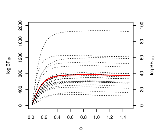
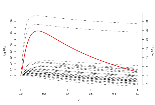
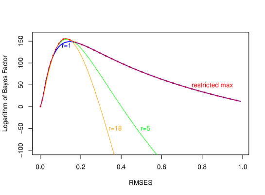
Figure 3 depicts the logarithm of the BFF obtained using these Bayes factors when is estimated using MMAP estimation (solid red line). Contributions from BFFs for individual studies are depicted as dashed lines (scale provided on the right). The MMAP estimate of the logarithm of the BFF, which also signifies the maximum evidence against the null, was 931.0274 at and . There is overwhelming evidence supporting alternative hypotheses corresponding to non-negligible effect sizes.
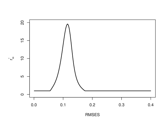
A plot of versus appears in Figure 4.
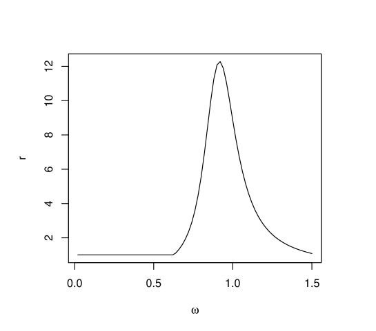
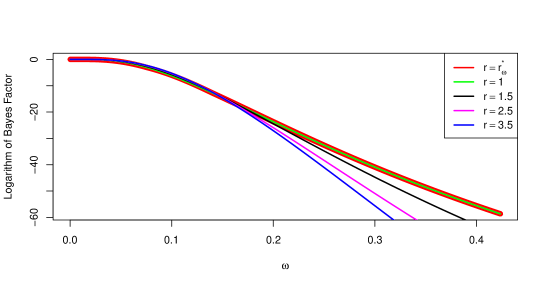
Figure 5 depicts BFFs for different values of . The green line represents the BFF for , and the red line denotes the BFF obtained corresponding to . This plot shows that while there is some gain in the maximum Bayes factor associated with using near the optimal value of , the default value of performs well across a wide range of standardized effects.
5.2 Persistence and Conscientiousness
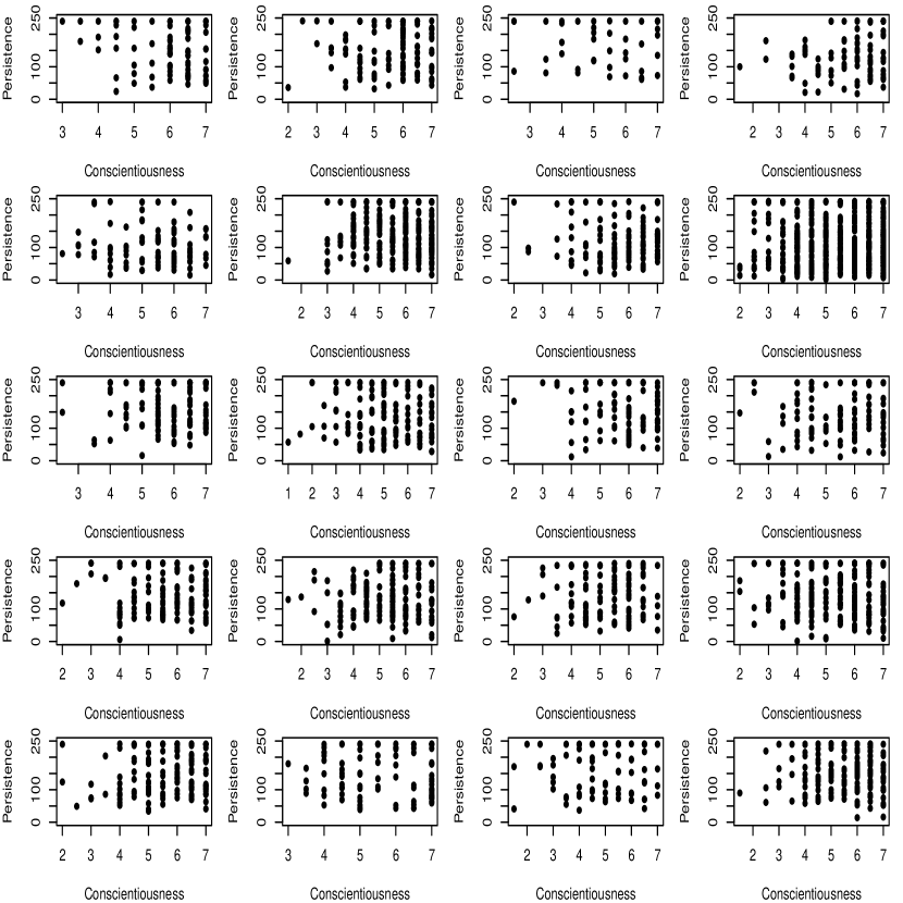
Another experiment replicated in the Many Labs 3 project examined the correlation between conscientiousness and persistence. Conscientiousness was measured using two items on the Ten Item Personality Inventory (TIPI; Gosling et al. (2003)) and persistence by the time participants spent solving anagrams, some of which were solvable and others not. The study performed in the Many Labs 3 project represented a modification of a study performed initially in De Fruyt et al. (2000). Table 3 provides the sample correlations and sample sizes collected in 20 replicated studies.
| r | -0.211 | 0.008 | -0.064 | 0.201 | -0.064 | 0.020 | -0.044 | 0.103 | -0.085 | -0.140 |
|---|---|---|---|---|---|---|---|---|---|---|
| 0.024 | 0.004 | 0.142 | 0.060 | -0.020 | 0.164 | -0.060 | -0.017 | -0.001 | 0.000 | |
| n | 84 | 117 | 42 | 90 | 96 | 314 | 126 | 131 | 156 | 101 |
| 118 | 139 | 179 | 117 | 240 | 137 | 89 | 80 | 177 | 95 |
The null hypothesis in this study is that there is no correlation between persistence and conscientiousness measures. To model the sample correlation coefficients obtained in each study, we rescaled Fisher’s z-transformation of the sample correlation coefficient Fisher (1915) and defined
| (32) |
Here, and denote the sample and population correlation coefficients for study population , . Let .
For large , we thus assume that
| (33) |
where
Under the null hypothesis, we assume . Under the alternative hypothesis, we define the standardized effect to be
| (34) |
where is the population correlation, and assume
| (35) |
This choice of places the modes of the prior distributions on the non-centrality parameters at .
Because the non-centrality parameters are assumed to be drawn independently from normal-moment prior densities and the replications of the experiments are assumed to be conditionally independent, it follows that the Bayes factors based on 20 replications of the experiment, given and , can be expressed as the product of Bayes factors from the individual experiments. Applying Theorem 2.2, it follows that the combined Bayes factors are
| (36) |
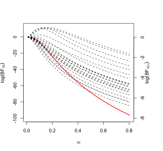
Figure 6 depicts the logarithm of the BFF obtained using these Bayes factors when is estimated using MMAP estimation (solid red line). Contributions from BFFs for individual studies are depicted as dashed lines (scale provided on the right). Based on data from all studies, this plot shows that there is very strong evidence for the null hypothesis (i.e., ) when alternative hypotheses are centered on , strong evidence (i.e., ) when , and positive evidence (i.e., ) when . Standardized effect sizes less than 0.20 are often considered small in the social sciences. Bayes factors in favor of alternative hypotheses centered on effect sizes greater than were less than . 111For small values of , . In particular, corresponds to .
For these data, for and did not exceed 1.172 in the interval . These values of reflect the substantial dispersion of sample correlations across studies.
In summary, these studies did not support a correlation between persistence, as defined using the anagram test, and conscientiousness, as measured by the TIPI.
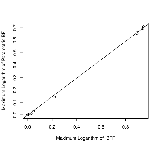
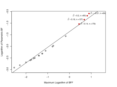
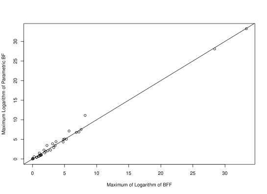
We next compared the BFF based on Fisher’s z transformation of the correlation coefficients with the fully parametric model proposed by Ly et al. (2016). In that model, conscientiousness (X) and persistence (Y) were assumed to follow a bivariate normal distribution with parameters . Under the null hypothesis, . Under the alternative hypothesis, the prior on was a stretched-beta () prior. Non-informative priors were assumed on under both null and alternative models (as detailed in Section 4.2.2 of Ly et al. (2016)). The results of this comparison are presented in Figures 7 and 8.
Figure 7 demonstrates a strong correlation between the maximum Bayes factor based on test statistics and the stretched-beta model. Maximization for the BFF was performed with respect to and for the stretched-beta model with respect to . The maximum logarithm of the Bayes factors using either method is non-negative because the null hypothesis can be obtained as an extreme limit of either or .
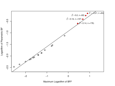
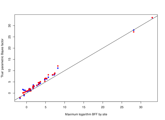
Figure 8 compares evidence in support of the null hypothesis when the BFF is restricted to standardized effect sizes greater than 0.2 (as suggested in Pramanik and Johnson (2023)) and the parametric model when either a stretched-Jeffreys or uniform prior is imposed on . This figure shows a high correlation between the two Bayes factors. The BFF provides more evidence than the parametric model in favor of alternative hypotheses for the four studies with the highest correlations (), and approximately the same or slightly less evidence in favor of the null hypothesis when the sample correlations were close to 0.
In this example, there was substantial dispersion in the values of the sample correlation coefficients between studies. For this reason, larger values of were not favored, and or close to one yielded the maximum Bayes factor for most values of . A plot of BFFs for various values of is provided in Figure 9.
5.3 Low-vs.-high category scales
In an experiment replicated in the Many Labs 1 project (Klein et al., 2014), subjects at 36 experimental sites were divided into two groups. At each site, participants reported how much time they spent watching television each day. One group responded on a high-frequency instrument, where response options ranged from “up to half an hour per day” to more than “two and a half hours per day.” The low-frequency group’s responses ranged from “less than two and a half hours” to “more than four and a half hours” a day (Schwarz et al., 1985). To test the hypothesis that reporting scale affected responses, the authors of Klein et al. (2014) constructed a single contingency table in which rows corresponded to the experimental group and columns to less than or greater than 2.5 hours of television time. They pooled data across the 36 performance sites, which included 5,899 subjects, and reported a highly significant chi-squared value of 324.4 on 1 degree of freedom.
As a first step in analyzing these data, we computed the logarithm of the BFF based on 36 chi-squared statistics calculated at each experimental site after fixing . Figure 10 depicts the resulting BFF curves for the individual sites. Also displayed in this plot is the logarithm of the BFF obtained by combining information at all sites. These curves show substantial consistency in the optimal RMSES across sites, with maxima typically occurring near 0.13.
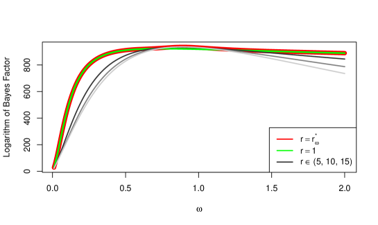
Next, we applied (28) to maximize the BFF at each value of with respect to . The maximum logarithm of this curve, displayed in Figure 11, was 155.9 at for . Also displayed are the logarithms of the BFFs corresponding to . The maximum of the logarithm of the BFF for was 148.7 at . A plot of versus appears in Figure 12.
This analysis demonstrates that more evidence can be obtained for true alternative hypotheses when less dispersed priors are imposed on the non-centrality parameters of the test statistic, provided the standardized effect sizes are consistent across replications.
We next investigated the potential information loss incurred by computing BFFs based on test statistics rather than a fully parametric default Bayesian model. To this end, we compared our BFFs to the parametric model described in Albert (1990). Albert defined Bayes factors for contingency tables by modeling the cell probabilities under alternative hypotheses as mixtures of Dirichlet priors centered on an independent surface. Under null hypotheses, the cell probabilities were expressed as a product of independent Dirichlet densities on the marginal row () and column () probabilities. The resulting priors on cell probability vectors were
| (37) |
where denotes an -dimensional Dirichlet density with parameter . Albert recommended , but also considered . The parameter determines the concentration of the prior around the independence surface; the independence prior for the null hypothesis corresponds to . The alternative priors defined by this specification are local alternative prior densities because they are non-zero at values consistent with the null hypothesis of independence.
Because serves a similar function as in the BFF framework, we compared the maximum of Albert’s Bayes factors for each of the 36 contingency tables to the maximum of the BFF, after maximizing over and . The results of the comparison appear in Figure 13. This figure shows a high correlation () between the Bayes factors based on test statistics and the multinomial-Dirichlet model. We note that the computation of each parametric Bayes factor requires the numerical evaluation of a two-dimensional integral for each value of .
The maximum logarithm of the Bayes factors displayed in Figure 13 is, by definition, non-negative because neither nor were restricted to prevent the alternative model space from including the null model of independence.
The availability of replicated data in this example also allowed us to investigate the performance of BFFs to Bayes factors calculated from empirical estimates of prior distributions on the cell probabilities. We performed this comparison by specifying hierarchical models on the cell probabilities for individual tables. We used data from 35 contingency tables to estimate parameters in the hierarchical model. The posterior distributions on these parameters were used to approximate the prior distribution on the cell probabilities for the excluded table. We repeated this procedure for each contingency table using the remaining tables to train the hierarchical model.
We considered two hierarchical models for the cell probabilities. In the larger model, we assumed that the cell probabilities for the low-frequency and high-frequency groups at each experimental site were drawn from independent beta distributions with parameters (low-frequency group) and (high-frequency group).
We also posited a bivariate beta model for the low- and high-frequency cell probabilities. Letting , , and denote independent standard gamma random variables with shape parameters , , and , the probability of success (i.e., greater than 2.5 hours) for the low-frequency group and high-frequency groups at a given site were assumed to be
| (38) |
respectively. This model enforces a positive correlation between the cell probabilities at each site. (Further details on the bivariate beta model are described in Olkin and Liu (2003).) We assumed independent standard half-Cauchy distributions on and to complete the model specification.
Figure 14 depicts the relation between the Bayes factors obtained by training the independent beta models and bivariate beta models against the maximum of the BFF at each experimental site. The slopes of the least squares line obtained by regressing the logarithm of the empirical Bayes factors on the maximum of the logarithm of the BFF were 0.99 for both trained models, and the intercepts were 1.00 (bivariate beta) and 1.09 (independent beta) models. In this case, the penalty for using the BFF based on test statistics rather than a more accurate, empirically estimated prior model is approximately one unit on the logarithmic scale. Not surprisingly, the BFF function in Fig. 12–based on data from all sites–provides much more convincing evidence for the alternative hypotheses than any single Bayes factors obtained by using 35 sites to estimate a prior density for the remaining site.
As an aside, it is worth contrasting this method for estimating the empirical prior density on hyperparameters to the approach sometimes used with intrinsic prior and fractional Bayes factor methodology. In the latter cases, a single data set generated from a density indexed by a single draw from a prior distribution is (conceptually) resampled to estimate a prior density. In the preceding analysis, replicated data generated from 35 distinct densities, each reflecting an independent parameter value drawn from a prior density, were used to estimate the hyperparameters of that prior density.
6 Discussion
Bayes factor functions based on test statistics present compelling advantages over standard methods for calculating Bayes factors. They eliminate the computational challenges that arise when Bayes factors are computed from complex statistical models and reduce subjectivity when defining prior distributions on model parameters. By indexing Bayes factors according to standardized effects, BFFs simplify the aggregation of evidence across replicated studies. In the examples considered in Section 5, BFFs provided results comparable to fully parametric models despite being easier to define and compute.
The decision to base Bayes factors on test statistics rather than complete probability models has advantages and disadvantages. The final example illustrates that fully specified joint probability models can produce more informative Bayes factors than default BFFs. However, informative prior distributions derived from previous replications of similar experiments or other subjective sources are not always available. In addition, the actual distribution of a test statistic may more closely approximate its nominal distribution than the assumed distribution for raw data.
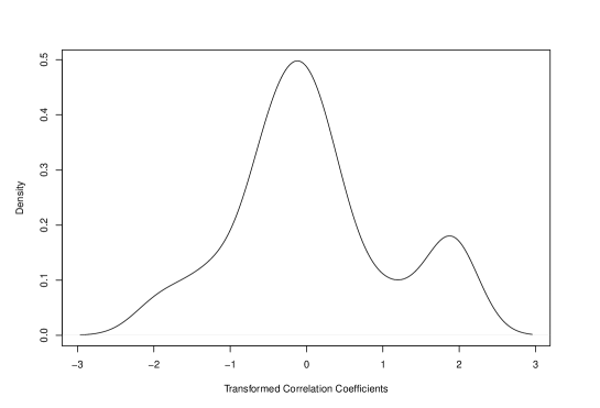
To illustrate the latter point, consider again the data from Section 5.2 concerning the correlation between persistence and conscientiousness. Figure 15 depicts scatter plots of the data collected at the 20 experimental sites. Arguably, these data are not distributed according to bivariate normal distributions. For comparison, Figure 16 depicts a default density estimate of the z-transformed correlation coefficients. This figure suggests that the sample correlation coefficients are also not normally distributed. However, approximating these data by a mixture of normal densities may be more realistic than approximating the original data distribution by mixtures of bivariate normal distributions.
Finally, the examples demonstrate that generalizing the class of probability distributions used to model the non-centrality parameters of test statistics in Theorems 2.1 - 2.6 can increase the evidence collected in favor of true alternative hypotheses. This effect is most beneficial when combining evidence across replicated experiments that report consistent findings. For hypothesis tests based on single experiments or for experiments in which the null hypothesis is favored, BFFs calculated using a default value of were very similar to BFFs calculated after maximizing over .
The BFF package (https://CRAN.R-project.org/package=BFF) available on CRAN computes the expressions of BFFs and the combined BFFs stated in Theorems 2.1 - 2.6.
Acknowledgment
The authors acknowledge support from the National Science Foundation, NSF DMS 2311005.
References
- Albert (1990) J. Albert. A Bayes test for a two-way contingency table using independence priors. The Canadian Journal of Statistics, 18:347–363, 1990.
- Berger and Pericchi (1996) J. O. Berger and L. R. Pericchi. The intrinsic bayes factor for model selection and prediction. Journal of the American Statistical Association, vol. 91, 1996. doi: https://doi.org/10.2307/2291387.
- Bock and Aitkin (1981) R. Bock and M. Aitkin. Maximum marginal likelihood estimation of item parameters: Application of an EM algorithm. Psychometrika, 46:443–459, 1981.
- Cohen (2013) J. Cohen. Statistical power analysis for the behavioral sciences. Academic press, 2013.
- De Fruyt et al. (2000) F. De Fruyt, L. Van de Wiele, and C. Van Heeringen. Cloninger’s psychobiological model of temperament and character and the five-factor model of personality. Personality and individual differences, 29(3):441–452, 2000.
- Dickey (1973) J. Dickey. Scientific reporting. Journal of the Royal Statistical Society, Series B, 35:285–305, 1973.
- Doucet et al. (2002) A. Doucet, S. Godsill, and C. Robert. Marginal maximum a posteriori estimation using Markov chain Monte Carlo. Statistics and Computing, 12:77–84, 2002.
- Ebersole et al. (2016) C. R. Ebersole, O. E. Atherton, A. L. Belanger, H. M. Skulborstad, J. M. Allen, J. B. Banks, E. Baranski, M. J. Bernstein, D. B. Bonfiglio, L. Boucher, E. R. Brown, N. I. Budiman, A. H. Cairo, C. A. Capaldi, C. R. Chartier, J. M. Chung, D. C. Cicero, J. A. Coleman, J. G. Conway, W. E. Davis, T. Devos, M. M. Fletcher, K. German, J. E. Grahe, A. D. Hermann, J. A. Hicks, N. Honeycutt, B. Humphrey, M. Janus, D. J. Johnson, J. A. Joy-Gaba, H. Juzeler, A. Keres, D. Kinney, J. Kirshenbaum, R. A. Klein, R. E. Lucas, C. J. Lustgraaf, D. Martin, M. Menon, M. Metzger, J. M. Moloney, P. J. Morse, R. Prislin, T. Razza, D. E. Re, N. O. Rule, D. F. Sacco, K. Sauerberger, E. Shrider, M. Shultz, C. Siemsen, K. Sobocko, R. Weylin Sternglanz, A. Summerville, K. O. Tskhay, Z. van Allen, L. A. Vaughn, R. J. Walker, A. Weinberg, J. P. Wilson, J. H. Wirth, J. Wortman, and B. A. Nosek. Many labs 3: Evaluating participant pool quality across the academic semester via replication. Journal of Experimental Social Psychology, 67:68–82, 2016. ISSN 0022-1031. doi: https://doi.org/10.1016/j.jesp.2015.10.012. URL https://www.sciencedirect.com/science/article/pii/S0022103115300123. Special Issue: Confirmatory.
- Fisher (1915) R. Fisher. Frequency distribution of the values of the correlation coefficient in samples of an indefinitely large population. Biometrika, 1915. doi: 10.2307/2331838.
- Good (1967) I. Good. A bayesian significance test for multinomial distributions. Journal of the Royal Statistical Society, Series B, 29:399–431, 1967.
- Gosling et al. (2003) S. D. Gosling, P. J. Rentfrow, and J. Swann, W. B. A very brief measure of the big-five personality domains. Journal of Research in Personality, 2003. doi: https://doi.org/10.1016/S0092-6566(03)00046-1.
- Greenwald et al. (2003) A. Greenwald, B. Nosek, and M. Banaji. Understanding and using the implicit association test: I. an improved scoring algorithm. J Pers Soc Psychol, 2003. doi: 10.1037/0022-3514.85.2.197.
- Johnson (2005) V. E. Johnson. Bayes factors based on test statistics. Journal of the Royal Statistical Society. Series B (Statistical Methodology), 67(5):689–701, 2005. ISSN 13697412, 14679868. URL http://www.jstor.org/stable/3647614.
- Johnson and Rossell (2010) V. E. Johnson and D. Rossell. On the use of non-local prior densities in bayesian hypothesis tests. Journal of the Royal Statistical Society. Series B (Statistical Methodology), 72(2):143–170, 2010. ISSN 13697412, 14679868. URL http://www.jstor.org/stable/40541581.
- Johnson et al. (2023) V. E. Johnson, S. Pramanik, and R. Shudde. Bayes factor functions for reporting outcomes of hypothesis tests. Proceedings of the National Academy of Sciences, 2023. URL https://doi.org/10.48550/arXiv.2210.00049.
- Klein et al. (2014) R. A. Klein, K. Ratliff, M. Vianello, J. Reginald B. Adams, S. Bahník, M. J. Bernstein, K. Bocian, M. Brandt, B. Brooks, C. Brumbaugh, Z. Cemalcila, J. J. Chandler, W. Cheong, W. E. Davis, T. Devos, M. Eisner, N. Frankowska, D. Furrow, E. M. Galliani, F. Hasselman, J. A. Hicks, J. F. Hovermale, S. J. Hunt, J. R. Huntsinger, H. IJzerman, M.-S. John, J. Joy-Gaba, H. Kappes, L. E. Krueger, J. Kurtz, C. Levitan, R. Mallett, W. Morris, A. J. Nelson, J. A. Nier, G. Packard, R. Pilati, A. M. Rutchick, K. Schmidt, J. Skorinko, R. W. Smith, T. G. Steiner, J. Storbeck, L. van Swol, D. Thompson, A. van’t Veer, L. A. Vaughn, M. A. Vranka, A. Wichman, J. A. Woodzicka, and B. A. Nosek. Investigating variation in replicability: A “many labs” replication project. Social Psychology, 45:142–152, 2014. doi: https://doi.org/10.1027/1864-9335/a000178.
- Ly et al. (2016) A. Ly, J. Verhagen, and E.-J. Wagenmakers. Harold jeffreys’s default bayes factor hypothesis tests: Explanation, extension, and application in psychology. Journal of Mathematical Psychology, 72:19–32, 2016. ISSN 0022-2496. doi: https://doi.org/10.1016/j.jmp.2015.06.004. URL https://www.sciencedirect.com/science/article/pii/S0022249615000383. Bayes Factors for Testing Hypotheses in Psychological Research: Practical Relevance and New Developments.
- Olkin and Liu (2003) I. Olkin and R. Liu. A bivariate beta distribution. Statistics and Probability Letters, 62:407–412, 2003.
- Pramanik and Johnson (2023) S. Pramanik and V. Johnson. Efficient alternatives for bayesian hypothesis tests in psychology. Psychological Methods, 2023. URL https://doi.org/10.1037/met0000482.
- Rouder et al. (2009) J. Rouder, P. Speckman, D. Sun, and R. Morey. Bayesian t tests for accepting and rejecting the null hypothesis. Psychonomic Bulletin & Review, 16:225–237, 2009. doi: 10.3758/PBR.16.2.225.
- Schwarz et al. (1985) N. Schwarz, H. Hippler, B. Deutsch, and F. Strack. Response scales: Effects of category range on reported behavior and comparative judgments. Public Opinion Quarterly, 49:338–395, 1985.
- Tendeiro and Kiers (2019) J. Tendeiro and H. A. L. Kiers. A review of issues about null hypothesis bayesian testing. Psychological Methods, 2019. doi: 10.1037/met0000221. URL https://doi.org/10.1037/met0000221.
- Winkelbauer (2014-07-15) A. Winkelbauer. Moments and absolute moments of the normal distribution. arXiv, 2014-07-15. URL https://doi.org/10.48550/arXiv.1209.4340.
- Zellner (1986) A. Zellner. On Assessing Prior Distributions and Bayesian Regression Analysis with g Prior Distributions. Bayesian Inference and Decision Techniques: Essays in Honor of Bruno de Finetti. Studies in Bayesian Econometrics and Statistics. Vol. 6. New York: Elsevier, 1986. ISBN 78-0-444-87712-3.
Supplementary Material
6.1 Proofs of theorems and lemmas
Theorem 2.1.
The density of under the null is given by
| (39) |
Under the alternative, the density of is,
| (40) |
Assuming that the density of takes the form given by equation (2), the marginal density under the alternative is
| (41) |
Let , and note that
Using the expression for absolute fractional moments given in Winkelbauer (2014-07-15), equation (41) leads to
| (42) | |||||
Dividing equation (42) by equation (39) yields the expression of the BFF in Theorem 2.1.
∎
Theorem 2.3.
When the alternative is true, the marginal distribution of the test statistic is
| (45) |
Let,
| (46) | |||||
Assuming ,
| (47) | |||||
Substituting in (6.1), the marginal density is
| (48) |
Hence the Bayes factor function based on two sided statistic is
| (49) |
∎
Lemma 2.2.
Re-write as
It is known that . Let
,
When the alternative is true, are . As , the Bayes factor in favour of the alternative can be approximated as
This implies
When the null is true, and are .
∎
Theorem 2.4 and Theorem 2.2.
Under the null, the probability density function of is
The probability density function of a non-central t-distribution can be expressed using a power series expansion of the confluent hypergeometric function as
| (51) | |||||
where .
Define
| (52) |
and
| (53) |
Combining equations (51), (6.1) and (6.1), the Bayes factor in favor of the alternative based on a one-sided t-test statistic is given by
| (54) |
Define
Then
Note that and as , .
Hence, as ,
For large , . Hence, . This implies
Thus the Bayes factor function in favour of the alternative hypothesis based on a one-sided -test statistic is
| (55) | |||||
∎
Theorem 2.5.
Under the null hypothesis, the density of is
| (56) |
and under the alternative hypothesis is
This density can be simplified as
Theorem 2.6.
Under the null hypothesis, the density of is
| (60) |
Under the alternative hypothesis, the marginal density of is
6.2 Maximization of for
We now examine the MMAP of when Bayes factors are computed from a single test statistic according to the assumptions described in Sections 2-4. We assume that a non-informative prior (either (26) or (27)) is imposed on and that is constrained to be greater than or equal to 1. Under these assumptions, we show that .
Letting denote one of the four test statistics considered in Section 2, the marginal density of under the alternative, for a given value of , can be expressed as
To prove our claim it is enough to show that
| (62) |
6.3 Case 1: Normal Moment Prior for and Jeffrey’s Prior for
For normal moment prior densities and the Jeffreys prior on , we have
Note that . Differentiating with respect to gives
| (63) |
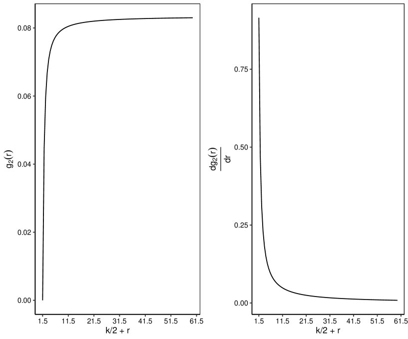
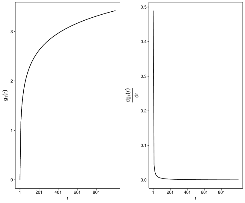
This derivative is difficult to study analytically due to its dependence on polygamma functions. However, a plot of and its derivative is depicted in Figure 17. These plots show that is an increasing function of with a positive slope. It can further be shown that as . For large , and . This implies,
| (64) | |||||
This suggests that and that the MMAP of is 1.
6.4 Case 2: Non-local Gamma Prior for and Jeffrey’s Prior for
Denote the LHS of equation (62) as,
Taking logarithms on both sides,
Note that . Differentiating both sides with respect to ,
Like above, is difficult to study analytically. However, Figure 18 suggests that this function is strictly positive as a function of , ( and ) again suggesting that the MMAP of is 1. The assertion gains additional support from the observation that tends towards zero as approaches infinity. Using the recursive relation and asymptotic expansion of polygamma functions,
| (66) | |||||