Homogeneous control design using invariant ellipsoid method

Abstract

The invariant ellipsoid method is aimed at minimization of the smallest invariant and attractive set of a linear control system operating under bounded external disturbances. This paper extends this technique to a class of the so-called generalized homogeneous system by defining the $\mathbf{d}-$homogeneous invariant/attractive ellipsoid. The generalized homogeneous optimal (in the sense of invariant ellipsoid) controller allows further improvement of the control system providing a faster convergence and better precision. Theoretical results are supported by numerical simulations and experiments.

I Introduction

During the formulation of any control issue, there is always a discrepancy between the actual system and the mathematical model used for control design. This mismatch comes from the unmodelled dynamics, uncertainties in system parameters or the approximation of complex plant. However, the engineer needs to guarantee that the designed controller is able to achieve the required performance despite of all these mismatches. This leads to the development of the so-called robust control methods solving this problem. Robust control design is an approach dealing with perturbations of a nominal system. Its objective is to attain the certain level of performance or stability in the system despite the presence of bounded disturbance. Several well-known methodologies of robust control design have been invented such as sliding mode control, $H_{\infty}$ approach, attractive/invariant ellipsoid method, and so on. The sliding mode control (SMC) as a robust control design methodology is known since 1960s in Russia. The first survey paper by V. Utkin is published in English in 1977 [1]. Sliding mode methodology has been devised for both linear and nonlinear system [2], [3] and delivers a good performance in numerous real-world scenarios [4]. The concepts of the $H_{\infty}$ control theory to solve the robust stabilization problem for linear system can be found in [5, 6, 7]. Later the $H_{\infty}$ control methodology was extended to the various systems [8].

The basic ideas of the attractive/invariant method were introduced in the papers [9, 10, 11]. One of the main features of this method is that the states of the robustly stabilized system converge to a minimal (in some sense) ellipsoidal set regardless of perturbations or uncertainties satisfying certain bounds. The attractive/invariant ellipsoid method is widely applied to various control and estimation problems for both linear [12] and nonlinear plants [13]. The key feature of the method is by using Linear Matrix Inequalities (LMIs) for control parameters tuning [14]. For instance, the problem of suppressing bounded additive external disturbance in terms of the invariant ellipsoid is studied in [12] for linear plant. It turns out to be equivalent to a Semi-Definite Programming (SDP) problem minimizing the invariant ellipsoid of the closed-loop linear system to design the optimal robust feedback. The further suppression of bounded external disturbance beyond a certain level using the same linear feedback strategy seems infeasible. The purpose of this paper is to extend the attractive/invariant ellipsoid technique to a class of controller known as generalized homogeneous controllers [15], which may provide a better quality of control such as faster convergence, better robustness and smaller overshoots.

A symmetry with respect to a dilation is referred to as homogeneity [16], [17]. This concept is applied in the field of control theory and experiment for the purpose of system analysis, controller and observer design (e.g. [18, 19, 20, 21, 22, 23, 24] and references therein). The standard (Euler) homogeneity means that a function $f(x)$ remains invariant with respect to the scaling of its argument $f(e^{s}x)=e^{\nu s}f(x),\forall s,x\in\mathbb{R}$, where the constant $\nu$ is called the homogeneity degree. The generalized (weighted) dilation of vector $x=(x_{1},x_{2},..,x_{n})^{\top}\in\mathbb{R}^{n}$ is introduced by V.I. Zubov in 1958 [16]: $(x_{1},x_{2},..,x_{n})\to(e^{r_{1}s}x_{1},e^{r_{2}s}x_{2},...,e^{r_{n}s}x_{n}),s\in\mathbb{R}$, where the positive numbers $r_{1},r_{2},...,r_{n}$ are the weights specifying the dilation rate of each coordinate. Nonlinear (geometric) dilutions are studied in [25], [26], [27]. This paper deals with the linear geometric dilation [28] given by $x\to e^{G_{\mathbf{d}}s}x$, where $G_{\mathbf{d}}\in\mathbb{R}^{n\times n}$ is anti-Hurwitz matrix. The homogeneity as a relaxation of linearity can provide an extra degree of freedom for further minimization of the disturbance effects [29].

The key contribution of this article is the extension of the attractive/invariant ellipsoid approach to a category of generalized homogeneous control systems[30]. Specifically, we present the concept of a homogeneous invariant ellipsoid through the use of the canonical homogeneous norm [28] and derive its characterization in terms of LMIs. We also show that an optimal homogeneous control design is obtained by solving an SDP problem minimizing the homogeneous attractive/invariant ellipsoid of the system. As an example, the controlled rotary inverted pendulum is studied, where it demonstrate that the optimal (in the sens of attractive ellipsoid) homogeneous controller can stabilize the pendulum with a better precision than the optimal (in the same sense) linear controller without any degradation of the control signal quality.

The structure of paper is as follows: The problem statement is outlined in Section II. Section III delves into the concept of homogeneous theories. The main results about the conditions of being a $\mathbf{d}$-homogeneous attractive/invariant ellipsoid and the optimal homogeneous controller design are explained in Section IV and Section V. The last Section VI provides the simulation results to support the proposed theories.

Notation : $\mathbb{R}$: set of real numbers, $\mathbb{R}_{+}=\{x\in\mathbb{R}:x>0\}$; $\|x\|=\sqrt{x^{\top}x}$: norm in $\mathbb{R}^{n}$; $\|x\|_{P}=\sqrt{x^{\top}Px}$: weight norm in $\mathbb{R}^{n}$; $\mathrm{diag}\{\lambda_{i}\}_{i=1}^{n}$ : the diagonal matrix with elements $\lambda_{i}$; $P\succ 0(\prec 0,\succeq 0,\preceq 0)$ for $P\in\mathbb{R}^{n\times n}$ means that the matrix $P$ is symmetric and positive (negative) definite (semi definite); $\lambda_{min}(P)$ and $\lambda_{max}(P)$ : the minimal and maximal eigenvalues of matrix $P=P^{\top}$; for $P\succeq 0$ the square root of $P$ is a matrix $M=P^{\frac{1}{2}}$ such that $M^{2}=P$; $\mathrm{tr}(P)$ : trace of matrix $P$; if $V:\mathbb{R}^{n}\mapsto[0,+\infty)$ is a positive definite function and $\dot{x}=f(t,x)$ is an ODE with $f$ continuous on $c$ then we denote the time derivative of $V$ along all solutions of the ODE as $\frac{d}{dt}V(x):=\frac{\partial V}{\partial x}f(t,x);$ a function $\gamma:\mathbb{R}_{\geq 0}\to\mathbb{R}_{\geq 0}$ is said to be of class $\mathcal{K}$ if it is continuous strictly increasing and satisfies $\gamma(0)=0$; a function $\beta:\mathbb{R}_{\geq 0}\times\mathbb{R}_{\geq 0}\to\mathbb{R}_{\geq 0}$ is said to be of class $\mathcal{KL}$ if for each fixed $t$ the mapping $\beta(\cdot,t)$ is of class $\mathcal{K}$ and for each fixed $s$ it is decreasing to zero on t as $t\to\infty$; $L^{\infty}$ is the space of Lebesgue measurable essentially bounded function $\sigma:\mathbb{R}_{+}\to\mathbb{R}^{n}$ with norm defined as $\|\sigma\|_{L^{\infty}}:=\mathrm{ess}\sup_{t\in\mathbb{R}_{+}}\|\sigma(t)\|_{\infty}<+\infty$; $1_{n}\in\mathbb{R}^{n}$ is a vector with all element is 1

II Problem statement

In this paper, we deal with the linear time-invariant system with additive perturbations,

$$\dot{x}(t)=Ax(t)+Bu(t)+D\omega(t),\quad t>0$$ (1)

where $x(t)\in\mathbb{R}^{n}$ is the system state, $\omega(t)\in\mathbb{R}^{p}$ is an external bounded disturbance, $u(t)\in\mathbb{R}^{m}$ is the control input, $A\in\mathbb{R}^{n\times n}$ is nilpotent, $B\in\mathbb{R}^{n\times m}$, $D\in\mathbb{R}^{n\times p}$ are constant matrix. We assume that the pair $\{A,B\}$ is controllable.

We study the feedback stabilization problem of the system (1) with perturbations. In the general case, it is not possible to achieve a precise stabilization of this system to a zero state, hence a feedback controller $u(x)$ needs to be optimized in order to minimize (in some sense) the effect of external disturbance $\omega$. For the case of a linear stabilizing feedback there are several well-known methodologies tackling this problem. For example, $H_{\infty}$ and $H_{2}$ algorithms (see e.g., [31, 32]) suggest to optimize a norm of a transfer function, while the attractive/invariant ellipsoid method [12, 13] optimizes (in a certain sense) the attractive/invariant set of the system (1) with a linear feedback. This paper is aimed at an extension of the latter approach to a special class of generalized homogeneous [33, 28, 30, 23] feedback laws. The mentioned nonlinear control algorithms are known to be efficient for finite/fixed-time stabilization of linear plants. Our objective is to design a generalized homogeneous controller that minimizes the attractive/invariant ellipsoid of the closed-loop system (1) with

$$\omega^{\top}\!(t)Q\omega(t)\leq 1,\quad\omega\in L^{\infty}(\mathbb{R}_{+},\mathbb{R}^{p}),$$ (2)

where $0\prec Q=Q^{\top}\in\mathbb{R}^{p\times p}$ is a known matrix.

III Preliminaries: Elements of the Homogeneity Theory

III-A Linear dilation and monotonicity

The homogeneity is a symmetry of an object (e.g. a function or a set) with respect to a group of transformations called dilation. In this paper we deal only with the so-called linear dilation[15]: $x\mapsto\mathbf{d}(s)x,x\in\mathbb{R}^{n},s\in\mathbb{R}$, where $s\in\mathbb{R}$ is a parameter of the dilation and

$$\mathbf{d}(s)=e^{sG_{\mathbf{d}}}=\sum_{i=0}^{+\infty}\frac{s^{i}G_{\mathbf{d}}^{i}}{i!}.$$

The anti-Hurwitz matrix $G_{\mathbf{d}}\in\mathbb{R}^{n\times n}$ is known as the generator of the dilation $\mathbf{d}$.

The monotonicity of dilation holds significance in the characterization of homogeneous geometric structures in $\mathbb{R}^{n}$ and the analysis of homogeneous control systems..

Definition III.1

[15] Dilation $\mathbf{d}(s)$ is strictly monotone with respect to a norm $\|\cdot\|$ in $\mathbb{R}^{n}$, if there exist $\beta>0$ such that

$$\|\mathbf{d}(s)\|:=\sup_{x\neq 0}\tfrac{\|\mathbf{d}(s)x\|}{\|x\|}\leq e^{\beta s},\quad\forall s\leq 0.$$ (3)

The monotonicity property implies that $\mathbf{d}(s)$ acts as a strong contraction when $s<0$ and a strong expansion when $s>0$. This in turn implies that $\forall x\in\mathbb{R}\backslash\{0\}$, there exists a unique pair $s_{0},x_{0}$ such that $x=\mathbf{d}(s_{0})x_{0}$.

Theorem III.1

[15, Corollary 6.5] If $\mathbf{d}$ is a linear dilation in $\mathbb{R}^{n}$, then the following statement holds :

• $\mathbf{d}$ is strictly monotone with respect to the norm $\|x\|_{P}$ for $x\in\mathbb{R}^{n}$ if and only if

  $$PG_{\mathbf{d}}+G_{\mathbf{d}}^{\top}P\succ 0,\quad P\succ 0.$$ (4)

• if $\mathbf{d}$ is strictly monotone with respect to the norm $\|x\|_{P}=\sqrt{x^{\top}Px}$ then

  $$e^{\alpha s}\leq\|\mathbf{d}(s)\|_{P}\leq e^{\beta s},\quad\text{if}\quad s\leq 0$$ (5)

  $$e^{\beta s}\leq\|\mathbf{d}(s)\|_{P}\leq e^{\alpha s},\quad\text{if}\quad s\geq 0$$ (6)

  where $\alpha=\frac{1}{2}\lambda_{max}(P^{\frac{1}{2}}G_{\mathbf{d}}P^{-\frac{1}{2}}+P^{-\frac{1}{2}}G_{\mathbf{d}}^{\top}P^{\frac{1}{2}})$ and $\beta=\frac{1}{2}\lambda_{min}(P^{\frac{1}{2}}G_{\mathbf{d}}P^{-\frac{1}{2}}+P^{-\frac{1}{2}}G_{\mathbf{d}}^{\top}P^{\frac{1}{2}})$.

III-B Canonical homogeneous norm

In the case of a strictly monotone dilation, the so-called canonical homogeneous norm [33] can be introduced through a homogeneous projection onto the unit sphere.

Definition III.2

[15] Given a strictly monotone linear dilation $\mathbf{d}$ with respect to the norm $\|\cdot\|_{P}$. The $\mathbf{d}$-homogeneous function $\|\cdot\|_{\mathbf{d}}:\mathbb{R}^{n}\mapsto[0,+\infty)$ defined as follows

$$\|x\|_{\mathbf{d},P}:=\begin{cases}e^{s_{x}}:\|\mathbf{d}(-s_{x})x\|_{P}=1,\!\!&\text{if }x\neq 0,\\ 0,&\text{if }x=0,\vspace{-1mm}\end{cases}$$ (7)

is called the canonical homogeneous norm.

As the dilation is strictly monotone then it has been demonstrated in [28] that $\|\cdot\|_{\mathbf{d},P}$ is single-valued, continuous everywhere on $\mathbb{R}^{n}$ and continuously differentiable on $\mathbb{R}^{n}\backslash\{0\}$

$$\footnotesize\tfrac{\partial\|x\|_{\mathbf{d},P}}{\partial x}=\|x\|_{\mathbf{d},P}\tfrac{x^{\top}\mathbf{d}^{\top}(-\ln{\|x\|_{\mathbf{d},P}})P\mathbf{d}(-\ln{\|x\|_{\mathbf{d},P}})}{x^{\top}\mathbf{d}^{\top}(-\ln{\|x\|_{\mathbf{d},P}})PG_{\mathbf{d}}\mathbf{d}(-\ln{\|x\|_{\mathbf{d},P}})x},\,x\neq 0.$$ (8)

Moreover, for any $x\in\mathbb{R}^{n}$ and $s\in\mathbb{R}$, we have the following properties: $\|x\|_{\mathbf{d},P}=\|-x\|_{\mathbf{d},P}$, $\|\mathbf{d}(s)x\|_{\mathbf{d},P}=e^{s}\|x\|_{\mathbf{d},P}$ and $\|x\|_{\mathbf{d},P}=1\Leftrightarrow\|x\|_{P}=1$.

Definition III.3

A function $h:\mathbb{R}^{n}\to\mathbb{R}$ is said to be $\mathbf{d}$-homogeneous of degree $\nu$ if

$$h(\mathbf{d}(s)x)=e^{\nu s}h(x),\quad\forall x\in\mathbb{R}^{n}\backslash\{0\},\quad\forall s\in\mathbb{R}$$ (9)

Definition III.4

A vector field $f:\mathbb{R}^{n}\to\mathbb{R}^{n}$ is said to be $\mathbf{d}$-homogeneous of degree $\nu\in\mathbb{R}$ if

$$f(\mathbf{d}(s)x)=e^{\nu s}\mathbf{d}(s)f(x),\quad\text{for}\quad x\in\mathbb{R}^{n}\backslash\{0\},\forall s\in\mathbb{R}$$ (10)

The property of homogeneity of the vector field $f$ implies that the solutions $x(t,x_{0})$ of the system $\dot{x}=f(x),t>0,x(0)=x_{0}$ are also homogeneous, meaning that $x(t,\mathbf{d}(s)x_{0})=\mathbf{d}(s)x(e^{\nu s}t,x_{0})$, where $\nu\in\mathbb{R}$ represents the homogeneity degree of $f$.

III-C Homogeneous control design for linear plants

Homogeneous control systems offer several benefits compared to linear ones, including faster convergence[19], enhanced robustness [34] and reduced overshoots[15, Chapter 1]. The following theorem recalls a procedure of the generalized homogeneous control design for linear plants and summarizes the results of the papers [22], [30], [35].

Theorem III.2

For the time-invariant controllable system

$$\dot{x}=Ax+Bu$$ (11)

let a pair $\{A,B\}$ be controllable. Then

• any solution $Y_{0}\in\mathbb{R}^{m\times n},G_{0}\in\mathbb{R}^{n\times n}$ of the linear algebraic equation

  $$AG_{0}-G_{0}A+BY_{0}=A,\quad G_{0}B=0$$ (12)

  is such that the matrix $G_{0}-I_{n}$ is invertible, the matrix $G_{\mathbf{d}}=I_{n}+\mu G_{0}$ is anti-Hurwitz for any $\mu\in[-1,\frac{1}{\tilde{n}}]$, where $\tilde{n}$ is a minimal natural number such that $\operatorname{rank}[B,AB,...,A^{{n}-1}B]=n$, the matrix $A_{0}=A+BY_{0}(G_{0}-I_{n})^{-1}$ satisfies the identity

  $$A_{0}G_{\mathbf{d}}=(G_{\mathbf{d}}+\mu I_{n})A_{0},\quad G_{\mathbf{d}}B=B$$ (13)

• the linear algebraic system

  $$A_{0}X+XA_{0}^{\top}+BY+Y^{\top}B+\rho(G_{\mathbf{d}}X+XG^{\top}_{\mathbf{d}})=0$$ (14)

  $$G_{\mathbf{d}}X+XG_{\mathbf{d}}^{\top}\succ 0,\quad X=X^{\top}\succ 0$$ (15)

  has a solution $X\in\mathbb{R}^{n\times n},Y\in\mathbb{R}^{m\times n}$ for any $\rho\in\mathbb{R}_{+}$

• the canonical homogeneous norm $\|\cdot\|_{\mathbf{d},P}$ induced by the weighted Euclidean norm $\|x\|=\sqrt{x^{\top}Px}$ with $P=X^{-1}$ is a Lyapunov function of system (11) with

  $$u(x)=K_{0}x+\|x\|_{\mathbf{d},P}^{\mu+1}K\mathbf{d}(-\ln\|x\|_{\mathbf{d},P})x$$ (16)

  $$K_{0}=Y_{0}(G_{0}-I_{n})^{-1},\quad K=YX^{-1}$$ (17)

• the feedback law $u$ given by (16) is continuously differentiable on $\mathbb{R}^{n}\backslash\{0\}$, $u$ is continuous at zero if $\mu>-1$ and $u$ is discontinuous at zeros if $\mu=-1$;

• the system (11), (16) is $\mathbf{d}-$homogeneous of degree $\mu$.

Clearly, when the homogeneous degree $\mu<0$, the closed-loop system (11) with controller (16) is uniformly finite-time stable and if $\mu>0$, it is nearly fixed-time stable. If $\mu=0$, the controller (16) turn out to be a linear controller $u=K_{0}x+Kx$.

IV Homogeneous Invariant Ellipsoid

Let us consider the following MIMO (multiple-inputs multiple-outputs) non-linear system:

$$\dot{x} =f(x,\omega),\quad t>0$$ (18)

where $f:\mathbb{R}^{n}\times\mathbb{R}^{n}\mapsto\mathbb{R}^{n}$ is a continuous vector field, $x$ and $\omega$ are defined as before.

To have a bounded solution of (18) for any bounded perturbation $\omega$, the system must satisfy a condition like ISS. Recall [12][37], that the set

$$\varepsilon(P)=\{x\in\mathbb{R}^{n}:\|x\|_{P}\leq 1\},\quad P\succ 0$$ (19)

is an ellipsoid centered at origin and configured with the matrix $P$. Similarly, we define the $\mathbf{d}-$homogeneous ellipsoid as follows

$$\varepsilon_{\mathbf{d}}(P)=\{x\in\mathbb{R}^{n}:\|x\|_{\mathbf{d},P}\leq 1\},\quad P\succ 0$$ (20)

where $\|\cdot\|_{\mathbf{d},P}$ is the canonical homogeneous norm induced by the weighted Euclidean norm $\|\cdot\|_{P}$.

Definition IV.1

[12] For system (18),(2), a $\mathbf{d}-$homogeneous ellipsoid $\varepsilon_{\mathbf{d}}(P)$ with a configuration matrix $P$ is said to be

• Invariant if the condition $\forall x(0)\in\varepsilon(P)$ implies $x(t)\in\varepsilon_{\mathbf{d}}(P)$ for any $t\geq 0$;

• Attractive if $x(0)\notin\varepsilon_{\mathbf{d}}(P)$ then $x(t)\!\to\!\varepsilon(P)$ as $t\!\to\!\infty$.

In other words, an ellipsoid is considered invariant if it retains any trajectory initiated from the interior of the ellipsoid. If the ellipsoid is attractive, any trajectory starting outside the ellipsoid will converges to (or into) it.

The definition of the conventional invariant ellipsoid can be obtained by replacing $\varepsilon_{\mathbf{d}}(P)$ with $\varepsilon(P)$ in the above definition. Formally, the set of the conventional ellipsoids $\varepsilon(P)$ is more rich than the set of $\mathbf{d}$-homogeneous ellipsoids $\varepsilon_{\mathbf{d}}(P)$, since, according to the definition of the canonical homogeneous norm, the matrix $P$ for the $\mathbf{d}$-homogeneous ellipsoid must satisfy the restriction $P\in\mathbb{R}^{n\times n}:PG_{\mathbf{d}}+G_{\mathbf{d}}^{\top}P\succ 0$, which is required for the existence of the canonical homogeneous norm. However, for any positive definite symmetric matrix $P$, a generator $G_{\mathbf{d}}$ can always be selected such that the latter matrix inequality holds. Indeed, according to the Theorem III.2 the generator can always be selected as $G_{\mathbf{d}}=I_{n}+\mu G_{0}$, then for $\mu$ sufficiently close to zero we have $PG_{\mathbf{d}}+G_{\mathbf{d}}^{\top}P=2P+\mu(PG_{0}+G_{0}^{\top}P)\succ 0$ due to the positive definiteness of $P$. This means by choosing an appropriate dilation $\mathbf{d}$, any conventional ellipsoid can be converted into a $\mathbf{d}-$homogeneous one. Additionally, the conventional and $\mathbf{d}$-homogeneous invariant ellipsoids have the same characterization.

Lemma IV.1

The following two claims are equivalent :

1. $\varepsilon_{\mathbf{d}}(P)$ is a $\mathbf{d}$-homogeneous invariant ellipsoid of the system (18);

2. $x^{\top}Pf(x,\omega)\leq 0$ for all $x\in\mathbb{R}^{n}:\|x\|_{P}=1$ and $\forall\omega\in\mathbb{R}^{p}:\|\omega\|_{Q}\leq 1$.

Proof. $1)\Rightarrow 2)$ Suppose inversely that $\varepsilon(P)$ is invariant and $\exists x_{0}:\|x_{0}\|_{P}=1$, $\exists\omega_{0}\in\mathbb{R}^{p}:\|\omega_{0}\|_{Q}\leq 1$ such that $x_{0}^{\top}Pf(x_{0},\omega_{0})>0$. Then, for any solution $x(t)$ of the system (18) with $\omega=\omega_{0}$, by the formula (8) we have

$$\tfrac{d\|x(t)\|_{\mathbf{d},P}}{dt}=r(t)\tfrac{x^{\top}\!(t)\mathbf{d}^{\top}\!(-\ln r(t))P\mathbf{d}(-\ln r(t))f(x(t),\omega_{0})}{x^{\top}\!(t)\mathbf{d}^{\top}\!(-\ln r(t))PG_{\mathbf{d}}\mathbf{d}(-\ln r(t))x(t)},$$

where $r(t)=\|x(t)\|_{\mathbf{d},P}$. Since $f$ is continuous and $x(t)\to x_{0}$ as $t\to 0^{+}$ then

$$\left.\tfrac{d\|x(t)\|_{\mathbf{d},P}}{dt}\right|_{t=0^{+}}=\tfrac{x_{0}^{\top}Pf(x_{0},\omega_{0})}{x_{0}^{\top}PG_{\mathbf{d}}x_{0}}>0,$$

where the equivalence $\|x_{0}\|_{\mathbf{d},P}=1\Leftrightarrow\|x_{0}\|_{P}=1$ is utilized. The obtained inequality means that the function $t\mapsto\|x(t)\|_{\mathbf{d},P}$ is growing on some interval of time $[0,\varepsilon]$ and $\|x(t)\|_{\mathbf{d},P}>1$ for $t\in(0,\varepsilon)$. The latter contradicts to the invariance of the ellipsoid $\varepsilon(P)$.

$2)\Rightarrow 1)$ Suppose $\varepsilon_{\mathbf{d}}(P)$ is not invariant ellipsoid, i.e., for some $\omega$ satisfying (2) there exists a solution $x(t)$ of the system (18) initiated inside the ellipsoid $\varepsilon_{\mathbf{d}}(P)$ such that there exists $T>0$ : $\|x(T)\|_{P}>1$. Since the function $t\mapsto\|x(t)\|_{\mathbf{d}}$ is continuous then there exists $t_{b}\in(0,T)$ such that $\|x(t_{b})\|_{\mathbf{d},P}=1$ and $1<\|x(t)\|_{\mathbf{d},P}$ for all $t\in(t_{b},T)$. In this case, using the continuity of $f$ we derive $\limsup_{t\to t_{b}}\frac{\|x(t)\|_{\mathbf{d},P}-\|x(t_{b})\|_{\mathbf{d},P}}{t-t_{b}}=\limsup_{t\to t_{b}}\frac{x^{\top}(t_{b})Pf(x(t_{b}),\omega(t))}{x(t_{b})^{\top}PG_{\mathbf{d}}x(t_{b})}>0$. Hence, there exists the time instant $t^{*}$ (belonging to a neighborhood of $t_{b}$) such that $\omega(t^{*})^{\top}Q\omega^{*}(t^{*})\leq 1$ and $\frac{x^{\top}(t_{b})Pf(x(t_{b}),\omega(t^{*}))}{x(t_{b})^{\top}PG_{\mathbf{d}}x(t_{b})}>0$. Therefore, we obtain the contradiction to the condition 2). $\blacksquare$

The invariant/attractive ellipsoid can be used to characterize the effects caused by external perturbations $\omega(t)$. For example, a conventional ellipsoid $\varepsilon(P)$ is invariant for the linear system

$$\dot{x}=Ax+D\omega,\quad A\in\mathbb{R}^{n\times n},D\in\mathbb{R}^{n\times p},$$ (21)

where $A$ is a Hurwitz matrix, the pair $\{A,D\}$ is controllable and $x,\omega$ are defined as before, if and only if the LMI holds [37], [38] :

For the considered linear system, any invariant ellipsoid is attractive [37], [38]. This statement is incorrect in general. Below we show that the same conclusion takes a place for the linear plant (1) with any stabilizing homogeneous controller (16).

V Homogeneous control with minimal invariant/attractive ellipsoid

V-A LMI-based characterization of invariant/attractive ellipsoid

A criterion for determining if a $\mathbf{d}-$homogeneous ellipsoid is an invariant set for the system (1) with the homogeneous controller (16) is presented in the following theorem and is both necessary and sufficient.

Theorem V.1

Let $D\neq 0$, the controller $u$ be defined as in Theorem III.2 for some $X\in\mathbb{R}^{n\times n}$, $n\geq 3$ and some dilation $\mathbf{d}$ in $\mathbb{R}^{n}$. Let $\mathbf{d}_{\omega}$ be dilation in $\mathbb{R}^{p}$ such that the vector field

$$\tilde{f}(x,\omega)=\begin{bmatrix}Ax+Bu(x)+D\omega\\ 0\end{bmatrix}$$ (23)

is $\tilde{\mathbf{d}}-$homogeneous of degree $\mu$ with respect to the dilation

$$\tilde{\mathbf{d}}(s)=\begin{bmatrix}\mathbf{d}(s)&0\\ 0&\mathbf{d}_{\omega}(s)\end{bmatrix},s\in\mathbb{R}.$$ (24)

in $\mathbb{R}^{n+p}$. The $\mathbf{d}$-homogeneous ellipsoid $\varepsilon_{\mathbf{d}}(X^{-1})$ is invariant for the system (1), (16) if and only if there exist $\beta>0$:

with $Y=KX\in\mathbb{R}^{m\times n}$.

Proof. Let us denote $P=X^{-1}$. Sufficiency: From the first LMI of (25), we derive

which can be written as

$$x^{\top}(PA_{0}+A_{0}^{\top}P+PBK+K^{\top}B^{\top}P)x+x^{\top}PD\omega$$

$$+\omega^{\top}D^{\top}Px\leq\beta(\omega^{\top}Q\omega-x^{\top}Px)$$

Since $\|x\|_{\mathbf{d},P}$ is continuous and $x\to x_{0}$ as $t\to 0$, then for $\omega^{\top}Q\omega\leq 1$ and $\|x_{0}\|_{\mathbf{d},P}=1$ we derive

(27)

$$=\tfrac{x_{0}^{\top}P(A_{0}x_{0}+Bu(x_{0})+D\omega)}{x_{0}^{\top}PG_{\mathbf{d}}x_{0}}\leq 0$$ (28)

where the equivalence $\|x_{0}\|_{\mathbf{d},P}=1\Leftrightarrow\|x_{0}\|_{P}=1$ and the second LMI of (25) are utilized. By Lemma IV.1, we conclude that $\varepsilon_{\mathbf{d}}(P)$ is a $\mathbf{d}$-homogeneous invariant ellipsoid of the system (1).

Necessity: First of all, notice that, by definition of the $\mathbf{d}$-homogeneous invariant ellipsoid, the canonical homogeneous norm is well defined, which ensures that the second and the third matrix inequalities in (25) are fulfilled. Therefore we need to prove the fulfilement of the first one. Let us initially show that if $\varepsilon_{\mathbf{d}}(P)$ is a $\mathbf{d}$-homogeneous invariant ellipsoid of the system (1) then

$$\omega^{\top}\mathbf{d}^{\top}(-\ln\|x\|_{\mathbf{d},P})Q\mathbf{d}(-\ln\|x\|_{\mathbf{d},P})\omega\leq 1\quad\Rightarrow\quad$$ (29)

$$x^{\top}\mathbf{d}^{\top}(-\ln\|x\|_{\mathbf{d},P})P\mathbf{d}(-\ln\|x\|_{\mathbf{d},P})f(x,\omega)\leq 0$$ (30)

Suppose inversely that $\varepsilon_{\mathbf{d}}(P)$ is a $\mathbf{d}-$homogeneous invariant ellipsoid, but $\exists x_{1}\in\mathbb{R}^{n}$, $\exists\omega_{1}\in\mathbb{R}^{p}$ such that

$$\omega^{\top}_{1}\mathbf{d}_{\omega}^{\top}(-\ln\|x_{1}\|_{\mathbf{d},P})Q\mathbf{d}_{\omega}(-\ln\|x_{1}\|_{\mathbf{d},P})\omega_{1}\leq 1$$

and

$$x^{\top}_{1}\mathbf{d}^{\top}(-\ln\|x_{1}\|_{\mathbf{d},P})P\mathbf{d}(-\ln\|x_{1}\|_{\mathbf{d},P})f(x_{1},\omega_{1})>0.$$

Denoting $x_{s1}=\mathbf{d}(-s)x_{1}$, $\omega_{s1}=\mathbf{d}_{\omega}(-s)\omega_{1}$ and $s=\ln{\|x_{1}\|_{\mathbf{d},P}}$, we derive

$$\omega^{\top}_{s1}Q\omega_{s1}\leq 1,\quad e^{\mu s}x_{s1}^{\top}Pf(x_{s1},\omega_{s1})>0$$

where the homogeneity of $\tilde{f}(x,\omega)$ is utilized on the last step. Since $\|x_{s1}\|_{P}=1$ then we derive

$$\|x_{s1}\|_{P}=1,\quad\omega^{\top}_{s1}Q\omega_{s1}\leq 1,\quad x_{s1}^{\top}Pf(x_{s1},\omega_{s1})>0.$$

The latter contradicts Lemma IV.1, so the implication (29)-(30) takes a place.

Moreover, using the notation $\pi=\mathbf{d}(-\ln\|x\|_{\mathbf{d},P})x$ and $\omega_{x}=\mathbf{d}_{\omega}(-\ln\|x\|_{\mathbf{d},P})\omega$, we derive $\mathbf{d}(-\ln\|x\|_{\mathbf{d},P})f(x,\omega)=e^{\mu s}f(\pi,\omega_{x})=e^{\mu s}[(A_{0}+BK)\pi+D\omega_{x}]$. Since for any $x\neq 0$ we have $\pi^{\top}P\pi=1$ then the proven implication can be rewritten as follow :

$$\omega^{\top}_{x}Q\omega_{x}\leq 1\quad\text{ and }\quad\pi^{\top}P\pi=1\quad\Rightarrow\quad$$

$$\pi^{\top}P[(A_{0}+BK)\pi+D\omega_{x}]\leq 0.$$

Applying Lemma .1 we derive $\exists\tau_{1}\geq 0,\exists\tau_{2}\in\mathbb{R}$: $\tau_{1}+\tau_{2}\leq 0$,

$$\left[\begin{smallmatrix}P(A+BK)+(A+BK)^{\top}P&PD\\ D^{\top}P&0\end{smallmatrix}\right]\leq\tau_{1}\left[\begin{smallmatrix}0&0\\ 0&Q\end{smallmatrix}\right]+\tau_{2}\left[\begin{smallmatrix}P&0\\ 0&0\end{smallmatrix}\right].$$

If the latter inequality holds for $\tau_{2}<-\tau_{1}$ then it holds for $\tau_{2}=-\tau_{1}$. Indeed, $\tau_{2}\leq-\tau_{1}\;\Rightarrow\;\tau_{2}P\preceq-\tau_{1}P$. Taking into account $P=X^{-1}$ we conclude that the inequality (25) holds for $\beta:=\tau_{1}\geq 0$. Let us show that $\beta>0$. Indeed, if $\beta=0$ then the following inequality must hold :

$$\left[\begin{smallmatrix}A_{0}X\!+\!XA_{0}^{\top}\!+\!BY\!+\!Y^{\top}B^{\top}&D\\ D^{\top}&0\end{smallmatrix}\right]\!\preceq\!0.$$ (31)

The latter inequality may hold only if $D=0$. Indeed, by the generalized Schur complement [39], it has the equivalent conditions $A_{0}X\!+\!XA_{0}^{\top}\!+\!BY\!+\!Y^{\top}B^{\top}\preceq 0$ and $I\cdot D^{\top}=0$. Therefore, $\beta$ may be zero only if $D=0$. This contradicts the assumption of the theorem. $\blacksquare$

Similarly to the case of the linear control system [37], [38], the invariant ellipsoids of the $\mathbf{d}$-homogeneous control system (1), (16) can be characterized by means of a linear matrix inequality (25), as long as the perturbations $\omega$ are involved into the system in a generalized homogeneous manner. The only difference in the LMI (25) with respect to the conventional case is the condition $G_{\mathbf{d}}X\!+\!XG_{\mathbf{d}}^{\top}\!\succ\!0$, which, in the view of Theorem III.2, disappears as $\mu\to 0$. So, the condition of the homogeneity of the vector field $\tilde{f}$ is the main difference. The mentioned condition introduces a restriction to the structure of the exogenous perturbations, namely, to a class of admissible matrices $D$ in the system (1).

In the general case, the homogeneity condition can be checked as follows.

Proposition V.1

Let $G_{0}$ and the homogeneous controller $u$ be defined as in Theorem III.2. If there exists a matrix $G_{0,\omega}\in\mathbb{R}^{p\times p}$ such that

$$G_{0}D=DG_{0,\omega}$$ (32)

then for any $\mu\in\mathbb{R}$ satisfying

$$1+\mu+\mu\mathrm{Re}\left(\lambda_{i}(G_{0,\omega})\right)>0,\quad\forall i=1,2,...,n$$ (33)

1. the matrix $G_{\mathbf{d}_{\omega}}=I_{p}+\mu(I_{p}+G_{0,\omega})$ is anti-Hurwitz and $\mathbf{d}_{\omega}(s)=e^{sG_{\mathbf{d}_{\omega}}},s\in\mathbb{R}$, is a dilation in $\mathbb{R}^{p}$;

2. the vector field $\tilde{f}$ defined by (23) is $\tilde{\mathbf{d}}$-homogeneous of degree $\mu$, where $\tilde{\mathbf{d}}$ is a dilation in $\mathbb{R}^{n+p}$ defined by (24).

Proof. The inequality (33) immidiately implies that $G_{\mathbf{d}_{\omega}}$ is anti-Hurwitz and $\mathbf{d}_{\omega}(s)=e^{sG_{\mathbf{d}_{\omega}}}$ is a dilation in $\mathbb{R}^{p}$. From equation (32), we derive that

$$G_{0}^{i}D=DG_{0,\omega}^{i}$$ (34)

where $i$ is an integer and $i\geq 0$. Then we have

The latter implies

$$e^{\mu s}\mathbf{d}(s)D=D\mathbf{d}_{\omega}(s)$$ (36)

Finally, since $G_{0}$ is defined as in Theorem III.2, then we have

$$f(\mathbf{d}(s)x,\mathbf{d}_{\omega}(s)\omega)=A\mathbf{d}(s)x+Bu(\mathbf{d}(s)x)+D\mathbf{d}_{\omega}(s)\omega=$$

$$e^{\mu s}\mathbf{d}(s)x+e^{\mu s}\mathbf{d}(s)Bu(x)+e^{\mu s}\mathbf{d}(s)D\omega=e^{\mu s}\mathbf{d}(s)f(x,\omega),$$

where $f(x,\omega)=Ax+Bu(x)+D\omega$. $\blacksquare$

It is well-know [37], [38] that, in many cases, an invariant ellipsoid of the linear control system is attractive as well. The same conclusion can be made for the considered homogeneous control system in the case when the dilation $\mathbf{d}_{\omega}$ in $\mathbb{R}^{p}$ is strictly monotone with respect to the norm $\|\cdot\|_{Q}$ in $\mathbb{R}^{p}$.

Corollary V.1

Under the conditions of Theorem V.1, the invariant ellipsoid $\varepsilon_{\mathbf{d}}(X^{-1})$ is attractive provided that

$$QG_{\mathbf{d}_{\omega}}+G_{\mathbf{d}_{\omega}}^{\top}Q\succ 0.$$ (37)

Proof. Considering the canonical homogeneous norm as a Lyapunov function of the closed-loop system (1), (16), we derive

$$\frac{d}{dt}\|x\|_{\mathbf{d},P}=\|x(t)\|_{\mathbf{d},P}^{1+\mu}\tfrac{x_{s}^{\top}(t)X^{-1}[(A_{0}+BK)x_{s}(t)+D\omega_{s}]}{x_{s}^{\top}(t)PG_{\mathbf{d}}x_{s}(t)}$$

$$=\tfrac{\|x(t)\|_{\mathbf{d},P}^{1+\mu}}{x_{s}^{\top}(t)PG_{\mathbf{d}}x_{s}(t)}\left(\left[\!\begin{smallmatrix}X^{\text{--}1}x_{s}\\ \omega_{s}\end{smallmatrix}\!\right]^{\!\top}\!W\left[\begin{smallmatrix}X^{\text{--1}}x_{s}\\ \omega_{s}\end{smallmatrix}\right]\!-\beta+\beta\omega_{s}^{\top}\!Q\omega_{s}\right),$$

where $x_{s}=\mathbf{d}(-\ln\|x\|_{\mathbf{d},P})x$ and $\omega_{s}=\mathbf{d}(-\ln\|x\|_{\mathbf{d},P})\omega$. Since

$$\omega^{\top}\mathbf{d}_{\omega}^{\top}(s)Q\mathbf{d}_{\omega}(s)\omega+\int^{0}_{s}\frac{d}{d\tau}\omega^{\top}\mathbf{d}_{\omega}^{\top}(\tau)Q\mathbf{d}_{\omega}(\tau)\omega d\tau=\omega^{\top}Q\omega$$

then, due to (37), for any $s>0$ and any $\omega\neq 0$ we have

$$\int^{0}_{s}\frac{d}{d\tau}\omega^{\top}\mathbf{d}_{\omega}^{\top}(\tau)Q\mathbf{d}_{\omega}(\tau)\omega d\tau=$$

$$=\int^{0}_{s}\omega^{\top}\mathbf{d}_{\omega}^{\top}(\tau)\left(QG_{\mathbf{d}_{\omega}}+G_{\mathbf{d}_{\omega}}^{\top}Q\right)\mathbf{d}_{\omega}(\tau)\omega d\tau>0,$$

and $\omega^{\top}\mathbf{d}_{\omega}^{\top}(s)Q\mathbf{d}_{\omega}(s)\omega<\omega^{\top}Q\omega$. The latter implies that $\omega^{\top}_{s}Q\omega_{s}<\omega^{\top}Q\omega\leq 1$ for any $x:\|x\|_{\mathbf{d},P}>1$ and any $\omega\neq 0$. Therefore, using the inequality (25) with $\beta>0$, we conclude that

$$\frac{d}{dt}\|x\|_{\mathbf{d},P}<0,\quad\forall x:\|x\|_{\mathbf{d},P}>1,\forall\omega:\|\omega\|_{Q}\leq 1.$$

The latter implies that the $\mathbf{d}$-homogeneous ellipsoid is attractive. $\blacksquare$

Corollary V.2

If $G_{0,\omega}\in\mathbb{R}^{p\times p}$ is defined as in Proposition V.1, then the inequalities (33) and (37) with $G_{\mathbf{d}_{\omega}}=I_{p}+\mu(I_{p}+G_{0,\omega})$ hold for any $\mu\in\mathbb{R}$ satisfying

Proof. Since

$$1+\mu+\mu\tfrac{\lambda_{i}\left(Q^{\frac{1}{2}}G_{0,\omega}Q^{-\frac{1}{2}}\!+\!Q^{-\frac{1}{2}}G_{0,\omega}^{\top}Q^{\frac{1}{2}}\right)}{2}=$$

$$\tfrac{\lambda_{i}\left(2(1+\mu)I_{n}+\mu Q^{\frac{1}{2}}G_{0,\omega}Q^{-\frac{1}{2}}\!+\!Q^{-\frac{1}{2}}G_{0,\omega}^{\top}Q^{\frac{1}{2}}\right)}{2}=$$

$$\tfrac{\lambda_{i}\left(Q^{\frac{1}{2}}G_{\mathbf{d}_{\omega}}Q^{-\frac{1}{2}}\!+\!Q^{-\frac{1}{2}}G_{\mathbf{d}_{\omega}}^{\top}Q^{\frac{1}{2}}\right)}{2}$$

then the inequality (38) implies the inequality (37). Taking into account that $Q\succ 0$, by Lyapunov inequality, we derive that $G_{\mathbf{d}_{\omega}}$ is anti-Hurwitz, i.e., the inequality (33) holds as well. $\blacksquare$

Obviously, the inequalities (33) and (38) are always feasible, at least, for $\mu$ close to $0$. So, the existence of solution for the equation (32) is the only critical restriction of an applicability of the homogeneous invariant/attractive ellipsoids method.

V-B Minimal invariant and attractive ellipsoids

Inspired by [37] and Theorem (V.1), the optimal tuning of the homogeneous controller (16) can be formulated in terms of the following Semi-Definite-Programming (SDP) problem:

$$\mathrm{tr}(X)\quad\rightarrow\quad min$$ (39)

subject to the LMI constraints (25).

Note that for any fixed $\beta$, the problem of finding an optimal solution reduces to minimizing the linear function (39) subject to the LMI constraints (25), which is the classical SDP problem. There exist many MATLAB toolboxes for its numerical solution such as SeDuMi and YALMIP. The considered SDP problem without the additional constraint $G_{\mathbf{d}}X+XG_{\mathbf{d}}^{\top}\succ 0$ was studied in [37], where its convexity has been proven.

Notice that the linear controller is a particular case of the homogeneous controller. Indeed, by Theorem III.2, for $\mu=0$ we have $\mathbf{d}(s)=e^{s}I_{n}$, $\mathbf{d}(s)=e^{s}I_{p}$,

$$u=K_{0}x+Kx.$$ (40)

and the condition of the homogeneity of the vector field $\tilde{f}$ is always fulfilled (see Theorem V.1). In this case, the LMI (25) becomes

which perfectly fits the results of [37], [38]. Moreover, if the system of algebraic equations (12), (32) has a solution then an optimal (in the sense of minimal invariant ellipsoid) linear controller can be upgraded to a (nonlinear) homogeneous one without any degradation of the minimal invariant/attractive ellipsoid.

Corollary V.3

Let the tuple $(X_{opt},Y_{opt},\beta_{opt})\in\mathbb{R}^{n\times n}\times\mathbb{R}^{m\times n}\times(0,+\infty)$ be a solution of the SDP problem (39), (41) then for any $\mu\in\mathbb{R}$ satisfying

$$1+\mu\lambda_{\min}\left(X^{-\frac{1}{2}}_{opt}G_{0}X^{\frac{1}{2}}_{opt}+X^{\frac{1}{2}}G_{0}^{\top}X^{-\frac{1}{2}}_{opt}\right)>0,$$ (42)

the tuple $(X_{opt},Y_{opt},\beta_{opt})$ is a solution of the SDP problem (39), (25), with $G_{\mathbf{d}}=I_{n}+\mu G_{0}\in\mathbb{R}^{n\times n}$. Moreover, the $\mathbf{d}$-homogeneous ellipsoid $\varepsilon_{\mathbf{d}}(X^{-1})_{opt}$ is

• invariant for the homogeneous control system (1), (16) provided that $\mu\in\mathbb{R}$ satisfies (42) and (33);

• attractive for the homogeneous control system (1), (16) provided that $\mu\in\mathbb{R}$ satisfies (42) and (38).

Proof. The required result directly follows from the equivalence of inequality (42) to $G_{\mathbf{d}}X+XG_{\mathbf{d}}^{\top}\succ 0$. $\blacksquare$

A transformation of a linear optimal controller to a homogeneous optimal controller can be useful, for example, if an additional criterion needs to be optimized or an additional condition has to be satisfied. For example, if $K_{0}=0$ and the selection $\mu=-1$ is admissible in the latter corollary then the corresponding (”upgraded”) homogeneous controller is uniformly bounded. Indeed,

$$u^{\top}u=x^{\top}\mathbf{d}^{\top}(-\ln\|x\|_{\mathbf{d},P})K^{\top}K\mathbf{d}(-\ln\|x\|_{\mathbf{d},P})x\leq$$

$$\lambda_{\max}(P^{-1/2}K^{\top}KP^{-1/2})$$

where the identity $x^{\top}\mathbf{d}^{\top}(-\ln\|x\|_{\mathbf{d},P})P\mathbf{d}(-\ln\|x\|_{\mathbf{d},P})x=1$ is utilized in the last step.

Corollary V.4

If $K_{0}=0$ and $\mu=-1$ then the homogeneous control (16) satisfies the restriction

$$u^{\top}(x)u(x)\leq\bar{u}^{2},\quad\quad\forall x\in\mathbb{R}^{n},$$

for some $\bar{u}>0$, if and only if

$$\left[\begin{array}[]{cc}X&Y^{\top}\\ Y&\bar{u}^{2}I_{m}\end{array}\right]\succeq 0$$ (43)

where $X=P^{-1},Y=KX$.

Proof. If $K_{0}=0$ and $\mu=-1$, we have

$$u^{\top}u\leq\lambda_{max}(P^{-1/2}K^{\top}KP^{-1/2})$$

The latter inequality is sharp, thus the inequality $u^{\top}u\leq\bar{u}^{2}$ is equivalent to $\lambda_{max}(P^{-1/2}K^{\top}KP^{-1/2})\leq\bar{u}^{2}$ and to

$$X^{\top}K^{\top}KX\leq\bar{u}^{2}X,\quad$$ (44)

Apply the Schur complement we derive (43). $\blacksquare$

Therefore, the design of globally bounded controllers that minimize the size of the invariant or attractive ellipsoid can be achieved by using the $\mathbf{d}$-homogeneous invariant ellipsoid method. The design procedure in this case is formulated in terms of the SDP problem (39), (25), (43).

VI Simulation and Experiment

VI-A Numerical Results

In this subsection, the linearized model of rotary inverted pendulum system Quanser Qube Servo-2 is studied.

$$\dot{x} =Ax+Bu+D\omega$$ (45)

where

$$A =\left[\begin{smallmatrix}0&0&1&0\\ 0&0&0&1\\ 0&\frac{l^{2}rgm_{p}^{2}}{J_{t}}&\frac{-b_{r}J_{p}}{J_{t}}-\frac{k_{m}^{2}}{R_{m}}\frac{J_{p}}{J_{t}}&\frac{-lrm_{p}b_{p}}{J_{t}}\\ 0&\frac{glm_{p}J_{r}}{J_{t}}&-\frac{lrm_{p}b_{r}}{J_{t}}-\frac{k_{m}^{2}}{R_{m}}\frac{lrm_{p}}{J_{t}}&\frac{-J_{r}b_{p}}{J_{t}}\end{smallmatrix}\right],$$

$$B =\frac{k_{m}}{R_{m}}\left[\begin{smallmatrix}0\\ 0\\ \frac{J_{p}}{J_{t}}\\ \frac{lrm_{p}}{J_{t}}\end{smallmatrix}\right],\quad D=\left[\begin{smallmatrix}1&0&0&0\\ 0&1&0&0\\ 0&0&1&0\\ 0&0&0&1\end{smallmatrix}\right],\quad x=\left[\begin{smallmatrix}x_{1}\\ x_{2}\\ x_{3}\\ x_{4}\end{smallmatrix}\right]=\left[\begin{smallmatrix}\theta\\ \alpha\\ \dot{\theta}\\ \dot{\alpha}\end{smallmatrix}\right],$$

$\theta$ is the angle position of arm and $\alpha$ is the angle position of pendulum.

TABLE I: Pendulum Model Parameters

Parameter	Description	Value	Units
$R_{m}$	Motor Resistance	8.4	$\Omega$
$K_{m}$	Back-emf constant	0.042	$\frac{V\cdot s}{rad}$
$m_{r}$	Rotary arm mass	0.095	kg
$r$	Rotary arm length	0.085	m
$J_{r}$	Rotary Inertia Moment	$\frac{r^{2}m_{r}}{3}$	$kg\cdot m^{2}$
$b_{r}$	Rotary Damping Coefficient	$10^{-3}$	$\frac{N\cdot M\cdot s}{rad}$
$m_{p}$	Pendulum Link Mass	$0.024$	$kg$
$L_{p}$	Pendulum Link length	$0.129$	$m$
$l$	Pendulum center of mass	$\frac{l_{p}}{2}$	$m$
$J_{p}$	Pendulum inertia moment	$\frac{m_{p}\cdot L_{p}^{2}}{3}$	$kg\cdot m^{2}$
$b_{p}$	Pendulum Damping Coefficient	$5\times 10^{-5}$	$\frac{N\cdot M\cdot s}{rad}$
$g$	Gravity constant	9.81	$\frac{m}{s^{2}}$

The external disturbance is bounded by $\|\omega\|_{Q}\leq 1$ with

$$Q=\left[\begin{smallmatrix}2&0&0&0\\ 0&2&0&0\\ 0&0&1&0\\ 0&0&0&2\end{smallmatrix}\right],\quad\omega=\begin{bmatrix}0.2&0.3&0.3&0.4\end{bmatrix}^{\top}\cdot\sin{\frac{t}{2}}$$

The first step is using Theorem III.2 and Proposition V.1 to find the matrix $Y_{0}$, $G_{0}$ and $G_{0,\omega}$ such that (12) and (32) hold.

$$Y_{0} =\begin{bmatrix}0&10.65&-0.73&0.47\end{bmatrix},$$ (46)

$$G_{0} =\left[\begin{smallmatrix}-3&2.02&0&0\\ 0&-1&0&0\\ 0&0.38&-2&2.02\\ 0&0&0&0\end{smallmatrix}\right],G_{0,\omega}=\left[\begin{smallmatrix}-3&2.02&0&0\\ 0&-1&0&0\\ 0&0.38&-2&2.02\\ 0&0&0&0\end{smallmatrix}\right]$$ (47)

Then $K_{0}$ and dilation $G_{\mathbf{d}}$ is found by $Y_{0}$ and $G_{0}$.

Then the second step is to find the optimal linear controller (40) with (39) (41).

$$K=\begin{bmatrix}27.12&-177.13&10.91&-17.93\end{bmatrix}$$ (48)

In the third step, the optimal linear gain K is applied to defined $Y=KX$ in the optimal problem (39) under constraint (14) and (15).

$$X=\left[\begin{smallmatrix}1.33&0.11&-0.87&0.42\\ 0.11&0.05&-0.51&-0.58\\ -0.87&-0.51&48.52&35.47\\ 0.42&-0.58&35.47&30.13\end{smallmatrix}\right]$$ (49)

This optimal $X$ obtained above is needed to define the homogeneous controller (16).

In the final step, we can verify that for $\mu=-0.7$, both groups (1) (16) and (42) (38) are feasible. The simulation results are shown in Fig.1-3. According to the Fig. 1, for linear controller the maximum value of $x_{1}$ in the invariant set is about $0.1296$. The same $x_{1}$ by using homogeneous controller is about $0.0494$. The precision improvement on $x_{1}$ is about $60\%$. Besides, we can also find that $x_{1}$ has a faster response by using the homogeneous controller.

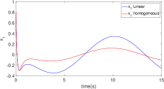
Figure 1: Comparison of $x_{1}$ by linear and homogeneous controller

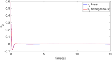
Figure 2: Comparison of $x_{2}$ by linear and homogeneous controller

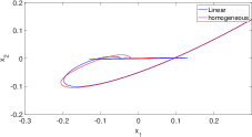
Figure 3: Comparison of trajectory $[x_{1},x_{2}]$ by linear and homogeneous controller

VI-B Experiment results

This experiment is based on the rotary inverted pendulum Quanser Qube Servo-2, where the same model (45) is applied. The system parameters are presented in Table I. Here we consider more physical model of disturbances $D=\begin{bmatrix}0&0&2.53&2.50\end{bmatrix}^{\top}$ and $Q=1$. We use the well tuned linear feedback gain $K=\begin{bmatrix}2&-35&1.5&-3\end{bmatrix}^{\top}$ provided by Quanser to design the homogeneous controller by upgrading the linear one. We obtain

$$X=\left[\begin{smallmatrix}0.00159&0.00002&-0.00275&-0.00018\\ 0.00002&0.00002&0.00011&-0.00004\\ -0.00275&0.00011&0.02492&0.01377\\ -0.00018&-0.00004&0.01377&0.01210\end{smallmatrix}\right]$$ (50)

for $\mu=-0.7$ satisfying (1) (16) and (42) (38).

The experiment is repeated five times to guarantee a fair comparison. The results are presented in the Table II and Table III. It is clear to see that the stabilization precision of $\theta$ and $\alpha$ in $L^{2}$-norm is improved by using the homogeneous controller about $20.22\%$ and $8.3\%$, respectively. The stabilization precision in the $L^{\infty}$-norm is improved about $11.62\%$ and $15.4\%$, respectively. The energy consumption increases about $2.41\%$.

TABLE II: Pendulum stabilization with linear controller

Linear	$\|\theta\|_{L^{\infty}}$	$\|\alpha\|_{L^{\infty}}$	$\|\theta\|_{L^{2}}$	$\|\alpha\|_{L^{2}}$	$\|u\|_{L^{2}}$
Test 1	0.0767	0.0092	0.21333	0.01347	0.79136
Test 2	0.07363	0.00613	0.20377	0.01271	0.7717
Test 3	0.07363	0.00613	0.21414	0.01282	0.67597
Test 4	0.0859	0.0092	0.2379	0.01423	0.74302
Test 5	0.0859	0.0092	0.24353	0.01332	0.60481
Average	0.0792	0.00797	0.2225	0.0133	0.7174

TABLE III: Pendulum stabilization with homogeneous controller

Homogeneous	$\|\theta\|_{L^{\infty}}$	$\|\alpha\|_{L^{\infty}}$	$\|\theta\|_{L^{2}}$	$\|\alpha\|_{L^{2}}$	$\|u\|_{L^{2}}$
Test 1	0.0675	0.00613	0.18762	0.01268	0.6292
Test 2	0.0675	0.00613	0.18695	0.01277	0.77291
Test 3	0.0675	0.00613	0.16906	0.01126	0.71843
Test 4	0.0767	0.0092	0.17481	0.01245	0.76564
Test 5	0.07056	0.00613	0.16912	0.01202	0.78741
Average	0.0700	0.00674	0.1775	0.0122	0.7347

VII Conclusion

This article extends the invariant/attractive ellipsoid method [37, 12, 13] to a class of the generalized homogeneous system. The LMI-based characterization of $\mathbf{d}$-homogeneous invariant/attractive ellipsoid for a linear plant is obtained by the homogeneous control. It shows that, under certain restriction to the structure of perturbations, an optimal (in the sense of the minimal invariant ellipsoid) $\mathbf{d}-$homogeneous invariant/attractive ellipsoid can be upgraded from any conventional invariant/attractive one by properly selecting the dilation $\mathbf{d}$. Despite that theoretically optimal invariant ellipsoids are the same for both linear and homogeneous controllers, the simulation and experiment results show that the optimal homogeneous controller may provide a better precision one under the same conditions/perturbations.

Lemma .1 (Proposition 4.1, [40])

Let $n\geq 3$. Let us consider the homogeneous quadratic forms $f_{i}(x)=x^{\top}A_{i}x$, $i=0,1,2$ with $x\in\mathbb{R}^{n}$ $A_{i}=A_{i}^{\top}\in\mathbb{R}^{n\times n}$, and the numbers $\alpha_{0},\alpha_{1},\alpha_{2}\in\mathbb{R}$, $\alpha_{2}\neq 0$. Let there exist $\mu_{1},\mu_{2}\in\mathbb{R}$ and $x_{0}\in\mathbb{R}^{n}$ such that

$$\mu_{1}A_{1}+\mu_{2}A_{2}\succ 0\text{ and }f_{1}(x_{0})<\alpha_{1},f_{2}(x_{0})=\alpha_{2}.$$

Then the following two claims are equivalent:

• $\exists\tau_{1}\!\geq 0,\exists\tau_{2}\!\in\mathbb{R}$ : $A_{0}\!\preceq\!\tau_{1}A_{1}+\tau_{2}A_{2},\;\;\alpha_{0}\!\geq\!\tau_{1}\alpha_{1}+\tau_{2}\alpha_{2}$;

• $f_{0}(x)\!\leq\!\alpha_{0},\;\;\forall x\in\mathbb{R}^{n}:f_{1}(x)\!\leq\!\alpha_{1},\;f_{2}(x)\!=\!\alpha_{2}$.

References

• [1] V. Utkin, “Variable structure systems with sliding modes,” IEEE Transactions on Automatic control, vol. 22, no. 2, pp. 212–222, 1977.
• [2] V. I. Utkin, Sliding modes in control and optimization.   Springer Science & Business Media, 2013.
• [3] Y. Shtessel, C. Edwards, L. Fridman, A. Levant et al., Sliding mode control and observation.   Springer, 2014, vol. 10.
• [4] V. Utkin, J. Guldner, and J. Shi, Sliding mode control in electro-mechanical systems.   CRC press, 2017.
• [5] G. Zames, “Feedback and optimal sensitivity: Model reference transformations, multiplicative seminorms, and approximate inverses,” IEEE Transactions on automatic control, vol. 26, no. 2, pp. 301–320, 1981.
• [6] Y. V. Orlov and L. T. Aguilar, Advanced $H_{\infty}$ control: Towards nonsmooth theory and applications.   Springer Science & Business Media, 2014.
• [7] H. Kimura, “Robust stabilizability for a class of transfer functions,” IEEE Transactions on Automatic Control, vol. 29, no. 9, pp. 788–793, 1984.
• [8] E. Gershon, U. Shaked, and I. Yaesh, H-infinity control and estimation of state-multiplicative linear systems.   Springer science & business media, 2005, vol. 318.
• [9] D. Bertsekas and I. Rhodes, “Recursive state estimation for a set-membership description of uncertainty,” IEEE Transactions on Automatic Control, vol. 16, no. 2, pp. 117–128, 1971.
• [10] J. Glover and F. Schweppe, “Control of linear dynamic systems with set constrained disturbances,” IEEE Transactions on Automatic Control, vol. 16, no. 5, pp. 411–423, 1971.
• [11] F. Schweppe, “Recursive state estimation: Unknown but bounded errors and system inputs,” IEEE Transactions on Automatic Control, vol. 13, no. 1, pp. 22–28, 1968.
• [12] M. V. Khlebnikov, B. T. Polyak, and V. M. Kuntsevich, “Optimization of linear systems subject to bounded exogenous disturbances: The invariant ellipsoid technique,” Automation and Remote Control, vol. 72, no. 11, pp. 2227–2275, 2011.
• [13] A. Poznyak, A. Polyakov, and V. Azhmyakov, Attractive ellipsoids in robust control.   Springer, 2014.
• [14] S. Boyd, L. El Ghaoui, E. Feron, and V. Balakrishnan, Linear matrix inequalities in system and control theory.   SIAM, 1994.
• [15] A. Polyakov, Generalized Homogeneity in Systems and Control.   Springer, 2020.
• [16] V. Zubov, “On systems of ordinary differential equations with generalized homogenous right-hand sides,” Izvestia vuzov. Mathematica (in Russian), vol. 1, pp. 80–88, 1958.
• [17] M. Kawski, “Homogeneous stabilizing feedback laws,” Control Theory and advanced technology, vol. 6, no. 4, pp. 497–516, 1990.
• [18] H. Hermes, “Nilpotent approximations of control systems and distributions,” SIAM journal on control and optimization, vol. 24, no. 4, pp. 731–736, 1986.
• [19] S. P. Bhat and D. S. Bernstein, “Geometric homogeneity with applications to finite-time stability,” Mathematics of Control, Signals and Systems, vol. 17, pp. 101–127, 2005.
• [20] A. Levant, “Homogeneity approach to high-order sliding mode design,” Automatica, vol. 41, no. 5, pp. 823–830, 2005.
• [21] Y. Orlov, “Finite time stability and robust control synthesis of uncertain switched systems,” SIAM Journal on Control and Optimization, vol. 43, no. 4, pp. 1253–1271, 2004.
• [22] A. Polyakov, D. Efimov, and W. Perruquetti, “Robust stabilization of MIMO systems in finite/fixed time,” International Journal of Robust and Nonlinear Control, vol. 26, no. 1, pp. 69–90, 2016.
• [23] S. Wang, A. Polyakov, and G. Zheng, “Generalized homogenization of linear controllers: Theory and experiment,” International Journal of Robust and Nonlinear Control, vol. 31, no. 9, pp. 3455–3479, 2021.
• [24] ——, “Generalized homogenization of linear observers: Theory and experiment,” International Journal of Robust and Nonlinear Control, vol. 31, no. 16, pp. 7971–7984, 2021.
• [25] M. Kawski, “Families of dilations and asymptotic stability,” in Analysis of Controlled Dynamical Systems: Proceedings of a Conference held in Lyon, France, July 1990.   Springer, 1991, pp. 285–294.
• [26] L. Rosier, “Etude de quelques problèmes de stabilization,” PhD Thesis, Ecole Normale Superieure de Cachan (France), 1993.
• [27] E. Bernuau, “Robustness and stability of nonlinear systems: a homogeneous point of view,” Ph.D. dissertation, Ecole Centrale de Lille, 2013.
• [28] A. Polyakov, “Sliding mode control design using canonical homogeneous norm,” International Journal of Robust and Nonlinear Control, vol. 29, no. 3, pp. 682–701, 2019.
• [29] M. Mera, A. Polyakov, and W. Perruquetti, “Finite-time attractive ellipsoid method: Implicit Lyapunov function approach,” International Journal of Control, vol. 89, no. 6, pp. 1079–1090, 2016.
• [30] K. Zimenko, A. Polyakov, D. Efimov, and W. Perruquetti, “Robust feedback stabilization of linear MIMO systems using generalized homogenization,” IEEE Transactions on Automatic Control, vol. 65, no. 12, pp. 5429–5436, 2020.
• [31] H. Kwakernaak, “$h_{2}$ optimization theory and applications to robust control design,” Annual Reviews in Control, vol. 26, no. 1, pp. 45–56, 2002.
• [32] P. P. Khargonekar, I. R. Petersen, and K. Zhou, “Robust stabilization of uncertain linear systems: quadratic stabilizability and H/sup infinity/control theory,” IEEE Transactions on Automatic control, vol. 35, no. 3, pp. 356–361, 1990.
• [33] A. Polyakov, J.-M. Coron, and L. Rosier, “On homogeneous finite-time control for linear evolution equation in Hilbert space,” IEEE Transactions on Automatic Control, vol. 63, no. 9, pp. 3143–3150, 2018.
• [34] Y. Hong, “H$\infty$ control, stabilization, and input-output stability of nonlinear systems with homogeneous properties,” Automatica, vol. 37, no. 6, pp. 819–829, 2001.
• [35] A. Nekhoroshikh, D. Efimov, A. Polyakov, W. Perruquetti, and I. Furtat, “Finite-time stabilization under state constraints,” in Proc. 60th IEEE Conference on Decision and Control (CDC), 2021.
• [36] E. D. Sontag et al., “Smooth stabilization implies coprime factorization,” IEEE transactions on automatic control, vol. 34, no. 4, pp. 435–443, 1989.
• [37] S. A. Nazin, B. T. Polyak, and M. Topunov, “Rejection of bounded exogenous disturbances by the method of invariant ellipsoids,” Automation and Remote Control, vol. 68, no. 3, pp. 467–486, 2007.
• [38] J. Abedor, K. Nagpal, and K. Poolla, “A linear matrix inequality approach to peak-to-peak gain minimization,” International Journal of Robust and Nonlinear Control, vol. 6, no. 9-10, pp. 899–927, 1996.
• [39] F. Zhang, The Schur complement and its applications.   Springer Science & Business Media, 2006, vol. 4.
• [40] B. T. Polyak, “Convexity of quadratic transformations and its use in control and optimization,” Journal of Optimization Theory and Applications, vol. 99, no. 3, pp. 553–583, 1998.