Beyond Jacobian-based tasks: Extended set-based tasks for multi-task execution and prioritization

Abstract

The ability of executing multiple tasks simultaneously is an important feature of redundant robotic systems. As a matter of fact, complex behaviors can often be obtained as a result of the execution of several tasks. Moreover, in safety-critical applications, tasks designed to ensure the safety of the robot and its surroundings have to be executed along with other nominal tasks. In such cases, it is also important to prioritize the former over the latter. In this paper, we formalize the definition of extended set-based tasks, i.e., tasks which can be executed by rendering subsets of the task space asymptotically stable or forward invariant. We propose a mathematical representation of such tasks that allows for the execution of more complex and time-varying prioritized stacks of tasks using kinematic and dynamic robot models alike. We present and analyze an optimization-based framework which is computationally efficient, accounts for input bounds, and allows for the stable execution of time-varying prioritized stacks of extended set-based tasks. The proposed framework is validated using extensive simulations and experiments with robotic manipulators.

Keywords—Multi-task execution, task prioritization, switching task priorities, optimization-based control

1 Introduction

Safe and effective operation of robotic systems requires the simultaneous execution of multiple tasks. This concurrence, which stems from both application and safety needs, can be achieved thanks to the redundancy of a robotic system, which affords the execution of a task in multiple ways. In the case of a robot manipulator arm, for instance, kinematic redundancy consists in having more degrees of freedom (DOFs) than the ones strictly required to execute the task. This implies the existence of different joint velocities (or configurations) that result in the same end-effector velocity (or configuration). For a multi-robot system, the robotic units of which it is comprised and their interchangeability translate into an inherent redundancy of the system. For an extended discussion on redundancy see, for example, [MR13, SHV⁺06, SSVO10].

During the operation of the robotic system, some tasks may take precedence over others. Typically, preserving the safety of the system and its surroundings is more critical than satisfying application-specific objectives. This hierarchy is established in the so-called task stack, used by the robot controller to ensure the prioritized execution of tasks. This way, while high-priority tasks are being executed, the redundancy of the system is exploited to achieve, if possible, lower-priority ones. Moreover, the task hierarchy need not be static. For instance, this can be needed to accommodate the evolution of the objectives dictated by the environment/application, or due to exogenous factors (such as the supervisory control of a human operator). In any case, the robot controller must be able to react to these changes.

The execution of prioritized stacks of tasks by exploiting the redundancy of the system has been proposed in [SS91] and extensively studied since then (see, e.g., [BB98, BB04, EMW14], just to name a few). In these works, a task is associated to a Jacobian matrix, which relates the velocities of the robot joints to the velocities of the point required to execute the task. While the resulting formulation is rigorous, starting from the definition of a Jacobian matrix in order to specify a task is not always intuitive.

In this paper, we propose an optimization-based approach to the analysis and synthesis of the (possibly time-varying) prioritized execution of extended set-based (ESB) tasks—a more expressive description of the tasks introduced in [NMS⁺20], which leverages set stability and safety as building blocks to define robotic tasks. Moreover, the proposed approach is applied to both kinematic and dynamic robot models, allowing torque control of robotic manipulators, and accounting for input constraints, such as torque saturation.

The paper is organized as follows. The remainder of this section is devoted to the comparison of the approach proposed in this paper with existing methods and algorithms for the prioritized execution of multiple robotic tasks. Section 2 presents the concept of ESB tasks, including the required mathematical background, and analyzes the inter-task relationships, generalizing the concepts of dependent, independent, and orthogonal tasks. In Section 3, we describe the approach proposed in this paper for the prioritized execution of multiple tasks. Section 4 deals with time-varying task priorities, while Section 5 shows how the proposed approach can be employed for dynamic robot models which include joint torque saturation. In Section 6, the results of extensive simulations and experiments with real robotic platforms are reported. Section 7 concludes the paper.

1.1 Related Work

1.1.1 Redundancy

Robotic systems that possess more DOFs than the ones strictly required to execute a given task are defined as redundant. In this sense, redundancy is not an inherent property of the robotic system itself rather it is related to the dimension of the task space (e.g., equal to 2 for a planar positioning task) being lower than the dimension of the configuration space of the robot (e.g. equal to the number of joints of a manipulator arm). For instance, for robot manipulators a task typically consists in following an end-effector motion trajectory requiring 6 DOFs, thus a 7-joint robotic arm is usually used as an example of an inherently redundant manipulator. Thus, when this condition is met, the additional DOFs can be conveniently exploited for the optimization of some performance objective, or for the simultaneous execution of other tasks besides the main one ([SSVO10]). In this respect, the redundant DOFs can be exploited to allow a more flexible and adaptive execution of tasks in constrained environments that require avoiding obstacles, for instance. Robotic systems like humanoids, quadruped robots, or mobile manipulators are examples of robotic systems equipped with a large number of DOFs to fulfill these needs.

Typically, one might want to assign different priorities to tasks or objectives, thus requiring control algorithms capable of achieving them while respecting a hierarchical structure ([NHY87]). The following sections illustrate the prior work in this field.

1.1.2 Task Priorities Using Jacobian-based Approaches

Methods for redundancy resolution with prioritized tasks have been thoroughly developed in the last decades. At the differential kinematic level, as an infinite number of joint velocities exist that realize a given task velocity, a criterion must be utilized to select one of them. The use of the (right) pseudoinverse of the Jacobian matrix guarantees the exact reconstruction of the task velocity with the minimum-norm joint velocities. Most methods calculate joint velocities as the general solution of an undetermined linear system, i.e., using the generalized inverse of the task Jacobian plus a velocity vector lying in its null-space. Building upon this concept, a general framework for managing multiple tasks in highly redundant robotic systems, exploiting their kinematic redundancies is presented in [SS91].

By exploiting the nullspace of the Jacobian matrix, one can find additional velocity control inputs to execute secondary tasks without interfering with the primary/critical/main objectives. Several works have focused on determining these additional inputs, starting for example from the gradient of a scalar function (representing the secondary objective) and projecting it onto the null-space of the Jacobian not to affect the primary task ([MCR96]). In this way, tasks are effectively prioritized: the primary task is always fulfilled, while the secondary is accomplished to the extent allowed by the execution of the primary task. This idea was used in [Chi97] to keep the joint angles within their physical limits, avoiding obstacles and singular configurations.

As mentioned in the previous section, this approach is rigorous and it has been successfully employed for different robotic systems, including robotic arms, legged robots, and multi-robot systems. More recently, however, different paradigms have been proposed in order to achieve the concurrent execution of multiple tasks, including the null-space-based behavioral control ([AAC09]) and the set-based tasks, i.e., tasks with a range of valid values ([MAT⁺16]), where the authors give the conditions under which the concurrent execution of multiple tasks is guaranteed.

1.1.3 Transitions Between Different Prioritized Stacks of Tasks

Approaches to enforce a hierarchy among the executed tasks can be then categorized into strict and soft. Strict hierarchies guarantee that the execution of a task at lower priority does not influence the execution of a task at higher priority. This, however, can easily lead to discontinuities of the robot controller during the switch between stacks of tasks ([AAC09, KWMK11, SC16]). The soft task hierarchy enforcement, instead, can guarantee continuous transitions between stacks of tasks, at the expense of letting tasks at lower priorities influence tasks at higher priorities ([SCRC19]).

In this paper, we opt for a soft task hierarchy, since we aim at designing a controller that allows for smooth, stable, and efficient transitions between stacks of tasks. Moreover, we give the conditions under which the influence of low-priority tasks on the execution of tasks at higher priority is not existent.

1.1.4 Optimization-based Approaches

Set-based tasks were introduced in [MAT⁺16] in order to consider unilateral constraints. This has been shown to be useful for robot manipulators in order to encode both operational and joint space tasks and constraints ([DLAAC18]). Inequality constraints are usually difficult to be directly dealt with in analytical approaches. Therefore, solutions that resort to numerical optimization methods which are more or less efficiently solvable in online settings have been proposed in [MRC09, LTP16, BP20], and in [MTAP15], where the authors also prove the stability of the simultaneous execution of several tasks.

The work proposed in this paper also leverages optimization techniques to synthesize the robot controller. In particular, the execution of multiple prioritized tasks is formulated as a single convex quadratic program.

1.2 Contributions

The main contributions of this paper are summarized as follows.

1. We show that ESB tasks are an extension of Jacobian-based tasks, by deriving the conditions for dependent, independent, and orthogonal ESB tasks.

2. The stability analysis of the prioritized execution of stack of ESB tasks is carried out and shown to be independent of the choice of specific gains.

3. The proposed method extends to the dynamic model of robotic systems which include input torque bounds.

4. We propose a systematic way of encoding prioritized stacks of tasks using prioritization matrices.

5. Finally, we carry out the stability analysis in the case of switching between two distinct stacks of tasks.

2 Extended Set-based Task Execution

In this section, standard Jacobian-based tasks are briefly introduced. The concept of ESB tasks is then discussed and an optimization-based framework to execute multiple such tasks simultaneously is presented. Moreover, the characterizing conditions for the various types of inter-task relationships (orthogonality, independence, and dependence) are derived for this new class of tasks.

Consider a $N$-DOF manipulator and let $q\in\mathcal{Q}$ denote the joint configuration, an element of the $N$-dimensional configuration space $\mathcal{Q}$, and $\dot{q}\in\mathbb{R}^{N}$, the joint velocity vector. Let $m$ denote the dimension of the task space $\mathcal{T}$. We start by considering robots that can be modeled as kinematic systems, i.e., that are endowed with a low-level high-gain controller that takes care of reproducing the desired velocity inputs. Let $\sigma\in\mathcal{T}$ denote the task variable to be controlled, defined as:

$$\sigma=k(q),$$ (1)

where the smooth map $k:\mathcal{Q}\rightarrow\mathcal{T}$ represents the task forward kinematics. It follows that

$$\dot{\sigma}=J(q)\dot{q},$$ (2)

where $J\colon\mathcal{Q}\to\mathbb{R}^{m\times N}$ is the task Jacobian defined as $J(q)=\frac{\partial k}{\partial q}(q)$. The tasks consisting in executing the joint velocities $\dot{q}$ satisfying the relation in (2) to make $\sigma(t)$ equal to a desired task variable trajectory $\sigma_{d}(t)$ will be referred to as Jacobian-based tasks. A Jacobian-based task is accomplished when the task variable $\sigma(t)$ tracks the desired $\sigma_{d}(t)$.

As discussed in Section 1, there is often a need to concurrently execute multiple Jacobian-based tasks. Towards this end, let $\sigma_{i}=k_{i}(q)\in\mathbb{R}^{m_{i}}$—the task space is an $m_{i}$-dimensional Euclidean space—be the task variables associated to $M$ tasks, where $i=\{1,\dots,M\}$. In the following, we will use $m$ to denote the sum of dimensions of task variables, $m=\sum_{i=1}^{M}m_{i}$. The evolution of each task variable can then be represented as

$$\dot{\sigma}_{i}=J_{i}(q)\dot{q},\quad J_{i}(q)=\frac{\partial k_{i}}{\partial q}(q),$$ (3)

where $J_{i}(q)$ is the $i$-th task Jacobian.

For more details on Jacobian-based tasks, we address the interested reader to, e.g., [Ant09] and references therein. Next, we introduce the concept of ESB tasks.

2.1 Extended Set-based Tasks

When considering Jacobian-based tasks, the main approach for executing a task is to drive the task variable towards a desired value (see [Ant09]). Nevertheless, this approach defines tasks based on the velocities of the task variable, $\dot{\sigma}$. It is often more convenient to define tasks that can be accomplished by making the task variable approach a desired set of the task space (stability) or constraining the task variable to remain within a given set (safety). While the Jacobian-based tasks do not lend themselves to this type of task definition, the ESB tasks used in this paper do.

Set-based tasks have been introduced in [EMW14] for representing tasks that can be executed by letting the task variables remain in a desired area of satisfaction. Some examples of set-based tasks are joint limits or singularity avoidance, where the area of satisfaction is not a specific configuration but rather the set of joint values that are not including joint-limit values or singularity configurations, respectively.

There is an analogy between the set-based interpretation of tasks and the concept of forward invariance in the dynamical systems literature ([Kha15]). In fact, executing a set-based task is equivalent to enforcing the state of the robot to remain in a desired set, i.e., making the set forward invariant. Exploiting this analogy, it is possible to extend the definition of set-based tasks in order to include the possibility of executing a task evolving towards a set, which corresponds to the concept of set-stability.

Definition 1 ((ESB Task)).

An ESB task is a task characterized by a set $\mathcal{C}\subset\mathcal{T}$, where $\mathcal{T}$ is the task space, which can be expressed as the zero superlevel set of a continuously differentiable function $h\colon\mathcal{T}\times\mathbb{R}_{\geq 0}\to\mathbb{R}$ as follows:

$$\mathcal{C}=\{\sigma\in\mathcal{T}\colon h(\sigma,t)\geq 0\}.$$ (4)

The goal is rendering the time-varying set forward invariant and asymptotically stable.

The definition of ESB task generalizes the one of Jacobian-based task as shown in the following example:

Example 1 ((Generalization of Jacobian-based tasks—Part I)).

Consider the Jacobian-based task encoded by the following differential kinematic equation:

$$\dot{\sigma}_{d}(t)=J_{d}(q)\dot{q}(t),$$ (5)

where $\dot{\sigma}_{d}(t)$ is the value at time $t$ of a desired task variable we want the robot to track. Let the function $h$ used in Definition 1 be defined as

$$h(\sigma,t)=-\frac{1}{2}\|\sigma-\sigma_{d}(t)\|^{2},$$ (6)

where the function $\sigma_{d}(t)$ is given by $\sigma_{d}(t)=\int_{0}^{t}\dot{\sigma}_{d}(\tau)\mathrm{d}\tau$. Assuming that the $\dot{\sigma}_{d}$ specified in (5) is a continuous function of time, $h$ is continuously differentiable with respect to both its arguments, as specified in Definition 1.

We notice that the set $\mathcal{C}$, zero superlevel of $h$, at time $t$ is given by $\{\sigma\in\mathcal{T}\colon\sigma=\sigma_{d}(t)\}$. Therefore, rendering $\mathcal{C}$ asymptotically stable and forward invariant corresponds to the original Jacobian-based task being executed.

Given a task $\sigma=k(q)$, the following control affine system can be employed to define the evolution of the robot as well as the task:

$$\begin{cases}\dot{x}=f(x)+g(x)u\\ \sigma=k(x),\end{cases}$$ (7)

where, as before, the smooth map $k:\mathcal{Q}\rightarrow\mathcal{T}$ represents the task forward kinematics. This control affine form encompasses the kinematic robot model (2) by setting $x=q$, $f=0$, $g=J$ and $u=\dot{q}$. As will be shown in Section 5, the standard dynamic model of a robot manipulator is also affine in the control input (joint torques), and can be therefore represented by (7).

Starting from the methodology for task execution proposed in [NE19], we now develop a strategy for the execution of ESB tasks. According to Definition 1, in order to accomplish an ESB task, it is necessary to control the robot for making the satisfaction set $\mathcal{C}$ attractive and forward invariant. As shown in [NE19, NMHE19], this behavior can be formulated as a constrained optimization problem where the control input is chosen to enforce the task satisfaction. This desired behavior can be formalized using Control Barrier Functions (CBFs) that render the desired set forward invariant and stable (see [ACE⁺19]). These properties are briefly recalled in the following.

Definition 2 ((Output Time-Varying CBF, based on [ACE⁺19] and [NE21])).

Let $\mathcal{C}\subset\mathcal{D}\subset\mathcal{T}$ be the superlevel set of a continuously differentiable function $h:\mathcal{D}\times\mathbb{R}_{\geq 0}\to\mathbb{R}$, contained in a domain $\mathcal{D}$. Then, $h$ is an output time-varying CBF—in the following referred to simply as CBF—if there exists a Lipschitz continuous extended class $\mathcal{K}_{\infty}$ function $\gamma$ ([ACE⁺19]) such that for the control system (7), for all $\sigma\in\mathcal{D}$,

$$\sup_{u\in\mathcal{U}}\left\{\frac{\partial h}{\partial t}+\frac{\partial h}{\partial\sigma}\frac{\partial\sigma}{\partial x}f(x)+\frac{\partial h}{\partial\sigma}\frac{\partial\sigma}{\partial x}g(x)u\right\}\geq-\gamma(h(\sigma,t)).\hskip 7.11317pt$$ (8)

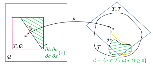
Figure 1: Pictorial representation of the differential constraints introduced in (8) for the time-invariant case. The set $\mathcal{C}$ to be rendered forward invariant and asymptotically stable is a subset of the task space $\mathcal{T}$. The constraint (8) can be equivalently written as $\frac{\partial h}{\partial\sigma}\dot{\sigma}\geq-\gamma(h(\sigma,t))$, which is a affine in $\dot{\sigma}$, constraining it to lie in a half plane in the tangent space of the task space, $T_{\sigma}\mathcal{T}$. The velocity $\dot{\sigma}$ is transformed into the velocity $\dot{x}$ in the tangent space $T_{x}\mathcal{Q}$ of the state space. In this space, the constraint (8) is affine in $\dot{x}$, which has to lie in the green hatched half plane.

The constraint (8) is pictorially represented in Fig 1. Exploiting this definition of CBFs, it is possible to state the following result.

Theorem 1 ((Based on [ACE⁺19] and [NE21])).

Let $\mathcal{C}\subset\mathcal{T}$ be a set defined as the superlevel set of a continuously differentiable function $h:\mathcal{D}\times\mathbb{R}_{\geq 0}\to\mathbb{R}$. If $h$ is a CBF on $\mathcal{D}$ according to Definition 2, then any Lipschitz continuous controller $u(x,t)\in\mathcal{V}(x,t)$, where $\mathcal{V}(x,t)=\{u(x,t)\colon\frac{\partial h}{\partial t}+\frac{\partial h}{\partial\sigma}\frac{\partial\sigma}{\partial x}f(x)+\frac{\partial h}{\partial\sigma}\frac{\partial\sigma}{\partial x}g(x)u+\gamma(h(\sigma,t))\geq 0\}$, for the system (7) renders the set $\mathcal{C}$ forward invariant. Additionally, the set $\mathcal{C}$ is asymptotically stable in $\mathcal{D}$.

Definition 2 and Theorem 1 show how CBFs can ensure the forward invariance and the asymptotic stability of a desired subset of the task space $\mathcal{T}$. One possible control input for executing a desired task can be found by solving the following convex Quadratic Program (QP):

$$\operatorname*{minimize~{}}_{u} \|u\|^{2}$$ (9)

$$\operatorname*{subject\,to~{}} \frac{\partial h}{\partial t}+\frac{\partial h}{\partial\sigma}\frac{\partial\sigma}{\partial x}f(x)+\frac{\partial h}{\partial\sigma}\frac{\partial\sigma}{\partial x}g(x)u$$

$$+\gamma(h(\sigma,t))\geq 0,$$

where $h(\sigma,t)$ is the CBF representing the set $\mathcal{C}$ as shown in Definition 1.

Example 2 ((Generalization of Jacobian-based tasks—Part II)).

The task introduced in Example 1 can be executed by ensuring the asymptotic stability of the set $\mathcal{C}$ defined in (4) using the CBF in (6). This property corresponds to the following condition: $\sigma(t)\to\sigma_{d}(t)$ as $t\to\infty$.

We can use the optimization-based formulation (9) in order to synthesize a velocity controller $\dot{q}$ that renders the set $\mathcal{C}$ asymptotically stable as well as forward invariant. The controller, solution of the following optimization program

$$\operatorname*{minimize~{}}_{\dot{q}} \|\dot{q}\|^{2}$$ (10)

$$\operatorname*{subject\,to~{}} (\sigma-\sigma_{d}(t))^{\sf T}J_{0}(q)\dot{q}\geq$$

$$-\gamma(h(\sigma,t))-(\sigma-\sigma_{d}(t))^{\sf T}\dot{\sigma}_{d}(t),$$

guarantees the asymptotic stability of $\mathcal{C}$, which is equivalent to the execution of the Jacobian-based task (5). Notice how, owing to the convexity of (10), a controller can be synthesized very efficiently, with bounds on the computational time and on the error of the numerical solution ([BV04]). For these reasons, executing a task by implementing the controller solution of the convex optimization program (10) is amenable in applications where real-time constraints are prescribed, such as in the control of robotic manipulators or in safety-critical scenarios.

The formulation in (9) can be extended to model the execution of multiple tasks concurrently. Each task is specified as a constraint in the optimization problem. Formally, let $T_{1},\dots,T_{M}$ be the tasks to be executed, with $\sigma_{i}$ denoting the task variable corresponding to task $T_{i}$. The execution of task $T_{i}$ is encoded by the CBF $h_{i},~{}i\in\{1,\dots,M\}$. The execution of the set of $M$ tasks can be realized through the solution to the following optimization problem:

$$\operatorname*{minimize~{}}_{u,\delta} \|u\|^{2}+l\|\delta\|^{2}$$ (11)

$$\operatorname*{subject\,to~{}} \frac{\partial h_{i}}{\partial t}+\frac{\partial h_{i}}{\partial\sigma_{i}}\frac{\partial\sigma_{i}}{\partial x}f(x)+\frac{\partial h_{i}}{\partial\sigma_{i}}\frac{\partial\sigma_{i}}{\partial x}g(x)u$$

$$+\gamma_{i}(h_{i}(\sigma_{i},t))\geq-\delta_{i}\quad\forall i\in\{1,\ldots,M\}.$$

Notice how each task is associated with a slack variable $\delta_{i}$, with $\delta=[\delta_{1},\ldots,\delta_{M}]^{\sf T}$. This allows us, first of all, to ensure the feasibility of the optimization program (11). In fact, consider the case when the $M$ tasks cannot be executed concurrently, i.e., the half-spaces defined by the affine inequality constraints in (11) without $\delta_{i}$ do not intersect. If slack variables are removed from the constraints, then the optimization program may become infeasible. By employing slack variables to relax task constraints and adding the term $l\|\delta\|^{2}$ in the cost of (11), the control input solution of the optimization program results in the execution of multiple tasks to the best of the capabilities of a robotic system (see [NMHE19]).

In the following section, we analyze the relationship between tasks that characterizes the feasibility of their concurrent execution without the need of slack variables. Moreover, as will be shown in Section 3, slack variables will be leveraged to enforce relative priorities between tasks.

2.2 Analyzing Inter-Task Relationships

In order to evaluate if a set of tasks can be executed concurrently, it is necessary to characterize the interdependence properties of the tasks, intended as in Definition 1, i.e., ESB tasks. In this section, the concepts of orthogonality, independence, and dependence—commonly used in the the literature for describing the relationships between Jacobian-based tasks—are extended to ESB tasks. In the following, we first recall these concepts for Jacobian-based tasks.

Consider two Jacobian-based tasks encoded by $\sigma_{i}(q)\in\mathbb{R}^{m_{i}}$, $\sigma_{j}(q)\in\mathbb{R}^{m_{j}}$, whose velocities are expressed by the mappings $\dot{\sigma}_{i}(q)=J_{i}(q)\dot{q}$, $\dot{\sigma}_{j}(q)=J_{j}(q)\dot{q}$, with $J_{i}\neq 0$ and $J_{j}\neq 0$. The following definitions are used to recall the three distinct types of inter-task relationships discussed in the literature.

Definition 3 ((Jacobian-based task orthogonality, based on [Ant09])).

Two Jacobian-based tasks $\sigma_{i}(q)$ and $\sigma_{j}(q)$ are orthogonal (or annihilating) if

$$J_{i}(q)J_{j}(q)^{\sf T}=0_{m_{i}\times m_{j}},\quad\forall q\in\mathcal{Q},$$ (12)

where $0_{m_{i}\times m_{j}}$ is the $m_{i}\times m_{j}$ null matrix.

Definition 4 ((Jacobian-based task independence, based on [Ant09])).

Two Jacobian-based tasks $\sigma_{i}(q)$ and $\sigma_{j}(q)$ are independent if

$$~{}\mathrm{rank}(J_{i}^{\sf T}(q))+\mathrm{rank}(J_{j}^{\sf T}(q))$$ (13)

$$= ~{}\mathrm{rank}\left(\begin{bmatrix}J_{i}^{\sf T}(q)&J_{j}^{\sf T}(q)\end{bmatrix}\right),\quad\forall q\in\mathcal{Q}.$$

Definition 5 ((Jacobian-based task dependence, based on [Ant09])).

Two Jacobian-based tasks $\sigma_{i}(q)$ and $\sigma_{j}(q)$ are dependent if

$$\exists\,q\in\mathcal{Q}~{}\colon ~{}\mathrm{rank}(J_{i}(q)^{\sf T})+\mathrm{rank}(J_{j}(q)^{\sf T})$$ (14)

$$> ~{}\mathrm{rank}\left(\begin{bmatrix}J_{i}(q)^{\sf T}&J_{j}(q)^{\sf T}\end{bmatrix}\right).$$

Remark 1.

Orthogonal Jacobian-based tasks are independent.

Remark 2.

It is worth noting that the three conditions of orthogonality, dependence, and independence may be given by resorting to the pseudoinverse of the corresponding Jacobians instead of the transpose. In fact, they share the same span.

We now derive the conditions required to characterize the inter-task relationships of orthogonality, dependence, and independence for ESB tasks. In particular, consider two ESB tasks encoded by the CBFs $h_{i}$ and $h_{j}$, with $\frac{\partial h_{i}}{\partial q}\neq 0$ and $\frac{\partial h_{j}}{\partial q}\neq 0$.

Definition 6 ((ESB task orthogonality)).

Two ESB tasks encoded by the CBFs $h_{i}$ and $h_{j}$ are orthogonal if

$$\frac{\partial h_{i}}{\partial q}\frac{\partial h_{j}}{\partial q}^{\sf T}=0,\quad\forall q\in\mathcal{Q}.$$ (15)

Definition 6 is well posed since it generalizes the concept of orthogonality in Definition 3. This is shown by the following result:

Proposition 1 ((Generalization of task orthogonality)).

If two Jacobian-based tasks $\dot{\sigma}_{i}=J_{i}(q)\dot{q}$ and $\dot{\sigma}_{j}=J_{j}(q)\dot{q}$ are orthogonal according to Definition 3, the corresponding ESB tasks $h_{i}$ and $h_{j}$ constructed as in Example 1 are orthogonal according to Definition 6. The converse is not necessarily true.

Proof.

To prove that

$$J_{i}(q)J_{j}(q)^{\sf T}=0\implies\frac{\partial h_{i}}{\partial q}\frac{\partial h_{j}}{\partial q}^{\sf T}=0,$$ (16)

it is sufficient to expand (15) as follows:

$$\frac{\partial h_{i}}{\partial q}\frac{\partial h_{j}}{\partial q}^{\sf T}=\frac{\partial h_{i}}{\partial\sigma_{i}}J_{i}(q)J_{j}(q)^{\sf T}\frac{\partial h_{j}}{\partial\sigma_{j}}^{\sf T}=0.$$ (17)

One can see how, whenever $J_{i}(q)$ or $J_{j}(q)$ have a non-trivial nullspace, the converse need not be true. ∎∎

Proposition 1 shows how ESB tasks can generalize Jacobian-based tasks. This will be confirmed by the following results on dependence and independence.

Definition 7 ((ESB task independence)).

Two ESB tasks encoded by the CBFs $h_{i}$ and $h_{j}$ are independent if

$$\mathrm{rank}\left(\begin{bmatrix}\dfrac{\partial h_{i}}{\partial q}^{\sf T}&\dfrac{\partial h_{j}}{\partial q}^{\sf T}\end{bmatrix}\right)=2,\quad\forall q\in\mathcal{Q}.$$ (18)

Remark 3.

Orthogonal ESB tasks are independent.

Definition 7 is well posed since it generalizes Definition 4 as shown by next proposition.

Proposition 2 ((Generalization of task independence)).

If two Jacobian-based tasks $\dot{\sigma}_{i}=J_{i}(q)\dot{q}$ and $\dot{\sigma}_{j}=J_{j}(q)\dot{q}$ are independent according to Definition 4, the corresponding ESB tasks $h_{i}(\sigma_{i}(q))$ and $h_{j}(\sigma_{j}(q))$ are independent according to Definition 7). The converse is not necessarily true.

Proof.

To prove that

$$~{}\mathrm{rank}(J_{i}(q)^{\sf T})+\mathrm{rank}(J_{j}(q)^{\sf T})$$ (19)

$$= ~{}\mathrm{rank}\left(\begin{bmatrix}J_{i}(q)^{\sf T}J_{j}(q)^{\sf T}\end{bmatrix}\right)$$

$$\implies \mathrm{rank}\left(\begin{bmatrix}\dfrac{\partial h_{i}}{\partial q}^{\sf T}&\dfrac{\partial h_{j}}{\partial q}^{\sf T}\end{bmatrix}\right)=2,$$

recall that subspace independence means

$$\mathrm{span}(J_{i}(q)^{\sf T})\cap\mathrm{span}(J_{j}(q)^{\sf T})=\{0\}.$$ (20)

Since

$$\frac{\partial h_{i}}{\partial q}^{\sf T}=J_{i}^{\sf T}\frac{\partial h_{i}}{\partial\sigma_{i}}^{\sf T}\in\mathrm{span}(J_{i}(q)^{\sf T})$$ (21)

and

$$\frac{\partial h_{j}}{\partial q}^{\sf T}=J_{j}^{\sf T}\frac{\partial h_{j}}{\partial\sigma_{j}}^{\sf T}\in\mathrm{span}(J_{j}(q)^{\sf T})$$ (22)

we can claim independence of the vectors $\displaystyle\frac{\partial h_{i}}{\partial q}^{\sf T}$ and $\displaystyle\frac{\partial h_{j}}{\partial q}^{\sf T}$. The converse is not necessarily true whenever $J_{i}(q)$ or $J_{j}(q)$ have a non-trivial nullspace. ∎∎

Finally, the task dependence concept can be also generalized to ESB tasks.

Definition 8 ((ESB task dependence)).

Two ESB tasks encoded by the CBFs $h_{i}$ and $h_{j}$ are dependent if

$$\exists\,q\in\mathcal{Q}~{}\colon~{}\mathrm{rank}\left(\begin{bmatrix}\dfrac{\partial h_{i}}{\partial q}^{\sf T}&\dfrac{\partial h_{j}}{\partial q}^{\sf T}\end{bmatrix}\right)=1.$$ (23)

Remark 4.

The task orthogonality condition (15) corresponds to the geometric condition

$$\angle\left(\frac{\partial h_{i}}{\partial q}^{\sf T},\frac{\partial h_{j}}{\partial q}^{\sf T}\right)=\frac{\pi}{2}.$$ (24)

The task independence condition (18) corresponds to the geometric condition

$$\angle\left(\frac{\partial h_{i}}{\partial q}^{\sf T},\frac{\partial h_{j}}{\partial q}^{\sf T}\right)\in\left(0,\pi\right],$$ (25)

while dependence corresponds to

$$\angle\left(\frac{\partial h_{i}}{\partial q}^{\sf T},\frac{\partial h_{j}}{\partial q}^{\sf T}\right)=0.$$ (26)

The above presented results for ESB tasks and their connections with Jacobian-based tasks are summarized in Table 1.

Table 1: Inter-task Relationships: orthogonality, independence, and dependence for Jacobian-based and ESB tasks

Relationship	Jacobian-based tasks	ESB tasks
Orthogonality	$J_{i}J_{j}^{\sf T}=0_{m_{i}\times m_{j}}$	$\dfrac{\partial h_{i}}{\partial q}\dfrac{\partial h_{j}}{\partial q}^{\sf T}=0$
Independence	$\mathrm{rank}(J_{i}^{\sf T})+\mathrm{rank}(J_{j}^{\sf T})=\mathrm{rank}\left(\begin{bmatrix}J_{i}^{\sf T}&J_{j}^{\sf T}\end{bmatrix}\right)$	$\mathrm{rank}\left(\begin{bmatrix}\dfrac{\partial h_{i}}{\partial q}^{\sf T}&\dfrac{\partial h_{j}}{\partial q}^{\sf T}\end{bmatrix}\right)=2$
Dependence	$\exists\,q\in\mathcal{Q}~{}\colon~{}\mathrm{rank}(J_{i}^{\sf T})+\mathrm{rank}(J_{j}^{\sf T})>\mathrm{rank}\left(\begin{bmatrix}J_{i}^{\sf T}J_{j}^{\sf T}\end{bmatrix}\right)$	$\exists\,q\in\mathcal{Q}~{}\colon~{}\mathrm{rank}\left(\begin{bmatrix}\dfrac{\partial h_{i}}{\partial q}^{\sf T}\dfrac{\partial h_{j}}{\partial q}^{\sf T}\end{bmatrix}\right)=1$

3 Prioritized Multi-Task Execution

As discussed earlier, to effectively handle the simultaneous execution of tasks which cannot be executed concurrently, we introduced slack variables in the optimization program (11) used to synthesize the robot controller. As shown in this section, the introduction of slack variables can be used to enforce prioritization among tasks. This section extends the multi-task execution framework presented in the previous section to introduce prioritized execution and proves the stability properties of such a framework.

3.1 Prioritized Execution of Extended Set-based Task Stacks

Within the multi-task execution framework introduced in (11), a natural way to introduce priorities is to enforce relative constraints among the slack variables corresponding to the different tasks that need to be performed. For example, if the robot were to perform task $T_{i}$ with the highest priority (often referred to using the partial order notation $T_{i}\prec T_{j}$ $\forall j\in\{1,\ldots,M\},j\neq i$) the additional constraint $\delta_{i}\leq\delta_{j}/\kappa$, $\kappa>1$, $\forall j\in\{1,\ldots,M\},j\neq i$ in (11) would imply that task $T_{i}$ is relaxed to a lesser extent—thus performed with a higher priority—than the other tasks. The relative scale between the functions $h_{i}$ encoding the tasks should be considered while choosing the value of $\kappa$.

Formally, prioritizations among tasks can be encoded through an additional linear constraint $K\delta\leq 0$ to be enforced in the optimization problem (11). In the following, we refer to ${K\in\mathbb{R}^{(M-1)\times M}}$ as the prioritization matrix, which encodes the pairwise inequality constraints among the slack variables, thus fully specifying the prioritization stack among the tasks. Example 3 illustrates the use of the prioritization matrix $K$ to define a stack of tasks, in which tasks are ordered according to their priority.

Example 3 ((Prioritization matrix)).

The tasks are encoded by the CBFs

$$h_{i}:\mathcal{T}_{i}\times\mathbb{R}_{\geq 0}\to\mathbb{R},\quad\quad i\in\{1,2,3\},$$ (27)

where $\mathcal{T}_{i}$ is the task space related to task $i$. The values of the entries of the prioritization matrix $K$ have to be chosen in order to encode the desired priorities between the tasks. For instance, if the stack of tasks is $T_{1}\prec T_{3}\prec T_{2}$—i.e., task $T_{1}$ has to be executed with priority greater than task $T_{3}$, which, in turn, has to be executed with priority greater than $T_{2}$—then the rows of $K$ have to encode the constraints $\delta_{1}\leq\delta_{3}/\kappa$ and $\delta_{3}\leq\delta_{2}/\kappa$, i.e.,

$$K=\begin{bmatrix}1&0&-1/\kappa\\ 0&-1/\kappa&1\end{bmatrix}.$$ (28)

For $M$ extended-set based tasks with task variables $\sigma_{i}$ and whose execution is characterized by the CBFs $h_{i}$, $i\in\{1,\ldots,M\}$, the execution of the prioritized task stack can then be encoded via the following optimization problem which features the prioritization matrix $K$ defined as above:

$$\operatorname*{minimize~{}}_{u,\delta} \|u\|^{2}+l\|\delta\|^{2}$$ (29)

$$\operatorname*{subject\,to~{}} \frac{\partial h_{i}}{\partial t}+\frac{\partial h_{i}}{\partial\sigma_{i}}\frac{\partial\sigma_{i}}{\partial x}f(x)+\frac{\partial h_{i}}{\partial\sigma_{i}}\frac{\partial\sigma_{i}}{\partial x}g(x)u$$

$$+\gamma_{i}(h_{i}(\sigma_{i},t))\geq-\delta_{i},\quad\forall i\in\{1,\ldots,M\}$$

$$K\delta\leq 0.$$

Example 3 shows how one can construct a prioritization matrix associated with an ordered stack of tasks. As long as the prioritization matrix is constructed following this procedure, then there are no issues concerning the feasibility of the QP (29). That is because the prioritization matrix only enforces relative constraints between components of the prioritization vector $\delta$; therefore, it is straightforward to see that there always exist large enough components of $\delta$ so that all constraints in (29) are satisfied.

Nevertheless, since these constraints represent tasks to be executed by a robot, we are concerned with the quality of execution of these tasks. A large value of $\delta_{i}$, as a matter of fact, might result in task $i$ not being executed. Therefore, we would like the values of $\delta_{i}$ to be as small as possible, possibly zero, at least when task $i$ has highest priority. Because of the prioritization constraint $K\delta\leq 0$, however, the component of $\delta$ corresponding to the task at highest priority is constrained by the component of $\delta$ corresponding to the tasks at lower priorities. By increasing the constant $l$ in (29) the desired behavior—tasks at the highest priority being perfectly executed, with a negligible component of $\delta$ compared to the value of the CBF encoding the task—can be achieved.

Remark 5 ((Feasibility of the prioritization stack)).

Although (29) is always feasible, the execution of the optimal control input $u^{*}$, might not lead to a convergent behavior since the ratio between the components of $\delta$, prescribed by the constraint $K\delta\leq 0$, might be unrealizable when $\dot{h}(x,u^{*})=0$. In the following section we present an alternative mechanism to solve this problem based on the relaxation of the prioritization constraint.

3.2 Automatic Prioritization Stack

Assume that $M$ tasks are ordered by priority, so that task $T_{i}$ has higher priority than task $T_{i+1}$, and consider the following optimization program:

$$\operatorname*{minimize~{}}_{u,\delta,v} \|u\|^{2}+l_{\delta}\|\delta\|^{2}+l_{v}\|v\|^{2}$$ (30)

$$\operatorname*{subject\,to~{}} \frac{\partial h_{i}}{\partial t}+\frac{\partial h_{i}}{\partial\sigma_{i}}\frac{\partial\sigma_{i}}{\partial x}f(x)+\frac{\partial h_{i}}{\partial\sigma_{i}}\frac{\partial\sigma_{i}}{\partial x}g(x)u$$

$$+\gamma_{i}(h_{i}(\sigma_{i},t))\geq-\delta_{i},\quad\forall i\in\{1,\ldots,M\}$$

$$K\delta\leq Vv.$$

The optimization program in (30) is similar to the one in (29) except for the relaxation of the prioritization constraint. The latter is defined by the following quantities:

$$K=\begin{bmatrix}1&-1/\kappa&0&\ldots&0\\ 0&1&-1/\kappa&\ldots&0\\ 0&\vdots&\ddots&\ddots&0\\ 0&0&\ldots&1&-1/\kappa\\ \end{bmatrix},$$ (31)

$$V=\begin{bmatrix}\kappa^{-1}&0&\ldots&0\\ 0&\kappa^{0}&\ldots&0\\ \vdots&\vdots&\ddots&\vdots\\ 0&\ldots&0&\kappa^{M-3}\\ \end{bmatrix},$$ (32)

and the vector of relaxation variables $v=[v_{12},v_{23},\ldots,v_{M-1M}]^{\sf T}\in\mathbb{R}^{M-1}$. The prioritization constraint is relaxed to ensure the feasibility of the optimization program even in the cases of infeasible prioritization stack highlighted in Remark 5. The matrix $V$ is introduced for numerical reasons to make sure that the components of $v$ are of comparable magnitude.

By minimizing $\|v\|^{2}$, the tasks are executed in a stack which is as close as possible to the prescribed one since $v$ acts as a slack on the stack. As a consequence of the stack constraint relaxation, the priorities encoded by $K$ might not be respected. Finally, note that, the constraint $K\delta\leq Vv$ is an affine relationship between the components of $\delta$ and $v$ therefore (30) is a QP in $u$, $\delta$, and $v$, which can be efficiently solved in an online fashion.

Remark 6 ((Stacks with tasks at equal priorities)).

The discussion of this section highlights another important feature of the task prioritization framework presented in this paper, and based on the definition of ESB tasks. This feature consists in the ability of seamlessly realizing stacks of the following type: $T_{i}\prec T_{j},T_{k}\prec T_{l}$. With the method presented in Section 3.1, such a stack can be prescribed by an appropriate choice of the prioritization matrix $K$, just like illustrated in Example 3. With the automatic prioritization method developed in this section, this effect can be obtained automatically, by relaxing the sequential stack $T_{i}\prec T_{j}\prec T_{k}\prec T_{l}$—thus the name automatic prioritization stack.

3.3 Stability of Prioritized Execution of Extended Set-based Tasks

We now present results on the stability of ESB tasks with and without prioritized execution stacks. As will be seen, these results are obtained via an extension of the proofs for Jacobian-based tasks.

Without loss of generality, we consider the case of controlling the task variable $\sigma(q)$ to zero for all the tasks. We begin by proving stability in executing multiple Jacobian-based tasks without priorities.

Proposition 3 ((Stability of multiple Jacobian-based tasks)).

Consider $M$ Jacobian-based tasks executed by superposition, i.e., with no priorities. Let $J=[J^{\sf T}_{1}(q),\dots,J^{\sf T}_{M}(q)]^{\sf T}$ denote the stacked matrix of Jacobians, and $\sigma(q)=[\sigma^{\sf T}_{1}(q),\dots,\sigma^{\sf T}_{M}(q)]^{\sf T}$ denote the stacked vector of tasks. Then, choosing the control input as

$$\dot{q} =-\bar{J}\sigma$$ (33)

$$=[J_{1}^{\dagger},\dots,J_{M}^{\dagger}]\sigma,$$

where the dagger symbol is used to denote the matrix pseudo-inverse, drives the vector $\sigma(q)$ to the $\mathrm{null}(J\bar{J})$. In particular, when the tasks are all independent, i.e., $\mathrm{null}(J\bar{J})=\{0\}$, then $\sigma\to 0$.

Proof.

Consider the Lyapunov function

$$V(\sigma)=\frac{1}{2}\sigma^{\sf T}\sigma,$$ (34)

whose time derivative is given as,

$$\dot{V}=\sigma^{\sf T}\dot{\sigma}=\sigma^{\sf T}J\dot{q}.$$ (35)

Substituting the control input (33), leads to

$$\dot{V}=-\sigma^{\sf T}P\sigma,$$ (36)

where

$$P=J\bar{J}=\underbrace{JJ^{\sf T}}_{\geq 0}\underbrace{\begin{bmatrix}(J_{1}J_{1}^{\sf T})^{-1}&&\\ &\ddots&\\ &&(J_{M}J_{M}^{\sf T})^{-1}\end{bmatrix}}_{>0}\geq 0,$$ (37)

since it is symmetric ([MR99]). To apply the Lyapunov stability criterion, it is necessary to analyze the properties of $\dot{V}$, which has a quadratic form. Below, we analyze the stability based on the definiteness of the matrix $P$:

• When all tasks are orthogonal, $P=I\in\mathbb{R}^{m\times m}$ where $m=\sum_{i=1}^{M}m_{i}$ and $I$ denotes the identity matrix. Thus, $\mathrm{null}(P)=\{0\}$, and $\sigma\to 0$.

• When all tasks are independent, $\sum_{i=1}^{M}\mathrm{rank}(J_{i})=\mathrm{rank}(J)=m$. Moreover, $\mathrm{rank}(\bar{J})=\mathrm{rank}(J)$. Thus, $\mathrm{rank}(P)=m$, $\mathrm{null}(P)=\{0\}$, and $\sigma\to 0$.

• When at least two tasks are dependent, $\sum_{i=1}^{M}\mathrm{rank}(J_{i})<\mathrm{rank}(J)$. Thus, $\mathrm{rank}(P)<m$ and $\mathrm{null}(P)\neq\{0\}$. As in the previous cases, $\sigma\rightarrow\mathrm{null}(P)$.

∎∎

In the case of ESB tasks, we carry out computations for the case where the CBFs encoding the tasks do not explicitly depend on the time variable. This choice does not undermine the derived results, as will be pointed out in the following.

Proposition 4 ((Stability of multiple ESB tasks ([NMHE19]))).

Consider executing $M$ ESB tasks with no priorities by solving the optimization problem in (11). Let $\sigma(q)=[\sigma_{1}(q)^{\sf T},\dots,\sigma_{M}(q)^{\sf T}]^{\sf T}$ and $h(\sigma(q))=[h_{1}(\sigma_{1}(q)),\dots,h_{M}(\sigma_{M}(q))]^{\sf T}$ be the stacked vector of task variables and CBFs encoding the ESB tasks, respectively. Then, $\sigma(q)$ converges to the set

$$\mathcal{S}=\left\{\sigma(q)\colon\dfrac{\partial h}{\partial q}^{\sf T}\gamma(h(\sigma(q)))=0\right\}.$$ (38)

Proof.

Applying KKT conditions to the problem (11) with the kinematic robot model (2), the following equations can be derived:

$$\dot{q}=-l\dfrac{\partial h}{\partial q}^{\sf T}\delta,\qquad\delta={\underbrace{\left(I+l\dfrac{\partial h}{\partial q}\dfrac{\partial h}{\partial q}^{\sf T}\right)}_{A_{0}}}^{-1}\gamma(h).$$ (39)

Now, consider the Lyapunov function

$$V(\sigma)=\frac{1}{2}\gamma\left(h(\sigma)\right)^{\sf T}\gamma\left(h(\sigma)\right).$$ (40)

Taking its derivative and using (39) we get

$$\dot{V}(\sigma) =-l\gamma(h)^{\sf T}\frac{\partial\gamma}{\partial h}\dfrac{\partial h}{\partial q}\dfrac{\partial h}{\partial q}^{\sf T}A_{0}^{-1}\gamma(h)$$ (41)

$$\leq-lL\gamma(h)^{\sf T}\dfrac{\partial h}{\partial q}\dfrac{\partial h}{\partial q}^{\sf T}A_{0}^{-1}\gamma(h),$$

where $L$ is the Lipschitz constant of the class $\mathcal{K}$ function $\gamma$. Equation (41) can be rearranged as follows:

$$\dot{V}(\sigma) \leq-lL\gamma(h)^{\sf T}\dfrac{\partial h}{\partial q}{\underbrace{\left(I+l\dfrac{\partial h}{\partial q}^{\sf T}\dfrac{\partial h}{\partial q}\right)}_{A>0}}^{-1}\dfrac{\partial h}{\partial q}^{\sf T}\gamma(h)$$ (42)

$$=-lL\left\|\dfrac{\partial h}{\partial q}^{\sf T}\gamma(h)\right\|_{A^{-1}}^{2}\leq 0.$$

By Proposition 3 in [NMHE19], $\gamma(h)\to\mathcal{S}$ in (38). ∎∎

Next, we present results which demonstrate the stability of multiple Jacobian-based tasks in the presence of prioritizations among the tasks.

Proposition 5 ((Stability of multiple prioritized Jacobian-based tasks ([Ant09]))).

Consider executing $M$ prioritized Jacobian-based tasks. Using the control input

$$\dot{q}=-G\sigma,\quad G=\left[J_{1}^{\dagger},~{}N_{1}J_{2}^{\dagger},~{}\dots,~{}N_{M-1}J_{M}^{\dagger}\right],$$ (43)

where $N_{i}=\left(I-\bar{J}_{i}^{\dagger}\bar{J}_{i}\right)$ is the projector onto the null space of the Jacobian $\bar{J}_{i}=[J_{1}^{\sf T},\dots,J_{i}^{\sf T}]^{\sf T}$, if the tasks are all orthogonal, then $\sigma\left(q\right)\to 0$.

Proof.

See [Ant09]. ∎

In the case when the tasks are independent, the authors in [Ant09] propose the following modified control input:

$$\dot{q}=-G\sigma,\quad G=\left[\Lambda_{1}J_{1}^{\dagger},~{}\Lambda_{2}N_{1}J_{2}^{\dagger},~{}\dots,~{}\Lambda_{M}N_{M-1}J_{M}^{\dagger}\right],$$ (44)

and give sufficient conditions on the gain matrices $\Lambda_{1},\ldots,\Lambda_{M}$ for the asymptotic convergence of $\sigma$ to zero.

In the following, we start by showing the stability in the special case of multiple prioritized independent ESB tasks (Corollary 1 of Proposition 4), and then we state and prove the general result of the stability of multiple prioritized ESB tasks (Proposition 6) execution.

Corollary 1.

Assume all hypotheses of Proposition 4 hold. Additionally, let all tasks be independent or orthogonal according to Definition 7. Then, all tasks will be accomplished.

Proof.

By Proposition 4, solving the optimization problem (11) leads to

$$\gamma(h(\sigma(q(t))))\to\mathrm{null}\left(\dfrac{\partial h}{\partial q}^{\sf T}\right)$$ (45)

as $t\to\infty$. Moreover, by Definition 7, when all tasks are independent, it follows that

$$\mathrm{rank}\left(\dfrac{\partial h}{\partial q}^{\sf T}\right)=M,$$ (46)

$M$ being the number of tasks, and therefore

$$\mathrm{null}\left(\dfrac{\partial h}{\partial q}^{\sf T}\right)=\{0\}.$$ (47)

Thus, the tasks converge to the set $h(\sigma(q))\geq 0$, or, equivalently, they will be accomplished. By Remark 3, this is true also for orthogonal tasks. ∎∎

Remark 7.

From Corollary 1, it follows that, when all tasks are independent, there is no need of prioritizing the stack of tasks as all of them will be accomplished.

The following proposition shows the effect of the prioritization matrix on the execution and completion of possibly dependent tasks. In the proof, we will use selection matrices in order to extract certain columns from a matrix which are required in the derivation. As an example, the matrix $\Sigma$ defined as follows

$$\Sigma=\begin{bmatrix}1&0\\ 0&0\\ 0&1\\ \end{bmatrix},$$ (48)

pre-multiplied by a matrix $A\in\mathbb{R}^{3\times 3}$, will select its first and third columns and stack them side by side in the $3\times 2$-matrix $A\Sigma$.

Proposition 6 ((Stability of multiple prioritized ESB tasks)).

Consider executing a set of multiple prioritized ESB tasks solving the optimization problem in (29). Let $\mathcal{I}$ be the index set of active constraints of (29). Let $\Sigma_{0}\in\{0,1\}^{(2M-1)\times|\mathcal{I}|}$ and $\Sigma\in\{0,1\}^{M\times|\mathcal{I}|}$ be the selection matrices of active constraints and active task constraints, respectively, so that the vector of task variables whose corresponding constraints in (29) are active can be expressed as $\bar{\sigma}(q)=\Sigma^{\sf T}\sigma(q)$, and the matrix whose columns are all the columns of the prioritization matrix $K$ corresponding to active task constraints in (29) is given by $\bar{K}=K\Sigma$. Then, if the set $\mathcal{I}$ changes only finitely many times, and if

$$\mathrm{rank}\left(\bar{K}\Sigma^{\sf T}\dfrac{\partial h}{\partial q}\right)<|\mathcal{I}|-1$$ (49)

only for isolated robot configurations, the vector of task variables $\sigma(q)$ converges to the set

$$\mathcal{S}=\left\{\sigma(q)~{}\colon\bar{K}\Sigma^{\sf T}\gamma(h(\sigma(q)))=0\right\},$$ (50)

which corresponds to the condition in which all tasks corresponding to active constraints have been executed fulfilling the desired priorities specified by the prioritization matrix $K$.

Proof.

Applying KKT conditions to the optimization problem (29) with the kinematic robot model (2), we obtain

$$\dot{q}=\frac{1}{2}\begin{bmatrix}\dfrac{\partial h}{\partial q}^{\sf T}&0\end{bmatrix}{\lambda},\qquad\delta=\frac{1}{2l}\begin{bmatrix}I&K^{\sf T}\end{bmatrix}{\lambda}$$ (51)

where $\lambda$ is the vector of Lagrange multipliers. For constraints in the active set, the corresponding Lagrange multipliers is strictly positive, i.e., $\lambda_{i}>0,~{}\forall i\in\mathcal{I}$. Let $\bar{\lambda}\in\mathbb{R}^{|\mathcal{I}|}$ be the vector of non-zero Lagrange multipliers, and $\bar{\bar{\lambda}}$ the vector of Lagrange multipliers that are equal to zero. To find $\bar{\lambda}$, we consider the dual problem which yields

$$\bar{\lambda}=-\frac{1}{2}\bar{A}_{K}^{-1}\bar{\gamma}_{0}(h),$$ (52)

where

$$\bar{A}_{K}=\frac{1}{4l}\begin{bmatrix}\bar{A}_{0}&\bar{K}^{\sf T}\\ \bar{K}&\bar{K}\bar{K}^{\sf T}\end{bmatrix},\quad\bar{\gamma}_{0}(h)=\Sigma_{0}^{\sf T}\underbrace{\begin{bmatrix}\gamma(h)\\ 0\end{bmatrix}}_{\gamma_{0}(h)}=\Sigma^{\sf T}\gamma(h).$$ (53)

$\bar{A}_{0}$ is defined analogously to $A_{0}$ in (39) as follows:

$$\bar{A}_{0}=I+l\Sigma^{\sf T}\dfrac{\partial h}{\partial q}\dfrac{\partial h}{\partial q}^{\sf T}\Sigma=I+l\dfrac{\partial\bar{h}}{\partial q}\dfrac{\partial\bar{h}}{\partial q}^{\sf T},$$ (54)

where the quantity $\dfrac{\partial\bar{h}}{\partial q}=\Sigma^{\sf T}\dfrac{\partial h}{\partial q}$ has been introduced for sake of notational compactness, which will become apparent in the following steps.

Let

$$z=\bar{K}\Sigma^{\sf T}\gamma(h)$$ (55)

and consider the following candidate Lyapunov function:

$$V(z)=\frac{1}{2}\|z\|^{2}.$$ (56)

By the assumption that the index set of active constraints $\mathcal{I}$ changes only finitely many times, $V$ is differentiable almost everywhere. Then, taking its time derivative, we obtain:

$$\dot{V}=z^{\sf T}\dot{z}\leq L\gamma(h)^{\sf T}\Sigma\bar{K}^{\sf T}\bar{K}\Sigma^{\sf T}\dfrac{\partial h}{\partial q}\dot{q},$$ (57)

where the property $\left\|\frac{\partial\gamma}{\partial h}^{\sf T}\right\|\leq L<\infty$, stemming from the Lipschitz continuity of $\gamma$, has been used. Substituting $\dot{q}$ from (51) into (57), and using the expression of $\bar{\lambda}$ from (52), we obtain:

$$\dot{V} \leq\frac{L}{2}\gamma(h)^{\sf T}\Sigma\bar{K}^{\sf T}\bar{K}\Sigma^{\sf T}\dfrac{\partial h}{\partial q}\begin{bmatrix}\dfrac{\partial\bar{h}}{\partial q}^{\sf T}&0\end{bmatrix}\lambda$$ (58)

$$=\frac{L}{2}\gamma(h)^{\sf T}\Sigma\bar{K}^{\sf T}\bar{K}\Sigma^{\sf T}\dfrac{\partial h}{\partial q}\begin{bmatrix}\dfrac{\partial\bar{h}}{\partial q}^{\sf T}&0\end{bmatrix}\Sigma_{0}\bar{\lambda}$$

$$=-\frac{L}{4}\gamma(h)^{\sf T}\Sigma\bar{K}^{\sf T}\bar{K}\Sigma^{\sf T}\dfrac{\partial h}{\partial q}\begin{bmatrix}\dfrac{\partial\bar{h}}{\partial q}^{\sf T}&0\end{bmatrix}\Sigma_{0}\bar{A}_{K}^{-1}\bar{\gamma}_{0}(h)$$

$$=-\frac{L}{4}\gamma(h)^{\sf T}\Sigma\bar{K}^{\sf T}\bar{K}\Sigma^{\sf T}\dfrac{\partial h}{\partial q}\dfrac{\partial\bar{h}}{\partial q}^{\sf T}\Sigma 4l\tilde{A}\Sigma^{\sf T}\gamma(h)$$

$$=-Ll\gamma(h)^{\sf T}\Sigma\underbrace{\bar{K}^{\sf T}\bar{K}\dfrac{\partial\bar{h}}{\partial q}\dfrac{\partial\bar{h}}{\partial q}^{\sf T}\tilde{A}}_{\tilde{A}_{K}}\Sigma^{\sf T}\gamma(h),$$

where $4l\tilde{A}$ is the upper-left block of $\bar{A}_{K}^{-1}$.

The matrix $\tilde{A}$ in (58) can be decomposed as follows:

$$\tilde{A}=\bar{A}_{0}^{-1}+A^{\prime},$$ (59)

where $A_{0}$ has been defined in (54) and

$$A^{\prime}=\bar{A}_{0}^{-1}\bar{K}^{\sf T}\Bigg{(}l\bar{K}\dfrac{\partial\bar{h}}{\partial q}\bar{A}^{-1}\dfrac{\partial\bar{h}}{\partial q}^{\sf T}\bar{K}^{\sf T}\Bigg{)}^{-1}\bar{K}\bar{A}_{0}^{-1}.$$ (60)

The matrix $\bar{A}^{-1}$ is defined analogously to (42) as follows:

$$\bar{A}^{-1}=I+l\dfrac{\partial\bar{h}}{\partial q}^{\sf T}\dfrac{\partial\bar{h}}{\partial q}.$$ (61)

Notice that $\tilde{A}$, and in particular $A^{\prime}$, by the assumption that $\mathrm{rank}\left(K\dfrac{\partial h}{\partial q}\right)$ loses rank only on isolated points, exist for almost any configuration $q$.

Thus, proceeding similarly to (42), $\tilde{A}_{K}$ in (58) can be simplified as follows:

$$\tilde{A}_{k}=\bar{K}^{\sf T}\bar{K}\dfrac{\partial\bar{h}}{\partial q}\dfrac{\partial\bar{h}}{\partial q}^{\sf T}\tilde{A}$$ (62)

$$=\bar{K}^{\sf T}\bar{K}\dfrac{\partial\bar{h}}{\partial q}\dfrac{\partial\bar{h}}{\partial q}^{\sf T}\bar{A}_{0}^{-1}$$

$$+\bar{K}^{\sf T}\bar{K}\dfrac{\partial\bar{h}}{\partial q}\dfrac{\partial\bar{h}}{\partial q}^{\sf T}\bar{A}_{0}^{-1}\bar{K}^{\sf T}\Bigg{(}l\bar{K}\dfrac{\partial\bar{h}}{\partial q}\bar{A}^{-1}\dfrac{\partial\bar{h}}{\partial q}^{\sf T}\bar{K}^{\sf T}\Bigg{)}^{-1}\bar{K}\bar{A}_{0}^{-1}$$

$$=\bar{K}^{\sf T}\bar{K}\dfrac{\partial\bar{h}}{\partial q}\dfrac{\partial\bar{h}}{\partial q}^{\sf T}\bar{A}_{0}^{-1}$$

$$+\frac{\bar{K}^{\sf T}}{l}\Bigg{(}l\bar{K}\dfrac{\partial\bar{h}}{\partial q}\bar{A}^{-1}\dfrac{\partial\bar{h}}{\partial q}^{\sf T}\bar{K}^{\sf T}\Bigg{)}\Bigg{(}l\bar{K}\dfrac{\partial\bar{h}}{\partial q}\bar{A}^{-1}\dfrac{\partial\bar{h}}{\partial q}^{\sf T}\bar{K}^{\sf T}\Bigg{)}^{-1}\bar{K}\bar{A}_{0}^{-1}$$

$$=\bar{K}^{\sf T}\bar{K}\dfrac{\partial\bar{h}}{\partial q}\dfrac{\partial\bar{h}}{\partial q}^{\sf T}\bar{A}_{0}^{-1}+\frac{\bar{K}^{\sf T}\bar{K}}{l}\bar{A}_{0}^{-1}$$

$$=\frac{\bar{K}^{\sf T}\bar{K}}{l}\left(l\dfrac{\partial\bar{h}}{\partial q}\dfrac{\partial\bar{h}}{\partial q}^{\sf T}+I\right)\bar{A}_{0}^{-1}=\frac{\bar{K}^{\sf T}\bar{K}}{l}.$$

Hence,

$$\dot{V}\leq-L\gamma(h)^{\sf T}\Sigma\bar{K}^{\sf T}\bar{K}\Sigma^{\sf T}\gamma(h)=-Lz^{\sf T}z=-LV(z)\leq 0,$$ (63)

and, therefore, $V(z)\to 0$, $z\to 0$, and $\sigma(q)\to\mathcal{S}$ defined in (50). ∎∎

Remark 8 ((Finitely many switches of active constraints)).

The assumption on finitely many switches of the active set in Proposition 6 can be lifted if we impose additional conditions on the CBFs encoding the tasks. In particular, if the task CBFs do not explicitly depend on time and are convex, then convergence of the input $u$ is guaranteed and the condition of finitely many switches can be relaxed into finitely many switches in any finite interval. See discussion in [NME⁺21] for details and proof.

Remark 9.

From (59), it is clear how task priorities affect the set to which the task variable converge, namely by means of the matrix $A^{\prime}$. From (63), it can be seen how the prioritization matrix $K$ effectively scales the values of the CBFs encoding the tasks which are driven by the solution of the optimization (29) to the null space of $K$.

Example 4 ((Loss of rank in (49))).

Consider a Cartesian robot in the plane and two planar tasks $T_{1}$, $T_{2}$, with priorities $T_{1}\prec T_{2}$, consisting in driving the end-effector to the configurations $\sigma_{1}=[-1,\,0]^{\sf T}$, $\sigma_{2}=[1,\,0]^{\sf T}$, respectively. The task functions have been defined as in Example 1 with $\sigma_{d}(t)$ equal to the constant $\sigma_{1}$ and $\sigma_{2}$ for task $T_{1}$ and $T_{2}$, respectively. In these settings, the tasks are clearly dependent. A simple calculation shows that, for a value of $\kappa=1000$, the point such that $\mathrm{rank}\left(\bar{K}\Sigma^{\sf T}\dfrac{\partial h}{\partial q}\right)<|\mathcal{I}|-1$ is $x^{*}=[-1.0004,\,0]^{\sf T}$, when all constraints are active.

Figure 2 shows the results of a simulation of the Cartesian robot, initially at $x=[-2,\,0]^{\sf T}$, controlled by the solution $u$ of (29) to execute the two prioritized tasks. As can be seen, although the robot passes through $x^{*}$, this does not prevent it from executing the prioritized tasks. In particular, from Fig. 2a it is possible to see that the loss of rank happens at iteration 44, while from Fig. 2b and Fig. 2c we notice continuity in the task functions $h_{1}$ and $h_{2}$ and in the input $u$ at the same time instant.

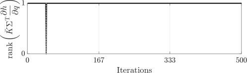
(a)

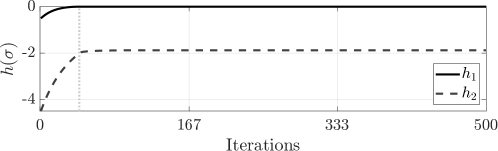
(b)

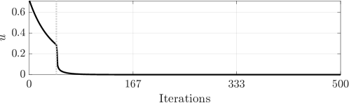
(c)

Figure 2: Simulation of the scenario presented in Example 4 to show the effects of the loss of rank of the matrix $\mathrm{rank}\left(\bar{K}\Sigma^{\sf T}\dfrac{\partial h}{\partial q}\right)$. Figure 2a shows the rank evaluated, as explained in Example 4, during the course of the simulation. Despite the loss of rank happening at iteration 44 (vertical dotted line), Figures 2b and 2c show that both the task functions $h_{1}$, $h_{2}$, and the robot input $u$ are continuous.

Remark 10 ((Parameter tuning)).

As discussed in Section 3.1 and confirmed in this section through Proposition 6, the choice of prioritization matrix $K$ does not influence the feasibility or the convergence of the prioritized execution of a stack of tasks. Nevertheless, the way tasks are accomplished depends on the parameters of $K$. In Section 3.2, a natural way of automatically selecting a prioritization constraint is shown. As a result, compared to the execution of multiple prioritized Jacobian-based tasks, using ESB tasks does not require a careful choice of parameters to ensure the convergence of the task variables to zero.

4 Planning of Switching Task Prioritizations

In the previous section, we proved the stability of executing multiple ESB tasks in a prioritized fashion. This section illustrates an algorithm to reorder priorities among ESB tasks during their execution. In particular, Proposition 7 presents a stack transition method which consists in weighting the control inputs $u_{1}$ and $u_{2}$ corresponding to the execution of two stacks prioritized by the prioritization matrices $K_{1}$ and $K_{2}$, respectively, in order to transition between them. The same approach is applicable to the case where priorities are enforced using the adaptive prioritization matrix approach as in Section 3.2.

Proposition 7.

Let $u_{1}$ and $u_{2}$ be the control inputs corresponding to the execution of the stacks of tasks prioritized by the prioritization matrices $K_{1}$ and $K_{2}$. Let the robot execute the control input

$$u=s(t)u_{1}+(1-s(t))u_{2}$$ (64)

in the time interval $t\in[0,T]$, where $s(t)=1-\frac{t}{T}$. Then, the transition from executing the stack of tasks with prioritization matrix $K_{1}$ to $K_{2}$ is continuous.

Moreover, at each time instant $t\in[0,T]$, relative priorities that do not change in the initial and final prioritized stack are maintained throughout the switching time interval.

Proof.

Continuity of the controller $u$ in (64) follows from the continuity of $u_{1}$, $u_{2}$ (as shown in [NMS⁺20]), and $s(t)$.

It remains to show that the relative priority between tasks, whose relative priority remains unchanged, is kept during the transition. To this end, recalling that the component of $\gamma_{0}(h)$ is different from zero when the corresponding $i$-th task is not fully completed, from Proposition 6, it follows that when tasks are not completed, one has that

$$\frac{\partial h}{\partial x}u(t)+\gamma(h)=\delta(t)$$ (65)

for $u(t)$ and $\delta(t)$ solutions of the optimization program (29) at time $t$.

Then, by the definitions of $u_{1}$ and $u_{2}$, one can write:

$$\frac{\partial h}{\partial x}u+\gamma(h)$$ (66)

$$= \frac{\partial h}{\partial x}\big{(}s(t)u_{1}+(1-s(t))u_{2}\big{)}+\gamma(h)$$

$$= s(t)\left(\frac{\partial h}{\partial x}u_{1}+\gamma(h)\right)(1-s(t))\left(\frac{\partial h}{\partial x}u_{2}+\gamma(h)\right)$$

$$= s(t)\delta_{1}+(1-s(t))\delta_{2}=:\Delta,$$

where $\Delta$ is defined to be the convex combination of $\delta_{1}$ and $\delta_{2}$. It is assumed that $K_{1}\delta_{1}\geq 0$ and $K_{2}\delta_{2}\geq 0$. If task $T_{i}\prec T_{j}$ in both stacks, then

$$\delta_{1,i} <\delta_{1,j}$$ (67)

$$\delta_{2,i} <\delta_{2,j},$$

then

$$\Delta_{i}(t) =s(t)\delta_{1,i}+(1-s(t))\delta_{2,i}$$ (68)

$$<s(t)\delta_{1,j}+(1-s(t))\delta_{2,j}=\Delta_{j}(t),$$

which means that the relative priority between tasks, whose relative priority does not change between initial and final stacks, remains unchanged throughout the transition. ∎∎

Remark 11 ((Minimal invasivity of input-based stack transition)).

As a result of Proposition 7, the input-based stack transition is minimally invasive in the stack transition in the sense that only the tasks that change their position in the final prioritization stack with respect to the initial one are affected during the switching phase.

Besides the amenable minimal invasivity property discussed in the previous remark, another important property of this priority stack switching approach is the resulting stability guarantees on the execution of the prioritized stacks of tasks, as highlighted in the following proposition.

Proposition 8.

Consider a robot executing a stack of tasks characterized by the prioritization matrix $K_{1}$ for $t<0$. In the time interval $t\in[0,T]$, the initial stack is switched to the one characterized by the prioritization matrix $K_{2}$, using the control input (64), where

$$\begin{cases}s(t)\equiv 1\quad&\forall t\leq 0\\ s(t)\in[0,1]\quad&t\in[0,T]\\ s(t)\equiv 0\quad&\forall t\geq T\end{cases}$$ (69)

Assuming $\gamma$ is continuously differentiable, and the CBFs encoding the ESB tasks have bounded derivatives, then for $z_{2}$ defined (similarly to (55)) as

$$z_{2}=\bar{K}_{2}\Sigma_{2}^{\sf T}\gamma(h),$$ (70)

one has that $z_{2}(t)\to 0$ as $t\to\infty$.

Proof.

Let us start by considering the dynamics of $z_{2}$ resulting from the application of the input (64) required to switch prioritized stack:

$$\dot{z}_{2} =\underbrace{\bar{K}_{2}\Sigma_{2}^{\sf T}\frac{\partial\gamma}{\partial h}\frac{\partial h}{\partial q}}_{=:\Psi_{2}(q)}\dot{q}$$ (71)

$$=\underbrace{\Psi_{2}(q)s(t)}_{B(q,t)}\underbrace{\dot{q}_{1}^{\star}}_{=:w}+\underbrace{\Psi_{2}(q)(1-s(t))\dot{q}_{2}^{\star}}_{=:(1-s(t))f_{\text{cl}}(q)}$$

$$=(1-s(t))f_{\text{cl}}(q)+B(q,t)w,$$

where $\dot{q}_{1}^{\star}$ and $\dot{q}_{2}^{\star}$ are the solutions of (29) with $K$ equal to $K_{1}$ and $K_{2}$, respectively.

Consider the Lyapunov function $V(z_{2})=\frac{1}{2}\|z_{2}\|^{2}$ defined as in (56). Proposition 6 shows that $V$ is a Lyapunov function for the zero-input system

$$\dot{z}_{2}=(1-s(t))f_{\text{cl}}(q),$$ (72)

owing to the properties of $s(t)$ in (69).

Now, using the results of Proposition 6, let us evaluate the time derivative of $V$ along the trajectories of the system (71):

$$\dot{V} \leq-(1-s(t))V(z_{2})+z_{2}^{\sf T}B(q,t)w$$ (73)

$$=-(1-s(t))\frac{1}{2}\|z_{2}\|^{2}+z_{2}^{\sf T}B(q,t)w$$

$$=-\frac{1}{2}(1-s(t))(1-\lambda)\|z_{2}\|^{2}-\frac{1}{2}(1-s(t))\lambda\|z_{2}\|^{2}$$

$$\quad+z_{2}^{\sf T}B(q,t)w$$

$$\leq-\frac{1}{2}(1-\lambda)\|z_{2}\|^{2}-\frac{1}{2}\lambda\|z_{2}\|^{2}+z_{2}^{\sf T}B(q,t)w,$$

where the last inequality holds for $t>0$, i.e., when the priority switch happens.

From the properties of the function $s(t)$ stated in (69), and by the assumption that the CBFs encoding the tasks have bounded derivatives, one has that $B(q,t)$ is uniformly bounded. Therefore, we can upper bound $\dot{V}$ as follows:

$$\dot{V} \leq-\frac{1}{2}(1-\lambda)\|z_{2}\|^{2}-\frac{1}{2}\lambda\|z_{2}\|^{2}+\|z_{2}\|\|B\|\|w\|$$ (74)

$$-\frac{1}{2}(1-\lambda)\|z_{2}\|^{2}-\frac{1}{2}\lambda\|z_{2}\|\left(\|z_{2}\|-2\frac{\|B\|\|w\|}{\lambda}\right)$$

$$\leq-\frac{1}{2}(1-\lambda)\|z_{2}\|^{2},$$

for all $\|z_{2}\|\geq\frac{2\|B\|}{\lambda}\|w\|$. This condition shows that $V$ is an ISS-Lyapunov function for (71) ([Son08]). By Corollary 2.2 in [ELW00], the system (71) is input-to-state stable, i.e., there exist a class $\mathcal{K}\mathcal{L}$ function $\beta$ and a class $\mathcal{K}$ function $\chi$ such that:

$$\|z_{2}(t)\|\leq\beta\left(\|z_{2}\|,t\right)+\chi\left(\max_{0\leq\tau\leq t}\|w(\tau)\|\right).$$ (75)

Hence, $\|z_{2}(T)\|<\infty$, and, by Proposition 6, $z_{2}(t)\to 0$ as $t\to\infty$. ∎∎

This proposition shows that, under mild assumptions (bounded derivative) on the CBFs encoding the ESB tasks to execute, the switch between two prioritized stacks of tasks can be executed without compromising the stability of the robotic system. This will be highlighted in the simulations and experiments reported in Section 6.

So far, we considered only velocity-controlled robots. Nevertheless, in many practical applications, having the ability of controlling the joint torques is required. The next section is devoted to the specialization of the proposed prioritized task execution framework to torque-controlled robotic systems, accounting, in particular, for the presence of torque bounds.

5 Extended Set-based Task Execution with Torque Bounds

In the previous sections, we analyzed the execution of multiple prioritized tasks using a kinematic model of robotic manipulators where there is a nonlinear single-integrator relation—given by (5)—between the velocity in the task space and the velocity in the joint space. In this section, we extend the approach developed so far to robot dynamic models.

5.1 Dynamic Model

In task-prioritized control of robotic manipulators executing highly dynamic tasks—i.e., tasks requiring large accelerations, so that the effects of robot inertia are not negligible anymore—the following robot dynamic model is typically employed:

$$D(q)\ddot{q}+C(q,\dot{q})\dot{q}+F_{v}\dot{q}+g(q)=\tau,$$ (76)

where $q$ are the joint angles, $D(q)$ is the inertia matrix, $C(q,\dot{q})$ accounts for centrifugal and Coriolis effects, $F_{v}\dot{q}$ models viscous friction (static friction is neglected), $g(q)$ is the effect of gravity, and $\tau$ is the vector of joint input torques (see, e.g., [SHV⁺06] or [SSVO10]).

The control affine model introduced in (7) is amenable to capture also the dynamics of robotic manipulators. For the remainder of this section, we let the state of the robot modeled by (76) be denoted by $x=[q^{\sf T},\dot{q}^{\sf T}]^{\sf T}$, so that (76) can be written in the control affine form (7) with

$$f(x)=\begin{bmatrix}\dot{q}\\ -D^{-1}(q)\big{(}C(q,\dot{q})\dot{q}+F_{v}\dot{q}+g(q)\big{)}\end{bmatrix}$$ (77)

and

$$g(x)=\begin{bmatrix}0\\ D^{-1}(q)\end{bmatrix}.$$ (78)

Without loss of generality, in this section we only consider ESB tasks which do not depend explicitly on time. A task $T_{i}$, defined in terms of the task variable $\sigma_{i}$ via the CBF $h_{i}(\sigma_{i})$, can be executed by enforcing the constraint

$$\dot{h}_{i}(\sigma_{i},x,u)+\gamma(h_{i}(\sigma_{i}))$$ (79)

$$= \frac{\partial h_{i}}{\partial\sigma_{i}}\frac{\partial\sigma_{i}}{\partial x}f(x)+\frac{\partial h_{i}}{\partial\sigma_{i}}\frac{\partial\sigma_{i}}{\partial x}g(x)u+\gamma(h_{i}(\sigma_{i}))\geq 0.$$

If

$$\frac{\partial h_{i}}{\partial\sigma_{i}}\frac{\partial\sigma_{i}}{\partial x}g(x)=0,$$ (80)

then the CBF $h_{i}$ is said to have relative degree higher than 1. At this point, one could make use of exponential CBFs ([NS16]) or, more generally, define the following auxiliary CBF (as in [NE21]):

$$h_{i}^{\prime}(\sigma_{i},x)=\dot{h}_{i}(\sigma_{i},x)+\gamma_{i}(h_{i}(\sigma_{i})),$$ (81)

and then enforce the following condition analogous to (LABEL:eq:cbfineqtask):

$$\dot{h}^{\prime}_{i}(\sigma_{i},x,u)+\gamma(h^{\prime}_{i}(\sigma_{i}))\geq 0,$$ (82)

where the term $\dot{h}^{\prime}_{i}(\sigma_{i},x,u)$ explicitly depends on $u$ as the dynamical system (76) is a second-order system.

In general, we define $h_{i}^{\prime}$ to be:

$$h^{\prime}_{i}(\sigma_{i},x)=\begin{cases}h_{i}(\sigma_{i})&\text{ if $h_{i}$ has relative degree 1}\\ \text{Eq.}~{}\ref{eq:hiprime}&\text{ if $h_{i}$ has relative degree 2},\end{cases}$$ (83)

and solve the following optimization problem to synthesize the controller (i.e., joint torques) required to execute a prioritized stack of tasks:

$$\operatorname*{minimize~{}}_{u,\delta} \|u\|^{2}+l\|\delta\|^{2}$$ (84)

$$\operatorname*{subject\,to~{}} \frac{\partial h^{\prime}_{i}}{\partial\sigma_{i}}\frac{\partial\sigma_{i}}{\partial x}f(x)+\frac{\partial h^{\prime}_{i}}{\partial\sigma_{i}}\frac{\partial\sigma_{i}}{\partial x}g(x)u$$

$$+\gamma\prime_{i}(h^{\prime}_{i}(\sigma_{i}))\geq-\delta_{i}\quad\forall i\in\{1,\ldots,M\}$$

$$K\delta\leq 0.$$

5.2 Actuation Constraints

The solution to (84) may not be physically implementable in the presence of torque bounds, which are expressed as box constraints on the input optimization variable $u$. However, if one attempts to solve (84) with the additional constraint

$$\|u\|_{\infty}\leq u_{\mathrm{max}}<\infty,$$ (85)

tasks might not be executed as desired, as the optimal control input solution to the optimization program results in large relaxation variables $\delta$. The problem becomes even more serious when multiple safety-critical constraints are present. In fact, by definition, safety-critical constraints should not be relaxed, and, if more than one such constraint is present, the optimization program might be infeasible.

Actuation constraints in multi-task execution have been considered already in the context of Jacobian-based tasks. The so-called task scaling procedure was designed to slow down the execution of the task by scaling down joint velocities and accelerations not to exceed the maximum allowed values. However, as a result, the task execution performance may be degraded. Several approaches to this problem have been proposed (see, e.g., [FBP20] or [LKCK22] for recent solutions). In [FDK15], the authors present an algorithm to select the least possible task-scaling in order to control redundant manipulators in presence of hard joint constraints, in terms of joint positions, velocities, and accelerations.

A constraint-based control strategy for multi-task execution has been presented in [BP20], where the authors consider the robot dynamic model (76) and include torque bounds in the optimization program required to evaluate the input torques to execute the robotic tasks. Nevertheless, a formal analysis on the quality of task execution in presence of input bounds is lacking. Relaxation variables allow the optimization program to remain feasible at the cost of degrading the performance of task execution, similarly to the task scaling procedure mentioned above.

In this paper, we built upon the CBF-based method proposed in [ANWE20] to account for input bounds. The solution consists in dynamically extending a system in order to turn the input vector into a state and be able to enforce input constraint using integral CBFs, by treating them as state constaints. However, the main result in [ANWE20] hinges on the feasibility of the formulated QP, which is not guaranteed. Thus, a careful parameter choice has to be made in order to ensure the feasibility of the optimization program at each point in time during online operations.

In this section, we present a systematic approach to find the best possible choice of parameters which are able to ensure that the optimization program defined to synthesize the controller value will always remain feasible, even in presence of input bounds and multiple safety-critical tasks. This will be achieved without degrading the performance of task execution via relaxation variables.

More specifically, the problem of the feasibility of the task execution in presence of input bounds can be solved by an appropriate choice of the class $\mathcal{K}$ functions $\gamma_{i}$ used to define $h_{i}^{\prime}$ in (81). In the following, we consider linear class $\mathcal{K}$ functions, namely

$$\gamma_{i}(s)=\Gamma_{i}s,$$ (86)

with $\Gamma_{i}>0$ for all $i$. The problem now becomes that of finding values of the parameters $\Gamma_{i}$ so that (76) is always feasible, even in presence of multiple safety-critical tasks and/or input bounds. This objective can be cast as the following semi-infinite program:

$$\operatorname*{maximize~{}}_{u,\Gamma_{1},\ldots,\Gamma_{M}} \sum_{i=1}^{M}\Gamma_{i}$$ (87)

$$\operatorname*{subject\,to~{}} \dot{h}_{i}^{\prime}(\sigma_{i},x,u,\Gamma_{i})\geq 0$$

$$\|u\|_{\infty}\leq u_{\mathrm{max}}$$

$$\Gamma_{i}\geq 0$$

$$\qquad\forall x\in\cup_{j\in\{1,\ldots,M\}}\big{\{}x\in\mathbb{R}^{n_{x}}\colon h^{\prime}_{j}(\sigma_{j}(x))=0\big{\}}$$

$$\qquad\forall i\in\{1,\ldots,M\}.$$

The maximization is justified by the fact that we aim at finding the largest possible approximation of the feasible set which is affine in $\Gamma_{i}$ and hence its size grows with $\Gamma_{i}$. The reason to apply the constraints $\dot{h}_{i}^{\prime}(\sigma_{i},x,u,\Gamma_{i})\geq 0$ only on the union of the boundaries of the zero superlevel sets of the functions $h^{\prime}_{i}(\sigma_{i})$ follows from Nagumo’s theorem ([Nag42]). This allows us to significantly reduce the complexity of solving (87). The latter, moreover, despite being a semi-infinite program, can be computed offline only once in order to obtain optimal values of the parameters $\Gamma_{i}$. To summarize, employing the $\Gamma_{i}$ solution of (87) in the definition of $h^{\prime}_{i}$ in (83) has two beneficial effects:

1. Tasks need not be relaxed because of torque bounds

2. The task prioritization and execution optimization program. (84) is always feasible even in presence of multiple safety-critical constraints and torque bounds.

Example 5 ((Task execution with torque bounds)).

Let us compare the behavior of a dynamic robotic manipulator executing an ESB task with input saturation and with integral CBFs, respectively. The ESB task consists in driving the end-effector of a 3-link serial manipulator to a desired configuration in the Cartesian space. As a consequence of the fact that there are no joint speed constraints, the solution of (87) in terms of $\Gamma_{i}$ is unbounded above, i.e., an arbitrarily high value of $\Gamma_{i}$ can be chosen in the definition of $h_{i}^{\prime}$,

Using torque saturation

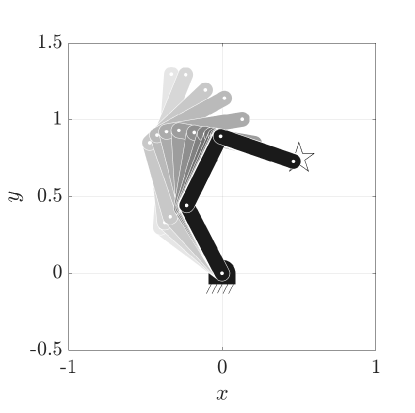
(a)

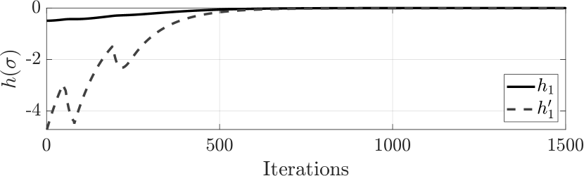
(b)

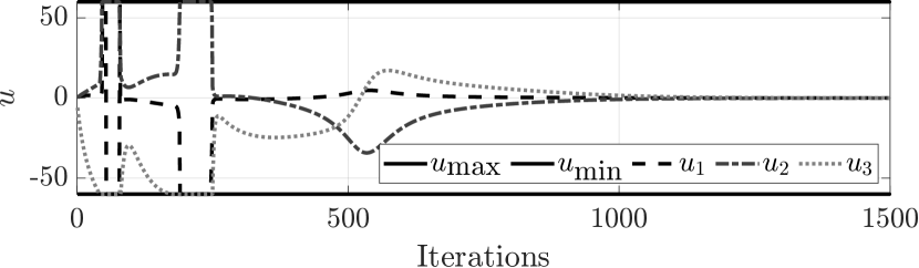
(c)

Using CBFs on torque inputs

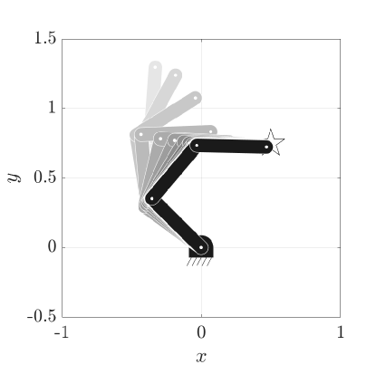
(d)

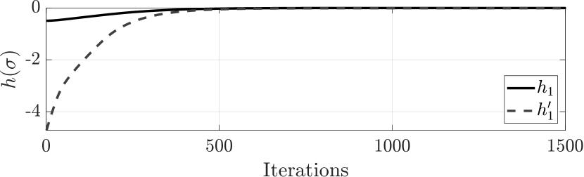
(e)

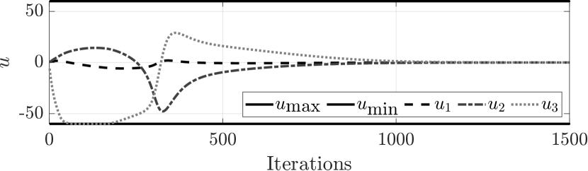
(f)

Figure 3: Enforcing torque bounds using a posteriori saturation vs CBFs on torque input. When saturating torque values, the maximum/minimum torques were set to $\pm 60$ Nm to make the simulation of the saturated controller stable. On the contrary, using integral CBFs never compromises the stability of the task execution. Furthermore, torques computed using the QP (84) with additional integral CBFs to enforce torque bounds are much smoother compared to those achieved via saturation. This is a desirable property when dealing with torque-controlled robots as it avoids higher order effects which might compromise the stability of the robot.

Figure 3 reports the results of two simulations performed saturating input torques after solving the optimization program (84) (Figures 3a, 3b, and 3c), and enforcing input constraints and task execution constraints holistically using CBFs and integral CBFs, as described in this section (Figures 3d, 3e, and 3f). First of all, it is important to mention that the value of the maximum torque (60 Nm) was chosen so to make the simulation of the saturated controller stable. Using integral CBFs, the stability of the task execution itself is never compromised by a maximum value of the input torque.

A second advantage of using the approach described in this section over an a posteriori saturation of the input torques is visible when comparing Figs. 3c and 3f. The time evolution of the torques is generally smoother when CBFs are used compared to the torque saturation approach. This is a desirable behavior when dealing with torque-controlled robots as an abrupt change in the torque value may introduce higher order effects which, in turn, may compromise the stability of the robotic system.

6 Simulations and Experiments

In this section, we present the results of simulations and experiments performed to showcase the behavior of a robot manipulator executing multiple prioritized tasks controlled using the proposed framework. The execution of three independent tasks is shown in Section 6.1, while three dependent prioritized tasks are considered in Section 6.2. Sections 6.3 and 6.4 illustrate the switching behavior between tasks of the same nature and of different nature, respectively. Section 6.5 deals with prioritized tasks executed by a torque-controlled robot, and the results of the implementation of the presented framework on the KUKA LBR iiwa 7 R800 manipulator robot is presented in Section 6.6.

The robot considered in the simulations in Sections 6.1-6.5 is a planar three-link three-revolute-joint open kinematic chain. The length of each of the links is 0.5m. The task functions are defined following Example 1 where, for each task, $\sigma_{d}$ is a constant in time.

6.1 Execution of independent tasks

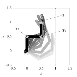
(a)

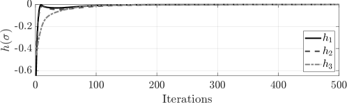
(b)

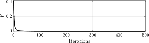
(c)

Figure 4: Execution of 3 independent tasks using the method in Section 3.1.Each task consists in driving the endpoint of link $i$ to the position labeled as $T_{i}$ and marked with a star. Figure 4a shows the evolution of the configuration of the robot (from light gray to black). Figures 4b and 4c show the evolution of the task functions $h_{i}$ and the Lyapunov function $V$ in (56), respectively. As can be seen the task functions converge to zero, as does the Lyapunov function, since all tasks are independent.

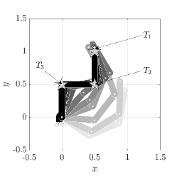
(a)

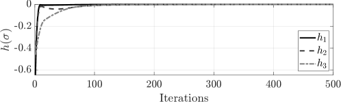
(b)

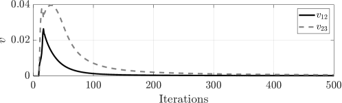
(c)

Figure 5: Execution of 3 independent tasks using the method in Section 3.2. Each task consists in driving the endpoint of link $i$ to the position labeled as $T_{i}$ and marked with a star. Figure 5a shows the evolution of the configuration of the robot (from light gray to black). Figures 5b and 5c show the evolution of the task functions and of the components of the slack variable $v$ of the prioritization constraint, respectively.

This section considers the execution of independent tasks, consisting in controlling the endpoints of each of the three links to reach a desired position in the plane compatible with the geometry of the robot. The three desired positions, depicted as as stars in Fig. 4, are $\sigma_{1}=[0.5,\,1]^{\sf T}$, $\sigma_{2}=[0.5,\,0.5]^{\sf T}$, $\sigma_{3}=[0,\,0.5]^{\sf T}$, respectively. By Proposition 2, these three ESB tasks are independent as their corresponding Jacobian-based tasks are independent.

As per Corollary 1, all the tasks will be executed regardless of their relative priorities. To compare the behavior of the robot executing tasks with a pre-specified stack (as in Section 3.1) with the automatic task prioritization (as in Section 3.2), two simulations are performed. The results of the first one are reported in Fig. 4. Here the robot is controlled by the optimal input computed by solving QP (29), with a fixed prioritization stack. By Corollary 1, all tasks are executed as shown in Figures 4a and 4b, and the Lyapunov function in (56) converges to zero (Fig. 4c). It is worthwhile noting that, due to task independence, all functions $h_{i}$ for $i=1,\,2,\,3$ converge to zero, demonstrating the accomplishment of all the tasks as expected.

While the behavior in Fig. 4 is obtained by letting the robot execute the optimal control input solution to the QP (29), in Fig. 5 the robot fulfills the same task by executing the solution to the QP (30). In this case, following the motivation given in Section 3.2, i.e., assuming we do not know whether the designed tasks are independent, we relax the prioritization constraint. The behavior of the robot is shown qualitatively in Fig. 5a and quantitatively in Fig. 5b. These figures demonstrate how, despite the prioritization constraint relaxation, the robot executes all three tasks, as desired. In Fig. 5c, we report the plot of the slack variables—two components of the vector $v$ in (30)—which relax the prioritization constraint. As can be seen, the optimization program initially relaxes the prioritization constraints (higher $\|v\|^{2}$ at the beginning of the simulation), which are asymptotically tightened ($\|v\|^{2}\to 0$ as the simulation iterations increase), effectively realizing the stack prescribed by $K$ in (30).

6.2 Execution of dependent tasks

In this section, we consider dependent tasks. As pointed out in Section 3.2, the approach with a fixed prioritization matrix might not lead to a convergent behavior if the prioritization matrix defining the stack of tasks is not designed respecting the geometry of the tasks themselves. Therefore, for the case of dependent tasks the robot is controlled using the QP (30), where the prioritization constraint is relaxed.

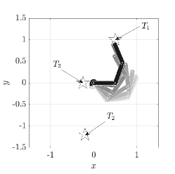
(a)

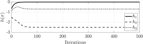
(b)

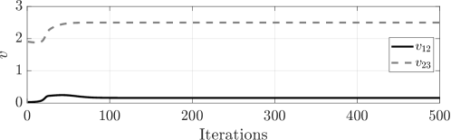
(c)

Figure 6: Execution of 3 dependent tasks consisting in driving the end-effector of the robot to each of the 3 points marked with a star. As in previous simulations, the evolution of the robot configuration is depicted in Fig. 6a. The robot executes task $T_{1}$ since it has highest priority and all tasks are pairwise dependent. As a result, in Fig. 6b, only $h_{1}$ is driven towards 0, signifying the execution of task $T_{1}$ only. Figure 6c depicts the components of the slack variable $v$ of the prioritization constraint.

The three dependent tasks defined in this simulation consist in controlling the end-effector (the endpoint of the third link) of the robot to reach three predefined positions in the plane. The three desired positions, depicted as stars in Fig. 6, are $\sigma_{1}=[0.5,\,1]^{\sf T}$, $\sigma_{2}=[-0.2,\,-1.2]^{\sf T}$, $\sigma_{3}=[-0.25,\,0]^{\sf T}$, respectively. The tasks are dependent according to Definition 8. In fact, it is not hard to see that there exists a configuration of the robot for which the gradients of the two tasks are aligned.

Proposition 6 shows that the tasks must converge to the set (50), corresponding to the condition in which all tasks with active constraints are executed respecting their relative priorities. The prescribed prioritization stack is $T_{1}\prec T_{2}\prec T_{3}$, with corresponding prioritization matrix equal to

$$K=\begin{bmatrix}1&-1/\kappa&0\\ 0&1&-1/\kappa\end{bmatrix},$$ (88)

where $\kappa=10^{3}$. With this choice of $\kappa$ and $\sigma_{i}$, the desired relative priorities are not realizable—because of geometric reasons. Thanks to the prioritization constraint relaxation, however, the QP (30) finds the closest prioritization stack that is realizable by the robot.

The results are shown in Fig. 6. In particular, Fig. 6a depicts the time evolution of the robot configuration, which clearly executes task $T_{1}$ with highest priority, by moving its end-effector to the point marked with a star and labeled as $T_{1}$. The corresponding task functions $h_{i}$ for $i=1,\,2,\,3$ are reported in Fig. 6b, where it is possible to see how $h_{1}(\sigma(t))\to 0$ as the simulation iterations increase, while $h_{2}(\sigma(t))$ and $h_{3}(\sigma(t))$ converge to finite values different from 0—corresponding to the non-accomplishment of tasks $T_{2}$ and $T_{3}$. In fact, due to task dependence, not all the values of the functions $h_{i}$ can converge to zero, i.e., intuitively the three tasks cannot be accomplished simultaneously.

Figure 6c shows the plot of the slack variables of the prioritization stack constraint. As expected, their values does not converge to zero, as the prioritization constraint prescribed by (88) is not geometrically realizable.

6.3 Switching between dependent tasks

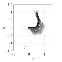
(a)

(b)

(c)

(d)

(e)

Figure 7: Priority switching with dependent tasks consisting in driving the end-effector of the robot to each of the 3 points marked with a star. Figures 7a, 7b and 7c show the configuration of the robot (evolving from light gray to black in each figure) while it executes task $T_{1}$, $T_{2}$, and $T_{3}$ with highest priority, respectively. Figure 7d reports the trajectories of the task functions $h(\sigma)$. Light gray shaded areas denote the intervals during which priorities are swapped. In the first segment (left of the first light gray shaded area), task $T_{1}$ has highest priority. Correspondingly, $h_{1}$ is driven to zero. Then, $T_{1}$, $T_{2}$ priorities are swapped. Analogous behavior can be observed in the second interval where $h_{2}$ is driven to zero. After that, priorities are swapped again ($T_{3}$ acquires highest priority) and the third interval shows convergence of $h_{3}$ to zero. Finally, Fig. 7e shows how the joint velocity control input evaluated by solving the QP (30) is continuous even during the switch of priority stacks.

In this and the next sections, we switch our focus to dynamic prioritization stacks where the relative priorities between tasks change over time, and show the behavior of the kinematic and dynamic robot models under the control framework presented in Section 4.

In this section, we consider the same tasks of the previous example, which consist in reaching predefined positions in the task space with the robot end-effector. As before, the three desired positions are $\sigma_{1}=[0.5,\,1]^{\sf T}$, $\sigma_{2}=[-0.2,\,-1.2]^{\sf T}$, $\sigma_{3}=[-0.25,\,0]^{\sf T}$, respectively, resulting in dependent tasks. Their relative priorities change according to the following sequence of stacks:

$$\begin{cases}T_{1}\prec T_{2}\prec T_{3}&0\leq\text{Iteration}<3333\\ T_{2}\prec T_{3}\prec T_{1}&3333\leq\text{Iteration}<6666\\ T_{3}\prec T_{1}\prec T_{2}&6666\leq\text{Iteration}<10000.\end{cases}$$ (89)

Figure 7 shows data recorded during the simulation. In particular, Figures 7a–7c depict the motion of the robot executing the tasks prioritized based on the three stacks specified in (89), respectively. As can be seen, the robot moves sequentially to the point corresponding to the task with highest priority. Figure 7d shows the time evolution of the task functions $h_{i}$ for $i=1,\,2,\,3$. Notice how the value of the function corresponding to the task with highest priority always converges to a value close to zero. Finally, Fig. 7e shows the robot input $u=\dot{q}$, highlighting its continuity during the switching phases.

6.4 Insertion and removal of dependent and independent tasks

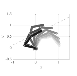
(a)

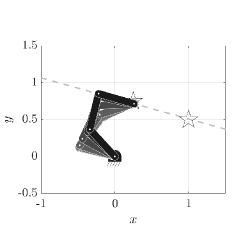
(b)

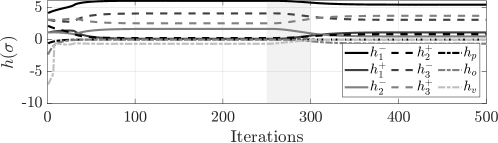
(c)

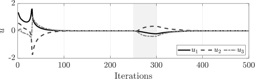
(d)

Figure 8: Task insertion/removal and switch between stacks of dependent tasks. The tasks considered in this simulations are joint limit avoidance, end-effector position control, end-effector orientation control, and a look-at-point task in which we control the third link of the robot to the orientation required to aligned it with a desired point of interest. The orientation control and the look-at-point tasks are dependent, and the switch consists in removing the orientation control task and inserting the look-at-point task. Figures 8a and 8b show the evolution of the robot configurations while executing the two stacks of tasks, respectively. The stars represent the desired end-effector position and the point towards which the third link has to be oriented. The plot of the task functions are reported in Fig. 8c, while Fig. 8d highlights the continuity of the joint velocity control input evaluated by solving the QP (30) during the switching phase between stacks of tasks. Light gray shaded area denote the interval in which priorities are swapped.

In this final simulation performed using the kinematic robot model, we demonstrate how the proposed framework can not only handle time-varying prioritization stacks, but also allows for insertions and removals of tasks in and from a stack being executed. To better illustrate the task insertion/removal capability, in this section we consider tasks of different nature, consisting in remaining within the physical joint limits and orienting the end-effector towards a desired point of interest. The desired end-effector position is $\sigma=[0.25,\,0.75]^{\sf T}$, the desired orientation of the end-effector is $\sigma=\pi/6$, the point to monitor is at $\sigma=[1,\,0.5]^{\sf T}$. The joint angle upper and lower bounds are set to $q^{+}=[\pi,\,2/3\pi,\,2/3\pi]^{\sf T}$, $q^{-}=[-\pi,\,-2/3\pi,\,-2/3\pi]^{\sf T}$, respectively. Staying within joint limits is the highest priority task, reaching the desired position is the secondary task, and orientation and look-at-point tasks are the lowest-priority tasks.

The simulation is divided into two parts and the switch between task stacks happens in the interval $[250,300]$ iterations. In the first part, the robot has to reach desired position and orientation with its end-effector while staying within joint limits. In the second part, a look-at-point task replaces the orientation task, thus resulting in task removal and insertion. The transition between the task stacks is implemented using the approach in Proposition 7.

Figure 8 shows data recorded during the simulation. In Figs. 8a and 8b, the motion of the robot executing the two stacks of tasks, respectively, is depicted. The stars represent the desired end-effector position and the point of interest towards which the third link has to be oriented. The gray dashed lines passing through the desired end-effector position denote the desired orientation direction in Fig. 8a and the direction pointing towards the point of interest in Fig. 8b. Figure 8c shows the time evolution of the task functions, where $h_{i}^{+}$, $h_{i}^{-}$ denote the upper and lower $i$-th joint limit task, respectively. The functions $h_{p}$, $h_{o}$, $h_{v}$ denote the position, orientation and vision task CBF functions, defined as in Example 1. Finally, we show that the robot inputs $u=\dot{q}$ in Fig. 8d, to highlight its continuity during the stack switch and task insertion/removal operations.

6.5 Switching between dependent tasks (dynamic model)

In the previous sections we employed kinematic models of manipulator for the control synthesis. The simulation presented in this section aims at showcasing the proposed task prioritization framework applied to the case of dynamic robot models, controlled using joint torque inputs.

The robot is the same 3-link serial manipulator considered in the previous sections and it is modeled by (76). Similar to the previous examples, the two tasks to be executed in a prioritized fashion consist in regulating the end-effector to two different locations in the plane. Thus, they are dependent according to Definition 8.

As discussed in Section 5, when dynamic models are considered, we need to define the auxiliary CBF $h_{i}^{\prime}$, as in (83). In addition, in this section input constraints are enforced by dynamically extending the model (76) as follows:

$$\begin{cases}\dot{x}=f(x)+g(x)u\\ \dot{u}=u^{\prime},\end{cases}$$ (90)

where $x$, $u$, $f$, and $g$ are defined in Section 5, $u$ becomes part of the state, and $u^{\prime}$ is the new input to the dynamical system. Proceeding as in [ANWE20], the following integral CBF is defined

$$h_{u}(u)=u_{\mathrm{max}}^{2}-\|u\|^{2},$$ (91)

and the constraint $\dot{h}_{u}(u,u^{\prime})+\gamma_{u}(h_{u}(u))\geq 0$ is enforced to keep the magnitude of the input torques within the desired bound.

(a)

(b)

(c)

(d)

Figure 9: Priority switching with dependent tasks and torque-controlled robot. Similarly to its kinematic counterpart in Fig. 7, Figures 9a and Figures 9b show the evolution of the robot configurations. In Fig. 9c, instead, besides the trajectory of $h_{1}$ and $h_{2}$, the functions $h_{1}^{\prime}$ and $h_{2}^{\prime}$ are displayed. In the first half of the experiment, task $T_{1}$ has highest priority: consequently, $h_{1}$ and $h_{1}^{\prime}$ are driven to zero. Analogously, in the second half of the experiment, the priorities are swapped and $h_{2}$ and $h_{2}^{\prime}$ are driven to zero by the optimal torques solution of (84). Finally, Fig. 9d, the continuity of the input torques required to switch between the two stacks of tasks is shown, alongside the minimum and maximum values they can attain.

Figure 9 shows the result of the execution of the two prioritized tasks, whose priority is swapped half way through the experiment. In particular, Figs. 9a and 9b show the motion of the robot while executing the prioritized stacks $T_{1}\prec T_{2}$ and $T_{2}\prec T_{1}$, respectively. The positions to which the end-effector is to be regulated are depicted as stars: the top position corresponds to task $T_{1}$, while controlling the end-effector to the bottom position is equivalent to executing task $T_{2}$. The values of the CBFs $h_{1}$, $h_{2}$, $h_{1}^{\prime}$, and $h_{2}^{\prime}$ used to execute the two tasks are plotted in Fig. 9c. As can be seen, the CBFs corresponding to the task executed with highest priority are driven to zero. Finally, the joint torques, $u$, obtained by integrating $u^{\prime}$ in (90) and used to control the robot, are reported in Fig. 9d, where we observe that torques are continuous during the priority switch. Furthermore, the torque values, depicted as thick black lines, never exceed the upper and lower bounds, $u_{\mathrm{max}}=60$ Nm.

6.6 Robot experiments

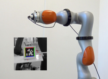
Figure 10: Experimental setup. The KUKA LBR iiwa 7 R800 robot equipped with a RealSense T435 camera at its end-effector. The superimposed picture shows the camera image overlayed with Aruco tag tracking marks.

To further validate the methods introduced in this paper, in this section we present the results of experiments performed on a real 7-DOF anthropomorphic manipulator. We show how the proposed framework effectively executes and prioritizes a time-varying task stack. comprised by both dependent and independent ESB tasks as well as safety-critical tasks.

The experimental setup consists of the KUKA LBR iiwa 7 R800 robot with a RealSense T435 camera mounted on its tip (see Fig. 10). The control algorithm runs on a laptop with an Intel Core i7 processor and $16$ Gb RAM. The manipulator is torque-controlled with a Fast Robot Interface (FRI) client application (see [SSB10]) that communicates with the robot through an Ethernet connection link, and runs with a command sending period of $T_{cmd}=0.3$ ms. The torque $\tau_{\text{FRI}}\in\mathbb{R}^{7}$, used to track the desired joint positions and velocities, is computed as follows:

$$\tau_{\text{FRI}}(t)=k_{u}\,(u(t)-\dot{q}(t))+k_{q}\,(q_{d}(t)-q(t)),$$ (92)

where $u\in\mathbb{R}^{7}$ is obtained solving the QP (30), $q_{d}$ by integrating the desired joint velocities $u(t)$, and the control gains were chosen to be $k_{u}=100$ and $k_{q}=36$. The QP is solved online in a ROS node employing the OSQP library [SBG⁺20], and evaluating the CBFs using measured joint positions $q$. A middle-layer ROS node acts as an interface between ROS and the FRI client application.

To better illustrate the performance of the proposed framework on a real robot, we consider tasks of different nature and which are dynamically inserted and removed in the prioritized stack. The following ESB tasks are employed to perform position control: (i) task $T_{p_{i}}$ consists in reaching a desired position $p_{i}$ with the end-effector in the Cartesian space, and (ii) task $T_{z_{3}}$ is accomplished by controlling the third link of the robot to achieve a desired height along the $z$ axis in the operational space. In addition, a vision task, $T_{v}$, is used to execute a look-at-point task consisting in orienting the end-effector of the robot holding the camera towards a desired point of interest—the Aruco tag in Fig. 10. The stack comprises also safety-critical set-based tasks to accomplish joint limits avoidance (as shown in [NMS⁺20]). As these tasks are safety critical, they are are not relaxed by slack variables.

The desired end-effector position evolves along throughout the experiment between $p_{1}=[0.3,0.2,0.8]^{\sf T}$m and $p_{2}=[0.3,-0.2,0.7]^{\sf T}$m; the desired height is set to $z_{3}=0.45$ m and the point to look at is located at $p_{v}=[0,0,0.4]^{\sf T}$m, all expressed in the world frame. The experiment is divided into five parts by four stack transitions that happen at times $5\,$s, $35\,$s, $65\,$s, $86\,$s and consists in executing the following sequence of stacks:

$$\begin{cases}\text{empty stack}&\quad 0\,\text{s}\leq\text{Time}<5\,\text{s}\\ T_{p_{1}}\prec T_{v}&\quad 5\,\text{s}\leq\text{Time}<35\,\text{s}\\ T_{p_{1}}\prec T_{z_{3}}\prec T_{v}&\quad 35\,\text{s}\leq\text{Time}<65\,\text{s}\\ T_{p_{1}}\prec T_{p_{2}}\prec T_{v}&\quad 65\,\text{s}\leq\text{Time}<86\,\text{s}\\ T_{p_{2}}\prec T_{p_{1}}\prec T_{v}&\quad 86\,\text{s}\leq\text{Time}.\end{cases}$$ (93)

Transitions are handled employing the method described in Proposition 7, choosing as length of the switching time interval $T=1.5$s. The switching phases—either due to a change of the stack by inserting/removing tasks or to a change of their relative priorities—are highlighted in the plots referred in the following by light gray shaded areas.

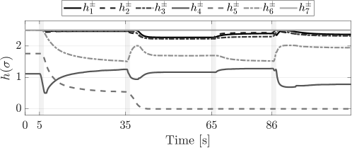
(a)

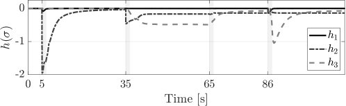
(b)

Figure 11: Values of the CBFs encoding the ESB tasks performed in the experiment with the KUKA LBR iiwa 7 R800. The time evolution of the joint limits avoidance functions $h^{\pm}_{i}$ for $i=1,...,7$ for both the upper and lower $i-$th joint limit are plotted in Fig. 11a. Figure 11b shows the evolution of ESB task functions $h_{i}$ for $i=1,2,3$, where a lower index value corresponds to a higher priority of the task. The tasks are: end-effector control to the $i$-th position $T_{p_{i}}$, position control of the third link $z$ coordinate $T_{z_{3}}$, and look-at-point vision task $T_{v}$. The time-varying stack of ESB tasks is: empty in the interval $[0,5)$, $T_{p_{1}}\prec T_{v}$ in $[5,\,35]$s, $T_{p_{1}}\prec T_{z_{3}}\prec T_{v}$ in $[35,\,65]$s, $T_{p_{1}}\prec T_{p_{2}}\prec T_{v}$ in $[65,\,86]$s, and $T_{p_{2}}\prec T_{p_{1}}\prec T_{v}$ after time $86$s. Light gray shaded areas denote transition intervals.

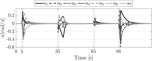
(a)

(b)

Figure 12: Joint velocity control input $u$, desired and measured joint positions recorded over the course of the experiment with the KUKA LBR iiwa 7 R800. Figure 12a shows the time evolution of the joint velocity control input highlighting switching time instants and transitions phases (shaded in light gray). Figure 12b plots desired and measured joint positions.

(a)

(b)

Figure 13: Time evolution of the QP slack variables during the experiment with the KUKA LBR iiwa 7 R800. Figure 13a shows the evolution of $\delta_{i}$ for $i=1,2,3$ that respectively relax the constraint of the task with $i-$th priority. Fig. 13b shows he components of the slack variable $v_{ij}$ for $i,j=1,2,3$ of the prioritization constraint. Light gray shaded areas denote transition intervals.

Figures 11, 12, and 13 show data recorded during the experiment. In Fig. 11a, the CBFs $h^{\pm}_{i}$ for $i=1,\dots,7$, of the joint limits avoidance task are depicted. As can be seen, they remain non-negative and ensure that each joint limit is not exceeded even if its limit value is reached, as happens to the fifth joint around $t=40$s ($h^{\pm}_{5}$ becomes zero). Figure 11b shows the task functions $h(\sigma)$. Notice that the functions $h(\sigma)$, encoding the ESB tasks, should be driven to zero. However, as can be seen in Fig. 11b, this does not happen whenever a physical limit is reached or when the prioritized stack is infeasible. In particular, in the interval $[5,35]\,$s, the stack is composed by two independent tasks, $T_{p_{1}}$ and $T_{v}$, and the functions $h_{1}$ and $h_{2}$ are driven to zero achieving faster convergence on the highest priority task (see Fig. 11). At time $t=35\,$s, the independent task $T_{z_{3}}$ is added but the task functions do not reach zero due to the hit of the fifth joint limit. The precedence relation $T_{p_{1}}\prec T_{z_{3}}\prec T_{v}$ is respected at steady state ($|h_{1}(\sigma)|<|h_{2}(\sigma)|<|h_{3}(\sigma)|$) even if the prioritization constraints are relaxed.

At time $t=65$s, task $T_{z_{3}}$ is replaced by $T_{p_{2}}$. Tasks $T_{p_{1}}$ and $T_{p_{2}}$ are dependent and only the one with the highest priority will be executed. The prioritization constraint corresponds to a greater relaxation of the lowest priority task and allows for a better execution of the highest highest priority task, whose corresponding CBF always achieves a value close to zero. Moreover, the relaxation of the constraint $T_{p_{2}}\prec T_{v}$ enables the decrease of the vision task function. Finally, at time $t=86$s, $T_{p_{1}}$ and $T_{p_{2}}$ are swapped, with analogous considerations. Computed joint velocities $u$ are plotted in Fig. 12a highlighting the continuity of the control input during stack switch and insertion/removal operations. Figure 12b shows the desired and measured joint positions and serves to illustrate how a good accuracy is achieved with the robot kinematic model using the control inputs in Fig. 12a and employing the control law (92). Finally, in Figures 13a and 13b the time evolution of the slack variables of the task execution constraints and the prioritization stack constraint are plotted, respectively. Together with the time evolution of the CBF values encoding the executed tasks reported in Fig. 11, these figures show how the constraint-based task execution and prioritization framework presented in this paper effectively achieves the desired robot behavior.

Further experiments were performed switching the described task stack manually in arbitrary sequences, with different end-effector desired positions and moving the Aruco tag to look at. Plots are here omitted for the sake of brevity but are shown in the accompanying video.

7 Conclusions

In this paper we introduced the concept of extended set-based (ESB) tasks used to encode the execution of robotic tasks via the forward invariance and asymptotic stability properties of appropriately defined sets of the robot state space. The concepts of orthogonality, independence, and dependence defined for Jacobian-based robotic tasks are shown to naturally extend to ESB tasks, carrying a similar meaning in terms of the possibility of concurrently executing multiple tasks. The control framework developed in the paper allows for an effective way of executing multiple ESB tasks and for a flexible way of prioritizing them in time-varying stacks. Theoretical results demonstrated stability properties of the prioritized task execution framework, giving guarantees on the expected robot behavior. Moreover, extensive simulations showcased several features and use cases suitable for the proposed approach. Furthermore, experiments performed on a real manipulator demonstrated how the developed control strategy is suitable to be employed in the tight loop under real time constraints.

References

- [AAC09] Gianluca Antonelli, Filippo Arrichiello, and Stefano Chiaverini. Experiments of formation control with multirobot systems using the null-space-based behavioral control. IEEE Transactions on Control Systems Technology, 17(5):1173–1182, 2009.
- [ACE+19] Aaron D. Ames, Samuel Coogan, Magnus Egerstedt, Gennaro Notomista, Koushil Sreenath, and Paulo Tabuada. Control barrier functions: Theory and applications. In 2019 18th European control conference (ECC), pages 3420–3431. IEEE, 2019.
- [Ant09] Gianluca Antonelli. Stability analysis for prioritized closed-loop inverse kinematic algorithms for redundant robotic systems. IEEE Transactions on Robotics, 25(5):985–994, 2009.
- [ANWE20] Aaron D. Ames, Gennaro Notomista, Yorai Wardi, and Magnus Egerstedt. Integral control barrier functions for dynamically defined control laws. IEEE Control Systems Letters, 5(3):887–892, 2020.
- [BB98] Paolo Baerlocher and Ronan Boulic. Task-priority formulations for the kinematic control of highly redundant articulated structures. In Proceedings. 1998 IEEE/RSJ International Conference on Intelligent Robots and Systems. Innovations in Theory, Practice and Applications (Cat. No. 98CH36190), volume 1, pages 323–329. IEEE, 1998.
- [BB04] Paolo Baerlocher and Ronan Boulic. An inverse kinematics architecture enforcing an arbitrary number of strict priority levels. The visual computer, 20(6):402–417, 2004.
- [BP20] Erlend A. Basso and Kristin Y. Pettersen. Task-priority control of redundant robotic systems using control lyapunov and control barrier function based quadratic programs. IFAC-PapersOnLine, 53(2):9037–9044, 2020. 21th IFAC World Congress.
- [BV04] Stephen Boyd and Lieven Vandenberghe. Convex optimization. Cambridge university press, 2004.
- [Chi97] Stefano Chiaverini. Singularity-robust task-priority redundancy resolution for real-time kinematic control of robot manipulators. IEEE Transactions on Robotics and Automation, 13(3):398–410, 1997.
- [DLAAC18] Paolo Di Lillo, Filippo Arrichiello, Gianluca Antonelli, and Stefano Chiaverini. Safety-related tasks within the set-based task-priority inverse kinematics framework. In 2018 IEEE/RSJ International Conference on Intelligent Robots and Systems, pages 6130–6135, 2018.
- [ELW00] Heather A. Edwards, Yuandan Lin, and Yuan Wang. On input-to-state stability for time varying nonlinear systems. In Proceedings of the 39th IEEE Conference on Decision and Control (Cat. No. 00CH37187), volume 4, pages 3501–3506. IEEE, 2000.
- [EMW14] Adrien Escande, Nicolas Mansard, and Pierre-Brice Wieber. Hierarchical quadratic programming: Fast online humanoid-robot motion generation. The International Journal of Robotics Research, 33(7):1006–1028, 2014.
- [FBP20] Marco Faroni, Manuel Beschi, and Nicola Pedrocchi. Inverse kinematics of redundant manipulators with dynamic bounds on joint movements. IEEE Robotics and Automation Letters, 5(4):6435–6442, 2020.
- [FDK15] Fabrizio Flacco, Alessandro De Luca, and Oussama Khatib. Control of Redundant Robots under Hard Joint Constraints: Saturation in the Null Space. IEEE Transactions on Robotics, 31(3):637–654, 2015.
- [Kha15] Hassan K Khalil. Nonlinear control. Pearson New York, 2015.
- [KWMK11] François Keith, Pierre Brice Wieber, Nicolas Mansard, and Abderrahmane Kheddar. Analysis of the discontinuities in prioritized tasks-space control under discrete task scheduling operations. IEEE International Conference on Intelligent Robots and Systems, pages 3887–3892, 2011.
- [LKCK22] Donghyeon Lee, Dongwoo Ko, Wan Kyun Chung, and Keehoon Kim. Quadratic programming-based task scaling for safe and passive robot arm teleoperation. IEEE/ASME Transactions on Mechatronics, 2022.
- [LTP16] Mingxing Liu, Yang Tan, and Vincent Padois. Generalized hierarchical control. Autonomous Robots, 40(1):17–31, Jan 2016.
- [MAT+16] Signe Moe, Gianluca Antonelli, Andrew R Teel, Kristin Y Pettersen, and Johannes Schrimpf. Set-based tasks within the singularity-robust multiple task-priority inverse kinematics framework: General formulation, stability analysis, and experimental results. Frontiers in Robotics and AI, 3:16, 2016.
- [MCR96] Éric Marchand, François Chaumette, and Alessandro Rizzo. Using the task function approach to avoid robot joint limits and kinematic singularities in visual servoing. In Proceedings of IEEE/RSJ International Conference on Intelligent Robots and Systems. IROS’96, volume 3, pages 1083–1090. IEEE, 1996.
- [MR99] A.R. Meenakshi and C. Rajian. On a product of positive semidefinite matrices. Linear algebra and its applications, 295(1-3):3–6, 1999.
- [MR13] Dejan Milutinovic and Jacob Rosen. Redundancy in robot manipulators and multi-robot systems. Springer, 2013.
- [MRC09] Nicolas Mansard, Anthony Remazeilles, and François Chaumette. Continuity of varying-feature-set control laws. IEEE Transactions on Automatic Control, 54(11):2493–2505, 2009.
- [MTAP15] Signe Moe, Andrew R Teel, Gianluca Antonelli, and Kristin Y Pettersen. Stability analysis for set-based control within the singularity-robust multiple task-priority inverse kinematics framework. In 2015 54th IEEE conference on decision and control (CDC), pages 171–178. IEEE, 2015.
- [Nag42] Mitio Nagumo. Über die lage der integralkurven gewöhnlicher differentialgleichungen. Proceedings of the Physico-Mathematical Society of Japan. 3rd Series, 24:551–559, 1942.
- [NE19] Gennaro Notomista and Magnus Egerstedt. Constraint-driven coordinated control of multi-robot systems. In 2019 American control conference (ACC), pages 1990–1996. IEEE, 2019.
- [NE21] Gennaro Notomista and Magnus Egerstedt. Persistification of robotic tasks. IEEE Transactions on Control Systems Technology, 29(2):756–767, 2021.
- [NHY87] Yoshihiko Nakamura, Hideo Hanafusa, and Tsuneo Yoshikawa. Task-priority based redundancy control of robot manipulators. The International Journal of Robotics Research, 6(2):3–15, 1987.
- [NME+21] Gennaro Notomista, Siddharth Mayya, Yousef Emam, Christopher Kroninger, Addison Bohannon, Seth Hutchinson, and Magnus Egerstedt. A resilient and energy-aware task allocation framework for heterogeneous multirobot systems. IEEE Transactions on Robotics, 38(1):159–179, 2021.
- [NMHE19] Gennaro Notomista, Siddharth Mayya, Seth Hutchinson, and Magnus Egerstedt. An optimal task allocation strategy for heterogeneous multi-robot systems. In 2019 18th European Control Conference (ECC), pages 2071–2076. IEEE, 2019.
- [NMS+20] Gennaro Notomista, Siddharth Mayya, Mario Selvaggio, María Santos, and Cristian Secchi. A set-theoretic approach to multi-task execution and prioritization. In 2020 IEEE International Conference on Robotics and Automation (ICRA), pages 9873–9879. IEEE, 2020.
- [NS16] Quan Nguyen and Koushil Sreenath. Exponential control barrier functions for enforcing high relative-degree safety-critical constraints. In 2016 American Control Conference (ACC), pages 322–328, 2016.
- [SBG+20] Bartolomeo Stellato, Goran Banjac, Paul Goulart, Alberto Bemporad, and Stephen Boyd. Osqp: An operator splitting solver for quadratic programs. Mathematical Programming Computation, 12(4):637–672, 2020.
- [SC16] Enrico Simetti and Giuseppe Casalino. A novel practical technique to integrate inequality control objectives and task transitions in priority based control. Journal of Intelligent & Robotic Systems, 84(1):877–902, 2016.
- [SCRC19] João Silvério, Sylvain Calinon, Leonel Rozo, and Darwin G. Caldwell. Learning task priorities from demonstrations. IEEE Transactions on Robotics, 35(1):78–94, 2019.
- [SHV+06] Mark W Spong, Seth Hutchinson, Mathukumalli Vidyasagar, et al. Robot modeling and control, volume 3. Wiley New York, 2006.
- [Son08] Eduardo D Sontag. Input to state stability: Basic concepts and results. In Nonlinear and optimal control theory, pages 163–220. Springer, 2008.
- [SS91] Jean-Jacques Slotine and Bruno Siciliano. A general framework for managing multiple tasks in highly redundant robotic systems. In Proceeding of 5th International Conference on Advanced Robotics, volume 2, pages 1211–1216, 1991.
- [SSB10] Günter Schreiber, Andreas Stemmer, and Rainer Bischoff. The fast research interface for the kuka lightweight robot. In 2010 International Conference on Robotics and Automation, page 7, 05 2010.
- [SSVO10] Bruno Siciliano, Lorenzo Sciavicco, Luigi Villani, and Giuseppe Oriolo. Robotics: modelling, planning and control. Springer Science & Business Media, 2010.