Efficient deep data assimilation with sparse observations and time-varying sensors

Abstract

Variational Data Assimilation (DA) has been broadly used in engineering problems for field reconstruction and prediction by performing a weighted combination of multiple sources of noisy data. In recent years, the integration of deep learning (DL) techniques in DA has shown promise in improving the efficiency and accuracy in high-dimensional dynamical systems. Nevertheless, existing deep DA approaches face difficulties in dealing with unstructured observation data, especially when the placement and number of sensors are dynamic over time. We introduce a novel variational DA scheme, named Voronoi-tessellation Inverse operator for VariatIonal Data assimilation (VIVID), that incorporates a DL inverse operator into the assimilation objective function. By leveraging the capabilities of the Voronoi-tessellation and convolutional neural networks, VIVID is adept at handling sparse, unstructured, and time-varying sensor data. Furthermore, the incorporation of the DL inverse operator establishes a direct link between observation and state space, leading to a reduction in the number of minimization steps required for DA. Additionally, VIVID can be seamlessly integrated with Proper Orthogonal Decomposition (POD) to develop an end-to-end reduced-order DA scheme, which can further expedite field reconstruction. Numerical experiments in a fluid dynamics system demonstrate that VIVID can significantly outperform existing DA and DL algorithms. The robustness of VIVID is also accessed through the application of various levels of prior error, the utilization of varying numbers of sensors, and the misspecification of error covariance in DA.

Main Notations

$\textbf{X}_{t}$	state field in the full space at time $t$
$N_{x},M_{x}$	dimension of the state space
$\textbf{x}_{t}$	flattened state field
$\hat{\textbf{x}}_{t}$	compressed state vector in the reduced space
$\textbf{Y}_{t}$	full observation field at time $t$
$N_{y},M_{y}$	dimension of the observation space
$(i_{t,k},j_{t,k})_{k=1...k^{*}}$	sensor positions in observation space
$\{y_{t,k}\}_{k=1...k^{*}}$	observed values at $(i_{t,k},j_{t,k})_{k=1...k^{*}}$
$R_{t,k}$	the Voronoi cell associated to $y_{t,k}$
$\tilde{\textbf{Y}}_{t}$	tessellated observation field based on $y_{t,k}$ and $R_{t,k}$
$\textbf{y}_{t}$	flattened observation vector
${\textbf{x}}_{b,t},\hat{\textbf{x}}_{b,t}$	background state in full and reduced space at time $t$
${\textbf{x}}_{v,t},\hat{\textbf{x}}_{v,t}$	machine-learned state in full and reduced space at time $t$
${\textbf{x}}_{a,t},\hat{\textbf{x}}_{a,t}$	analysis state in full and reduced space at time $t$
$\mathcal{H}_{t},\hat{\mathcal{H}}_{t}$	transformation operator in full and reduced spaces
$\mathcal{X}$	ensemble of state field snapshots
${\textbf{L}}_{\mathcal{X},q}$	POD projection operator with truncation parameter $q$
${\textbf{B}}_{t},\hat{\textbf{B}}_{t}$	background error covariance matrices in full and reduced spaces
${\textbf{R}}_{t},\hat{\textbf{R}}_{t}$	observation error covariance matrices in full and reduced spaces
${\textbf{P}}_{t},\hat{\textbf{P}}_{t}$	error covariance matrices of the inverse operator in full and reduced spaces
$\mathcal{J}_{t}$	objective function of variational data assimilation
$L$	correlation scale length in prior error covariances
$L^{E}$	estimated correlation scale length in prior error covariances

1 Introduction

The application of variational Data Assimilation (DA) is widespread in engineering problems, serving the purpose of state estimation and/or parameter identification. Variational DA is performed through a weighted combination of multiple sources of noisy data [1]. The goal of variational DA is to estimate the initial conditions of a system such that its subsequent evolution matches with real-world observations. The DA technique involves solving an optimization problem to find the best initial conditions or states and then integrating the system equations of motion over time to make predictions. DA has been widely applied in ocean engineering [2, 1], Numerical Weather Prediction (NWP) [3], nuclear engineering [4] and hydrology [5, 6]. However, traditional DA algorithms are encumbered by the computational demands arising from the numerous iterations necessary to solve the intricate optimization problem, particularly in cases where the observation data is unstructured and the placement of sensors is dynamic over time [7, 8].

In recent years, the use of machine learning in conjunction with DA has shown promise in further improving the efficiency and accuracy of predictions in high-dimensional dynamical systems [9, 10, 11, 12, 13, 14, 15]. Among these approaches, many of them aim to surrogate directly some key elements in DA such as the forward operator [15, 11, 14, 16], the transformation function [17], the reduced-order modelling (ROM) [12, 18] and the optimization process [19] using Machine Learning (ML) techniques. Recent research [20, 21] also aims to build end-to-end Deep Learning (DL) frameworks to emulate the entire DA procedure. In essence, the use of physics-based models in DA is being replaced, to some extent, by data-driven operators. Although machine learning models are powerful and efficient, physical models still provide benefits such as generalizability, interpretability, and consistency in established physical principles [22]. Additionally, physical models offer the advantage of coupling processes of different spatial and temporal scales, which is vital for complex forecasting applications [23]. Compared to pure data-driven DA methods, a more promising path might be to enhance physics-driven DA schemes with ML.

Given these circumstances, significant efforts have been directed towards enhancing the efficiency of physics-driven DA through the utilization of ML techniques [24, 25, 26], rather than solely relying on ML to replace traditional DA methods. In particular, the recent work of [27] introduces the learned observation operator in the variational assimilation scheme, enhancing and facilitating the optimization of the DA objective function. More precisely, a DL model is built to map the observation space to the state space. The assimilation scheme proposed by [27] then consists of a two-stage minimization procedure with the machine-learned inverse operator and the full transformation function, respectively. The former acts as an initialization step of the latter, which is a conventional variational assimilation algorithm. In other words, [27] doesn’t modify the objective function in DA and the ML inverse operator is only used to provide an advanced initialization point in the subsequent optimization. In addition, based on a traditional Convolutional Neural Network (CNN) structure, their method can only handle structured observations (e.g., square grids) with a fixed number of sensors (if not retrained) which limits its application in real-world problems where incomplete/sparse observations and time-varying sensors are prevalent [28, 29].

Geometric deep learning methods, namely Graph Neural Network (GNN), have been used to deal with unstructured data [30, 31]. However, it is widely noticed that training high-dimensional GNN can be computationally expensive and time-consuming [32, 33]. The recent work of [34] makes use of Voronoi tessellation [35] to address the bottleneck of sparse observations and various numbers of sensors in CNN-based field reconstruction. More precisely, a Voronoi tessellation is used to partition the input data into distinct regions based on the proximity of placed sensors. The resulting tessellation can be used to generate a set of Voronoi cells, where each cell represents a distinct region of the input space. This tessellation is then used as input to train a CNN model to reconstruct the whole underlying physical field. Such method, known as Voronoi-tessellation Convolutional Neural Network (VCNN), demonstrates strong performance in both synthetic Computational Fluid Dynamics (CFD) data and real geophysical fields [34], compared to traditional field interpolation approaches such as Kriging [36]. However, it is worth mentioning that mapping the sparse observation space to the whole physical field is often ill-defined. As a consequence, the prediction can be biased by the training dataset. Integrating a prior estimation, as performed in DA, can constrain the full physical space, thus addressing the issue of an ill-defined system. To the best of the author’s knowledge, none DA or Bayesian approaches with VCNN has been proposed in the existing literature.

In this paper, we introduce a novel DL-assisted DA approach, named Voronoi-tessellation Inverse operator for VariatIonal Data assimilation (VIVID), that couples a VCNN-based inverse operator in the DA. Unlike [27], VIVID is an end-to-end DA scheme that minimizes jointly the background mismatch in the state space, the inverse mismatch in the state space and the observation mismatch in the observation space. Similar to DA, the weight of different components in the objective function is determined by the estimated error covariance matrices. In fact, conventional DA can provide accurate local correction where the observations are dense, while VCNN is capable of delivering a global field prediction based on the knowledge extracted from historical data. By definition, the proposed VIVID incorporates the strength of both methods. In addition, by including a prior state-observation mapping provided by VCNN, the optimization of the DA objective function can be speeded-up, resulting in potentially fewer minimization iterations. To reduce the computational burden of DA for high-dimensional systems, much effort is given to performing DA in reduced order spaces [11, 37, 15]. In this paper, we incorporate a projection-based ROM, namely Proper Orthogonal Decomposition (POD), with the novel VIVID approach. In VIVID-ROM, instead of performing POD on top of the inverse operator, we build an end-to-end neural network that directly maps the tessellated observation space to the reduced state space with a similar structure as a vision encoder [38]. VIVID-ROM, as a variant of VIVID, clearly brings more insight into applying the developed approach in mainstream DA frameworks where ROM is often required.

As mentioned in [27], in many applications (e.g., NWP, geophysics), ample training data from historical observations can be found to train VCNN and VIVID. As a proof of concept, we perform extensive numerical experiments in this study on a shallow water CFD model [39]. The proposed VIVID is compared against the conventional variational DA and VCNN in terms of both reconstruction accuracy and computational efficiency. The reconstruction is evaluated using Relative Root Mean Square Error (R-RMSE) and Structural Similarity Index Measure (SSIM) where the former computes the pixel-wise reconstruction error and the latter measures the global similarity between reconstructed fields and the ground truth. In addition, we extensively assess the robustness of different approaches regarding background error, observation error, varying number of sensors and error covariance misspecification. The last one significantly impacts assimilation performance, raising broad research interests in the past two decades [40, 41].

In summary, we make the following main contributions in this study,

• We introduce a novel DL-assisted DA approach VIVID and its reduced order variant VIVID-ROM, which is capable of assimilating data from sparse, position-varying and number-varying sensors that current Deep DA approaches (e.g., [18, 11, 14, 17]) can not handle.

• Numerical experiments on a two-dimensional CFD test case show that the proposed VIVID substantially outperforms the variational DA and the state-of-the-art DL field reconstruction method VCNN by reducing the R-RMSE of around 50%. VIVID also requires around $70\%$ less computational time compared to conventional DA.

• The robustness of the proposed approach, regarding different noise levels and DA assumptions, is extensively studied in this paper. Within all numerical experiments implemented, VIVID achieves an outstanding performance in comparison with variational DA and VCNN.

The rest of this paper is organized as follows. Section 2 reminds the formulation of variational DA and the minimization loops of its objective function. Section 3 introduces the methodology of VIVID and its reduced order variant VIVID-ROM. Numerical experiments on a shallow water model with various conditions and assumptions are presented in Section 4. We close the paper with a discussion in Section 5.

2 Background: Variational data assimilation

The goal of DA is to enhance the identification/reconstruction of some physical fields $\textbf{X}_{t}\in\mathbb{R}^{\{N_{x},M_{x}\}}$ at a given time step $t$. Let us denote $\textbf{x}_{t}$, the flatten vector associated to $\textbf{X}_{t}$, i.e., $\textbf{x}_{t}\in\mathbb{R}^{\{N_{x}\times M_{x},1\}}$. DA makes use of two types of information: a prior forecast of the current state vector $\textbf{x}_{t}$, also known as the background state $\textbf{x}_{b,t}$, and an observation vector represented by $\textbf{y}_{t}$. The theoretical value of the state variable at time $t$ is denoted by $\textbf{x}_{\textrm{true},t}$, also known as the true state. Variational DA seeks the optimal balance between $\textbf{x}_{b,t}$ and $\textbf{y}_{t}$ by minimizing the cost function $J$ that is defined as:

$$J_{t}(\textbf{x}) =\frac{1}{2}(\textbf{x}-\textbf{x}_{b,t})^{T}\textbf{B}_{t}^{-1}(\textbf{x}-\textbf{x}_{b,t})+\frac{1}{2}(\textbf{y}_{t}-\mathcal{H}_{t}(\textbf{x}))^{T}\textbf{R}_{t}^{-1}(\textbf{y}_{t}-\mathcal{H}_{t}(\textbf{x}_{t}))$$ (1)

$$=\frac{1}{2}||\textbf{x}-\textbf{x}_{b,t}||^{2}_{\textbf{B}_{t}^{-1}}+\frac{1}{2}||\textbf{y}_{t}-\mathcal{H}_{t}(\textbf{x})||^{2}_{\textbf{R}_{t}^{-1}}$$

where $\mathcal{H}_{t}$ is the state-observation mapping function that links the flattened state vector to the flattened observation vector. $(\cdot)^{T}$ in Equation  (1) is the transpose operator. $\textbf{B}_{t}$ and $\textbf{R}_{t}$ denote the error covariance matrices in relation to $\textbf{x}_{b,t}$ and $\textbf{y}_{t}$, that is,

$$\textbf{B}_{t}=\textrm{Cov}(\epsilon_{b,t},\epsilon_{b,t}),\quad\textbf{R}_{t}=\textrm{Cov}(\epsilon_{y,t},\epsilon_{y,t}),$$ (2)

where

$$\epsilon_{b,t}=\textbf{x}_{b,t}-\textbf{x}_{\textrm{true},t},\quad\epsilon_{y,t}=\mathcal{H}_{t}(\textbf{x}_{\textrm{true},t})-\textbf{y}_{t}.$$ (3)

Prior errors $\epsilon_{b},\epsilon_{y}$ are often assumed to be centred Gaussian thus they can be fully characterised by $\textbf{B}_{t}$ and $\textbf{R}_{t}$,

$$\epsilon_{b,t}\sim\mathcal{N}(0,\textbf{B}_{t}),\quad\epsilon_{y,t}\sim\mathcal{N}(0,\textbf{R}_{t}).$$ (4)

Equation (1) is known as the three-dimensional variational (3D-Var) formulation, yielding a general objective function of variational DA. The point of minimum in Equation (1) is the analysis state $\textbf{x}_{a,t}$,

$$\textbf{x}_{a,t}=\underset{\textbf{x}}{\operatornamewithlimits{argmin}}\Big{(}J_{t}(\textbf{x})\Big{)}.$$ (5)

In the case where $\mathcal{H}_{t}$ can be approximated by a linear function $\textbf{H}_{t}$, the optimization of Equation (1) can be solved by Best Linear Unbiased Estimator (BLUE) [1],

$$\textbf{x}_{a,t}=\textbf{x}_{b,t}+\textbf{K}_{t}(\textbf{y}_{t}-\textbf{H}_{t}\textbf{x}_{b,t}),$$ (6)

where the Kalman gain matrix $\textbf{K}_{t}$ is defined as

$$\textbf{K}_{t}=\textbf{B}_{t}\textbf{H}_{t}^{T}(\textbf{H}_{t}\textbf{B}_{t}\textbf{H}_{t}^{T}+\textbf{R}_{t})^{-1}.$$ (7)

Following Equation (6), we can also obtain an output error covariance estimation $\textbf{A}_{t}$,

$$\textbf{A}_{t}=(\textbf{I}-\textbf{K}_{t}\textbf{B}_{t}\textbf{H}_{t})\textbf{B}_{t}.$$ (8)

The trace of the analysis covariance matrix, i.e., $Tr(\textbf{A}_{t})$, representing the total variance of posterior error, is often used as an indicator to evaluate the assimilation accuracy [1, 42].

When $\mathcal{H}_{t}$ is non-linear, approximate iterative methods [43] have been widely used to solve variational data assimilation. To do so, one has to compute the gradient $\nabla J(\textbf{x})$, which can be approximated by

$$\nabla J(\textbf{x})\approx 2\textbf{B}_{t}^{-1}(\textbf{x}-\textbf{x}_{b,t})-2\textbf{H}^{T}\textbf{R}_{t}^{-1}(\textbf{y}_{t}-\mathcal{H}_{t}(\textbf{x})).$$ (9)

In equation (9), H is obtained via a local linearization in the neighborhood of the current vector x. The minimization of 3D-Var is often performed via quasi-Newton methods, including for instance, BFGS approaches [44], where each iteration can be written as:

$$\textbf{x}_{k+1}=\textbf{x}_{k}-L_{\textrm{3D-Var}}\big{[}\textrm{Hess}(J)(\textbf{x}_{k})\big{]}^{-1}\nabla J(\textbf{x}_{k})$$ (10)

Here $k$ is the current iteration, and $L_{\textrm{3D-Var}}>0$ is the learning rate of the descent algorithm, and

$$\textrm{Hess}\Big{(}J(\textbf{x}=[x_{0},...,x_{n-1}])\Big{)}_{i,j}=\frac{\partial^{2}J}{\partial x_{i}\partial x_{j}}$$ (11)

is the Hessian matrix related to the cost function $J$. The process of the iterative minimization algorithm is summarised in Algorithm 1, where the approximation of the Hessian matrix is derived from the analytical formulation by solving only first-order sensitivities [45].

Algorithm 1 Iterative minization of 3D-Var cost function via quasi-Newton methods

1:Inputs: $\textbf{x}_{b,t},\textbf{y}_{t},\textbf{B}_{t},\textbf{R}_{t},\mathcal{H}_{t}$

2:parameters: $k_{\textrm{max}}$ , $\epsilon$

3:$\textbf{x}_{0}=\textbf{x}_{b},$ $k=0$

4:

5:while $k<k_{\textrm{max}}$ and $||\nabla J_{t}(\textbf{x}_{k})||>\epsilon$  do

6:     $J_{t}(\textbf{x}_{k})=\frac{1}{2}||\textbf{x}_{k}-\textbf{x}_{b,t}||^{2}_{\textbf{B}_{t}^{-1}}+\frac{1}{2}||\textbf{y}_{t}-\mathcal{H}_{t}(\textbf{x}_{k})||^{2}_{\textbf{R}_{t}^{-1}}$

7:     linearize $\textbf{H}_{t}\approx\mathcal{H}_{t}$ in the neighbourhood of $\textbf{x}_{k}$

8:     $\nabla J_{t}(\textbf{x}_{k})\approx 2\textbf{B}_{t}^{-1}(\textbf{x}_{k}-\textbf{x}_{b,t})-2\textbf{H}^{T}\textbf{R}_{t}^{-1}(\textbf{y}_{t}-\mathcal{H}_{t}(\textbf{x}_{k}))$

9:     compute the approximated Hessian matrix $\textrm{Hess}\big{(}J_{t}(\textbf{x}_{k})\big{)}$

10:     $\textbf{x}_{k+1}=\textbf{x}_{k}-L_{\textrm{3D-Var}}\big{[}\textrm{Hess}(J)\textbf{x}_{k}\big{]}^{-1}\nabla J_{t}(\textbf{x}_{k})$

11:     k = k+1

12:end while

output: $\textbf{x}_{k}$

3 Methodology

In this section, we describe the methodology of the proposed deep data assimilation scheme VIVID, including a machine learning inverse operator for unstructured observations and the DL-assisted variational DA formulation.

3.1 Voronoi tessellation for inverse operator

In this study, with a similar idea as [34], we build an inverse operator to map sparse and unstructured observations to the state space. We consider an observation field $\textbf{Y}_{t}\in\mathbb{R}^{N_{y}\times M_{y}}$ as a set of observable points (sensors) at a given time $t$, located at $\{(i_{t,k},j_{t,k})\}$ where

$$\{i_{t,k},j_{t,k}\}\in[1,...,N_{y}]\times[1,...,M_{y}]\quad\textrm{and}\quad\textrm{$k*$ is the number of sensors}.$$ (12)

$\{y_{t,k}\}_{k=1...k^{*}}$ are the observed values. A Voronoi cell $R_{t,k}$ associated to the observation $\{y_{t,k},i_{t,k},j_{t,k}\}$ can be defined as

$$R_{t,k}=\big{\{}\{i_{y},j_{y}\}\hskip 5.69054pt|\hskip 5.69054ptd((i_{y},j_{y}),(i_{t,k},j_{t,k}))\leq d((i_{y},j_{y}),(i_{t,q},j_{t,q})),\hskip 5.69054pt\forall\hskip 5.69054pt1\leq q\leq k^{*}\hskip 5.69054pt\textrm{and}\hskip 5.69054ptq\neq k\big{\}}.$$ (13)

Here, $d(\cdot)$ is the Euclidean distance, i.e.,

$$d((i_{y},j_{y}),(i_{t,k},j_{t,k}))=\sqrt{(i_{y}-i_{t,k})^{2}+(j_{y}-j_{t,k})^{2}},$$ (14)

where $\{i_{y},j_{y}\}\in[1,...,N_{y}]\times[1,...,M_{y}]$. Therefore, the observation space can be split into several Voronoi cells regardless of the number of sensors, that is,

$$\{(i_{y},j_{y})\}=\bigcup_{k=1}^{k*}R_{t,k}\quad\textrm{and}\quad R_{t,k}\cap R_{t,q}=\emptyset\quad(\forall\quad k\neq q).$$ (15)

A tessellated observation $\tilde{\textbf{Y}}_{t}=\{\tilde{y}_{t,i_{y},j_{y}}\}\in\mathbb{R}^{N_{y}\times M_{y}}$ in the full observation space can be obtained by

$$\tilde{y}_{t,i_{y},j_{y}}=y_{t,k}\quad\textrm{if}\quad(i_{y},j_{y})\in R_{t,k}.$$ (16)

The tessellation $\tilde{\textbf{Y}}_{t}$ is then used as input for training a deep learning model to map the unobservable state field $\textbf{X}_{t}$. To do so, a CNN is employed, i.e.,

$$\tilde{\textbf{Y}}_{t}\xrightarrow{\hskip 17.07182pt\text{CNN}\hskip 17.07182pt}\textbf{X}_{t}.$$ (17)

The CNN implemented in this study consists of 7 convolution layers with ReLu activation function [46] and 48 channels [34]. The large number of channels ensure the representation capacity of the Neural Network (NN) and, more importantly, improve the robustness to variations regarding different sensor placement. A cropping or upsampling layer is also added to reshape the two-dimensional field from $(N_{y},M_{y})$ to $(N_{x},M_{x})$, if different. The workflow of Voronoi tessellation-assisted observation-state mapping is illustrated in Figure 1 and the exact CNN structure is shown in Table 1.

Table 1: NN structure of the CNN with $\tilde{\textbf{Y}}_{t}$ as input and ${\textbf{X}}_{t}$ as output

Layer (type)	Output Shape	Activation
Input	$(N_{y},M_{y},1)$
Conv 2D $(8\times 8)$	$(N_{y},M_{y},48)$	ReLu
Conv 2D $(8\times 8)$	$(N_{y},M_{y},48)$	ReLu
Conv 2D $(8\times 8)$	$(N_{y},M_{y},48)$	ReLu
Conv 2D $(8\times 8)$	$(N_{y},M_{y},48)$	ReLu
Conv 2D $(8\times 8)$	$(N_{y},M_{y},48)$	ReLu
Conv 2D $(8\times 8)$	$(N_{y},M_{y},48)$	ReLu
Cropping 2D	$(N_{x},M_{x},48)$
Conv 2D	$(N_{x},M_{x},1)$	ReLu

It is worth mentioning that despite the dimension of $\tilde{\textbf{Y}}_{t}$ equals to $\{N_{y},M_{y}\}$, by construction, its degree of freedom remains as the number of sensors $k$. As a consequence, Equation (17) represents an under-determined system when $k<N_{x}\times M_{y}$. This is most likely since the observations in DA are often assumed sparse and incomplete [1]. Therefore, performing field reconstruction using solely VCNN without DA can lead to ill-defined problems.

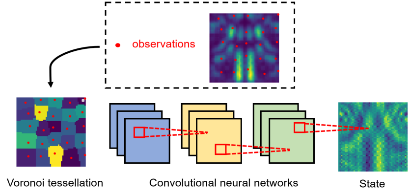
Figure 1: Flowchart of the Voronoi tessellation-assisted CNN to map the state field using sparse observations

3.2 Voronoi-tessellation Inverse operator for VariatIonal Data assimilation (VIVID)

In the proposed DA approach of this paper, the machine-learned observation-state operator plays a pivotal role in enhancing the DA accuracy and accelerating the minimization convergence. Denoting $\textbf{x}_{v,t}=\textrm{CNN}(\tilde{\textbf{Y}}_{t})$ as the flattened output of the CNN (Table 1) applied on $\tilde{\textbf{Y}}_{t}$, the objective function of the proposed variational DA reads

$$J_{t}(\textbf{x}) =\frac{1}{2}||\textbf{x}-\textbf{x}_{b,t}||^{2}_{\textbf{B}_{t}^{-1}}+\frac{1}{2}||\textbf{x}-\textbf{x}_{v,t}||^{2}_{\textbf{P}_{t}^{-1}}+\frac{1}{2}||\textbf{y}_{t}-\mathcal{H}_{t}(\textbf{x})||^{2}_{\textbf{R}_{t}^{-1}},$$ (18)

where $\textbf{P}_{t}$ denotes the error covariance matrix of the learned operator. The minimization of Equation (18) follows the same process as the traditional variational DA. The proposed DA algorithm scheme can be summarized in Figure 2 and algorithm 2.

Algorithm 2 Formulation and minization of the proposed variational DA

1:Inputs: $\textbf{x}_{b,t},\textbf{y}_{t},\textbf{B}_{t},\textbf{R}_{t},\textbf{P}_{t},\mathcal{H}_{t}$

2:parameters: $k_{\textrm{max}}$ , $\epsilon$

3:$\textbf{x}_{0}=\textbf{x}_{b},$ $k=0$

4:$\tilde{\textbf{Y}}_{t}\xleftarrow{\hskip 17.07182pt\text{Voronoi}\hskip 17.07182pt}\textbf{y}_{t}$

5:compute $\textbf{x}_{v,t}=\textrm{CNN}(\tilde{\textbf{Y}}_{t})$

6:

7:while $k<k_{\textrm{max}}$ and $||\nabla J_{t}(\textbf{x}_{k})||>\epsilon$  do

8:     $J_{t}(\textbf{x}_{k})=\frac{1}{2}||\textbf{x}_{k}-\textbf{x}_{b,t}||^{2}_{\textbf{B}_{t}^{-1}}+\frac{1}{2}||\textbf{x}_{k}-\textbf{x}_{v,t}||^{2}_{\textbf{P}_{t}^{-1}}+\frac{1}{2}||\textbf{y}_{t}-\mathcal{H}_{t}(\textbf{x}_{k})||^{2}_{\textbf{R}_{t}^{-1}}$

9:     linearize $\textbf{H}_{t}\approx\mathcal{H}_{t}$ in the neighbourhood of $\textbf{x}_{k}$

10:     $\nabla J_{t}(\textbf{x}_{k})\approx 2\textbf{B}_{t}^{-1}(\textbf{x}_{k}-\textbf{x}_{b,t})+2\textbf{P}_{t}^{-1}(\textbf{x}_{k}-\textbf{x}_{v,t})-2\textbf{H}_{t}^{T}\textbf{R}_{t}^{-1}(\textbf{y}_{t}-\mathcal{H}_{t}(\textbf{x}_{k}))$

11:     compute the approximated Hessian matrix $\textrm{Hess}\big{(}J_{t}(\textbf{x}_{k})\big{)}$

12:     $\textbf{x}_{k+1}=\textbf{x}_{k}-L_{\textrm{3D-Var}}\big{[}\textrm{Hess}(J)\textbf{x}_{k}\big{]}^{-1}\nabla J_{t}(\textbf{x}_{k})$

13:     k = k+1

14:end while

output: $\textbf{x}_{k}$

As for the specification of $\textbf{P}_{t}$, it can be empirically estimated using an independent validation dataset which is different from the training dataset, that is,

$${\textbf{P}}_{t}\approx\frac{1}{n_{\text{val}}-1}\sum_{\text{val dataset}}({\textbf{x}}_{t}-\textbf{x}_{v,t})\left({\textbf{x}}_{t}-\textbf{x}_{v,t}\right)^{T}.$$ (19)

To regularize the estimated ${\textbf{P}}_{t}$ matrix, covariance localization is implemented in this study, thanks to the Gaspari-Cohn localization function [47] defined as:

$$G(\rho)=\begin{cases}\text{if 0 $\leq$ $\rho$ $<$ 1: }&1-\frac{5}{3}\rho^{2}+\frac{5}{8}\rho^{3}+\frac{1}{2}\rho^{4}-\frac{1}{4}\rho^{5}\\ \text{if 1 $\leq$ $\rho$ $<$ 2: }&4-5\rho+\frac{5}{3}\rho^{2}+\frac{5}{8}\rho^{3}-\frac{1}{2}\rho^{4}+\frac{1}{12}\rho^{5}-\frac{2}{3\rho}\\ \ \text{if $\rho$ $\geq$ 2: }&0\end{cases}\quad\textrm{with}\quad\rho=\frac{r}{L}.$$ (20)

Here, $r$ denotes the spatial distance of two points in the state space and $L$ is an empirically defined correlation scale length. The localized covariance matrix can then be obtained,

$$\forall{{P}}_{t}^{a,b}\in{\textbf{P}}_{t},\quad{P}_{t}^{a,b}\longleftarrow{P}_{t}^{a,b}\cdot G(\rho),\quad\text{with}\quad\omega=\frac{d(a,b)}{L},\quad\{a,b\}\in[1,...,N_{x}\times M_{x}],$$ (21)

where $\omega(\cdot)$ denotes a distance metric in the state space. Here we remind that ${\textbf{P}}_{t}\in\mathbb{R}^{(N_{x}\times M_{x})^{2}}$ is the error covariance matrix of flattened state vectors. Thus, the locations $a,b$ are with two-dimensional indices in the state space.

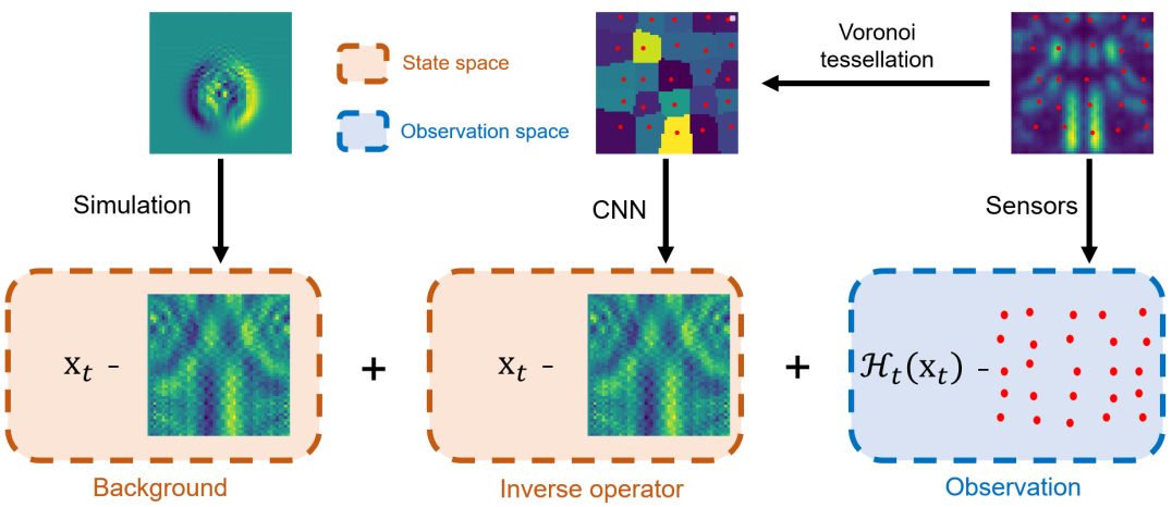
Figure 2: Flowchart of the proposed deep DA approach

3.3 Posterior error analysis for a linear case

Considering a new observation vector $\bar{\textbf{y}}_{t}$ as the concatenation of ${\textbf{x}}_{v,t}$ and $\textbf{y}_{t}$. Equation (18) can be re-written as:

$$J_{t}(\textbf{x})=\frac{1}{2}||\textbf{x}-\textbf{x}_{b,t}||^{2}_{\textbf{B}_{t}^{-1}}+\frac{1}{2}||\bar{\textbf{y}}_{t}-\bar{\mathcal{H}}_{t}(\textbf{x})||^{2}_{\bar{\textbf{R}}_{t}^{-1}},$$ (22)

where

$$\bar{\textbf{y}}_{t}=\begin{pmatrix}\textbf{x}_{v,t}\\ {\textbf{y}}_{t}\end{pmatrix},\quad\bar{\textbf{H}}_{t}=\begin{pmatrix}\textbf{I}\\ {\textbf{H}}_{t}\end{pmatrix},\quad\bar{\textbf{R}}_{t}=\begin{pmatrix}\textbf{P}_{t}&0\\ 0&{\textbf{R}}_{t}\end{pmatrix}.$$ (23)

Similar to Equations (8) and (6), when $\mathcal{H}_{t}$ can be approximated by a linear operator $\mathcal{H}_{t}\approx\textbf{H}_{t}$, the minimization of Equation (22) can be performed through the BLUE formulation,

$$\textbf{x}_{a,t} =\textbf{x}_{b,t}+\bar{\textbf{K}}_{t}(\bar{\textbf{y}}_{t}-\bar{\textbf{H}}_{t}\textbf{x}_{b,t}),$$ (24)

$$\textbf{A}_{t} =(\textbf{I}-\bar{\textbf{K}}_{t}\bar{\textbf{H}}_{t})\textbf{B}_{t}.$$ (25)

with the modified Kalman gain matrix,

$$\bar{\textbf{K}}_{t}=\textbf{B}_{t}\bar{\textbf{H}}_{t}^{T}(\bar{\textbf{H}}_{t}\textbf{B}_{t}\bar{\textbf{H}}_{t}^{T}+\bar{\textbf{R}}_{t})^{-1}=\big{(}\textbf{B}_{t},\textbf{B}_{t}\textbf{H}_{t}\big{)}\cdot\begin{pmatrix}\textbf{B}_{t}+\textbf{P}_{t}&\textbf{B}_{t}\textbf{H}_{t}^{T}\\ \textbf{H}_{t}\textbf{B}_{t}&\textbf{H}\textbf{B}_{t}\textbf{H}_{t}^{T}+\textbf{R}_{t}\end{pmatrix}^{-1}.$$ (26)

For the simplicity of illustration, we show the evolution of $Tr(\textbf{A}_{t})$ in function of $\textbf{B}_{t}$, $\textbf{P}_{t}$ and $\textbf{R}_{t}$ in a simple scalar case as being done in [42]. In the particular case of a one-dimensional problem, $\{\textbf{A}_{t}(=Tr(\textbf{A}_{t})),\textbf{B}_{t},\textbf{R}_{t},\textbf{P}_{t},\textbf{H}_{t}\}\in\mathbb{R}^{5}$. Therefore Equation (8) and (25) can be simplified to:

$$\textbf{A}^{\textrm{DA}}_{t} =\frac{\textbf{B}_{t}\textbf{R}_{t}}{\textbf{B}_{t}\textbf{H}^{2}_{t}+\textbf{R}_{t}},$$ (27)

$$\textbf{A}^{\textrm{VIVID}}_{t} =\textbf{B}_{t}\Bigg{(}\frac{\textbf{B}_{t}^{2}\textbf{H}^{2}_{t}}{\textbf{B}_{t}\textbf{H}^{2}_{t}\textbf{P}_{t}+\textbf{B}_{t}\textbf{R}_{t}+\textbf{P}_{t}\textbf{R}_{t}}-\frac{\textbf{B}_{t}\left(\textbf{B}_{t}\textbf{H}^{2}_{t}+\textbf{R}_{t}\right)}{\textbf{B}_{t}\textbf{H}^{2}_{t}\textbf{P}_{t}+\textbf{B}_{t}\textbf{R}_{t}+\textbf{P}_{t}\textbf{R}_{t}}$$

$$-\textbf{H}_{t}\left(-\frac{\textbf{B}_{t}^{2}\textbf{H}_{t}}{\textbf{B}_{t}\textbf{H}^{2}_{t}\textbf{P}_{t}+\textbf{B}_{t}\textbf{R}_{t}+\textbf{P}_{t}\textbf{R}_{t}}+\frac{\textbf{B}_{t}\textbf{H}_{t}(\textbf{B}_{t}+\textbf{P}_{t})}{\textbf{B}_{t}\textbf{H}^{2}_{t}\textbf{P}_{t}+\textbf{B}_{t}\textbf{R}_{t}+\textbf{P}_{t}\textbf{R}_{t}}\right)+1\Bigg{)}.$$ (28)

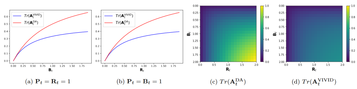
Figure 3: The evolution of $Tr(\mathbf{A}^{\textrm{DA}}_{t})$ and $Tr(\mathbf{A}^{\textrm{VIVID}}_{t})$ regarding $\textbf{B}_{t}$ and $\textbf{R}_{t}$

We are interested in the sensitivity of $Tr(\textbf{A}^{\textrm{DA}}_{t})$ and $Tr(\textbf{A}^{\textrm{VIVID}}_{t})$ with respect to $\textbf{B}_{t}$, $\textbf{R}_{t}$ and $\textbf{P}_{t}$. Without loss of generality, we suppose $\textbf{H}_{t}=\textbf{P}_{t}=1$ in the following illustrations while varying the values of $\textbf{B}_{t}$ and $\textbf{R}_{t}$. Figure 3 (a) (resp. (b)) illustrates the evolution of $Tr(\mathbf{A}^{\textrm{DA}}_{t})$ and $Tr(\mathbf{A}^{\textrm{VIVID}}_{t})$ while varying $\textbf{B}_{t}$ (resp. $\textbf{R}_{t}$) from 0 to 2. Since the transformation matrix is set to be $\textbf{H}_{t}=1$, as expected, symmetric curves can be found in Figure 3 (a) and (b). The posterior error variance can be significantly reduced thanks to VIVID, indicating a more accurate assimilation. Figure 3 (c) (resp. (d)) illustrates the value of $Tr(\mathbf{A}^{\textrm{DA}}_{t})$ (resp. $Tr(\mathbf{A}^{\textrm{VIVID}}_{t})$) while varying simultaneously $\textbf{B}_{t}$ and $\textbf{R}_{t}$. Consistent with Figure 3 (a) and (b), we find that the posterior error variance can be substantially reduced, especially when $\textbf{B}_{t}$ and $\textbf{R}_{t}$ are large. The results of this simple scalar problem demonstrate the strength when introducing another prior estimation, independent of the background state. A detailed numerical comparison of the proposed VIVID approach against conventional DA and VCNN, is performed with a CFD experiment in Section 4.

3.4 VIVID with reduced order modelling

Performing DA in the full physical space, even with the help of the machine learning inverse operator, can be computationally expensive and time consuming due to the large dimension of the state space. Here, we explain how the proposed approach can be coupled with a ROM using POD to further improve its efficiency.

Considering a set of $n_{\textrm{state}}$ state snapshots, from one or several simulations/predictions, are represented by a matrix $\mathcal{X}\in\mathbb{R}^{(\{N_{x}\times M_{x})\times n_{\textrm{state}}\}}$ where each column of $\mathcal{X}$ represents a flattened state at a given time step, that is,

$$\mathcal{X}=\big{[}\textbf{x}_{0}\big{|}\textbf{x}_{1}\big{|}...\big{|}\textbf{x}_{n_{\textrm{state}}-1}\big{]}.$$ (29)

The empirical covariance $\textbf{C}_{\mathcal{X}}$ of $\mathcal{X}$ can be computed and decomposed as

$$\textbf{C}_{\mathcal{X}}=\frac{1}{n_{\textrm{state}}-1}\mathcal{X}\mathcal{X}^{T}={\textbf{L}}_{\mathcal{X}}{\textbf{D}}_{\mathcal{X}}{{\textbf{L}}_{\mathcal{X}}}^{T}$$ (30)

where the columns of ${\textbf{L}}_{\mathcal{X}}$ represent the principal components of $\mathcal{X}$ and ${\textbf{D}}_{\mathcal{X}}$ is a diagonal matrix with the corresponding eigenvalues $\{\lambda_{\mathcal{X},i},i=0,...,n_{\textrm{state}}-1\}$ in a decreasing order,

$${\textbf{D}}_{\mathcal{X}}=\begin{bmatrix}\lambda_{\mathcal{X},0}&&\\ &\ddots&\\ &&\lambda_{\mathcal{X},n_{\textrm{state}}-1}\end{bmatrix}.$$ (31)

To compress the state variables to a reduced space of dimension $q\hskip 5.69054pt(q\in\mathbb{N}^{+}\hskip 5.69054pt\textrm{and}\hskip 5.69054ptq\leq n_{\textrm{state}})$, we compute a projection operator ${\textbf{L}}_{\mathcal{X},q}$ by keeping the first $q$ columns of ${\textbf{L}}_{\mathcal{X}}$. ${\textbf{L}}_{\mathcal{X}}$ can be obtained via performing Singular Value Decomposition (SVD) [48] which does not require the estimation of the full covariance matrix $\textbf{C}_{\mathcal{X}}$. For a flattened state field $\textbf{x}_{t}$, the reduced latent vector $\hat{\textbf{x}}_{t}$ reads

$$\hat{\textbf{x}}_{t}={{\textbf{L}}_{\mathcal{X},q}}^{T}\textbf{x}_{t},$$ (32)

which is an approximation to the full vector $\textbf{x}_{t}$.

The latent vector $\hat{\textbf{x}}_{t}$ can be decompressed to a full space vector $\textbf{x}_{t}^{r}$ by

$$\textbf{x}_{t}^{r}={{\textbf{L}}_{\mathcal{X},q}}\hat{\textbf{x}}_{t}={{\textbf{L}}_{\mathcal{X},q}}\textrm{Tr}({{\textbf{L}}_{\mathcal{X},q}})\textbf{x}_{t}.$$ (33)

The POD compression rate $\rho_{\textbf{x}}$ and the energy conservation rate $\gamma_{\textbf{x}}$ are defined as:

$$\gamma_{\textbf{x}}=\sum_{i=0}^{q-1}\lambda^{2}_{\mathcal{X},i}\Big{/}\sum_{i=0}^{n_{\textrm{state}}-1}\lambda^{2}_{\mathcal{X},i}\quad\textrm{and}\quad\rho_{\textbf{x}}=q\big{/}n_{\textrm{state}}.$$ (34)

To reduce the DA computational cost, the assimilation can be carried out in the space of $\hat{\textbf{x}}_{t}$ instead of $\textbf{x}_{t}$, leading to a new state-observation operator $\hat{\mathcal{H}}_{t}$, defined as

$$\hat{\mathcal{H}}_{t}=\mathcal{H}_{t}\circ{{\textbf{L}}_{\mathcal{X},q}}\quad\textrm{with}\quad\textbf{y}_{t}=\mathcal{H}_{t}(\textbf{x}_{t})=\mathcal{H}_{t}\circ{{\textbf{L}}_{\mathcal{X},q}}(\hat{\textbf{x}}_{t})=\hat{\mathcal{H}}_{t}(\hat{\textbf{x}}_{t}).$$ (35)

It is worth mentioning that the POD here is conducted on uncentered data. This choice is made to retain the original scale and distribution of the data, ensuring a meaningful low-dimensional representation and enabling the data learning mapping function to uncover the underlying physics. As for the ML inverse operator, instead of applying POD to the CNN output, we propose an end-to-end CNN, named $\text{CNN}_{\text{ROM}}$, from the tessellated observation to the compressed vector $\textbf{x}_{t}$, that is,

$$\tilde{\textbf{Y}}_{t}\xrightarrow{\hskip 17.07182pt\text{CNN}_{\text{ROM}}\hskip 17.07182pt}\hat{\textbf{x}}_{t}.$$ (36)

The $\text{CNN}_{\text{ROM}}$ follows the classical structure of convolutional encoder with Maxpooling layers [49] as shown in Table 2. Finally, the objective function of deep data assimilation with ROM can be written as

$$J_{t}(\hat{\textbf{x}}) =\frac{1}{2}||\hat{\textbf{x}}-\hat{\textbf{x}}_{b,t}||^{2}_{\hat{\textbf{B}}_{t}^{-1}}+\frac{1}{2}||\hat{\textbf{x}}-\hat{\textbf{x}}_{v,t}||^{2}_{\hat{\textbf{P}}_{t}^{-1}}+\frac{1}{2}||\textbf{y}_{t}-\hat{\mathcal{H}}_{t}(\hat{\textbf{x}})||^{2}_{\textbf{R}_{t}^{-1}},$$ (37)

where

$$\hat{\textbf{x}}_{v,t}=\text{CNN}_{\text{ROM}}(\tilde{\textbf{Y}}_{t})\quad\textrm{and}\quad\hat{\textbf{B}}_{t}={{\textbf{L}}_{\mathcal{X},q}}^{T}{\textbf{B}}_{t}{{\textbf{L}}_{\mathcal{X},q}}.$$ (38)

The minimization of Equation (37) can be performed through Algorithm 2 with $(\hat{\textbf{x}}_{b,t},\textbf{y}_{t},\hat{\textbf{B}}_{t},\hat{\textbf{R}}_{t},\hat{\textbf{P}}_{t},\hat{\mathcal{H}}_{t})$ as inputs instead of $(\textbf{x}_{b,t},\textbf{y}_{t},\textbf{B}_{t},\textbf{R}_{t},\textbf{P}_{t},\mathcal{H}_{t})$ .

Table 2: NN structure of the CNN with $\tilde{\textbf{Y}}_{t}$ as input and $\hat{\textbf{x}}_{t}$ as output

Layer (type)	Output Shape	Activation
Input	$(N_{y},M_{y},1)$
Conv 2D $(8\times 8)$	$(N_{y},M_{y},16)$	ReLu
Conv 2D $(8\times 8)$	$(N_{y},M_{y},16)$	ReLu
Maxpooling $(2\times 2)$	$(\lceil N_{y}/2\rceil,\lceil M_{y}/2\rceil,16)$
Conv 2D $(4\times 4)$	$(\lceil N_{y}/2\rceil,\lceil M_{y}/2\rceil,16)$	ReLu
Maxpooling $(2\times 2)$	$(\lceil N_{y}/4\rceil,\lceil M_{y}/4\rceil,16)$
Conv 2D $(4\times 4)$	$(\lceil N_{y}/4\rceil,\lceil M_{y}/4\rceil,16)$	ReLu
Flatten	$(\lceil N_{y}/4\rceil\times\lceil M_{y}/4\rceil\times 16)$
Dense(q)	$q$

4 Numerical experiments

In this section, we illustrate the numerical results in a two-dimensional CFD system. The proposed deep DA approach is compared against conventional DA and the VCNN approach. We show the robustness of VIVID against varying prior error levels, different sensor numbers and error covariance misspecifications. Two metrics, namely R-RMSE and SSIM are used to evaluate the difference and the similarity between the assimilated and the true state, respectively.

4.1 Description of the shallow water system and experiments set up

Here we consider a standard shallow-water fluid mechanics system which is broadly used for evaluating the performance of DA approaches (e.g., [50], [51], [6]). We consider a non-linear wave-propagation problem. The initial condition consists of a cylinder of water with a certain radius that is released at $\textit{t}=0$. Here, we assume that the horizontal length scale is more important than the vertical one. The Coriolis force is also neglected. These lead to the following Saint-Venant equations ([39]) coupling the horizontal fluid velocity and height:

$$\frac{\partial u}{\partial t} =-g\frac{\partial}{\partial x}(h)-bu$$ (39)

$$\frac{\partial v}{\partial t} =-g\frac{\partial}{\partial y}(h)-bv$$

$$\frac{\partial h}{\partial t} =-\frac{\partial}{\partial x}(uh)-\frac{\partial}{\partial y}(vh)$$

$$u_{t=0} =0$$

$$v_{t=0} =0$$

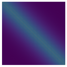
Figure 4: The error covariance matrix with scale correlation length $L=5$ for a flattened state vector

where $(u,v)$ denote the two dimensional fluid velocity (in $0.1m/s$) and $h$ represents the fluid height (in $mm$). The earth gravity constant $g$ is thus scaled to 1 and the dynamical system is set in a non-conservative form. The initial velocity fields are set to zero for both $u$ and $v$. The height of the water cylinder is set as $h_{p}$ $mm$ higher than the still water and the radius of the initial water cylinder is set to be $r_{w}$ $mm$. $h_{p}$ and $r_{w}$ are considered as hyperparameters in this modelling. The study area of $(50mm\times 50mm)$ is discretized with a squared grid of size $(N_{x}=50,M_{x}=50)$ and the solution of Eq. (39) is approximated using a first order finite difference method. The time integration is also performed using a finite difference scheme with a time interval $\delta t=10^{-6}s$.

In this study, we focus on the reconstruction of the velocity field $u$ based on sparse and time-varying sensors and noisy prior forecasts. For the latter, Gaussian spatial-correlated noises are added to the simulated $u$ field, more precisely, a Matérn covariance kernel function of order $3/2$ is employed,

$$\phi(r)=(1+\frac{r}{L})\exp(-\frac{r}{L}),$$ (40)

where $r,L$ are the spatial distance and the correlation scale length defined in Equation (20). In other words,

$$\textbf{x}_{t}=u_{t},\quad\textbf{x}_{b,t}=\textbf{x}_{t}+s_{b}\cdot\epsilon_{b,t}\quad\textrm{and}\quad\epsilon_{b,t}\sim\mathcal{N}(0,\textbf{B}(\phi(L,r)),$$ (41)

where $s_{b}$ is the background error standard deviation and $\textbf{B}(\phi(r))$ represents the error correlation matrix of the flattened velocity field $\textbf{x}_{b,t}$. The subscript ${(.)}_{b}$ refers to the background (prior) information. In this paper, $\textbf{B}(\phi(L,r))$ is fixed with $L=5$ as shown in Figure 4. To evaluate the performance of the proposed assimilation approach in complex non-linear systems, a synthetic observation function is created to build the observation space $\textbf{Y}_{t}$. Different sensors $\{y_{t,k}\}_{k=1...k^{*}}$ with a random placement are chosen at each time step $t$. The details of the non-linear transformation function and the sensor placement choice are available in the appendix of this paper. An example of the dynamical velocity field with the associated background field, the full observation field and the tessllated observations (with 100 sensors) are illustrated in Figure 5. In this example, we fix $h_{p}=0.1mm,r_{w}=4mm$ in the simulation and the background error standard deviation is set to be $0.005$ (in $0.1m/s$).

As for the VCNN inverse operator, the train data consists of four simulations and the tests of both VCNN and VIVID are performed with an unseen simulation, as shown in Table 3. Each simulation consists of 10000 snapshots from $0s$ to $10^{-2}s$. The test dataset is significantly different from the train dataset, resulting in an average R-RMSE of 82.5% and an average SSIM of 0.917 as shown in Figure 6 (a,b).

The VCNN operator is trained on the Google Colab server with an NVIDIA T4 GPU. For a fair comparison, all DA approaches are performed on the same labtop CPU of Intel(R) Core(TM) i7-10810U with 16 GB Memory. The minimization of the objective function in DA (Equation (1) and (18)) is carried out using the BFGS approach with a stopping criteria [52] of tolerance $10^{-6}$. The truncation parameter $q$ (i.e., the dimension of the reduced space) is chosen as $q=100$ where the singular values reach a point of stagnation as shown in Figure 6 (c).

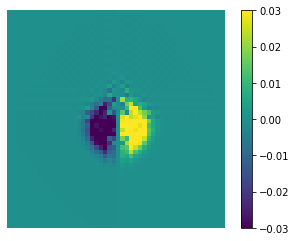
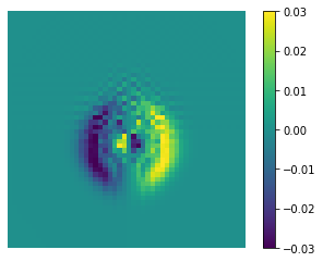
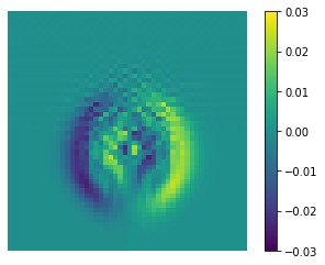
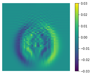
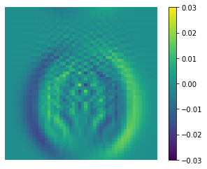
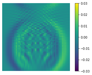
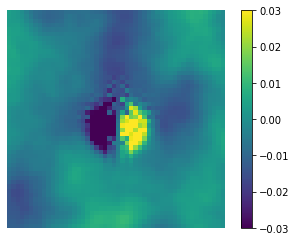
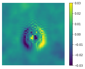
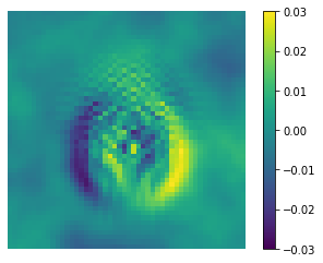
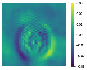
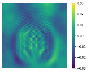
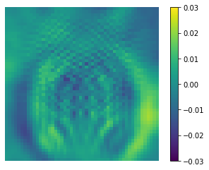
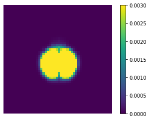
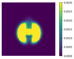
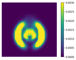
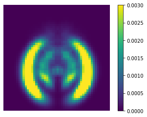
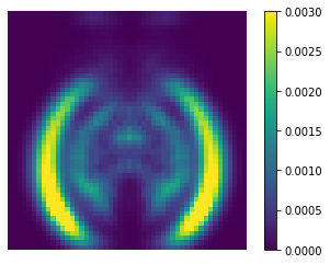
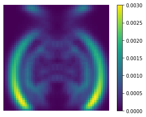
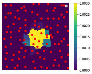
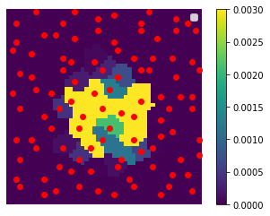
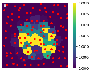
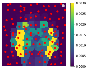
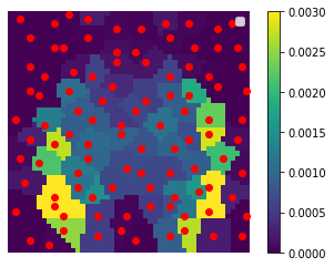
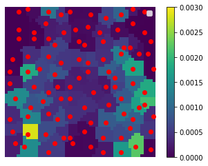
Figure 5: The evolution of the simulated velocity field (1st raw), the background velocity field (2nd raw), the complete observation space (3rd raw) and the tessllated observation field with 100 sensors (4th raw) at $\{5,10,15,20,25,30\}\times 10^{-4}s$ respectively.

Table 3: Model parameter choice in the train and test datasets

Parameter	Train				test
$h_{p}$	0.1	0.15	0.1	0.15	0.2
$r_{w}$	4	4	5	5	6

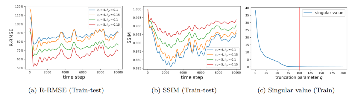
Figure 6: R-RMSE (a) and SSIM (b) between the train (4 different simulations) and the test data (1 simulation); Singular value of all the train data (c)

4.2 Numerical results and analysis of the shallow water experiments

In this section, we show extensive experiments to evaluate the performance of the proposed approach against conventional DA and only VCNN approaches, regarding both prediction accuracy and efficiency. In the test dataset, DA is performed on 20 snapshots (extracted every $5\times 10^{-4}s$) at different time steps. The simulation outputs are considered as ground truth, where spatially correlated errors are added to construct background states. In each DA, the sensor placement is randomly chosen with a given sensor number (see appendix).

4.2.1 Accuracy and efficiency

We first set the background error standard deviation to $0.02m/s$, leading to an R-RMSE of $0.62$ and a SSIM of 0.901 in average for all test samples. As shown in Figure 5, 100 time-varying sensors are placed randomly (with a given structure) in both train and test snapshots. The observations are first set to be error-free. Thus the observation error matrix is set to be $\textbf{R}_{t}=10^{-3}\cdot\textbf{I}$ to increase the confidence level of the observed data, where I denotes the identity matrix. The inverse operator covariance $\textbf{P}_{t}$ is empirically estimated and localized, as explained in Equation (19)-(21). The $\textbf{B}_{t}$ matrix with the Matern covariance kernel (Eqaution (40)) is supposed to be perfectly known here.

As illustrated in Table 4, all DA and DL methods can significantly reduce the R-RMSE and increase the SSIM. In particular, the proposed VIVID approach substantially outperforms conventional DA and VCNN in terms of assimilation accuracy. Furthermore, we find that VIVID can considerably reduce the computational time by decreasing the number of iterations required in the L-BFGS optimization for variational assimilation (see Algorithm 1 and 2). As observed in [53], the improvement of efficiency is due to the extra information provided by the DL inverse operator which links the observations directly to the state variables. In other words, the minimization loops can be better guided towards the observations in VIVID. The evolution of the DA objective functions against L-BFGS iterations is illustrated in Figure 8. It can be clearly noticed that the objective function of VIVID stabilizes much faster compared to the conventional DA both in the full and reduced space. It is worth mentioning that, unlike DL loss functions, the value of the objective function in DA does not necessarily represent the assimilation accuracy since the ground truth is not involved in DA objective functions.

Table 4:

Method	Accuracy		Efficiency
	R-RMSE	SSIM	iterations	time
background	0.62	0.901	-	-
DA	0.33	0.979	54.5	$\approx 42\text{min}$
VCNN	0.32	0.993	-	-
VIVID	0.14	0.998	15.1	$\approx 11\text{min}$
DA-ROM	0.49	0.984	19.1	$\approx 8s$
VCNN-ROM	0.33	0.992	-	-
VIVID-ROM	0.16	0.993	5.2	$\approx 2s$

Figure 9 illustrates the reconstructed velocity field at $t=0.04s$ and $t=0.08s$ with the mismatch against the ground truth (Figure 7). As shown by Figure 9 (f,n), the capability of DA is limited where the prior error is substantial and spatially correlated. On the other hand, VCNN manages to provide a good overall reconstruction (Figure 9 (c,k)), leading to a high SSIM in Table 4. However, the reconstruction noise is still significant (see Figure 9 (g,o)) due to the time-varying sensors and the difference between train and test datasets (see Table 3). In contrast, VIVID, by definition, combining the strength of conventional DA and VCNN, provides an accurate overall field reconstruction, which is consistent with the observation in Table 4. The same experiments, coupled with ROM, are shown in Figure 10. We find that the application of POD can not only reduce the computational cost (see Table 4) but also denoise the added background error. This is mainly because the constructed principle components have learned underlying physics information [54] despite the difference between train and test datasets. It is worth noting that the ROM has well understood the left-right symmetricity in the velocity field, resulting in symmetric reconstructed fields in DA, VCNN and VIVID. In comparison to the other two approaches, VIVID delivers the most accurate velocity field (Figure 10), leading to the best R-RMSE and SSIM score in Table 4.

In the previous experiments, VIVID shows outstanding performance both when being applied directly in the full physical space or coupled with a ROM. From now on, to facilitate direct comparison, we only apply different approaches in the full velocity field at $t=0.04s$ and evaluate their robustness against varying prior errors, sensor numbers and misspecified background error matrices.

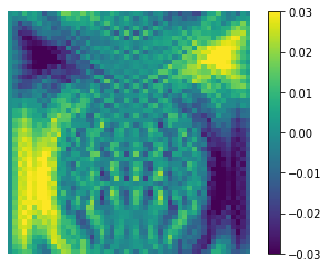
(a)

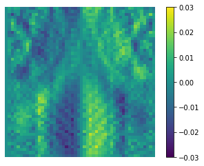
(b)

Figure 7: Simulated velocity field, considered as the ground truth in the numerical experiments

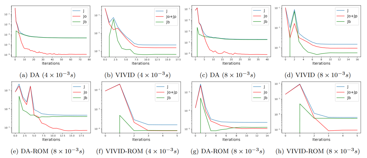
Figure 8: Minimization (L-BFGS) iterations in variational DA

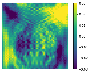
(a)

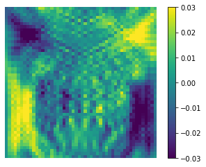
(b)

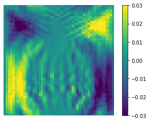
(c)

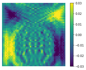
(d)

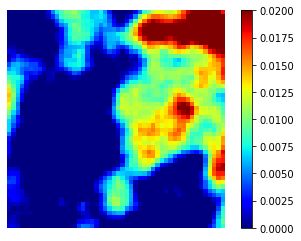
(e)

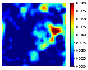
(f)

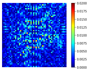
(g)

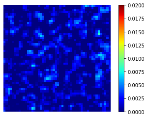
(h)

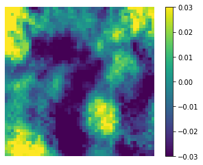
(i)

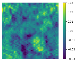
(j)

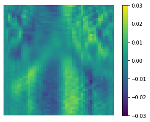
(k)

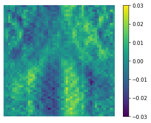
(l)

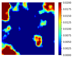
(m)

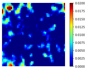
(n)

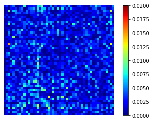
(o)

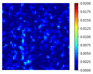
(p)

Figure 9: Background and assimilated velocity field at $t=0.04s$ (a-h) and $t=0.08s$ (i-p) compared to the ground truth

(a)

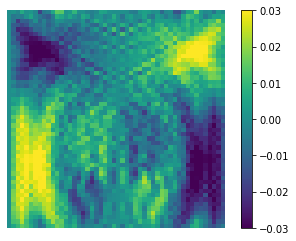
(b)

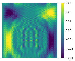
(c)

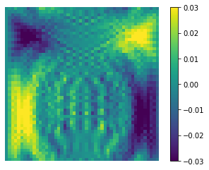
(d)

(e)

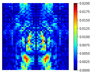
(f)

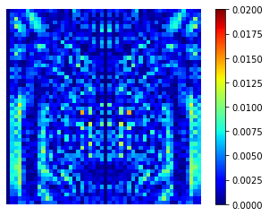
(g)

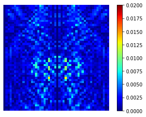
(h)

(i)

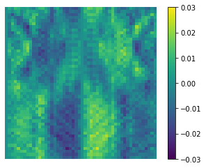
(j)

(k)

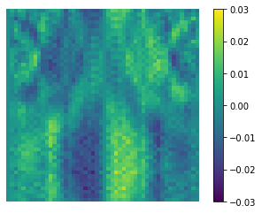
(l)

(m)

(n)

(o)

(p)

Figure 10: Background and assimilated (with ROM) velocity field at $t=0.04s$ (a-h) and $t=0.08s$ (i-p) compared to the ground truth

4.2.2 Varying background error

With the same spatial error correlation defined in Equation (40), we first vary the background error deviation from $(0.005,0.01,0.015,0.02,0.025,0.03)$ (in $m/s$). We plot the evolution of the reconstruction error in Figure 11 (a). As expected, the assimilation error of DA and VIVID increase against the background error standard deviation. However, VIVID is much less sensitive to the background error thanks to the VCNN inverse operator, which is not impacted by $\textbf{x}_{b}$. The experiments with a small background error deviation ($0.005m/s$) are illustrated in Figure 12. As observed, low background error (Figure 12 (f)) leads to accurate assimilation results (Figure 12 (g,h)). Despite that conventional DA outperforms VCNN when the background error is small, the proposed VIVID, combining the advantage of DA and DL, shows a significant advantage in reconstruction accuracy compared to the other two approaches.

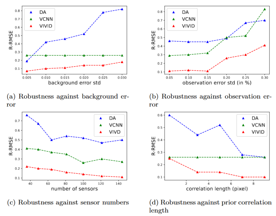
Figure 11: Evolution of R-RMSE according to different assimilation assumptions

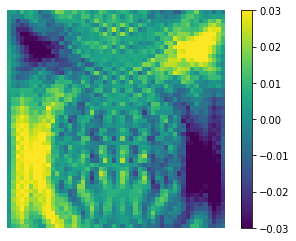
(a)

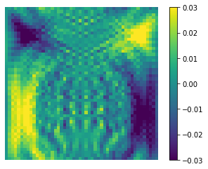
(b)

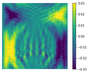
(c)

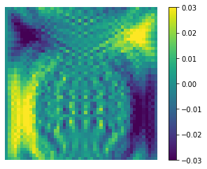
(d)

(e)

(f)

(g)

(h)

Figure 12: Background and assimilated velocity field at $t=0.04s$ with a background error of standard deviation of $0.005m/s$

4.2.3 Varying observation error

Until now, the observations are assumed error-free. To further explore the robustness of different approaches, spatial-independent observation errors are now added to the observation vector y. These observation errors are supposed to be relative, varying from $5\%$ to $30\%$, regarding the true observation value. As observed in Figure 11 (b), all methods are sensitive to the observation error, in particular VCNN which is trained with error-free observation data. Nonetheless, VIVID shows a consistent advantage in terms of R-RMSE regardless of the observation error. The assimilated fields with a relatively high observation error ($30\%$) is shown in Figure 13. Compared to error-free observations, suboptimal reconstruction results are observed in all three methods compared to Figure 9. Despite achieving the most accurate field reconstruction, VIVID is clearly impacted by the noise in both conventional DA and VCNN.

(a)

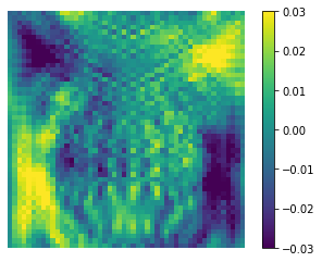
(b)

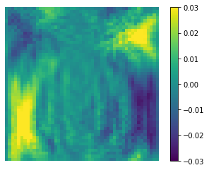
(c)

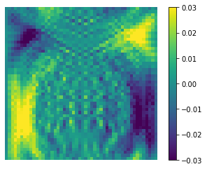
(d)

(e)

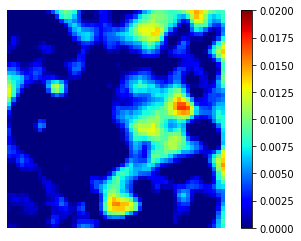
(f)

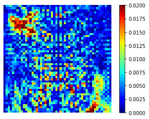
(g)

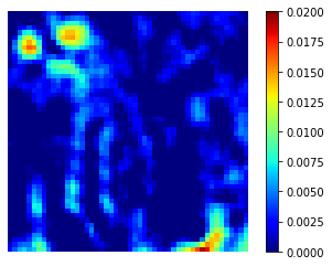
(h)

Figure 13: Background and assimilated velocity field at $t=0.04s$ with $30\%$ of observation error

4.2.4 Varying sensor numbers

We implement the experiments with various numbers of sensors. The sensors are randomly placed within a certain range $r_{s}=3$ (see appendix) to the standard placement (i.e., $6\times 6,7\times 7,...,12\times 12$ in this section). Clearly, a large number of sensors provide more observation information to the assimilation. On the other hand, VCNN is solely trained with $10\times 10=100$ sensors. To ensure the generalizability of the proposed approach, it is thus important to assess the robustness with different numbers of sensors. Figure 11 (c) illustrates the evolution of R-RMSE. It can be clearly observed that overall the R-RMSE decreases against the number of sensors, in particular, the R-RMSE of VIVID drops $50\%$ from 0.2 to 0.1. We illustrate the experiments with $36$ and $144$ sensors for comparison in Figure 14. Compared to Figure 9 (with 100 sensors), as expected, using only 36 sensors leads to suboptimal assimilation results due to the sparsity of observations. Furthermore, comparing Figure 14 (o) and Figure 9 (g), we can conclude that using 144 sensors also perturbs VCNN trained on data with 100 sensors. However, the different number of sensors only slightly impact the performance of VIVID as shown in Figure 14 (h,p).

(a)

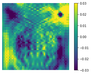
(b)

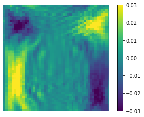
(c)

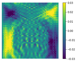
(d)

(e)

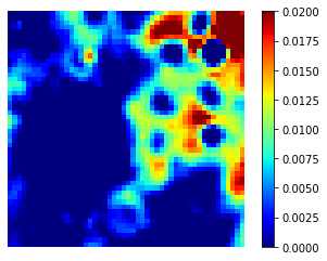
(f)

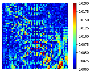
(g)

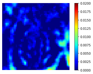
(h)

(i)

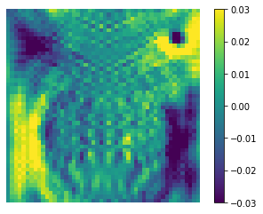
(j)

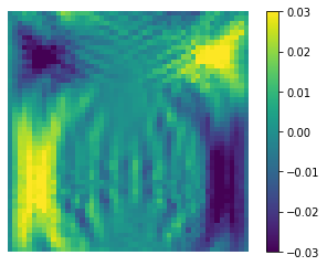
(k)

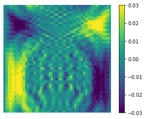
(l)

(m)

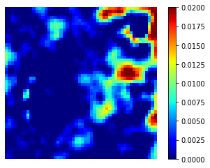
(n)

(o)

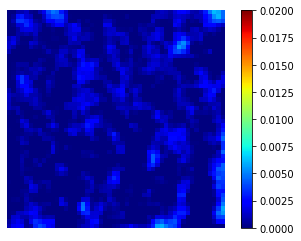
(p)

Figure 14: Background and assimilated velocity field at $t=0.04s$ with 36 (a-i) and 144 (a-i) sensors

4.2.5 misspecified covariance matrix

Misspecified error covariances can lead to suboptimal assimilation results [40]. Estimating these covariance matrices, especially the background matrix, has been a long-standing research challenge [40, 55, 41]. In this paper, we study the impact of misspecifying the background error correlation length $L$ defined in Equation (40). The background states in the numerical experiments are all generated with $L=5$ in this paper. Here, we vary the estimated correlation length $L^{E}$ with $L^{E}\in\{0.1,3,5,7,9\}$ (in pixel length). Notably, $L^{E}=0.1$ signifies that almost no spatial error correlation is considered in the assimilation procedure.

Figure 11 (d) depicts the influence of $L^{E}$ on assimilation R-RMSE knowing the exact correlation length is $L=5$. Underestimating the correlation length ($L^{E}<<L$) clearly leads to a high R-RMSE, indicating suboptimal assimilation for both conventional DA and VIVID. Surprisingly we find that overestimating the correlation length results in a more accurate field reconstruction for both DA and VIVID. The R-RMSE of VIVID stabilizes around 0.1 for $L^{E}>3$.

Figure 15 displays the assimilation outputs with $L^{E}=0.1$ and $L^{E}=9$. As shown in Figure 15 (a,e), the underestimation of the correlation length leads to insufficient use of the observation information, especially in conventional DA. Consistent with Figure 11, overestimation of the correlation length, in contrast, results in less assimilation error. In both cases, an advantage of VIVID is clearly identified. These results demonstrate the strength of VIVID when the background error is misspecified, which is applicable for a wide range of real-world DA problems.

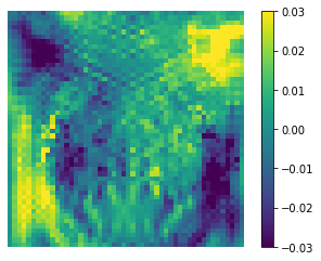
(a)

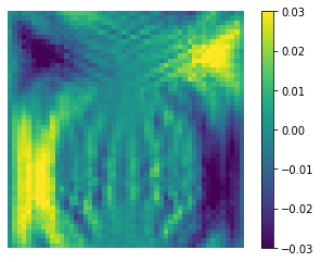
(b)

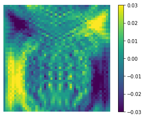
(c)

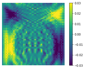
(d)

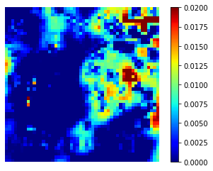
(e)

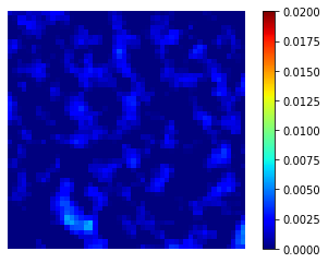
(f)

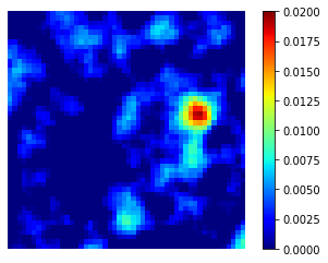
(g)

(h)

Figure 15: Background and assimilated velocity field at $t=0.04s$ with a background error of standard deviation of $0.005m/s$. The VCNN results are the same as in Figure 9

In summary, the results in this section with extensive numerical experiments show the consistent advantage of VIVID regarding the different levels of background error, observation error, number of sensors and misspecification of error covariances.

5 Discussion and future work

The majority of present-day deep DA techniques, particularly those relying on CNNs or Multi Layer Percepton (MLP), have limitations in their ability to handle observations that are sparse, unstructured, and with varying dimensions. This poses a significant challenge when attempting to apply these methods to industrial problems. In this paper, we proposed a novel variational DA scheme, named VIVID, which integrates a DL inverse operator in the assimilation objective function. By applying VCNN, VIVID is capable of dealing with sparse, unstructured, and time-varying sensors. In addition, the number of minimization steps in DA can be reduced thanks to the DL inverse operator that links directly the observations to the state space. We show in this paper that the proposed VIVID can also be coupled with POD to form an end-to-end reduced order DA scheme to further speed-up the field reconstruction. Thorough numerical evaluations performed in the present paper demonstrate the strength of VIVID in comparison against conventional DA and VCNN. As summarized in Figure 16, VIVID achieves high accuracy with a relatively low computational cost. It is worth noticing that by including prior estimations, VIVID forms a well-defined problem even with sparse observations, which is not the case for most DL-based reconstruction methods. Unlike conventional DA, VCNN, VIVID and other DL methods require offline data for training. Nevertheless, for various DA applications, such as NWP, hydrology or nuclear engineering, adequate historical data can be acquired from past observations.

The proposed approach can be naturally extended to include physical constraints [56] both in the DL projection or the assimilation objective function. Future works can also consider extending VIVID in a spatial-temporal DA scheme (e.g., Four-dimensional variational data assimilation (4Dvar)) where ConvLSTM [57] or Transformers [58] can be used to build the inverse operator for a sequence of observations. From a theoretical perspective, future work can also focus on quantifying the correlation between observation error and VCNN error in the DA formulation.

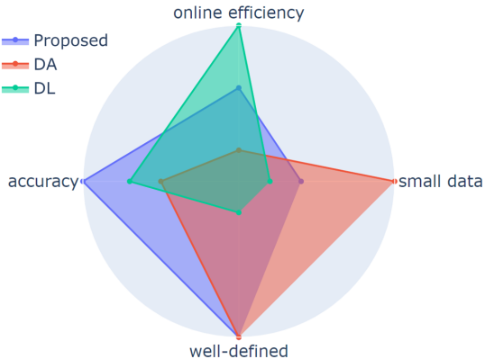
Figure 16: Comparison of the proposed approach against the state-of-the-art approaches

Appendix: Synthetic observations in the numerical experiments

Construction of the observation space

In the numerical experiments of the shallow water system, the state field $\textbf{X}_{t}$ consists of the horizontal velocity field $u$ in Equation (39). The synthetic full observation field $\textbf{Y}_{t}$ is set to be of the same dimension as $\textbf{X}_{t}$ (i.e., $N_{x}=N_{y}=M_{x}=M_{y}$ in this experiment). $\textbf{Y}_{t}$ is constructed as

$$\forall(i_{y},j_{y}) \in[1,...,M_{y}]\times[1,...,N_{y}],$$

$$Y_{t,i_{y},j_{y}} =0.5\sum_{(i_{x},j_{x})\in\rho_{1}(i_{y},j_{y})}X^{2}_{t,i_{x},j_{x}}+\sum_{(i_{x},j_{x})\in\rho_{2}(i_{y},j_{y})}\beta_{i_{x},j_{x}}X^{2}_{t,i_{x},j_{x}}.$$ (42)

Here,

$$\rho_{1}(i_{y},j_{y}) =\big{\{}\{i_{x},j_{x}\}\quad|\quad\sqrt{(i_{x}-i_{y})^{2}+(j_{x}-j_{y})^{2}}\leq 3\big{\}},$$ (43)

$$\rho_{2}(i_{y},j_{y}) =\big{\{}\{i_{x},j_{x}\}\quad|\quad\sqrt{(i_{x}-i_{y})^{2}+(j_{x}-j_{y})^{2}}\leq 1.5\big{\}},$$ (44)

representing two neighborhoods of different radius of the position $(i_{y},j_{y})$. In other words, the full synthetic observation field $\textbf{Y}_{t}$ represents a local weighted sum of state variable squares, as shown in Figure 17.

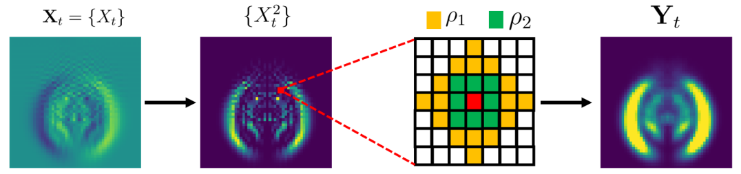
Figure 17: Computation of the non-linear observation field

Random sensor placement

Once $\textbf{Y}_{t}$ is computed, random sensor placement is performed based on structured grid points ($10\times 10$ in the training set and $6\times 6,7\times 7,...,12\times 12$ in the test set ) as shown in Figure 18. More precisely, a sensor is randomly positioned in the neighbourhood of each grid point within a sample range $r_{s}=3$. Thus the observations $\{y_{t,k}\}_{k=1...k^{*}}$ and the observation vector $\textbf{y}_{t}$ are differentiable with respect to the state $\textbf{X}_{t}$.

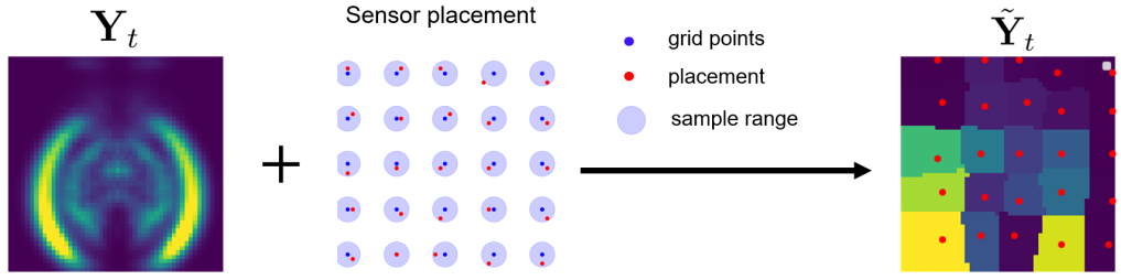
Figure 18: Random sensor placement according to structured grid points

Data and code availability

The code of the shallow water experiments is available at https://github.com/DL-WG/VIVID. Sample data and the script to generate experimental is also provided in the github reporsitory.

Acronyms

NN

Neural Network

ML

Machine Learning

LA

Latent Assimilation

DA

Data Assimilation

AE

Autoencoder

CAE

Convolutional Autoencoder

BLUE

Best Linear Unbiased Estimator

RNN

Recurrent Neural Network

CNN

Convolutional Neural Network

SSIM

Structural Similarity Index Measure

LSTM

long short-term memory

POD

Proper Orthogonal Decomposition

VIVID

Voronoi-tessellation Inverse operator for VariatIonal Data assimilation

VCNN

Voronoi-tessellation Convolutional Neural Network

SVD

Singular Value Decomposition

ROM

reduced-order modelling

CFD

Computational Fluid Dynamics

NWP

Numerical Weather Prediction

R-RMSE

Relative Root Mean Square Error

BFGS

Broyden–Fletcher–Goldfarb–Shanno

AI

artificial intelligence

DL

Deep Learning

KF

Kalman filter

MLP

Multi Layer Percepton

GNN

Graph Neural Network

GLA

Generalised Latent Assimilation

3Dvar

Three-dimensional variational data assimilation

4Dvar

Four-dimensional variational data assimilation

References

- Carrassi et al. [2018] A. Carrassi, M. Bocquet, L. Bertino, G. Evensen, Data assimilation in the geosciences: An overview of methods, issues, and perspectives, Wiley Interdisciplinary Reviews: Climate Change 9 (2018) e535.
- Elisseeff et al. [2002] P. Elisseeff, H. Schmidt, W. Xu, Ocean acoustic tomography as a data assimilation problem, IEEE Journal of Oceanic Engineering 27 (2002) 275–282.
- Lorenc et al. [2015] A. C. Lorenc, N. E. Bowler, A. M. Clayton, S. R. Pring, D. Fairbairn, Comparison of hybrid-4denvar and hybrid-4dvar data assimilation methods for global NWP, Monthly Weather Review 143 (2015) 212–229.
- Gong et al. [2022] H. Gong, S. Cheng, Z. Chen, Q. Li, Data-enabled physics-informed machine learning for reduced-order modeling digital twin: Application to nuclear reactor physics, Nuclear Science and Engineering (2022) 1–26.
- Liu et al. [2012] Y. Liu, A. Weerts, M. Clark, H.-J. Hendricks Franssen, S. Kumar, H. Moradkhani, D.-J. Seo, D. Schwanenberg, P. Smith, A. Van Dijk, et al., Advancing data assimilation in operational hydrologic forecasting: progresses, challenges, and emerging opportunities, Hydrology and earth system sciences 16 (2012) 3863–3887.
- Cheng et al. [2021] S. Cheng, J.-P. Argaud, B. Iooss, D. Lucor, A. Ponçot, Error covariance tuning in variational data assimilation: application to an operating hydrological model, Stochastic Environmental Research and Risk Assessment 35 (2021) 1019–1038.
- Apte et al. [2008] A. Apte, C. K. Jones, A. Stuart, J. Voss, Data assimilation: Mathematical and statistical perspectives, International journal for numerical methods in fluids 56 (2008) 1033–1046.
- Ghil and Malanotte-Rizzoli [1991] M. Ghil, P. Malanotte-Rizzoli, Data assimilation in meteorology and oceanography, in: Advances in geophysics, volume 33, Elsevier, 1991, pp. 141–266.
- Cheng et al. [2023] S. Cheng, C. Quilodrán-Casas, S. Ouala, A. Farchi, C. Liu, P. Tandeo, R. Fablet, D. Lucor, B. Iooss, J. Brajard, et al., Machine learning with data assimilation and uncertainty quantification for dynamical systems: a review, IEEE/CAA Journal of Automatica Sinica 10 (2023) 1361–1387.
- Farchi et al. [2021] A. Farchi, M. Bocquet, P. Laloyaux, M. Bonavita, Q. Malartic, A comparison of combined data assimilation and machine learning methods for offline and online model error correction, Journal of computational science 55 (2021) 101468.
- Cheng et al. [2022] S. Cheng, I. C. Prentice, Y. Huang, Y. Jin, Y.-K. Guo, R. Arcucci, Data-driven surrogate model with latent data assimilation: Application to wildfire forecasting, Journal of Computational Physics (2022) 111302.
- Cheng et al. [2023] S. Cheng, J. Chen, C. Anastasiou, P. Angeli, O. K. Matar, Y.-K. Guo, C. C. Pain, R. Arcucci, Generalised latent assimilation in heterogeneous reduced spaces with machine learning surrogate models, Journal of Scientific Computing 94 (2023) 11.
- Tang et al. [2020] M. Tang, Y. Liu, L. J. Durlofsky, A deep-learning-based surrogate model for data assimilation in dynamic subsurface flow problems, Journal of Computational Physics 413 (2020) 109456.
- Pawar et al. [2020] S. Pawar, S. E. Ahmed, O. San, A. Rasheed, I. M. Navon, Long short-term memory embedded nudging schemes for nonlinear data assimilation of geophysical flows, Physics of Fluids 32 (2020) 076606.
- Liu et al. [2022] C. Liu, R. Fu, D. Xiao, R. Stefanescu, P. Sharma, C. Zhu, S. Sun, C. Wang, Enkf data-driven reduced order assimilation system, Engineering Analysis with Boundary Elements 139 (2022) 46–55.
- Casas et al. [2020] C. Q. Casas, R. Arcucci, P. Wu, C. Pain, Y.-K. Guo, A reduced order deep data assimilation model, Physica D: Nonlinear Phenomena 412 (2020) 132615.
- Wang et al. [2022] Y. Wang, X. Shi, L. Lei, J. C.-H. Fung, Deep learning augmented data assimilation: Reconstructing missing information with convolutional autoencoders, Monthly Weather Review 150 (2022) 1977–1991.
- Peyron et al. [2021] M. Peyron, A. Fillion, S. Gürol, V. Marchais, S. Gratton, P. Boudier, G. Goret, Latent space data assimilation by using deep learning, Quarterly Journal of the Royal Meteorological Society 147 (2021) 3759–3777.
- Gottwald and Reich [2021] G. A. Gottwald, S. Reich, Supervised learning from noisy observations: Combining machine-learning techniques with data assimilation, Physica D: Nonlinear Phenomena 423 (2021) 132911.
- Fablet et al. [2022] R. Fablet, Q. Febvre, B. Chapron, Multimodal 4dvarnets for the reconstruction of sea surface dynamics from sst-ssh synergies, arXiv preprint arXiv:2207.01372 (2022).
- Filoche [2022] A. Filoche, Variational Data Assimilation with Deep Prior. Application to Geophysical Motion Estimation, Ph.D. thesis, Sorbonne université, 2022.
- Geer [2021] A. Geer, Learning earth system models from observations: machine learning or data assimilation?, Philosophical Transactions of the Royal Society A 379 (2021) 20200089.
- Stauffer and Seaman [1994] D. R. Stauffer, N. L. Seaman, Multiscale four-dimensional data assimilation, Journal of Applied Meteorology and Climatology 33 (1994) 416–434.
- Chattopadhyay et al. [2023] A. Chattopadhyay, E. Nabizadeh, E. Bach, P. Hassanzadeh, Deep learning-enhanced ensemble-based data assimilation for high-dimensional nonlinear dynamical systems, Journal of Computational Physics (2023) 111918.
- Ouala et al. [2018] S. Ouala, R. Fablet, C. Herzet, B. Chapron, A. Pascual, F. Collard, L. Gaultier, Neural network based kalman filters for the spatio-temporal interpolation of satellite-derived sea surface temperature, Remote Sensing 10 (2018) 1864.
- Buizza et al. [2022] C. Buizza, C. Q. Casas, P. Nadler, J. Mack, S. Marrone, Z. Titus, C. Le Cornec, E. Heylen, T. Dur, L. B. Ruiz, et al., Data learning: integrating data assimilation and machine learning, Journal of Computational Science 58 (2022) 101525.
- Frerix et al. [2021] T. Frerix, D. Kochkov, J. Smith, D. Cremers, M. Brenner, S. Hoyer, Variational data assimilation with a learned inverse observation operator, in: M. Meila, T. Zhang (Eds.), Proceedings of the 38th International Conference on Machine Learning, volume 139 of Proceedings of Machine Learning Research, PMLR, 2021, pp. 3449–3458.
- Barker et al. [2004] D. M. Barker, W. Huang, Y.-R. Guo, A. Bourgeois, Q. Xiao, A three-dimensional variational data assimilation system for mm5: Implementation and initial results, Monthly Weather Review 132 (2004) 897–914.
- Elbern and Schmidt [2001] H. Elbern, H. Schmidt, Ozone episode analysis by four-dimensional variational chemistry data assimilation, Journal of Geophysical Research: Atmospheres 106 (2001) 3569–3590.
- Zhou et al. [2020] Y. Zhou, C. Wu, Z. Li, C. Cao, Y. Ye, J. Saragih, H. Li, Y. Sheikh, Fully convolutional mesh autoencoder using efficient spatially varying kernels, Advances in neural information processing systems 33 (2020) 9251–9262.
- Shi et al. [2022] N. Shi, J. Xu, S. W. Wurster, H. Guo, J. Woodring, L. P. Van Roekel, H.-W. Shen, Gnn-surrogate: A hierarchical and adaptive graph neural network for parameter space exploration of unstructured-mesh ocean simulations, IEEE Transactions on Visualization and Computer Graphics 28 (2022) 2301–2313.
- Wu et al. [2020] Z. Wu, S. Pan, F. Chen, G. Long, C. Zhang, S. Y. Philip, A comprehensive survey on graph neural networks, IEEE transactions on neural networks and learning systems 32 (2020) 4–24.
- Zhou et al. [2020] J. Zhou, G. Cui, S. Hu, Z. Zhang, C. Yang, Z. Liu, L. Wang, C. Li, M. Sun, Graph neural networks: A review of methods and applications, AI open 1 (2020) 57–81.
- Fukami et al. [2021] K. Fukami, R. Maulik, N. Ramachandra, K. Fukagata, K. Taira, Global field reconstruction from sparse sensors with voronoi tessellation-assisted deep learning, Nature Machine Intelligence 3 (2021) 945–951.
- Watson [1981] D. F. Watson, Computing the n-dimensional delaunay tessellation with application to voronoi polytopes, The computer journal 24 (1981) 167–172.
- Kleijnen [2009] J. P. Kleijnen, Kriging metamodeling in simulation: A review, European journal of operational research 192 (2009) 707–716.
- Xiao et al. [2018] D. Xiao, J. Du, F. Fang, C. Pain, J. Li, Parameterised non-intrusive reduced order methods for ensemble kalman filter data assimilation, Computers & Fluids 177 (2018) 69–77.
- Wen et al. [2018] H. Wen, J. Shi, Y. Zhang, K.-H. Lu, J. Cao, Z. Liu, Neural encoding and decoding with deep learning for dynamic natural vision, Cerebral cortex 28 (2018) 4136–4160.
- Saint-Venant [1871] A. B. Saint-Venant, Théorie du mouvement non permanent des eaux, avec application aux crues des rivières et a l’introduction de marées dans leurs lits, Comptes rendus de l’Académie des Sciences 73 (1871) 147–154 and 237–240.
- Tandeo et al. [2020] P. Tandeo, P. Ailliot, M. Bocquet, A. Carrassi, T. Miyoshi, M. Pulido, Y. Zhen, A review of innovation-based methods to jointly estimate model and observation error covariance matrices in ensemble data assimilation, Monthly Weather Review 148 (2020) 3973–3994.
- Cheng and Qiu [2022] S. Cheng, M. Qiu, Observation error covariance specification in dynamical systems for data assimilation using recurrent neural networks, Neural Computing and Applications 34 (2022) 13149–13167.
- Eyre and Hilton [2013] R. Eyre, J, I. Hilton, F, Sensitivity of analysis error covariance to the mis-specification of background error covariance, Quarterly Journal of the Royal Meteorological Society 139 (2013) 524–533.
- Lawless et al. [2005] A. Lawless, S. Gratton, N. Nichols, Approximate iterative methods for variational data assimilation, International journal for numerical methods in fluids 47 (2005) 1129–1135.
- Fulton [2000] W. Fulton, Eigenvalues, invariant factors, highest weights, and schubert calculus, Bulletin of The American Mathematical Society 37 (2000) 209–250.
- Shi-Dong and Nadarajah [2018] D. Shi-Dong, S. Nadarajah, Approximate hessian for accelerated convergence of aerodynamic shape optimization problems in an adjoint-based framework, Computers & Fluids 168 (2018) 265–284.
- Wang et al. [2019] G. Wang, G. B. Giannakis, J. Chen, Learning relu networks on linearly separable data: Algorithm, optimality, and generalization, IEEE Transactions on Signal Processing 67 (2019) 2357–2370.
- Gaspari and E. Cohn [1999] G. Gaspari, S. E. Cohn, Construction of correlation functions in two and three dimensions, Quarterly Journal of the Royal Meteorological Society 125 (1999) 723–757.
- Baker [2005] K. Baker, Singular value decomposition tutorial, The Ohio State University 24 (2005).
- Chen et al. [2017] M. Chen, X. Shi, Y. Zhang, D. Wu, M. Guizani, Deep feature learning for medical image analysis with convolutional autoencoder neural network, IEEE Transactions on Big Data 7 (2017) 750–758.
- Heemink and Metzelaar [1995] A. Heemink, I. Metzelaar, Data assimilation into a numerical shallow water flow model: a stochastic optimal control approach, Journal of Marine Systems 6 (1995) 145 – 158.
- Cioaca and Sandu [2014] A. Cioaca, A. Sandu, Low-rank approximations for computing observation impact in 4d-var data assimilation, Computers & Mathematics with Applications 67 (2014) 2112 – 2126.
- Blelly et al. [2018] A. Blelly, M. Felipe-Gomes, A. Auger, D. Brockhoff, Stopping criteria, initialization, and implementations of bfgs and their effect on the bbob test suite, in: Proceedings of the Genetic and Evolutionary Computation Conference Companion, 2018, pp. 1513–1517.
- Frerix et al. [2021] T. Frerix, D. Kochkov, J. Smith, D. Cremers, M. Brenner, S. Hoyer, Variational data assimilation with a learned inverse observation operator, in: International Conference on Machine Learning, PMLR, 2021, pp. 3449–3458.
- Jha and Yadava [2010] S. K. Jha, R. Yadava, Denoising by singular value decomposition and its application to electronic nose data processing, IEEE Sensors Journal 11 (2010) 35–44.
- Valler et al. [2019] V. Valler, J. Franke, S. Brönnimann, Impact of different estimations of the background-error covariance matrix on climate reconstructions based on data assimilation, Climate of the Past 15 (2019) 1427–1441.
- Karniadakis et al. [2021] G. E. Karniadakis, I. G. Kevrekidis, L. Lu, P. Perdikaris, S. Wang, L. Yang, Physics-informed machine learning, Nature Reviews Physics 3 (2021) 422–440.
- Shi et al. [2015] X. Shi, Z. Chen, H. Wang, D.-Y. Yeung, W.-K. Wong, W.-c. Woo, Convolutional lstm network: A machine learning approach for precipitation nowcasting, Advances in neural information processing systems 28 (2015).
- Vaswani et al. [2017] A. Vaswani, N. Shazeer, N. Parmar, J. Uszkoreit, L. Jones, A. N. Gomez, Ł. Kaiser, I. Polosukhin, Attention is all you need, Advances in neural information processing systems 30 (2017).