G-CASCADE: Efficient Cascaded Graph Convolutional Decoding for 2D Medical Image Segmentation

Abstract

In recent years, medical image segmentation has become an important application in the field of computer-aided diagnosis. In this paper, we are the first to propose a new graph convolution-based decoder namely, Cascaded Graph Convolutional Attention Decoder (G-CASCADE), for 2D medical image segmentation. G-CASCADE progressively refines multi-stage feature maps generated by hierarchical transformer encoders with an efficient graph convolution block. The encoder utilizes the self-attention mechanism to capture long-range dependencies, while the decoder refines the feature maps preserving long-range information due to the global receptive fields of the graph convolution block. Rigorous evaluations of our decoder with multiple transformer encoders on five medical image segmentation tasks (i.e., Abdomen organs, Cardiac organs, Polyp lesions, Skin lesions, and Retinal vessels) show that our model outperforms other state-of-the-art (SOTA) methods. We also demonstrate that our decoder achieves better DICE scores than the SOTA CASCADE decoder with 80.8% fewer parameters and 82.3% fewer FLOPs. Our decoder can easily be used with other hierarchical encoders for general-purpose semantic and medical image segmentation tasks.

1 Introduction

Automatic medical image segmentation plays a crucial role in the diagnosis, treatment planning, and post-treatment evaluation of various diseases; this involves classifying pixels and generating segmentation maps to identify lesions, tumours, or organs. Convolutional neural networks (CNNs) have been extensively utilized for medical image segmentation tasks [30, 27, 49, 15, 11, 26]. Among them, the U-shaped networks such as UNet [30], UNet++ [49], UNet 3+ [15], and DC-UNet [26] exhibit reasonable performance and produce high-resolution segmentation maps. Additionally, researchers have incorporated attention modules into their architectures [27, 6, 11] to enhance feature maps and improve pixel-level classification of medical images by capturing salient features. Although these attention-based methods have shown improved performance, they still struggle to capture long-range dependencies [28].

Recently, vision transformers [10] has shown great promise in capturing long-range dependencies among pixels and demonstrated improved performance, particularly for medical image segmentation [4, 2, 9, 38, 28, 29, 48, 36]. The self-attention (SA) mechanism used in transformers learns correlations between input patches; this enables capturing the long-range dependencies among pixels. Recently, hierarchical vision transformers such as the Swin transformer [23], the pyramid vision transformer (PVT) [39], MaxViT [34], MERIT [29], have been introduced to enhance performance. These hierarchical vision transformers are effective in medical image segmentation tasks [4, 2, 9, 38, 28, 29]. As self-attention modules employed in transformers have limited capacity to learn (local) spatial relationships among pixels [7, 17], some methods [44, 42, 40, 9, 38, 28, 29] incorporate local convolutional attention modules in the decoder. However, due to the locality of convolution operations, these methods have difficulties at capturing long-range correlations among pixels.

To overcome the aforementioned limitations, we introduce a new Graph based CAScaded Convolutional Attention DEcoder (G-CASCADE) using graph convolutions. More precisely, G-CASCADE enhances the feature maps by preserving long-range attention due to the global receptive field of the graph convolution operation, while incorporating local attention through the spatial attention mechanism. Our contributions are as follows:

• New Graph Convolutional Decoder: We introduce a new graph-based cascaded convolutional attention decoder (G-CASCADE) for 2D medical image segmentation; this takes the multi-stage features of vision transformers and learns multiscale and multiresolution spatial representations. To the best of our knowledge, we are the first to propose this graph convolutional network-based decoder for semantic segmentation.

• Efficient Graph Convolutional Attention Block: We introduce a new graph convolutional attention module to build our decoder; this preserves the long-range attention of the vision transformer and highlights salient features by suppressing irrelevant regions. The use of graph convolution makes our decoder efficient.

• Efficient Design of Up-Convolution Block: We design an efficient up-convolution block that enables computational gains without degrading performance.

• Improved Performance: We empirically show that G-CASCADE can be used with any hierarchical vision encoder (e.g., PVT [40], MERIT [4]) while significantly improving the performance of 2D medical image segmentation. When compared against multiple baselines, G-CASCADE produces better results than SOTA methods on ACDC, Synapse Multi-organ, ISIC2018 skin lesion, Polyp, and Retinal vessels segmentation benchmarks with a significantly lower computational cost.

The remaining of this paper is organized as follows: Section 2 summarizes the related work in vision transformers, graph convolutional networks, and medical image segmentation. Section 3 describes the proposed method Section 4 explains experimental setup and results on multiple medical image segmentation benchmarks. Section 5 covers different ablation experiments. Lastly, Section 6 concludes the paper.

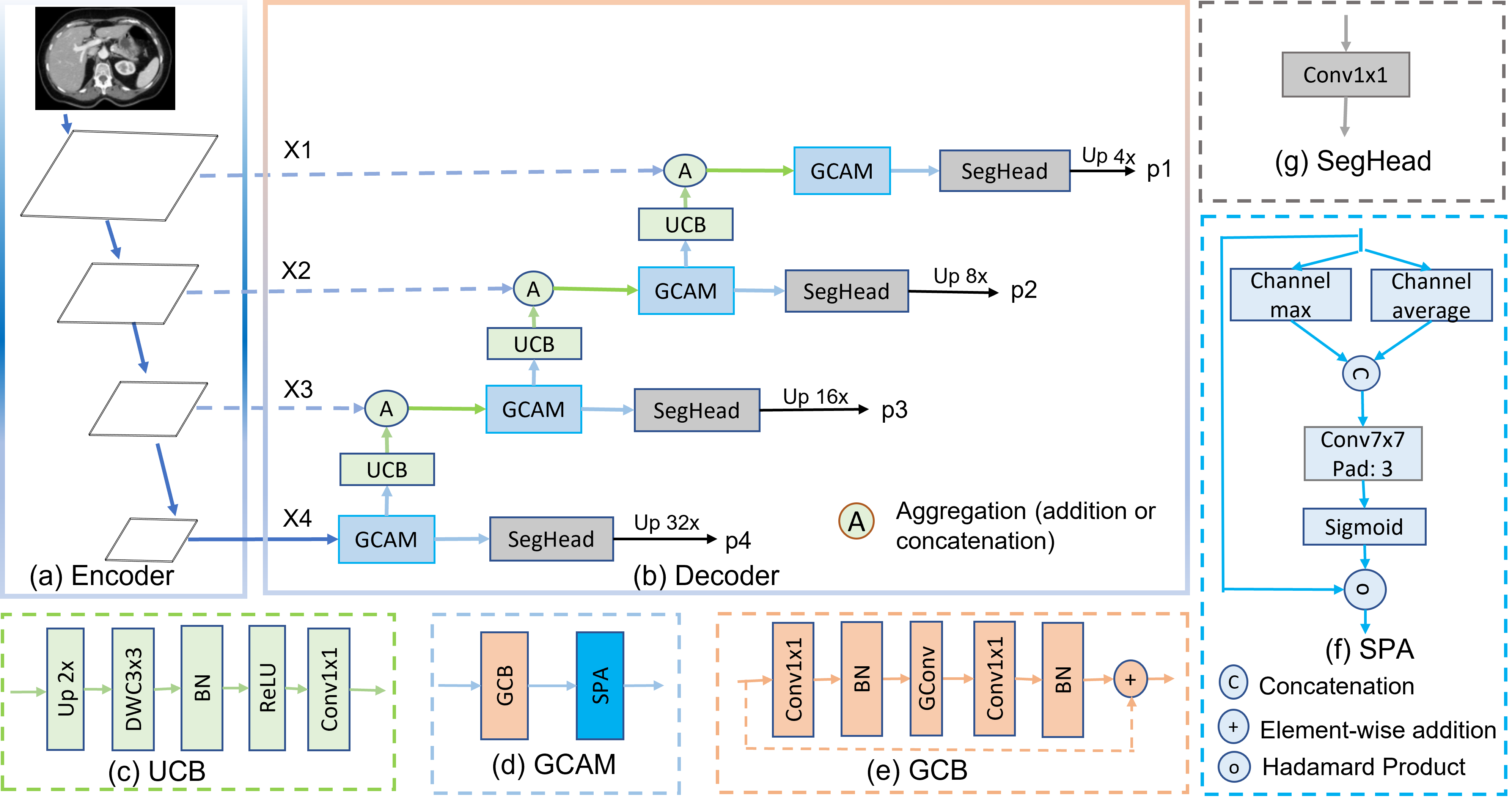
Figure 1: Hierarchical encoder with G-CASCADE network architecture. (a) PVTv2-b2 Encoder backbone with four stages, (b) G-CASCADE decoder, (c) Up-convolution block (UCB), (d) Graph convolutional attention module (GCAM), (e) Graph convolution block (GCB), (f) Spatial attention (SPA), and (g) Segmentation head (SegHead). X1, X2, X3, and X4 are the output features of the four stages of hierarchical encoder. p1, p2, p3, and p4 are output segmentation maps from four stages of our decoder.

2 Related Work

We divide the related work into three parts, i.e., vision transformers, vision graph convolutional networks, and medical image segmentation; these are described next.

2.1 Vision transformers

Dosovitskiy et al. [10] pioneered the development of the vision transformer (ViT), which enables the learning of long-range relationships between pixels through self-attention. Subsequent works have focused on enhancing ViT in various ways, such as integration of convolutional neural networks (CNNs) [40, 34], introducing new SA blocks [23, 34], and novel architectural designs [39, 44]. Liu et al. [23] introduce a sliding window attention mechanism within the hierarchical Swin transformer. Xie et al. [44] present SegFormer, a hierarchical transformer utilizing Mix-FFN blocks. Wang et al. [39] develop the pyramid vision transformer (PVT) with a spatial reduction attention mechanism, and subsequently extend it to PVTv2 [40] by incorporating overlapping patch embedding, a linear complexity attention layer, and a convolutional feed-forward network. Most recently, Tu et al. [34] introduce MaxViT, which employs a multi-axis self-attention mechanism to construct a hierarchical CNN-transformer encoder.

Although vision transformers exhibit remarkable performance, they have certain limitations in their (local) spatial information processing capabilities. In this paper, we aim to overcome these limitations by introducing a new graph-based cascaded attention decoder that preserves the long-range attention through graph convolution and incorporates local attention by a spatial attention mechanism.

2.2 Vision graph convolutional networks

Graph convolutional networks (GCNs) are developed primarily focusing on point clouds classification [20, 21], scene graph generation [45], and action recognition [47] in computer vision. Vision GNN (ViG) [13] introduces the first graph convolutional backbone network to directly process the image data. ViG devides the image into patches and then uses K-nearest neighbors (KNN) algorithm to connect various patches; this enables the processing of long-range dependencies similar to vision transformers. Besides, due to using $1\times 1$ convolutions before and after the graph convolution operation, the graph convolution block used in ViG is significantly faster than the vision transformer and $3\times 3$ convolution-based CNN blocks. Therefore, we propose to use the graph convolution block to decode feature maps for dense prediction. This will make our decoder computationally efficient, while preserving long-range information.

2.3 Medical image segmentation

Medical image segmentation is the task of classifying pixels into lesions, tumours, or organs in a medical image (e.g., endoscopy, MRI, and CT) [4]. To address this task, U-shaped architectures [30, 27, 49, 15, 26] have been commonly utilized due to their sophisticated encoder-decoder structure. Ronneberger et al. [15] introduce UNet, an encoder-decoder architecture that utilizes skip connections to aggregate features from multiple stages. In UNet++ [49], nested encoder-decoder sub-networks are connected through dense skip connections. UNet 3+ [15] further extends this concept by exploring full-scale skip connections with intra-connections among the decoder blocks. DC-UNet [26] incorporates the multi-resolution convolution block and residual path within skip connections. These architectures have proven to be effective in medical image segmentation tasks.

Recently, transformers have gained popularity in the field of medical image segmentation [2, 4, 9, 28, 29, 36, 48]. In TransUNet [4], a hybrid architecture combining CNNs and transformers is proposed to capture both local and global pixel relationships. Swin-Unet [2] adopts a pure U-shaped transformer structure by utilizing Swin transformer blocks [23] in both the encoder and decoder. More recently, Rahman et al. [29] propose a multi-scale hierarchical transformer network with cascaded attention decoding (MERIT) that calculates self attention in varying window sizes to capture effective multi-scale features.

Attention mechanisms have also been explored in combination with both CNNs [27, 11] and transformer-based architectures [9] in medical image segmentation. PraNet [11] utilizes the reverse attention mechanism [6]. In PolypPVT [9], authors employ PVTv2 [40] as the encoder and integrates CBAM [43] attention blocks in the decoder, along with other modules. CASCADE [28] proposes a cascaded decoder that utilizes both channel attention [14] and spatial attention [5] modules for feature refinement. CASCADE extracts features from four stages of the transformer encoder and uses cascaded refinement to generate high-resolution segmentation maps. Due to incorporating local information with global information of transformers, CASCADE exhibits remarkable performance in medical image segmentation. However, CASCADE decoder has two major limitations: this can lead to i) long-range attention deficit due using only convolution operations during decoding and ii) high computational inefficiency due to using three $3\times 3$ convolutions in each stage of the decoder. We propose to use graph convolution to overcome these limitations.

3 Method

In this section, we first introduce a new G-CASCADE decoder, then explain two different transformer-based architectures (i.e., PVT-GCASCADE and MERIT-GCASCADE) incorporating our proposed decoder.

3.1 Cascaded Graph Convolutional Decoder (G-CASCADE)

Existing transformer-based models have limited (local) contextual information processing ability among pixels. As a result, the transformer-based model faces difficulties in locating the more discriminating local features. To address this issue, some works [9, 28, 29] utilize computationally expensive 2D convolution blocks in the decoder. Although the convolution block helps to incorporate the local information, it results in long-range attention deficits. To overcome this problem, we propose a new cascaded graph convolutional decoder, G-CASCADE, for pyramid encoders.

As shown in Figure 1(b), G-CASCADE consists of efficient up-convolution blocks (UCBs) to upsample the features, graph convolutional attention modules (GCAMs) to robustly enhance the feature maps, and segmentation heads (SegHeads) to get the segmentation output. We have four GCAMs for the four stages of pyramid features from the encoder. To aggregate the multi-scale features, we first aggregate (e.g., addition or concatenation) the upsampled features from the previous decoder block with the features from the skip connections. Afterward, we process the concatenated features using our GCAM for enhancing semantic information. We then send the output from each GCAM to a prediction head. Finally, we aggregate four different prediction maps to produce the final segmentation output.

3.1.1 Graph convolutional attention module (GCAM)

We use the graph convolutional attention modules to refine the feature maps. GCAM consists of a graph convolution block ($GCB$(.)) to refine the features preserving long-range attention and a spatial attention [5] ($SPA$(·)) block to capture the local contextual information as in Equation 1:

$$GCAM(x)=SPA(GCB(x))$$ (1)

where $x$ is the input tensor and $GCAM$(·) represents the convolutional attention module. Due to using graph convolution, our GCAM is significantly more efficient than the convolutional attention module (CAM) proposed in [28].

Graph Convolution Block (GCB): The GCB is used to enhance the features generated using our cascaded expanding path. In our GCB, we follow the Grapher design of Vision GNN [13]. GCB consists of a graph convolution layer $GConv$(.) and two $1\times 1$ convolution layers $C$(·) each followed by a batch normalization layer $BN$(·) and a ReLU activation layer $R$(.). $GCB$(·) is formulated as Equation 2:

$$GCB(x)=R(BN(C(GConv(R(BN(C(x)))))))$$ (2)

where $GConv$ can be formulated using Equation 3:

$$GConv(x)=GELU(BN(DynConv(x)))$$ (3)

where $DynConv$(.) is a graph convolution (e.g., max-relative, edge, GraphSAGE, and GIN) in dense dilated K-nearest neighbour (KNN) graph. $BN$(.) and $GELU$(.) are batch normalization and GELU activation, respectively.

SPatial Attention (SPA): The SPA determines where to focus in a feature map; then it enhances those features. The spatial attention is formulated as Equation 4:

$$SPA(x)=Sigmoid(Conv([C_{max}(x),C_{avg}(x)]))\circledast x$$ (4)

where $Sigmoid$(·) is a Sigmoid activation function. $C_{max}$(·) and $C_{avg}$(·) represent the maximum and average values obtained along the channel dimension, respectively. $Conv$(·) is a $7\times 7$ convolution layer with padding $3$ to enhance local contextual information (as in [9]). $\circledast$ is the Hadamard product.

3.1.2 Up-convolution block (UCB)

UCB progressively upsamples the features of the current layer to match the dimension to the next skip connection. Each UCB layer consists of an UpSampling $Up$(·) with scale-factor 2, a $3\times 3$ depth-wise convolution $DWC$(·) with groups equal input channels, a batch normalization $BN$(·), a $ReLU$(.) activation, and a $1\times 1$ convolution $Conv$(.). The $UCB$(·) can be formulated as Equation 5:

$$UCB(x)=Conv(ReLU(BN(DWC(Up(x)))))$$ (5)

Our UCB is light-weight as we replace the $3\times 3$ convolution with a depth-wise convolution after upsampling.

3.1.3 Segmentation head (SegHead)

SegHead takes refined feature maps from the four stages of the decoder as input and predicts four output segmentation maps. Each SegHead layer consists of a $1\times 1$ convolution $Conv_{1\times 1}$(·) which takes feature maps having $N_{i}$ channels ($N_{i}$ is the number of channels in the feature map of stage $i$) as input and gives output with channels equal to number of target classes for multi-class but $1$ channel for binary prediction. The $SegHead$(·) is formulated as Equation 6:

$$SegHead(x)=Conv_{1\times 1}(x)$$ (6)

3.2 Overall architecture

To ensure effective generalization and the ability to process multi-scale features in medical image segmentation, we integrate our proposed G-CASCADE decoder with two different hierarchical backbone encoder networks such as PVTv2 [40] and MERIT [29]. PVTv2 utilizes convolution operations instead of traditional transformer patch embedding modules to consistently capture spatial information. MERIT utilizes two MaxViT [34] encoders with varying window sizes for self-attention, thus enabling the capture of multi-scale features.

By utilizing the PVTv2-b2 (Standard) encoder, we create the PVT-GCASCADE architecture. To adopt PVTv2-b2, we first extract the features (X1, X2, X3, and X4) from four layers and feed them (i.e., X4 in the upsample path and X3, X2, X1 in the skip connections) into our G-CASCADE decoder as shown in Figure 1(a-b). Then, the G-CASCADE processes them and produces four prediction maps that correspond to the four stages of the encoder network.

Besides, we introduce the new MERIT-GCASCADE architecture by adopting the architectural design of the MERIT network. In the case of MERIT, we only replace their decoder with our proposed decoder and keep their hybrid CNN-transformer MaxViT [34] encoder networks. In our MERIT-GCASCADE architecture, we extract hierarchical feature maps from four stages of first encoder and then feed them to the corresponding decoder. Afterwards, we aggregate the feedback from final stage of the decoder to the input image and feed them to second encoder having different window sizes for self-attention. We extract feature maps from four stages of the second decoder and feed them to the second decoder. We send cascaded skip connections like MERIT [29] to the second decoder. We get four output segmentation maps from the four stages of our second decoder. Finally, we aggregate the segmentation maps from the two decoders for four stages separately to produce four output segmentation maps. Our proposed decoder is designed to be adaptable and seamlessly integrates with other hierarchical backbone networks.

3.3 Multi-stage outputs and loss aggregation

We get four output segmentation maps $p_{1}$, $p_{2}$, $p_{3}$, and $p_{4}$ from the four prediction heads for the four stages of our G-CASCADE decoder.

Output segmentation maps aggregation: We compute the final segmentation output using additive aggregation as in Equation 7:

$$seg\_output=\alpha p_{1}+\beta p_{2}+\gamma p_{3}+\zeta p_{4}$$ (7)

where $\alpha$, $\beta$, $\gamma$, and $\zeta$ are the weights of each prediction head. We set $\alpha$, $\beta$, $\gamma$, and $\zeta$ to 1.0 in all our experiments. We get the final prediction output by applying the Sigmoid activation for binary segmentation and Softmax activation for multi-class segmentation.

Loss aggregation: Following MERIT [29], we use the combinatorial loss aggregation strategy, MUTATION in all our experiments. Therefore, we compute the loss for $2^{n}-1$ combinatrorial predictions synthesized from $n$ heads separately and then do a summation of them. We optimize this additive combinatorial loss during training.

Architectures	Average			Aorta	GB	KL	KR	Liver	PC	SP	SM
	DICE$\uparrow$	HD95$\downarrow$	mIoU$\uparrow$
UNet [30]	70.11	44.69	59.39	84.00	56.70	72.41	62.64	86.98	48.73	81.48	67.96
AttnUNet [27]	71.70	34.47	61.38	82.61	61.94	76.07	70.42	87.54	46.70	80.67	67.66
R50+UNet [4]	74.68	36.87	$-$	84.18	62.84	79.19	71.29	93.35	48.23	84.41	73.92
R50+AttnUNet [4]	75.57	36.97	$-$	55.92	63.91	79.20	72.71	93.56	49.37	87.19	74.95
SSFormerPVT [38]	78.01	25.72	67.23	82.78	63.74	80.72	78.11	93.53	61.53	87.07	76.61
PolypPVT [9]	78.08	25.61	67.43	82.34	66.14	81.21	73.78	94.37	59.34	88.05	79.4
TransUNet [4]	77.61	26.9	67.32	86.56	60.43	80.54	78.53	94.33	58.47	87.06	75.00
SwinUNet [2]	77.58	27.32	66.88	81.76	65.95	82.32	79.22	93.73	53.81	88.04	75.79
MT-UNet [37]	78.59	26.59	$-$	87.92	64.99	81.47	77.29	93.06	59.46	87.75	76.81
MISSFormer [16]	81.96	18.20	$-$	86.99	68.65	85.21	82.00	94.41	65.67	91.92	80.81
PVT-CASCADE [28]	81.06	20.23	70.88	83.01	70.59	82.23	80.37	94.08	64.43	90.1	83.69
TransCASCADE [28]	82.68	17.34	73.48	86.63	68.48	87.66	84.56	94.43	65.33	90.79	83.52
Cascaded MERIT [29]	84.32	14.27	75.44	86.67	72.63	87.71	84.62	95.02	70.74	91.98	85.17
PVT-GCASCADE (Ours)	83.28	15.83	73.91	86.50	71.71	87.07	83.77	95.31	66.72	90.84	83.58
MERIT-GCASCADE (Ours)	84.54	10.38	75.83	88.05	74.81	88.01	84.83	95.38	69.73	91.92	83.63

Table 1: Results of Synapse Multi-organ segmentation. We report only DICE scores for individual organs. We get the results of UNet, AttnUNet, PolypPVT, SSFormerPVT, TransUNet, and SwinUNet from [28]. We reproduce the results of Cascaded MERIT with a batch size of 6. $\uparrow$ ($\downarrow$) denotes the higher (lower) the better. G-CASCADE results are averaged over five runs. The best results are shown in bold.

4 Experimental Evaluation

In this section, we first describe the dataset and evaluation metrics followed by implementation details. Then, we conduct a comparative analysis between our proposed G-CASCADE decoder-based architectures and SOTA methods to highlight the superior performance of our approach.

4.1 Datasets

We present the description of Synapse Multi-organ and ACDC datasets below. The description of ISIC2018, polyp, and retinal vessels segmentation datasets are available in supplementary materials (Section A).

Synapse Multi-organ dataset. The Synapse Multi-organ dataset contains 30 abdominal CT scans which have 3779 axial contrast-enhanced slices. Each CT scan has 85-198 slices of $512\times 512$ pixels. Similar to TransUNet [4], we divide the dataset randomly into 18 scans for training (2212 axial slices) and 12 scans for validation. We segment only 8 abdominal organs, i.e., aorta, gallbladder (GB), left kidney (KL), right kidney (KR), liver, pancreas (PC), spleen (SP), and stomach (SM).

ACDC dataset. The ACDC dataset contains 100 cardiac MRI scans each of which consists of three organs, right ventricle (RV), myocardium (Myo), and left ventricle (LV). Following TransUNet [4], we use 70 cases (1930 axial slices) for training, 10 for validation, and 20 for testing.

4.2 Evaluation metrics

We use DICE, mIoU, and 95% Hausdorff Distance (HD95) to evaluate performance on the Synapse Multi-organ dataset. However, for the ACDC dataset, we use only DICE score as an evaluation metrics. We use DICE and mIoU as the evaluation metrics in polyp segmentation and ISIC2018 datasets. The DICE score $DSC(Y,\hat{Y})$, $IoU(Y,\hat{Y})$, and HD95 distance $D_{H}(Y,\hat{Y})$ are calculated using Equations 8, 9, and 10, respectively.

$$DSC(Y,\hat{Y})=\frac{2\times\lvert Y\cap\hat{Y}\rvert}{\lvert Y\rvert+\lvert\hat{Y}\rvert}\times 100$$ (8)

$$IoU(Y,\hat{Y})=\frac{\lvert Y\cap\hat{Y}\rvert}{\lvert Y\cup\hat{Y}\rvert}\times 100$$ (9)

$$\small D_{H}(Y,\hat{Y})=\max\{\max_{y\in Y}\min_{\hat{y}\in\hat{Y}}d(y,\hat{y}),\{\max_{\hat{y}\in\hat{Y}}\min_{y\in Y}d(y,\hat{y})\}$$ (10)

where $Y$ and $\hat{Y}$ are the ground truth and predicted segmentation map, respectively.

4.3 Implementation details

We use Pytorch 1.11.0 to implement our network and conduct experiments. We train all models on a single NVIDIA RTX A6000 GPU with 48GB of memory. We use the PVTv2-b2 and Small CascadedMERIT as representative network. We use the pre-trained weights on ImageNet for both PVT and MERIT backbone networks. We train our model using AdamW optimizer [24] with both learning rate and weight decay of 0.0001.

GCB: We construct dense dilated graph using $K=11$ neighbors for KNN and use the Max-Relative (MR) graph convolution in all our experiments. The batch normalization is used after MR graph convolution. Following ViG [13], we also use the relative position vector for graph construction and reduction ratios of [1, 1, 4, 2] for graph convolution block in different stages.

Synapse Multi-organ dataset. We use a batch size of 6 and train each model for maximum of 300 epochs. We use the input resolution of $224\times 224$ for PVT-GCASCADE and ($256\times 256$, $224\times 224$) for MERIT-GCASCADE. We apply random rotation and flipping for data augmentation. The combined weighted Cross-entropy (0.3) and DICE (0.7) loss are utilized as the loss function.

ACDC dataset. For the ACDC dataset, we train each model for a maximum of 150 epochs with a batch size of 12. We set the input resolution as $224\times 224$ for PVT-GCASCADE and ($256\times 256$, $224\times 224$) for MERIT-GCASCADE. We apply random flipping and rotation for data augmentation. We optimize the combined weighted Cross-entropy (0.3) and DICE (0.7) loss function.

ISIC2018 dataset: We resize the images into $384\times 384$ resolution. Then, we train our model for 200 epochs with a batch size of 4 and a gradient clip of 0.5. We optimize the combined weighted BCE and weighted IoU loss function.

Polyp datasets. We resize the image to $352\times 352$ and use a multi-scale {0.75, 1.0, 1.25} training strategy with a gradient clip limit of 0.5 like CASCADE [28]. We use a batch size of 4 and train each model a maximum of 200 epochs. We optimize the combined weighted BCE and weighted IoU loss function.

Methods Avg Dice RV Myo LV R50+UNet [4] 87.55 87.10 80.63 94.92 R50+AttnUNet [4] 86.75 87.58 79.20 93.47 ViT+CUP [4] 81.45 81.46 70.71 92.18 R50+ViT+CUP [4] 87.57 86.07 81.88 94.75 TransUNet [4] 89.71 86.67 87.27 95.18 SwinUNet [2] 88.07 85.77 84.42 94.03 MT-UNet [37] 90.43 86.64 89.04 95.62 MISSFormer [16] 90.86 89.55 88.04 94.99 PVT-CASCADE [28] 91.46 89.97 88.9 95.50 TransCASCADE [28] 91.63 90.25 89.14 95.50 Cascaded MERIT [29] 91.85 90.23 89.53 95.80 PVT-GCASCADE (Ours) 91.95 90.31 89.63 95.91 MERIT-GCASCADE (Ours) 92.23 90.64 89.96 96.08

Table 2: Results on ACDC dataset. DICE scores are reported for individual organs. We get the results of SwinUNet from [28]. G-CASCADE results are averaged over five runs. The best results are shown in bold.

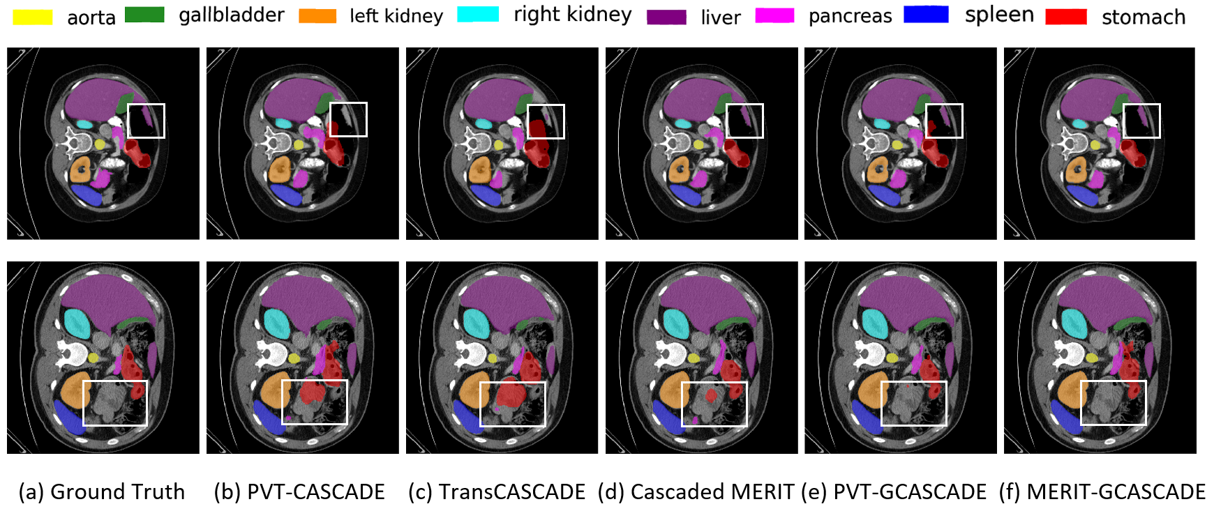
Figure 2: Qualitative results on Synapse multi-organ dataset. (a) Ground Truth (GT), (b) PVT-CASCADE, (c) TransCASCADE, (d) Cascaded MERIT, (e) PVT-GCASCADE, and (f) MERIT-GCASCADE. We overlay the segmentation maps on top of original image/slice. We use the white bounding box to highlight regions where most of the methods have incorrect predictions.

4.4 Results

We compare our architectures (i.e., PVT-GCASCADE and MERIT-GCASCADE) with SOTA CNN and transformer-based segmentation methods on Synapse Multi-organ, ACDC, ISIC2018 [8], and Polyp (i.e., Endoscene [35], CVC-ClinicDB [1], Kvasir [18], ColonDB [32]) datasets. The results of ISIC2018, polyp, and retinal vessels segmentation datasets are reported in the supplementary materials (Section B).

4.4.1 Quantitative results on Synapse Multi-organ dataset

Table 1 presents the performance of different CNN- and transformer-based methods on Synapse Multi-organ segmentation dataset. We can see from Table 1 that our MERIT-GCASCADE significantly outperforms all the SOTA CNN- and transformer-based 2D medical image segmentation methods thus achieving the best average DICE score of 84.54%. Our PVT-GCASCADE and MERIT-GCASCADE outperforms their counterparts PVT-CASCADE and Cascaded MERIT by 2.22% and 0.22% DICE scores, respectively with significantly lower computational costs. Similarly, our PVT-GCASCADE and MERIT-GCASCADE outperforms their counterparts by 4.4 and 3.89 in HD95 distance. Our MERIT-GCASCADE has the lowest HD95 distance (10.38) which is 3.89 lower than the best SOTA method Cascaded MERIT (HD95 of 14.27). The lower HD95 scores indicate that our G-CASCADE decoder can better locate the boundary of organs.

Our proposed decoder also shows boost in the DICE scores of individual organ segmentation. We can see from the Table 1 that our proposed MERIT-GCASCADE significantly outperforms SOTA methods on five out of eight organs. We believe that G-CASCADE decoder demonstrates better performance due to using graph convolution together with the transformer encoder.

4.4.2 Quantitative results on ACDC dataset

We have conducted another set of experiments on the MRI images of the ACDC dataset using our architectures. Table 2 presents the average DICE scores of our PVT-GCASCADE and MERIT-GCASCADE along with other SOTA methods. Our MERIT-GCASCADE achieves the highest average DICE score of 92.23% thus improving about 0.38% over Cascaded MERIT though our decoder has significantly lower computational cost (see Table 5). Our PVT-GCASCADE gains 91.95% DICE score which is also better than all other methods. Besides, both our PVT-GCASCADE and MERIT-GCASCADE have better DICE scores in all three organs segmentation.

4.4.3 Qualitative results on Synapse Multi-organ dataset

We present the segmentation outputs of our proposed method and three other SOTA methods on two sample images in Figure 2. If we look into the highlighted regions in both samples, we can see that MERIT-GCASCADE consistently segments the organs with minimal false negative and false positive results. PVT-GCASCADE and Cascaded MERIT show comparable results. PVT-GCASCADE has false positives in first sample (i.e., first row) and has better segmentation in second sample (i.e., second row), whereas Cascaded MERIT provides better segmentation in first sample but it has larger false positives in second sample. TransCASCADE and PVT-CASCADE provide larger incorrect segmentation outputs in both samples.

Components FLOPs #Params Avg Cascaded GCB SPA (G) (M) DICE No No No 0 0 80.1$\pm$0.2 Yes No No 0.102 0.225 81.1$\pm$0.2 Yes No Yes 0.102 0.225 82.1$\pm$0.3 Yes Yes No 0.341 1.78 83.0$\pm$0.2 Yes Yes Yes 0.342 1.78 83.3$\pm$0.2

Table 3: Quantitative results of different components of G-CASCADE with PVTv2-b2 encoder on Synapse multi-organ dataset. We use additive aggregation for adding skip connections and an input resolution of $224\times 224$ to get these results. All results are averaged over five runs. The best results are showed in bold.

Arrangements	DICE (%)
SPA $\rightarrow$ GCB	82.93$\pm$0.2
GCB $\rightarrow$ SPA (Ours)	83.28$\pm$0.2

Table 4: Comparison of different arrangements of GCB and SPA in GCAM on Synapse Multi-organ dataset. We use PVTv2-b2 as the encoder to produce these results. All the results are averaged over five runs. The best results are in bold.

5 Ablation Study

In this section, we perform a set of ablation experiments that aim to address various questions concerning our proposed architectures and experimental setup. More ablation studies are available in supplementary materials (Section C).

5.1 Effect of different components of G-CASCADE

We carry out ablation studies on the Synapse Multi-organ dataset to evaluate the effectiveness of different components of our proposed G-CASCADE decoder. We use the same PVTv2-b2 backbone pre-trained on ImageNet and the same experimental settings for Synapse Multi-organ dataset in all experiments. We remove different modules such as Cascaded structure, GCB, and SPA from the G-CASCADE decoder and compare the results. It is evident from Table 3 that the cascaded structure of the decoder improves performance over the non-cascaded decoder. GCB and SPA modules also help improve performance. However, the use of both SPA and GCB modules together produces the best DICE score of 83.3%. We can also see from the table that DICE score is improved about 3.2% with 0.342G and 1.78M additional FLOPs and parameters, respectively.

5.2 Effect of arrangements of GCB and SPA in GCAM

We have conducted an ablation study to see the effect of the order of GCB and SPA in GCAM. Table 4 presents the experimental results of two different arrangements. We can conclude from Table 4 that GCB followed by SPA block performs better than SPA followed by GCB. Therefore, in our G-CASCADE decoder, we use a GCB followed by a SPA block in each GCAM.

Decoders UCB FLOPs(G) #Params(M) DICE (%) CASCADE Original 1.93 9.27 82.78 CASCADE Modified 1.22 7.58 82.79 G-CASCADE (Ours) Original 1.06 3.47 83.15 G-CASCADE (Ours) Modified 0.342 1.78 83.28

Table 5: Comparison with the baseline decoder on Synapse Multi-organ dataset. We only report the FLOPs and the number of parameters of the respective decoder. We produce these results using PVTv2-b2 encoder. All the results are averaged over five runs. The best results are in bold.

Architectures Aggregation FLOPs(G) #Params(M) DICE (%) PVT-GCASCADE Addition 0.342 1.78 83.28 PVT-GCASCADE Concat 0.975 3.32 83.40 MERIT-GCASCADE Addition 1.523 3.55 84.54 MERIT-GCASCADE Concat 4.27 5.99 84.63

Table 6: Comparison of different skip-aggregations in G-CASCADE decoder on Synapse Multi-organ dataset. We only report the FLOPs and number of parameters of the respective decoder. PVTV2-b2 encoder has 3.91G FLOPS and 24.86M parameters. Small MERIT encoder has 24.62G FLOPs and 129.38M parameters. All the results are averaged over five runs.

5.3 Comparison with the baseline decoder

Table 5 reports the experimental results with the computational complexity of our baseline CASCADE decoder and our proposed G-CASCADE decoder. We also report the results of original UpConv used in the CASCADE decoder and our modified efficient UCB. From Table 5, we can see that our modified UCB performs equal or better with significantly lower FLOPs and parameters. Our G-CASCADE decoder provides 0.5% better DICE score than the CASCADE decoder with 80.8% fewer parameters and 82.3% fewer FLOPs.

5.4 Effect of different skip-aggregations in G-CASCADE decoder

We conduct some experiments to see the effect of Additive or Concatenation in aggregating upsampled features with the skip-connections. Table 6 presents the results of PVT-GCASCADE and MERIT-GCASCADE with Additive and concatenation aggregations. We can see from Table 6 that Concatenation-based aggregation achieves marginally better DICE scores than Additive aggregation, while having significantly higher FLOPs and parameters. The reason behind this increase in computational complexity is the use of GCAM with the concatenated channels (i.e., 2$\times$ of original channels). Considering the lower computational complexity of Additive aggregation, we have used Additive aggregation in all of our experiments.

6 Conclusion

In this paper, we have introduced a new graph-based cascaded convolutional attention decoder namely G-CASCADE for multi-stage feature aggregation. G-CASCADE enhances feature maps while preserving long-range information captured by transformers which is crucial for accurate medical image segmentation. Due to using graph convolution block instead of $3\times 3$ convolution block, G-CASCADE is computationally efficient. Our experimental results show that G-CASCADE outperforms a recent decoder, CASCADE, in DICE score with 80.8% fewer parameters and 82.3% fewer FLOPs. Our experimental results also demonstrate the superiority of our G-CASCADE decoder over SOTA methods on five public medical image segmentation benchmarks. Finally, we believe that our proposed decoder will improve other downstream medical image segmentation and semantic segmentation tasks.

Methods	Avg
	DICE	mIoU
UNet [30]	85.5	78.5
UNet++ [49]	80.9	72.9
PraNet [11]	87.5	78.7
CaraNet [25]	87.0	78.2
TransUNet [4]	88.0	80.9
TransFuse [48]	90.1	84.0
UCTransNet [36]	90.5	83.0
PolypPVT [9]	91.3	85.2
PVT-CASCADE [28]	91.1	84.9
PVT-GCASCADE (Ours)	91.51$\pm$0.61	86.53$\pm$0.54

Table 7: Results on ISIC2018 dataset. The results of UNet, UNet++, PraNet, CaraNet, TransUNet, TransFuse, UCTransNet, and PolypPVT are taken from [33]. We produce the results of PVT-CASCADE using our experimental settings for this dataset. All PVT-GCASCADE results are averaged over five runs. The best results are in bold.

Methods	CVC-ClinicDB		Kvasir		ColonDB		EndoScene
	DICE	mIoU	DICE	mIoU	DICE	mIoU	DICE	mIoU
UNet [30]	82.3	75.5	81.8	74.6	51.2	44.4	71.0	62.7
UNet++ [49]	79.4	72.9	82.1	74.3	48.3	41.0	70.7	62.4
PraNet [11]	89.9	84.9	89.8	84.0	71.2	64.0	87.1	79.7
CaraNet [25]	93.6	88.7	91.8	86.5	77.3	68.9	90.3	83.8
UACANet-L [19]	91.07	86.7	90.83	85.95	72.57	65.41	88.21	80.84
SSFormerPVT [38]	92.88	88.27	91.11	86.01	79.34	70.63	89.46	82.68
PolypPVT [9]	93.08	88.28	91.23	86.3	80.75	71.85	88.71	81.89
PVT-CASCADE [28]	94.34	89.98	92.58	87.76	82.54	74.53	90.47	83.79
PVT-GCASCADE (Ours)	94.68	90.18	92.74	87.90	82.61	74.60	90.56	83.87

Table 8: Results on polyp segmentation datasets. Training on combined Kvasir [18] and CVC-ClinicDB [1] trainset. The results of UNet, UNet++ and PraNet are taken from [11]. We get the results of PolypPVT, SSFormerPVT, and UACANet from [28]. PVT-GCASCADE results are averaged over five runs. The best results are shown in bold.

Appendix A Datasets

ISIC2018 dataset. ISIC2018 dataset is a skin lesion segmentation dataset [8]. It consists of 2596 images with corresponding annotations. In our experiments, we resize the images to 384 $\times$ 384 resolution unless otherwise mentioned. We randomly split the images into 80% for training, 10% for validation, and 10% for testing.

Polyp datasets. Kvasir contains 1,000 polyp images collected from the polyp class in the Kvasir-SEG dataset [18]. CVC-ClinicDB [1] consists of 612 images extracted from 31 colonoscopy videos. Following CASCADE [28], we adopt the same 900 and 550 images from Kvasir and CVC-ClinicDB, respectively as the training set. We use the remaining 100 and 62 images as the respective testsets. To assess the generalizability of our proposed decoder, we use two unseen test datasets, namely EndoScene [35], and ColonDB [32]. EndoScene and ColonDB consists of 60 and 380 images, respectively.

Retinal vessels segmentation datasets. The DRIVE [31] dataset has 40 retinal images with segmentation annotations. All the retinal images in this dataset are 8-bit color images of resolution $565\times 584$ pixels. The official splits contain a training set of 20 images and a test set of 20 images. The CHASE_DB1 [3] dataset contains 28 color retina images of $999\times 960$ pixels resolution. There are two manual annotations of each image for segmentation. We use the first annotation as the ground truth. Following [22], we use the first 20 images for training, and the remaining 8 images for testing.

Appendix B Experiments

B.1 Implementation details and evaluation metrics

In this subsection, we discuss the implementation details of our proposed decoder for Retinal vessel segmentation. We have conducted experiments on two retinal datasets such as DRIVE [31] and CHASE_DB1 [3]. In both cases, we first extend the training set using horizontal flips, vertical flips, horizontal-vertical flips, random rotations, random colors, and random Gaussian blurs. Through this process, we get 260 images including our 20 original training images. We use 26 of these images for validation that belong to 4 randomly selected original images. In the case of the DRIVE dataset, we resize the images into $768\times 768$ resolution for PVT and ($768\times 768$, $672\times 672$) resolutions for MERIT. In the case of CHASE_DB1, we use $960\times 960$ resolution inputs for PVT and ($768\times 768$, $672\times 672$) resolution inputs for MERIT. However, we resize the output segmentation maps to the original resolution to get evaluation metrics during inference. We use random flips and rotations with a probability of 0.5 as augmentation methods during training. To train our models, we use the AdamW optimizer with both learning rate and weight decay of 1e-4. We optimize the combined weighted BCE and weighted mIoU loss function. The MUTATION is used to aggregate multi-stage loss. We train our networks for 200 epochs with a batch size of 4 and 2 for DRIVE and CHASE_DB, respectively.

We use accuracy (Acc), sensitivity (Sen), specificity (Sp), DICE, and IoU scores as evaluation metrics. We report the percentage (%) score averaging over five runs for both datasets.

B.2 Experimental results on ISIC2018 dataset

Table 7 presents the average DICE scores of our PVT-GCASCADE and MERIT-GCASCADE along with other SOTA methods on the ISIC2018 dataset. This dataset is different than the CT and MRI images used in the above experiments. In this case also, it is evident from the table that our PVT-GCASCADE achieves the best average DICE (91.51%) and mIoU (86.53%) scores. PVT-GCASCADE outperforms its counterpart PVT-CASCADE by 0.4% DICE and 0.6% mIoU scores.

Methods Acc Sen Sp DICE IoU UNet [30] 96.78 80.57 98.33 81.41 68.64 UNet++ [49] 96.79 78.91 98.50 81.14 68.27 Attention UNet [27] 96.62 79.06 98.31 80.39 67.21 FR-UNet [22] 97.05 83.56 98.37 83.16 71.20 PVTV2-b2 (only) [40] 96.24 82.02 97.61 79.14 65.48 PVT-CASCADE [28] 96.79 83.07 98.10 81.73 69.10 MERIT-CASCADE [29] 96.89 82.94 98.22 82.21 69.08 PVT-GCASCADE (Ours) 96.89 83.00 98.22 82.10 69.70 MERIT-GCASCADE (Ours) 97.07 82.81 98.44 82.90 70.81

Table 9: Results (%) of Retinal Vessel Segmentation on DRIVE dataset. The results of UNet, UNet++, Attention UNet, and FR-UNet are taken from [22]. All other results are averaged over five runs in our experimental setups. The best results are in bold.

Methods Acc Sen Sp DICE IoU UNet [30] 97.43 76.50 98.84 78.98 65.26 UNet++ [49] 97.39 83.57 98.32 80.15 66.88 Attention UNet [27] 97.30 83.84 98.20 79.64 66.17 FR-UNet [22] 97.48 87.98 98.14 81.51 68.82 PVTV2-b2 (only) [40] 97.25 85.07 98.07 79.58 66.12 PVT-CASCADE [28] 97.55 85.83 98.34 81.50 68.80 MERIT-CASCADE [29] 97.60 84.97 98.45 81.68 69.06 PVT-GCASCADE (Ours) 97.71 85.84 98.51 82.51 70.24 MERIT-GCASCADE (Ours) 97.76 84.93 98.62 82.67 70.50

Table 10: Results (%) of Retinal Vessel Segmentation on CHASE_DB1 dataset. The results of UNet, UNet++, Attention UNet, and FR-UNet are taken from [22]. All other results are averaged over five runs in our experimental setups. The best results are in bold.

B.3 Experimental results on Polyp datasets

We evaluate the performance and generalizability of our G-CASCADE decoder on four different polyp segmentation testsets among which two are completely unseen datasets collected from different labs. Table 8 displays the DICE and mIoU scores of SOTA methods along with our G-CASCADE decoder. From Table 8, we can see that G-CASCADE significantly outperforms all other methods on both DICE and mIoU scores. It is noteworthy that G-CASCADE outperforms the best CNN-based model UACANet by a large margin on unseen datasets (i.e., 9.8% DICE score improvement in ColonDB). Therefore, we can conclude that due to using transformers as a backbone network and our graph-based convolutional attention decoder, PVT-GCASCADE inherits the merits of transformers, GCNs, CNNs, and local attention which makes them highly generalizable for unseen datasets.

B.4 Experimental results on Retinal vessels segmentation datasets

We have conducted experiments on two retinal vessel segmentation datasets such as DRIVE and CHASE_DB1. The experimental results are reported in Tables 9 and 10. Our G-CASCADE decoder outperforms the baseline CASCADE decoder with significantly lower computational costs. Specifically, our PVT-GCASCADE shows 0.37% and 1.01% improvements in DICE score over PVT-CASCADE in DRIVE and CHASE_DB1 datasets, respectively. Similarly, our MERIT-GCASCADE exhibits 0.69% and 0.99% improvements in DICE score in DRIVE and CHASE_DB1 datasets, respectively. From Tables 9 and 10, we can conclude that our methods show competitive performance compared to the SOTA approaches. Although FR-UNet achieves a 0.26% better DICE score in the DRIVE dataset, it has a 1.16% lower DICE score in CHASE_DB1 than our MERIT-GCASCADE. Besides, FR-UNet splits the retinal images into $48\times 48$ pixels patches in a stride of 6 pixels during training but we use the whole retinal images during both training and inference. Consequently, we have a significantly lower number of samples for training compared to FR-UNet. We can conclude from the results that our G-CASCADE decoder equally performs well in retinal vessel segmentation.

Graph Convolutions FLOPs(G) #Params(M) DICE (%) GIN [46] 0.313 1.59 82.22 EdgeConv [41] 0.957 1.78 82.81 GraphSAGE [12] 0.520 1.88 83.10 Max-Relative [21] (Ours) 0.342 1.78 83.28

Table 11: Experimental results of different graph convolutions in GCAM block on Synapse Multi-organ dataset. We use the PVTV2-b2 encoder and only report the FLOPs and number of parameters of the decoder. All the results are averaged over five runs. The best results are shown in bold.

Architectures FLOPs(G) #Params(M) DICE (%) PVT-CASCADE 5.84 34.13 83.28 PVT-GCASCADE 4.252 26.64 83.40 MERIT-CASCADE 33.31 147.86 84.54 MERIT-GCASCADE 26.143 132.93 84.63

Table 12: Comparison of overall computational complexity. We use the PVTV2-b2 backbone with an input resolution of $224\times 224$ in both PVT-CASCADE and PVT-GCASCADE. We use two Small MaxViT backbones with input resolutions of $256\times 256$ and $224\times 224$ in MERIT architectures.

Input resolutions	DICE (%)	mIoU (%)	HD95 (%)
224$\times$224	83.28	73.91	15.83
256$\times$256	84.21	75.32	14.58
384$\times$384	86.01	78.10	13.67

Table 13: Experimental results of PVT-GCASCADE with different input resolutions on Synapse Multi-organ dataset. All the results are averaged over five runs.

Appendix C Ablation Study

C.1 Comparison among different graph convolutions in GCAM

We report the experimental results of our decoder with different graph convolutions in Table 11. As shown in Table 11, Max-Relative (MR) [21] graph convolution provides the best DICE score (83.28%) with only 0.342G FLOPs and 1.78M parameters. Although GIN [46] has slightly lower FLOPs and parameters, it provides the lowest DICE score (82.22%). EdgeConv [41] and GraphSAGE [12] graph convolutions have lower DICE scores than the MR graph convolution with higher computational costs.

C.2 Overall computational complexity

We report the total parameters and FLOPs of encoder backbones and our decoder in Table 12. We can see from Table 12 that overall computational complexity depends on the number of parameters and FLOPs of the encoder backbones. We implement our decoder on top of PVTV2-b2 [40] and Small MaxViT [34] backbones. Our PVT-GCASCADE has 4.252G FLOPs and 26.64M parameters, which is 1.588G and 7.49M lower than the corresponding PVT-CASCADE architecture. Due to the larger size of two Small MaxViT backbones in MERIT-CASCADE architecture (i.e., 33.31G FLOPs and 147.86M parameters), our MERIT-GCASCADE (i.e., 26.143G FLOPs and 132.93M parameters) is also larger in size. In both cases, the savings in FLOPs and parameters come only from our decoder. Our proposed decoder can easily be plugged into other hierarchical encoders; if a lightweight encoder is used, the total computational cost will be reduced.

C.3 Influence of input resolution

Table 13 presents the quantitative segmentation performance of PVT-GCASCADE network with different input resolutions. We conduct experiments with three input resolutions such as 224$\times$224, 256$\times$256, and 384$\times$384. It is evident from the table that performance improved in all three evaluation metrics for higher input resolutions. We get the best DICE and mIoU 86.01% and 78.10%, respectively with the input resolution of 384$\times$384.

References

- [1] Jorge Bernal, F Javier Sánchez, Gloria Fernández-Esparrach, Debora Gil, Cristina Rodríguez, and Fernando Vilariño. Wm-dova maps for accurate polyp highlighting in colonoscopy: Validation vs. saliency maps from physicians. Computerized Medical Imaging and Graphics, 43:99–111, 2015.
- [2] Hu Cao, Yueyue Wang, Joy Chen, Dongsheng Jiang, Xiaopeng Zhang, Qi Tian, and Manning Wang. Swin-unet: Unet-like pure transformer for medical image segmentation. arXiv preprint arXiv:2105.05537, 2021.
- [3] Adrian Carballal, Francisco J Novoa, Carlos Fernandez-Lozano, Marcos García-Guimaraes, Guillermo Aldama-López, Ramón Calviño-Santos, José Manuel Vazquez-Rodriguez, and Alejandro Pazos. Automatic multiscale vascular image segmentation algorithm for coronary angiography. Biomedical Signal Processing and Control, 46:1–9, 2018.
- [4] Jieneng Chen, Yongyi Lu, Qihang Yu, Xiangde Luo, Ehsan Adeli, Yan Wang, Le Lu, Alan L Yuille, and Yuyin Zhou. Transunet: Transformers make strong encoders for medical image segmentation. arXiv preprint arXiv:2102.04306, 2021.
- [5] Long Chen, Hanwang Zhang, Jun Xiao, Liqiang Nie, Jian Shao, Wei Liu, and Tat-Seng Chua. Sca-cnn: Spatial and channel-wise attention in convolutional networks for image captioning. In Proceedings of the IEEE Conference on Computer Vision and Pattern Recognition (CVPR), pages 5659–5667, 2017.
- [6] Shuhan Chen, Xiuli Tan, Ben Wang, and Xuelong Hu. Reverse attention for salient object detection. In Proceedings of the European Conference on Computer Vision (ECCV), pages 234–250, 2018.
- [7] Xiangxiang Chu, Zhi Tian, Bo Zhang, Xinlong Wang, Xiaolin Wei, Huaxia Xia, and Chunhua Shen. Conditional positional encodings for vision transformers. arXiv preprint arXiv:2102.10882, 2021.
- [8] Noel Codella, Veronica Rotemberg, Philipp Tschandl, M Emre Celebi, Stephen Dusza, David Gutman, Brian Helba, Aadi Kalloo, Konstantinos Liopyris, Michael Marchetti, et al. Skin lesion analysis toward melanoma detection 2018: A challenge hosted by the international skin imaging collaboration (isic). arXiv preprint arXiv:1902.03368, 2019.
- [9] Bo Dong, Wenhai Wang, Deng-Ping Fan, Jinpeng Li, Huazhu Fu, and Ling Shao. Polyp-pvt: Polyp segmentation with pyramid vision transformers. arXiv preprint arXiv:2108.06932, 2021.
- [10] Alexey Dosovitskiy, Lucas Beyer, Alexander Kolesnikov, Dirk Weissenborn, Xiaohua Zhai, Thomas Unterthiner, Mostafa Dehghani, Matthias Minderer, Georg Heigold, Sylvain Gelly, et al. An image is worth 16x16 words: Transformers for image recognition at scale. arXiv preprint arXiv:2010.11929, 2020.
- [11] Deng-Ping Fan, Ge-Peng Ji, Tao Zhou, Geng Chen, Huazhu Fu, Jianbing Shen, and Ling Shao. Pranet: Parallel reverse attention network for polyp segmentation. In International Conference on Medical Image Computing and Computer-Assisted Intervention (MICCAI), pages 263–273. Springer, 2020.
- [12] Will Hamilton, Zhitao Ying, and Jure Leskovec. Inductive representation learning on large graphs. Advances in Neural Information Processing Systems, 30, 2017.
- [13] Kai Han, Yunhe Wang, Jianyuan Guo, Yehui Tang, and Enhua Wu. Vision gnn: An image is worth graph of nodes. arXiv preprint arXiv:2206.00272, 2022.
- [14] Jie Hu, Li Shen, and Gang Sun. Squeeze-and-excitation networks. In Proceedings of the IEEE Conference on Computer Vision and Pattern Recognition (CVPR), pages 7132–7141, 2018.
- [15] Huimin Huang, Lanfen Lin, Ruofeng Tong, Hongjie Hu, Qiaowei Zhang, Yutaro Iwamoto, Xianhua Han, Yen-Wei Chen, and Jian Wu. Unet 3+: A full-scale connected unet for medical image segmentation. In International Conference on Acoustics, Speech and Signal Processing (ICASSP), pages 1055–1059. IEEE, 2020.
- [16] Xiaohong Huang, Zhifang Deng, Dandan Li, and Xueguang Yuan. Missformer: An effective medical image segmentation transformer. arXiv preprint arXiv:2109.07162, 2021.
- [17] Md Amirul Islam, Sen Jia, and Neil DB Bruce. How much position information do convolutional neural networks encode? arXiv preprint arXiv:2001.08248, 2020.
- [18] Debesh Jha, Pia H Smedsrud, Michael A Riegler, Pål Halvorsen, Thomas de Lange, Dag Johansen, and Håvard D Johansen. Kvasir-seg: A segmented polyp dataset. In International Conference on Multimedia Modeling, pages 451–462. Springer, 2020.
- [19] Taehun Kim, Hyemin Lee, and Daijin Kim. Uacanet: Uncertainty augmented context attention for polyp segmentation. In Proceedings of the 29th ACM International Conference on Multimedia, pages 2167–2175, 2021.
- [20] Loic Landrieu and Martin Simonovsky. Large-scale point cloud semantic segmentation with superpoint graphs. In Proceedings of the IEEE Conference on Computer Vision and Pattern Recognition (CVPR), pages 4558–4567, 2018.
- [21] Guohao Li, Matthias Muller, Ali Thabet, and Bernard Ghanem. Deepgcns: Can gcns go as deep as cnns? In Proceedings of the IEEE/CVF International Conference on Computer Vision (ICCV), pages 9267–9276, 2019.
- [22] Wentao Liu, Huihua Yang, Tong Tian, Zhiwei Cao, Xipeng Pan, Weijin Xu, Yang Jin, and Feng Gao. Full-resolution network and dual-threshold iteration for retinal vessel and coronary angiograph segmentation. IEEE Journal of Biomedical and Health Informatics, 26(9):4623–4634, 2022.
- [23] Ze Liu, Yutong Lin, Yue Cao, Han Hu, Yixuan Wei, Zheng Zhang, Stephen Lin, and Baining Guo. Swin transformer: Hierarchical vision transformer using shifted windows. In Proceedings of the IEEE/CVF International Conference on Computer Vision (ICCV), pages 10012–10022, 2021.
- [24] Ilya Loshchilov and Frank Hutter. Decoupled weight decay regularization. arXiv preprint arXiv:1711.05101, 2017.
- [25] Ange Lou, Shuyue Guan, Hanseok Ko, and Murray H Loew. Caranet: context axial reverse attention network for segmentation of small medical objects. In Medical Imaging 2022: Image Processing, volume 12032, pages 81–92. SPIE, 2022.
- [26] Ange Lou, Shuyue Guan, and Murray Loew. Dc-unet: rethinking the u-net architecture with dual channel efficient cnn for medical image segmentation. In Medical Imaging 2021: Image Processing, volume 11596, pages 758–768. SPIE, 2021.
- [27] Ozan Oktay, Jo Schlemper, Loic Le Folgoc, Matthew Lee, Mattias Heinrich, Kazunari Misawa, Kensaku Mori, Steven McDonagh, Nils Y Hammerla, Bernhard Kainz, et al. Attention u-net: Learning where to look for the pancreas. arXiv preprint arXiv:1804.03999, 2018.
- [28] Md Mostafijur Rahman and Radu Marculescu. Medical image segmentation via cascaded attention decoding. In Proceedings of the IEEE/CVF Winter Conference on Applications of Computer Vision (WACV), pages 6222–6231, January 2023.
- [29] Md Mostafijur Rahman and Radu Marculescu. Multi-scale hierarchical vision transformer with cascaded attention decoding for medical image segmentation. In Medical Imaging with Deep Learning, 2023.
- [30] Olaf Ronneberger, Philipp Fischer, and Thomas Brox. U-net: Convolutional networks for biomedical image segmentation. In International Conference on Medical Image Computing and Computer-Assisted Intervention (MICCAI), pages 234–241. Springer, 2015.
- [31] Joes Staal, Michael D Abràmoff, Meindert Niemeijer, Max A Viergever, and Bram Van Ginneken. Ridge-based vessel segmentation in color images of the retina. IEEE transactions on medical imaging, 23(4):501–509, 2004.
- [32] Nima Tajbakhsh, Suryakanth R Gurudu, and Jianming Liang. Automated polyp detection in colonoscopy videos using shape and context information. IEEE Transactions on Medical Imaging, 35(2):630–644, 2015.
- [33] Feilong Tang, Qiming Huang, Jinfeng Wang, Xianxu Hou, Jionglong Su, and Jingxin Liu. Duat: Dual-aggregation transformer network for medical image segmentation. arXiv preprint arXiv:2212.11677, 2022.
- [34] Zhengzhong Tu, Hossein Talebi, Han Zhang, Feng Yang, Peyman Milanfar, Alan Bovik, and Yinxiao Li. Maxvit: Multi-axis vision transformer. In Proceedings of the European Conference on Computer Vision (ECCV), pages 459–479. Springer, 2022.
- [35] David Vázquez, Jorge Bernal, F Javier Sánchez, Gloria Fernández-Esparrach, Antonio M López, Adriana Romero, Michal Drozdzal, and Aaron Courville. A benchmark for endoluminal scene segmentation of colonoscopy images. Journal of Healthcare Engineering, 2017, 2017.
- [36] Haonan Wang, Peng Cao, Jiaqi Wang, and Osmar R Zaiane. Uctransnet: rethinking the skip connections in u-net from a channel-wise perspective with transformer. In Proceedings of the AAAI Conference on Artificial Intelligence, volume 36, pages 2441–2449, 2022.
- [37] Hongyi Wang, Shiao Xie, Lanfen Lin, Yutaro Iwamoto, Xian-Hua Han, Yen-Wei Chen, and Ruofeng Tong. Mixed transformer u-net for medical image segmentation. In International Conference on Acoustics, Speech and Signal Processing (ICASSP), pages 2390–2394. IEEE, 2022.
- [38] Jinfeng Wang, Qiming Huang, Feilong Tang, Jia Meng, Jionglong Su, and Sifan Song. Stepwise feature fusion: Local guides global. arXiv preprint arXiv:2203.03635, 2022.
- [39] Wenhai Wang, Enze Xie, Xiang Li, Deng-Ping Fan, Kaitao Song, Ding Liang, Tong Lu, Ping Luo, and Ling Shao. Pyramid vision transformer: A versatile backbone for dense prediction without convolutions. In Proceedings of the IEEE/CVF International Conference on Computer Vision (ICCV), pages 568–578, 2021.
- [40] Wenhai Wang, Enze Xie, Xiang Li, Deng-Ping Fan, Kaitao Song, Ding Liang, Tong Lu, Ping Luo, and Ling Shao. Pvt v2: Improved baselines with pyramid vision transformer. Computational Visual Media, 8(3):415–424, 2022.
- [41] Yue Wang, Yongbin Sun, Ziwei Liu, Sanjay E Sarma, Michael M Bronstein, and Justin M Solomon. Dynamic graph cnn for learning on point clouds. Acm Transactions On Graphics, 38(5):1–12, 2019.
- [42] Zhendong Wang, Xiaodong Cun, Jianmin Bao, Wengang Zhou, Jianzhuang Liu, and Houqiang Li. Uformer: A general u-shaped transformer for image restoration. In Proceedings of the IEEE/CVF Conference on Computer Vision and Pattern Recognition (CVPR), pages 17683–17693, 2022.
- [43] Sanghyun Woo, Jongchan Park, Joon-Young Lee, and In So Kweon. Cbam: Convolutional block attention module. In Proceedings of the European Conference on Computer Vision (ECCV), pages 3–19, 2018.
- [44] Enze Xie, Wenhai Wang, Zhiding Yu, Anima Anandkumar, Jose M Alvarez, and Ping Luo. Segformer: Simple and efficient design for semantic segmentation with transformers. Advances in Neural Information Processing Systems, 34:12077–12090, 2021.
- [45] Danfei Xu, Yuke Zhu, Christopher B Choy, and Li Fei-Fei. Scene graph generation by iterative message passing. In Proceedings of the IEEE Conference on Computer Vision and Pattern Recognition (CVPR), pages 5410–5419, 2017.
- [46] Keyulu Xu, Weihua Hu, Jure Leskovec, and Stefanie Jegelka. How powerful are graph neural networks? arXiv preprint arXiv:1810.00826, 2018.
- [47] Sijie Yan, Yuanjun Xiong, and Dahua Lin. Spatial temporal graph convolutional networks for skeleton-based action recognition. In Proceedings of the AAAI Conference on Artificial Intelligence, volume 32, 2018.
- [48] Yundong Zhang, Huiye Liu, and Qiang Hu. Transfuse: Fusing transformers and cnns for medical image segmentation. In International Conference on Medical Image Computing and Computer-Assisted Intervention, pages 14–24. Springer, 2021.
- [49] Zongwei Zhou, Md Mahfuzur Rahman Siddiquee, Nima Tajbakhsh, and Jianming Liang. Unet++: A nested u-net architecture for medical image segmentation. In Deep Learning in Medical Image Analysis and Multimodal Learning for Clinical Decision Support, pages 3–11. Springer, 2018.