Astrophysical Parameter Inference on Accreting White Dwarf Binaries using Gravitational Waves

Abstract

Accreting binary white dwarf systems are among the sources expected to emanate gravitational waves that the Laser Interferometer Space Antenna (LISA) will detect. We investigate how accurately the binary parameters may be measured from LISA observations. We complement previous studies by performing our parameter estimation on binaries containing a low-mass donor with a thick, hydrogen-rich envelope. The evolution is followed from the early, pre-period minimum stage, in which the donor is non-degenerate, to a later, post-period minimum stage with a largely degenerate donor. We present expressions for the gravitational wave amplitude, frequency, and frequency derivative in terms of white dwarf parameters (masses, donor radius, etc.), where binary evolution is driven by gravitational wave radiation and accretion torques, and the donor radius and logarithmic change in radius ($\eta_{\rm d}$) due to mass loss are treated as model parameters. We then perform a Fisher analysis to reveal the accuracy of parameter measurements, using models from Modules for Experiments in Stellar Astrophysics (MESA) to estimate realistic fiducial values at which we evaluate the measurement errors. We find that the donor radius can be measured relatively well with LISA observations alone, while we can further measure the individual masses if we have an independent measurement of the luminosity distance from electromagnetic observations. When applied to the parameters of the recently-discovered white dwarf binary ZTF J0127+5258, our Fisher analysis suggests that we will be able to constrain the system’s individual masses and donor radius using LISA’s observations, given ZTF’s measurement of the luminosity distance.

1 Introduction

The first direct detection of gravitational waves (GWs) in 2015 came from the merger of a binary black hole (Abbott et al., 2016). Since then, the LIGO/Virgo Collaborations have additionally detected GW signals from numerous other binary black hole mergers, as well as several binary neutron star and neutron star-black hole mergers (Abbott et al., 2017, 2019, 2021). While LIGO and other ground-based detectors are able to detect GWs with frequencies from about 15 Hz to several kHz  (Abbott et al., 2019), the Laser Interferometer Space Antenna (LISA) is a space-based GW detector expected to launch in the mid-2030s with the ability to detect GWs in the frequency range of $\sim 10^{-4}$ to $10^{-1}$Hz  (Amaro-Seoane et al., 2017). Among the astrophysical sources anticipated to emit GWs within this range are binary white dwarfs (WDs). In fact, for a 4-year observation period, some $\sim 10^{4}$ double white dwarfs (DWDs) are expected to be resolvable with LISA (Lamberts et al., 2019). For DWD systems emitting GWs at relatively high frequency, we anticipate being able to extract significant information from not only the GW frequency but also the GW frequency “chirp," i.e., change in frequency over time ($\dot{f}$) (Shah et al., 2012).

Prospects of measuring astrophysical parameters of detached binary WDs, in particular their individual masses, are studied in Wolz et al. (2021). The authors employ universal relations between the tidal deformability and moment of inertia, and between the moment of inertia and WD mass, to express the finite-size effects entering in the gravitational waveform in terms of the individual masses. By conducting a Fisher analysis on this waveform expressed in terms of the masses, the authors show that LISA will be able to measure individual masses of DWDs for sufficiently small binary separation and large stellar masses.

Accreting DWD systems with close separations can also be strong GW sources (Nelemans et al., 2004). Some of these systems have been observed as cataclysmic variables and are identified as LISA verification sources (Stroeer & Vecchio, 2006; Kupfer et al., 2018). A few examples are V407 Vul (Cropper et al., 1998), HM Cancri (Israel, G. L. et al., 2002; Ramsay et al., 2002), and ES Cet (Warner & Woudt, 2002). The population of these systems depends on the stability of the accretion. The influence of tidal synchronization on the formation of AM Canum Venaticorum (AM CVn) type binaries, a type of DWD system involving accretion of hydrogen-poor gas, has been studied in Marsh et al. (2004); Gokhale et al. (2007); Sepinsky & Kalogera (2014); Kremer et al. (2015). They consider the stability criteria of the accretion, either through a disk or direct impact, taking into account the tidal synchronization torque. Population simulations of such accreting LISA sources have been performed in Kremer et al. (2017); Biscoveanu et al. (2022). In particular, the work by Kremer et al. (2017) demonstrates that $\sim 10^{3}$ DWDs with negative chirp due to accretion may be observed by LISA. In Biscoveanu et al. (2022), they employ a similar population study to further show that LISA is able to constrain the tidal synchronization timescale ($\tau_{0}$) through its influence on the population distribution in the $f$-$\dot{f}$ parameter space. In these studies, they only consider cold degenerate WDs. On the other hand, accreting systems with an extremely low mass WD donor that has a thick hydrogen envelope are studied in Kaplan et al. (2012). These hydrogen-rich donors are what we would expect to see in an early, pre-period minimum stage of binary evolution. Kaplan et al. (2012) highlights the importance of understanding the relative composition of hydrogen and helium in these WDs in order to infer the stability and behavior of the binary. These systems can be candidates of the observed inspiraling cataclysmic variables (e.g., HM Cancri) and may evolve into AM CVn binaries.

In this paper, we investigate the possibility of directly measuring astrophysical parameters of accreting DWDs given LISA’s measurements of the amplitude ($A$), frequency ($f$), and frequency derivative ($\dot{f}$) of GWs emanated by the DWDs. We additionally build on the work of Kaplan et al. (2012) by connecting the non-degenerate regime, in which donor WDs have a lingering hydrogen envelope, with the later, degenerate regime in which the zero-temperature mass-radius relation is valid. We study the evolution of accreting DWDs through the transition between these two regimes. Knowledge of the accretion physics for such DWDs allows us to parameterize their gravitational waveforms in terms of the individual masses and other parameters of interest. We then perform a Fisher analysis on this waveform to determine how well we can constrain the masses and other parameters given LISA’s detections of GWs from accreting DWDs.

We find that with an independent measurement of the luminosity distance of our DWD systems from electromagnetic observations, we are likely to be able to measure the individual masses, donor radius, and exponent of the mass-radius relation given LISA’s measurements of the GW amplitude, frequency, and frequency derivative. With LISA observations alone, we lose our ability to constrain the individual masses, but we are still able to measure the other two parameters.

The rest of the paper is organized as follows. In Sec. 2, we introduce the parameterized gravitational waveform. In Sec. 3, we discuss how the mass-radius relations of our WDs differ in the degenerate versus non-degenerate regimes, introducing models of donors in the non-degenerate regime that we generate with a stellar evolutionary code. We also discuss the dynamical stability of accreting DWDs. Section 4 illustrates the detectability of our DWD systems based on the relative magnitude of these systems’ GW strain versus LISA’s noise curve. Finally, our parameter estimation technique and results are given in Sec. 5, followed by discussion and conclusions in Sec. 6. The geometric units of $c=G=1$ are used in all of our equations, with the physical dimensions being recoverable through the conversion $1M_{\odot}=1.5\mathrm{km}=4.9\times 10^{-6}$s.

2 Gravitational Waveform

The sky-averaged gravitational waveform, $h(t)$, for a DWD with donor mass $m_{\rm d}$ and accretor mass $m_{\rm a}$ is given by

$$h(t)=A\cos\phi(t).$$ (1)

In this expression, $A$ is the amplitude, given by

$$A=\frac{8\mathcal{M}}{5D}(\pi\mathcal{M}f)^{2/3}\,,$$ (2)

where $D$ is the luminosity distance and $\mathcal{M}$ is the chirp mass,

$$\mathcal{M}=\frac{(m_{\rm d}m_{\rm a})^{3/5}}{(m_{\rm d}+m_{\rm a})^{1/5}}.$$ (3)

Assuming a fairly slowly changing GW frequency, so that $\ddot{f}$ and higher derivatives are negligible, the phase $\phi(t)$ is given by (Shah & Nelemans, 2014)

$$\phi(t)=\phi_{0}+2\pi f_{0}\delta t+\pi\dot{f}_{0}\delta t^{2},$$ (4)

where the subscript 0 indicates the quantity measured at the initial time of observation, $t_{0}$, and $\delta t=t-t_{0}$.

Examining Eqs. (2) and (4), it is evident that in order to write the waveform in terms of our parameters of interest, we must express $f$ and $\dot{f}$ in terms of these parameters.

We assume that the semi-major axis, $a$, adjusts itself during accretion such that the donor radius $r_{\rm d}$ always equals the Roche lobe radius, $r_{\rm L}a$, which we approximate with the fitting formula by Eggleton (1983):

$$r_{\rm L}=\frac{0.49q^{2/3}}{0.6q^{2/3}+\ln(1+q^{1/3})},\quad q=\frac{m_{\rm d}}{m_{\rm a}}.$$ (5)

Taking the derivative of $r_{\rm d}=r_{\rm L}a$ leads us to a relation between the mass loss rate and the orbital separation:

$$\frac{\dot{a}}{a}=\frac{\dot{m}_{\rm d}}{m_{\rm d}}(\eta_{\rm d}-\eta_{\rm L}),$$ (6)

where $\eta_{\rm L}$ is the ratio between $\dot{r}_{\rm L}/r_{\rm L}$ and $\dot{m}_{\rm d}/m_{\rm d}$, given by

$$\eta_{\rm L} =\frac{d\ln r_{\rm L}}{d\ln m_{\rm d}}$$ (7)

$$=\Bigl{[}q(1-F)+1\Bigr{]}\frac{2(1+q^{1/3})\ln(1+q^{1/3})-q^{1/3}}{3(1+q^{1/3})\left[0.6q^{2/3}+\ln(1+q^{1/3})\right]},$$

and $\eta_{\rm d}$ is the logarithmic change in radius due to mass loss,

$$\eta_{\rm d}=\frac{d\ln r_{\rm d}}{d\ln m_{\rm d}}.$$ (8)

If $\eta_{\rm d}>0$, the donor shrinks as it loses mass; if $\eta_{\rm d}<0$, as is the case for a degenerate donor, the WD becomes larger in response to mass loss. As in Kaplan et al. (2012), we have introduced the mass-loss fraction, $F$, defined such that $\dot{m}_{\rm a}=-(1-F)\dot{m}_{\rm d}$, to indicate whether the mass transfer is conservative or not. When $F=0$, all mass lost by the donor is gained by the accretor, and there is no overall loss of mass from the binary; $F=1$ indicates that the accreted material is lost by the binary due to stellar winds, classical novae, etc.

We then consider the angular momentum conservation:

$$\dot{J}=\dot{J}_{\mathrm{gr}}+\dot{J}_{\mathrm{acc}},$$ (9)

where $J$ is the orbital angular momentum and $\dot{J}_{\mathrm{gr}}$ is the angular momentum carried away by gravitational radiation,

$$\frac{\dot{J}_{\mathrm{gr}}}{J}=-\frac{32}{5}\frac{Mm_{\rm d}m_{\rm a}}{a^{4}},$$ (10)

with $M=m_{\rm a}+m_{\rm d}$. The “accretion torque", $\dot{J}_{\mathrm{acc}}$, is given by

$$\frac{\dot{J}_{\mathrm{acc}}}{J}=\frac{\dot{m}_{\rm d}}{m_{\rm d}}\sqrt{r_{\rm h}\left(1+q\right)},$$ (11)

where $r_{\rm h}$ is the effective radius (in units of $a$) of material orbiting the accreting companion that carries the same amount of angular momentum as is lost due to the impact.

This accretion torque quantifies the angular momentum lost by the binary when accreted material impacts the companion star directly, rather than forming an accretion disk around the companion. We use a fitting formula for $r_{\rm h}$ that depends only on $q$ (Verbunt & Rappaport, 1988) in the direct impact scenario, and set $r_{\rm h}=0$ for the disk accretion case. To determine whether we have disk accretion or direct impact, we use Eq. (6) of Nelemans et al. (2001) for the definition of the minimum radius,

$$\frac{r_{\rm{min}}}{a} \approx 0.04948-0.03815\,(\log_{10}q)$$ (12)

$$+0.04752\,(\log_{10}q)^{2}-0.006973\,(\log_{10}q)^{3}\,,$$

and assume disk accretion for $r_{\rm a}<r_{\mathrm{min}}$ and direct impact for $r_{\rm a}>r_{\mathrm{min}}$.

For the results shown in Sec. 5, the orbit was always wide enough for a disk to form, allowing us to neglect the torque term. This is because the lingering hydrogen envelopes in our models of donor WDs cause $r_{\rm d}$ (and therefore $r_{\rm{min}}$) to be relatively large, i.e., larger than $r_{\rm a}$.

Kepler’s third law is used to relate $f$, $M$, $r_{\rm d}$ , and $r_{\rm L}$:

$$f=\frac{1}{\pi}\sqrt{\frac{M}{(r_{\rm d}/r_{\rm L})^{3}}}\,.$$ (13)

We find that in the degenerate regime, $f$ calculated according to Eq. (13) depends almost entirely on $m_{\rm d}$, varying very little with different $m_{\rm a}$. This result agrees well with the findings of Breivik et al. (2018) in their analysis of DWDs with degenerate donors (see App. A).

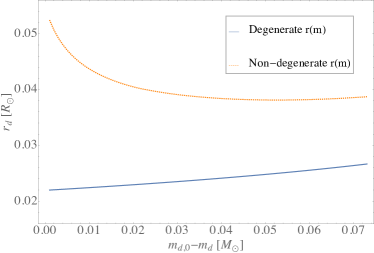
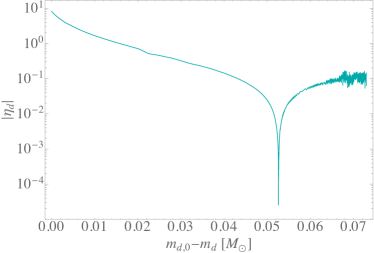
Figure 1: Left: Plot illustrating how the donor’s mass-radius relation differs significantly between degenerate and non-degenerate regimes. As the donor loses mass, the degenerate radius increases steadily ($r_{\rm d}\sim m_{\rm d}^{-1/3}$), whereas the non-degenerate radius (calculated with MESA) first decreases before increasing as the donor becomes increasingly degenerate. Here, the MESA model was computed with a donor having a predominantly helium core of $0.153M_{\odot}$ and initial hydrogen envelope of $0.006M_{\odot}$. Right: $|\eta_{\rm d}|$ vs. stripped mass for the MESA model of a donor. Numerical noise halted the model after about $0.07M_{\odot}$ of mass had been stripped from the donor.

Combining Eqs. (6),  (9),  (10),  (11), and  (13), we now have a full expression for $\dot{f}$:

$$\frac{\dot{f}}{f} =-\frac{16}{5}\frac{Mm_{\rm d}m_{\rm a}}{a^{4}}\times$$ (14)

$$\frac{\frac{Fm_{\rm d}}{M}-3(\eta_{\rm d}-\eta_{\rm L})}{1+q(F-1)-\frac{Fm_{\rm d}}{2M}-r_{\rm h}^{1/2}\left(1+q\right)^{1/2}+\frac{\eta_{\rm d}-\eta_{\rm L}}{2}},$$

i.e., $\dot{f}$ is a function of $m_{\rm d}$, $m_{\rm a}$, $r_{\rm d}$ (through $f$), $\eta_{\rm d}$, and $F$. Notice that one can take the limit of $\eta_{\rm d}-\eta_{\rm L}\to\infty$ in Eq. (14) to find $\dot{a}/a$ and $\dot{f}/f$ without mass accretion. This is because, from Eq. (6), $\dot{m}_{\rm d}$ has to go to 0 when we set $\eta_{\rm d}-\eta_{\rm L}\to\infty$ while keeping $\dot{a}/a$ finite.

The difference from the expressions used in previous work, such as Biscoveanu et al. (2022) (other than the tidal coupling that we do not consider here), is that we (i) introduce the mass-loss fraction $F$ and (ii) further assume $r_{\rm d}=r_{\rm L}a$ at any time so that Eq. (6) holds.

With Eqs. (2),  (4),  (13), and (14), we have a gravitational waveform in terms of the six physical parameters $\phi_{0},m_{\rm d},m_{\rm a},r_{\rm d},\eta_{\rm d}$ and $D$. We use this waveform in our Fisher analysis to determine the measurability of our parameters of interest. We note that despite there being only four raw model parameters in the waveform, $\theta^{i}=(\phi_{0},A,f,\dot{f})$, we can break some of the degeneracy between our six physical parameters by imposing priors on the individual masses (see Sec. 5.1).

3 Astrophysical Properties of Accreting Double White Dwarfs

We now use Modules for Experiments in Stellar Astrophysics (MESA Paxton et al., 2011; Paxton et al., 2013, 2015, 2018, 2019) to study the mass-radius relation and $\eta_{\rm d}$ for WDs and consider the dynamical stability of mass transfer in accreting DWDs.

3.1 Mass-radius Relations

The way in which the donor WD responds to mass loss depends significantly on the composition of the donor. For fully degenerate WDs, we can use Eggleton’s analytic formula to obtain $r_{\rm d}$ in terms of $m_{\rm d}$ (Verbunt & Rappaport, 1988). In this cold temperature regime, $r_{\rm d}$ goes roughly as $m_{\rm d}^{-1/3}$, so $\eta_{\rm d}\sim-1/3$ for a range of $m_{\rm d}$ values.

If the donor is not fully degenerate, $r_{\rm d}$ does not vary with $m_{\rm d}$ in such a simple manner. To reach this conclusion, we used MESA to model mass loss from dozens of WDs containing a range of core and envelope masses. The radius and $\eta_{\rm d}$ of one model are shown in Fig. 1. To construct this model, we used MESA to evolve a $M=$1.5$M_{\odot}$ pre-main sequence star to the red giant branch, and stopped the evolution when the helium core had mass $0.153M_{\odot}$. The hydrogen-rich envelope was then rapidly removed until the envelope was reduced to $0.006M_{\odot}$. In Fig. 1, $|\eta_{\rm d}|$ begins at this point of the simulation; the initial positive value of $\eta_{\rm d}$ reflects the lingering hydrogen envelope surrounding the donor WD. We then simulate mass loss from the donor, causing the WD to become increasingly degenerate as hydrogen is transferred away, resulting in a decreasing $\eta_{\rm d}$ function. Eventually, $\eta_{\rm d}$ passes through zero (seen in the cusp around $0.052M_{\odot}$ of stripped mass). After this point, the donor increases in size as it continues losing mass, causing the orbital separation of the binary to increase.

In the sections that follow, we will use the MESA model described here to obtain realistic fiducial values at which to evaluate the error on the astrophysical parameters, $r_{\rm d}$ and $\eta_{\rm d}$. In so doing, we account for the fact that the accreting DWDs that LISA observes may have low-mass donors with lingering hydrogen envelopes, causing the radius (and $\eta_{\rm d}$) to be larger than what a fully degenerate WD would have. In other words, using the MESA model for fiducial values of $r_{\rm d}$ and $\eta_{\rm d}$ allows us to apply our parameter inference to DWDs in a near-period minimum stage of evolution, when the GW strain is likely to be highest (as we will show in Sec. 4).

Figure 2: The rate of change of GW frequency, $\dot{f}$, for a DWD containing a donor modeled by MESA (mass-radius relation plotted in Fig. 1). Going from right to left on the plot, $\dot{f}$ goes from strictly positive to zero at the dotted white line, to strictly negative.

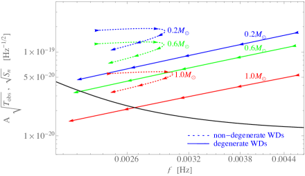
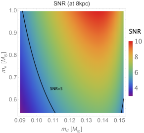
Figure 3: Left: GW strain $(A\times(\mathrm{T_{obs}})^{1/2}$; red, green, blue) and LISA’s noise curve (black) vs. GW frequency for degenerate (solid) and non-degenerate (dashed) DWD systems for a variety of initial accretor masses at a luminosity distance of 8kpc. Arrows show the direction of evolution. The frequency ranges correspond to donor mass ranges of $0.040-0.100M_{\odot}$ and $0.085-0.155M_{\odot}$ for the solid and dashed lines, respectively. Right: The signal-to-noise ratio (SNR) computed for a DWD system with a donor modeled by MESA. The black contour corresponds to SNR=5, which we take as the detection threshold following, e.g., Kremer et al. (2017). Based on these plots, we expect GWs from the DWDs we study to be detectable at distances around 8kpc.

We note that based on Eq. (6), with $\dot{m}_{d}<0$ (donor losing mass), orbital separation will eventually start to grow ($\dot{a}>0$) as $\eta_{\rm d}$ decreases below $\eta_{\rm L}$. In a similar manner, using Eqs. (6) and (14), we see that $\dot{f}$ will also switch from positive to negative as the magnitude of $\eta_{\rm d}$ decreases in comparison with $\eta_{\rm L}$. Figure 2 shows this change of $\dot{f}$ for a binary with a donor mass described by the MESA model in Fig. 1; time evolves from right to left on this plot. All $\dot{f}$ values on the right of the dotted white line (period minimum, where $\dot{f}=0$) are positive, and all values to the left are negative. In this plot, we see a discontinuity in the region between $m_{\rm a}=0.6M_{\odot}$ and $m_{\rm a}=0.7M_{\odot}$. This is due to our choice of a discontinuous transition of $F$ between a region of parameter space in which $F$ equals 0 (lower portion of the plot) to a region in which $F=1$ (upper portion). We will see shortly that our choice of $F$ depends on the magnitude of the accretion rate.

3.2 Dynamical Stability for the DWD systems

The mass transfer process for the DWDs considered here is expected to be unstable for certain mass ratios. Such unstable mass transfer causes dynamical instability of the binary and ultimately results in short-lived DWDs that we do not expect to observe with LISA. We follow Rappaport et al. (1982) in taking mass transfer to be stable if we have a self-consistent solution in Eqs. (6) and (14) assuming $\dot{m}_{\rm d}<0$. Revisiting Eqs. (6) and (14), we arrive at the following criterion for the dynamical stability of the binary:

$$1+q(F-1)-\frac{Fm_{\rm d}}{2M}-r_{\rm h}^{1/2}\left(1+q\right)^{1/2}+\frac{\eta_{\rm d}-\eta_{\rm L}}{2}>0.$$ (15)

From the above expression, it is evident that dynamical stability is dependent on the value of the mass-loss fraction $F$, which is determined by whether the accreted material can be burned stably. We take the criterion for stable hydrogen burning from Kaplan et al. (2012) and adopt

$$F=\begin{cases}1\quad(|\dot{m}_{\rm d}|<\dot{m}_{\mathrm{c}})\,,\\ 0\quad(|\dot{m}_{\rm d}|>\dot{m}_{\mathrm{c}})\,,\end{cases}$$ (16)

where the critical mass loss rate is given by Kaplan et al. (2012),

$$\dot{m}_{\mathrm{c}}=10^{-7}\left(\frac{m_{\rm a}}{M_{\odot}}-0.5357\right)M_{\odot}\,\mathrm{yr}^{-1}\,,$$ (17)

which takes into account the reduced metallicity of the accreting WD.

As mentioned previously, for the results shown in Sec. 5, the orbit was always wide enough for an accretion disk to form. We could then exclude the accretion torque term ($-r_{\rm h}^{1/2}(1+q)^{1/2}$) in Eq. (15), leading to greater dynamical stability (i.e., more regions in which the left-hand side is positive). As mentioned in Kaplan et al. (2012), the hydrogen rich nature of the donor, implying a larger positive $\eta_{\rm d}$, also leads to more dynamical stability.

Lastly, we note that Kaplan et al. (2012) additionally account for the possibility of unstable helium burning at higher mass transfer rates, in which case we could again have $F>0$. It would be interesting to implement a more careful analysis of the different scenarios in which the binaries discussed here might undergo nonconservative mass transfer.

4 GW strain vs. LISA’s Noise Curve

The left panel of Fig. 3 presents the GW strain compared to LISA’s noise curve over a range of GW frequencies. The dashed curves model the GW strain during an earlier stage of DWD evolution (near-period minimum), when the donor has some amount of lingering hydrogen. We construct these curves using Eqs. (2) and (13), along with the mass-radius relation from the MESA model shown in Fig. 1. The solid lines show the GW strain at a much later stage of evolution (post-period minimum), when the donor is fully degenerate and $f$ is steadily decreasing toward the bottom left-hand corner of the plot. These solid curves are constructed using Eggleton’s cold-temperature radius-mass formula (Verbunt & Rappaport, 1988).

We see that in both the early (dashed) and late (solid) stages of evolution of these binaries, the GW strain (plotted as $A\times\mathrm{T_{obs}}^{1/2}$, where $\mathrm{T_{obs}}$ is the observation time that we take to be 4 years) is up to one order of magnitude higher than LISA’s noise curve ($S_{n}(f)$; Robson et al. (2019)). The right panel of Fig. 3 shows the signal-to-noise ratio (SNR) at a luminosity distance of 8kpc. If we follow Kremer et al. (2017) in taking SNR=5 as the minimum SNR for detectability, Fig. 3 confirms that LISA should be able to detect the DWDs discussed here. We note that the GW strain is higher for the non-degenerate case because at the same luminosity distance, a binary with a non-degenerate donor must have a larger donor mass, and therefore chirp mass, to emanate GWs at the same frequency as a comparable binary with a degenerate donor. The larger chirp mass at identical $D$ and $f$ leads to a larger $A$ (see Eq. (2)).

Finally, we note that our calculations for degenerate DWDs in the left panel of Fig. 3 agree well with the SNR results in Fig. 6 of  Kremer et al. (2017). Like them, at D=8kpc and for the mass ranges we consider ($m_{\rm d}\simeq 0.09-0.15M_{\odot},m_{\rm a}\simeq 0.54-1.00M_{\odot}$), we also have a majority of parameter space with SNR between 5 and 10, as well as smaller regions with SNR $<5$ and $\geq 10$.

5 Astrophysical Parameter Inference

Let us now move on to carrying out our parameter estimation for the accreting DWDs with LISA. We first explain our methodology and next present our findings.

5.1 Fisher Method

Given our gravitational waveform derived in Sec. 2, we can estimate the statistical error on parameters due to the detector noise using a Fisher information matrix (FIM) (Cutler, 1998; Shah et al., 2012; Shah & Nelemans, 2014). This method of parameter estimation assumes stationary and Gaussian detector noise.

The FIM is defined as

$$\Gamma_{ij}=\left(\frac{\partial h}{\partial\theta^{i}}\bigg{|}\frac{\partial h}{\partial\theta^{j}}\right)\,,$$ (18)

where the partial derivatives of the waveform $h$ are taken with respect to the parameters of interest described in the previous section,

$$\theta^{i}=(\phi_{0},m_{\rm d},m_{\rm a},r_{\rm d},\eta_{\rm d},D).$$ (19)

The inner product in Eq. (18) is given by

$$(a|b)=4\int^{\infty}_{0}\frac{\tilde{a}^{*}(f)\tilde{b}(f)}{S_{n}(f)}df\approx\frac{2}{S_{n}(f_{0})}\int^{T}_{0}a(t)b(t)dt\,,$$ (20)

with spectral noise density $S_{n}$ and observation time $T$. Tildes indicate Fourier components, and the asterisk denotes the complex conjugate of $\tilde{a}(f)$. We take LISA’s $S_{n}$ from Robson et al. (2019). The monochromatic nature of DWD signals is assumed in our approximation, $S_{n}(f)\approx S_{n}(f_{0})$, and we use Parseval’s theorem to convert the inner product defined in the frequency domain to an integral in the time domain. By inverting the FIM defined in Eq. (18), we obtain the 1-$\sigma$ uncertainty on each of the parameters:

$$\Delta\theta^{i}=\sqrt{(\Gamma^{-1}){}_{ii}}.$$ (21)

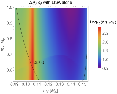
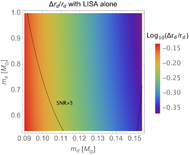
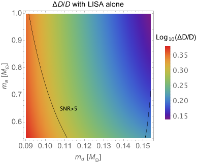
Figure 4: Error on $\eta_{\rm d}$ and fractional error on $r_{\rm d}$ and $D$ for non-degenerate DWD systems, calculated via our Fisher analysis for LISA observations alone. Since inverting the FIM merely returns the priors on the individual masses, giving no new constraints on the mass values, we do not show plots for these parameters. Fiducial values for $\eta_{\rm d}$ and $r_{\rm d}$ were obtained from the MESA model shown in Fig. 1. LISA can detect systems to the right of the black contour corresponding to the detection threshold of SNR=5 (see the right panel of Fig. 3). For the range of parameters shown here, the orbit was wide enough for an accretion disk to form, causing the accretion torque term $-r_{\rm h}^{1/2}(1+q)^{1/2}$ to be zero in Eqs. (14) and (15).

We further impose Gaussian priors on $m_{\rm d}$ and $m_{\rm a}$, with the priors $\sigma_{\theta^{i}}$ defined such that (Poisson & Will, 1995; Cutler & Flanagan, 1994; Carson & Yagi, 2020)

$$\Delta\theta^{i}=\sqrt{(\tilde{\Gamma}^{-1}){}_{ii}}\,,\quad\tilde{\Gamma}_{ij}=\Gamma_{ij}+\frac{1}{\sigma_{\theta^{i}}^{2}}\delta_{ij}.$$ (22)

As previous studies have found that shell flashes occur in the hydrogen envelope of donors with $m_{\rm d}\gtrsim 0.2M_{\odot}$ (Althaus et al., 2001; Panei et al., 2007), we set the prior on the donor to $\sigma_{m_{\rm d}}=0.2M_{\odot}$. Requiring the accretor WD to have a larger mass than the donor WD, we set the prior on the accretor to $\sigma_{m_{\rm a}}=0.8M_{\odot}$, as WDs with masses much higher than $\sim 1.0M_{\odot}$ are less common.

For fiducial values, we take $\phi_{0}=3.666$ rad and $D=8$kpc unless otherwise stated, and vary $(m_{\rm d},m_{\rm a})$. The MESA model in Fig. 1 is used for the fiducial values of $r_{\rm d}(m_{\rm d})$ and $\eta_{\rm d}(m_{\rm d})$. Our results are shown for an observation time of $\mathrm{T_{obs}}=4$ years.

5.2 Results: Gravitational-wave Observations Alone

We begin by presenting results with LISA observations alone. Our parameter set is

$$\theta^{i}=(\phi_{0},m_{\rm d},m_{\rm a},r_{\rm d},\eta_{\rm d},D)\,.$$ (23)

The error on the parameters $\eta_{\rm d},r_{\rm d},$ and $D$ are given in Fig. 4. Unfortunately, in this case, we find that our Fisher analysis merely returns the priors we impose on the masses, i.e., we gain no additional constraints on the individual masses of the DWDs.

Although we are unable to constrain the individual masses with LISA observations alone, there are large regions of parameter space in which the fractional error on $r_{\rm d}$ is smaller than the measurability threshold, $\Delta r_{\rm d}/r_{\rm d}=1$. The same cannot be said for $D$ or $\eta_{\rm d}$; our Fisher analysis suggests that LISA cannot determine these parameters for binaries in consideration.

In the plot of $\Delta\eta_{\rm d}/\eta_{\rm d}$, we see the same discontinuity due to switching $F$ between 0 and 1 that we saw in Fig. 2. The fractional error on $\eta_{\rm d}$ is very large on the left side of the plot, which is partially due to the smallness of the parameter itself (see right panel of Fig. 1). In particular, there is a peak in the fractional error near $m_{\rm d}=0.105M_{\odot}$, corresponding to where $\eta_{\rm d}$ crosses zero, causing $\Delta\eta_{\rm d}/\eta_{\rm d}$ to be very large. However, even all the way to the right of the plot, where $\eta_{\rm d}>1$, the fractional error is generally greater than one, suggesting that we will be unable to constrain $\eta_{\rm d}$ from LISA’s observations.

Let us comment on how the measurement errors on $r_{\rm d}$, $\eta_{\rm d}$, and $D$ scale with $f$, $\dot{f}$ and $A$. We derive the scaling by studying the measurement errors without correlations between parameters. First, we find that the fractional error on $r_{\rm d}$ scales inversely with the signal-to-noise ratio (SNR) times $(df/dr_{\rm d})\times r_{\rm d}$. This is intuitive; we see from Eq. (13) that $f$ depends significantly on $r_{\rm d}$ through the orbital separation, and the error should of course decrease with a larger SNR. The extra factor of $r_{\rm d}$ accounts for the fact that we compare the derivative against our plots of fractional error (i.e., $\Delta r_{\rm d}$ times a factor of $1/r_{\rm d}$). In a similar manner, we find that the error on $\eta_{\rm d}$ scales inversely with SNR$\times(d\dot{f}/d\eta_{\rm d})\times\eta_{\rm d}$, which is sensible, as $\eta_{\rm d}$ only appears in $\dot{f}$ and not $A$ or $f$. Finally, we find that the error on $D$ scales inversely with SNR $\times(dA/dD)\times D$. This is also as we expect; the only place luminosity distance appears in our parameterized gravitational waveform is through the amplitude (Eq. (2)). We note that the clear dependence of $\eta_{\rm d}$, $r_{\rm d}$, and $D$ on $\dot{f}$, $f$, and $A$, respectively, explains the appearance of the discontinuity in the plot of $\eta_{\rm d}$ alone: the mass loss fraction, $F$, only enters the waveform through $\dot{f}$, so the change between $F=0$ and $F=1$ does not alter error calculations on $r_{\rm d}$ and $D$. For more plots and discussion on the scaling of parameter error with various derivatives of the waveform, see App. B.

To summarize, in the absence of an electromagnetic counterpart to LISA’s measurements of accreting DWDs, our Fisher analysis suggests that we will only likely be able to constrain $r_{\rm d}$ out of the six parameters appearing in our gravitational waveform.

5.3 Results: Gravitational-wave Observations with Electromagnetic Counterparts

Let us now consider the case where we have electromagnetic counterparts. A recent paper has shown that at least $\sim 60$ DWDs with helium-rich donors are expected to be observable by both LISA and Gaia (Breivik et al., 2018). For these DWD systems, we can obtain an independent measurement of the luminosity distance $D$ from Gaia. This reduces the number of unknown parameters by one, leaving us with the parameter set

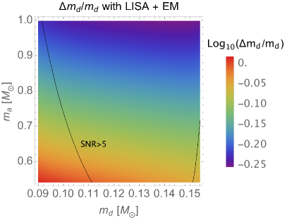
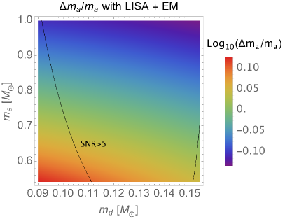
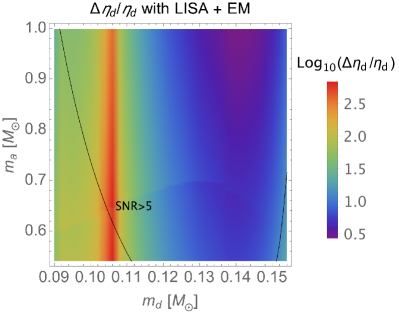
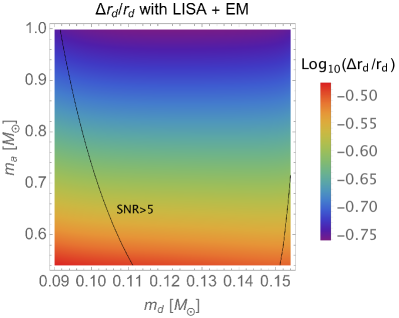
Figure 5: Top row: Fractional error on the individual masses for non-degenerate DWD systems as determined via Fisher analysis using LISA with electromagnetic counterparts. Bottom row, left to right: Error on $\eta_{\rm d}$ and fractional error on $r_{\rm d}$ given by the same Fisher analysis. Fiducial values for $\eta_{\rm d}$ and $r_{\rm d}$ were obtained from the MESA mass-radius relation given in Fig. 1. As in Fig. 4, the accretion torque term was zero in these plots.

$$\theta^{i}=(\phi_{0},m_{\rm d},m_{\rm a},r_{\rm d},\eta_{\rm d}).$$ (25)

Figure 5 shows the measurement uncertainties calculated for the parameters $m_{\rm d}$, $m_{\rm a}$, $\eta_{\rm d},$ and $r_{\rm d},$ as determined via Fisher analysis excluding $D$ as a parameter. We see that if we have an independent measurement of $D$, we can anticipate being able to constrain $m_{\rm d}$ and $m_{\rm a}$ (if $m_{\rm a}$ is sufficiently large for the latter), which we were unable to do without the complementary measurement of $D$. Although the measurability of $\eta_{\rm d}$ does not change significantly, the measurability of $r_{\rm d}$ is considerably enhanced when we perform the Fisher analysis on only five parameters.

Once again, we find that the error (without correlations) on $r_{\rm d}$ and $\eta_{\rm d}$ scales with SNR$\times(df/dr_{\rm d})\times r_{\rm d}$ and SNR$\times(d\dot{f}/d\eta_{\rm d})\times\eta_{\rm d}$, respectively. The errors on $m_{\rm d}$ and $m_{\rm a}$ do not follow such a simple scaling because of the priors that we impose on these parameters. Instead, we find that the error on $m_{\rm a}$ is mainly dominated by the prior, with a slight improvement that comes from the amplitude. On the other hand, the error on $m_{\rm d}$ is determined both from the amplitude and phase.

For the results shown in both Secs. 5.2 and 5.3, we note that the fractional errors on $m_{\rm d}$, $m_{\rm a},$ and $r_{\rm d}$ do not change significantly when we use the MESA model versus Eggleton’s cold-temperature mass-radius relation for fiducial values of $r_{\rm d}$ and $\eta_{\rm d}$. On the other hand, $\Delta\eta_{\rm d}/\eta_{\rm d}$ decreases significantly when we use Eggleton’s mass-radius relation instead of a MESA model for fiducial values. This is because $d\dot{f}/d\eta_{\rm d}$ scales with $r_{\rm d}^{-11/2}$ (see Eqs. (13) and (14), with $r_{\rm d}=r_{\rm L}a$). Evaluating this derivative at the smaller fiducial radius values given by the cold-temperature mass-radius relation (see Fig. 1) causes the Fisher matrix component for $\eta_{\rm d}$, which is determined by $d\dot{f}/d\eta_{\rm d}$, to be larger, leading to a smaller error (from inverting the Fisher matrix).

5.4 Application to ZTF J0127+5258

The discovery of ZTF J0127+5258 was very recently reported (Burdge et al., 2023). This binary system, which has an orbital period of 13.7 minutes, is the first accreting verification DWD system for LISA with a loud enough SNR and luminous donor. The binary is estimated to be at a distance of $3.5^{+1.7}_{-1.5}$kpc with a donor mass of either 0.19$\pm 0.03M_{\odot}$ or 0.31$\pm 0.11M_{\odot}$ and accretor mass of either 0.75$\pm 0.06M_{\odot}$ or 0.87$\pm 0.11M_{\odot}$, depending on the mass transfer rate. Moreover, ZTF J0127+5258 is believed to be a DWD system in the pre-period minimum stage, which would confirm the presence of the DWDs we study within the 8kpc distance we have been considering.

We now show the results of our Fisher analysis method when we apply it to the astrophysical parameters of ZTF J0127+5258. Using the central values of measurements for the masses mentioned in the previous paragraph as fiducial values, along with fiducial $\eta_{\rm d}=1$ and $D=3.5$kpc, our Fisher analysis returns the measurement uncertainties compiled in Table 1. Since we have a measurement of $D$ from ZTF, we perform a Fisher analysis with just the five parameters $(\phi_{0},m_{\rm d},m_{\rm a},r_{\rm d},\eta_{\rm d})$. The resultant calculations of statistical error due to detector noise are relatively small, meaning our constraints of these parameters from GW measurements are likely to be quite strong. We note that with LISA, we can estimate the mass transfer rate from observations. However, the errors on $\dot{m}_{d}$ from LISA’s observations are significant; if we propagate the errors due to $m_{\rm d}$, $m_{\rm a}$, $\eta_{\rm d}$, and $r_{\rm d}$ as listed in Table 1, the propagated error on $\dot{m}_{d}$ overlaps with the standard deviation in mass transfer rate given by Burdge et al. (2023) ($\log(\dot{M}/(M_{\odot}\mathrm{yr}^{-1}))=0.5$). Moreover, the errors we calculate for the individual parameters $m_{\rm d}$, $m_{\rm a}$, and $r_{\rm d}$ overlap with the errors from electromagnetic observations, which also suggests that we will not be able to use LISA’s measurements to identify which of the mass transfer priors reported in Burdge et al. (2023) is more accurate.

	$\mathcal{N}(-8.5,0.5)$	$\mathcal{N}(-7.3,0.5)$
$\Delta m_{\rm d}/m_{\rm d}$	0.6578	0.4921
$\Delta m_{\rm a}/m_{\rm a}$	0.8346	0.5956
$\Delta\eta_{\rm d}/\eta_{\rm d}$	2.6341	0.7218
$\Delta r_{\rm d}/r_{\rm d}$	0.2262	0.1811

Table 1: Measurement uncertainties for astrophysical parameters of ZTF J0127+5258 calculated via our Fisher analysis. The two columns correspond to two sets of fiducial parameter values obtained from different priors of the mass transfer rate, assuming a normal distribution. The priors are denoted by $\mathcal{N}(a,b)$, with $a$ being the center value and $b$ the standard deviation in units of $M_{\odot}\mathrm{yr}^{-1}$. See Burdge et al. (2023) for details.

6 Conclusions

We parameterize the GWs that we expect LISA to detect from accreting DWD systems in terms of the parameters $\theta^{i}=(\phi_{0},m_{\rm d},m_{\rm a},\eta_{\rm d},r_{\rm d},D)$. We perform a Fisher analysis on the parameterized waveform, imposing Gaussian priors on the individual masses based on the properties of the DWDs we expect to be generating the GWs. We find from our Fisher analysis that if we can obtain simultaneous, independent measurements of $D$ from a separate detector like Gaia, then we are likely to be able to constrain not only the individual masses, $m_{\rm d}$ and $m_{\rm a}$, but also $r_{\rm d}$. However, if we use only LISA, lacking an independent measurement of $D$, then although our Fisher analysis still reveals reasonable measurability of $r_{\rm d}$, we lose our ability to constrain the individual masses. Finally, our parameter inference results suggest that we will be able to constrain astrophysical parameters of ZTF J0127+5258 from LISA’s observations of the binary.

Although we found fairly pessimistic results in terms of being able to constrain $\eta_{\rm d}$ itself, we note that our results might nevertheless be useful in distinguishing between the two scenarios of a hydrogen-rich donor ($\eta_{\rm d}\gtrsim 1$) versus a cold, degenerate donor ($\eta_{\rm d}\approx-1/3$). To see this, we note that the errors obtained by Fisher analysis are interpreted as the standard deviation, $\sigma$, of a normal distribution centered at the best fit parameter. Given a fiducial $\eta_{\rm{d,fid}}$, we can therefore use our results to investigate the probability that $\eta_{\rm d}$ is in some range $\eta_{\rm{d,min}}-\eta_{\rm{d,max}}$, i.e.,

$$\int_{\eta_{\rm{d,min}}}^{\eta_{\rm{d,max}}}P(\eta_{\rm d})d\eta_{\rm d},$$ (26)

where $P(\eta_{\rm d})=\mathcal{N}(\eta_{\rm{d,fid}},\sigma)$. In particular, for a given $\eta_{\rm{d,fid}}$, we can integrate the distribution from $-\infty$ to $-1/3$ to reveal the probability that the donor WD is in the late (T=0) stage of evolution with $\eta_{\rm d}<-1/3$. Repeating the above prescription with $r_{\rm d}$ instead of $\eta_{\rm d}$ would similarly allow us to distinguish between a finite temperature WD (with a larger radius) and a cold WD (with a smaller radius). Collectively, the distributions for $\eta_{\rm d}$ and $r_{\rm d}$ obtained from our Fisher analysis could lend insight into what stage of evolution the DWDs are in when we observe them with LISA. We leave this for a future extension of this study.

There are a few additional avenues for future work to improve the current analysis. First, we have only used one evolutionary model of a hydrogen-rich donor to estimate errors on the physical parameters of all DWDs with such donors that LISA will observe. To test the robustness of this analysis, one should study how much $\eta_{\rm d}$ can vary as a function of $m_{\rm d}$ between different hydrogen-rich donors, and see whether this variability affects our parameter inference. It would also be interesting to confirm and generalize our findings using a full Bayesian Markov-chain Monte-Carlo analysis (Cornish & Littenberg, 2007). One can also include the effect of tidal synchronization torque, as done in Biscoveanu et al. (2022); Kremer et al. (2015); Kremer et al. (2017).

Appendix A Corroboration of the $m_{\rm d}-f$ relation for negatively chirping DWD systems

In a previous work, Breivik et al. (2018) report nearly identical evolutionary tracks of $m_{\rm d}$ versus $f$ in their simulations of several thousand negatively chirping DWDs containing low-mass helium core donors. They fit the relation between $m_{\rm d}$ and $f$ to a fourth-order polynomial shown in the top panel of Fig. 6. In the same figure, we plot tracks of $m_{\rm d}$ versus $f$ calculated via Eq. (13), using Eggleton’s cold-temperature mass-radius relation to obtain donor radius values (Verbunt & Rappaport, 1988). It is evident that despite the accretor mass appearing in the total mass in Eq. (13), the evolution of $m_{\rm d}$ with $f$ is largely insensitive to the mass of the accreting companion in the negatively chirping regime; the fractional difference between our relations with different $m_{\rm a}$ values and the analytic fit is less than 8% (see the bottom panel of Fig. 6). For DWDs containing low-mass degenerate donors, our analytic calculation of $f$ agrees excellently with the analytic fit in Eq. (1) of Breivik et al. (2018).

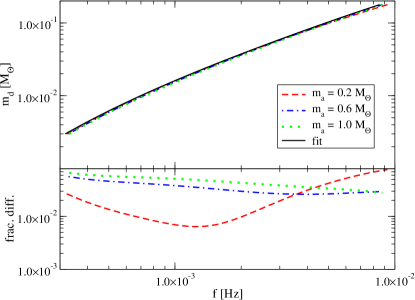
Figure 6: Top: Our evolutionary tracks of $m_{\rm d}$ vs. $f$ for low-mass degenerate donors and various $m_{\rm a}$, as well as the analytic fit for similar DWD systems studied in Breivik et al. (2018). Bottom: Fractional difference between each $f$-$m_{\rm d}$ relation and the fit.

Appendix B Further Analysis on Parameter Estimation Results

In Secs. 5.2 and 5.3, we mention the inverse scaling of the error on $r_{\rm d}$ and $\eta_{\rm d}$ with the SNR times $df/dr_{\rm d}$ and $d\dot{f}/d\eta_{\rm d}$, respectively. In Sec. 5.2, we additionally find that the error on $D$ scales inversely with SNR$\times dA/dD$. To illustrate this point, we plot in Fig. 7 the error on each of these parameters (without correlations) alongside the partial derivative of the waveform with which the error scales. We only show plots for the case of LISA observations alone (i.e., the six-parameter case including $D$ as a Fisher parameter), as the scaling of the error on $\eta_{\rm d}$ and $r_{\rm d}$ works much the same way for both the five- and six-parameter cases. We note that each panel on the left column has a similar structure to the corresponding panel on the right column (color codings are opposite because one scales inversely with the other).

Based on Fig. 7, we see that $r_{\rm d}$ is largely determined by $f$, $\eta_{\rm d}$ is determined by $\dot{f}$, and $D$ is determined by $A$. The latter two statements are not surprising; $\eta_{\rm d}$ and $D$ only appear in the waveform through $\dot{f}$ and $A$, respectively, so we would not expect the error on these parameters to be affected by anything else (other than the SNR). The clear scaling of $r_{\rm d}$ with $f$ is slightly less trivial since $r_{\rm d}$ technically appears in all three pieces of the waveform, $A$, $f$, and $\dot{f}$. However, since $r_{\rm d}$ only enters the amplitude and $\dot{f}$ through $f$, we should not ultimately be surprised that $r_{\rm d}$ scales most strongly with just the GW frequency (and SNR).

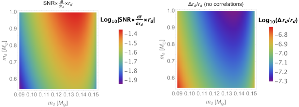
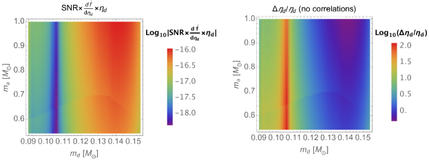
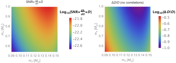
Figure 7: Plots illustrating how errors on $r_{\rm d}$, $\eta_{\rm d}$, and $D$ (right) depend most heavily on the SNR and $f,\dot{f},$ and $A$, respectively (left).

References

- Abbott et al. (2016) Abbott B. P., et al., 2016, Phys. Rev. Lett., 116, 061102
- Abbott et al. (2017) Abbott B. P., et al., 2017, Phys. Rev. Lett., 119, 161101
- Abbott et al. (2019) Abbott B. P., et al., 2019, Phys. Rev. X, 9, 031040
- Abbott et al. (2021) Abbott R., et al., 2021, ApJL, 915, L5
- Althaus et al. (2001) Althaus L. G., Serenelli A. M., Benvenuto O. G., 2001, MNRAS, 323, 471
- Amaro-Seoane et al. (2017) Amaro-Seoane P., et al., 2017, preprint (arXiv:1702.00786)
- Biscoveanu et al. (2022) Biscoveanu S., Kremer K., Thrane E., 2022, arXiv e-prints, p. arXiv:2206.15390
- Breivik et al. (2018) Breivik K., Kremer K., Bueno M., Larson S. L., Coughlin S., Kalogera V., 2018, ApJL, 854, L1
- Burdge et al. (2023) Burdge K. B., et al., 2023, ApJL, 953, L1
- Carson & Yagi (2020) Carson Z., Yagi K., 2020, Phys. Rev. D, 101, 044047
- Cornish & Littenberg (2007) Cornish N. J., Littenberg T. B., 2007, Phys. Rev. D, 76, 083006
- Cropper et al. (1998) Cropper M., Harrop-Allin M. K., Mason K. O., Mittaz J. P. D., Potter S. B., Ramsay G., 1998, MNRAS, 293, L57
- Cutler (1998) Cutler C., 1998, Phys. Rev. D, 57, 7089
- Cutler & Flanagan (1994) Cutler C., Flanagan É. E., 1994, Phys. Rev. D, 49, 2658
- Eggleton (1983) Eggleton P. P., 1983, ApJ, 268, 368
- Gokhale et al. (2007) Gokhale V., Peng X. M., Frank J., 2007, ApJ, 655, 1010
- Israel, G. L. et al. (2002) Israel, G. L. et al., 2002, A&A, 386, L13
- Kaplan et al. (2012) Kaplan D. L., Bildsten L., Steinfadt J. D. R., 2012, ApJ, 758, 64
- Kremer et al. (2015) Kremer K., Sepinsky J., Kalogera V., 2015, ApJ, 806, 76
- Kremer et al. (2017) Kremer K., Breivik K., Larson S. L., Kalogera V., 2017, ApJ, 846, 95
- Kupfer et al. (2018) Kupfer T., et al., 2018, MNRAS, 480, 302
- Lamberts et al. (2019) Lamberts A., Blunt S., Littenberg T. B., Garrison-Kimmel S., Kupfer T., Sanderson R. E., 2019, MNRAS, 490, 5888
- Marsh et al. (2004) Marsh T. R., Nelemans G., Steeghs D., 2004, MNRAS, 350, 113
- Nelemans et al. (2001) Nelemans G., Portegies Zwart S. F., Verbunt F., Yungelson L. R., 2001, A&A, 368, 939
- Nelemans et al. (2004) Nelemans G., Yungelson L. R., Portegies Zwart S. F., 2004, MNRAS, 349, 181
- Panei et al. (2007) Panei J. A., Althaus L. G., Chen X., Han Z., 2007, MNRAS, 382, 779
- Paxton et al. (2011) Paxton B., Bildsten L., Dotter A., Herwig F., Lesaffre P., Timmes F., 2011, ApJS, 192, 3
- Paxton et al. (2013) Paxton B., et al., 2013, ApJS, 208, 4
- Paxton et al. (2015) Paxton B., et al., 2015, ApJS, 220, 15
- Paxton et al. (2018) Paxton B., et al., 2018, ApJS, 234, 34
- Paxton et al. (2019) Paxton B., et al., 2019, ApJS, 243, 10
- Poisson & Will (1995) Poisson E., Will C. M., 1995, Phys. Rev. D, 52, 848
- Ramsay et al. (2002) Ramsay G., Hakala P., Cropper M., 2002, MNRAS, 332, L7
- Rappaport et al. (1982) Rappaport S., Joss P., Webbink R., 1982, ApJ, 254, 616
- Robson et al. (2019) Robson T., Cornish N. J., Liu C., 2019, Classical Quantum Gravity, 36, 105011
- Sepinsky & Kalogera (2014) Sepinsky J. F., Kalogera V., 2014, ApJ, 785, 157
- Shah & Nelemans (2014) Shah S., Nelemans G., 2014, ApJ, 791, 76
- Shah et al. (2012) Shah S., van der Sluys M., Nelemans G., 2012, A&A, 544, A153
- Stroeer & Vecchio (2006) Stroeer A., Vecchio A., 2006, Classical and Quantum Gravity, 23, S809
- Verbunt & Rappaport (1988) Verbunt F., Rappaport S., 1988, ApJ, 332, 193
- Warner & Woudt (2002) Warner B., Woudt P. A., 2002, PASP, 114, 129
- Wolz et al. (2021) Wolz A., Yagi K., Anderson N., Taylor A. J., 2021, MNRAS, 500, L52