A high order accurate bound-preserving compact finite difference scheme for scalar convection diffusion equations

Abstract

We show that the classical fourth order accurate compact finite difference scheme with high order strong stability preserving time discretizations for convection diffusion problems satisfies a weak monotonicity property, which implies that a simple limiter can enforce the bound-preserving property without losing conservation and high order accuracy. Higher order accurate compact finite difference schemes satisfying the weak monotonicity will also be discussed.

65M06, 65M12

1 Introduction

1.1 The bound-preserving property

Consider the initial value problem for a scalar convection diffusion equation $u_{t}+f(u)_{x}=a(u)_{xx},\quad u(x,0)=u_{0}(x),$ where $a^{\prime}(u)\geq 0$. Assume $f(u)$ and $a(u)$ are well-defined smooth functions for any $u\in[m,M]$ where $m=\min_{x}u_{0}(x)$ and $M=\max_{x}u_{0}(x)$. Its exact solution satisfies:

(1) $$\min_{x}u_{0}(x)=m\leq u(x,t)\leq M=\max_{x}u_{0}(x),\quad\forall t\geq 0.$$

In this paper, we are interested in constructing a high order accurate finite difference scheme satisfying the bound-preserving property (1).

For a scalar problem, it is desired to achieve (1) in numerical solutions mainly for the physical meaning. For instance, if $u$ denotes density and $m=0$, then negative numerical solutions are meaningless. In practice, in addition to enforcing (1), it is also critical to strictly enforce the global conservation of numerical solutions for a time-dependent convection dominated problem. Moreover, the computational cost for enforcing (1) should not be significant if it is needed for each time step.

1.2 Popular methods for convection problems

For the convection problems, i.e., $a(u)\equiv 0$, a straightforward way to achieve the above goals is to require a scheme to be monotone, total-variational-diminishing (TVD), or satisfying a discrete maximum principle, which all imply the bound-preserving property. But most schemes satisfying these stronger properties are at most second order accurate. For instance, a monotone scheme and traditional TVD finite difference and finite volume schemes are at most first order accurate [7]. Even though it is possible to have high order TVD finite volume schemes in the sense of measuring the total variation of reconstruction polynomials [12, 22], such schemes can be constructed only for the one-dimensional problems. The second order central scheme satisfies a discrete maximum principle $\min_{j}u_{j}^{n}\leq u_{j}^{n+1}\leq\max_{j}u_{j}^{n}$ where $u^{n}_{j}$ denotes the numerical solution at $n$-th time step and $j$-th grid point [8]. Any finite difference scheme satisfying such a maximum principle can be at most second order accurate, see Harten’s example in [24]. By measuring the extrema of reconstruction polynomials, third order maximum-principle-satisfying schemes can be constructed [9] but extensions to multi-dimensional nonlinear problems are very difficult.

For constructing high order accurate schemes, one can enforce only the bound-preserving property for fixed known bounds, e.g., $m=0$ and $M=1$ if $u$ denotes the density ratio. Even though high order linear schemes cannot be monotone, high order finite volume type spatial discretizations including the discontinuous Galerkin (DG) method satisfy a weak monotonicity property [23, 24, 25]. Namely, in a scheme consisting of any high order finite volume spatial discretization and forward Euler time discretization, the cell average is a monotone function of the point values of the reconstruction or approximation polynomial at Gauss-Lobatto quadrature points. Thus if these point values are in the desired range $[m,M]$, so are the cell averages in the next time step. A simple and efficient local bound-preserving limiter can be designed to control these point values without destroying conservation. Moreover, this simple limiter is high order accurate, see [23] and the appendix in [20]. With strong stability preserving (SSP) Runge-Kutta or multistep methods [4], which are convex combinations of several formal forward Euler steps, a high order accurate finite volume or DG scheme can be rendered bound-preserving with this limiter. These results can be easily extended to multiple dimensions on cells of general shapes. However, for a general finite difference scheme, the weak monotonicity does not hold.

For enforcing only the bound-preserving property in high order schemes, efficient alternatives include a flux limiter [19, 18] and a sweeping limiter in [10]. These methods are designed to directly enforce the bounds without destroying conservation thus can be used on any conservative schemes. Even though they work well in practice, it is nontrivial to analyze and rigorously justify the accuracy of these methods especially for multi-dimensional nonlinear problems.

1.3 The weak monotonicity in compact finite difference schemes

Even though the weak monotonicity does not hold for a general finite difference scheme, in this paper we will show that some high order compact finite difference schemes satisfy such a property, which implies a simple limiting procedure can be used to enforce bounds without destroying accuracy and conservation.

To demonstrate the main idea, we first consider a fourth order accurate compact finite difference approximation to the first derivative on the interval $[0,1]$:

$$\frac{1}{6}(f^{\prime}_{i+1}+4f^{\prime}_{i}+f^{\prime}_{i-1})=\frac{f_{i+1}-f_{i-1}}{2\Delta x}+\mathcal{O}(\Delta x^{4}),$$

where $f_{i}$ and $f^{\prime}_{i}$ are point values of a function $f(x)$ and its derivative $f^{\prime}(x)$ at uniform grid points $x_{i}$ $(i=1,\cdots,N)$ respectively. For periodic boundary conditions, the following tridiagonal linear system needs to be solved to obtain the implicitly defined approximation to the first order derivative:

(2) $$\frac{1}{6}\begin{pmatrix}4&1&&&1\\ 1&4&1&&\\ &\ddots&\ddots&\ddots&\\ &&1&4&1\\ 1&&&1&4\\ \end{pmatrix}\begin{pmatrix}f^{\prime}_{1}\\ f^{\prime}_{2}\\ \vdots\\ f^{\prime}_{N-1}\\ f^{\prime}_{N}\end{pmatrix}=\frac{1}{2\Delta x}\begin{pmatrix}0&1&&&-1\\ -1&0&1&&\\ &\ddots&\ddots&\ddots&\\ &&-1&0&1\\ 1&&&-1&0\\ \end{pmatrix}\begin{pmatrix}f_{1}\\ f_{2}\\ \vdots\\ f_{N-1}\\ f_{N}\end{pmatrix}.$$

We refer to the tridiagonal $\frac{1}{6}(1,4,1)$ matrix as a weighting matrix. For the one-dimensional scalar conservation laws with periodic boundary conditions on $[0,1]$:

(3) $$u_{t}+f(u)_{x}=0,\quad u(x,0)=u_{0}(x),$$

the semi-discrete fourth order compact finite difference scheme can be written as

(4) $$\frac{d\bar{u}_{i}}{dt}=-\frac{1}{2\Delta x}[f(u_{i+1})-f(u_{i-1})],$$

where $\bar{u}_{i}$ is defined as $\bar{u}_{i}=\frac{1}{6}(u_{i-1}+4u_{i}+u_{i+1}).$ Let $\lambda=\frac{\Delta t}{\Delta x}$, then (4) with the forward Euler time discretization becomes

(5) $$\bar{u}_{i}^{n+1}=\bar{u}_{i}^{n}-\frac{1}{2}\lambda[f(u^{n}_{i+1})-f(u^{n}_{i-1})].$$

The following weak monotonicity holds under the CFL $\lambda\max_{u}|f^{\prime}(u)|\leq\frac{1}{3}$:

$$\bar{u}^{n+1}_{i} =\frac{1}{6}(u^{n}_{i-1}+4u^{n}_{i}+u^{n}_{i+1})-\frac{1}{2}\lambda[f(u^{n}_{i+1})-f(u^{n}_{i-1})]$$

$$=\frac{1}{6}[u_{i-1}+3\lambda f(u^{n}_{i-1})]+\frac{1}{6}[u^{n}_{i+1}-3\lambda f(u^{n}_{i+1})]+\frac{4}{6}u^{n}_{i}$$

$$=H(u^{n}_{i-1},u^{n}_{i},u^{n}_{i+1})=H(\uparrow,\uparrow,\uparrow),$$

where $\uparrow$ denotes that the partial derivative with respect to the corresponding argument is non-negative. Therefore $m\leq u^{n}_{i}\leq M$ implies $m=H(m,m,m)\leq\bar{u}^{n+1}_{i}\leq H(M,M,M)=M,$ thus

(6) $$m\leq\frac{1}{6}(u^{n+1}_{i-1}+4u^{n+1}_{i}+u^{n+1}_{i+1})\leq M.$$

If there is any overshoot or undershoot, i.e., $u^{n+1}_{i}>M$ or $u^{n+1}_{i}<m$ for some $i$, then (6) implies that a local limiting process can eliminate the overshoot or undershoot. Here we consider the special case $m=0$ to demonstrate the basic idea of this limiter, and for simplicity we ignore the time step index $n+1$. In Section 2 we will show that $\frac{1}{6}(u_{i-1}+4u_{i}+u_{i+1})\geq 0,\forall i$ implies the following two facts:

1. $\max\{u_{i-1},u_{i},u_{i+1}\}\geq 0;$

2. If $u_{i}<0$, then $\frac{1}{2}(u_{i-1})_{+}+\frac{1}{2}(u_{i+1})_{+}\geq-u_{i}>0$, where $(u)_{+}=\max\{u,0\}.$

By the two facts above, when $u_{i}<0$, then the following three-point stencil limiting process can enforce positivity without changing $\sum_{i}u_{i}$:

$$v_{i-1}=u_{i-1}+\frac{(u_{i-1})_{+}}{(u_{i-1})_{+}+(u_{i+1})_{+}}u_{i};\quad v_{i+1}=u_{i+1}+\frac{(u_{i+1})_{+}}{(u_{i-1})_{+}+(u_{i+1})_{+}}u_{i},$$

$$\text{replace}\quad u_{i-1},\,u_{i},\,u_{i+1}\quad\text{by}\quad v_{i-1},\,0,\,v_{i+1}\quad\textrm{respectively}.$$

In Section 2.2, we will show that such a simple limiter can enforce the bounds of $u_{i}$ without destroying accuracy and conservation. Thus with SSP high order time discretizations, the fourth order compact finite difference scheme solving (3) can be rendered bound-preserving by this limiter. Moreover, in this paper we will show that such a weak monotonicity and the limiter can be easily extended to more general and practical cases including two-dimensional problems, convection diffusion problems, inflow-outflow boundary conditions, higher order accurate compact finite difference approximations, compact finite difference schemes with a total-variation-bounded (TVB) limiter [3]. However, the extension to non-uniform grids is highly nontrivial thus will not be discussed. In this paper, we only focus on uniform grids.

1.4 The weak monotonicity for diffusion problems

Although the weak monotonicity holds for arbitrarily high order finite volume type schemes solving the convection equation (3), it no longer holds for a conventional high order linear finite volume scheme or DG scheme even for the simplest heat equation, see the appendix in [20]. Toward satisfying the weak monotonicity for the diffusion operator, an unconventional high order finite volume scheme was constructed in [21]. Second order accurate DG schemes usually satisfies the weak monotonicity for the diffusion operator on general meshes [26]. The only previously known high order linear scheme in the literature satisfying the weak monotonicity for scalar diffusion problems is the third order direct DG (DDG) method with special parameters [2], which is a generalized version of interior penalty DG method. On the other hand, arbitrarily high order nonlinear positivity-preserving DG schemes for diffusion problems were constructed in [20, 15, 14].

In this paper we will show that the fourth order accurate compact finite difference and a few higher order accurate ones are also weakly monotone, which is another class of linear high order schemes satisfying the weak monotonicity for diffusion problems.

It is straightforward to verify that the backward Euler or Crank-Nicolson method with the fourth order compact finite difference methods satisfies a maximum principle for the heat equation but it can be used be as a bound-preserving scheme only for linear problems. The method is this paper is explicit thus can be easily applied to nonlinear problems. It is difficult to generalize the maximum principle to an implicit scheme. Regarding positivity-preserving implicit schemes, see [11] for a study on weak monotonicity in implicit schemes solving convection equations. See also [5] for a second order accurate implicit and explicit time discretization for the BGK equation.

1.5 Contributions and organization of the paper

Although high order compact finite difference methods have been extensively studied in the literature, e.g., [6, 1, 3, 16, 13, 17], this is the first time that the weak monotonicity in compact finite difference approximations is discussed. This is also the first time a weak monotonicity property is established for a high order accurate finite difference type scheme. The weak monotonicity property suggests it is possible to locally post process the numerical solution without losing conservation by a simple limiter to enforce global bounds. Moreover, this approach allows an easy justification of high order accuracy of the constructed bound-preserving scheme.

For extensions to two-dimensional problems, convection diffusion problems, and sixth order and eighth order accurate schemes, the discussion about the weak monotonicity in general becomes more complicated since the weighting matrix may become a five-diagonal matrix instead of the tridiagonal $\frac{1}{6}(1,4,1)$ matrix in (2). Nonetheless, we demonstrate that the same simple three-point stencil limiter can still be used to enforce bounds because we can factor the more complicated weighting matrix as a product of a few of tridiagonal $\frac{1}{c+2}(1,c,1)$ matrices with $c\geq 2$.

The paper is organized as follows: in Section 2 we demonstrate the main idea for the fourth order accurate scheme solving one-dimensional problems with periodic boundary conditions. Two-dimensional extensions are discussed in in Section 3. Section 4 is the extension to higher order accurate schemes. Inflow-outflow boundary conditions and Dirichlet boundary conditions are considered in Section 5. Numerical tests are given in Section 6. Section 7 consists of concluding remarks.

2 A fourth order accurate scheme for one-dimensional problems

In this section we first show the fourth order compact finite difference with forward Euler time discretization satisfies the weak monotonicity. Then we discuss how to design a simple limiter to enforce the bounds of point values. To eliminate the oscillations, a total variation bounded (TVB) limiter can be used. We also show that the TVB limiter does not affect the bound-preserving property of $\bar{u}_{i}$, thus it can be combined with the bound-preserving limiter to ensure the bound-preserving and non-oscillatory solutions for shocks. High order time discretizations will be discussed in Section 2.5.

2.1 One-dimensional convection problems

Consider a periodic function $f(x)$ on the interval $[0,1]$. Let $x_{i}=\frac{i}{N}$ $(i=1,\cdots,N)$ be the uniform grid points on the interval $[0,1]$. Let $\mathbf{f}$ be a column vector with numbers $f_{1},f_{2},\cdots,f_{N}$ as entries, where $f_{i}=f(x_{i})$. Let $W_{1}$, $W_{2}$, $D_{x}$ and $D_{xx}$ denote four linear operators as follows:

$$W_{1}\mathbf{f}=\frac{1}{6}\begin{pmatrix}4&1&&&1\\ 1&4&1&&\\ &\ddots&\ddots&\ddots&\\ &&1&4&1\\ 1&&&1&4\\ \end{pmatrix}\begin{pmatrix}f_{1}\\ f_{2}\\ \vdots\\ f_{N-1}\\ f_{N}\end{pmatrix},D_{x}\mathbf{f}=\frac{1}{2}\begin{pmatrix}0&1&&&-1\\ -1&0&1&&\\ &\ddots&\ddots&\ddots&\\ &&-1&0&1\\ 1&&&-1&0\\ \end{pmatrix}\begin{pmatrix}f_{1}\\ f_{2}\\ \vdots\\ f_{N-1}\\ f_{N}\end{pmatrix},$$

$$W_{2}\mathbf{f}=\frac{1}{12}\begin{pmatrix}10&1&&&1\\ 1&10&1&&\\ &\ddots&\ddots&\ddots&\\ &&1&10&1\\ 1&&&1&10\\ \end{pmatrix}\begin{pmatrix}f_{1}\\ f_{2}\\ \vdots\\ f_{N-1}\\ f_{N}\end{pmatrix},D_{xx}\mathbf{f}=\begin{pmatrix}-2&1&&&1\\ 1&-2&1&&\\ &\ddots&\ddots&\ddots&\\ &&1&-2&1\\ 1&&&1&-2\\ \end{pmatrix}\begin{pmatrix}f_{1}\\ f_{2}\\ \vdots\\ f_{N-1}\\ f_{N}\end{pmatrix}.$$

The fourth order compact finite difference approximation to the first order derivative (2) with periodic assumption for $f(x)$ can be denoted as $W_{1}\mathbf{f}^{\prime}=\frac{1}{\Delta x}D_{x}\mathbf{f}.$ The fourth order compact finite difference approximation to $f^{\prime\prime}(x)$ is $W_{2}\mathbf{f}^{\prime\prime}=\frac{1}{\Delta x^{2}}D_{xx}\mathbf{f}.$ The fourth compact finite difference approximations can be explicitly written as

$$\mathbf{f}^{\prime}=\frac{1}{\Delta x}W_{1}^{-1}D_{x}\mathbf{f},\quad\mathbf{f}^{\prime\prime}=\frac{1}{\Delta x^{2}}W_{2}^{-1}D_{xx}\mathbf{f},$$

where $W_{1}^{-1}$ and $W_{2}^{-1}$ are the inverse operators. For convenience, by abusing notations we let $W_{1}^{-1}f_{i}$ denote the $i$-th entry of the vector $W_{1}^{-1}\mathbf{f}$.

Then the scheme (4) solving the scalar conservation laws (3) with periodic boundary conditions on the interval $[0,1]$ can be written as $W_{1}\frac{d}{dt}u_{i}=-\frac{1}{2\Delta x}[f(u_{i+1})-f(u_{i-1})],$ and the scheme (5) is equivalent to $W_{1}u^{n+1}_{i}=W_{1}u^{n}_{i}-\frac{1}{2}\lambda[f(u^{n}_{i+1})-f(u^{n}_{i-1})].$ As shown in Section 1.3, the scheme (5) satisfies the weak monotonicity.

Theorem 2.1.

Under the CFL constraint $\frac{\Delta t}{\Delta x}\max_{u}|f^{\prime}(u)|\leq\frac{1}{3},$if $u^{n}_{i}\in[m,M]$, then $u^{n+1}$ computed by the scheme (5) satisfies (6).

2.2 A three-point stencil bound-preserving limiter

In this subsection, we consider a more general constraint than (6) and we will design a simple limiter to enforce bounds of point values based on it. Assume we are given a sequence of periodic point values $u_{i}$ $(i=1,\cdots,N)$ satisfying

(7) $$m\leq\frac{1}{c+2}(u_{i-1}+cu_{i}+u_{i+1})\leq M,\quad i=1,\cdots,N,\quad c\geq 2,$$

where $u_{0}:=u_{N}$, $u_{N+1}:=u_{1}$ and $c\geq 2$ is a constant. We have the following results:

Lemma 2.2.

The constraint (7) implies the following for stencil $\{i-1,i,i+1\}$:

1. $\min\{u_{i-1},u_{i},u_{i+1}\}\leq M,\quad\max\{u_{i-1},u_{i},u_{i+1}\}\geq m.$

2. If $u_{i}>M$, then $\frac{(u_{i}-M)_{+}}{(M-u_{i-1})_{+}+(M-u_{i+1})_{+}}\leq\frac{1}{c}$.
   If $u_{i}<m$, then $\frac{(m-u_{i})_{+}}{(u_{i-1}-m)_{+}+(u_{i+1}-m)_{+}}\leq\frac{1}{c}.$
   Here the subscript $+$ denotes the positive part, i.e., $(a)_{+}=\max\{a,0\}.$

Remark 2.3.

The first statement in Lemma 2.2 states that there do not exist three consecutive overshoot points or three consecutive undershoot points. But it does not necessarily imply that at least one of three consecutive point values is in the bounds $[m,M]$. For instance, consider the case for $c=4$ and $N$ is even, define $u_{i}\equiv 1.1$ for all odd $i$ and $u_{i}\equiv-0.1$ for all even $i$, then $\frac{1}{c+2}(u_{i-1}+cu_{i}+u_{i+1})\in[0,1]$ for all $i$ but none of the point values $u_{i}$ is in $[0,1]$.

Remark 2.4.

Lemma 2.2 implies that if $u_{i}$ is out of the range $[m,M]$, then we can set $u_{i}\leftarrow m$ for undershoot (or $u_{i}\leftarrow M$ for overshoot) without changing the local sum $u_{i-1}+u_{i}+u_{i+1}$ by decreasing (or increasing) its neighbors $u_{i\pm 1}$.

Proof.

We only discuss the upper bound. The inequalities for the lower bound can be similarly proved. First, if $u_{i-1},u_{i},u_{i+1}>M$ then $\frac{1}{c+2}(u_{i-1}+cu_{i}+u_{i+1})>M$ which is a contradiction to (7). Second, (7) implies $u_{i-1}+cu_{i}+u_{i+1}\leq(c+2)M$, thus $c(u_{i}-M)\leq(M-u_{i-1})+(M-u_{i+1})\leq(M-u_{i-1})_{+}+(M-u_{i+1})_{+}$. If $u_{i}>M$, we get $(M-u_{i-1})_{+}+(M-u_{i+1})_{+}>0$. Moreover, $\frac{(u_{i}-M)_{+}}{(M-u_{i-1})_{+}+(M-u_{i+1})_{+}}=\frac{u_{i}-M}{(M-u_{i-1})_{+}+(M-u_{i+1})_{+}}\leq\frac{1}{c}$.

For simplicity, we first consider a limiter to enforce only the lower bound without destroying global conservation. For $m=0$, this is a positivity-preserving limiter.

Algorithm 1 A limiter for periodic data $u_{i}$ to enforce the lower bound.

0:  The input $u_{i}$ satisfies $\bar{u}_{i}=\frac{1}{c+2}(u_{i-1}+cu_{i}+u_{i+1})\geq m,i=1,\cdots,N$, with $c\geq 2$. Let $u_{0}$, $u_{N+1}$ denote $u_{N}$, $u_{1}$ respectively.

0:  The output satisfies $v_{i}\geq m,i=1,\cdots,n$ and $\sum_{i=1}^{N}v_{i}=\sum_{i=1}^{N}u_{i}$.

  First set $v_{i}=u_{i}$, $i=1,\cdots,N$. Let $v_{0}$, $v_{N+1}$ denote $v_{N}$, $v_{1}$ respectively.

  for $i=1,\cdots,N$ do

     if $u_{i}<m$ then

        $v_{i-1}\leftarrow v_{i-1}-\frac{(u_{i-1}-m)_{+}}{(u_{i-1}-m)_{+}+(u_{i+1}-m)_{+}}(m-u_{i})_{+}$

        $v_{i+1}\leftarrow v_{i+1}-\frac{(u_{i+1}-m)_{+}}{(u_{i-1}-m)_{+}+(u_{i+1}-m)_{+}}(m-u_{i})_{+}$

        $v_{i}\leftarrow m$

     end if

  end for

Remark 2.5.

Even though a for loop is used, Algorithm 1 is a local operation to an undershoot point since only information of two immediate neighboring points of the undershoot point are needed. Thus it is not a sweeping limiter.

Theorem 2.6.

The output of Algorithm 1 satisfies $\sum\limits_{i=1}^{N}v_{i}=\sum\limits_{i=1}^{N}u_{i}$ and $v_{i}\geq m$.

Proof.

First of all, notice that the algorithm only modifies the undershoot points and their immediate neighbors.

Next we will show the output satisfies $v_{i}\geq m$ case by case:

• If $u_{i}<m$, the $i$-th step in for loops sets $v_{i}=m$. After the $(i+1)$-th step in for loops, we still have $v_{i}=m$ because $(u_{i}-m)_{+}=0$.

• If $u_{i}=m$, then $v_{i}=m$ in the final output because $(u_{i}-m)_{+}=0$.

• If $u_{i}>m$, then limiter may decrease it if at least one of its neighbors $u_{i-1}$ and $u_{i+1}$ is below $m$:

  $$v_{i} = u_{i}-\frac{(u_{i}-m)_{+}(m-u_{i-1})_{+}}{(u_{i-2}-m)_{+}+(u_{i}-m)_{+}}-\frac{(u_{i}-m)_{+}(m-u_{i+1})_{+}}{(u_{i}-m)_{+}+(u_{i+2}-m)_{+}}$$

  $$\geq u_{i}-\frac{1}{c}(u_{i}-m)_{+}-\frac{1}{c}(u_{i}-m)_{+}>m,$$

  where the inequalities are implied by Lemma 2.2 and the fact $c\geq 2$.

Finally, we need to show the local sum $v_{i-1}+v_{i}+v_{i+1}$ is not changed during the $i$-th step if $u_{i}<m$. If $u_{i}<m$, then after $(i-1)$-th step we still have $v_{i}=u_{i}$ because $(u_{i}-m)_{+}=0$. Thus in the $i$-th step of for loops, the point value at $x_{i}$ is increased by the amount $m-u_{i}$, and the point values at $x_{i-1}$ and $x_{i+1}$ are decreased by $\frac{(u_{i-1}-m)_{+}}{(u_{i-1}-m)_{+}+(u_{i+1}-m)_{+}}(m-u_{i})_{+}+\frac{(u_{i+1}-m)_{+}}{(u_{i-1}-m)_{+}+(u_{i+1}-m)_{+}}(m-u_{i})_{+}=m-u_{i}$. So $v_{i-1}+v_{i}+v_{i+1}$ is not changed during the $i$-th step. Therefore the limiter ensures the output $v_{i}\geq m$ without changing the global sum.

The limiter described by Algorithm 1 is a local three-point stencil limiter in the sense that only undershoots and their neighbors will be modified, which means the limiter has no influence on point values that are neither undershoots nor neighbors to undershoots. Obviously a similar procedure can be used to enforce only the upper bound. However, to enforce both the lower bound and the upper bound, the discussion for this three-point stencil limiter is complicated for a saw-tooth profile in which both neighbors of an overshoot point are undershoot points. Instead, we will use a different limiter for the saw-tooth profile. To this end, we need to separate the point values $\{u_{i},i=1,\cdots,N\}$ into two classes of subsets consisting of consecutive point values.

In the following discussion, a set refers to a set of consecutive point values $u_{l},u_{l+1},u_{l+2},\cdots,u_{m-1},u_{m}$. For any set $S=\{u_{l},u_{l+1},\cdots,u_{m-1},u_{m}\}$, we call the first point value $u_{l}$ and the last point value $u_{m}$ as boundary points, and call the other point values ${u_{l+1},\cdots,u_{m-1}}$ as interior points. A set of class I is defined as a set satisfying the following:

1. It contains at least four point values.

2. Both boundary points are in $[m,M]$ and all interior points are out of range.

3. It contains both undershoot and overshoot points.

Notice that in a set of class I, at least one undershoot point is next to an overshoot point. For given point values $u_{i},i=1,\cdots,N$, suppose all the sets of class I are $S_{1}=\{u_{m_{1}},u_{m_{1}+1},\cdots,u_{n_{1}}\}$, $S_{2}=\{u_{m_{2}},\cdots,u_{n_{2}}\}$, $\cdots$, $S_{K}=\{u_{m_{K}},\cdots,u_{n_{K}}\}$, where $m_{1}<m_{2}<\cdots<u_{m_{K}}$.

A set of class II consists of point values between $S_{i}$ and $S_{i+1}$ and two boundary points $u_{n_{i}}$ and $u_{m_{i+1}}$. Namely they are $T_{0}=\{u_{1},u_{2},\cdots,u_{m_{1}}\}$, $T_{1}=\{u_{n_{1}},\cdots,u_{m_{2}}\}$, $T_{2}=\{u_{n_{2}},\cdots,u_{m_{3}}\}$, $\cdots$, $T_{K}=\{u_{n_{K}},\cdots,u_{N}\}$. For periodic data $u_{i}$, we can combine $T_{K}$ and $T_{0}$ to define $T_{K}=\{u_{n_{K}},\cdots,u_{N},u_{1},\cdots,u_{m_{1}}\}$.

In the sets of class I, the undershoot and the overshoot are neighbors. In the sets of class II, the undershoot and the overshoot are separated, i.e., an overshoot is not next to any undershoot. We remark that the sets of class I are hardly encountered in the numerical tests but we include them in the discussion for the sake of completeness. When there are no sets of class I, all point values form a single set of class II. We will use the same procedure as in Algorithm 1 for $T_{i}$ and a different limiter for $S_{i}$ to enforce both the lower bound and the upper bound.

Algorithm 2 A bound-preserving limiter for periodic data $u_{i}$ satisfying $\bar{u}_{i}\in[m,M]$

0:  the input $u_{i}$ satisfies $\bar{u}_{i}=\frac{1}{c+2}(u_{i-1}+cu_{i}+u_{i+1})\in[m,M]$, $c\geq 2$. Let $u_{0}$, $u_{N+1}$ denote $u_{N}$, $u_{1}$ respectively.

0:  the output satisfies $v_{i}\in[m,M],i=1,\cdots,N$ and $\sum_{i=1}^{N}v_{i}=\sum_{i=1}^{N}u_{i}$.

1:  Step 0: First set $v_{i}=u_{i}$, $i=1,\cdots,N$. Let $v_{0}$, $v_{N+1}$ denote $v_{N}$, $v_{1}$ respectively.

2:  Step I: Find all the sets of class I $S_{1},\cdots,S_{K}$ (all local saw-tooth profiles) and all the sets of class II $T_{1},\cdots,T_{K}$.

3:  Step II: For each $T_{j}$ $(j=1,\cdots,K)$, the same limiter as in Algorithm 1 (but for both upper bound and lower bound) is used:

4:  for all index $i$ in $T_{j}$ do

5:     if $u_{i}<m$ then

6:        $v_{i-1}\leftarrow v_{i-1}-\frac{(u_{i-1}-m)_{+}}{(u_{i-1}-m)_{+}+(u_{i+1}-m)_{+}}(m-u_{i})_{+}$

7:        $v_{i+1}\leftarrow v_{i+1}-\frac{(u_{i+1}-m)_{+}}{(u_{i-1}-m)_{+}+(u_{i+1}-m)_{+}}(m-u_{i})_{+}$

8:        $v_{i}\leftarrow m$

9:     end if

10:     if $u_{i}>M$ then

11:        $v_{i-1}\leftarrow v_{i-1}+\frac{(M-u_{i-1})_{+}}{(M-u_{i-1})_{+}+(M-u_{i+1})_{+}}(u_{i}-M)_{+}$

12:        $v_{i+1}\leftarrow v_{i+1}+\frac{(M-u_{i+1})_{+}}{(M-u_{i-1})_{+}+(M-u_{i+1})_{+}}(u_{i}-M)_{+}$

13:        $v_{i}\leftarrow M$

14:     end if

15:  end for

16:  Step III: for each saw-tooth profile $S_{j}=\{u_{m_{j}},\cdots,u_{n_{j}}\}$ $(j=1,\cdots,K)$, let $N_{0}$ and $N_{1}$ be the numbers of undershoot and overshoot points in $S_{j}$ respectively.

17:  Set $U_{j}=\sum_{i=m_{j}}^{n_{j}}v_{i}$.

18:  for $i=m_{j}+1,\cdots,n_{j}-1$ do

19:     if $u_{i}>M$ then

20:        $v_{i}\leftarrow M$.

21:     end if

22:     if $u_{i}<m$ then

23:        $v_{i}\leftarrow m$.

24:     end if

25:  end for

26:  Set $V_{j}=N_{1}M+N_{0}m+v_{m_{j}}+v_{n_{j}}$.

27:  Set $A_{j}=v_{m_{j}}+v_{n_{j}}+N_{1}M-(N_{1}+2)m$, $B_{j}=(N_{0}+2)M-v_{m_{j}}-v_{n_{j}}-N_{0}m$.

28:  if $V_{j}-U_{j}>0$ then

29:     for $i=m_{j},\cdots,n_{j}$ do

30:        $v_{i}\leftarrow v_{i}-\frac{v_{i}-m}{A_{j}}(V_{j}-U_{j})$

31:     end for

32:  else

33:     for $i=m_{j},\cdots,n_{j}$ do

34:        $v_{i}\leftarrow v_{i}+\frac{M-v_{i}}{B_{j}}(U_{j}-V_{j})$

35:     end for

36:  end if

Theorem 2.7.

Assume periodic data $u_{i}(i=1,\cdots,N)$ satisfies $\bar{u}_{i}=\frac{1}{c+2}(u_{i-1}+cu_{i}+u_{i+1})\in[m,M]$, $c\geq 2$ for all $i=1,\cdots,N$ with $u_{0}:=u_{N}$ and $u_{N+1}:=u_{1}$, then the output of Algorithm 2 satisfies $\sum_{i=1}^{N}v_{i}=\sum_{i=1}^{N}u_{i}$ and $v_{i}\in[m,M],$ $\forall i$.

Proof.

First we show the output $v_{i}\in[m,M]$. Consider Step II, which only modifies the undershoot and overshoot points and their immediate neighbors. Notice that the operation described by lines 6-8 will not increase the point value of neighbors to an undershoot point thus it will not create new overshoots. Similarly, the operation described by lines 11-13 will not create new undershoots. In other words, no new undershoots (or overshoots) will be created when eliminating overshoots (or undershoots) in Step II.

Each interior point $u_{i}$ in any $T_{j}$ belongs to one of the following four cases:

1. $u_{i}\leq m$ or $u_{i}\geq M$.

2. $m<u_{i}<M$ and $u_{i-1},u_{i+1}\leq M$.

3. $m<u_{i}<M$ and $u_{i-1},u_{i+1}\geq m$.

4. $m<u_{i}<M$ and $u_{i-1}>M,u_{i+1}<m$ (or $u_{i+1}>M,u_{i-1}<m$).

We want to show $v_{i}\in[m,M]$ after Step II. For the first three cases, by the same arguments as in the proof of Theorem 2.6, we can easily show that the output point values are in the range $[m,M]$. For case (1), after Step II, if $u_{i}\leq m$ then $v_{i}=m$; if $u_{i}\geq M$ then $v_{i}=M$. For case (2), $v_{i}\neq u_{i}$ only if at least one of $u_{i-1}$ and $u_{i+1}$ is an undershoot. If so, then

$$v_{i} = u_{i}-\frac{(u_{i}-m)_{+}(m-u_{i-1})_{+}}{(u_{i-2}-m)_{+}+(u_{i}-m)_{+}}-\frac{(u_{i}-m)_{+}(m-u_{i+1})_{+}}{(u_{i}-m)_{+}+(u_{i+2}-m)_{+}}$$

$$\geq u_{i}-\frac{1}{c}(u_{i}-m)_{+}-\frac{1}{c}(u_{i}-m)_{+}>m.$$

Similarly, for case (3), $v_{i}\neq u_{i}$ only if at least one of $u_{i-1}$ and $u_{i+1}$ is an overshoot, and we can show $v_{i}<M$.

Notice that case (2) and case (3) are not exclusive to each other, which however does not affect the discussion here. When case (2) and case (3) overlap, we have $u_{i},u_{i-1},u_{i+1}\in[m,M]$ thus $v_{i}=u_{i}\in[m,M]$ after Step II.

For case (4), without loss of generality, we consider the case when $u_{i+1}>M,u_{i}\in[m,M],u_{i-1}<m$, and we need to show that the output $v_{i}\in[m,M]$. By Lemma 2.2, we know that Algorithm 2 will decrease the value at $x_{i}$ by at most $\frac{1}{c}(u_{i}-m)$ to eliminate the undershoot at $x_{i-1}$ then increase the point value at $x_{i}$ by at most $\frac{1}{c}(M-u_{i})$ to eliminate the overshoot at $x_{i+1}$. So after Step II,

$$v_{i} \leq u_{i}+\frac{1}{c}(M-u_{i})\leq M\quad(\text{because}\quad c\geq 2,u_{i}<M);$$

$$v_{i} \geq u_{i}-\frac{1}{c}(u_{i}-m)\geq m\quad(\text{because}\quad c\geq 2,u_{i}>m).$$

Thus we have $v_{i}\in[m,M]$ after Step II. By the same arguments as in the proof of Theorem 2.6, we can also easily show the boundary points are in the range $[m,M]$ after Step II. It is straightforward to verify that $\sum_{i=1}^{N}v_{i}=\sum_{i=1}^{N}u_{i}$ after Step II because the operations described by lines 6-8 and lines 11-13 do not change the local sum $v_{i-1}+v_{i}+v_{i+1}$.

Next we discuss Step III in Algorithm 2. Let $\bar{N}=2+N_{0}+N_{1}=n_{j}-m_{j}+1$ be the cardinality of $S_{j}=\{u_{m_{j}},\cdots,u_{n_{j}}\}$.

We need to show that the average value in each saw-tooth profile $S_{j}$ is in the range $[m,M]$ after Step II before Step III. Otherwise it is impossible to enforce the bounds in $S_{j}$ without changing the sum in $S_{j}$. In other words, we need to show $\bar{N}m\leq U_{j}=\sum_{v_{i}\in S_{j}}v_{i}\leq\bar{N}M$. We will prove the claim by conceptually applying the upper or lower bound limiter Algorithm 1 to $S_{j}$. Consider a boundary point of $S_{j}$, e.g., $u_{m_{j}}\in[m,M]$, then during Step II the point value at $x_{m_{j}}$ can be unchanged, moved down at most $\frac{1}{c}(u_{m_{j}}-m)$ or moved up at most $\frac{1}{c}(M-u_{m_{j}})$. We first show the average value in $S_{j}$ after Step II is not below $m$:

• Assume both boundary point values of $S_{j}$ are unchanged during Step II. If applying Algorithm 1 to $S_{j}$ after Step II, by the proof of Theorem 2.6, we know that the output values would be greater than or equal to $m$ with the same sum, which implies that $\sum_{v_{i}\in S_{j}}v_{i}\geq\bar{N}m$.

• If a boundary point value of $S_{j}$ is increased during Step II, the same discussion as in (a) still holds because an increased boundary value does not affect the discussion for the lower bound.

• If a boundary point value $v_{m_{j}}$ of $S_{j}$ is decreased during Step II, then with the fact that it is decreased by at most the amount $\frac{1}{c}(u_{m_{j}}-m)$, the same discussion as in (a) still holds.

Similarly if applying the upper bound limiter similar to Algorithm 1 to $S_{j}$ after Step II, then by the similar arguments as above, the output values would be less than or equal to $M$ with the same sum, which implies $\sum_{v_{i}\in S_{j}}v_{i}\leq\bar{N}M$.

Now we can show the output $v_{i}\in[m,M]$ for each $S_{j}$ after Step III:

1. Assume $V_{j}=N_{1}M+N_{0}m+v_{m_{j}}+v_{n_{j}}>U_{j}$ before the for loops in Step III. Then after Step III: if $u_{i}<m$ we get $v_{i}=m$; if $u_{i}\geq m$ we have

   $$M\geq v_{i} -\frac{v_{i}-m}{A_{j}}(V_{j}-U_{j})$$

   $$= v_{i} -\frac{v_{i}-m}{v_{m_{j}}+v_{n_{j}}+N_{1}M-(N_{1}+2)m}(v_{m_{j}}+v_{n_{j}}+N_{1}M+N_{0}m-U_{j})$$

   $$\geq v_{i} -\frac{v_{i}-m}{v_{m_{j}}+v_{n_{j}}+N_{1}M-(N_{1}+2)m}(v_{m_{j}}+v_{n_{j}}+N_{1}M+N_{0}m-\bar{N}m)$$

   $$= v_{i} -(v_{i}-m)=m.$$

2. Assume $V_{j}=N_{1}M+N_{0}m+v_{m_{j}}+v_{n_{j}}\leq U_{j}$ before the for loops in Step III. Then after Step III: if $u_{i}>M$ we get $v_{i}=M$; if $u_{i}\geq M$ we have

   $$m\leq v_{i} +\frac{M-v_{i}}{B_{j}}(U_{j}-V_{j})$$

   $$= v_{i} +\frac{M-v_{i}}{(N_{0}+2)M-v_{m_{j}}-v_{n_{j}}-N_{0}m}(U_{j}-v_{m_{j}}-v_{n_{j}}-N_{1}M-N_{0}m)$$

   $$\leq v_{i} +\frac{M-v_{i}}{(N_{0}+2)M-v_{m_{j}}-v_{n_{j}}-N_{0}m}(\bar{N}M-v_{m_{j}}-v_{n_{j}}-N_{1}M-N_{0}m)$$

   $$= v_{i} +(M-v_{i})=M.$$

Thus we have shown all the final output values are in the range $[m,M]$.

Finally it is straightforward to verify that $\sum_{i=1}^{N}v_{i}=\sum_{i=1}^{N}u_{i}$.

The limiters described in Algorithm 1 and Algorithm 2 are high order accurate limiters in the following sense. Assume $u_{i}(i=1,\cdots,N)$ are high order accurate approximations to point values of a very smooth function $u(x)\in[m,M]$, i.e., $u_{i}-u(x_{i})=\mathcal{O}(\Delta x^{k})$. For fine enough uniform mesh, the global maximum points are well separated from the global minimum points in $\{u_{i},i=1,\cdots,N\}$. In other words, there is no saw-tooth profile in $\{u_{i},i=1,\cdots,N\}$. Thus Algorithm 2 reduces to the three-point stencil limiter for smooth profiles on fine resolved meshes. Under these assumptions, the amount which limiter increases/decreases each point value is at most $(u_{i}-M)_{+}$ and $(m-u_{i})_{+}$. If $(u_{i}-M)_{+}>0$, which means $u_{i}>M\geq u(x_{i})$, we have $(u_{i}-M)_{+}=O(\Delta x^{k})$ because $(u_{i}-M)_{+}<u_{i}-u(x_{i})=O(\Delta x^{k})$. Similarly, we get $(m-u_{i})_{+}=O(\Delta x^{k})$. Therefore, for point values $u_{i}$ approximating a smooth function, the limiter changes $u_{i}$ by $O(\Delta x^{k})$.

2.3 A TVB limiter

The scheme (5) can be written into a conservation form:

(8) $$\bar{u}_{i}^{n+1}=\bar{u}_{i}^{n}-\frac{\Delta t}{\Delta x}(\hat{f}_{i+\frac{1}{2}}-\hat{f}_{i-\frac{1}{2}}),$$

which is suitable for shock calculations and involves a numerical flux

(9) $$\hat{f}_{i+\frac{1}{2}}=\frac{1}{2}(f(u^{n}_{i+1})+f(u^{n}_{i})).$$

To achieve nonlinear stability and eliminate oscillations for shocks, a TVB (total variation bounded in the means) limiter was introduced for the scheme (8) in [3]. In this subsection we will show that the bound-preserving property of $\bar{u}_{i}$ (6) still holds for the scheme (8) with the TVB limiter in [3]. Thus we can use both the TVB limiter and the bound-preserving limiter in Algorithm (2) at the same time.

The compact finite difference scheme with the limiter in [3] is

(10) $$\bar{u}_{i}^{n+1}=\bar{u}_{i}^{n}-\frac{\Delta t}{\Delta x}(\hat{f}^{(m)}_{i+\frac{1}{2}}-\hat{f}^{(m)}_{i-\frac{1}{2}}),$$

where the numerical flux $\hat{f}^{(m)}_{i+\frac{1}{2}}$ is the modified flux approximating (9).

First we write $f(u)=f^{+}(u)+f^{-}(u)$ with the requirement that $\frac{\partial f^{+}(u)}{\partial u}\geq 0$, and $\frac{\partial f^{-}(u)}{\partial u}\leq 0.$ The simplest such splitting is the Lax-Friedrichs splitting $f^{\pm}(u)=\frac{1}{2}(f(u)\pm\alpha u),\alpha=\max\limits_{u\in[m,M]}|f^{\prime}(u)|$. Then we write the flux $\hat{f}_{i+\frac{1}{2}}$ as $\hat{f}_{i+\frac{1}{2}}=\hat{f}^{+}_{i+\frac{1}{2}}+\hat{f}^{-}_{i+\frac{1}{2}},$ where $\hat{f}^{\pm}_{i+\frac{1}{2}}$ are obtained by adding superscripts $\pm$ in (9). Next we define

$$d\hat{f}^{+}_{i+\frac{1}{2}}=\hat{f}^{+}_{i+\frac{1}{2}}-f^{+}(\bar{u}_{i}),\quad d\hat{f}^{-}_{i+\frac{1}{2}}=f^{-}(\bar{u}_{i+1})-\hat{f}^{-}_{i+\frac{1}{2}}.$$

Here $d\hat{f}^{\pm}_{i+\frac{1}{2}}$ are the differences between the numerical fluxes $\hat{f}^{\pm}_{i+\frac{1}{2}}$ and the first-order, upwind fluxes $f^{+}(\bar{u}_{i})$ and $f^{-}(\bar{u}_{i+1})$. The limiting is defined by

$$d\hat{f}^{+(m)}_{i+\frac{1}{2}}=\tilde{m}(d\hat{f}^{+}_{i+\frac{1}{2}},\Delta^{+}f^{+}(\bar{u}_{i}),\Delta^{+}f^{+}(\bar{u}_{i-1})),\quad d\hat{f}^{-(m)}_{i+\frac{1}{2}}=\tilde{m}(d\hat{f}^{-}_{i+\frac{1}{2}},\Delta^{+}f^{-}(\bar{u}_{i}),\Delta^{+}f^{-}(\bar{u}_{i+1})),$$

where $\Delta^{+}v_{i}\equiv v_{i+1}-v_{i}$ is the usual forward difference operator, and the modified $minmod$ function $\tilde{m}$ is defined by

(11) $$\tilde{m}(a_{1},\dots,a_{k})=\left\{\begin{array}[]{ll}a_{1},&\textrm{if $|a_{1}|\leq p\Delta x^{2}$,}\\ m(a_{1},\dots,a_{k}),&\textrm{otherwise,}\end{array}\right.$$

where $p$ is a positive constant independent of $\Delta x$ and $m$ is the $minmod$ function

$$m(a_{1},\dots,a_{k})=\left\{\begin{array}[]{ll}s\min_{1\leq i\leq k}|a_{i}|,&\textrm{if $sign(a_{1})=\cdots=sign(a_{k})=s$,}\\ 0,&\textrm{otherwise.}\end{array}\right.$$

The limited numerical flux is then defined by $\hat{f}^{+(m)}_{i+\frac{1}{2}}=f^{+}(\bar{u}_{i})+d\hat{f}^{+(m)}_{i+\frac{1}{2}},\quad\hat{f}^{-(m)}_{i+\frac{1}{2}}=f^{-}(\bar{u}_{i+1})-d\hat{f}^{-(m)}_{i+\frac{1}{2}},$and $\hat{f}^{(m)}_{i+\frac{1}{2}}=\hat{f}^{+(m)}_{i+\frac{1}{2}}+\hat{f}^{-(m)}_{i+\frac{1}{2}}.$ The following result was proved in [3]:

Lemma 2.8.

For any $n$ and $\Delta t$ such that $0\leq n\Delta t\leq T$, scheme (10) is TVBM (total variation bounded in the means): $TV(\bar{u}^{n})=\sum_{i}|\bar{u}_{i+1}^{n}-\bar{u}_{i}^{n}|\leq C,$ where C is independent of $\Delta t$, under the CFL condition $\max_{u}(\frac{\partial}{\partial u}f^{+}(u)-\frac{\partial}{\partial u}f^{-}(u))\frac{\Delta t}{\Delta x}\leq\frac{1}{2}.$

Next we show that the TVB scheme still satisfies (6).

Theorem 2.9.

If $u^{n}_{i}\in[m,M]$, then under a suitable CFL condition, the TVB scheme (10) satisfies $m\leq\frac{1}{6}(u^{n+1}_{i-1}+4u^{n+1}_{i}+u^{n+1}_{i+1})\leq M.$

Proof.

Let $\lambda=\frac{\Delta t}{\Delta x}$, then we have

$$\bar{u}^{n+1}_{i} = \bar{u}^{n}_{i}-\lambda(\hat{f}^{(m)}_{i+\frac{1}{2}}-\hat{f}^{(m)}_{i-\frac{1}{2}})$$

$$= \frac{1}{4}(\bar{u}^{n}_{i}-4\lambda\hat{f}_{i+\frac{1}{2}}^{+(m)})+\frac{1}{4}(\bar{u}^{n}_{i}-4\lambda\hat{f}_{i+\frac{1}{2}}^{-(m)})+\frac{1}{4}(\bar{u}^{n}_{i}+4\lambda\hat{f}_{i-\frac{1}{2}}^{+(m)})+\frac{1}{4}(\bar{u}^{n}_{i}+4\lambda\hat{f}_{i-\frac{1}{2}}^{-(m)}).$$

We will show $\bar{u}^{n+1}_{i}\in[m,M]$ by proving that the four terms satisfy

$$\bar{u}^{n}_{i}-4\lambda\hat{f}_{i+\frac{1}{2}}^{+(m)}\in[m-4\lambda f^{+}(m),M-4\lambda f^{+}(M)],$$

$$\bar{u}_{i}-4\lambda\hat{f}_{i+\frac{1}{2}}^{-(m)}\in[m-4\lambda f^{-}(m),M-4\lambda f^{-}(M)],$$

$$\bar{u}^{n}_{i}+4\lambda\hat{f}_{i-\frac{1}{2}}^{+(m)}\in[m+4\lambda f^{+}(m),M+4\lambda f^{+}(M)],$$

$$\bar{u}_{i}+4\lambda\hat{f}_{i-\frac{1}{2}}^{-(m)}\in[m+4\lambda f^{-}(m),M+4\lambda f^{-}(M)],$$

under the CFL condition

(12) $$\lambda\max_{u}|f^{(\pm)}(u)|\leq\frac{1}{12}.$$

We only discuss the first term since the proof for the rest is similar. We notice that $u-4\lambda f^{+}(u)$ and $u-12\lambda f^{+}(u)$ are monotonically increasing functions of $u$ under the CFL constraint (12), thus $u\in[m,M]$ implies $u-4\lambda f^{+}(u)\in[m-4\lambda f^{+}(m),M-4\lambda f^{+}(M)]$ and $u-12\lambda f^{+}(u)\in[m-12\lambda f^{+}(m),M-12\lambda f^{+}(M)]$. For convenience, we drop the time step $n$, then we have

$$\bar{u}_{i}-4\lambda\hat{f}_{i+\frac{1}{2}}^{+(m)}=\bar{u}_{i}-4\lambda(f^{+}(\bar{u}_{i})+d\hat{f}^{+(m)}_{i+\frac{1}{2}}),$$

where the value of $d\hat{f}^{+(m)}_{i+\frac{1}{2}}$ has four possibilities:

1. If $d\hat{f}^{+(m)}_{i+\frac{1}{2}}=0$, then

   $$\bar{u}_{i}-4\lambda\hat{f}_{i+\frac{1}{2}}^{+(m)}=\bar{u}_{i}-4\lambda f^{+}(\bar{u}_{i})\in[m-4\lambda f^{+}(m),M-4\lambda f^{+}(M)].$$

2. If $d\hat{f}^{+(m)}_{i+\frac{1}{2}}=d\hat{f}^{+}_{i+\frac{1}{2}}$, then we get

   $$\bar{u}_{i}-4\lambda\hat{f}_{i+\frac{1}{2}}^{+(m)} =\frac{1}{6}(u_{i-1}+4u_{i}+u_{i+1})-4\lambda\frac{f^{+}(u_{i})+f^{+}(u_{i+1})}{2}$$

   $$=\frac{1}{6}u_{i-1}+\frac{2}{3}(u_{i}-3\lambda f^{+}(u_{i}))+\frac{1}{6}(u_{i+1}-12\lambda f^{+}(u_{i+1})).$$

   By the monotonicity of the function $u-12\lambda f^{+}(u)$ and $u-3\lambda f^{+}(u)$, we have

   $$u_{i}-3\lambda f^{+}(u_{i})\in[m-3\lambda f^{+}(m),M-3\lambda f^{+}(M)],$$

   $$u_{i+1}-12\lambda f^{+}(u_{i+1})\in[m-12\lambda f^{+}(m),M-12\lambda f^{+}(M)],$$

   which imply $\bar{u}_{i}-4\lambda\hat{f}_{i+\frac{1}{2}}^{+(m)}\in[m-4\lambda f^{+}(m),M-4\lambda f^{+}(M)].$

3. If $d\hat{f}^{+(m)}_{i+\frac{1}{2}}=\Delta^{+}f^{+}(\bar{u}_{i})$, $\bar{u}_{i}-4\lambda\hat{f}_{i+\frac{1}{2}}^{+(m)}=\bar{u}_{i}-4\lambda f^{+}(\bar{u}_{i+1})$. If $\Delta^{+}f^{+}(\bar{u}_{i})>0$, $\bar{u}_{i}-4\lambda f^{+}(\bar{u}_{i+1})<\bar{u}_{i}-4\lambda f^{+}(\bar{u}_{i})\leq M-4\lambda f^{+}(M)$, which implies the upper bound holds. Due to the definition of the $minmod$ function, we can get $0<\Delta^{+}f^{+}(\bar{u}_{i})<d\hat{f}^{+}_{i+\frac{1}{2}}$. Thus, $\hat{f}^{+}_{i+\frac{1}{2}}=\frac{f^{+}(u_{i})+f^{+}(u_{i+1})}{2}=f^{+}(\bar{u}_{i})+d\hat{f}^{+}_{i+\frac{1}{2}}>f^{+}(\bar{u}_{i})+\Delta^{+}f^{+}(\bar{u}_{i})=f^{+}(\bar{u}_{i+1})$. Then, $\bar{u}_{i}-4\lambda f^{+}(\bar{u}_{i+1})>\bar{u}_{i}-4\lambda\frac{f^{+}(u_{i})+f^{+}(u_{i+1})}{2}\geq m-4\lambda f^{+}(m)$, which gives the lower bound. For the case $\Delta^{+}f^{+}(\bar{u}_{i})<0$, the proof is similar.

4. If $d\hat{f}^{+(m)}_{i+\frac{1}{2}}=\Delta^{+}f^{+}(\bar{u}_{i-1})$, the proof is the same as the previous case.

2.4 One-dimensional convection diffusion problems

We consider the one-dimensional convection diffusion problems with periodic boundary conditions: $u_{t}+f(u)_{x}=a(u)_{xx},\quad u(x,0)=u_{0}(x),$ where $a^{\prime}(u)\geq 0$. Let $\mathbf{f}^{n}$ denote the column vector with entries $f(u^{n}_{1}),\cdots,f(u^{n}_{N})$. By notations introduced in Section 2.1, the fourth-order compact finite difference with forward Euler can be denoted as:

(13) $$\mathbf{u}^{n+1}=\mathbf{u}^{n}-\frac{\Delta t}{\Delta x}W_{1}^{-1}D_{x}\mathbf{f}^{n}+\frac{\Delta t}{\Delta x^{2}}W_{2}^{-1}D_{xx}\mathbf{a}^{n}.$$

Recall that we have abused the notation by using $W_{1}f^{n}_{i}$ to denote the $i$-th entry of the vector $W_{1}\mathbf{f}^{n}$ and we have defined $\bar{u}_{i}=W_{1}u_{i}$. We now define

$$\tilde{u}_{i}=W_{2}u_{i}.$$

Notice that $W_{1}$ and $W_{2}$ are both circulant thus they both can be diagonalized by the discrete Fourier matrix, so $W_{1}$ and $W_{2}$ commute. Thus we have

$$\tilde{\bar{u}}_{i}=(W_{2}W_{1}\mathbf{u})_{i}=(W_{1}W_{2}\mathbf{u})_{i}=\bar{\tilde{u}}_{i}.$$

Let $f^{n}_{i}=f(u^{n}_{i})$ and $a^{n}_{i}=a(u^{n}_{i})$, then the scheme (13) can be written as

$$\bar{\tilde{u}}^{n+1}_{i}=\bar{\tilde{u}}^{n}_{i}-\frac{\Delta t}{\Delta x}W_{2}D_{x}f^{n}_{i}+\frac{\Delta t}{\Delta x^{2}}W_{1}D_{xx}a^{n}_{i}.$$

Theorem 2.10.

Under the CFL constraint $\frac{\Delta t}{\Delta x}\max_{u}|f^{\prime}(u)|\leq\frac{1}{6},\frac{\Delta t}{\Delta x^{2}}\max_{u}a^{\prime}(u)\leq\frac{5}{24},$ if $u^{n}_{i}\in[m,M]$, then the scheme (13) satisfies that $m\leq\bar{\tilde{u}}^{n+1}_{i}\leq M.$

Proof.

Let $\lambda=\frac{\Delta t}{\Delta x}$ and $\mu=\frac{\Delta t}{\Delta x^{2}}$. We can rewrite the scheme (13) as

$$\mathbf{u}^{n+1}=\frac{1}{2}(\mathbf{u}^{n}-2\lambda W_{1}^{-1}D_{x}\mathbf{f}^{n})+\frac{1}{2}(\mathbf{u}^{n}+2\mu W_{2}^{-1}D_{xx}\mathbf{a}^{n}),$$

$$W_{2}W_{1}\mathbf{u}^{n+1}=\frac{1}{2}W_{2}(W_{1}\mathbf{u}^{n}-2\lambda D_{x}\mathbf{f}^{n})+\frac{1}{2}W_{1}(W_{2}\mathbf{u}^{n}+2\mu D_{xx}\mathbf{a}^{n}),$$

$$\bar{\tilde{u}}^{n+1}_{i}=\frac{1}{2}W_{2}(\bar{{u}}^{n}_{i}-2\lambda D_{x}f^{n}_{i})+\frac{1}{2}W_{1}({\tilde{u}}^{n}_{i}+2\mu D_{xx}a^{n}_{i}).$$

By Theorem 2.1, we have $\bar{{u}}^{n}_{i}-2\lambda D_{x}f^{n}_{i}\in[m,M]$. We also have

$${\tilde{u}}^{n}_{i}+2\mu D_{xx}{a}^{n}_{i}=\frac{1}{12}(u^{n}_{-1}+10u^{n}_{i}+u^{n}_{i+1})+2\mu(a^{n}_{i-1}-2a^{n}_{i}+a^{n}_{i+1})$$

$$= \left(\frac{5}{6}u^{n}_{i}-4\mu a^{n}_{i}\right)+\left(\frac{1}{12}u^{n}_{i-1}+2\mu a^{n}_{i-1}\right)+\left(\frac{1}{12}u^{n}_{i+1}+2\mu a^{n}_{i+1}\right).$$

Due to monotonicity under the CFL constraint and the assumption $a^{\prime}(u)\geq 0$, we get ${\tilde{u}}^{n}_{i}+2\mu D_{xx}{a}^{n}_{i}\in[m,M]$. Thus we get $\bar{\tilde{u}}^{n+1}_{i}\in[m,M]$ since it is a convex combination of $\bar{{u}}^{n}_{i}-2\lambda D_{x}f^{n}_{i}$ and ${\tilde{u}}^{n}_{i}+2\mu D_{xx}a^{n}_{i}$.

Given point values $u_{i}$ satisfying $\bar{\tilde{u}}_{i}\in[m,M]$ for any $i$, Lemma 2.2 no longer holds since $\bar{\tilde{u}}_{i}$ has a five-point stencil. However, the same three-point stencil limiter in Algorithm 2 can still be used to enforce the lower and upper bounds. Given $\bar{\tilde{u}}_{i}=W_{2}W_{1}u_{i}$ $i=1,\cdots,N$, conceptually we can obtain the point values $u_{i}$ by first computing $\bar{u}_{i}=W_{2}^{-1}\bar{\tilde{u}}_{i}$ then computing $u_{i}=W_{1}^{-1}\bar{{u}}_{i}$. Thus we can apply the limiter in Algorithm 2 twice to enforce $u_{i}\in[m,M]$:

1. Given $\bar{\tilde{u}}_{i}\in[m,M]$, compute $\bar{u}_{i}=W_{2}^{-1}\bar{\tilde{u}}_{i}$ which are not necessarily in the range $[m,M]$. Then apply the limiter in Algorithm 2 to $\bar{u}_{i},i=1,\cdots,N$. Let $\bar{v}_{i}$ denote the output of the limiter. Since we have

   $$\bar{\tilde{u}}_{i}={\tilde{\bar{u}}}_{i}=\frac{1}{c+2}(\bar{u}_{i-1}+c\bar{u}_{i}+\bar{u}_{i+1}),\quad c=10,$$

   all discussions in Section 2.2 are still valid, thus we have $\bar{v}_{i}\in[m,M]$.

2. Compute $u_{i}=W_{1}^{-1}\bar{v}_{i}$. Apply the limiter in Algorithm 2 to $u_{i},i=1,\cdots,N$. Let $v_{i}$ denote the output of the limiter. Then we have $v_{i}\in[m,M]$.

2.5 High order time discretizations

For high order time discretizations, we can use strong stability preserving (SSP) Runge-Kutta and multistep methods, which are convex combinations of formal forward Euler steps. Thus if using the limiter in Algorithm 2 for fourth order compact finite difference schemes considered in this section on each stage in a SSP Runge-Kutta method or each time step in a SSP multistep method, the bound-preserving property still holds.

In the numerical tests, we will use a fourth order SSP multistep method and a fourth order SSP Runge-Kutta method [4]. Now consider solving $u_{t}=F(u)$. The SSP coefficient $C$ for a SSP time discretization is a constant so that the high order SSP time discretization is stable in a norm or a semi-norm under the time step restriction $\Delta t\leq C\Delta t_{0}$, if under the time step restriction $\Delta t\leq\Delta t_{0}$ the forward Euler is stable in the same norm or semi-norm. The fourth order SSP Multistep method (with SSP coefficient $C_{ms}=0.1648$) and the fourth order SSP Runge-Kutta method (with SSP coefficient $C_{rk}=1.508$) will be used in the numerical tests. See [4] for their definitions.

In Section 2.2 we have shown that the limiters in Algorithm 1 and Algorithm 2 are high order accurate provided $u_{i}$ are high order accurate approximations to a smooth function $u(x)\in[m,M]$. This assumption holds for the numerical solution in a multistep method in each time step, but it is no longer true for inner stages in the Runge-Kutta method. So only SSP multistep methods with the limiter Algorithm 2 are genuinely high order accurate schemes. For SSP Runge-Kutta methods, using the bound-preserving limiter for compact finite difference schemes might result in an order reduction. The order reduction for bound-preserving limiters for finite volume and DG schemes with Runge-Kutta methods was pointed out in [23] due to the same reason. However, such an order reduction in compact finite difference schemes is more prominent, as we will see in the numerical tests.

3 Extensions to two-dimensional problems

In this section we consider initial value problems on a square $[0,1]\times[0,1]$ with periodic boundary conditions. Let $(x_{i},y_{j})=(\frac{i}{N_{x}},\frac{j}{N_{y}})$ $(i=1,\cdots,N_{x},j=1,\cdots,N_{y})$ be the uniform grid points on the domain $[0,1]\times[0,1]$. For a periodic function $f(x,y)$ on $[0,1]\times[0,1]$, let $\mathbf{f}$ be a matrix of size $N_{x}\times N_{y}$ with entries $f_{ij}$ representing point values $f(u_{ij})$. We first define two linear operators $W_{1x}$ and $W_{1y}$ from $\mathbb{R}^{N_{x}\times N_{y}}$ to $\mathbb{R}^{N_{x}\times N_{y}}$:

$$W_{1x}\mathbf{f}=\frac{1}{6}\begin{pmatrix}4&1&&&1\\ 1&4&1&&\\ &\ddots&\ddots&\ddots&\\ &&1&4&1\\ 1&&&1&4\\ \end{pmatrix}_{N_{x}\times N_{x}}\begin{pmatrix}f_{11}&f_{12}&\cdots&f_{1,N_{y}}\\ f_{21}&f_{22}&\cdots&f_{2,N_{y}}\\ \vdots&\vdots&\ddots&\vdots\\ f_{N_{x}-1,1}&f_{N_{x}-1,2}&\cdots&f_{N_{x}-1,N_{y}}\\ f_{N_{x},1}&f_{N_{x},2}&\cdots&f_{N_{x},N_{y}}\\ \end{pmatrix},$$

$$W_{1y}\mathbf{f}=\begin{pmatrix}f_{11}&f_{12}&\cdots&f_{1,N_{y}}\\ f_{21}&f_{22}&\cdots&f_{2,N_{y}}\\ \vdots&\vdots&\ddots&\vdots\\ f_{N_{x}-1,1}&f_{N_{x}-1,2}&\cdots&f_{N_{x}-1,N_{y}}\\ f_{N_{x},1}&f_{N_{x},2}&\cdots&f_{N_{x},N_{y}}\\ \end{pmatrix}\frac{1}{6}\begin{pmatrix}4&1&&&1\\ 1&4&1&&\\ &\ddots&\ddots&\ddots&\\ &&1&4&1\\ 1&&&1&4\\ \end{pmatrix}_{N_{y}\times N_{y}}.$$

We can define $W_{2x}$, $W_{2y}$, $D_{x}$, $D_{y}$, $W_{2x}$ and $W_{2y}$ similarly such that the subscript $x$ denotes the multiplication of the corresponding matrix from the left for the $x$-index and the subscript $y$ denotes the multiplication of the corresponding matrix from the right for the $y$-index. We abuse the notations by using $W_{1x}f_{ij}$ to denote the $(i,j)$ entry of $W_{1x}\mathbf{f}$. We only discuss the forward Euler from now on since the discussion for high order SSP time discretizations are the same as in Section 2.5.

3.1 Two-dimensional convection equations

Consider solving the two-dimensional convection equation: $u_{t}+f(u)_{x}+g(u)_{y}=0,\quad u(x,y,0)=u_{0}(x,y).$ By the our notations, the fourth order compact scheme with the forward Euler time discretization can be denoted as:

(14) $$u^{n+1}_{ij}=u^{n}_{ij}-\frac{\Delta t}{\Delta x}W_{1x}^{-1}D_{x}f^{n}_{ij}-\frac{\Delta t}{\Delta y}W_{1y}^{-1}D_{y}g^{n}_{ij}.$$

We define $\bar{\mathbf{u}}^{n}=W_{1x}W_{1y}\mathbf{u}^{n}$, then by applying $W_{1y}W_{1x}$ to both sides, (14) becomes

(15) $$\bar{u}^{n+1}_{ij}=\bar{u}^{n}_{ij}-\frac{\Delta t}{\Delta x}W_{1y}D_{x}f^{n}_{ij}-\frac{\Delta t}{\Delta y}W_{1x}D_{y}g^{n}_{ij}.$$

Theorem 3.1.

Under the CFL constraint

(16) $$\frac{\Delta t}{\Delta x}\max_{u}|f^{\prime}(u)|+\frac{\Delta t}{\Delta y}\max_{u}|g^{\prime}(u)|\leq\frac{1}{3},$$

if ${u}^{n}_{ij}\in[m,M]$, then the scheme (15) satisfies $\bar{u}^{n+1}_{ij}\in[m,M]$.

Proof.

For convenience, we drop the time step $n$ in $u^{n}_{ij}$, $f^{n}_{ij}$, and introduce:

$$U=\begin{pmatrix}[l]u_{i-1,j+1}&u_{i,j+1}&u_{i+1,j+1}\\ u_{i-1,j}&u_{i,j}&u_{i+1,j}\\ u_{i-1,j-1}&u_{i,j-1}&u_{i+1,j-1}\end{pmatrix},\quad F=\begin{pmatrix}[l]f_{i-1,j+1}&f_{i,j+1}&f_{i+1,j+1}\\ f_{i-1,j}&f_{i,j}&f_{i+1,j}\\ f_{i-1,j-1}&f_{i,j-1}&f_{i+1,j-1}\end{pmatrix}.$$

Let $\lambda_{1}=\frac{\Delta t}{\Delta x}$ and $\lambda_{2}=\frac{\Delta t}{\Delta y}$, then the scheme (15) can be written as

$$\bar{u}^{n+1}_{ij} = W_{1y}W_{1x}u^{n}_{ij}-\lambda_{1}W_{1y}D_{x}f^{n}_{ij}-\lambda_{2}W_{1x}D_{y}g^{n}_{ij},$$

$$= \frac{1}{36}\begin{pmatrix}1&4&1\\ 4&16&4\\ 1&4&1\end{pmatrix}:U-\frac{\lambda_{1}}{12}\begin{pmatrix}-1&0&1\\ -4&0&4\\ -1&0&1\end{pmatrix}:F-\frac{\lambda_{2}}{12}\begin{pmatrix}1&4&1\\ 0&0&0\\ -1&-4&-1\end{pmatrix}:G,$$

where $:$ denotes the sum of all entrywise products in two matrices of the same size. Obviously the right hand side above is a monotonically increasing function with respect to $u_{lm}$ for $i-1\leq l\leq i+1$, $j-1\leq m\leq j+1$ under the CFL constraint (16). The monotonicity implies the bound-preserving result of $\bar{u}^{n+1}_{ij}$.

Given $\bar{u}_{ij}$, we can recover point values $u_{ij}$ by obtaining first $v_{ij}=W_{1x}^{-1}\bar{u}_{ij}$ then $u_{ij}=W_{1y}^{-1}v_{ij}$. Thus similar to the discussions in Section 2.4, given point values $u_{ij}$ satisfying $\bar{u}_{ij}\in[m,M]$ for any $i$ and $j$, we can use the limiter in Algorithm 2 in a dimension by dimension fashion to enforce $u_{ij}\in[m,M]$:

1. Given $\bar{u}_{ij}\in[m,M]$, compute $v_{ij}=W_{1x}^{-1}\bar{u}_{ij}$ which are not necessarily in the range $[m,M]$. Then apply the limiter in Algorithm 2 to $v_{ij}$ ($i=1,\cdots,N_{x}$) for each fixed $j$. Since we have

   $$\bar{u}_{ij}=\frac{1}{c+2}(v_{i-1,j}+cv_{i,j}+v_{i+1,j}),\quad c=4,$$

   all discussions in Section 2.2 are still valid. Let $\bar{v}_{ij}$ denote the output of the limiter, thus we have $\bar{v}_{ij}\in[m,M]$.

2. Compute $u_{ij}=W_{1y}^{-1}\bar{v}_{ij}$. Then we have

   $$\bar{v}_{ij}=\frac{1}{c+2}(u_{i,j-1}+cu_{i,j}+u_{i,j+1}),\quad c=4.$$

   Apply the limiter in Algorithm 2 to $u_{ij}$ ($j=1,\cdots,N_{y}$) for each fixed $i$. Then the output values are in the range $[m,M]$.

3.2 Two-dimensional convection diffusion equations

Consider the two-dimensional convection diffusion problem:

$$u_{t}+f(u)_{x}+g(u)_{y}=a(u)_{xx}+b(u)_{xx},\quad u(x,y,0)=u_{0}(x,y),$$

where $a^{\prime}(u)\geq 0$ and $b^{\prime}(u)\geq 0$. A fourth-order accurate compact finite difference scheme can be written as

$$\frac{d\mathbf{u}}{dt}=-\frac{1}{\Delta x}W_{1x}^{-1}D_{x}\mathbf{f}-\frac{1}{\Delta y}W_{1y}^{-1}D_{y}\mathbf{g}+\frac{1}{\Delta x^{2}}W_{2x}^{-1}D_{xx}\mathbf{a}+\frac{1}{\Delta y^{2}}W_{2y}^{-1}D_{yy}\mathbf{b}.$$

Let $\lambda_{1}=\frac{\Delta t}{\Delta x}$, $\lambda_{2}=\frac{\Delta t}{\Delta y}$, $\mu_{1}=\frac{\Delta t}{\Delta x^{2}}$ and $\mu_{2}=\frac{\Delta t}{\Delta y^{2}}$. With the forward Euler time discretization, the scheme becomes

(17) $$u^{n+1}_{ij}=u^{n}_{ij}-\lambda_{1}W_{1x}^{-1}D_{x}f^{n}_{ij}-\lambda_{2}W_{1y}^{-1}D_{y}g^{n}_{ij}+\mu_{1}W_{2x}^{-1}D_{xx}a^{n}_{ij}+\mu_{2}W_{2y}^{-1}D_{yy}b^{n}_{ij}.$$

We first define $\bar{\mathbf{u}}=W_{1x}W_{1y}{\mathbf{u}}$ and $\tilde{\mathbf{u}}=W_{2x}W_{2y}{\mathbf{u}}$, where $W_{1}=W_{1x}W_{1y}$ and $W_{2}=W_{2x}W_{2y}$. Due to the fact $W_{1}W_{2}=W_{2}W_{1}$, we have

$$\tilde{\bar{\mathbf{u}}}=W_{2x}W_{2y}(W_{1x}W_{1y}{\mathbf{u}})=W_{1x}W_{1y}(W_{2x}W_{2y}{\mathbf{u}})=\bar{\tilde{\mathbf{u}}}.$$

The scheme (17) is equivalent to the following form:

$$\tilde{\bar{u}}^{n+1}_{ij} =\tilde{\bar{u}}^{n}_{ij}-\lambda_{1}W_{1y}W_{2x}W_{2y}D_{x}f^{n}_{ij}-\lambda_{2}W_{1x}W_{2x}W_{2y}D_{y}g^{n}_{ij}$$

$$\quad+\mu_{1}W_{1x}W_{1y}W_{2y}D_{xx}a^{n}_{ij}+\mu_{2}W_{1x}W_{1y}W_{2x}D_{yy}b^{n}_{ij}.$$

Theorem 3.2.

Under the CFL constraint

(18) $$\frac{\Delta t}{\Delta x}\max_{u}|f^{\prime}(u)|+\frac{\Delta t}{\Delta y}\max_{u}|g^{\prime}(u)|\leq\frac{1}{6},\frac{\Delta t}{\Delta x^{2}}\max_{u}a^{\prime}(u)+\frac{\Delta t}{\Delta y^{2}}\max_{u}b^{\prime}(u)\leq\frac{5}{24},$$

if ${u}^{n}_{ij}\in[m,M]$, then the scheme (17) satisfies $\tilde{\bar{u}}^{n+1}_{ij}\in[m,M]$.

Proof.

By using $\tilde{\bar{u}}^{n}_{ij}=\frac{1}{2}\tilde{\bar{u}}^{n}_{ij}+\frac{1}{2}\bar{\tilde{u}}^{n}_{ij}$, we obtain

$$\tilde{\bar{u}}^{n+1}_{ij} = \frac{1}{2}W_{2x}W_{2y}[\bar{u}^{n}_{ij}-2\lambda_{1}W_{1y}D_{x}f^{n}_{ij}-2\lambda_{2}W_{1x}D_{y}g^{n}_{ij}]$$

$$+\frac{1}{2}W_{1x}W_{1y}[\tilde{u}^{n}_{ij}+2\mu_{1}W_{2y}D_{xx}a^{n}_{ij}+2\mu_{2}W_{2x}D_{yy}b^{n}_{ij}].$$

Let $\bar{v}_{ij}=\bar{u}^{n}_{ij}-2\lambda_{1}W_{1y}D_{x}f^{n}_{ij}-2\lambda_{2}W_{1x}D_{y}g^{n}_{ij},\tilde{w}_{ij}=\tilde{u}^{n}_{ij}+2\mu_{1}W_{2y}D_{xx}a^{n}_{ij}+2\mu_{2}W_{2x}D_{yy}b^{n}_{ij}.$ Then by the same discussion as in the proof of Theorem 3.1, we can show $\bar{v}_{ij}\in[m,M]$. For $\tilde{w}_{ij}$, it can be written as

$$\tilde{w}_{ij}=\frac{1}{144}\begin{pmatrix}1&10&1\\ 10&100&10\\ 1&10&1\end{pmatrix}:U+\frac{\mu_{1}}{6}\begin{pmatrix}1&-2&1\\ 10&-20&10\\ 1&-2&1\end{pmatrix}:A+\frac{\mu_{2}}{6}\begin{pmatrix}1&10&1\\ -2&-20&-2\\ 1&10&1\end{pmatrix}:B,$$

$$A=\begin{pmatrix}[l]a_{i-1,j+1}&a_{i,j+1}&a_{i+1,j+1}\\ a_{i-1,j}&a_{i,j}&a_{i+1,j}\\ a_{i-1,j-1}&a_{i,j-1}&a_{i+1,j-1}\end{pmatrix},\quad B=\begin{pmatrix}[l]b_{i-1,j+1}&b_{i,j+1}&b_{i+1,j+1}\\ b_{i-1,j}&b_{i,j}&b_{i+1,j}\\ b_{i-1,j-1}&b_{i,j-1}&b_{i+1,j-1}\end{pmatrix}.$$

Under the CFL constraint (18), $\tilde{w}_{ij}$ is a monotonically increasing function of $u^{n}_{ij}$ involved thus $\tilde{w}_{ij}\in[m,M]$. Therefore, $\tilde{\bar{u}}^{n+1}_{ij}\in[m,M]$.

Given $\tilde{\bar{u}}_{ij}$, we can recover point values $u_{ij}$ by obtaining first $\tilde{u}_{ij}=W_{1x}^{-1}W_{1y}^{-1}\tilde{\bar{u}}_{ij}$ then $u_{ij}=W_{2x}^{-1}W_{2y}^{-1}\tilde{u}_{ij}$. Thus similar to the discussions in the previous subsection, given point values $u_{ij}$ satisfying $\tilde{\bar{u}}_{ij}\in[m,M]$ for any $i$ and $j$, we can use the limiter in Algorithm 2 dimension by dimension several times to enforce $u_{ij}\in[m,M]$:

1. Given $\tilde{\bar{u}}_{ij}\in[m,M]$, compute $\tilde{u}_{ij}=W_{1x}^{-1}W_{1y}^{-1}\tilde{\bar{u}}_{ij}$ and apply the limiting algorithm in the previous subsection to ensure $\tilde{u}_{ij}\in[m,M]$.

2. Compute $v_{ij}=W_{2x}^{-1}\tilde{u}_{ij}$ which are not necessarily in the range $[m,M]$. Then apply the limiter in Algorithm 2 to $v_{ij}$ for each fixed $j$. Since we have

   $$\tilde{u}_{ij}=\frac{1}{c+2}(v_{i-1,j}+cv_{i,j}+v_{i+1,j}),c=10,$$

   all discussions in Section 2.2 are still valid. Let $\tilde{v}_{ij}$ denote the output of the limiter, thus we have $\tilde{v}_{ij}\in[m,M]$.

3. Compute $u_{ij}=W_{2y}^{-1}\tilde{v}_{ij}$. Then we have $\tilde{v}_{ij}=\frac{1}{c+2}(u_{i,j-1}+cu_{i,j}+u_{i,j+1}),\quad c=10.$ Apply the limiter in Algorithm 2 to $u_{ij}$ for each fixed $i$. Then the output values are in the range $[m,M]$.

4 Higher order extensions

The weak monotonicity may not hold for a generic compact finite difference operator. See [6] for a general discussion of compact finite difference schemes. In this section we demonstrate how to construct a higher order accurate compact finite difference scheme satisfying the weak monotonicity. Following Section 2 and Section 3, we can use these compact finite difference operators to construct higher order accurate bound-preserving schemes.

4.1 Higher order compact finite difference operators

Consider a compact finite difference approximation to the first order derivative in the following form:

(19) $$\beta_{1}f^{\prime}_{i-2}+\alpha_{1}f^{\prime}_{i-1}+f_{i}^{\prime}+\alpha_{1}f^{\prime}_{i+1}+\beta_{1}f^{\prime}_{i+2}=b_{1}\frac{f_{i+2}-f_{i-2}}{4\Delta x}+a_{1}\frac{f_{i+1}-f_{i-1}}{2\Delta x},$$

where $\alpha_{1},\beta_{1},a_{1},b_{1}$ are constants to be determined. To obtain a sixth order accurate approximation, there are many choices for $\alpha_{1},\beta_{1},a_{1},b_{1}$. To ensure the approximation in (19) satisfies the weak monotonicity for solving scalar conservation laws under some CFL condition, we need $\alpha_{1}>0,\beta_{1}>0$. By requirements above, we obtain

(20) $$\beta_{1}=\frac{1}{12}(-1+3\alpha_{1}),\quad a_{1}=\frac{2}{9}(8-3\alpha_{1}),\quad b_{1}=\frac{1}{18}(-17+57\alpha_{1}),\quad\alpha_{1}>\frac{1}{3}.$$

With (20), the approximation (19) is sixth order accurate and satisfies the weak monotonicity as discussed in Section 2.1. The truncation error of the approximation (19) and (20) is $\frac{4}{7!}(9\alpha_{1}-4)\Delta x^{6}f^{(7)}+\mathcal{O}(\Delta x^{8})$, so if setting

(21) $$\alpha_{1}=\frac{4}{9},\quad\beta_{1}=\frac{1}{36},\quad a_{1}=\frac{40}{27},\quad b_{1}=\frac{25}{54},$$

we have an eighth order accurate approximation satisfying the weak monotonicity.

Now consider the fourth order compact finite difference approximations to the second derivative in the following form:

$$\beta_{2}f^{\prime\prime}_{i-2}+\alpha_{2}f^{\prime\prime}_{i-1}+f_{i}^{\prime}+\alpha_{2}f^{\prime\prime}_{i+1}+\beta_{2}f^{\prime\prime}_{i+2}=b_{2}\frac{f_{i+2}-2f_{i}+f_{i-2}}{4\Delta x^{2}}+a_{2}\frac{f_{i+1}-2f_{i}+f_{i-1}}{\Delta x^{2}},$$

$$a_{2}=\frac{1}{3}(4-4\alpha_{2}-40\beta_{2}),\quad b_{2}=\frac{1}{3}(-1+10\alpha_{2}+46\beta_{2}).$$

with the truncation error $\frac{-4}{6!}(-2+11\alpha_{2}-124\beta_{2})\Delta x^{4}f^{(6)}$. The fourth order scheme discussed in Section 2 is the special case with $\alpha_{2}=\frac{1}{10},\quad\beta_{2}=0,\quad a_{2}=\frac{6}{5},\quad b_{2}=0.$ If $\beta_{2}=\frac{11\alpha_{2}-2}{124}$, we get a family of sixth-order schemes satisfying the weak monotonicity:

(22) $$a_{2}=\frac{-78\alpha_{2}+48}{31},\quad b_{2}=\frac{291\alpha_{2}-36}{62},\quad\alpha_{2}>0.$$

The truncation error of the sixth order approximation is $\frac{4}{31\cdot 8!}(1179\alpha_{2}-344)\Delta x^{6}f^{(8)}$. Thus we obtain an eighth order approximation satisfying the weak monotonicity if

(23) $$\alpha_{2}=\frac{344}{1179},\beta_{2}=\frac{23}{2358},a_{2}=\frac{320}{393},b_{2}=\frac{310}{393},$$

with truncation error $\frac{-172}{5676885}\Delta x^{8}f^{(10)}$.

4.2 Convection problems

For the rest of this section, we will mostly focus on the family of sixth order schemes since the eighth order accurate scheme is a special case of this family. For $u_{t}+f(u)_{x}=0$ with periodic boundary conditions on the interval $[0,1]$, we get the following semi-discrete scheme:

$$\frac{d}{dt}\mathbf{u}=-\frac{1}{\Delta x}\widetilde{W}_{1}^{-1}\widetilde{D}_{x}\mathbf{f},$$

$$\widetilde{W}_{1}\mathbf{u}=\frac{\beta_{1}}{1+2\alpha_{1}+2\beta_{1}}\begin{pmatrix}\frac{1}{\beta_{1}}&\frac{\alpha_{1}}{\beta_{1}}&1&&&1&\frac{\alpha_{1}}{\beta_{1}}\\ \frac{\alpha_{1}}{\beta_{1}}&\frac{1}{\beta_{1}}&\frac{\alpha_{1}}{\beta_{1}}&1&&&1\\ 1&\frac{\alpha_{1}}{\beta_{1}}&\frac{1}{\beta_{1}}&\frac{\alpha_{1}}{\beta_{1}}&1&&\\ &\ddots&\ddots&\ddots&\ddots&\ddots&\\ &&1&\frac{\alpha_{1}}{\beta_{1}}&\frac{1}{\beta_{1}}&\frac{\alpha_{1}}{\beta_{1}}&1\\ 1&&&1&\frac{\alpha_{1}}{\beta_{1}}&\frac{1}{\beta_{1}}&\frac{\alpha_{1}}{\beta_{1}}\\ \frac{\alpha_{1}}{\beta_{1}}&1&&&1&\frac{\alpha_{1}}{\beta_{1}}&\frac{1}{\beta_{1}}\\ \end{pmatrix}\begin{pmatrix}u_{1}\\ u_{2}\\ u_{3}\\ \vdots\\ u_{N-2}\\ u_{N-1}\\ u_{N}\end{pmatrix},$$

$$\widetilde{D}_{x}\mathbf{f}=\frac{1}{4(1+2\alpha_{1}+2\beta_{1})}\begin{pmatrix}0&2a_{1}&b_{1}&&&-b_{1}&-2a_{1}\\ -2a_{1}&0&2a_{1}&b_{1}&&&-b_{1}\\ -b_{1}&-2a_{1}&0&2a_{1}&b_{1}&\\ &\ddots&\ddots&\ddots&\ddots&\ddots&\\ &&-b_{1}&-2a_{1}&0&2a_{1}&b_{1}\\ b_{1}&&&-b_{1}&-2a_{1}&0&2a_{1}\\ 2a_{1}&b_{1}&&&-b_{1}&-2a_{1}&0\\ \end{pmatrix}\begin{pmatrix}f_{1}\\ f_{2}\\ f_{3}\\ \vdots\\ f_{N-2}\\ f_{N-1}\\ f_{N}\end{pmatrix},$$

where $f_{i}$ and $u_{i}$ are point values of functions $f(u(x))$ and $u(x)$ at uniform grid points $x_{i}$ $(i=1,\cdots,N)$ respectively. We have a family of sixth-order compact schemes with forward Euler time discretization:

(24) $$\mathbf{u}^{n+1}=\mathbf{u}^{n}-\frac{\Delta t}{\Delta x}\widetilde{W}_{1}^{-1}\widetilde{D}_{x}\mathbf{f}.$$

Define $\bar{\mathbf{u}}=\widetilde{W}_{1}\mathbf{u}$ and $\lambda=\frac{\Delta t}{\Delta x}$, then scheme (24) can be written as

$$\bar{u}^{n+1}_{i}=\bar{u}^{n}_{i}-\frac{\lambda}{4(1+2\alpha_{1}+2\beta_{1})}(b_{1}f^{n}_{i+2}+2a_{1}f^{n}_{i+1}-2a_{1}f^{n}_{i-1}-b_{1}f^{n}_{i-2}).$$

Following the lines in Section 2.1, we can easily conclude that the scheme (24) satisfies $\bar{u}^{n+1}_{i}\in[m,M]$ if $u_{i}^{n}\in[m,M]$, under the CFL constraint

$$\frac{\Delta t}{\Delta x}|f^{\prime}(u)|\leq\min\{\frac{9}{8-3\alpha_{1}},\frac{6(3\alpha_{1}-1)}{57\alpha_{1}-17}\}.$$

Given $\bar{u}_{i}\in[m,M]$, we also need a limiter to enforce $u_{i}\in[m,M]$. Notice that $\bar{u}_{i}$ has a five-point stencil instead of a three-point stencil in Section 2.2. Thus in general the extensions of Section 2.2 for sixth order schemes are more complicated. However, we can still use the same limiter as in Section 2.2 because the five-diagonal matrix $\widetilde{W}_{1}$ can be represented as a product of two tridiagonal matrices.

Plugging in $\beta_{1}=\frac{1}{12}(-1+3\alpha_{1})$, we have $\widetilde{W}_{1}=\widetilde{W}^{(1)}_{1}\widetilde{W}^{(2)}_{1},$ where

$$\widetilde{W}^{(1)}_{1}=\frac{1}{c^{(1)}_{1}+2}\begin{pmatrix}c^{(1)}_{1}&1&&&1\\ 1&c^{(1)}_{1}&1&&\\ &\ddots&\ddots&\ddots&\\ &&1&c^{(1)}_{1}&1\\ 1&&&1&c^{(1)}_{1}\\ \end{pmatrix},c^{(1)}_{1}=\frac{6\alpha_{1}}{3\alpha_{1}-1}-\frac{\sqrt{2}\sqrt{7-24\alpha_{1}+27\alpha_{1}^{2}}}{\sqrt{1-6\alpha_{1}+9\alpha_{1}^{2}}},$$

$$\widetilde{W}^{(2)}_{1}=\frac{1}{c^{(2)}_{1}+2}\begin{pmatrix}c^{(2)}_{1}&1&&&1\\ 1&c^{(2)}_{1}&1&&\\ &\ddots&\ddots&\ddots&\\ &&1&c^{(2)}_{1}&1\\ 1&&&1&c^{(2)}_{1}\\ \end{pmatrix},c^{(2)}_{1}=\frac{6\alpha_{1}}{3\alpha_{1}-1}+\frac{\sqrt{2}\sqrt{7-24\alpha_{1}+27\alpha_{1}^{2}}}{\sqrt{1-6\alpha_{1}+9\alpha_{1}^{2}}}.$$

In other words, $\bar{\mathbf{u}}=\widetilde{W}_{1}\mathbf{u}=\widetilde{W}_{1}^{(1)}\widetilde{W}_{1}^{(2)}\mathbf{u}$. Thus following the limiting procedure in Section 2.4, we can still use the same limiter in Section 2.2 twice to enforce the bounds of point values if $c^{(1)}_{1},c^{(2)}_{1}\geq 2$, which implies $\frac{1}{3}<\alpha_{1}\leq\frac{5}{9}$. In this case we have $\min\{\frac{9}{8-3\alpha_{1}},\frac{6(3\alpha_{1}-1)}{57\alpha_{1}-17}\}=\frac{6(3\alpha_{1}-1)}{57\alpha_{1}-17}$, thus the CFL for the weak monotonicity becomes $\lambda|f^{\prime}(u)|\leq\frac{6(3\alpha_{1}-1)}{57\alpha_{1}-17}$. We summarize the results in the following theorem.

Theorem 4.1.

Consider a family of sixth order accurate schemes (24) with

$$\beta_{1}=\frac{1}{12}(-1+3\alpha_{1}),\quad a_{1}=\frac{2}{9}(8-3\alpha_{1}),\quad b_{1}=\frac{1}{18}(-17+57\alpha_{1}),\quad\frac{1}{3}<\alpha_{1}\leq\frac{5}{9},$$

which includes the eighth order scheme (21) as a special case. If $u^{n}_{i}\in[m,M]$ for all $i$, under the CFL constraint $\frac{\Delta t}{\Delta x}\max_{u}|f^{\prime}(u)|\leq\frac{6(3\alpha_{1}-1)}{57\alpha_{1}-17},$ we have $\bar{u}^{n+1}_{i}\in[m,M]$.

Given point values $u_{i}$ satisfying $\widetilde{W}_{1}^{(1)}\widetilde{W}_{1}^{(2)}u_{i}=\widetilde{W}_{1}u_{i}=\bar{u}_{i}\in[m,M]$ for any $i$, we can apply the limiter in Algorithm 2 twice to enforce $u_{i}\in[m,M]$:

1. Given $\bar{{u}}_{i}\in[m,M]$, compute $v_{i}=[\widetilde{W}_{1}^{(1)}]^{-1}\bar{u}_{i}$ which are not necessarily in the range $[m,M]$. Then apply the limiter in Algorithm 2 to $v_{i},i=1,\cdots,N$. Let $\bar{v}_{i}$ denote the output of the limiter. Since we have $\bar{u}_{i}=\frac{1}{c_{1}^{(1)}+2}(v_{i-1}+c_{1}^{(1)}v_{i}+v_{i+1}),c_{1}^{(1)}>2,$ all discussions in Section 2.2 are still valid, thus we have $\bar{v}_{i}\in[m,M]$.

2. Compute $u_{i}=[\widetilde{W}_{1}^{(2)}]^{-1}\bar{v}_{i}$. Apply the limiter in Algorithm 2 to $u_{i},i=1,\cdots,N$. Since we have $\bar{v}_{i}=\frac{1}{c_{1}^{(2)}+2}(u_{i-1}+c_{1}^{(2)}u_{i}+u_{i+1}),c_{1}^{(2)}>2,$ all discussions in Section 2.2 are still valid, thus the output are in $[m,M]$.

4.3 Diffusion problems

For simplicity we only consider the diffusion problems and the extension to convection diffusion problems can be easily discussed following Section 2.4. For the one-dimensional scalar diffusion equation $u_{t}=g(u)_{xx}$ with $g^{\prime}(u)\geq 0$ and periodic boundary conditions on an interval $[0,1]$, we get the sixth order semi-discrete scheme: $\frac{d}{dt}\mathbf{u}=\frac{1}{\Delta x^{2}}\widetilde{W}^{-1}_{2}\widetilde{D}_{xx}\mathbf{g},$ where

$$\widetilde{W}_{2}\mathbf{u}=\frac{\beta_{2}}{1+2\alpha_{2}+2\beta_{2}}\begin{pmatrix}\frac{1}{\beta_{2}}&\frac{\alpha_{2}}{\beta_{2}}&1&&&1&\frac{\alpha_{2}}{\beta_{2}}\\ \frac{\alpha_{2}}{\beta_{2}}&\frac{1}{\beta_{2}}&\frac{\alpha_{2}}{\beta_{2}}&1&&&1\\ 1&\frac{\alpha_{2}}{\beta_{2}}&\frac{1}{\beta_{2}}&\frac{\alpha_{2}}{\beta_{2}}&1&&\\ &\ddots&\ddots&\ddots&\ddots&\ddots&\\ &&1&\frac{\alpha_{2}}{\beta_{2}}&\frac{1}{\beta_{2}}&\frac{\alpha_{2}}{\beta_{2}}&1\\ 1&&&1&\frac{\alpha_{2}}{\beta_{2}}&\frac{1}{\beta_{2}}&\frac{\alpha_{2}}{\beta_{2}}\\ \frac{\alpha_{2}}{\beta_{2}}&1&&&1&\frac{\alpha_{2}}{\beta_{2}}&\frac{1}{\beta_{2}}\\ \end{pmatrix}\begin{pmatrix}u_{1}\\ u_{2}\\ u_{3}\\ \vdots\\ u_{N-2}\\ u_{N-1}\\ u_{N}\end{pmatrix},$$

$\widetilde{D}_{xx}\mathbf{g}=\frac{1}{4(1+2\alpha_{2}+2\beta_{2})}\begin{pmatrix}-8a_{2}-2b_{2}&4a_{2}&2b_{2}&&&2b_{2}&4a_{2}\\ 4a_{2}&-8a_{2}-2b_{2}&4a_{2}&2b_{2}&&&2b_{2}\\ 2b_{2}&4a_{2}&-8a_{2}-2b_{2}&4a_{2}&2b_{2}&\\ &\ddots&\ddots&\ddots&\ddots&\ddots&\\ &&2b_{2}&4a_{2}&-8a_{2}-2b_{2}&4a_{2}&2b_{2}\\ 2b_{2}&&&2b_{2}&4a_{2}&-8a_{2}-2b_{2}&4a_{2}\\ 4a_{2}&2b_{2}&&&2b_{2}&4a_{2}&-8a_{2}-2b_{2}\\ \end{pmatrix}\begin{pmatrix}g_{1}\\ g_{2}\\ g_{3}\\ \vdots\\ g_{N-2}\\ g_{N-1}\\ g_{N}\end{pmatrix},$ where $g_{i}$ and $u_{i}$ are values of functions $g(u(x))$ and $u(x)$ at$x_{i}$ respectively.

As in the previous subsection, we prefer to factor $\widetilde{W}_{2}$ as a product of two tridiagonal matrices. Plugging in $\beta_{2}=\frac{11\alpha_{2}-2}{124}$, we have: $\widetilde{W}_{2}=\widetilde{W}^{(1)}_{2}\widetilde{W}^{(2)}_{2},$ where

$$\widetilde{W}^{(1)}_{2}=\frac{1}{c^{(1)}_{2}+2}\begin{pmatrix}c^{(1)}_{2}&1&&&1\\ 1&c^{(1)}_{2}&1&&\\ &\ddots&\ddots&\ddots&\\ &&1&c^{(1)}_{2}&1\\ 1&&&1&c^{(1)}_{2}\\ \end{pmatrix},c^{(1)}_{2}=\frac{62\alpha_{2}}{11\alpha_{2}-2}-\frac{\sqrt{2}\sqrt{128-726\alpha_{2}+2043\alpha_{2}^{2}}}{\sqrt{4-44\alpha_{2}+121\alpha_{2}^{2}}},$$

$$\widetilde{W}^{(2)}_{2}=\frac{1}{c^{(2)}_{2}+2}\begin{pmatrix}c^{(2)}_{2}&1&&&1\\ 1&c^{(2)}_{2}&1&&\\ &\ddots&\ddots&\ddots&\\ &&1&c^{(2)}_{2}&1\\ 1&&&1&c^{(2)}_{2}\\ \end{pmatrix},c^{(2)}_{2}=\frac{62\alpha_{2}}{11\alpha_{2}-2}+\frac{\sqrt{2}\sqrt{128-726\alpha_{2}+2043\alpha_{2}^{2}}}{\sqrt{4-44\alpha_{2}+121\alpha_{2}^{2}}}.$$

To have $c^{(1)}_{2},c^{(2)}_{2}\geq 2$, we need $\frac{2}{11}<\alpha_{2}\leq\frac{60}{113}$. The forward Euler gives

(25) $$\mathbf{u}^{n+1}=\mathbf{u}^{n}+\frac{\Delta t}{\Delta x^{2}}\widetilde{W}_{2}^{-1}\widetilde{D}_{xx}\mathbf{g}.$$

Define $\tilde{u}_{i}=\widetilde{W}_{2}u_{i}$ and $\mu=\frac{\Delta t}{\Delta x^{2}}$, then the scheme (25) can be written as

$$\tilde{u}^{n+1}_{i}=\tilde{u}^{n}_{i}+\frac{\mu}{4(1+2\alpha_{2}+2\beta_{2})}\left[2b_{2}g^{n}_{i-2}+4a_{2}g^{n}_{i-1}+(-8a_{2}-2b_{2})g^{n}_{i}+4a_{2}g^{n}_{i+1}+2b_{2}g^{n}_{i+2}\right].$$

Theorem 4.2.

Consider a family of sixth order accurate schemes (25) with

$$\beta_{2}=\frac{11\alpha_{2}-2}{124},a_{2}=\frac{-78\alpha_{2}+48}{31},\quad b_{2}=\frac{291\alpha_{2}-36}{62},\quad\frac{2}{11}<\alpha_{2}\leq\frac{60}{113},$$

which includes the eighth order scheme (23) as a special case. If $u^{n}_{i}\in[m,M]$ for all $i$, under the CFL $\frac{\Delta t}{\Delta x^{2}}g^{\prime}(u)<\frac{124}{3(116-111\alpha_{2})},$ the scheme satisfies $\tilde{u}^{n+1}\in[m,M]$.

As in the previous subsection, given point values $u_{i}$ satisfying $\widetilde{W}_{2}^{(1)}\widetilde{W}_{2}^{(2)}u_{i}=\widetilde{W}_{2}u_{i}=\tilde{u}_{i}\in[m,M]$ for any $i$, we can apply the limiter in Algorithm 2 twice to enforce $u_{i}\in[m,M]$. The matrices $\widetilde{W}_{1}$ and $\widetilde{W}_{2}$ commute because they are both circulant matrices thus diagonalizable by the discrete Fourier matrix. The discussion for the sixth order scheme solving convection diffusion problems is also straightforward.

5 Extensions to general boundary conditions

Since the compact finite difference operator is implicitly defined thus any extension to other type boundary conditions is not straightforward. In order to maintain the weak monotonicity, the boundary conditions must be properly treated. In this section we demonstrate a high order accurate boundary treatment preserving the weak monotonicity for inflow and outflow boundary conditions. For convection problems, we can easily construct a fourth order accurate boundary scheme. For convection diffusion problems, it is much more complicated to achieve weak monotonicity near the boundary thus a straightforward discussion gives us a third order accurate boundary scheme.

5.1 Inflow-outflow boundary conditions for convection problems

For simplicity, we consider the following initial boundary value problem on the interval $[0,1]$ as an example: $u_{t}+f(u)_{x}=0,\quad u(x,0)=u_{0}(x),\quad u(0,t)=L(t),$ where we assume $f^{\prime}(u)>0$ so that the inflow boundary condition at the left cell end is a well-posed boundary condition. The boundary condition at $x=1$ is not specified thus understood as an outflow boundary condition. We further assume $u_{0}(x)\in[m,M]$ and $L(t)\in[m,M]$ so that the exact solution is in $[m,M]$.

Consider a uniform grid with $x_{i}=i\Delta x$ for $i=0,1,\cdots,N,N+1$ and $\Delta x=\frac{1}{N+1}$. Then a fourth order semi-discrete compact finite difference scheme is given by

$$\frac{d}{dt}\frac{1}{6}\begin{pmatrix}1&4&1&&\\ &\ddots&\ddots&\ddots\\ &&1&4&1\end{pmatrix}\begin{pmatrix}u_{0}\\ \vdots\\ u_{N+1}\end{pmatrix}=\frac{1}{2\Delta x}\begin{pmatrix}-1&0&1&&&&\\ &\ddots&\ddots&\ddots\\ &&-1&0&1\\ \end{pmatrix}\begin{pmatrix}f_{0}\\ \vdots\\ f_{N+1}\end{pmatrix}.$$

With forward Euler time discretization, the scheme is equivalent to

(26) $$\bar{u}_{i}^{n+1}=\bar{u}_{i}^{n}-\frac{1}{2}\lambda(f_{i+1}^{n}-f_{i-1}^{n}),\quad i=1,\cdots,N.$$

Here $u_{0}^{n}=L(t^{n})$ is given as boundary condition for any $n$. Given $u_{i}^{n}$ for $i=0,1,\cdots,N+1$, the scheme (26) gives $\bar{u}^{n+1}_{i}$ for $i=1,\cdots,N$, from which we still need $u_{N+1}^{n+1}$ to recover interior point values $u^{n+1}_{i}$ for $i=1,\cdots,N$.

Since the boundary condition at $x_{N+1}=1$ can be implemented as outflow, we can use $\bar{u}^{n+1}_{i}$ for $i=1,\cdots,N$ to obtain a reconstructed $u_{N+1}^{n+1}$. If there is a cubic polynomial $p_{i}(x)$ so that $u_{i-1},u_{i},u_{i+1}$ are its point values at $x_{i-1},x_{i},x_{i+1}$, then $\frac{1}{2\Delta x}\int_{x_{i-1}}^{x_{i+1}}p_{i}(x)\,dx=\frac{1}{6}u_{i-1}+\frac{4}{6}u_{i}+\frac{1}{6}u_{i+1}=\bar{u}_{i},$ due to the exactness of the Simpson’s quadrature rule for cubic polynomials. To this end, we can consider a unique cubic polynomial $p(x)$ satisfying four equations: $\frac{1}{2\Delta x}\int_{x_{j-1}}^{x_{j+1}}p(x)\,dx=\bar{u}_{j}^{n+1},\quad j=N-3,N-2,N-1,N.$ If $\bar{u}_{j}^{n+1}$ are fourth order accurate approximations to $\frac{1}{6}u(x_{j-1},t^{n+1})+\frac{4}{6}u(x_{j},t^{n+1})+\frac{1}{6}u(x_{j+1},t^{n+1})$, then $p(x)$ is a fourth order accurate approximation to $u(x,t^{n+1})$ on the interval $[x_{N-4},x_{N+1}]$. So we get a fourth order accurate $u_{N+1}^{n+1}$ by

(27) $$p(x_{N+1})=-\frac{2}{3}\bar{u}_{N-3}+\frac{17}{6}\bar{u}_{N-2}-\frac{14}{3}\bar{u}_{N-1}+\frac{7}{2}\bar{u}_{N}.$$

Since (27) is not a convex linear combination, $p(x_{N+1})$ may not lie in the bound $[m,M]$. Thus to ensure $u^{n+1}_{N+1}\in[m,M]$ we can define

(28) $$u^{n+1}_{N+1}:=\max\{\min\{p(x_{N+1}),M\},m\}.$$

Obviously Theorem 2.1 still holds for the scheme (26). For the forward Euler time discretization, we can implement the bound-preserving scheme as follows:

1. Given $u_{i}^{n}$ for all $i$, compute $\bar{u}^{n+1}_{i}$ for $i=1,\cdots,N$ by (26).

2. Obtain boundary values $u^{n+1}_{0}=L(t^{n+1})$ and $u^{n+1}_{N+1}$ by (27) and (28).

3. Given $\bar{u}^{n+1}_{i}$ for $i=1,\cdots,N$ and two boundary values $u^{n+1}_{0}$ and $u^{n+1}_{N+1}$, recover point values $u^{n+1}_{i}$ for $i=1,\cdots,N$ by solving the tridiagonal linear system (the superscript $n+1$ is omitted):

   $$\frac{1}{6}\begin{pmatrix}4&1&&&\\ 1&4&1&&\\ &\ddots&\ddots&\ddots&\\ &&1&4&1\\ &&&1&4\end{pmatrix}\begin{pmatrix}u_{1}\\ u_{2}\\ \vdots\\ u_{N-1}\\ u_{N}\end{pmatrix}=\begin{pmatrix}\bar{u}_{1}-\frac{1}{6}u_{0}\\ \bar{u}_{2}\\ \vdots\\ \bar{u}_{N-1}\\ \bar{u}_{N}-\frac{1}{6}u_{N+1}\end{pmatrix}.$$

4. Apply the limiter in Algorithm 2 to the point values $u^{n+1}_{i}$ for $i=1,\cdots,N$.

5.2 Dirichlet boundary conditions for one-dimensional convection diffusion equations

Consider the initial boundary value problem for a one-dimensional scalar convection diffusion equation on the interval $[0,1]$:

(29) $$u_{t}+f(u)_{x}=g(u)_{xx},\quad u(x,t)=u_{0}(x),\quad u(0,t)=L(t),\quad u(1,t)=R(t),$$

where $g^{\prime}(u)\geq 0$. We further assume $u_{0}(x)\in[m,M]$ and $L(t),R(t)\in[m,M]$ so that the exact solution is in $[m,M]$.

We demonstrate how to treat the boundary approximations so that the scheme still satisfies some weak monotonicity such that a certain convex combination of point values is in the range $[m,M]$ at the next time step. Consider a uniform grid with $x_{i}=i\Delta x$ for $i=0,1,\cdots,N,N+1$ where $\Delta x=\frac{1}{N+1}$. The fourth order compact finite difference approximations at the interior points can be written as:

$$W_{1}\begin{pmatrix}f_{x,1}\\ f_{x,2}\\ \vdots\\ f_{x,N-1}\\ f_{x,N}\end{pmatrix}=\frac{1}{\Delta x}D_{x}\begin{pmatrix}f_{1}\\ f_{2}\\ \vdots\\ f_{N-1}\\ f_{N}\end{pmatrix}+\begin{pmatrix}-\frac{f_{x,0}}{6}-\frac{f_{0}}{2\Delta x}\\ 0\\ \vdots\\ 0\\ -\frac{f_{x,N+1}}{6}+\frac{f_{N+1}}{2\Delta x}\end{pmatrix},$$

$$W_{1}=\frac{1}{6}\begin{pmatrix}4&1&&&\\ 1&4&1&\\ &\ddots&\ddots&\ddots&\\ &&1&4&1\\ &&&1&4\end{pmatrix},\quad D_{x}=\frac{1}{2}\begin{pmatrix}0&1&&&\\ -1&0&1&\\ &\ddots&\ddots&\ddots&\\ &&-1&0&1\\ &&&-1&0\\ \end{pmatrix},$$

$$W_{2}\begin{pmatrix}g_{xx,1}\\ g_{xx,2}\\ \vdots\\ g_{xx,N-1}\\ g_{xx,N}\end{pmatrix}=\frac{1}{\Delta x^{2}}D_{xx}\begin{pmatrix}g_{1}\\ g_{2}\\ \vdots\\ g_{N-1}\\ g_{N}\end{pmatrix}+\begin{pmatrix}-\frac{g_{xx,0}}{12}+\frac{g_{0}}{\Delta x^{2}}\\ 0\\ \vdots\\ 0\\ -\frac{g_{xx,N+1}}{12}+\frac{g_{N+1}}{\Delta x^{2}}\end{pmatrix},$$

$$W_{2}=\frac{1}{12}\begin{pmatrix}10&1&&&\\ 1&10&1&&\\ &\ddots&\ddots&\ddots&\\ &&1&10&1\\ &&&1&10\end{pmatrix},\quad D_{xx}=\begin{pmatrix}-2&1&&&\\ 1&-2&1&&\\ &\ddots&\ddots&\ddots&\\ &&1&-2&1\\ &&&1&-2\end{pmatrix},$$

where $f_{x,i}$ and $g_{xx,i}$ denotes the values of $f(u)_{x}$ and $g(u)_{xx}$ at $x_{i}$ respectively. Let

$$F=\begin{pmatrix}-\frac{f_{x,0}}{6}-\frac{f_{0}}{2\Delta x}\\ 0\\ \vdots\\ 0\\ -\frac{f_{x,N+1}}{6}+\frac{f_{N+1}}{2\Delta x}\end{pmatrix},\quad G=\begin{pmatrix}-\frac{g_{xx,0}}{12}+\frac{g_{0}}{\Delta x^{2}}\\ 0\\ \vdots\\ 0\\ -\frac{g_{xx,N+1}}{12}+\frac{g_{N+1}}{\Delta x^{2}}\end{pmatrix}.$$

Define $W:=W_{1}W_{2}=W_{2}W_{1}$. Here $W_{2}$ and $W_{1}$ commute because they have the same eigenvectors, which is due to the fact that $2W_{2}-W_{1}$ is the identity matrix. Let $\mathbf{u}=\begin{pmatrix}u_{1}&u_{2}&\cdots&u_{N}\end{pmatrix}^{T}$, $\mathbf{f}=\begin{pmatrix}f(u_{1})&f(u_{2})&\cdots&f(u_{N})\end{pmatrix}^{T}$ and $\mathbf{g}=\begin{pmatrix}g(u_{1})&g(u_{2})&\cdots&g(u_{N})\end{pmatrix}^{T}$. Then a fourth order compact finite difference approximation to (29) at the interior grid points is $\frac{d}{dt}\mathbf{u}+W_{1}^{-1}(\frac{1}{\Delta x}D_{x}\mathbf{f}+F)=W_{2}^{-1}(\frac{1}{\Delta x^{2}}D_{xx}\mathbf{g}+G)$ which is equivalent to

$$\frac{d}{dt}(W\mathbf{u})+\frac{1}{\Delta x}W_{2}D_{x}\mathbf{f}-\frac{1}{\Delta x^{2}}W_{1}D_{xx}\mathbf{g}=-W_{2}F+W_{1}G.$$

If $u_{i}(t)=u(x_{i},t)$ where $u(x,t)$ is the exact solution to the problem, then it satisfies

(30) $$u_{t,i}+f_{x,i}=g_{xx,i},$$

where $u_{t,i}=\frac{d}{dt}u_{i}(t)$, $f_{x,i}=f(u_{i})_{x}$ and $g_{xx,i}=g(u_{i})_{xx}$. If we use (30) to simplify $-W_{2}F+W_{1}G$, then the scheme is still fourth order accurate. In other words, setting $-f_{x,i}+g_{xx,i}=u_{t,i}$ does not affect the accuracy. Plugging (30) in the original $-W_{2}F+W_{1}G$, we can redefine $-W_{2}F+W_{1}G$ as

$$-W_{2}F+W_{1}G:=\begin{pmatrix}-\frac{1}{18}u_{t,0}+\frac{1}{12}f_{x,0}+\frac{5}{12\Delta x}f_{0}+\frac{2}{3\Delta x^{2}}g_{0}\\ -\frac{1}{72}u_{t,0}+\frac{1}{24}f_{0}+\frac{1}{6\Delta x^{2}}g_{0}\\ 0\\ \vdots\\ 0\\ -\frac{1}{72}u_{t,N+1}-\frac{1}{24}f_{N+1}+\frac{1}{6\Delta x^{2}}g_{N+1}\\ -\frac{1}{18}u_{t,N+1}+\frac{1}{12}f_{x,N+1}-\frac{5}{12\Delta x}f_{N+1}+\frac{2}{3\Delta x^{2}}g_{N+1}\end{pmatrix}.$$

So we now consider the following fourth order accurate scheme:

(31) $$\frac{d}{dt}(W\mathbf{u})+\frac{1}{\Delta x}W_{2}D_{x}\mathbf{f}-\frac{1}{\Delta x^{2}}W_{1}D_{xx}\mathbf{g}=\begin{pmatrix}-\frac{1}{18}u_{t,0}+\frac{1}{12}f_{x,0}+\frac{5}{12\Delta x}f_{0}+\frac{2}{3\Delta x^{2}}g_{0}\\ -\frac{1}{72}u_{t,0}+\frac{1}{24}f_{0}+\frac{1}{6\Delta x^{2}}g_{0}\\ 0\\ \vdots\\ 0\\ -\frac{1}{72}u_{t,N+1}-\frac{1}{24}f_{N+1}+\frac{1}{6\Delta x^{2}}g_{N+1}\\ -\frac{1}{18}u_{t,N+1}+\frac{1}{12}f_{x,N+1}-\frac{5}{12\Delta x}f_{N+1}+\frac{2}{3\Delta x^{2}}g_{N+1}\end{pmatrix}.$$

The first equation in (31) is

$$\frac{d}{dt}(\frac{4u_{0}+41u_{1}+14u_{2}+u_{3}}{72})=\frac{1}{24\Delta x}(10f_{0}+f_{1}-10f_{2}-f_{3})+\frac{1}{6\Delta x^{2}}(4g_{0}-7g_{1}+2g_{2}+g_{3})+\frac{1}{12}f_{x,0}.$$

After multiplying $\frac{72}{60}=\frac{6}{5}$ to both sides, it becomes

$$\frac{d}{dt}(\frac{4u_{0}+41u_{1}+14u_{2}+u_{3}}{60})=\frac{1}{20\Delta x}(10f_{0}+f_{1}-10f_{2}-f_{3})$$

(32) $$+\frac{1}{5\Delta x^{2}}(4g_{0}-7g_{1}+2g_{2}+g_{3})+\frac{1}{10}f_{x,0}.$$

In order for the scheme (5.2) to satisfy a weak monotonicity in the sense that $\frac{4u^{n+1}_{0}+41u^{n+1}_{1}+14u^{n+1}_{2}+u^{n+1}_{3}}{60}$ in (5.2) with forward Euler can be written as a monotonically increasing function of $u^{n}_{i}$ under some CFL constraint, we still need to find an approximation to $f(u)_{x,0}$ using only $u_{0},u_{1},u_{2},u_{3}$, with which we have a straightforward third order approximation to $f(u)_{x,0}$:

(33) $$f_{x,0}=\frac{1}{\Delta x}(-\frac{11}{6}f_{0}+3f_{1}-\frac{3}{2}f_{2}+\frac{1}{3}f_{3})+\mathcal{O}(\Delta x^{3}).$$

Then (5.2) becomes

$$\frac{d}{dt}(\frac{4u_{0}+41u_{1}+14u_{2}+u_{3}}{60})=\frac{1}{60\Delta x}(19f_{0}+21f_{1}-39f_{2}-f_{3})$$

(34) $$+\frac{1}{5\Delta x^{2}}(4g_{0}-7g_{1}+2g_{2}+g_{3}).$$

The second to second last equations of (31) can be written as

(35) $$\frac{d}{dt}(\frac{u_{i-2}+14u_{i-1}+42u_{i}+14u_{i+1}+u_{i+2}}{72})=\frac{1}{24\Delta x}(f_{i-2}+10f_{i-1}$$

$$-10f_{i+1}-f_{i+2})+\frac{1}{6\Delta x^{2}}(g_{i-2}+2g_{i-1}-6g_{i}+2g_{i+1}+g_{i+2}),\quad 2\leq i\leq N-1,$$

which satisfies a straightforward weak monotonicity under some CFL constraint.

The last equation in (31) is

$$\frac{d}{dt}(\frac{4u_{N+1}+41u_{N}+14u_{N-1}+u_{N-2}}{72})=\frac{1}{24\Delta x}(f_{N-2}+10f_{N-1}-f_{N}$$

$$-10f_{N+1})+\frac{1}{6\Delta x^{2}}(g_{N-2}+2g_{N-1}-7g_{N}+4g_{N+1})+\frac{1}{12}f_{x,N+1}.$$

After multiplying $\frac{72}{60}=\frac{6}{5}$ to both sides, it becomes

$$\frac{d}{dt}(\frac{u_{N-2}+14u_{N-1}+41u_{N}+4u_{N+1}}{60})=\frac{1}{20\Delta x}(f_{N-2}+10f_{N-1}-f_{N}$$

$$-10f_{N+1})+\frac{1}{5\Delta x^{2}}(g_{N-2}+2g_{N-1}-7g_{N}+4g_{N+1})+\frac{1}{10}f_{x,N+1}.$$

Similar to the boundary scheme at $x_{0}$, we should use a third-order approximation:

(36) $$f_{x,N+1}=\frac{1}{\Delta x}(-\frac{1}{3}f_{N-2}+\frac{3}{2}f_{N-1}-3f_{N}+\frac{11}{6}f_{N+1})+\mathcal{O}(\Delta x^{3}).$$

Then the boundary scheme at $x_{N+1}$ becomes

$$\frac{d}{dt}(\frac{u_{N-2}+14u_{N-1}+41u_{N}+4u_{N+1}}{60})=\frac{1}{60\Delta x}(f_{N-2}+39f_{N-1}-21f_{N}$$

(37) $$-19f_{N+1})+\frac{1}{5\Delta x^{2}}(g_{N-2}+2g_{N-1}-7g_{N}+4g_{N+1}).\quad$$

To summarize the full semi-discrete scheme, we can represent the third order scheme (5.2), (35) and (5.2), for the Dirichlet boundary conditions as:

$$\frac{d}{dt}\widetilde{W}\tilde{\mathbf{u}}=-\frac{1}{\Delta x}\widetilde{D}_{x}f(\tilde{\mathbf{u}})+\frac{1}{\Delta x^{2}}\widetilde{D}_{xx}g(\tilde{\mathbf{u}}),$$

where

$$\widetilde{W}=\frac{1}{72}\begin{pmatrix}\frac{24}{5}&\frac{246}{5}&\frac{84}{5}&\frac{6}{5}&&&&\\ 1&14&42&14&1&&\\ &\ddots&\ddots&\ddots&\ddots&\ddots\\ &&1&14&42&14&1\\ &&&\frac{6}{5}&\frac{84}{5}&\frac{246}{5}&\frac{24}{5}\end{pmatrix}_{N\times(N+2)},\tilde{\mathbf{u}}=\begin{pmatrix}u_{0}\\ u_{1}\\ \vdots\\ u_{N}\\ u_{N+1}\end{pmatrix}_{(N+2)\times 1},$$

$$\widetilde{D}_{x}=\frac{1}{24}\begin{pmatrix}-\frac{38}{5}&-\frac{42}{5}&\frac{78}{5}&\frac{2}{5}&&&&\\ -1&-10&0&10&1&&\\ &\ddots&\ddots&\ddots&\ddots&\ddots\\ &&-1&-10&0&10&1\\ &&&-\frac{2}{5}&-\frac{78}{5}&\frac{42}{5}&\frac{38}{5}\end{pmatrix}_{N\times(N+2)},\widetilde{D}_{xx}=\frac{1}{6}\begin{pmatrix}\frac{24}{5}&-\frac{42}{5}&\frac{12}{5}&\frac{6}{5}&&&&\\ 1&2&-6&2&1&&\\ &\ddots&\ddots&\ddots&\ddots&\ddots\\ &&1&2&-6&2&1\\ &&&\frac{6}{5}&\frac{12}{5}&-\frac{42}{5}&\frac{24}{5}\end{pmatrix}_{N\times(N+2)}.$$

Let $\bar{\mathbf{u}}=\widetilde{W}\tilde{\mathbf{u}}$, $\lambda=\frac{\Delta t}{\Delta x}$ and $\mu=\frac{\Delta t}{\Delta x^{2}}$. With forward Euler, it becomes

(38) $$\bar{u}^{n+1}_{i}=\bar{u}^{n}_{i}-\frac{1}{2}\lambda\widetilde{D}_{x}\tilde{f}_{i}+\mu\widetilde{D}_{xx}\tilde{g}_{i},\quad i=1,\cdots,N.$$

We state the weak monotonicity without proof.

Theorem 5.1.

Under the CFL constraint $\frac{\Delta t}{\Delta x}\max_{u}|f^{\prime}(u)|\leq\frac{4}{19},\frac{\Delta t}{\Delta x^{2}}\max_{u}g^{\prime}(u)\leq\frac{695}{1596},$ if $u^{n}_{i}\in[m,M]$, then the scheme (38) satisfies $\bar{u}^{n+1}_{i}\in[m,M]$.

We notice that

$$\bar{u}_{1}^{n+1} = \frac{1}{60}(4u_{0}^{n+1}+41u_{1}^{n+1}+14u_{2}^{n+1}+u_{3}^{n+1})=\frac{u_{0}^{n+1}+4u_{1}^{n+1}+u_{2}^{n+1}}{6}+\frac{1}{10}\frac{u_{1}^{n+1}+4u_{2}^{n+1}+u_{3}^{n+1}}{6}-\frac{1}{10}u_{0}^{n+1},$$

$$\bar{u}_{N}^{n+1} = \frac{1}{60}(u_{N-2}^{n+1}+14u_{N-1}^{n+1}+41u_{N}^{n+1}+4u_{N+1}^{n+1})=\frac{1}{10}\frac{u_{N-2}^{n+1}+4u_{N-1}^{n+1}+u_{N}^{n+1}}{6}+\frac{u_{N-1}^{n+1}+4u_{N}^{n+1}+u_{N+1}^{n+1}}{6}-\frac{1}{10}u_{N+1}^{n+1}.$$

Recall that the boundary values are given: $u^{n+1}_{0}=L(t^{n+1})\in[m,M]$ and $u^{n+1}_{N+1}=R(t^{n+1})\in[m,M]$, so we have

$$\frac{10}{11}\frac{u_{0}^{n+1}+4u_{1}^{n+1}+u_{2}^{n+1}}{6}+\frac{1}{11}\frac{u_{1}^{n+1}+4u_{2}^{n+1}+u_{3}^{n+1}}{6}\leq\frac{10}{11}M+\frac{1}{11}M=M,$$

$$\frac{10}{11}\frac{u_{0}^{n+1}+4u_{1}^{n+1}+u_{2}^{n+1}}{6}+\frac{1}{11}\frac{u_{1}^{n+1}+4u_{2}^{n+1}+u_{3}^{n+1}}{6}\geq\frac{10}{11}m+\frac{1}{11}m=m,$$

$$\frac{1}{11}\frac{u_{N-2}^{n+1}+4u_{N-1}^{n+1}+u_{N}^{n+1}}{6}+\frac{10}{11}\frac{u_{N-1}^{n+1}+4u_{N}^{n+1}+u_{N+1}^{n+1}}{6}\leq\frac{10}{11}M+\frac{1}{11}M=M,$$

$$\frac{1}{11}\frac{u_{N-2}^{n+1}+4u_{N-1}^{n+1}+u_{N}^{n+1}}{6}+\frac{10}{11}\frac{u_{N-1}^{n+1}+4u_{N}^{n+1}+u_{N+1}^{n+1}}{6}\geq\frac{10}{11}m+\frac{1}{11}m=m.$$

Thus define $\mathbf{w}^{n+1}=\begin{pmatrix}w_{1}^{n+1},w_{2}^{n+1},w_{3}^{n+1},\dots,w_{N-1}^{n+1},w_{N}^{n+1}\end{pmatrix}^{T}$ as follows and we have:

$$m\leq w_{i}^{n+1}: = \bar{u}_{i}^{n+1}\leq M,\quad i=2,\cdots,N-1,$$

$$m\leq w_{1}^{n+1}: = \frac{10}{11}\frac{u_{0}^{n+1}+4u_{1}^{n+1}+u_{2}^{n+1}}{6}+\frac{1}{11}\frac{u_{1}^{n+1}+4u_{2}^{n+1}+u_{3}^{n+1}}{6}\leq M,$$

$$m\leq w_{N}^{n+1}: = \frac{1}{11}\frac{u_{N-3}^{n+1}+4u_{N-2}^{n+1}+u_{N-1}^{n+1}}{6}+\frac{10}{11}\frac{u_{N-2}^{n+1}+4u_{N-1}^{n+1}+u_{N}^{n+1}}{6}\leq M.$$

By the notations above, we get

(39) $$\mathbf{w}^{n+1}=K\bar{\mathbf{u}}^{n+1}+\mathbf{u}^{n+1}_{bc}=\widetilde{\widetilde{W}}\tilde{\mathbf{u}},$$

$$K=\begin{pmatrix}\frac{10}{11}&&&\\ &1&&&&\\ &&\ddots&&\\ &&&1&\\ &&&&&\frac{10}{11}\end{pmatrix}_{N\times N},\mathbf{u}_{bc}=\frac{1}{11}\begin{pmatrix}u_{0}\\ 0\\ \vdots\\ 0\\ u_{N+1}\end{pmatrix}_{N\times 1},\widetilde{\widetilde{W}}=\frac{1}{72}\begin{pmatrix}\frac{120}{11}&\frac{492}{11}&\frac{168}{11}&\frac{12}{11}&&&&\\ 1&14&42&14&1&&\\ &\ddots&\ddots&\ddots&\ddots&\ddots\\ &&1&14&42&14&1\\ &&&\frac{12}{11}&\frac{168}{11}&\frac{492}{11}&\frac{120}{11}\end{pmatrix}_{N\times(N+2)}.$$

We notice that $\widetilde{\widetilde{W}}$ can be factored as a product of two tridiagonal matrices:

$$\frac{1}{72}\begin{pmatrix}\frac{120}{11}&\frac{492}{11}&\frac{168}{11}&\frac{12}{11}&&&&\\ 1&14&42&14&1&&\\ &\ddots&\ddots&\ddots&\ddots&\ddots\\ &&1&14&42&14&1\\ &&&\frac{12}{11}&\frac{168}{11}&\frac{492}{11}&\frac{120}{11}\end{pmatrix}=\frac{1}{12}\begin{pmatrix}\frac{120}{11}&\frac{12}{11}&&&&\\ 1&10&1&&&\\ &\ddots&\ddots&\ddots&\\ &&1&10&1\\ &&&\frac{12}{11}&\frac{120}{11}\end{pmatrix}_{N\times N}\frac{1}{6}\begin{pmatrix}1&4&1&&&&&\\ &1&4&1&&&&\\ &&\ddots&\ddots&\ddots&\\ &&&1&4&1&\\ &&&&1&4&1\end{pmatrix}_{N\times(N+2)},$$

which can be denoted as $\widetilde{\widetilde{W}}=\widetilde{W}_{2}\widetilde{W}_{1}.$ Fortunately, all the diagonal entries of $\widetilde{W}_{1}$ and $\widetilde{W}_{2}$ are in the form of $\frac{c}{c+2},c>2$. So given $\bar{u}_{i}=\widetilde{W}u_{i}\in[m,M]$, we construct $w^{n+1}_{i}\in[m,M]$. We can apply the limiter in Algorithm 2 twice to enforce $u_{i}\in[m,M]$:

1. Given $u^{n}_{i}$ for all $i$, use the scheme (38) to obtain $\bar{u}^{n+1}_{i}\in[m,M]$ for $i=1,\cdots,N$. Then construct $w^{n+1}_{i}\in[m,M]$ for $i=1,\cdots,N$ by (39).

2. Notice that $\widetilde{W}_{2}$ is a matrix of size $N\times N$. Compute $\mathbf{v}=\widetilde{W}_{2}^{-1}\mathbf{w}^{n+1}$. Apply the limiter in Algorithm 2 to $v_{i}$ and let $\bar{v}_{i}$ denote the output values. Since we have $\widetilde{W}_{2}v_{i}\in[m,M]$, i.e.,

   $$m\leq \frac{10}{11}v_{1}+\frac{1}{11}v_{2} \leq M,$$

   $$m\leq \frac{1}{12}v_{1}+\frac{10}{12}v_{2}+\frac{1}{12}v_{3} \leq M,$$

   $$\vdots$$

   $$m\leq \frac{1}{12}v_{N-2}+\frac{10}{12}v_{N-1}+\frac{1}{12}v_{N} \leq M,$$

   $$m\leq \frac{1}{11}v_{N-1}+\frac{10}{11}v_{N} \leq M.$$

   Following the discussions in Section 2.2, it implies $\bar{v}_{i}\in[m,M]$.

3. Obtain values of $u^{n+1}_{i}$, $i=1,\cdots,N$ by solving a $N\times N$ system:

   $$\frac{1}{6}\begin{pmatrix}4&1&&&&\\ 1&4&1&&&\\ &\ddots&\ddots&\ddots&\\ &&1&4&1&\\ &&&1&4\end{pmatrix}\begin{pmatrix}u^{n+1}_{1}\\ u^{n+1}_{2}\\ \vdots\\ u^{n+1}_{N-1}\\ u^{n+1}_{N}\end{pmatrix}=\begin{pmatrix}\bar{v}_{1}\\ \bar{v}_{2}\\ \vdots\\ \bar{v}_{N-1}\\ \bar{v}_{N}\end{pmatrix}-\frac{1}{6}\mathbf{u}^{n+1}_{bc}.$$

4. Apply the limiter in Algorithm 2 to $u^{n+1}_{i}$ to ensure $u^{n+1}_{i}\in[m,M]$.

6 Numerical tests

6.1 One-dimensional problems with periodic boundary conditions

In this subsection, we test the fourth order and eighth order accurate compact finite difference schemes with the bound-preserving limiter. The time step is taken to satisfy both the CFL condition required for weak monotonicity in Theorem 2.1 and Theorem 2.10 and the SSP coefficient for high order SSP time discretizations.

Example 1.

One-dimensional linear convection equation. Consider $u_{t}+u_{x}=0$ with and initial condition $u_{0}(x)$ and periodic boundary conditions on the interval $[0,2\pi]$. The $L^{1}$ and $L^{\infty}$ errors for the fourth order scheme with a smooth initial condition at time $T=10$ are listed in Table 1 where $\Delta x=\frac{2\pi}{N}$, the time step is taken as $\Delta t=C_{ms}\frac{1}{3}\Delta x$ for the multistep method, and $\Delta t=5C_{ms}\frac{1}{3}\Delta x$ for the Runge-Kutta method so that the number of spatial discretization operators computed is the same as in the one for the multistep method. We can observe the fourth order accuracy for the multistep method and obvious order reductions for the Runge-Kutta method.

The errors for smooth initial conditions at time $T=10$ for the eighth order accurate scheme are listed in Table 2. For the eighth order accurate scheme, the time step to achieve the weak monotonicity is $\Delta t=C_{ms}\frac{6}{25}\Delta x$ for the fourth-order SSP multistep method. On the other hand, we need to set $\Delta t=\Delta x^{2}$ in fourth order accurate time discretizations to verify the eighth order spatial accuracy. To this end, the time step is taken as $\Delta t=C_{ms}\frac{6}{25}\Delta x^{2}$ for the multistep method, and $\Delta t=5C_{ms}\frac{6}{25}\Delta x^{2}$ for the Runge-Kutta method. We can observe the eighth order accuracy for the multistep method and the order reduction for $N=160$ is due to the roundoff errors. We can also see an obvious order reduction for the Runge-Kutta method.

Table 1: The fourth order accurate compact finite difference scheme with the bound-preserving limiter on a uniform $N$-point grid for the linear convection with initial data $u_{0}(x)=\frac{1}{2}+\sin^{4}(x)$.

	Fourth order SSP multistep				Fourth order SSP Runge-Kutta
N	$L^{1}$ error	order	$L^{\infty}$ error	order	$L^{1}$ error	order	$L^{\infty}$ error	order
$20$	3.44E-2	-	6.49E-2	-	3.41E-2	-	6.26E-2	-
$40$	3.12E-3	3.47	6.19E-3	3.39	3.14E-3	3.44	6.62E-3	3.24
$80$	1.82E-4	4.10	2.95E-4	4.39	1.86E-4	4.08	3.82E-4	4.11
$160$	1.10E-5	4.05	1.85E-5	4.00	1.29E-5	3.85	4.48E-5	3.09
$320$	6.81E-7	4.02	1.15E-6	4.01	1.42E-6	3.18	1.03E-5	2.13

Table 2: The eighth order accurate compact finite difference scheme with the bound-preserving limiter on a uniform $N$-point grid for the linear convection with initial data $u_{0}(x)=\frac{1}{2}+\frac{1}{2}\sin^{4}(x)$.

	Fourth order SSP multistep				Fourth order SSP Runge-Kutta
N	$L^{1}$ error	order	$L^{\infty}$ error	order	$L^{1}$ error	order	$L^{\infty}$ error	order
$10$	6.31E-2	-	1.01E-1	-	6.44E-2	-	9.58E-2	-
$20$	3.35E-5	7.55	5.59E-4	7.49	3.39E-4	7.57	5.79E-4	7.37
$40$	9.58E-7	8.45	1.49E-6	8.55	1.52E-6	7.80	4.32E-6	7.06
$80$	3.50E-9	8.10	5.51E-9	8.08	5.34E-8	4.83	2.31E-7	4.23
$160$	6.57E-11	5.74	1.01E-10	5.77	2.40E-9	4.48	1.45E-8	3.99

Next, we consider the following discontinuous initial data:

(40) $$u_{0}(x)=\left\{\begin{array}[]{ll}1,&\quad\textrm{if }\quad 0<x\leq\pi,\\ 0,&\quad\textrm{if }\quad\pi<x\leq 2\pi.\end{array}\right.$$

See Figure 1 for the performance of the bound-preserving limiter and the TVB limiter on the fourth order scheme. We observe that the TVB limiter can reduce oscillations but cannot remove the overshoot/undershoot. When both limiters are used, we can obtain a non-oscillatory bound-preserving numerical solution. See Figure 2 for the performance of the bound-preserving limiter on the eighth order scheme.

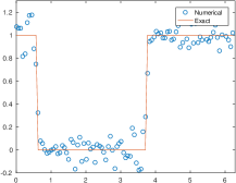
(a) without any limiter

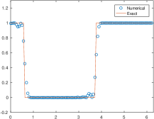
(b) with only the bound-preserving limiter

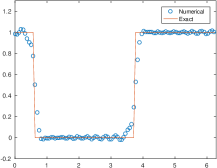
(c) with only the TVB limiter

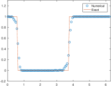
(d) with both limiters

Figure 1: Linear convection at $T=10$. Fourth order compact finite difference and fourth order SSP multistep with $\Delta t=\frac{1}{3}C_{ms}\Delta x$ and $100$ grid points. The TVB parameter in (11) is $p=5$.

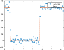
(a) Without any limiter.

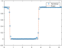
(b) With the bound-preserving limiter.

Figure 2: Linear convection at $T=10$. Eighth order compact finite difference and the fourth order SSP multistep method with $\Delta t=C_{ms}\frac{6}{25}\Delta x$ and $100$ grid points

Example 2.

One dimensional Burgers’ equation.

Consider the Burgers’ equation $u_{t}+(\frac{u^{2}}{2})_{x}=0$ with a periodic boundary condition on $[-\pi,\pi]$. For the initial data $u_{0}(x)=\sin(x)+0.5$, the exact solution is smooth up to $T=1$, then it develops a moving shock. We list the errors of the fourth order scheme at $T=0.5$ in Table 3 where the time step is $\Delta t=\frac{1}{3}C_{ms}\Delta x$ for SSP multistep and $\Delta t=\frac{5}{3}C_{ms}\Delta x$ for SSP Runge-Kutta with $\Delta x=\frac{2\pi}{N}$. We observe the expected fourth order accuracy for the multistep time discretization. At $T=1.2$, the exact solution contains a shock near $x=-2.5$. The errors on the smooth region $[-2,\pi]$ at $T=1.2$ are listed in Table 4 where high order accuracy is lost. Some high order schemes can still be high order accurate on a smooth region away from the shock in this test, see [22]. We emphasize that in all our numerical tests, Step III in Algorithm 2 was never triggered. In other words, set of Class I is rarely encountered in practice. So the limiter Algorithm 2 is a local three-point stencil limiter for this particular example rather than a global one. The loss of accuracy in smooth regions is possibly due to the fact that compact finite difference operator is defined globally thus the error near discontinuities will pollute the whole domain.

The solutions of the fourth order compact finite difference and the fourth order SSP multistep with the bound-preserving limiter and the TVB limiter at time $T=2$ are shown in Figure 3, for which the exact solution is in the range $[-0.5,1.5]$. The TVB limiter alone does not eliminate the overshoot or undershoot. When both the bound-preserving and the TVB limiters are used, we can obtain a non-oscillatory bound-preserving numerical solution.

Table 3: The fourth order scheme with limiter for the Burgers’ equation. Smooth solutions.

	Fourth order SSP multistep				Fourth SSP Runge-Kutta
N	$L^{1}$ error	order	$L^{\infty}$ error	order	$L^{1}$ error	order	$L^{\infty}$ error	order
$20$	6.92E-4	-	5.24E-3	-	7.79E-4	-	5.61E-3	-
$40$	3.28E-5	4.40	3.62E-4	3.85	4.45E-5	4.13	4.77E-4	3.56
$80$	1.90E-6	4.11	2.00E-5	4.18	3.53E-6	3.66	2.09E-5	4.51
$160$	1.15E-6	4.04	1.24E-6	4.01	4.93E-7	2.84	5.47E-6	1.93
$320$	7.18E-9	4.00	7.67E-8	4.01	8.78E-8	2.49	1.73E-6	1.66

Table 4: Burgers’ equation. The errors are measured in the smooth region away from the shock.

	Fourth order SSP multistep				Fourth SSP Runge-Kutta
N	$L^{1}$ error	order	$L^{\infty}$ error	order	$L^{1}$ error	order	$L^{\infty}$ error	order
$20$	1.59E-2	-	5.26E-2	-	1.62E-2	-	5.39E-2	-
$40$	2.10E-3	2.92	1.38E-2	1.93	2.11E-3	2.94	1.39E-2	1.95
$80$	6.35E-4	1.73	6.56E-3	1.07	6.48E-4	1.70	7.01E-3	0.99
$160$	1.48E-4	2.10	1.65E-3	1.99	1.51E-4	2.10	1.66E-3	2.08
$320$	3.12E-5	2.25	6.10E-4	1.43	3.14E-5	2.26	6.13E-4	1.44

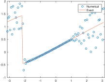
(a) without any limiter

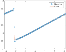
(b) with both limiters

Figure 3: Burgers’ equation at $T=2$. Fourth order compact finite difference with $\Delta t=\frac{1}{3\max_{x}|u_{0}(x)|}C_{ms}\Delta x$ and $100$ grid points. The TVB parameter in (11) is set as $p=5$.

Example 3.

One dimensional convection diffusion equation.

Consider the linear convection diffusion equation $u_{t}+cu_{x}=du_{xx}$ with a periodic boundary condition on $[0,2\pi]$. For the initial $u_{0}(x)=\sin(x)$, the exact solution is $u(x,t)=exp(-dt)sin(x-ct)$ which is in the range $[-1,1]$. We set $c=1$ and $d=0.001$. The errors of the fourth order scheme at $T=1$ are listed in the Table 5 in which $\Delta t=C_{ms}min\{\frac{1}{6}\frac{\Delta x}{c},\frac{5}{24}\frac{\Delta x^{2}}{d}\}$ for SSP multistep and $\Delta t=5C_{ms}min\{\frac{1}{6}\frac{\Delta x}{c},\frac{5}{24}\frac{\Delta x^{2}}{d}\}$ for SSP Runge-Kutta with $\Delta x=\frac{2\pi}{N}$. We observe the expected fourth order accuracy for the SSP multistep method. Even though the bound-preserving limiter is triggered, the order reduction for the Runge-Kutta method is not observed for the convection diffusion equation. One possible explanation is that the source of such an order reduction is due to the lower order accuracy of inner stages in the Runge-Kutta method, which is proportional to the time step. Compared to $\Delta t=\mathcal{O}(\Delta x)$ for a pure convection, the time step is $\Delta t=\mathcal{O}(\Delta x^{2})$ in a convection diffusion problem thus the order reduction is much less prominent. See the Table 6 for the errors at $T=1$ of the eighth order scheme with $\Delta t=C_{ms}\min\{\frac{3}{25}\frac{\Delta x^{2}}{c},\frac{131}{530}\frac{\Delta x^{2}}{d}\}$ for SSP multistep and $\Delta t=5C_{ms}\min\{\frac{3}{25}\frac{\Delta x^{2}}{c},\frac{131}{530}\frac{\Delta x^{2}}{d}\}$ for SSP Runge-Kutta where $\Delta x=\frac{2\pi}{N}$.

Table 5: The fourth order compact finite difference with limiter for linear convection diffusion.

	Fourth order SSP multistep				Fourth order SSP Runge-Kutta
N	$L^{1}$ error	order	$L^{\infty}$ error	order	$L^{1}$ error	order	$L^{\infty}$ error	order
$20$	3.30E-5	-	5.19E-5	-	3.60E-5	-	6.09E-5	-
$40$	2.11E-6	3.97	3.30E-6	3.97	2.44E-6	4.00	3.52E-6	4.12
$80$	1.33E-7	3.99	2.09E-7	3.98	1.37E-7	4.04	2.15E-7	4.03
$160$	8.36E-9	3.99	1.31E-8	3.99	8.46E-9	4.02	1.33E-8	4.02
$320$	5.24E-10	4.00	8.23E-10	4.00	5.29E-10	4.00	8.31E-10	4.00

Table 6: The eighth order compact finite difference with limiter for linear convection diffusion.

	SSP multistep				SSP Runge-Kutta
N	$L^{1}$ error	order	$L^{\infty}$ error	order	$L^{1}$ error	order	$L^{\infty}$ error	order
$10$	3.85E-7	-	5.96E-7	-	3.85E-7	-	5.95E-7	-
$20$	1.40E-9	8.10	2.20E-9	8.08	1.42E-9	8.08	2.23E-9	8.06
$40$	5.46E-12	8.01	8.60E-12	8.00	5.48E-12	8.02	8.69E-12	8.01
$80$	3.53E-12	0.63	6.46E-12	0.41	1.06E-12	2.37	3.29E-12	1.40

Example 4.

Nonlinear degenerate diffusion equations.

A representative test for validating the positivity-preserving property of a scheme solving nonlinear diffusion equations is the porous medium equation, $u_{t}=(u^{m})_{xx},m>1.$ We consider the Barenblatt analytical solution given by

$$B_{m}(x,t)=t^{-k}[(1-\frac{k(m-1)}{2m}\frac{|x|^{2}}{t^{2k}})_{+}]^{1/(m-1)},$$

where $u_{+}=\max\{u,0\}$ and $k=(m+1)^{-1}$. The initial data is the Barenblatt solution at $T=1$ with periodic boundary conditions on $\left[-6,6\right]$. The solution is computed till time $T=2$. High order schemes without any particular positivity treatment will generate negative solutions [21, 26, 14]. See Figure 4 for solutions of the fourth order scheme and the SSP multistep method with $\Delta t=\frac{1}{3m}C_{ms}\Delta x$ and $100$ grid points. Numerical solutions are strictly nonnegative. Without the bound-preserving limiter, negative values emerge near the sharp gradients.

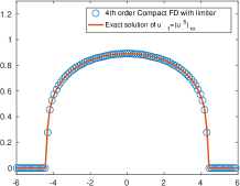
(a) $m=5.$

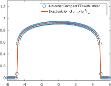
(b) $m=8.$

Figure 4: The fourth order compact finite difference with limiter for the porous medium equation.

6.2 One-dimensional problems with non-periodic boundary conditions

Example 5.

One-dimensional Burgers’ equation with inflow-outflow boundary condition. Consider $u_{t}+(\frac{u^{2}}{2})_{x}=0$ on interval $[0,2\pi]$ with inflow-outflow boundary condition and smooth initial condition $u(x,0)=u_{0}(x)$. Let $u_{0}(x)=\frac{1}{2}\sin(x)+\frac{1}{2}\geq 0$, we can set the left boundary condition as inflow $u(0,t)=L(t)$ and right boundary as outflow, where $L(t)$ is obtained from the exact solution of initial-boundary value problem for the same initial data and a periodic boundary condition. We test the fourth order compact finite difference and fourth order SSP multistep method with the bound-preserving limiter. The errors at $T=0.5$ are listed in Table 7 where $\Delta t=C_{ms}\Delta x$ and $\Delta x=\frac{2\pi}{N}$. See Figure 5 for the shock at $T=3$ on a $120$-point grid with $\Delta t=C_{ms}\Delta x$.

Table 7: Burgers’ equation. The fourth order scheme. Inflow and outflow boundary conditions.

N	$L^{\infty}$ error	order	$L^{1}$ error	order
$20$	1.15E-4	-	7.80E-4	-
$40$	4.10E-6	4.81	2.00E-5	5.29
$80$	2.17E-7	4.24	9.43E-7	4.40
$160$	1.22E-8	4.15	4.87E-8	4.28
$320$	7.41E-10	4.05	2.87E-9	4.09

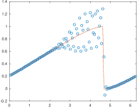
(a) Without any limiter.

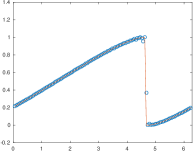
(b) With the bound-preserving limiter.

Figure 5: Burgers’ equation. The fourth order scheme. Inflow and outflow boundary conditions.

Example 6.

One-dimensional convection diffusion equation with Dirichlet boundary conditions. We consider equation $u_{t}+cu_{x}=du_{xx}$ on $[0,2\pi]$ with boundary conditions $u(0,t)=\cos(-ct)e^{-dt}$ and $u(2\pi,t)=\cos(2\pi-ct)e^{-dt}$. The exact solution is $u(x,y,t)=\cos(x-ct)e^{-dt}$. We set $c=1$ and $d=0.01$. We test the third order boundary scheme proposed in Section 5.2 and the fourth order interior compact finite difference with the fourth order SSP multistep time discretization. The errors at $T=1$ are listed in Table 8 where $\Delta t=C_{ms}\min\{\frac{4}{19}\frac{\Delta x}{c},\frac{695}{1596}\frac{\Delta x^{2}}{d}\}$, $\Delta x=\frac{2\pi}{N}$.

Table 8: A linear convection diffusion equation with Dirichlet boundary conditions.

N	$L^{\infty}$ error	order	$L^{1}$ error	order
$10$	1.68E-3	-	8.76E-3	-
$20$	1.47E-4	3.51	7.12E-4	3.62
$40$	8.35E-6	4.14	4.27E-5	4.06
$80$	4.44E-7	4.23	2.28E-6	4.23
$160$	2.30E-8	4.27	1.10E-7	4.37

6.3 Two-dimensional problems with periodic boundary conditions

In this subsection we test the fourth order compact finite difference scheme solving two-dimensional problems with periodic boundary conditions.

Example 7.

Two-dimensional linear convection equation. Consider $u_{t}+u_{x}+u_{y}=0$ on the domain $[0,2\pi]\times[0,2\pi]$ with a periodic boundary condition. The scheme is tested with a smooth initial condition $u_{0}(x,y)=\frac{1}{2}+\frac{1}{2}\sin^{4}(x+y)$ to verify the accuracy. The errors at time $T=1$ are listed in Table 9 where $\Delta t=C_{ms}\frac{1}{6}\Delta x$ for the SSP multistep method and $\Delta t=5C_{ms}\frac{1}{6}\Delta x$ for the SSP Runge-Kutta method with $\Delta x=\Delta y=\frac{2\pi}{N}$. We can observe the fourth order accuracy for the multistep method on resolved meshes and obvious order reductions for the Runge-Kutta method.

Table 9: Fourth order accurate compact finite difference with limiter for the 2D linear equation.

	Fourth order SSP multistep				Fourth order SSP Runge-Kutta
$N\times N$ Mesh	$L^{1}$ error	order	$L^{\infty}$ error	order	$L^{1}$ error	order	$L^{\infty}$ error	order
$10\times 10$	4.70E-2	-	1.17E-1	-	8.45E-2	-	1.07E-1	-
$20\times 20$	5.47E-3	3.10	8.97E-3	3.71	5.56E-3	3.93	9.09E-3	3.56
$40\times 40$	3.04E-4	4.17	5.09E-4	4.13	2.88E-4	4.27	6.13E-4	3.89
$80\times 80$	1.78E-5	4.09	2.99E-5	4.09	1.95E-5	3.89	6.77E-5	3.18
$160\times 160$	1.09E-6	4.03	1.85E-6	4.01	2.65E-6	2.88	1.26E-5	2.43

We also test the following discontinuous initial data:

$$u_{0}(x,y)=\left\{\begin{array}[]{ll}1,&\textrm{if $(x,y)\in[-0.2,0.2]\times[-0.2,0.2]$},\\ 0,&\textrm{otherwise}.\end{array}\right.$$

The numerical solutions on a $80\times 80$ mesh at $T=0.5$ are shown in Figure 6 with $\Delta t=\frac{1}{6}C_{ms}\Delta x$ and $\Delta x=\Delta y=\frac{2\pi}{N}$. Fourth order SSP multistep method is used.

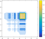
(a) Without any limiter.

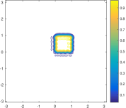
(b) With bound-preserving limiter.

Figure 6: Fourth order compact finite difference for the 2D linear convection.

Example 8.

Two-dimensional Burgers’ equation. Consider $u_{t}+(\frac{u^{2}}{2})_{x}+(\frac{u^{2}}{2})_{y}=0$ with $u_{0}(x,y)=0.5+\sin(x+y)$ and periodic boundary conditions on $[-\pi,\pi]\times[-\pi,\pi]$. At time $T=0.2$, the solution is smooth and the errors at $T=0.2$ on a $N\times N$ mesh are shown in the Table 10 in which $\Delta t=C_{ms}\frac{\Delta x}{6\max_{x}|u_{0}(x)|}$ for multistep and $\Delta t=5C_{ms}\frac{\Delta x}{6\max_{x}|u_{0}(x)|}$ for Runge-Kutta with $\Delta x=\Delta y=\frac{2\pi}{N}$. At time $T=1$, the exact solution contains a shock. The numerical solutions of the fourth order SSP multistep method on a $100\times 100$ mesh are shown in Figure 7 where $\Delta t=\frac{1}{6\max_{x}|u_{0}(x)|}C_{ms}\Delta x$. The bound-preserving limiter ensures the solution to be in the range $[-0.5,1.5]$.

Table 10: Fourth order compact finite difference scheme with the bound-preserving limiter for the 2D Burgers’ equation.

	SSP multistep				SSP Runge-Kutta
$N\times N$ Mesh	$L^{1}$ error	order	$L^{\infty}$ error	order	$L^{1}$ error	order	$L^{\infty}$ error	order
$10\times 10$	1.08E-2	-	4.48E-3	-	9.16E-3	-	3.73E-2	-
$20\times 20$	4.73E-4	4.52	3.76E-3	3.58	2.90E-4	4.98	2.14E-3	4.12
$40\times 40$	1.90E-5	4.64	1.45E-4	4.69	2.03E-5	3.83	1.12E-4	4.25
$80\times 80$	9.99E-7	4.25	7.43E-6	4.29	2.35E-6	3.12	1.54E-5	2.86
$160\times 160$	5.87E-8	4.09	4.26E-7	4.13	3.62E-7	2.70	5.13E-6	1.59

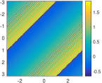
(a) Without the bound-preserving limiter

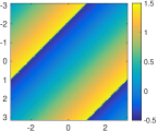
(b) With the bound-preserving limiter

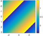
(c) The exact solution

Figure 7: The fourth order scheme. 2D Burgers’ equation.

Example 9.

Two-dimensional convection diffusion equation.

Consider the equation $u_{t}+c(u_{x}+u_{y})=d(u_{xx}+u_{yy})$ with $u_{0}(x,y)=\sin(x+y)$ and a periodic boundary condition on $[0,2\pi]\times[0,2\pi]$. The errors at time $T=0.5$ for $c=1$ and $d=0.001$ are listed in Table 11, in which $\Delta t=C_{ms}\min\{\frac{\Delta x}{6c},\frac{5\Delta x^{2}}{48d}\}$ for the fourth-order SSP multistep method, and $\Delta t=5C_{ms}\min\{\frac{\Delta x}{6c},\frac{5\Delta x^{2}}{48d}\}$ for the fourth-order SSP Runge-Kutta method, where $\Delta x=\Delta y=\frac{2\pi}{N}$.

Table 11: Fourth order compact finite difference with limiter for the 2D convection diffusion equation.

	Fourth order SSP multistep				Fourth order SSP Runge-Kutta
N	$L^{1}$ error	order	$L^{\infty}$ error	order	$L^{1}$ error	order	$L^{\infty}$ error	order
$10\times 10$	6.26E-4	-	9.67E-4	-	6.68E-4	-	9.59E-4	-
$20\times 20$	3.62E-5	4.11	5.61E-5	4.11	3.60E-5	4.21	6.09E-5	3.98
$40\times 40$	2.20E-6	4.04	3.45E-6	4.02	2.24E-6	4.00	3.52E-6	4.12
$80\times 80$	1.35E-7	4.02	2.13E-7	4.01	1.37E-7	4.04	2.15E-7	4.03
$160\times 160$	8.45E-9	4.01	1.33E-8	4.01	8.46E-9	4.02	1.33E-8	4.02

Example 10.

Two-dimensional porous medium equation.

We consider the equation $u_{t}=\Delta(u^{m})$ with the following initial data

$$u_{0}(x,y)=\left\{\begin{array}[]{ll}1,&\textrm{if $(x,y)\in[-0.5,0.5]\times[-0.5,0.5]$,}\\ 0,&\textrm{if $(x,y)\in[-2,2]\times[-2,2]/[-1,1]\times[-1,1]$,}\end{array}\right.$$

and a periodic boundary condition on domain $[-2,2]\times[-2,2]$. See Figure 8 for the solutions at time $T=0.01$ for SSP multistep method with $\Delta t=\frac{5}{48\max_{x}|u_{0}(x)|}C_{ms}\Delta x$ and $\Delta x=\Delta y=\frac{1}{15}$. The numerical solutions are strictly non-negative, which is nontrivial for high order accurate schemes. High order schemes without any positivity treatment will generate negative solutions in this test, see [21, 26, 14].

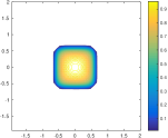
(a) $m=3$.

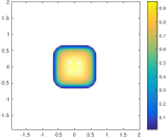
(b) $m=4$.

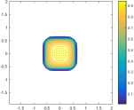
(c) $m=5$.

Figure 8: The fourth order scheme with limiter for 2D porous medium equations $u_{t}=\Delta(u^{m})$.

7 Concluding remarks

In this paper we have demonstrated that fourth order accurate compact finite difference schemes for convection diffusion problems with periodic boundary conditions satisfy a weak monotonicity property, and a simple three-point stencil limiter can enforce bounds without destroying the global conservation. Since the limiter is designed based on an intrinsic property in the high order finite difference schemes, the accuracy of the limiter can be easily justified. This is the first time that the weak monotonicity is established for a high order accurate finite difference scheme, complementary to results regarding the weak monotonicity property of high order finite volume and discontinuous Galerkin schemes in [23, 24, 25].

We have discussed extensions to two dimensions, higher order accurate schemes and general boundary conditions, for which the five-diagonal weighting matrices can be factored as a product of tridiagonal matrices so that the same simple three-point stencil bound-preserving limiter can still be used. We have also proved that the TVB limiter in [3] does not affect the bound-preserving property. Thus with both the TVB and the bound-preserving limiters, the numerical solutions of high order compact finite difference scheme can be rendered non-oscillatory and strictly bound-preserving without losing accuracy and global conservation. Numerical results suggest the good performance of the high order bound-preserving compact finite difference schemes.

For more generalizations and applications, there are certain complications. For using compact finite difference schemes on non-uniform meshes, one popular approach is to introduce a mapping to a uniform grid but such a mapping results in an extra variable coefficient which may affect the weak monotonicity. Thus any extension to non-uniform grids is much less straightforward. For applications to systems, e.g., preserving positivity of density and pressure in compressible Euler equations, the weak monotonicity can be easily extended to a weak positivity property. However, the same three-point stencil limiter cannot enforce the positivity for pressure. One has to construct a new limiter for systems.

References

• [1] Mark H Carpenter, David Gottlieb, and Saul Abarbanel, The stability of numerical boundary treatments for compact high-order finite-difference schemes, Journal of Computational Physics 108 (1993), no. 2, 272–295.
• [2] Zheng Chen, Hongying Huang, and Jue Yan, Third order maximum-principle-satisfying direct discontinuous Galerkin methods for time dependent convection diffusion equations on unstructured triangular meshes, Journal of Computational Physics 308 (2016), 198–217.
• [3] Bernardo Cockburn and Chi-Wang Shu, Nonlinearly stable compact schemes for shock calculations, SIAM Journal on Numerical Analysis 31 (1994), no. 3, 607–627.
• [4] Sigal Gottlieb, David I Ketcheson, and Chi-Wang Shu, Strong stability preserving Runge-Kutta and multistep time discretizations, World Scientific, 2011.
• [5] Jingwei Hu, Ruiwen Shu, and Xiangxiong Zhang, Asymptotic-preserving and positivity-preserving implicit-explicit schemes for the stiff bgk equation, SIAM Journal on Numerical Analysis 56 (2018), no. 2, 942–973.
• [6] Sanjiva K Lele, Compact finite difference schemes with spectral-like resolution, Journal of computational physics 103 (1992), no. 1, 16–42.
• [7] Randall J LeVeque, Numerical methods for conservation laws, Birkhauser Basel, 1992.
• [8] Doron Levy and Eitan Tadmor, Non-oscillatory central schemes for the incompressible 2-D Euler equations, Mathematical Research Letters 4 (1997), 321–340.
• [9] Xu-Dong Liu and Stanley Osher, Nonoscillatory high order accurate self-similar maximum principle satisfying shock capturing schemes I, SIAM Journal on Numerical Analysis 33 (1996), no. 2, 760–779.
• [10] Yuan Liu, Yingda Cheng, and Chi-Wang Shu, A simple bound-preserving sweeping technique for conservative numerical approximations, Journal of Scientific Computing 73 (2017), no. 2-3, 1028–1071.
• [11] Tong Qin and Chi-Wang Shu, Implicit positivity-preserving high-order discontinuous galerkin methods for conservation laws, SIAM Journal on Scientific Computing 40 (2018), no. 1, A81–A107.
• [12] Richard Sanders, A third-order accurate variation nonexpansive difference scheme for single nonlinear conservation laws, Mathematics of Computation 51 (1988), no. 184, 535–558.
• [13] WF Spotz and GF Carey, High-order compact finite difference methods, Preliminary Proceedings International Conference on Spectral and High Order Methods, Houston, TX, 1995, pp. 397–408.
• [14] Sashank Srinivasan, Jonathan Poggie, and Xiangxiong Zhang, A positivity-preserving high order discontinuous galerkin scheme for convection–diffusion equations, Journal of Computational Physics 366 (2018), 120–143.
• [15] Zheng Sun, José A Carrillo, and Chi-Wang Shu, A discontinuous Galerkin method for nonlinear parabolic equations and gradient flow problems with interaction potentials, Journal of Computational Physics 352 (2018), 76–104.
• [16] Andrei I Tolstykh, High accuracy non-centered compact difference schemes for fluid dynamics applications, vol. 21, World Scientific, 1994.
• [17] Andrei I Tolstykh and Michael V Lipavskii, On performance of methods with third-and fifth-order compact upwind differencing, Journal of Computational Physics 140 (1998), no. 2, 205–232.
• [18] Tao Xiong, Jing-Mei Qiu, and Zhengfu Xu, High order maximum-principle-preserving discontinuous Galerkin method for convection-diffusion equations, SIAM Journal on Scientific Computing 37 (2015), no. 2, A583–A608.
• [19] Zhengfu Xu, Parametrized maximum principle preserving flux limiters for high order schemes solving hyperbolic conservation laws: one-dimensional scalar problem, Mathematics of Computation 83 (2014), no. 289, 2213–2238.
• [20] Xiangxiong Zhang, On positivity-preserving high order discontinuous galerkin schemes for compressible navier–stokes equations, Journal of Computational Physics 328 (2017), 301–343.
• [21] Xiangxiong Zhang, Yuanyuan Liu, and Chi-Wang Shu, Maximum-principle-satisfying high order finite volume weighted essentially nonoscillatory schemes for convection-diffusion equations, SIAM Journal on Scientific Computing 34 (2012), no. 2, A627–A658.
• [22] Xiangxiong Zhang and Chi-Wang Shu, A genuinely high order total variation diminishing scheme for one-dimensional scalar conservation laws, SIAM Journal on Numerical Analysis 48 (2010), no. 2, 772–795.
• [23]  , On maximum-principle-satisfying high order schemes for scalar conservation laws, Journal of Computational Physics 229 (2010), no. 9, 3091–3120.
• [24]  , Maximum-principle-satisfying and positivity-preserving high-order schemes for conservation laws: survey and new developments, Proceedings of the Royal Society of London A: Mathematical, Physical and Engineering Sciences, vol. 467, The Royal Society, 2011, pp. 2752–2776.
• [25] Xiangxiong Zhang, Yinhua Xia, and Chi-Wang Shu, Maximum-principle-satisfying and positivity-preserving high order discontinuous Galerkin schemes for conservation laws on triangular meshes, Journal of Scientific Computing 50 (2012), no. 1, 29–62.
• [26] Yifan Zhang, Xiangxiong Zhang, and Chi-Wang Shu, Maximum-principle-satisfying second order discontinuous Galerkin schemes for convection–diffusion equations on triangular meshes, Journal of Computational Physics 234 (2013), 295–316.