Physicality of evolution and statistical contractivity are equivalent notions of maps

Abstract

Statistical quantifiers are generically required to contract under physical evolutions, following the intuition that information should be lost under noisy transformations. This principle is very relevant in statistics, and it even allows to derive uniqueness results based on it: by imposing their contractivity under any physical maps, the Chentsov-Petz theorem singles out a unique family of metrics on the space of probability distributions (or density matrices) called the Fisher information metrics. This result might suggest that statistical quantifiers are a derived concept, as their very definition is based on physical maps. The aim of this work is to disprove this belief. Indeed, we present a result dual to the Chentsov-Petz theorem, proving that among all possible linear maps, the only ones that contract the Fisher information are exactly the physical ones. This result shows that, contrary to the common opinion, there is no fundamental hierarchy between physical maps and canonical statistical quantifiers, as either of them can be defined in terms of the other.

I Introduction

The result that gave birth to information theory, Shannon’s noiseless coding theorem, answers the question of what is the maximum rate at which a message can be transmitted over an ideal transmission line Shannon (1948); Holevo (2013). This can be phrased in terms of the relative entropy, defined for two discrete probability vectors $\bm{p}$ and $\bm{q}$ as:

$$D(\bm{p}||\bm{q}):=\sum_{i}\;p_{i}\,\log\frac{p_{i}}{q_{i}}\,,$$ (1)

where $p_{i}/q_{i}$ are the components of the two vectors. Then, the minimum compression is connected to the statistical difference, as measured by $D(\bm{p}||\bm{q})$, between the code probability distribution and the uniform one. Thanks to the operational interpretation of the relative entropy as the asymptotic difference between the two log-likelihood Kullback (1997), this result simply means that in order for a probabilistic code to work, it needs to generate correlations significantly different from random bits.

Over time, information theory evolved from its role in telecommunication to become one of the cornerstones of the modern understanding of physics. Indeed, apart from its decisive role in the treatment of statistical mechanics Jaynes (1957); Leff and Rex (2014); Parrondo et al. (2015), its extension to the quantum regime gave rise to an entire new field of physics Nielsen and Chuang (2002). Today, the concept of information plays a foundational role very similar to the one of energy for classical mechanics. For example, we impose time-reversal symmetry by requiring that the global evolution of a closed system conserves the information, singling out in this way unitaries and antiunitaries transformations, in agreement with Wigner’s theorem Holevo (2013). Moreover, much in the same way in which one reconciles the existence of dissipative dynamics with the principle of conservation of energy, we explain the existence of evolutions for which information appears to be lost by postulating that the missing information is simply transferred to some environmental degrees of freedom which we do not have access to. Following this argument, the most generic quantum mechanical evolution $\Phi$ takes the form:

$$\Phi(\rho_{S})=\mathrm{Tr}_{E}\left[U_{SE}\,(\rho_{S}\otimes\omega_{E})\,U_{SE}^{\dagger}\right]\,,$$ (2)

where $\rho_{S}$ is the state of the system, $\omega_{E}$ is a generic environmental state and $U_{SE}$ is the global unitary/antiunitary evolution. Moreover, requiring the compatibility with composition of different systems, further restricts the set of global transformations $U_{SE}$ to unitaries only Życzkowski and Bengtsson (2004); Chiribella et al. (2021). The class of maps defined by Eq. (2), with $U_{SE}$ restricted to be unitary, is characterised by Stinespring theorem Stinespring (1955) as the set of Completely Positive Trace-Preserving maps (CPTP). When the same reasoning is applied to classical probabilities, one obtains the set of stochastic maps, since these can always be decomposed as:

$$[T(\bm{p})]_{i}=\sum_{j,k,l}U_{ij}^{kl}p_{k}\omega_{l}\;,$$ (3)

where $\bm{p}$ represents the classical probability distribution of the system, $\bm{\omega}$ the one of the environment, while $U$ is a global isometry.

Despite their different origins, statistical quantifiers and dynamical maps are deeply connected. For one thing, the relative entropy in Eq. (1) (as well as its quantum counterpart $H_{L}(\rho||\sigma):=\mathrm{Tr}\left[\rho(\log\rho-\log\sigma)\right]$) contracts under physical evolutions:

$$D(\bm{p}||\bm{q})\geq D(T(\bm{p})||T(\bm{q}))\,,$$ (4)

for any stochastic transformation $T$. Similarly, any sensible generalisation of the relative entropy needs to satisfy a condition akin to Eq. (4), corresponding to the intuition that information cannot increase during noisy transformations. This connection becomes even more compelling when one looks at the local behaviour of statistical quantifiers: a renown theorem by Chentsov establishes that there exists a unique metric on the space of classical probability distributions that is contractive under any stochastic (i.e., physical) map Chentsov (2000); Campbell (1986). This takes the name of Fisher information metric, or Fisher-Rao metric, and it is given by $\eta_{i,j}\big{|}_{\bm{p}}:=\frac{\delta_{i,j}}{p_{i}}$. In this way, dynamical considerations constrain the local behaviour of any possible statistical quantifier. The deep connection between dynamics and Fisher information Abiuso et al. (2023); Scandi et al. (2023) has been mostly overlooked in the literature, as more operative uses were explored Cramer (1946); Rao (1992); Ly et al. (2017).

Still, there is another path to the Fisher metric that we want to highlight here. In an effort to gather the many possible statistical quantifiers present in the literature, Csiszár introduced the concept of $f$-divergences, a continuous family generalising many of the main properties of the relative entropy Csiszár and Shields (2004). Interestingly though, despite the wide range of possible definitions, it was noticed that for close-by probabilities (in the sense that $\bm{q}=\bm{p}+{\rm d}\bm{q}$ for some $||{\rm d}\bm{q}||\ll 1$) all the $f$-divergences reduce to the Fisher information. Indeed, if we take for example the relative entropy in Eq. (1) it is a matter of Taylor-expanding the logarithm to see that:

$$D(\bm{p}||\bm{p}+{\rm d}\bm{q})\simeq\sum_{i}\;\frac{{\rm d}q_{i}^{2}}{p_{i}}=\sum_{i,j}\;{\rm d}q_{i}\,\eta_{i,j}\big{|}_{\bm{p}}\,{\rm d}q_{j}\,,$$ (5)

up to higher order corrections in ${\rm d}\bm{q}$. This shows that the Fisher information metric could also be defined in purely statistical terms, that is, independently of any dynamical considerations.

Indeed, even if one might think that there is a hierarchy between physical maps and Fisher information (and, therefore, statistical quantifiers), in which the latter derives from the first, we show in this work that the situation is actually more intertwined: we prove that physical evolutions can be defined solely in terms of the Fisher information metric. Before doing this, though, we need to introduce the concept of contrast functions and Fisher information metrics for quantum states.

II Quantum Fisher Information metrics

In this section we give a brief overview of the quantum Fisher information metrics, presenting in particular its statistical derivation (Thm. 1) and the dynamical one (Thm. 2). Given the technicality of the subject we will only outline the main definitions, and we refer the reader to the review in Scandi et al. (2023) for further details.

Let us then introduce the concept of contrast functions $H(\rho||\sigma)$ between two quantum states $\rho$ and $\sigma$. This notion was first introduced for classical statistics by Csiszár Csiszár and Shields (2004), and later extended by Petz to the quantum regime Petz (1986), following an effort to give an axiomatic foundation to the many different divergences present in the literature. In particular, the principles proposed are the following:

1. positivity: meaning that $H(\rho||\sigma)\geq 0$, with equality iff $\rho\equiv\sigma$. As contrast functions should assess the statistical difference between two states, they should be non-negative (and detect when two states are the same);

2. joint convexity: this is specified mathematically as ${H(\lambda\rho_{1}+(1-\lambda)\rho_{2}||\lambda\sigma_{1}+(1-\lambda)\sigma_{2})\;\leq}\allowbreak{\lambda H(\rho_{1}||\sigma_{1})+(1-\lambda)H(\rho_{2}||\sigma_{2})}$, for $0\leq\lambda\leq 1$, corresponding to the intuition that mixing states should not increase their information content;

3. monotonicity: that is $H(\Phi(\rho)||\Phi(\sigma))\leq H(\rho||\sigma)$ for any CPTP map $\Phi$. As it was mentioned in the introduction, this condition ensures the compatibility with physical evolutions;

4. differentiability: meaning that the function $h_{\rho,\sigma}(x,y):=H(\rho+xA||\sigma+yB)$, for $A$ and $B$ any Hermitian operators, is $C^{\infty}$. This is a regularity condition, required when interested in the local Riemannian behaviour of $H$.

These conditions are still not enough to single out a unique family of statistical quantifiers, and for this reason it is customary to also propose an ansatz, which encompasses most of the examples defined in the literature. In particular, the one proposed in Petz (1986) reads as follows:

$$H_{g}(\rho||\sigma):=\mathrm{Tr}\left[g\bm{(}\mathbb{L}_{\sigma}\mathbb{R}_{\rho}^{-1}\bm{)}\left[\rho\right]\right]\,,$$ (6)

where $g:\mathbb{R}^{+}\rightarrow\mathbb{R}$ is a matrix convex function Hiai and Petz (2014), and $\mathbb{L}_{\rho}$ and $\mathbb{R}_{\rho}$ are the left and right multiplication operators, acting as:

$$\mathbb{L}_{\rho}[A]=\rho\,A\,,\qquad\qquad\mathbb{R}_{\rho}[A]=A\,\rho\,.$$ (7)

It should be noticed that despite being a very large family, containing the relative entropy (when $g(x)=-\log x$), and functionals related to the Rényi divergences, the definition in Eq. (6) is still not enough to completely exhaust all the possibilities present in the literature Scandi et al. (2023). Still, it is enough to define the entire family of Fisher information metrics. Indeed, we have the following:

Theorem 1 (Lesniewski, Ruskai Lesniewski and Ruskai (1999)).

The contrast functions $H_{g}(\pi+\varepsilon A||\pi+\varepsilon B)$ can be locally approximated up to corrections of order $\mathcal{O}\left(\varepsilon^{3}\right)$ as:

$$H_{g}(\pi+\varepsilon A||\pi+\varepsilon B)\simeq\frac{\varepsilon^{2}}{2}\,\mathrm{Tr}\left[(A-B)\,\mathbb{J}_{f}^{-1}\big{|}_{\pi}[(A-B)]\right]\,,$$ (8)

where $A$ and $B$ are traceless, Hermitian perturbations, and the superoperator $\mathbb{J}_{f}\big{|}_{\pi}$, called the quantum Fisher operator, is defined as:

$$\mathbb{J}_{f}\big{|}_{\pi}:=\mathbb{R}_{\pi}\,f\bm{(}\mathbb{L}_{\pi}\mathbb{R}_{\pi}^{-1}\bm{)}\,.$$ (9)

Moreover, $f$ is an operator monotone function connected to $g$ by the equation:

$$f(x)=\frac{(x-1)^{2}}{g(x)+x\,g(x^{-1})}\,.$$ (10)

This represents the first possible derivation of the Fisher information metrics for quantum systems. Still, in order to claim that the operators in Eq. (9) define all and only the Fisher information metrics we need to resort to their dynamical characterisation, i.e., their contractivity under arbitrary CPTP maps. This is provided by the independent result of Petz:

Theorem 2 (Petz Petz (1996)).

All the metrics on quantum states that contract under arbitrary CPTP maps are of the form:

$$K_{f,\pi}(A,B):=\mathrm{Tr}\left[A\,\,\mathbb{J}_{f}^{-1}\big{|}_{\pi}[B]\right],$$ (11)

where $f:\mathbb{R}^{+}\rightarrow\mathbb{R}^{+}$ is an operator monotone function from the family in Eq. (10).

This result makes the definition of Fisher information metrics in the quantum regime unambiguous. Indeed, even if the single metric $\eta_{i,j}\big{|}_{\bm{p}}$ is now replaced by a continuous family of possible operators $\mathbb{J}^{-1}_{f}\big{|}_{\pi}$, each one describing the local behaviour of a different contrast function (Thm. 1), it would not be correct to postulate some extra axioms to isolate a unique quantity. Indeed, Thm. 2 tells us that narrowing down the family in Eq. (9) would also destroy the connection with the dynamical characterisation of the Fisher information metrics.

III Contractivity implies physicality

In this section we prove our main result, that is how the property of statistical contractivity isolates physical evolutions among all possible linear maps. Our main mathematical theorem (Thm. 3) characterizes positive maps via their contraction of the Fisher information metric. This can be then extended to complete positivity (Cor. 3.1) and contrast functions contractivity (Cor. 3.2).

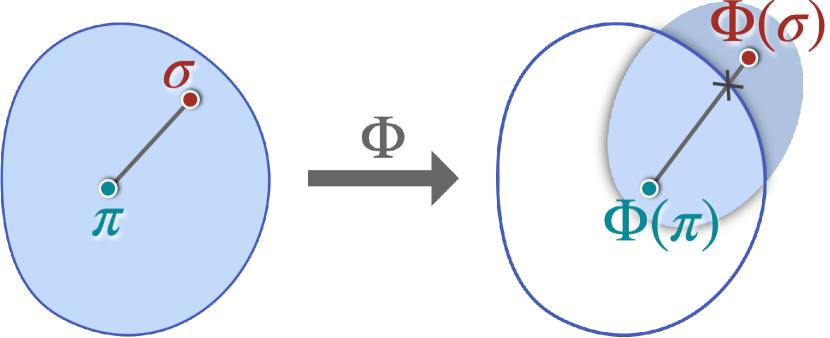
Figure 1: Sketch of the proof of Thm. 3: thanks to condition 1 one can always find a point $\pi$ in $\mathcal{P}^{\circ}_{d}$ that gets mapped into $\mathcal{P}^{\circ}_{d}$. Now assume there is a matrix $\sigma$ in the $\mathcal{P}^{\circ}_{d}$ that gets mapped outside of $\mathcal{P}_{d}$. Then, the segment connecting $\pi$ to $\sigma$ will be mapped into a curve intersecting the boundary of $\mathcal{P}_{d}$. Since the Fisher information is bounded on the interior of the space of states, and diverges on its boundary, there must be a point for which the Fisher metric increases.

Define $\mathcal{M}_{d}(\mathbb{C})$ to be the space of $d\times d$ complex matrices, $\mathcal{P}_{d}\subset\mathcal{M}_{d}(\mathbb{C})$ to be the subset of positive semidefinite matrices, and $\mathcal{S}_{d}\subset\mathcal{P}_{d}$ the space of states, i.e., the matrices in $\mathcal{P}_{d}$ with trace one. Moreover, denote the interior of a set $X$ as $X^{\circ}$. Then, it holds that:

Theorem 3.

Consider a Hermitian preserving, linear map $\Phi:\mathcal{M}_{d}(\mathbb{C})\rightarrow\mathcal{M}_{d}(\mathbb{C})$. If $\Phi$ satisfies the following two properties:

1. $\Phi$ maps at least one point from $\mathcal{P}^{\circ}_{d}$ into $\mathcal{P}^{\circ}_{d}$;

2. for any matrix $\rho\in\mathcal{P}^{\circ}_{d}$ such that $\Phi(\rho)\in\mathcal{P}^{\circ}_{d}$, and any vector $\delta\rho$ in the $\mathcal{P}_{d}$-tangent space, one has:

   $$K_{f,\rho}(\delta\rho,\delta\rho)\geq K_{f,\Phi(\rho)}(\Phi(\delta\rho),\Phi(\delta\rho))\,;$$ (12)

then the image of ${\Phi}$ is completely contained in $\mathcal{P}_{d}$, meaning that $\Phi$ is a positive map (P). Moreover, $\Phi$ is trace non-increasing.

We refer the reader to Appendix 1 for the precise proof of the theorem. The main idea is explained in Fig. 1, and it leverages the fact that the Fisher information metric is bounded in the interior of $\mathcal{P}_{d}$, while it diverges on its boundary. Then, one can prove the claim by contradiction: if there is even a single point in $\mathcal{P}_{d}^{\circ}$ that gets mapped outside of $\mathcal{P}_{d}$, thanks to the linearity of $\Phi$, one can define a segment in $\mathcal{P}_{d}^{\circ}$ whose image will intersect the boundary of $\mathcal{P}_{d}$ (see Fig. 1). This allows to find a point for which the Fisher metric expands, contradicting condition 2 and proving the claim.

There are a couple of remarks to be made: first, it should be noticed that since the Fisher information metrics are only defined on $\mathcal{P}_{d}^{\circ}$, condition 1 is minimal to introduce the concept of contractivity (encoded by Eq. (12)). Moreover, the restriction on the set of $\rho$ considered at the beginning of condition 2 is also minimal in order for the two sides of Eq. (12) to be regular, i.e., we only focus on matrices $\rho$ for which both the Fisher metrics in $\rho$ and in $\Phi(\rho)$ are well-defined. Finally, let us notice that the use of $\mathcal{P}_{d}$ as a domain was chosen to show the mathematical result in full generality, as well as to accommodate potentially trace non-preserving maps. In this sense, the theorem again isolates physical maps, which can only decrease the probability-normalization of states . In the corollaries that follows we restrict, for clarity, to standard trace-preserving (TP) maps on the physical set of states $\mathcal{S}_{d}$.

Corollary 3.1.

Consider a Hermitian preserving, trace-preserving linear map $\Phi:\mathcal{M}_{d}(\mathbb{C})\rightarrow\mathcal{M}_{d}(\mathbb{C})$. If $\Phi$ satisfies the following two properties:

1. it maps at least one point from $\mathcal{S}^{\circ}_{d}$ into $\mathcal{S}^{\circ}_{d}$;

2. for all $\rho\in\mathcal{S}^{\circ}_{d}$ such that $\Phi(\rho)\in\mathcal{S}^{\circ}_{d}$, and for all $\delta\rho$ in the $\mathcal{S}_{d}$-tangent space, it contracts the Fisher metric as in Eq. (12);

Then $\Phi$ is a positive map (PTP). Moreover, if $\Phi\otimes\mathds{I}_{d}$, acting on $(\mathcal{S}_{d}\otimes\mathcal{S}_{d})^{\circ}$, satisfies the same conditions, then $\Phi$ is a completely positive map (CPTP).

The proof of the corollary is contained at the end of Appendix 1, and it is equivalent to the one for Thm. 3. It should be noticed that Thm. 3 and Cor. 3.1 completely characterize physical evolutions: the first gives a condition for positivity, which is sufficient for classical systems, while the latter characterise CPTP maps, the relevant notion of maps for quantum systems.

We conclude by observing that the same results can be phrased in terms of any of the contrast functions introduced above. In fact, putting together Thm. 1 with Cor. 3.1, we have:

Corollary 3.2.

Consider a Hermitian preserving, trace preserving, linear map $\Phi:\mathcal{M}_{d}(\mathbb{C})\rightarrow\mathcal{M}_{d}(\mathbb{C})$ mapping at least one point from $\mathcal{S}^{\circ}_{d}$ into $\mathcal{S}^{\circ}_{d}$. Consider any contrast function $H_{g}(\rho||\sigma)$. If for every two states $\rho$ and $\sigma$ in $\mathcal{S}_{d}^{o}$ it holds that:

$$H_{g}(\rho||\sigma)\geq H_{g}(\Phi(\rho)||\Phi(\sigma))\,,$$ (13)

then $\Phi$ is a positive map (PTP). Moreover, if the same holds for $\Phi\otimes\mathds{I}_{d}$ then the map is completely positive (CPTP).

We refer to Appendix 2 for the precise proof, but this result simply follows from the fact that all contrast functions locally expand to Fisher metrics, hence it is sufficient to choose $\rho$ and $\sigma$ to be close-by matrices and then apply Thm. 3 to them. Cor. 3.2 shows that it is enough to consider any divergence to actually characterise the class of positive (or completely positive) maps. In fact, while our results are more general, a specific instance of Cor. 3.2 can be expressed as follows:

If a linear map acting on the set of states (including, in the quantum case, ancillas with trivial dynamics) can only reduce their relative entropy, then such map represents a physical evolution.

IV Conclusion

In the axiomatic definition of quantum statistical divergences, the monotonicity condition 3 stands out as the only request which is not purely statistical in nature: indeed, whereas the other properties can be expressed solely in terms of states, in order to introduce monotonicity one needs to explicitly introduce the concept of noisy transformations. This fact might suggest that there is some hierarchy between physical evolutions and statistical quantifiers, since one needs the first to define the latter. Corroborating this belief, the Chentsov-Petz theorem (Thm. 2) constrains the local behaviour of statistical distances, singling out the Fisher information through a purely dynamical request.

Still, historically most of the contrast functions were introduced in a purely statistical setting, therefore their strong connection with dynamics is a priori not obvious and, indeed, quite remarkable. This manuscript, then, aims at clarifying this fortunate conjunction: Thm. 3 and its Cor. 3.1 show that physical evolutions can be singled out as the unique family of linear maps that contract the Fisher information. This result not only justifies the claim that physicality of evolution and statistical contractivity are equivalent notions of maps, but also hints at the source of this connection, as both dynamical maps and statistical distances arise from the underlying notion of conservation of information.

Moreover, Cor. 3.2 also shows how one could in principle define physical evolutions merely in terms of any contrast function, strengthening the message that there is no intrinsic hierarchy of fundamentality between statistical notions and dynamical ones. Still, it should be kept in mind that Thm. 2 is peculiar to the Fisher information, further corroborating the natural role this quantity plays both in quantum and classical physics.

In fact, it was noticed that many dynamical aspects of evolutions, as Markovianity or detailed balance, can be naturally phrased in terms of the behaviour of maps with respect to the Fisher metrics Abiuso et al. (2023); Scandi et al. (2023). The results presented here suggest that this is far from being a coincidence, showing that there is a fundamental connection which is worth exploring further in future works. Moreover, in the context of the reconstructions of quantum mechanics Hardy (2015); Mueller and Masanes (2015), the fact that physical evolutions can be singled out in terms of a statistical quantity as the Fisher information might be of particular relevance for the derivation of a sensible notion of dynamics.

V Acknowledgements

M.S. acknowledges the support of project Intramural 20235AT009 of the Spanish National Research Council. P.A. is supported by the QuantERA II programme, that has received funding from the European Union’s Horizon 2020 research and innovation programme under Grant Agreement No 101017733, and from the Austrian Science Fund (FWF), project I-6004. Research at the Perimeter Institute for Theoretical Physics is supported by the Government of Canada through the Department of Innovation, Science and Economic Development Canada and by the Province of Ontario through the Ministry of Research, Innovation and Science. D.D.S. is supported by the research project “Dynamics and Information Research Institute - Quantum Information, Quantum Technologies” within the agreement between UniCredit Bank and Scuola Normale Superiore di Pisa (CI14_UNICREDIT_MARMI).

Appendix A Methods

Appendix B 1. Proof of Thm. 3 and Cor. 3.1

In this appendix we present the proof of Thm. 3, which we repeat here for convenience:

Theorem.

Consider a Hermitian preserving, linear map $\Phi:\mathcal{M}_{d}(\mathbb{C})\rightarrow\mathcal{M}_{d}(\mathbb{C})$. If $\Phi$ satisfies the following two properties:

1. $\Phi$ maps at least one point from $\mathcal{P}^{\circ}_{d}$ into $\mathcal{P}^{\circ}_{d}$;

2. for any matrix $\rho$ in $\mathcal{P}^{\circ}_{d}\cap\bm{(}\Phi^{-1}\bm{(}\mathcal{P}^{\circ}_{d}\cap\Phi(\mathcal{P}_{d})\bm{)}\bm{)}$, and any tangent vector $\delta\rho$, one has:

   $$K_{f,\rho}(\delta\rho,\delta\rho)\geq K_{f,\Phi(\rho)}(\Phi(\delta\rho),\Phi(\delta\rho))\,;$$ (14)

then the image of ${\Phi}$ is completely contained in $\mathcal{P}_{d}$, meaning that $\Phi$ is a positive map (P). Moreover, $\Phi$ is trace non-increasing.

Proof.

We prove Theorem 3 by contradiction: suppose there exists a map $\Phi$ that is not positive, but that satisfies Eq. (14). Thanks to condition 1 there exists at least one point $\pi$ in $\mathcal{P}^{\circ}_{d}$ such that its evolution is also in the interior of $\mathcal{P}_{d}$. Moreover, from the assumption that $\Phi$ is not P there is also at least one matrix $\sigma$ such that ${\Phi}(\sigma)\notin\mathcal{P}_{d}$. Without loss of generality one can choose $\sigma$ to be in the interior of $\mathcal{P}_{d}$: if this is not the case we take a ball around $\sigma$ small enough so that its image still lays outside of the state space. Then, by inspecting the intersection between the preimage of this ball and $\mathcal{P}^{\circ}_{d}$ one can find a point satisfying the assumption. Since both $\rho$ and $\sigma$ are in $\mathcal{P}^{\circ}_{d}$, the line $\rho_{\lambda}:=(1-\lambda)\,\pi+\lambda\,\sigma$ is completely contained in $\mathcal{P}^{\circ}_{d}$ for $\lambda\in[0,1]$. This implies that the following superior is finite:

$$\sup_{\lambda,\mathrm{Tr}\left[\delta\rho^{2}\right]=1} \,K_{f,\rho_{\lambda}}(\delta\rho,\delta\rho)=\sup_{\lambda,\mathrm{Tr}\left[\delta\rho^{2}\right]=1}\,\mathrm{Tr}\left[\delta\rho\,\mathbb{J}_{f}^{-1}\big{|}_{\rho_{\lambda}}[\delta\rho]\right]<\infty\,,$$ (15)

since the Fisher information is a bounded operator when restricted to a closed set completely inside of $\mathcal{P}_{d}^{\circ}$ (see Scandi et al. (2023)). By varying $\lambda$, ${\Phi}(\rho_{\lambda})$ interpolates linearly between the positive definite matrix ${\Phi}(\pi)$ and one with at least one negative eigenvalue, namely ${\Phi}(\sigma)$. Then, there exists a $\lambda^{*}$ such that ${\Phi}(\rho_{\lambda^{*}})$ is a matrix with at least one zero-eigenvalue. We are now ready to prove the claim. Set the state $\rho_{\eta}$ so that the smallest eigenvalue $\epsilon_{\eta}$ of ${\Phi}(\rho_{\eta})$ is of order $\eta$, where $\eta\ll 1$. Call the associated eigenvector $\ket{\psi_{\eta}}$. Then, choose a perturbation $\delta\rho_{\eta}$ such that, for any $\eta$, $\Phi(\delta\rho_{\eta})$ has a positive and finite contribution along the eigenvectors corresponding to $\eta$-eigenvalues (the positivity condition ensures that in the limit $\eta\rightarrow 0$ the perturbed state is still in the interior of $\mathcal{P}^{\circ}_{d}$ for any finite $\eta$, allowing for the definition of the Fisher information). One can always find such a perturbation. Suppose, in fact, the contrary. Then, this would mean that for any $\delta\rho$, it holds that:

$$\lim_{\eta\rightarrow 0}\bra{\psi_{\eta}}\Phi(\delta\rho)\ket{\psi_{\eta}}=0\quad\forall\,\delta\rho.$$ (16)

But any $\delta\rho$ can always be rewritten as $\delta\rho=\sigma_{1}-\sigma_{2}$, where $\sigma_{1/2}\in\mathcal{P}_{d}$. Then, Eq. (16) would imply that for any two matrices in $\mathcal{P}_{d}$ it holds that:

$$\bra{\psi_{0}}\Phi(\sigma_{1})\ket{\psi_{0}}=\bra{\psi_{0}}\Phi(\sigma_{2})\ket{\psi_{0}}\quad\forall\sigma_{1},\sigma_{2}\in\mathcal{P}_{d}\;.$$ (17)

Set $\sigma_{2}:=\rho_{\lambda^{*}}$, which, by definition, satisfies $\bra{\psi_{0}}\Phi(\rho_{\lambda^{*}})\ket{\psi_{0}}=0$. This implies that for any matrix in $\sigma\in\mathcal{P}_{d}$, the image of $\sigma$ is not full-rank, since $\bra{\psi_{0}}\Phi(\sigma)\ket{\psi_{0}}=0$, which in turns contradicts the hypothesis that at least one point in $\mathcal{P}^{\circ}_{d}$ is mapped inside $\mathcal{P}^{\circ}_{d}$. Thus, there exists at least one $\delta\rho_{\eta}$ for which Eq. (16) does not hold. Then, choosing such a vector, one can see that the evolved Fisher information is unbounded as $\eta\rightarrow 0$ by explicit inspection of its coordinates expression:

$$K_{f,{\Phi}(\rho_{\eta})}(\Phi(\delta\rho_{\eta}),\Phi(\delta\rho_{\eta}))=\sum_{i\neq j}\;\frac{|\Phi(\delta\rho_{\eta})_{ij}|^{2}}{\Phi(\rho_{\eta})_{jj}f\bm{(}\Phi(\rho_{\eta})_{ii}/\Phi(\rho_{\eta})_{jj}\bm{)}}+\sum_{i}\frac{|\Phi(\delta\rho_{\eta})_{ii}|^{2}}{\Phi(\rho_{\eta})_{ii}}$$ (18)

where we used the formula for the Fisher information in the orthonormal basis of $\Phi(\rho_{\eta})$ provided in Scandi et al. (2023). All the terms in the two sums are positive. Moreover, the second sum diverges at least as $\mathcal{O}\left(\eta^{-1}\right)$ as $\eta\rightarrow 0$, due to the contribution associated to the eigenvalue of $\ket{\psi_{\eta}}$. Hence, we can always find a $\eta$ small enough such that:

$$K_{f,{\Phi}(\rho_{\eta})}({\Phi}(\delta\rho_{\eta}),{\Phi}(\delta\rho_{\eta}))>\sup_{\lambda,\mathrm{Tr}\left[\delta\rho^{2}\right]=1}\,K_{f,\rho_{\lambda}}(\delta\rho,\delta\rho)\geq K_{f,\rho_{\eta}}(\delta\rho_{\eta},\delta\rho_{\eta})\;,$$ (19)

contradicting the assumption that ${\Phi}$ contracts the Fisher metric for any two points in $\mathcal{P}_{d}^{\circ}$. This proves the Positivity of $\Phi$. Moreover, choosing $\delta\rho\equiv\rho$ in Eq. (14), one obtains:

$$\mathrm{Tr}\left[\rho\right]=K_{f,\rho}(\delta\rho,\delta\rho)\geq K_{f,\Phi(\rho)}(\Phi(\delta\rho),\Phi(\delta\rho))=\mathrm{Tr}\left[\Phi(\rho)\right]\,,$$ (20)

thanks to the property that $\mathbb{J}_{f}^{-1}\big{|}_{\rho}[\rho]=\mathds{I}$ Scandi et al. (2023). This proves that $\Phi$ is trace non-increasing. ∎

Finally, regarding Cor. 3.1, it should be noticed that the only difference is that the tangent space of $\mathcal{S}_{d}$ is given by traceless Hermitian operators. Thus, whereas tangent vectors to $\mathcal{P}_{d}$ can be written as $\delta\rho=\sigma_{1}-\sigma_{2}$ for $\sigma_{1/2}\in\mathcal{P}_{d}$, in the case of $\mathcal{S}_{d}$ the same decomposition still holds, but with $\sigma_{1/2}\in\mathcal{S}_{d}$. Then, one can prove the existence of the perturbation $\delta\rho_{\eta}$ in the very same way as we did for $\mathcal{P}_{d}$.

Appendix C 2. Proof of Corollary 3.2

We prove Corollary 3.2, which we repeat here for convenience:

Corollary.

Consider a Hermitian preserving, linear map $\Phi:\mathcal{M}_{d}(\mathbb{C})\rightarrow\mathcal{M}_{d}(\mathbb{C})$ satisfying condition 1 in Thm. 3. Consider any contrast function $H_{g}(\rho||\sigma)$. If for every two matrices $\rho$ and $\sigma$ on $\mathcal{P}_{d}^{o}$ it holds that:

$$H_{g}(\rho||\sigma)\geq H_{g}(\Phi(\rho)||\Phi(\sigma))\,,$$ (21)

then $\Phi$ is a positive map. Moreover, if the same holds for $\Phi\otimes\mathds{I}_{d}$ then the map is completely positive.

Proof.

The proof of the corollary directly follows from the one of Thm. 3. Indeed, by contradiction, assume there exists a matrix $\sigma\in\mathcal{P}^{\circ}_{d}$ that gets mapped outside of $\mathcal{P}_{d}$, and consider $\pi\in\mathcal{P}^{\circ}_{d}$ such that $\Phi(\pi)\in\mathcal{P}^{\circ}_{d}$. Analogously to the proof above, define $\rho_{\lambda}:=(1-\lambda)\,\pi+\lambda\,\sigma$. For $\varepsilon$ small enough we can apply Thm. 1 to obtain:

$$\sup_{\lambda,\mathrm{Tr}\left[\delta\rho^{2}\right]=1}\,H_{g}(\rho_{\lambda}||\rho_{\lambda}+\varepsilon\,\delta\rho)=\sup_{\lambda,\mathrm{Tr}\left[\delta\rho^{2}\right]=1}\,\frac{\varepsilon^{2}}{2}\,K_{f,\rho_{\lambda}}(\delta\rho,\delta\rho)+\mathcal{O}\left(\varepsilon^{3}\right)<\infty\,.$$ (22)

Then, following the steps presented for Thm. 3, we define a $\rho_{\eta}$ such that $\Phi(\rho_{\eta})$ is of order $\eta$, where $\eta\ll 1$, and a $\delta\rho_{\eta}$ having a positive finite contribution along the eigenvectors corresponding to $\eta$-eigenvalues. The positivity condition ensures that in the limit $\eta\rightarrow 0$ the perturbed state is still in the interior of $\mathcal{P}_{d}$ for any finite $\eta$, and $\varepsilon$ small enough. Then, $H_{g}(\Phi(\rho_{\eta})||\Phi(\rho_{\eta}+\varepsilon\,\delta\rho_{\eta}))$ scales as $\varepsilon^{2}/\eta$. Hence, one can find $\eta$ small enough such that:

$$H_{g}(\Phi(\rho_{\eta})||\Phi(\rho_{\eta}+\varepsilon\,\delta\rho_{\eta}))>\sup_{\lambda,\mathrm{Tr}\left[\delta\rho^{2}\right]=1}\,H_{g}(\rho_{\lambda}||\rho_{\lambda}+\varepsilon\,\delta\rho)\geq\;H_{g}(\rho_{\eta}||\rho_{\eta}+\varepsilon\,\delta\rho_{\eta})\,.$$ (23)

This gives the desired contradiction, concluding the proof. ∎

References

- Shannon (1948) C. E. Shannon, “A mathematical theory of communication,” The Bell System Technical Journal 27, 379–423 (1948).
- Holevo (2013) A. S. Holevo, Quantum Systems, Channels, Information. A Mathematical Introduction. (De Gruyter, Berlin, Boston, 2013).
- Kullback (1997) S. Kullback, Information Theory and Statistics, Dover Books on Mathematics (Dover Publications, Mineola, NY, 1997).
- Jaynes (1957) E. T. Jaynes, “Information theory and statistical mechanics,” Phys. Rev. 106, 620–630 (1957).
- Leff and Rex (2014) H. S. Leff and A. F. Rex, Maxwell’s Demon: Entropy, Information, Computing, Princeton Series in Physics (Princeton University Press, 2014).
- Parrondo et al. (2015) J. M. R. Parrondo, J. M. Horowitz, and T. Sagawa, “Thermodynamics of information,” Nature Physics 11, 131–139 (2015).
- Nielsen and Chuang (2002) M. A. Nielsen and I. Chuang, Quantum computation and quantum information (American Association of Physics Teachers, 2002).
- Życzkowski and Bengtsson (2004) K. Życzkowski and I. Bengtsson, “On duality between quantum maps and quantum states,” Open systems & information dynamics 11, 3–42 (2004).
- Chiribella et al. (2021) G. Chiribella, E. Aurell, and K. Życzkowski, “Symmetries of quantum evolutions,” Physical Review Research 3, 033028 (2021).
- Stinespring (1955) W. F. Stinespring, “Positive functions on C∗ -algebras,” Proceedings of the American Mathematical Society 6, 211 (1955).
- Chentsov (2000) N. N. Chentsov, Statistical decision rules and optimal inference (American Mathematical Soc., 2000).
- Campbell (1986) L. L. Campbell, “An extended Čencov characterization of the information metric,” Proceedings of the American Mathematical Society 98, 135–141 (1986).
- Abiuso et al. (2023) Paolo Abiuso, Matteo Scandi, Dario De Santis, and Jacopo Surace, “Characterizing (non-)Markovianity through Fisher information,” SciPost Phys. 15, 014 (2023).
- Scandi et al. (2023) M. Scandi, P. Abiuso, J. Surace, and D. De Santis, “Quantum Fisher information and its dynamical nature,” arXiv preprint arXiv:2304.14984 (2023).
- Cramer (1946) H. Cramer, Mathematical methods of statistics (Princeton University Press, 1946).
- Rao (1992) C. R. Rao, “Information and the accuracy attainable in the estimation of statistical parameters,” Kotz S., Johnson N.L. (eds) Breakthroughs in Statistics. Springer Series in Statistics (Perspectives in Statistics) (1992), 10.1007/978-1-4612-0919-5.
- Ly et al. (2017) A. Ly, M. Marsman, J. Verhagen, R. P. P. P. Grasman, and E.-J. Wagenmakers, “A Tutorial on Fisher information,” Journal of Mathematical Psychology 80, 40–55 (2017).
- Csiszár and Shields (2004) I. Csiszár and P. C. Shields, Information theory and statistics: a tutorial, Vol. 1 (Now Publishers, Inc., 2004) pp. 417–528.
- Petz (1986) D. Petz, “Quasi-entropies for finite quantum systems,” Reports on Mathematical Physics 23, 57–65 (1986).
- Hiai and Petz (2014) F. Hiai and D. Petz, Introduction to matrix analysis and applications, Universitext (Springer, 2014).
- Lesniewski and Ruskai (1999) A. Lesniewski and M. B. Ruskai, “Monotone Riemannian metrics and relative entropy on non-commutative probability spaces,” Journal of Mathematical Physics 40, 5702–5724 (1999).
- Petz (1996) D. Petz, “Monotone metrics on matrix spaces,” Linear Algebra and its Applications 244, 81–96 (1996).
- Note (1) Maps that decrease the trace correspond to evolutions with post-selection, i.e., with a non-null probability of discarding the system.
- Hardy (2015) L. Hardy, “Reconstructing quantum theory,” in Quantum theory: informational foundations and foils (Springer, 2015) pp. 223–248.
- Mueller and Masanes (2015) M. P. Mueller and L. Masanes, “Information-theoretic postulates for quantum theory,” in Quantum theory: informational foundations and foils (Springer, 2015) pp. 139–170.