Graph Deep Learning for Time Series Forecasting

Abstract

Graph-based deep learning methods have become popular tools to process collections of correlated time series. Differently from traditional multivariate forecasting methods, neural graph-based predictors take advantage of pairwise relationships by conditioning forecasts on a (possibly dynamic) graph spanning the time series collection. The conditioning can take the form of an architectural inductive bias on the neural forecasting architecture, resulting in a family of deep learning models called spatiotemporal graph neural networks. Such relational inductive biases enable the training of global forecasting models on large time-series collections, while at the same time localizing predictions w.r.t. each element in the set (i.e., graph nodes) by accounting for local correlations among them (i.e., graph edges). Indeed, recent theoretical and practical advances in graph neural networks and deep learning for time series forecasting make the adoption of such processing frameworks appealing and timely. However, most of the studies in the literature focus on proposing variations of existing neural architectures by taking advantage of modern deep learning practices, while foundational and methodological aspects have not been subject to systematic investigations. To fill the gap, this paper aims to introduce a comprehensive methodological framework that formalizes the forecasting problem and provides design principles for graph-based predictive models and methods to assess their performance. At the same time, together with an overview of the field, we provide design guidelines, recommendations, and best practices, as well as an in-depth discussion of open challenges and future research directions.

1 Introduction

Shallow and deep neural architectures have been used to forecast time series for decades resulting in stories of both failure [177] and success [150, 93]. One of the key elements enabling most of the recent achievements in the field is the training of a single global neural network – with shared parameters – on large collections of related time series [140, 12]. Indeed, training a single global model allows for scaling the complexity of the architecture given the larger available sample size. Such an approach, however, considers each time series independently from the others and, as a consequence, does not take into account dependencies that might be instrumental for accurate predictions [59]. For example, the large variety of sensors that permeates modern cyber-physical infrastructures (e.g., traffic networks and smart grids) produces sets of time series with inherently rich spatiotemporal structure and spatiotemporal dynamics. On one hand, global models appear inadequate in capturing such dependencies across time series, while, on the other, training a single local predictor, i.e., modeling the full collection as a large multivariate time series, would negate the benefits brought by sharing the trainable parameters. Furthermore, both approaches would not allow for exploiting any prior information, such as the directionality and sparsity of the dependencies.

The way out, as it often happens with major advancements in both deep learning [94, 69, 142] and time series forecasting [68, 45], is to consider the structure of the data as an inductive bias. Indeed, the dependency structure of the data can be represented in terms of pairwise relationships between the time series in the collection. The resulting representation is a graph where each time series is associated with a node and functional dependencies among them are represented as edges. The conditioning of the predictor on observations at correlated time series can then take the form of an architectural inductive bias in the processing carried out by the neural architecture. Graph neural networks (GNNs) [6, 18], based on the message-passing (MP) framework [58], provide the suitable neural operators allowing for sharing parameters in the processing of the time series, while, at the same time, conditioning the predictions w.r.t. observations at neighboring nodes (related time series). The resulting models, operating over both time and space, are known as spatiotemporal graph neural networks (STGNNs) [144, 98, 37, 82]. STGNNs implement global and inductive architectures for time series processing by exploiting the MP mechanisms to account for spatial – other than temporal – dynamics, with the term spatial referring to dynamics that span the collection across different time series.

Researchers have been proposing a large variety of STGNNs by integrating MP into popular architectures, e.g., by exploiting MP blocks to implement the gates of recurrent cells [144, 98, 34, 115] and to propagate representations in fully convolutional [168, 161] and attention-based architectures [181, 163, 113]. The adoption of the resulting STGNNs has been successful in a wide range of time series processing applications ranging from traffic flow prediction [98, 168, 161] and air quality monitoring [25, 75] to energy analytics [48, 36], financial time series processing [28, 114] and epidemiological data analysis [83, 53]. However, despite the rich literature on architectures and successful applications, the methodological foundations of the field have not been systematically laid out yet. For instance, the categorization of STGNNs as global models and the interplay between globality and locality have been studied in such context only recently [37], regardless of the profound practical implications. We argue that a comprehensive formalization and methodological framework for the design of graph-based deep learning methods in time series forecasting is missing. The goal of this paper is, hence, to frame the problem from the proper perspective and propose a framework instrumental to tackling the inherent challenges of the field, ranging from learning the latent graph underlying the observed data to dealing with local effects, missing data, and scalability issues.

Our contributions can be summarised as follows. We

• provide a formalization of the problem settings (Sec. 3) and of the time series forecasting problem given relational side information and the inductive bias associated with the proposed graph-based framework (Sec. 4);

• present guidelines to design effective graph-based forecasting architectures (Sec. 5–7) and to evaluate their performance (Sec. 8);

• identify the challenges inherent to such problem settings and discuss the associated design choices (Sec. 10) addressing, in particular, the problem of dealing with missing data (Sec. 10.1), latent graph learning (Sec. 10.2), the scalability of the resulting models (Sec. 10.3) and learning in inductive settings (Sec. 10.4).

Simulation results (Sec. 9), a discussion of the related works (Sec. 2) and future directions (Sec. 11) complete the paper. We believe that the introduced comprehensive design framework will aid researchers in investigating the foundational aspects of graph deep learning for time series processing and, at the same time, provide practitioners with both the practical and theoretical guidelines needed to apply such methods to real-world problems.

2 Related works

Graph deep learning methods have found widespread application in the processing of temporal data [84, 171, 63, 108, 82]. In this section, we review previous related works that investigate different sub-areas within the field.

Dynamic relational data

The term temporal graph (or temporal network) is used to indicate scenarios where nodes, attributes, and edges of a graph are dynamic and are given over time as a sequence of events localized at specific nodes and/or as the interactions among them [84, 108]. A typical reference application is the processing of the dynamic relationships and user profiles that characterize social networks and recommender systems. Kazemi et al. [84] propose an encoder-decoder framework to unify existing representation learning methods for dynamic graphs. Barros et al. [9] compiled a rich survey of methods for embedding dynamic networks, while Skarding et al. [149] focus on GNN approaches to the same problem. Longa et al. [108] introduce a taxonomy of tasks and models in temporal graph processing; Gravina and Bacciu [63], along with a categorization of existing architectures, introduce a benchmark based on a diverse set of available datasets. Huang et al. [72] build an alternative set of benchmarks and datasets with a focus on applications to large-scale temporal graphs. Besides temporal graphs, a large body of literature has been dedicated to the processing of sequences of arbitrary graphs, e.g., without assuming any correspondence between nodes across time steps [171, 174]. Although the settings we deal with in this paper could formally be seen as a sub-area of temporal graph processing, having actual time series associated with each node radically changes the approach to the problem, as well as the available model designs and target applications. Indeed, none of the above-mentioned frameworks explicitly target time series forecasting.

Graph-based time series processing

Spatiotemporal graph neural networks for time series processing have been pioneered in the context of traffic forecasting [98, 168] and the application of graph deep learning methods in traffic analytics have been extremely successful [164, 79, 80]. The analysis of STGNNs in the context of global and local forecasting models has been initiated in [37]. Jin et al. [82] carried out an in-depth survey of GNNs architectures for time series forecasting, classification, imputation, and anomaly detection. In contrast, the present paper does not focus on surveying architectures but on providing a foundational methodological framework together with guidelines for the practitioner. More similarly in spirit to our work, Benidis et al. [12] provide a tutorial and a critical discussion of modern practices in deep learning for time series forecasting. Analogously, Bronstein et al. [18] and Bacciu et al. [6] provide frameworks for understanding and developing graph deep learning methods. Finally, outside of deep learning, graph-based methods for time series processing have been studied in the context of graph signal processing [124, 151, 95] and go under the name of time-vertex signal processing methods [60].

3 Problem settings

This section formalizes the problem settings. In particular, Sec. 3.1 introduces the reference framework, suitably extended in Sec. 3.2 to deal with specific scenarios typical of various application domains.

3.1 Reference problem settings

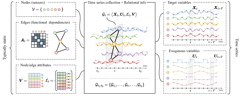
Figure 1: A collection of synchronous and regularly sampled time series with associated pairwise dependencies.

We consider collections of correlated time series with side relational information.

Correlated time series

Consider a collection of $N$, regularly and synchronously sampled, correlated time series; the $i$-th time series is composed by a sequence of $d_{x}$-dimensional vectors ${\bm{x}}^{i}_{t}\in{\mathbb{R}}^{d_{x}}$ observed at each time step $t$ and coming from sensors with $d_{x}$ channels each. Time series are assumed to be homogenous, i.e., characterized by the same variables (observables) – say the same $d_{x}$ channels. Matrix ${\bm{X}}_{t}\in{\mathbb{R}}^{N\times d_{x}}$ denotes the stacked $N$ observations at time $t$, while ${\bm{X}}_{t:t+T}$ indicates the sequence of observations within time interval $[t,t+T)$; with the shorthand ${\bm{X}}_{<t}$ we indicate observations at time steps up to $t$ (excluded). Exogenous variables associated with each time series are denoted by ${\bm{U}}_{t}\in{\mathbb{R}}^{N\times d_{u}}$, while static (time-independent) attributes are grouped in matrix ${\bm{V}}\in{\mathbb{R}}^{N\times d_{v}}$. We consider a setup where observations have been generated by a time-invariant spatiotemporal stochastic process such that

$${\bm{x}}_{t}^{i}\sim p^{i}\left({\bm{x}}_{t}^{i}\big{|}{\bm{X}}_{<t},{\bm{U}}_{\leq t},{\bm{V}}\right)\quad\forall i=1,\dots,N;$$ (1)

in particular, we assume the existence of a predictive causality à la Granger [59], i.e., we assume that forecasts for a single time series can benefit – in terms of accuracy – from accounting for the past values of (a subset of) other time series in the collection. Each time series $\{{\bm{x}}_{t}^{i}\}_{t}$ might indeed be generated by a different stochastic process, i.e., in general, $p^{i}\neq p^{j}$ if $i\neq j$. In the sequel, the term spatial refers to the dimension of size $N$, that spans the time series collection; in the case of physical sensors, the term spatial reflects the fact that each time series might correspond to a different physical location.

Relational information

Relational dependencies among the time series collection can be exploited to inform the downstream processing and allow for, e.g., getting rid of spurious correlations in the observed sequences of data. Pairwise relationships existing among the time series can be encoded by a (possibly dynamic) adjacency matrix ${\bm{A}}_{t}\in\{0,1\}^{N\times N}$ that accounts for the (possibly asymmetric) dependencies at time step $t$; optional edge attributes ${\bm{e}}^{ij}_{t}\in{\mathbb{R}}^{d_{e}}$ can be associated to each non-zero entry of ${\bm{A}}_{t}$. In particular, we denote the set of attributed edges encoding all the available relational information by ${{\mathcal{E}}_{t}\doteq\{\langle(i,j),{\bm{e}}^{ij}_{t}\rangle\ |\ \forall i,j:{\bm{A}}_{t}[i,j]\neq 0\}}$. Whenever edge attributes are scalar, i.e., $d_{e}=1$, edge set ${\mathcal{E}}_{t}$ can be simply represented as a weighted and real-valued adjacency matrix ${\bm{A}}_{t}\in{\mathbb{R}}^{N\times N}$. Analogously to the homogeneity assumption for observations, edges are assumed to indicate the same type of relational dependencies (e.g., physical proximity) and have the same type of attributes across the collection. We use interchangeably the terms node and sensor to indicate each of the $N$ entities generating the time series and refer to the node set together with the relational information as sensor network. The tuple ${\mathcal{G}}_{t}\doteq\langle{\bm{X}}_{t},{\bm{U}}_{t},{\mathcal{E}}_{t},{\bm{V}}\rangle$ indicates all the available information at time step $t$. Finally, note that for many applications (e.g., traffic networks) changes in the topology happen slowly over time and the adjacency matrix – as well as edge attributes – can be considered as fixed within a short window of observations, i.e., ${\mathcal{E}}_{t}={\mathcal{E}}$ and ${\bm{e}}^{ij}_{t}={\bm{e}}^{ij}$ for all $(i,j)$ pairs. A graphical representation of the problem settings is shown in Fig. 1.

Example 1.

Consider a sensor network monitoring the speed of vehicles at crossroads. In this case, ${\bm{X}}_{1:t}$ refers to past traffic speed measurements sampled at a certain frequency. Exogenous variables ${\bm{U}}_{t}$ account for time-of-the-day and day-of-the-week identifiers, and the current weather conditions. The node-attribute matrix ${\bm{V}}$ collects static features related to the sensor’s position, e.g., the type of road the sensor is placed in or the number of lanes. A static adjacency matrix ${\bm{A}}$ can be obtained by considering each pair of sensors connected by an edge – weighted by the road distance – if and only if a road segment directly connects them. Conversely, road closures and traffic diversions can be accounted for by adopting a dynamic topology ${\bm{A}}_{t}$.

3.2 Extensions to the reference settings

This section offers extensions to the reference problem settings by discussing how the framework can be modified to account for peculiarities typical of a wide range of practical applications.

New nodes, missing observations, and multiple collections

It is often the case that the time frames of the time series in the collection, although synchronous and regularly sampled, do not overlap perfectly, i.e., some time series might become available at a later time and there might be windows with blocks of missing observations. For example, it is typical for the number of installed sensors to grow over time and many applications are affected by the presence of missing data, e.g., associated with readout and/or communication failures which result in transient or permanent faults. These scenarios can be incorporated into the framework by setting $N$ to the total maximum number of time series available, and, whenever needed, padding the time series appropriately to allow for a tabular representation of $\{{\bm{X}}_{t}\}_{t}$. An auxiliary binary exogenous variable ${\bm{M}}_{t}\in\{0,1\}^{N\times d_{x}}$, called mask, can be introduced at each time step as ${\mathcal{G}}_{t}\doteq\langle{\bm{X}}_{t},{\bm{U}}_{t},{\bm{M}}_{t},{\mathcal{E}}_{t},{\bm{V}}\rangle$ to model the availability of observations w.r.t. each node and time step. In particular, we set ${\bm{m}}^{i}_{t}{\scriptstyle[k]}=1$ if $k$-th channel in the corresponding observation ${\bm{x}}^{i}_{t}$ is valid, and ${\bm{m}}^{i}_{t}{\scriptstyle[k]}=0$ otherwise. If observations associated with the $i$-th node are completely missing at time step $t$, the associated mask vector will be null, i.e., ${\bm{m}}^{i}_{t}={\bm{0}}$. The masked representation simplifies the presentation of concepts and, at the same time, is useful in data reconstruction tasks (see Sec. 10.1). Finally, if collections from multiple sensor networks are available, the problem can be formalized as learning from $M$ disjoint sets of correlated time series ${\mathcal{D}}=\big{\{}{\mathcal{G}}^{(1)}_{t_{1}:t_{1}+T_{1}},{\mathcal{G}}^{(2)}_{t_{2}:t_{2}+T_{2}},\dots,{\mathcal{G}}^{(M)}_{t_{m}:t_{m}+T_{m}}\big{\}}$, potentially without overlapping time frames. In the latter case, we assume the absence of functional dependencies between time series in different sets and the homogeneity of node features and edge attributes across collections.

Heterogeneous time series and edge attributes

Heterogeneous sets of correlated time series are commonly found in the real world (e.g., consider a set of weather stations equipped with different sensory packages) and result in collections where observations across the time series in the set might correspond to different variables. Luckily, dealing with this setting is relatively straightforward and can be done in several ways. In particular, the masked representation introduced in the above paragraph can be used to pad each time series to the same dimension $d_{max}$ and keep track of the available channels at each node; moreover, the sensor type of each sensor can be encoded in the attribute matrix ${\bm{V}}$. If the total number of variables is too large or is expected to change over time, one alternative strategy is to map each observation into a shared homogenous representation (see, e.g., relational models such as [143]). Heterogeneous edge attributes can be dealt with analogously to heterogeneous node features.

4 Graph-based Time Series Forecasting

We address in the following the multi-step-ahead time-series forecasting problem [12], i.e., we are interested in predicting, for each time step $t$ and some forecasting horizon $H\geq 1$, the $h$ step-ahead observations ${\bm{X}}_{t+h}$ for all $h\in[0,H)$ given a window of $W\geq 1$ past observations. In particular, we are interested in learning a model $p_{\bm{\theta}}$ approximating the unknown conditional probability

$$p_{\bm{\theta}}\left({\bm{x}}_{t+h}^{i}\big{|}{\bm{X}}_{t-W:t},{\bm{U}}_{t-W:t+h+1},{\bm{V}}\right)\approx p^{i}\left({\bm{x}}_{t+h}^{i}\big{|}{\bm{X}}_{<t},{\bm{U}}_{\leq t+h},{\bm{V}}\right)\quad\forall h\in[0,H),\forall i=1,\dots,N$$ (2)

where ${\bm{\theta}}$ indicates the learnable parameters of the model which may or may not be specialized w.r.t. the $i$-th time series (see Sec. 7). Note that not all the exogenous variables ${\bm{U}}_{\leq t+h}$ might be available up to time step $t+h$ in practical applications; in such cases, predictions will be conditioned on covariates up to $t-1$, i.e., ${\bm{U}}_{t-W:t}$.

Relational Inductive Biases for Time Series Forecasting

Learning an accurate model $p_{{\bm{\theta}}}$ following Eq. 2 can become increasingly difficult as the number of time series in the collection grows. Intuitively, the high dimensionality of the problem can lead to spurious correlations among the observed time series impairing the effectiveness of the learning procedure. One way to address this issue is to embed the available relational information as an inductive bias into the model. In particular, dependencies among the time series can be used to condition the prediction and, as discussed in Sec. 5, accounted for in the predictor through an architectural bias. The considered family of models can then be written as

$$p_{\bm{\theta}}\left({\bm{x}}_{t+h}^{i}\big{|}{\mathcal{G}}_{t-W:t},{\bm{U}}_{t:t+h+1}\right)\approx p^{i}\left({\bm{x}}_{t+h}^{i}\big{|}{\bm{X}}_{<t},{\bm{U}}_{\leq t+h},{\bm{V}}\right)\quad\forall h\in[0,H).$$ (3)

Notably, the conditioning on the sequence of attributed graphs ${\mathcal{G}}_{t-W:t}$ and, in particular, on the relationships encoded in ${\mathcal{E}}_{t-W:t}$, can localize predictions w.r.t. the neighborhood of each node and is intended to constrain the model to the most plausible ones. In the sequel we focus on point forecasts, i.e., we limit our analysis to the problem of predicting point estimates rather than modeling a full probability distribution. Under such assumption, we can consider predictive model families $\mathcal{F}({}\cdot{};{\bm{\theta}})$ such that

$$\widehat{{\bm{X}}}_{t:t+H}=\mathcal{F}\left({\mathcal{G}}_{t-W:t},{\bm{U}}_{t:t+h+1};{\bm{\theta}}\right)\quad\text{s.t.}\quad\widehat{{\bm{X}}}_{t:t+H}\approx\mathbb{E}_{p}\left[{\bm{X}}_{t:t+H}\right].$$ (4)

Parameters ${\bm{\theta}}$ can be learned by minimizing a cost function $\ell({}\cdot{})$ on a training set, i.e.,

$$\widehat{\bm{\theta}} =\operatorname*{arg\,min}_{\bm{\theta}}\frac{1}{T}\sum_{t=1}^{T}\ell\left(\widehat{\bm{X}}_{t:t+H},{\bm{X}}_{t:t+H}\right),$$ (5)

where the cost is, e.g., the squared error

$$\ell\left(\widehat{\bm{X}}_{t:t+H},{\bm{X}}_{t:t+H}\right) =\frac{1}{N\,H}\sum_{i=1}^{N}\sum_{h=0}^{H-1}\Big{\|}\widehat{\bm{x}}^{i}_{t+h}-{\bm{x}}^{i}_{t+h}\Big{\|}_{2}^{2}.$$ (6)

The following sections delve into the design of $\mathcal{F}({}\cdot{};{\bm{\theta}})$ and graph deep learning methods to embed relational inductive biases [10] into the processing architecture.

5 Spatiotemporal Graph Neural Networks

This section introduces MP operators and their use in deep neural network architectures to process multiple time series; the framework follows Cini et al. [37]. As already discussed, architectures within this framework are usually referred to as STGNNs [98, 168]. STGNNs are global forecasting models where parameters are shared among the target time series; the discussion on this fundamental aspect – already mentioned in the introduction – and on hybrid global-local architectures will be resumed in Sec. 7. Although the focus of the paper is not on providing a taxonomy of the existing architectures, we discuss in this section the design choices available to the practitioner; we refer to Jin et al. [82] for an in-depth survey on the existing architecture across different tasks in time series processing.

5.1 Message-passing neural networks

Modern GNNs [142, 6, 18] embed architectural biases into the processing architecture by constraining the propagation of information w.r.t. a notion of neighborhood derived from the adjacency matrix. Most of the commonly used architectures fit into the MP framework [58], which provides a recipe for designing GNN layers; GNNs that fit within the MP framework are usually referred to as spatial GNNs, usually in opposition to spectral GNNs, which instead operate in the spectral domain [19, 156]. By taking as reference a graph with static node features ${\bm{H}}^{0}\in{\mathbb{R}}^{N\times d_{h}}$ and edge set ${\mathcal{E}}$, we consider MP neural networks obtained by stacking MP layers that update each $i$-th node representation at each $l$-th layer as

$${\bm{h}}^{i,l+1}={\operatorname*{\textsc{Up}}}^{l}{\Big{(}{\bm{h}}^{i,l},\operatorname*{\textsc{Aggr}}_{j\in\mathcal{N}(i)}}\Big{\{}{\operatorname*{\textsc{Msg}}}^{l}{\big{(}{\bm{h}}^{i,l},{\bm{h}}^{j,l},{\bm{e}}^{ji}\big{)}}\Big{\}}\Big{)},\\$$ (7)

where ${\operatorname*{\textsc{Up}}}^{l}({}\cdot{})$ and ${\operatorname*{\textsc{Msg}}}^{l}({}\cdot{})$ are respectively the update and message functions, e.g., implemented by multilayer perceptrons (MLPs). $\textsc{Aggr}\{{}\cdot{}\}$ indicates a generic permutation invariant aggregation function, while $\mathcal{N}(i)$ refers to the set of neighbors of node $i$, each associated with edge attribute ${\bm{e}}^{ji}$. In the following, we use the shorthand ${{\bm{H}}^{l+1}=\text{MP}^{l}\left({\bm{H}}^{l},{\mathcal{E}}\right)}$ to indicate a MP step w.r.t. the full node set. MP GNNs are inductive models [137] which can process unseen graphs of variable sizes by sharing weights among nodes and localizing representations by aggregating features at neighboring nodes.

By following Dwivedi et al. [47], we call isotropic those GNNs where the message function ${\operatorname*{\textsc{Msg}}}^{l}$ only depends on the features of the sender node ${\bm{h}}^{j,l}$; conversely, we use the term anistropic referring to GNNs where ${\operatorname*{\textsc{Msg}}}^{l}$ takes both ${\bm{h}}^{i,l}$ and ${\bm{h}}^{j,l}$ as input. For instance, a standard and commonly used isotropic MP layer for weighted graphs (with weighted adjacency matrix ${\bm{A}}$) is

$${\bm{h}}^{i,l+1}=\xi\Big{(}{\bm{W}}_{1}^{l}{\bm{h}}^{i,l}+\operatorname*{\textsc{Sum}}_{j\in\mathcal{N}(i)}\Big{\{}a^{ji}{\bm{W}}_{2}^{l}{\bm{h}}^{j,l}\Big{\}}\Big{)},$$ (8)

where ${\bm{W}}_{1}^{l}$ and ${\bm{W}}_{2}^{l}$ are matrices of learnable parameters, $a^{ji}={\bm{A}}[j,i]$, and $\xi({}\cdot{})$ is a generic activation function. Conversely, an example of an anisotropic MP operator, based on [17], is

$${\bm{m}}^{j\rightarrow i,l} ={\bm{W}}_{2}^{l}\xi\Big{(}{\bm{W}}_{1}^{l}\Big{[}{\bm{h}}^{i,l}||{\bm{h}}^{j,l}||{\bm{e}}^{ji}\Big{]}\Big{)},\hskip 18.00003pt\alpha^{ji,l}=\sigma\Big{(}{\bm{W}}_{0}^{l}{\bm{m}}^{ji,l}\Big{)},$$ (9)

$${\bm{h}}^{i,l+1} =\xi\Big{(}{\bm{W}}^{l}_{3}{\bm{h}}^{i,l}+\operatorname*{\textsc{Sum}}_{j\in\mathcal{N}(i)}\Big{\{}\alpha^{ji,l}{\bm{m}}^{j\rightarrow i,l}\Big{\}}\Big{)},$$ (10)

where matrices ${{\bm{W}}_{0}^{l}\in{\mathbb{R}}^{1\times d_{m}}}$, ${\bm{W}}^{l}_{1}$, ${\bm{W}}^{l}_{2}$ and ${\bm{W}}^{l}_{3}$ are learnable parameters, $\sigma({}\cdot{})$ is the sigmoid activation function and $||$ the concatenation operator applied along the feature dimension. Intuitively, isotropic MP operators compute and aggregate messages without taking into account the representations of sender and receiver nodes and rely entirely on the presence of edge weights to weigh the contribution of different neighbors. Conversely, anisotropic schemes allow for learning adaptive aggregation and message-passing schemes aware of the nodes involved in the computation. Popular anisotropic operators exploit multi-head attention mechanisms to learn rich propagations schemes where the information flowing from each neighbor is weighted and aggregated after multiple parallel transformations [155, 154]. Indeed, we point out that selecting the proper MP operator, i.e., choosing the architectural bias for constraining the flow of information, is crucial for obtaining good performance for the problem at hand. In fact, standard isotropic filters are often based on homophily – i.e., the assumption that neighboring nodes behave in a similar way – and can suffer from over-smoothing [138].

5.2 Spatiotemporal message-passing

By following the terminology introduced in [37], STGNNs can be designed by extending MP to aggregate, at each time step, spatiotemporal information from each node’s neighborhood; in particular, a spatiotemporal message-passing (STMP) block updates representations as

$${\bm{h}}^{i,l+1}_{t}={\operatorname*{\textsc{Up}}}^{l}\Big{(}{\bm{h}}^{i,l}_{\leq t},\operatorname*{\textsc{Aggr}}_{j\in\mathcal{N}_{t}(i)}\Big{\{}\textsc{Msg}^{l}\big{(}{\bm{h}}^{i,l}_{\leq t},{\bm{h}}^{j,l}_{\leq t},{\bm{e}}^{ji}_{\leq t}\big{)}\Big{\}}\Big{)},\\$$ (11)

where $\mathcal{N}_{t}(i)$ indicates the neighbors of the $i$-th node at time step $t$ (i.e., the nodes associated with incoming edges in ${\mathcal{E}}_{t}$). As in the previous case, in the following, the shorthand $\smash{{\bm{H}}^{l+1}_{t}=\text{STMP}^{l}\big{(}{\bm{H}}^{l}_{\leq t},{\mathcal{E}}_{\leq t}\big{)}}$ indicates an STMP step. Blocks of an STMP layer will have to be designed, then, to handle sequences of data. The next section provides recipes for building STGNNs based on different implementations of the STMP blocks and on existing popular STGNN architectures.

6 Forecasting architectures

We consider forecasting architectures consisting of an encoding step followed by STMP layers and a final readout mapping representations to predictions. As such, models introduced in Eq. 4 can be framed as a sequence of three operations performed at each time step:

$${\bm{h}}^{i,0}_{t-1} =\textsc{Encoder}\left({\bm{x}}^{i}_{t-1},{\bm{u}}^{i}_{t-1},{\bm{v}}^{i}\right),$$ (12)

$${\bm{H}}^{l+1}_{t-1} =\textsc{STMP}^{l}\Big{(}{\bm{H}}^{l}_{\leq t-1},{\mathcal{E}}_{\leq t-1}\Big{)},\quad l=0,\dots,L-1$$ (13)

$$\hat{\bm{x}}^{i}_{t:t+H} =\textsc{Decoder}\left({\bm{h}}_{t-1}^{i,L},{\bm{u}}^{i}_{t:t+H}\right).$$ (14)

$\textsc{Encoder}({}\cdot{})$ and $\textsc{Decoder}({}\cdot{})$ indicate generic encoder and readout layers that can be implemented, as an example, as standard fully connected linear layers, or MLPs. Note that both encoder and decoder do not propagate information along time and space. By adopting the terminology of previous works [56, 38, 37], we categorize STGNNs following this scheme in time-then-space (TTS), space-then-time (STT), and time-and-space (T&S) models. More specifically, in a TTS model the sequence of representations ${\bm{h}}^{i,0}_{<t}$ is processed by a sequence model, such as a recurrent neural network (RNN), before any MP operation along the spatial dimension [56]; STT models are similarly obtained by inverting the order of the two operations. Conversely, in T&S models time and space are processed in a more integrated fashion, e.g., by a recurrent GNN [144] or by spatiotemporal convolutional operators [168].

Time-and-space models

We include in this category any STGNN in which the processing of the temporal and spatial dimensions cannot be factorized in two separate steps. In T&S models, representations at every node and time step are the results of joint temporal and spatial processing as in Eq. 13. To the best of our knowledge, the first T&S STGNNs have been proposed by Seo et al. [144], who introduced a popular family of recurrent architectures, hereby denoted as graph convolutional recurrent neural networks (GCRNNs), where standard fully-connected layers in (gated) RNNs are replaced by graph convolutions [89, 42]. As an example, by considering a gated recurrent unit (GRU) cell [30] and replacing graph convolutions with generic MP layers, the resulting recurrent model updates representations at each time step $t$ as

$${\bm{Z}}_{t}^{l} ={\bm{H}}_{t}^{l-1}$$ (15)

$${\bm{R}}_{t}^{l} =\sigma\left(\text{MP}^{l}_{r}\left(\left[{\bm{Z}}_{t}^{l}||{\bm{H}}_{t-1}^{l}\right],{\mathcal{E}}_{t}\right)\right),$$ (16)

$${\bm{O}}_{t}^{l} =\sigma\left(\text{MP}^{l}_{o}\left(\left[{\bm{Z}}_{t}^{l}||{\bm{H}}_{t-1}^{l}\right],{\mathcal{E}}_{t}\right)\right),$$ (17)

$${\bm{C}}_{t}^{l} =\text{tanh}\left(\text{MP}^{l}_{c}\left(\left[{\bm{Z}}_{t}^{l}||{\bm{R}}_{t}^{l}\odot{\bm{H}}_{t-1}^{l}\right],{\mathcal{E}}_{t}\right)\right),$$ (18)

$${\bm{H}}_{t}^{l} ={\bm{O}}_{t}^{l}\odot{\bm{H}}_{t-1}^{l}+(1-{\bm{O}}_{t}^{l})\odot{\bm{C}}_{t}^{l},$$ (19)

with ${}\odot{}$ denoting the element-wise (Hadamard) product and ${}||{}$ the concatenation operation. Note that we consider, for each gate, a single MP operation at each $l$-th layer for conciseness’ sake (a stack of MP layers is often adopted in practice). Models following a similar approach have found widespread adoption replacing standard RNNs in the context of correlated time series processing [98, 178, 7, 34]. Apart from GCRNNs, an approach to building T&S models consists of integrating a temporal operator directly into the $\operatorname*{\textsc{Msg}}({}\cdot{})$ function. Among the others, Wu et al. [163] and Marisca et al. [113] use cross-node attention as a mechanism to propagate information among sequences of observations at neighboring nodes. As an additional example, an analogous model could be obtained by implementing the $\operatorname*{\textsc{Up}}({}\cdot{})$ and $\operatorname*{\textsc{Msg}}({}\cdot{})$ functions of the STMP layer in Eq. 11 as temporal convolutional networks (TCNs) [8]:

$${\bm{h}}_{t-W:t}^{i,l}=\text{TCN}_{1}^{l}\left({\bm{h}}_{t-W:t}^{i,l-1},\operatorname*{\textsc{Aggr}}_{j\in\mathcal{N}_{t}(i)}\left\{\text{TCN}_{2}^{l}\left({\bm{h}}_{t-W:t}^{i,l-1},{\bm{h}}_{t-W:t}^{j,l-1},{\bm{e}}^{ji}_{t-W:t}\right)\right\}\right).$$ (20)

Note that the operator resulting from the MP processing defined in Eq. 20 can be seen as operating on the product graph obtained from spatial and temporal relationships [139]. Finally, a straightforward approach to build T&S architectures is that of stacking blocks of alternating spatial and temporal operators [168, 161, 162], e.g.,

$${\bm{z}}^{i,l}_{t-W:t}=\text{TCN}^{l}\left({\bm{h}}^{i,l-1}_{t-W:t}\right)\quad\forall i,\qquad{\bm{H}}^{l}_{t}=\text{MP}^{l}\left({\bm{Z}}_{t}^{l},{\mathcal{E}}_{t}\right)\quad\forall\ t,$$ (21)

where $\text{TCN}^{l}({}\cdot{})$ indicates a temporal convolutional network layer. The first example of such architecture was introduced in [168]. One of the major drawbacks of T&S models is their time and space complexity which usually scale with the number of nodes and edges in the graph times the number of input time steps, i.e., with $\mathcal{O}\big{(}W\big{(}N+L|{\mathcal{E}}_{\max}|\big{)}\big{)}$, where $N\ll|{\mathcal{E}}_{\max}|=\max\{|{\mathcal{E}}_{t-k}|\}^{W}_{k=1}$ (see Sec. 10.3).

Time-then-space models

The general recipe for a TTS model consists in 1) encoding time series associated with each node into a vector, obtaining an attributed graph, and 2) propagating the obtained representations throughout the graph with a stack of standard MP layers, i.e.,

$${\bm{h}}^{i,1}_{t} =\textsc{SeqEnc}\left({\bm{h}}^{i,0}_{\leq t}\right),$$ (22)

$${{{\bm{H}}}^{l+1}_{t}} =\text{MP}^{l}\left({\bm{H}}^{l}_{t},{\mathcal{E}}_{t}\right), \forall\ l =1,\dots,L-1.$$ (23)

The sequence encoder $\textsc{SeqEnc}\left({}\cdot{}\right)$ can be implemented by any modern deep learning architecture for sequence modeling such as RNNs, TCNs and attention-based models [154, 96]. Note that this temporal encoder can consist of multiple layers, i.e., it can be a deep network by itself. Since MP is performed only w.r.t. representations corresponding to the last time step, in case of a dynamic topology the edge set used for propagation can be obtained as a function of ${\mathcal{E}}_{t-W:t}$ rather than simply using ${\mathcal{E}}_{t}$, i.e., $\widetilde{\mathcal{E}}_{t}=\operatorname*{\textsc{Aggr}}\{{\mathcal{E}}_{t-W:t}\}$. A possible choice would be to take the union of all the edge sets, which, however, requires further processing in the case of attributed edges [56]. TTS models are relatively uncommon in the literature [56, 141, 36, 35] but are becoming more popular due to their efficiency and scalability compared to T&S alternatives [56], as discussed in Sec. 10.3. Differently from generic T&S models, in fact, the number of MP operations does not depend on the size of the window $W$. Indeed, TTS models have a time and space complexity that scales as $\mathcal{O}\big{(}NW+L|{\mathcal{E}}_{t}|\big{)}$, rather than $\mathcal{O}\big{(}W\big{(}N+L|{\mathcal{E}}_{\max}|\big{)}\big{)}$ of T&S models. However, the two-step encoding might introduce bottlenecks in the propagation of information.

Space-then-time models

STT models can be built by simply inverting the order of Eq. 22 and 23, i.e., by using MP layers to process static representations at each time step, then encoded along the temporal axis by a sequence model, i.e.,

$${\bm{H}}^{i,l}_{t} =\text{MP}^{l}\left({\bm{H}}^{i,l-1}_{t},{\mathcal{E}}_{t}\right), \forall\ l =1,\dots,L-1$$ (24)

$${{{\bm{h}}}^{i,L}_{t}} =\textsc{SeqEnc}\left({\bm{h}}^{i,L-1}_{t-W:t}\right).$$ (25)

The general idea behind STT approaches is to first enrich node observations by accounting for observations at neighboring nodes, and then process obtained sequences with a standard sequence model. Although they have seen some applications [144, 127, 180], STT models do not offer the same computational benefits of TTS models, having the same $\mathcal{O}\big{(}W\big{(}N+L|{\mathcal{E}}_{\max}|\big{)}\big{)}$ complexity of T&S models. Nonetheless, as in T&S models, dynamic edge sets ${\mathcal{E}}_{t-W:t}$ can be accounted for by performing MP operations w.r.t. the corresponding edges at each time step. Analogously to TTS models, the factorization of the processing in two steps might introduce bottlenecks.

7 On Globality and Locality of STGNNs

This section formally defines global and local models and provides an account of the peculiarities of STGNNs in this context. Finally, hybrid global-local STGNN architectures are introduced.

7.1 Global and local models

A time series forecasting model is called global if its parameters are fitted to a group of time series (either univariate or multivariate); conversely, local models are specific to a single (possibly multivariate) time series. In different terms, a global model is trained to make predictions by learning from a set of time series, possibly generated by different stochastic processes, without learning any time-series-specific parameter. Conversely, a local model is obtained by minimizing the forecasting error on observations coming from a single time series. The advantages of global models have been discussed at length in the time series forecasting literature [140, 78, 117, 12] and are mainly ascribable to the availability of large amounts of data that enable the use of models with a higher capacity w.r.t. single local models. Indeed, as noted by Montero-Manso and Hyndman [117], given a large enough window of observations and model complexity, if a global model is a universal function approximator it could in principle output predictions identical to those of a set of local models individual to each time series. Training a single global model increases the effective sample size available to the learning procedure and, consequently, allows for exploiting models with a higher model complexity preventing overfitting. Finally, being trained on a set of time series, global models can extrapolate to related but unseen time series, i.e., they can be used in inductive learning scenarios where target time series (i.e., the ones to predict) can be potentially different from those in the training set. More formally, following Benidis et al. [12], and considering our problem setting and $h$-step-ahead forecasts, a node-level local model would approximate the process generating the data as

$$p^{i}_{{\bm{\theta}}^{i}}\left({\bm{x}}_{t+h}^{i}\big{|}{\bm{x}}^{i}_{t-W:t},{\bm{u}}^{i}_{t-W:t+h+1},{\bm{v}}^{i}\right)\approx p^{i}\left({\bm{x}}_{t+h}^{i}\big{|}{\bm{X}}_{<t},{\bm{U}}_{\leq t+h},{\bm{V}}\right)\quad i=1,\dots,N,$$ (26)

where ${\bm{\theta}}^{i}$ indicates the model’s parameters fitted on the $i$-th time series. Differently, in a node-level global model, parameters would be shared among time series, i.e,

$$p_{{\bm{\theta}}}\left({\bm{x}}_{t+h}^{i}\big{|}{\bm{x}}^{i}_{t-W:t},{\bm{u}}^{i}_{t-W:t+h+1},{\bm{v}}^{i}\right)\approx p^{i}\left({\bm{x}}_{t+h}^{i}\big{|}{\bm{X}}_{<t},{\bm{U}}_{\leq t+h},{\bm{V}}\right)\quad i=1,\dots,N,$$ (27)

where parameters ${\bm{\theta}}$ can be learned by minimizing the cost function w.r.t. the complete time series collection (see Eq. 5). The main limit of standard global models in Eq. 27 is that dependencies among the synchronous time series in the collections are ignored. One option would be to consider models that simply regard the input as a single multivariate time series, i.e., with a local model such that

$$p_{{\bm{\theta}}}\left({\bm{X}}_{t+h}\big{|}{\bm{X}}_{t-W:t},{\bm{U}}_{t-W:t+h+1},{\bm{V}}\right)\approx p\left({\bm{X}}_{t+h}^{i}\big{|}{\bm{X}}_{<t},{\bm{U}}_{\leq t+h},{\bm{V}}\right)\quad i=1,\dots,N.$$ (28)

However, the resulting model would not be able to exploit the advantages that come from the global perspective and would have to deal with the high dimensionality of ${\bm{X}}_{t}$.

Globality and locality in STGNNs

STGNNs presented in Sec. 4 are global models that exploit relational architectural biases to account for related time series, going beyond the limits of the standard global approach. Indeed, by considering the STMP scheme of Eq. 11, it is straightforward to see that STMP operators share parameters among the time series in the collection and condition the representations w.r.t. each node’s neighborhood to account for spatial dependencies that would be ignored by standard global models. STGNNs are inductive and transferable as they do not rely upon node-specific parameters; such properties make them distinctively different from the local multivariate approach in Eq. 28. Global models of the type implemented by STGNNs are akin to those formalized in Eq. 2, i.e.,

$$p_{\bm{\theta}}\left({\bm{x}}_{t+h}^{i}\big{|}{\bm{X}}_{t-W:t},{\bm{U}}_{t-W:t+h+1},{\bm{V}}\right)\approx p^{i}\left({\bm{x}}_{t}^{i}\big{|}{\bm{X}}_{<t+h},{\bm{U}}_{\leq t+h},{\bm{V}}\right)\quad\forall i=1,\dots,N.$$ (29)

Besides resorting to MP operators and the relational inductive biases typical of GNNs, global models of such class can be built by considering other classes of permutation equivariant neural operators acting on sets, such as deep sets [170] and transformers [154]; comprehensive treatment of such models is out of the scope of the present paper. As discussed in Cini et al. [37], the interplay between global and local aspects plays a major role in the context of graph-based forecasting models. Indeed, although the drawbacks of the local approach are evident, global STGNNs might struggle to account for the peculiarities of each time series in the collection and might require impractically long observation windows and large memory capacity [117, 37]. For example, considering electric load forecasting, the consumption patterns of single residential customers are influenced not only by shared factors, e.g., weather, working hours, and holidays, but also by their individual daily routines, varying among users to different extents. By following [37], we refer to dynamics characterizing individual time series as local effects. The remainder of the section discusses how to add specialized local components into otherwise global architectures to strike a balance between the global and local modeling paradigms in the context of graph-based architectures.

7.2 Global-local STGNNs

Combining global graph-based components with local node-level components has the potential for achieving a two-fold objective: 1) exploiting relational dependencies together with side information to learn flexible and efficient graph deep learning models and, at the same time, 2) obtaining accurate predictions specialized for each time series. In particular, introducing local components specific to each time series explicitly accounts for node-level effects that would not be efficiently captured by fully global models [7, 44]. By doing so, the designer accepts a compromise in transferability that often empirically leads to higher forecasting accuracy on the task at hand. In particular, global-local STGNNs model the data-generating process as

$$p^{i}_{{\bm{\theta}},\{\omega^{i}\}}\left({\bm{x}}_{t+h}^{i}\big{|}{\bm{x}}^{i}_{t-W:t},{\bm{u}}^{i}_{t-W:t+h+1},{\bm{v}}^{i}\right)\approx p^{i}\left({\bm{x}}_{t+h}^{i}\big{|}{\bm{X}}_{<t},{\bm{U}}_{\leq t+h},{\bm{V}}\right)\quad i=1,\dots,N,$$ (30)

where parameter vector ${\bm{\theta}}$ is shared across all nodes, whereas $\{\omega^{i}\}_{i=1}^{N}$ are time-series dependent parameters. The associated point predictor is

$$\widehat{\bm{X}}_{t:t+H}=\mathcal{F}\left({\mathcal{G}}_{t-W:t},{\bm{U}}_{t-W:t+h+1},{\bm{V}};{\bm{\theta}},\{\omega^{i}\}_{i=1}^{N}\right)$$ (31)

where $\mathcal{F}({}{\cdot}{})$ is shared among all nodes. Predictor $\mathcal{F}({}\cdot{})$ could be implemented, for example, as a sum between a global model and a (simpler) local one:

$$\widehat{\bm{X}}^{(1)}_{t:t+H} =\mathcal{F}_{\textsc{g}}\left({\mathcal{G}}_{t-W:t};{\bm{\theta}}\right), \hat{\bm{x}}^{i,(2)}_{t:t+H} =f_{i}\left({\bm{x}}^{i}_{t-W:t};\omega^{i}\right)$$ (32)

$$\hat{\bm{x}}^{i}_{t:t+H} =\hat{\bm{x}}^{i,(1)}_{t:t+H}+\hat{\bm{x}}^{i,(2)}_{t:t+H},$$ (33)

or – with a more integrated approach – by using different weights for each time series at the encoding and/or decoding steps. The latter approach results in using a different encoder and/or decoder for each $i$-th node in the template STGNN architecture (Eq. 12–14) to extract representations and, eventually, project them back into the input space:

$${\bm{h}}^{i,0}_{t-1} =\textsc{Encoder}_{i}\left({\bm{x}}^{i}_{t-1},{\bm{u}}^{i}_{t-1},{\bm{v}}^{i};\omega^{i}_{enc}\right),$$ (34)

$$\hat{\bm{x}}^{i}_{t:t+H} =\textsc{Decoder}_{i}\left({\bm{h}}_{t-1}^{i,L},{\bm{u}}^{i}_{t:t+H};\omega^{i}_{dec}\right).$$ (35)

STMP layers could in principle be modified as well to include specialized operators, e.g., by using a different local update function $\operatorname*{\textsc{Up}}_{i}({}\cdot{})$ for each node. However, this would be impractical unless subsets of nodes are allowed to share parameters to some extent (e.g., by clustering them [37, 35]). Clearly, specialization compromises the use of such hybrid models in inductive learning settings (Sec. 10.4) and often results in a number of learnable parameters that can be drastically higher compared to fully global models, hence compromising computational scalability as well. Associating each node to a learnable embedding provides a method to amortize the cost of specializing the model and makes transferring the learned model to different node sets easier.

Learnable node embeddings

The presence of static node features ${\bm{V}}$ characterizing the time series in the collection might provide node identification mechanisms and, thus, alleviate the need for including specialized components in the architecture. However, such node attributes are either not available or not sufficient in most settings. Resorting to learnable node embeddings, i.e., a table of learnable parameters $\Omega={\bm{Q}}\in{\mathbb{R}}^{N\times d_{v}}$, offers a solution and can be interpreted as amortizing the learning of node-level specialized models [37]. More specifically, instead of learning a local model for each time series, embeddings fed into modules of a global STGNN can be learned end-to-end with the forecasting architecture providing a mean to condition representations at each node w.r.t. the peculiarities of each time series.

The template model can be updated to account for the learned embeddings by changing the encoder and decoder as

$${\bm{h}}_{t-1}^{i,0} =\textsc{Encoder}\left({\bm{x}}_{t-1}^{i},{\bm{u}}_{t-1}^{i},{\bm{v}}^{i},{\bm{q}}^{i}\right),$$ (36)

$$\hat{\bm{x}}^{i}_{t:t+H} =\textsc{Decoder}\left({\bm{h}}_{t-1}^{i,L},{\bm{u}}^{i}_{t:t+H},{\bm{q}}^{i}\right),$$ (37)

which can be seen as amortized versions of the encoder and decoder in Eq. 34–35. The encoding scheme of Eq. 36 also facilitates the propagation of relevant information by identifying nodes before message passing. STMP layers can be updated as well to process, e.g., as an additional input of the message function, the embeddings of source and target nodes. Besides conditioning encoding and decoding steps, many of the popular STGNN architectures use node embeddings within the processing, often as positional encodings [113, 146] or to learn a factorized weighted adjacency matrix [161, 162, 7] (see Sec. 10.2). Such hybrid approaches result in impressive empirical results [37], noticeably improving the forecasting accuracy of fully global models, and have become predominant in transductive settings, i.e., when the node set is fixed. In summary, globality and locality play a pivotal role in deep learning for time series forecasting and are aspects to consider when designing graph-based predictors. Indeed, while in practical application hybrid global-local models often outperform global architectures, trade-offs in flexibility must be taken into account.

8 Assessing the quality of predictive models

The quality of forecasting models is primarily assessed in terms of their performance at task. The best model (among many) is, then, usually selected as the one with significantly better performance than the others [43]. The squared error $\mathbb{E}\left[\lVert{\bm{r}}^{i}_{t}\rVert_{2}^{2}\right]$ is a commonly used performance metric and is given by the 2-norm of the prediction residual

$${\bm{r}}_{t}^{i}\doteq{\bm{x}}_{t:t+H}^{i}-\hat{\bm{x}}_{t:t+H}^{i}\in\mathbb{R}^{H\times d_{x}},$$ (38)

that is, the difference between the observed target data ${\bm{x}}_{t:t+H}^{i}$ at the $i$-th node and the associated prediction $\hat{\bm{x}}_{t:t+H}^{i}$ of model $\mathcal{F}$ made at time step $t-1$. We stress that the residual ${\bm{r}}_{t}^{i}$ should be interpreted as a $(Hd_{x})$-dimensional vector, rather than a time series of length $H$, with each component associated with predictions made at time step $t-1$; for instance, considering one-step-ahead forecasts, $H=1$ and ${\bm{r}}_{t}^{i}$ refers to $d_{x}$-dimensional forecast of ${\bm{x}}_{t}^{i}$. Given a test sequence, the mean squared error

$$\textrm{MSE}(\mathcal{F})\doteq\frac{1}{T\,N}\sum_{t=1}^{T}\sum_{i=1}^{N}\lVert{\bm{r}}_{t}^{i}\rVert_{2}^{2}$$ (39)

is an estimate of $\mathbb{E}\left[\lVert{\bm{r}}^{i}_{t}\rVert_{2}^{2}\right]$. Other common performance metrics are the root mean squared error (RMSE) (computed as $\sqrt{\textrm{MSE}(\mathcal{F})}$), the mean absolute error (MAE) considering the 1-norm instead of the 2-norm, the mean absolute percentage error (MAPE) weighing each residual norm $\lVert{\bm{r}}_{t}^{i}\rVert_{1}$ by the observed target $\lVert{\bm{x}}_{t:t+H}^{i}\rVert_{1}$, and the mean relative error (MRE) normalizing the sum absolute errors by sum of the observed values. Indeed, the best-performing model can be different depending on the considered figure of merit.

Limiting the evaluation to computing a set of performance metrics suffers from one important drawback. Model performance does not provide any information about the possible room for improvement and does not allow for assessing whether or not the model can be considered optimal. This limitation emerges in all real-world scenarios, as the optimal achievable performance is unknown. A possible way out – where graph-based processing can be pivotal, as discussed below – consists in assessing the presence of correlations among residuals to complement the performance-based evaluation. The underlying principle is that correlated residuals indicate the presence of structural information not captured by the model [97], thus suggesting that the predictions can be improved. Several statistical hypothesis tests to detect the presence of residual dependencies have been conceived over the years [46, 107, 16] and are mainly referred to as randomness tests or whiteness tests; these terms are reminiscent of white noise, i.e., a stochastic process displaying no correlations w.r.t. different points in time and space thus being completely random. Given residuals $\{{\bm{r}}_{t}^{i}\}$, such tests typically compute a statistic $C(\{{\bm{r}}_{t}^{i}\})$ in the form of a weighted sum of pairwise scalar statistics $\kappa({\bm{r}}_{t}^{i},{\bm{r}}_{s}^{j})$ between residuals ${\bm{r}}_{t}^{i},{\bm{r}}_{s}^{j}$. Whenever the absolute value of test statistic $C(\{{\bm{r}}_{t}^{i}\})$ is larger than a threshold $\gamma$, correlation is considered to be significant, that is

$$\text{If }\left|C\left(\left\{{\bm{r}}_{t}^{i}\right\}\right)\right|>\gamma\implies\text{ reject hypothesis of uncorrelated residuals.}$$ (40)

While whiteness tests do not quantify the margin for model improvement, they overcome the limits of performance-based analyses by providing a global assessment independently from specific performance metrics and baselines. The following discusses how spatiotemporal relational structure can help in performing such a correlation analysis in collections of correlated time series.

Testing for residual spatiotemporal correlations

Most previous works focused on analyzing correlations along the temporal dimension [70, 99, 15] or among different time series (sensors) [118, 39]. The joint analysis of spatiotemporal correlation however is more challenging, as studying the correlation between all possible residual pairs scales quadratically with both $N$ and $T$. In such a setting, the relational side information associated with the time series – the graphs defined by $\{{\mathcal{E}}_{t}\}$ – has enabled spatiotemporal correlation analyses that scale to large time series collections. In particular, Zambon and Alippi [172] introduce the AZ-whiteness test by designing the test statistic

$$C(\{{\bm{r}}_{t}^{i}\})=\sum_{t}\sum_{(i,j)\in{\mathcal{E}}_{t}}\alpha_{t}^{ij}\,\kappa({\bm{r}}_{t}^{i},{\bm{r}}_{t}^{j})+\sum_{t}\sum_{i}\beta_{t}^{i}\,\kappa({\bm{r}}_{t}^{i},{\bm{r}}_{t+1}^{i})$$ (41)

composed of a sum over spatial edges in $\{{\mathcal{E}}_{t}\}$ and a sum over temporally consecutive residuals. Scalars $\alpha_{t}^{ij},\beta_{t}^{i}$ account for edge weights (e.g., the strength of the relations between time series) and trade off the weight given to spatial and temporal correlations, respectively. The scalar statistic $\kappa({}\cdot{},{}\cdot{})$ is defined as

$$\kappa({\bm{r}}_{t}^{i},{\bm{r}}_{t}^{j})=\operatorname{sgn}\left(\left\langle{\bm{r}}_{t}^{i},{\bm{r}}_{s}^{j}\right\rangle\right)$$ (42)

with $\operatorname{sgn}({}\cdot{})$ being the sign function and $\langle{}\cdot{},{}\cdot{}\rangle$ the scalar product. Under mild assumptions, the test statistic in Eq. 41 has been proven to be asymptotically distributed as a standard Gaussian distribution [172] so that $\gamma$ can be easily selected to meet desired confidence levels. The AZ-whiteness test has two main advantages. First, the test is scalable as it confines the correlation analysis only to residual pairs that are more likely to be correlated, i.e., those close in time or space (e.g., $({\bm{r}}_{t}^{i},{\bm{r}}_{t+1}^{i})$ and $({\bm{r}}_{t}^{i},{\bm{r}}_{t}^{j})$ with $(i,j)\in{\mathcal{E}}_{t}$ as shown in Eq. 41). As a result, the computation of test statistic $C(\{{\bm{r}}_{t}^{i}\})$ scales linearly in the number of edges and time steps. Second, thanks to the use of function $\operatorname{sgn}({}\cdot{})$ in Eq. 42, the test is distribution-free, which enables its application to real-world scenarios where the distribution of the residuals is typically unknown.

Besides global assessments of the overall model quality, the analysis of residual patterns localized in space and/or time provides valuable insights for discovering issues related to, e.g., faulty sensors, non-stationary dynamics, or dependencies that the model could not properly learn [39]. Anselin [4] pioneered research in this direction, although focusing on spatial data for geographical analysis. Zambon and Alippi [173], instead, provide a set of procedures, based on the AZ-whiteness statistics, to identify space-time regions associated with significant residual correlations or inaccurate forecasts.

9 Practical examples and experiments

Before analyzing challenges and future directions, this section complements the discussion carried out so far with numerical simulations on benchmark datasets from relevant application domains and synthetic data. The objective here is to show the impact of the transition from standard global and local deep learning predictors to graph-based architectures when forecasting collections of correlated time series. We follow the same experimental settings of Cini et al. [37].

Baselines

As a case study, we consider recurrent architectures. In particular, starting from standard RNNs, implemented as GRUs [32], we compare the performance of a single global RNN sharing parameters across the collections against a set of local models and against the multivariate approach. In particular, we consider the following baselines.

RNN:

a global node-level GRU conditioning predictions only on the history of the target as in Eq. 27. This model does not take spatial dependencies into account.

FC-RNN:

a GRU taking as input all of the time series concatenated along the spatial dimension as if they were a single multivariate sequence. This model lacks flexibility and does not exploit prior relational information.

LocalRNNs:

a set of local GRUs. Each GRU is specialized on a specific time series and no parameter is shared. Similarly to the global node-level model, spatial dependencies are ignored.

Then, for what concerns graph-based architectures, we consider both TTS and T&S recurrent architectures. Specifically, we build TTS models by stacking MP layers after a RNN encoder and take GCRNNs as reference T&S architectures. For both architectures, we implement variants with both isotropic and anisotropic message-passing. In particular, we compare the following model architectures.

RNN+IMP:

a global TTS model composed by a GRU followed by a stack of isotropic MP layers. The MP operator is defined as in Eq. 8.

RNN+AMP:

a global TTS model composed by a GRU followed by anisotropic MP layers. The MP operator is defined as in Eq. 9–10.

GCRNN-IMP:

a global T&S gated GCRNN with isotropic MP. The recurrent cell implementation follows Eq. 16–19, the MP operator is set up as in Eq. 8.

GCRNN-AMP:

a global T&S gated GCRNN with anisotropic MP. The recurrent cell implementation follows Eq. 16–19, the MP operator is set up as in Eq. 9–10.

All the considered architectures follow the schema defined in Eq. 12–14, and the different variants are obtained by changing the implementation of the STMP block. We stress again that all the global models share the same parameters across the time series in the collection. Finally, we also consider global-local variants of the above global models (RNN included) by adding node embeddings as inputs to the encoder and/or decoder, as in Eq. 36 and Eq. 37.

9.1 Synthetic data

In this experiment, we show the models’ performance in a controlled environment. We train the models on the task of one-step-ahead prediction. We use the MAE as the figure of merit and report the AZ-whiteness statistics.

System model

We consider the variation of GPVAR [172] provided by Cini et al. [37] as the data-generating process. Data are generated by the recursive application, starting from noise, of a polynomial graph filter [76] (with parameters shared across time series) and an autoregressive filter (with parameters specific to each time series). Formally, the underlying system model is specified by

$${\bm{H}}_{t} =\sum_{l=1}^{L}\sum_{q=1}^{Q}\Theta_{q,l}{\bm{A}}^{l-1}{\bm{X}}_{t-q},$$

$${\bm{X}}_{t+1} ={\bm{a}}\odot\text{tanh}\left({\bm{H}}_{t}\right)+{\bm{b}}\odot\text{tanh}\left({\bm{X}}_{t-1}\right)+\eta_{t},$$ (43)

where $\bm{\Theta}\in{\mathbb{R}}^{Q\times L}$, ${\bm{a}}\in{\mathbb{R}}^{N}$, ${\bm{b}}\in{\mathbb{R}}^{N}$ and $\eta_{t}\sim\mathcal{N}(\bm{0},\sigma^{2}{\mathbb{I}})$. As in [37], we consider two variants of the dataset, according to the initialization of ${\bm{a}}$ and ${\bm{b}}$. In GPVAR-L we set ${\bm{a}}$ and ${\bm{b}}$ by sampling them from a uniform distribution as ${\bm{a}},{\bm{b}}\sim\mathcal{U}\left(-2,2\right)$ to inject local effects into the process. In GPVAR-G, instead, we fix ${\bm{a}}={\bm{b}}=\bm{0.5}$ to remove any local effect. A detailed description of the experimental setting is reported in Appendix B.1.

Results

Table 1: One-step-ahead forecasting error (MAE) of the different models on GPVAR-L (5 runs).

		GPVAR-G				GPVAR-L
MODELS		MAE	AZ-test			MAE	AZ-test
			Time	T+S	Space		Time	T+S	Space
RNN		.3999$\pm$.0000	-3.0$\pm$1.3	35.7$\pm$1.0	53.5$\pm$0.5	.5441$\pm$.0002	10.8$\pm$2.6	0.5$\pm$1.9	-10.1$\pm$0.3
$\hookrightarrow$ + Emb.		.3991$\pm$.0000	-2.6$\pm$1.4	34.7$\pm$1.2	51.7$\pm$1.1	.4611$\pm$.0003	6.1$\pm$1.4	-1.1$\pm$1.1	-7.7$\pm$0.8
FC-RNN		.4388$\pm$.0027	261.0$\pm$1.4	252.2$\pm$6.3	95.6$\pm$8.6	.5948$\pm$.0102	108.4$\pm$8.1	73.6$\pm$6.5	-4.4$\pm$2.3
LocalRNNs		.4047$\pm$.0001	7.0$\pm$3.7	43.4$\pm$4.2	54.4$\pm$2.3	.4610$\pm$.0003	3.2$\pm$1.1	-2.3$\pm$1.1	-6.5$\pm$1.1
TTS	RNN+IMP	.3193$\pm$.0000	0.9$\pm$0.0	0.5$\pm$0.7	-0.3$\pm$0.1	.3808$\pm$.0031	13.8$\pm$2.2	7.9$\pm$1.6	-2.6$\pm$0.9
	$\hookrightarrow$ + Emb.	.3194$\pm$.0000	2.8$\pm$2.3	1.8$\pm$1.7	-0.2$\pm$0.2	.3197$\pm$.0001	1.4$\pm$1.0	1.0$\pm$0.9	-0.0$\pm$0.3
	RNN+AMP	.3193$\pm$.0000	1.2$\pm$1.6	0.8$\pm$1.1	-0.1$\pm$0.1	.3639$\pm$.0032	13.1$\pm$2.6	7.5$\pm$2.4	-2.5$\pm$1.0
	$\hookrightarrow$ + Emb.	.3194$\pm$.0000	1.4$\pm$3.6	0.8$\pm$2.5	-0.2$\pm$0.1	.3199$\pm$.0001	1.8$\pm$0.7	1.0$\pm$0.6	-0.3$\pm$0.3
T&S	GCRNN-IMP	.3194$\pm$.0000	1.9$\pm$0.4	1.2$\pm$0.4	-0.3$\pm$0.2	.3714$\pm$.0070	15.2$\pm$2.9	9.0$\pm$1.6	-2.5$\pm$1.5
	$\hookrightarrow$ + Emb.	.3196$\pm$.0000	0.8$\pm$3.0	0.4$\pm$2.1	-0.3$\pm$0.2	.3204$\pm$.0001	2.4$\pm$0.9	1.8$\pm$0.7	0.1$\pm$0.2
	GCRNN-AMP	.3195$\pm$.0000	2.6$\pm$2.0	1.7$\pm$1.4	-0.3$\pm$0.2	.3518$\pm$.0013	10.5$\pm$2.5	5.7$\pm$1.9	-2.4$\pm$0.6
	$\hookrightarrow$ + Emb.	.3197$\pm$.0000	1.7$\pm$2.6	1.2$\pm$1.9	-0.0$\pm$0.2	.3204$\pm$.0002	1.8$\pm$0.6	0.9$\pm$0.4	-0.4$\pm$0.5
Optimal model		.3192	—	—	—	.3192	—	—	—

Tab. 1 reports the models’ forecasting performance in terms of MAE and three values of the AZ-whiteness test statistic [172] accounting for temporal, spatial and spatiotemporal correlations. The performance of the optimal model is obtained analytically by considering the variance of the noise $\eta_{t}$ in Sec. 9.1. As expected, models that do not exploit spatial dependencies (RNN, FC-RNN and LocalRNNs) struggle in both datasets, displaying large residual spatial correlation, as shown by the spatial and spatiotemporal statistics. Note that spatial correlations are more difficult to detect in GPVAR-L, due to the presence of the local dynamics determined by random vectors ${\bm{a}},{\bm{b}}$ in Sec. 9.1, which is reflected in the values of the spatiotemporal statistic as well, as it balances the temporal and spatial components. Graph-based methods, instead, achieve performance close to the theoretical optimum in GPVAR-G, with the test statistics close to zero. For what concerns GPVAR-L, global models (including, the graph-based methods) struggle to account for the introduced local effects. Conversely, global-local graph-based methods achieve good results in both benchmarks.

9.2 Benchmarks

This sequel of the section provides an assessment of the introduced baselines on datasets coming from real-world applications to show the performance of the discussed methodologies.

Datasets

Following Cini et al. [37], we consider benchmarks coming from traffic forecasting, energy analytics and air quality monitoring domain. In particular, we use the following datasets.

METR-LA & PEMS-BAY

METR-LA and PEMS-BAY, introduced by  Li et al. [98], are two popular traffic forecasting datasets consisting of measurements from loop detectors in the Los Angeles County Highway and San Francisco Bay Area, respectively [23].

CER-E

The CER-E dataset [40] consists of energy consumption readings, aggregated into $30$-minutes intervals, from $485$ smart meters monitoring small and medium-sized enterprises.

AQI

The AQI [183] dataset collects hourly measurements of pollutant PM2.5 from $437$ air quality monitoring stations in China, spread across different cities.

We use the same data splits and preprocessing of previous works [161, 37]. In particular, the adjacency matrices for the traffic and air quality monitoring datasets are obtained by applying a thresholded Gaussian kernel [148] on the pairwise geographic distances among sensors; for CER-E, following previous works [34], the graph connectivity is derived from the correntropy [103] among time series. We refer to Appendix B.1 for more details.

Results

Sec. 9.2 shows the results of the empirical evaluation of the reference models on the selected datasets. Graph-based architectures outperform standard local and global predictors in all of the considered scenarios; the performance gap is particularly wide when considering fully global models. As one might expect, local models perform and scale poorly. Notably, the use of node embeddings makes the resulting global-local models markedly improve performance w.r.t. the fully global baselines. However, it should be noted that such models lack flexibility in inductive settings as discussed in Sec. 10.4. As a final comment, anisotropic message-passing schemes outperform their isotropic counterparts in most scenarios, while TTS architectures perform on par or better than T&S models. Finally note that, although the above results are significant, they do not necessarily generalize to all datasets and TTS/T&S architectures.

Table 2: Forecasting error (MAE) on $4$ benchmark datasets (5 runs). The best results within each group of models (local, global, global-local) are in bold.

	METR-LA		PEMS-BAY		CER-E		AQI
5pt.				MAE	MRE	MAE	MRE	MAE	MRE	MAE	MRE
Local models
FC-RNN	3.56$\pm$.03	6.16$\pm$.04	2.32$\pm$.01	3.72$\pm$.02	713.01$\pm$8.27	33.75$\pm$.39	18.24$\pm$.07	28.45$\pm$.11
LocalRNNs	3.69$\pm$.00	6.38$\pm$.01	1.91$\pm$.00	3.06$\pm$.00	508.95$\pm$1.48	24.09$\pm$.07	14.75$\pm$.02	23.02$\pm$.03
Global models
RNN	3.54$\pm$.00	6.13$\pm$.00	1.77$\pm$.00	2.84$\pm$.00	456.98$\pm$0.61	21.63$\pm$.03	14.02$\pm$.04	21.87$\pm$.07
RNN+IMP	3.34$\pm$.01	5.79$\pm$.01	1.72$\pm$.00	2.75$\pm$.01	439.13$\pm$0.51	20.79$\pm$.02	12.74$\pm$.02	19.88$\pm$.04
RNN+AMP	3.24$\pm$.01	5.61$\pm$.01	1.66$\pm$.00	2.65$\pm$.01	431.33$\pm$0.68	20.42$\pm$.03	12.30$\pm$.02	19.20$\pm$.03
GCRNN-IMP	3.35$\pm$.01	5.80$\pm$.01	1.70$\pm$.01	2.73$\pm$.01	443.85$\pm$0.99	21.01$\pm$.05	12.87$\pm$.02	20.08$\pm$.04
GCRNN-AMP	3.22$\pm$.02	5.58$\pm$.03	1.65$\pm$.00	2.64$\pm$.00	456.72$\pm$3.91	21.62$\pm$.19	12.29$\pm$.02	19.18$\pm$.04
Global-local models (with embeddings)
RNN	3.15$\pm$.03	5.45$\pm$.05	1.59$\pm$.00	2.54$\pm$.00	421.50$\pm$1.78	19.95$\pm$.08	13.73$\pm$.04	21.42$\pm$.06
RNN+IMP	3.08$\pm$.01	5.33$\pm$.03	1.58$\pm$.00	2.53$\pm$.00	412.44$\pm$2.80	19.52$\pm$.13	12.33$\pm$.02	19.24$\pm$.03
RNN+AMP	3.06$\pm$.01	5.29$\pm$.02	1.58$\pm$.01	2.54$\pm$.01	412.95$\pm$1.28	19.55$\pm$.06	12.15$\pm$.02	18.96$\pm$.03
GCRNN-IMP	3.10$\pm$.01	5.36$\pm$.02	1.59$\pm$.00	2.55$\pm$.00	417.71$\pm$1.28	19.77$\pm$.06	12.48$\pm$.03	19.47$\pm$.04
GCRNN-AMP	3.07$\pm$.02	5.31$\pm$.04	1.59$\pm$.00	2.54$\pm$.01	416.74$\pm$1.57	19.73$\pm$.07	12.17$\pm$.05	18.98$\pm$.08

10 Challenges

This section identifies and discusses the main challenges that the practitioner would typically have to deal with in processing collections of time series with graph-based forecasting methods.

10.1 Dealing with missing data

The time series in the collection, i.e., ${\bm{X}}_{t:t+T}$, may be affected by missing values, as pointed out in Sec. 3.2. Phenomena that result in incomplete observations include (among others) irregular sampling procedures, acquisition and communication errors, and hardware and software faults. Moreover, it is often the case that the time frames of the time series in the collection do not overlap perfectly, e.g., sensors might be installed at different points in time. This section provides guidelines on dealing with incomplete observations in settings where dependencies among the time series in the collection can be exploited for reconstruction. In particular, we discuss how the graph-based methodologies presented in the paper provide useful tools to tackle the problem. For a complete treatment of these aspects, we refer to Cini et al. [34] and Marisca et al. [113].

Graph Deep Learning for Time Series Imputation

Although incomplete, we assume all the available time series to be synchronous and regularly sampled and consider the masked representation introduced in Sec. 3.2. In particular, we pair each ${\mathcal{G}}_{t}$ with a binary mask ${\bm{M}}_{t}$ to indicate the missing observations. To simplify the presentation, we do not consider partial observability at the level of the single sensor, i.e., given an observation vector ${\bm{x}}^{i}_{t}$, either all the channels are observed or none is available, i.e., ${\bm{m}}^{i}_{t}\in\{{\bm{0}},{\bm{1}}\}$. However, no further assumption is made about the missing data distribution. Clearly, the gaps in the observed data must be accounted for while processing the data. A common approach consists of reconstructing missing observations before carrying out the downstream processing, by exploiting some imputation model. Besides standard statistical methods, deep learning approaches have become a popular alternative [101, 167, 20]. In particular, graph deep learning offers the tools to exploit dependencies among time series in this context as well [34, 113, 122, 27, 102]. Indeed, STGNNs have been successfully applied to multivariate time series imputation in the presence of relational side information, with attention-based methods gaining traction by solving error-compounding issues typical of recurrent architectures [113]. Cini et al. [34] formalize the reconstruction problem in the context of graph-based representations and provide a bidirectional GCRNN– paired with an additional spatial decoder – that reconstructs the missing observations by exploiting both spatial and temporal dependencies. Indeed, the spatial decoder designed in [34] offers an example of how relational inductive biases can be exploited for data reconstruction. In particular, representations w.r.t. each ${\bm{x}}^{i}_{t}$ vector can be obtained through STMP by masking out unavailable past observations; representations can then be used for reconstruction by aggregating values observed at neighboring nodes, i.e., as

$${\bm{Z}}_{t}^{\ } =\textsc{STMP}\left({\bm{H}}^{\ }_{<t}\odot{\bm{M}}^{\ }_{<t},{\mathcal{E}}^{\ }_{<t}\right),$$ (44)

$$\widehat{\bm{x}}^{i}_{t} =\textsc{Dec}\left({\bm{z}}_{t}^{i},\operatorname*{\textsc{Aggr}}_{j\in{\mathcal{N}}(i)\setminus\{i\}}\left\{\operatorname*{\textsc{Msg}}({\bm{z}}^{j}_{t},{\bm{x}}^{j}_{t}\odot{\bm{m}}^{j}_{t})\right\}\right),$$ (45)

where $\widehat{\bm{x}}^{i}_{t}$ denotes the reconstructed signal and Decoder a generic readout layer. The reconstruction can be conditioned on both past and future values by exploiting, e.g., a bidirectional architecture. Clearly, many possible designs are possible and research on the topic is increasingly active (see [82]).

Forecasting from Partial Observations

A different and more direct approach to the problem is to avoid the reconstruction step and to consider forecasting architecture that can directly deal with irregular observations. Although research on the topic of graph-based methods in this context is limited [184], many of the mechanisms used in imputation models to process the incomplete observations can potentially be adapted to build forecasting architectures (see, e.g., [113]). The main advantage of such adaptations is that the resulting model, trained end-to-end, could be used to jointly impute missing observations and forecast future values. Other methods, instead, tackle this problem in the context of continuous-time modeling, we discuss them in Sec. 11.

10.2 Latent Graph Learning

STGNNs rely on propagating representations through the spatial connections encoded in the graph that comes with the time series collection. The available relational information, however, can be inaccurate or inadequate for modeling the relevant dependencies. For instance, in neurobiology, the physical proximity of brain regions does not always explain the observed dynamics [153, 61]. In other cases, relational information might be completely missing. Nonetheless, relational architectural biases can be exploited by learning a graph end-to-end with the forecasting architecture [88, 161, 145, 162, 38]; in some sense, graph learning can be seen as a regularization of attention-based architectures [154], where, rather than relying on attention scores between each pair of nodes, the learned graph is used to route information only between certain nodes, thus providing localized node representations typical of graph-based processing. Learning discrete representations [119] while keeping computations sparse is indeed a key challenge for graph learning, with a large impact on the scalability of the resulting forecasting architecture [38]. The following paragraphs provide a critical overview of the most common approaches.

Directly learning an adjacency matrix

Most STGNNs rely on learning an adjacency matrix $\widetilde{\bm{A}}$ as a function of a matrix of edge scores ${\bm{\Phi}}\in{\mathbb{R}}^{N\times N}$ as

$$\widetilde{\bm{A}}=\xi\left({\bm{\Phi}}\right)\quad\text{with learnable parameters}\quad{\bm{\Phi}},$$ (46)

where $\xi({}\cdot{})$ indicates a nonlinear activation function that can be used to induce sparsity in the resulting adjacency matrix $\widetilde{\bm{A}}$, e.g., by thresholding the scores s.t. $[{\bm{A}}]_{ij}=1$ if $\phi_{ij}>\varepsilon$ and $0$ otherwise. The cost of parametrizing the full score matrix ${\bm{\Phi}}$ can be amortized by factorizing it as

$$\widetilde{\bm{A}}=\xi\left({\bm{\Phi}}\right)\quad\text{with}\quad{\bm{\Phi}}={\bm{Z}}_{src}{\bm{Z}}_{tgt}^{\top},$$ (47)

where ${\bm{Z}}_{src},{\bm{Z}}_{tgt}\in{\mathbb{R}}^{N\times d_{z}}$ are node embeddings obtained, e.g., as a function of the available data or as tables of learnable parameters. Such factorization approach has been pioneered in the context of STGNNs by the Graph WaveNet architecture [161], where $\xi({}\cdot{})$ is implemented by a ReLU followed by a row-wise softmax activation and node embeddings are learnable parameters. Several other methods have followed this direction [7, 123, 105] which is quite flexible; indeed, making the embeddings dependent on the input window can easily allow for modeling dynamic relationships [88], e.g., as

$$\widetilde{\bm{A}}_{t}=\xi\left({\bm{\Phi}}_{t}\right)\quad\text{with} \quad{\bm{\Phi}}_{t}=\left({\bm{Z}}_{t}{\bm{W}}_{src}\right)({\bm{Z}}_{t}{\bm{W}}_{tgt})^{\top},$$ (48)

$${\bm{z}}^{i}_{t}=\textsc{SeqEnc} \left({\bm{x}}^{i}_{t-W:t},{\bm{u}}^{i}_{t-W:t},{\bm{v}}^{i}\right),$$ (49)

where $\textsc{SeqEnc}(\cdot)$ indicates a generic sequence encoder (e.g., an RNN) and ${{\bm{W}}_{src},{\bm{W}}_{tgt}\in{\mathbb{R}}^{d_{z}\times d}}$ are learnable weight matrices. The drawback of such methods is that they often result in a dense $\widetilde{\bm{A}}$ matrix which makes any subsequent MP operation scale with $\mathcal{O}(N^{2})$ rather than with $\mathcal{O}(|{\mathcal{E}}|)$. MTGNN [162] and GDN [44] sparsify the learned factorized adjacency by selecting, for each node, the $K$ edges associated with the largest weights, which, however, results in sparse gradients. More recently, Zhang et al. [179] proposed a different approach based on the idea of sparsifying the learned graph by thresholding the average of learned attention scores. Finally, a general approach to learning dynamic edge scores is to compute them directly as a function of source and target node representations ${\bm{z}}^{i}_{t}$ and ${\bm{z}}^{j}_{t}$ [38], e.g,

$$\widetilde{\bm{A}}_{t}=\xi\left({\bm{\Phi}}_{t}\right)\quad\text{with}\quad{\bm{\Phi}}_{t}[i,j]=\text{MLP}({\bm{z}}^{i}_{t},{\bm{z}}^{j}_{t}).$$ (50)

Learning graph distributions

A different approach to the graph learning problem consists of adopting a probabilistic perspective. Instead of directly learning a graph, probabilistic methods learn a probability distribution over graphs $p_{\bm{\Phi}}({\bm{A}})$ such that graphs sampled from $p_{\bm{\Phi}}$ maximize the performance at task. The probabilistic approach allows for the embedding of priors directly into $p_{\Phi}$, enabling the learning of sparse graphs as realizations of a discrete probability distribution. For example, one can consider graph distributions $p_{{\bm{\Phi}}}$ such that

$$\widetilde{\bm{A}}_{t}\sim p_{{\bm{\Phi}}_{t}}({\bm{A}}_{t}),$$ (51)

where $p_{{\bm{\Phi}}_{t}}$ is parameterized by edge scores ${\bm{\Phi}}_{t}$ obtained adopting any of the parameterizations discussed in the previous paragraph. The graph distribution can be, e.g., implemented by considering a Bernoulli variable associated with each edge or by considering more complex distributions such as top-$K$ samplers (see, e.g., [38, 85, 129, 1]). Among probabilistic methods, NRI [88] introduces a latent variable model for predicting the interactions of physical objects by learning the discrete and dynamic edge attributes of a fully connected graph. GTS [145] simplifies the NRI module by considering only binary relationships and integrates the graph inference module in a recurrent STGNN [98]. To learn $p_{\Phi}$, Both NRI and GTS exploit path-wise gradient estimators based on the categorical Gumbel trick [111, 77]; as such, they rely on continuous relaxations of discrete distributions and suffer from the same computational setbacks of previously discussed methods. Recently, Cini et al. [38] propose variance-reduced score-based estimators that allow for sparse MP operations with $\mathcal{O}(|{\mathcal{E}}|)$ computational complexity.

Outside of applications to time series forecasting, Franceschi et al. [51] propose a bi-level optimization routine to learn graphs based on a straight-through estimator [11]. Kazi et al. [85] uses the Gumbel-Top-K trick [91] to sample a $K$-nearest neighbors ($K$-NN) graph and learn edge scores by using a heuristic for increasing the likelihood of sampling edges contributing to correct classifications. Wren et al. [158] learn DAGs end-to-end by exploiting implicit maximum likelihood estimation [120]. In summary, the graph learning problem is indeed inherently complex due to challenges related to both computational complexity as well as the learning of discrete representations with neural networks. We refer to Niculae et al. [119] and Mohamed et al. [116] for an in-depth discussion on methods and estimators for learning latent (discrete) structures in machine learning.

10.3 Computational Scalability

In the problems considered so far, scalability concerns can emerge from both the number of time series in the collection as well as their length. Indeed, data span both the temporal and the spatial dimensions. In real-world applications, e.g., smart transportation systems in large cities, dealing with thousands of time series acquired at high sampling rates over long periods of time is rather common [36, 104]. This results in a large amount of data that needs to be processed at once to account for long-range spatiotemporal dependencies across the time series in the collection. When designing and/or implementing an STGNN, the scalability issue, then, must be taken into account. As mentioned in Sec. 6, a generic T&S model performs $L$ stacked MP operations for each time step resulting in a time and space complexity scaling with $\mathcal{O}\big{(}W(N+L|{\mathcal{E}}_{\max}|)\big{)}$, or $\mathcal{O}\big{(}WL|{\mathcal{E}}_{\max}|\big{)}$ assuming $N\ll|{\mathcal{E}}_{\max}|$. STT models are characterized by an analogous computation complexity, as the decoupled processing generally does not bring any advantage in this direction. Conversely, TTS models, by encoding the time series ahead of any MP operation, scale with $\mathcal{O}\big{(}WN+L|{\mathcal{E}}_{t}|\big{)}$, which, again assuming $N\ll|{\mathcal{E}}_{t}|$, is a notable improvement. However, even models following this paradigm can struggle whenever either $N$, $W$, or $|{\mathcal{E}}|$ are large, and appropriate computational resources can quickly become unaffordable. This issue is particularly relevant at training time when processing batches of such high-dimensional data concurrently is needed to fit STGNNs’ parameters on the available data. In the following, we discuss available methods to scale existing approaches to extremely large sensor networks, highlighting the shortcomings and advantages of the different approaches.

Graph subsampling and clustering

An often viable solution is to subsample the data fed to the model. In particular, the computational burden can be reduced at training time by extracting subgraphs from the full-time series collection [66, 29, 176] by, e.g., considering the $K$-th order neighborhood of a subset of nodes. Such approaches have been exploited, mostly adapted from methods developed in the context of static graph processing, and have indeed been applied to scale graph-based time series forecasting to large networks [162, 55, 134]. Subsampling methods, then, allow for capping the number of nodes/edges to be processed for each sample based on the available computational resources. The drawback of these approaches is that such a subsampling might break long-range spatiotemporal dependencies (n.b., data are not i.i.d.) and result in a noisy learning signal [36], i.e., high-variance gradient estimates. Similar arguments can be made w.r.t. small batch sizes and short input windows. As an alternative, other approaches reduce the computational complexity of processing the full graph by relying on graph clustering and pooling [62, 13] to operate on hierarchical representations of the graph [169, 35], but still require to process the full graph at the input and output layers.

Precomputing spatiotemporal encodings

Finally, a successful and popular approach to scale GNNs to large graphs is to precompute a representation for each node ahead of training and then process the data as if they were i.i.d. (e.g., see [52]). Such an approach has been extended to spatiotemporal data in [36] by exploiting randomized deep echo state networks [54, 14] and powers of a graph shift operator to extract, in an unsupervised fashion, spatiotemporal representations w.r.t. each time step and node before performing any training. The obtained representations can then be sampled uniformly across both time and space to efficiently train a decoder for mapping them to predictions [36]. The advantage of the preprocessing approach is that it makes the computational cost of a training step independent from both the length of the sequence and the number of nodes and edges by delegating the propagation of representation through time and space to the training-free encoding step. This encoding can be carried out only once before any training epoch, without being limited, e.g., by GPU memory availability. Clearly, although empirical performance matches the state of the art in relevant benchmarks [36], the downside is that separating encoding and decoding can be less effective in certain scenarios and more reliant on hyperparameter selection compared to end-to-end approaches.

10.4 Inductive Learning

As previously mentioned, global STGNNs can make predictions for never-seen-before node sets, and handle graphs of different sizes and variable topology. In practice, graph-based predictors can be used for zero-shot transfer and inductive learning and can easily handle new time series being added to the collection which, for example, corresponds to the real-world scenario of new sensors being added to a network over time. The flexibility of these models has several applications in time series processing besides forecasting, e.g., as models for performing spatiotemporal kriging [152] or virtual sensing [34, 160, 182], where inductive STGNNs can be used to perform graph-based spatial interpolation. However, performance in the inductive setting can quickly degrade as soon as the target time series exhibit dynamics that deviate from those observed in the training examples [37]. Furthermore, including node-specific local components in the forecasting architecture – which as we discussed can be critical for accurate predictions – makes such STGNNs unable to perform inductive inferences. Luckily, as discussed in the following, adapting such models by exploiting a small number of observations can enable transfer.

Transfer learning

STGNNs can be adjusted to account for other sets of time series (with different dynamics) by fine-tuning on the available data a subset of the forecasting architectures weights [37] or exploiting other transfer learning strategies [112], e.g., based on ideas from meta learning [126]. For what concerns global-local architectures, the use of node embeddings can amortize the cost of the transfer learning by limiting the fine-tuning of the model to fitting a new set of embeddings for the nodes in the target set while freezing the shared weights [37]. Furthermore, node embeddings can be regularized to facilitate transfer by structuring the latent space [37] or by forcing new node embeddings to be close to those learned from the initial training set [166].

11 Future Directions

Besides the challenges identified in the paper that are indeed still open and the subject of extensive research, we can identify several promising research directions for future works to delve into.

Graph state-space models

Graph-based processing has been recently exploited to design state-space models [45, 131] based on a graph-structured state representations [175]. The resulting graph state-space models learn state graphs that can be disjoint from the input, i.e., can have a number of nodes that is larger or smaller than the number of input time series and a different associated topology. Ad-hoc Kalman filtering techniques have been introduced and have led to promising empirical results [3]. The resulting framework encompasses several existing architectures (e.g., [144, 7]) while enabling more advanced designs that, however, have not been fully explored yet.

Spatial and temporal hierarchies

The spatiotemporal structure of the data allows for processing observations and making predictions at different scales, both in time [5] and in space [74]. This idea has been indeed exploited in deep learning methods for hierarchical time series forecasting [132, 133, 21, 185, 67]. As briefly mentioned in Sec. 10.3, several STGNN can take advantage of graph pooling to operate at different levels of resolution [169, 64]. In particular, hierarchical time series forecasting and end-to-end graph-based time series clustering have been recently integrated within the same forecasting framework [35]. Future works can investigate methodologies to process spatiotemporal time series in an integrated hierarchical fashion across both time and space while taking the coherency of the forecasts into account.

Continuous space-time models

Modeling dynamics in the continuum, whether in the spatial or temporal dimensions, with differential equations has become popular in deep learning [109, 22, 92]. This approach is particularly convenient to operate in scenarios involving irregularly sampled data [147], where both training and inference can be performed w.r.t arbitrary points in time and space [26, 86]. Indeed, continuous space-time models find applications in multi-scale analysis and simulation of physical systems [130]. Rubanova et al. [136] pioneered research in this direction showcasing the potential of such techniques in time-series applications. Graph-based approaches have been recently adopting an analogous approach to spatiotemporal data [73, 49, 31, 106], dynamic topologies [110], and graph learning procedures [81]. Future works should address the design of sound and unifying frameworks for neural continuous space-time modeling; in particular, models that process space and time in an integrated fashion should be further explored.

Probabilistic forecasting

While we focused on point predictions, deep learning methods have been widely applied to probabilistic forecasting [140, 157, 131, 57, 41]. One can in principle exploit (most of) such methodologies to make STGNNs output probabilistic predictions. As an example, quantile regression [90] allows for obtaining uncertainty estimates by simply using an appropriate loss function and adding an output for each quantile of interest [157]. In this regard, Wu et al. [159] carry out a study of several standard uncertainty estimation techniques in the context of spatiotemporal forecasting. However, while specialized probabilistic STGNN architectures exist (e.g, [125, 24]), as similarly recognized in [82], future works should further explore the use of relational inductive biases to obtain calibrated probabilistic forecasts and uncertainty estimates.

Open benchmarks and models

As mentioned in Sec. 2, graph deep learning for time series forecasting has been historically pioneered in the context of traffic forecasting and, as a consequence, most of the publicly available benchmarks come from this domain (e.g., see [98, 65]). Within this context, Liu et al. [104] released one of the largest benchmarks available, consisting of a large collection of traffic speed measurements recorded by the California Department of Transportation. Cini et al. [36], instead, introduces large-scale benchmarks for forecasting photovoltaic production and energy consumption. Other commonly used benchmarks come from air quality monitoring applications [183]. However, a large and heterogeneous benchmark for correlated time series forecasting is currently missing. Similarly, although standardized implementations of popular architectures are becoming available [33, 100], the field would benefit from shared evaluation platforms and benchmarks, e.g., following similar trends in (temporal) graph learning [63, 71, 72].

12 Conclusions

We introduced a comprehensive methodological framework for time series forecasting with graph deep learning methods. We formalized the problem setup where such methodology can be effectively used, characterizing settings typical to several application domains. We then introduced different spatiotemporal graph neural network architectures, discussing the properties, advantages, and drawbacks with particular attention to their global and local components. We then discussed ad-hoc techniques for model evaluation. The inherent challenges of the field have been then identified together with the possible strategies to tackle them. Finally, we provided an outlook on possible future directions for further research.

Acknowledgements

This research was partly funded by the Swiss National Science Foundation under grant 204061: High-Order Relations and Dynamics in Graph Neural Networks.

Appendix

Appendix A Software

PyTorch Geometric (PyG) [50] is the most widely used library for developing graph neural networks. As the name suggests, PyG is based on PyTorch [128] and offers utilities to process temporal relational data as well. Specialized libraries that implement models from the temporal graph learning literature exist [135]. The PyTorch ecosystem has several options for what concern deep learning for time series forecasting such as GluonTS [2], PyTorch Forecasting, Neural Forecast [121] and BasicTS [100]. Considering the settings discussed in the paper, Torch Spatiotemporal [33] focuses on graph deep learning models for processing time series collections, offering several utilities to accelerate research and prototyping.

Appendix B Experimental setting

As mentioned in the paper, the setup of the computational experiments closely follows Cini et al. [37] for most of the considered scenarios. We report the pre-processing steps here for completeness.

B.1 Datasets

Table 3: Statistics of datasets used in the experiments.

Datasets	Type	Time steps	Nodes	Edges	Rate
GPVAR-G	Undirected	30,000	120	199	N/A
GPVAR-L	Undirected	30,000	120	199	N/A
METR-LA	Directed	34,272	207	1515	5 minutes
PEMS-BAY	Directed	52,128	325	2369	5 minutes
CER-E	Directed	25,728	485	4365	30 minutes
AQI	Undirected	8,760	437	2699	1 hour

Tab. 3 and the following provide relevant additional information on each dataset.

GPVAR

As already mentioned for the GPVAR datasets we follow the same setting reported in [37]. In particular, the parameters of the spatiotemporal process are set as Θ= [2.5 -2.0 -0.51.0 3.0 0.0 ],   a,b∼U(-2, 2), η∼N(0, diag(σ^2)),  σ=0.4. The graph topology used to generate the data is the community graph shown in Fig. 2. In particular, we considered a network with $120$ nodes with $20$ communities and then added self-loops by setting the diagonal of the corresponding adjacency matrix to $1$.

Figure 2: GPVAR community graph. We used a graph with $20$ communities resulting in a network with $120$ nodes.

Benchmarks

The adjacency matrix for each dataset is obtained as discussed in Sec. 9 by following previous works [34, 98, 65]; exogenous variables consist of sinusoidal functions encoding the time of the day and of one-hot encodings of the day of the week. For datasets with a large number of missing values (METR-LA and AQI), we add as an additional exogenous variable the binary mask introduced in Sec. 3.2. We split datasets into windows of $W$ time steps, and train the models to predict the next $H$ observations. For simulations in Sec. 9.2, window and horizon length are set as $W=12,H=12$ for the traffic datasets, $W=48,H=6$ for CER-E, and $W=24,H=3$ for AQI. The obtained windows are sequentially split into $70\%/10\%/20\%$ partitions for training, validation, and testing, respectively. For AQI, instead, we use different splits following the protocol of previous works Yi et al. [165], Cini et al. [34].

Hyperparameters

The reference TTS architectures are implemented by a single-layer GRU followed by $2$ message-passing layers. GCRNNs have a single layer as well. The number of neurons in each layer is set to $64$ (reduced to $32$ when exceeding the available memory capacity) and the embedding size to $32$ for all the reference architectures in all the benchmark datasets. Analogous hyperparameters were used for the RNN baselines. For GPVAR instead, we use $16$ and $8$ as hidden and embedding sizes, respectively. For GPVAR experiments we use a batch size of $128$ and train with early stopping for a maximum of $200$ epochs with the Adam optimizer [87] and a learning rate of $0.01$ halved every $50$ epochs.

References

- Ahmed et al. [2023] Kareem Ahmed, Zhe Zeng, Mathias Niepert, and Guy Van den Broeck. SIMPLE: A gradient estimator for k-subset sampling. In The Eleventh International Conference on Learning Representations, 2023. URL https://openreview.net/forum?id=GPJVuyX4p_h.
- Alexandrov et al. [2020] Alexander Alexandrov, Konstantinos Benidis, Michael Bohlke-Schneider, Valentin Flunkert, Jan Gasthaus, Tim Januschowski, Danielle C. Maddix, Syama Rangapuram, David Salinas, Jasper Schulz, Lorenzo Stella, Ali Caner Türkmen, and Yuyang Wang. Gluonts: Probabilistic and neural time series modeling in python. Journal of Machine Learning Research, 21(116):1–6, 2020. URL http://jmlr.org/papers/v21/19-820.html.
- Alippi and Zambon [2023] Cesare Alippi and Daniele Zambon. Graph Kalman Filters, March 2023. URL http://arxiv.org/abs/2303.12021.
- Anselin [1995] Luc Anselin. Local Indicators of Spatial Association—LISA. Geographical Analysis, 27(2):93–115, 1995. ISSN 1538-4632. 10.1111/j.1538-4632.1995.tb00338.x.
- Athanasopoulos et al. [2017] George Athanasopoulos, Rob J Hyndman, Nikolaos Kourentzes, and Fotios Petropoulos. Forecasting with temporal hierarchies. European Journal of Operational Research, 262(1):60–74, 2017.
- Bacciu et al. [2020] Davide Bacciu, Federico Errica, Alessio Micheli, and Marco Podda. A gentle introduction to deep learning for graphs. Neural Networks, 129:203–221, 2020.
- Bai et al. [2020] Lei Bai, Lina Yao, Can Li, Xianzhi Wang, and Can Wang. Adaptive Graph Convolutional Recurrent Network for Traffic Forecasting. Advances in Neural Information Processing Systems, 33, 2020.
- Bai et al. [2018] Shaojie Bai, J Zico Kolter, and Vladlen Koltun. An empirical evaluation of generic convolutional and recurrent networks for sequence modeling. arXiv preprint arXiv:1803.01271, 2018.
- Barros et al. [2021] Claudio DT Barros, Matheus RF Mendonça, Alex B Vieira, and Artur Ziviani. A survey on embedding dynamic graphs. ACM Computing Surveys (CSUR), 55(1):1–37, 2021.
- Battaglia et al. [2018] Peter W Battaglia, Jessica B Hamrick, Victor Bapst, Alvaro Sanchez-Gonzalez, Vinicius Zambaldi, Mateusz Malinowski, Andrea Tacchetti, David Raposo, Adam Santoro, Ryan Faulkner, et al. Relational inductive biases, deep learning, and graph networks. arXiv preprint arXiv:1806.01261, 2018.
- Bengio et al. [2013] Yoshua Bengio, Nicholas Léonard, and Aaron Courville. Estimating or propagating gradients through stochastic neurons for conditional computation. arXiv preprint arXiv:1308.3432, 2013.
- Benidis et al. [2022] Konstantinos Benidis, Syama Sundar Rangapuram, Valentin Flunkert, Yuyang Wang, Danielle Maddix, Caner Turkmen, Jan Gasthaus, Michael Bohlke-Schneider, David Salinas, Lorenzo Stella, François-Xavier Aubet, Laurent Callot, and Tim Januschowski. Deep Learning for Time Series Forecasting: Tutorial and Literature Survey. ACM Comput. Surv., 55(6), dec 2022. ISSN 0360-0300. 10.1145/3533382. URL https://doi.org/10.1145/3533382.
- Bianchi and Lachi [2023] Filippo Maria Bianchi and Veronica Lachi. The expressive power of pooling in graph neural networks. arXiv preprint arXiv:2304.01575, 2023.
- Bianchi et al. [2020] Filippo Maria Bianchi, Simone Scardapane, Sigurd Løkse, and Robert Jenssen. Reservoir computing approaches for representation and classification of multivariate time series. IEEE Transactions on Neural Networks and Learning Systems, 32(5):2169–2179, 2020.
- Bose and Hachem [2020] Arup Bose and Walid Hachem. A Whiteness Test Based on the Spectral Measure of Large Non-Hermitian Random Matrices. In ICASSP 2020-2020 IEEE International Conference on Acoustics, Speech and Signal Processing (ICASSP), pages 8768–8771. IEEE, 2020.
- Box et al. [2015] George EP Box, Gwilym M Jenkins, Gregory C Reinsel, and Greta M Ljung. Time series analysis: forecasting and control. John Wiley & Sons, 2015.
- Bresson and Laurent [2017] Xavier Bresson and Thomas Laurent. Residual gated graph convnets. arXiv preprint arXiv:1711.07553, 2017.
- Bronstein et al. [2021] Michael M Bronstein, Joan Bruna, Taco Cohen, and Petar Veličković. Geometric deep learning: Grids, groups, graphs, geodesics, and gauges. arXiv preprint arXiv:2104.13478, 2021.
- Bruna et al. [2014] Joan Bruna, Wojciech Zaremba, Arthur Szlam, and Yann LeCun. Spectral networks and deep locally connected networks on graphs. In 2nd International Conference on Learning Representations, ICLR 2014, 2014.
- Cao et al. [2018] Wei Cao, Dong Wang, Jian Li, Hao Zhou, Lei Li, and Yitan Li. Brits: Bidirectional recurrent imputation for time series. Advances in Neural Information Processing Systems, 31, 2018.
- Challu et al. [2023] Cristian Challu, Kin G Olivares, Boris N Oreshkin, Federico Garza Ramirez, Max Mergenthaler Canseco, and Artur Dubrawski. Nhits: Neural hierarchical interpolation for time series forecasting. In Proceedings of the AAAI Conference on Artificial Intelligence, volume 37, pages 6989–6997, 2023.
- Chamberlain et al. [2021] Ben Chamberlain, James Rowbottom, Maria I. Gorinova, Michael Bronstein, Stefan Webb, and Emanuele Rossi. GRAND: Graph Neural Diffusion. In Proceedings of the 38th International Conference on Machine Learning, pages 1407–1418. PMLR, July 2021.
- Chen et al. [2001] Chao Chen, Karl Petty, Alexander Skabardonis, Pravin Varaiya, and Zhanfeng Jia. Freeway performance measurement system: mining loop detector data. Transportation Research Record, 1748(1):96–102, 2001.
- Chen et al. [2021a] Hongjie Chen, Ryan A Rossi, Kanak Mahadik, Sungchul Kim, and Hoda Eldardiry. Graph Deep Factors for Forecasting with Applications to Cloud Resource Allocation. In Proceedings of the 27th ACM SIGKDD Conference on Knowledge Discovery & Data Mining, pages 106–116, 2021a.
- Chen et al. [2021b] Ling Chen, Jiahui Xu, Binqing Wu, Yuntao Qian, Zhenhong Du, Yansheng Li, and Yongjun Zhang. Group-aware graph neural network for nationwide city air quality forecasting. arXiv preprint arXiv:2108.12238, 2021b.
- Chen et al. [2018a] Ricky T. Q. Chen, Yulia Rubanova, Jesse Bettencourt, and David K Duvenaud. Neural Ordinary Differential Equations. In Advances in Neural Information Processing Systems, volume 31. Curran Associates, Inc., 2018a.
- Chen et al. [2022] Yakun Chen, Zihao Li, Chao Yang, Xianzhi Wang, Guodong Long, and Guandong Xu. Adaptive graph recurrent network for multivariate time series imputation. In International Conference on Neural Information Processing, pages 64–73. Springer, 2022.
- Chen et al. [2018b] Yingmei Chen, Zhongyu Wei, and Xuanjing Huang. Incorporating corporation relationship via graph convolutional neural networks for stock price prediction. In Proceedings of the 27th ACM International Conference on Information and Knowledge Management, pages 1655–1658, 2018b.
- Chiang et al. [2019] Wei-Lin Chiang, Xuanqing Liu, Si Si, Yang Li, Samy Bengio, and Cho-Jui Hsieh. Cluster-GCN: An efficient algorithm for training deep and large graph convolutional networks. In Proceedings of the 25th ACM SIGKDD international conference on knowledge discovery & data mining, pages 257–266, 2019.
- Cho et al. [2014] Kyunghyun Cho, Bart Van Merriënboer, Dzmitry Bahdanau, and Yoshua Bengio. On the properties of neural machine translation: Encoder-decoder approaches. arXiv preprint arXiv:1409.1259, 2014.
- Choi et al. [2022] Jeongwhan Choi, Hwangyong Choi, Jeehyun Hwang, and Noseong Park. Graph neural controlled differential equations for traffic forecasting. In Proceedings of the AAAI Conference on Artificial Intelligence, volume 36, pages 6367–6374, 2022.
- Chung et al. [2014] Junyoung Chung, Caglar Gulcehre, KyungHyun Cho, and Yoshua Bengio. Empirical evaluation of gated recurrent neural networks on sequence modeling. arXiv preprint arXiv:1412.3555, 2014.
- Cini and Marisca [2022] Andrea Cini and Ivan Marisca. Torch Spatiotemporal, 3 2022. URL https://github.com/TorchSpatiotemporal/tsl.
- Cini et al. [2022] Andrea Cini, Ivan Marisca, and Cesare Alippi. Filling the G_ap_s: Multivariate Time Series Imputation by Graph Neural Networks. In International Conference on Learning Representations, 2022.
- Cini et al. [2023a] Andrea Cini, Danilo Mandic, and Cesare Alippi. Graph-based Time Series Clustering for End-to-End Hierarchical Forecasting. arXiv preprint arXiv:2305.19183, 2023a.
- Cini et al. [2023b] Andrea Cini, Ivan Marisca, Filippo Maria Bianchi, and Cesare Alippi. Scalable Spatiotemporal Graph Neural Networks. Proceedings of the 37th AAAI Conference on Artificial Intelligence, 2023b.
- Cini et al. [2023c] Andrea Cini, Ivan Marisca, Daniele Zambon, and Cesare Alippi. Taming Local Effects in Graph-based Spatiotemporal Forecasting. (to appear in) Advances in Neural Information Processing Systems, 2023c.
- Cini et al. [2023d] Andrea Cini, Daniele Zambon, and Cesare Alippi. Sparse graph learning from spatiotemporal time series. Journal of Machine Learning Research, 24(242):1–36, 2023d.
- Cliff and Ord [1970] Andrew D. Cliff and Keith Ord. Spatial Autocorrelation: A Review of Existing and New Measures with Applications. Economic Geography, 46:269–292, 1970. ISSN 0013-0095. 10.2307/143144.
- Commission for Energy Regulation [2016] Commission for Energy Regulation. CER Smart Metering Project - Electricity Customer Behaviour Trial, 2009-2010 [dataset]. Irish Social Science Data Archive. SN: 0012-00, 2016. URL https://www.ucd.ie/issda/data/commissionforenergyregulationcer.
- de Bézenac et al. [2020] Emmanuel de Bézenac, Syama Sundar Rangapuram, Konstantinos Benidis, Michael Bohlke-Schneider, Richard Kurle, Lorenzo Stella, Hilaf Hasson, Patrick Gallinari, and Tim Januschowski. Normalizing kalman filters for multivariate time series analysis. Advances in Neural Information Processing Systems, 33:2995–3007, 2020.
- Defferrard et al. [2016] Michaël Defferrard, Xavier Bresson, and Pierre Vandergheynst. Convolutional neural networks on graphs with fast localized spectral filtering. Advances in Neural Information Processing Systems, 29:3844–3852, 2016.
- Demšar [2006] Janez Demšar. Statistical Comparisons of Classifiers over Multiple Data Sets. Journal of Machine Learning Research, 7(1):1–30, 2006. ISSN 1533-7928.
- Deng and Hooi [2021] Ailin Deng and Bryan Hooi. Graph neural network-based anomaly detection in multivariate time series. In Proceedings of the AAAI Conference on Artificial Intelligence, volume 35, pages 4027–4035, 2021.
- Durbin and Koopman [2012] James Durbin and Siem Jan Koopman. Time series analysis by state space methods. Oxford university press, 2012.
- Durbin and Watson [1950] James Durbin and Geoffrey S Watson. Testing for Serial Correlation in Least Squares Regression: I. Biometrika, 37(3/4):409–428, 1950.
- Dwivedi et al. [2023] Vijay Prakash Dwivedi, Chaitanya K. Joshi, Anh Tuan Luu, Thomas Laurent, Yoshua Bengio, and Xavier Bresson. Benchmarking Graph Neural Networks. Journal of Machine Learning Research, 24(43):1–48, 2023. URL http://jmlr.org/papers/v24/22-0567.html.
- Eandi et al. [2022] Simone Eandi, Andrea Cini, Slobodan Lukovic, and Cesare Alippi. Spatio-Temporal Graph Neural Networks for Aggregate Load Forecasting. In 2022 International Joint Conference on Neural Networks (IJCNN), pages 1–8. IEEE, 2022.
- Fang et al. [2021] Zheng Fang, Qingqing Long, Guojie Song, and Kunqing Xie. Spatial-Temporal Graph ODE Networks for Traffic Flow Forecasting. In Proceedings of the 27th ACM SIGKDD Conference on Knowledge Discovery & Data Mining, KDD ’21, pages 364–373, New York, NY, USA, August 2021. Association for Computing Machinery. ISBN 978-1-4503-8332-5. 10.1145/3447548.3467430.
- Fey and Lenssen [2019] Matthias Fey and Jan Eric Lenssen. Fast graph representation learning with PyTorch Geometric. arXiv preprint arXiv:1903.02428, 2019.
- Franceschi et al. [2019] Luca Franceschi, Mathias Niepert, Massimiliano Pontil, and Xiao He. Learning discrete structures for graph neural networks. In International Conference on Machine Learning, pages 1972–1982. PMLR, 2019.
- Frasca et al. [2020] Fabrizio Frasca, Emanuele Rossi, Davide Eynard, Ben Chamberlain, Michael Bronstein, and Federico Monti. Sign: Scalable inception graph neural networks. arXiv preprint arXiv:2004.11198, 2020.
- Fritz et al. [2022] Cornelius Fritz, Emilio Dorigatti, and David Rügamer. Combining graph neural networks and spatio-temporal disease models to improve the prediction of weekly COVID-19 cases in Germany. Scientific Reports, 12(1):3930, 2022.
- Gallicchio et al. [2017] Claudio Gallicchio, Alessio Micheli, and Luca Pedrelli. Deep reservoir computing: A critical experimental analysis. Neurocomputing, 268:87–99, 2017.
- Gandhi et al. [2021] Ankit Gandhi, Sivaramakrishnan Kaveri, Vineet Chaoji, et al. Spatio-Temporal Multi-graph Networks for Demand Forecasting in Online Marketplaces. In Joint European Conference on Machine Learning and Knowledge Discovery in Databases, pages 187–203. Springer, 2021.
- Gao and Ribeiro [2022] Jianfei Gao and Bruno Ribeiro. On the Equivalence Between Temporal and Static Equivariant Graph Representations. In International Conference on Machine Learning, pages 7052–7076. PMLR, 2022.
- Gasthaus et al. [2019] Jan Gasthaus, Konstantinos Benidis, Yuyang Wang, Syama Sundar Rangapuram, David Salinas, Valentin Flunkert, and Tim Januschowski. Probabilistic forecasting with spline quantile function RNNs. In The 22nd international conference on artificial intelligence and statistics, pages 1901–1910. PMLR, 2019.
- Gilmer et al. [2017] Justin Gilmer, Samuel S Schoenholz, Patrick F Riley, Oriol Vinyals, and George E Dahl. Neural message passing for quantum chemistry. In International Conference on Machine Learning, pages 1263–1272. PMLR, 2017.
- Granger [1969] Clive WJ Granger. Investigating causal relations by econometric models and cross-spectral methods. Econometrica: journal of the Econometric Society, pages 424–438, 1969.
- Grassi et al. [2017] Francesco Grassi, Andreas Loukas, Nathanaël Perraudin, and Benjamin Ricaud. A time-vertex signal processing framework: Scalable processing and meaningful representations for time-series on graphs. IEEE Transactions on Signal Processing, 66(3):817–829, 2017.
- Grattarola et al. [2022a] Daniele Grattarola, Lorenzo Livi, Cesare Alippi, Richard Wennberg, and Taufik A Valiante. Seizure localisation with attention-based graph neural networks. Expert systems with applications, 203:117330, 2022a.
- Grattarola et al. [2022b] Daniele Grattarola, Daniele Zambon, Filippo Bianchi, and Cesare Alippi. Understanding Pooling in Graph Neural Networks. IEEE Transactions on Neural Networks and Learning Systems, pages 1–11, 2022b. 10.1109/TNNLS.2022.3190922.
- Gravina and Bacciu [2023] Alessio Gravina and Davide Bacciu. Deep learning for dynamic graphs: models and benchmarks. arXiv preprint arXiv:2307.06104, 2023.
- Guo et al. [2021a] Kan Guo, Yongli Hu, Yanfeng Sun, Sean Qian, Junbin Gao, and Baocai Yin. Hierarchical graph convolution network for traffic forecasting. In Proceedings of the AAAI Conference on Artificial Intelligence, volume 35, pages 151–159, 2021a.
- Guo et al. [2021b] Shengnan Guo, Youfang Lin, Huaiyu Wan, Xiucheng Li, and Gao Cong. Learning dynamics and heterogeneity of spatial-temporal graph data for traffic forecasting. IEEE Transactions on Knowledge and Data Engineering, 2021b.
- Hamilton et al. [2017] Will Hamilton, Zhitao Ying, and Jure Leskovec. Inductive representation learning on large graphs. Advances in Neural Information Processing Systems, 30, 2017.
- Han et al. [2021] Xing Han, Sambarta Dasgupta, and Joydeep Ghosh. Simultaneously reconciled quantile forecasting of hierarchically related time series. In International Conference on Artificial Intelligence and Statistics, pages 190–198. PMLR, 2021.
- Harvey et al. [1990] Andrew C Harvey et al. Forecasting, Structural Time Series Models and the Kalman Filter. Cambridge Books, 1990.
- Hochreiter and Schmidhuber [1997] Sepp Hochreiter and Jürgen Schmidhuber. Long short-term memory. Neural computation, 9(8):1735–1780, 1997.
- Hosking [1981] JRM Hosking. Equivalent Forms of the Multivariate Portmanteau Statistic. Journal of the Royal Statistical Society: Series B (Methodological), 43(2):261–262, 1981.
- Hu et al. [2020] Weihua Hu, Matthias Fey, Marinka Zitnik, Yuxiao Dong, Hongyu Ren, Bowen Liu, Michele Catasta, and Jure Leskovec. Open graph benchmark: Datasets for machine learning on graphs. Advances in Neural Information Processing Systems, 33:22118–22133, 2020.
- Huang et al. [2023] Shenyang Huang, Farimah Poursafaei, Jacob Danovitch, Matthias Fey, Weihua Hu, Emanuele Rossi, Jure Leskovec, Michael Bronstein, Guillaume Rabusseau, and Reihaneh Rabbany. Temporal graph benchmark for machine learning on temporal graphs. arXiv preprint arXiv:2307.01026, 2023.
- Huang et al. [2021] Zijie Huang, Yizhou Sun, and Wei Wang. Coupled Graph ODE for Learning Interacting System Dynamics. In Proceedings of the 27th ACM SIGKDD Conference on Knowledge Discovery & Data Mining, KDD ’21, pages 705–715, New York, NY, USA, August 2021. Association for Computing Machinery. ISBN 978-1-4503-8332-5. 10.1145/3447548.3467385.
- Hyndman et al. [2011] Rob J Hyndman, Roman A Ahmed, George Athanasopoulos, and Han Lin Shang. Optimal combination forecasts for hierarchical time series. Computational statistics & data analysis, 55(9):2579–2589, 2011.
- Iskandaryan et al. [2023] Ditsuhi Iskandaryan, Francisco Ramos, and Sergio Trilles. Graph Neural Network for Air Quality Prediction: A Case Study in Madrid. IEEE Access, 11:2729–2742, 2023.
- Isufi et al. [2019] Elvin Isufi, Andreas Loukas, Nathanael Perraudin, and Geert Leus. Forecasting time series with VARMA recursions on graphs. IEEE Transactions on Signal Processing, 67(18):4870–4885, 2019.
- Jang et al. [2017] Eric Jang, Shixiang Gu, and Ben Poole. Categorical reparameterization with gumbel-softmax. In International Conference on Learning Representations, 2017. URL https://openreview.net/forum?id=rkE3y85ee.
- Januschowski et al. [2020] Tim Januschowski, Jan Gasthaus, Yuyang Wang, David Salinas, Valentin Flunkert, Michael Bohlke-Schneider, and Laurent Callot. Criteria for classifying forecasting methods. International Journal of Forecasting, 36(1):167–177, 2020.
- Jiang and Luo [2022] Weiwei Jiang and Jiayun Luo. Graph neural network for traffic forecasting: A survey. Expert Systems with Applications, 207:117921, 2022.
- Jin et al. [2023a] Guangyin Jin, Yuxuan Liang, Yuchen Fang, Jincai Huang, Junbo Zhang, and Yu Zheng. Spatio-temporal graph neural networks for predictive learning in urban computing: A survey. arXiv preprint arXiv:2303.14483, 2023a.
- Jin et al. [2022] Ming Jin, Yu Zheng, Yuan-Fang Li, Siheng Chen, Bin Yang, and Shirui Pan. Multivariate time series forecasting with dynamic graph neural ODEs. IEEE Transactions on Knowledge and Data Engineering, 2022.
- Jin et al. [2023b] Ming Jin, Huan Yee Koh, Qingsong Wen, Daniele Zambon, Cesare Alippi, Geoffrey I Webb, Irwin King, and Shirui Pan. A Survey on Graph Neural Networks for Time Series: Forecasting, Classification, Imputation, and Anomaly Detection. arXiv preprint arXiv:2307.03759, 2023b.
- Kapoor et al. [2020] Amol Kapoor, Xue Ben, Luyang Liu, Bryan Perozzi, Matt Barnes, Martin Blais, and Shawn O’Banion. Examining covid-19 forecasting using spatio-temporal graph neural networks. arXiv preprint arXiv:2007.03113, 2020.
- Kazemi et al. [2020] Seyed Mehran Kazemi, Rishab Goel, Kshitij Jain, Ivan Kobyzev, Akshay Sethi, Peter Forsyth, and Pascal Poupart. Representation Learning for Dynamic Graphs: A Survey. J. Mach. Learn. Res., 21(70):1–73, 2020.
- Kazi et al. [2022] Anees Kazi, Luca Cosmo, Seyed-Ahmad Ahmadi, Nassir Navab, and Michael Bronstein. Differentiable graph module (dgm) for graph convolutional networks. IEEE Transactions on Pattern Analysis and Machine Intelligence, 2022.
- Kidger et al. [2020] Patrick Kidger, James Morrill, James Foster, and Terry Lyons. Neural Controlled Differential Equations for Irregular Time Series. In Advances in Neural Information Processing Systems, volume 33, pages 6696–6707. Curran Associates, Inc., 2020.
- Kingma and Ba [2015] Diederik P Kingma and Jimmy Ba. Adam: A method for stochastic optimization. 3nd International Conference on Learning Representations, ICLR 2015, 2015.
- Kipf et al. [2018] Thomas Kipf, Ethan Fetaya, Kuan-Chieh Wang, Max Welling, and Richard Zemel. Neural relational inference for interacting systems. In International Conference on Machine Learning, pages 2688–2697. PMLR, 2018.
- Kipf and Welling [2017] Thomas N. Kipf and Max Welling. Semi-Supervised Classification with Graph Convolutional Networks. In International Conference on Learning Representations (ICLR), 2017.
- Koenker and Hallock [2001] Roger Koenker and Kevin F Hallock. Quantile regression. Journal of economic perspectives, 15(4):143–156, 2001.
- Kool et al. [2019] Wouter Kool, Herke Van Hoof, and Max Welling. Stochastic beams and where to find them: The Gumbel-top-K trick for sampling sequences without replacement. In International Conference on Machine Learning, pages 3499–3508. PMLR, 2019.
- Kovachki et al. [2023] Nikola Kovachki, Zongyi Li, Burigede Liu, Kamyar Azizzadenesheli, Kaushik Bhattacharya, Andrew Stuart, and Anima Anandkumar. Neural Operator: Learning Maps Between Function Spaces With Applications to PDEs. Journal of Machine Learning Research, 24(89):1–97, 2023. ISSN 1533-7928.
- Kunz et al. [2023] Manuel Kunz, Stefan Birr, Mones Raslan, Lei Ma, Zhen Li, Adele Gouttes, Mateusz Koren, Tofigh Naghibi, Johannes Stephan, Mariia Bulycheva, et al. Deep Learning based Forecasting: a case study from the online fashion industry. arXiv preprint arXiv:2305.14406, 2023.
- LeCun and Bengio [1998] Yann LeCun and Yoshua Bengio. Convolutional Networks for Images, Speech, and Time Series, page 255–258. MIT Press, Cambridge, MA, USA, 1998. ISBN 0262511029.
- Leus et al. [2023] Geert Leus, Antonio G Marques, José MF Moura, Antonio Ortega, and David I Shuman. Graph signal processing: History, development, impact, and outlook. IEEE Signal Processing Magazine, 40(4):49–60, 2023.
- Li et al. [2019a] Shiyang Li, Xiaoyong Jin, Yao Xuan, Xiyou Zhou, Wenhu Chen, Yu-Xiang Wang, and Xifeng Yan. Enhancing the locality and breaking the memory bottleneck of transformer on time series forecasting. Advances in Neural Information Processing Systems, 32:5243–5253, 2019a.
- Li [2003] Wai Keung Li. Diagnostic Checks in Time Series. CRC Press, December 2003. ISBN 978-0-203-48560-6.
- Li et al. [2018] Yaguang Li, Rose Yu, Cyrus Shahabi, and Yan Liu. Diffusion Convolutional Recurrent Neural Network: Data-Driven Traffic Forecasting. In International Conference on Learning Representations, 2018.
- Li et al. [2019b] Zeng Li, Clifford Lam, Jianfeng Yao, and Qiwei Yao. On Testing for High-Dimensional White Noise. The Annals of Statistics, 47(6):3382–3412, 2019b.
- Liang et al. [2022] Yubo Liang, Zezhi Shao, Fei Wang, Zhao Zhang, Tao Sun, and Yongjun Xu. Basicts: An open source fair multivariate time series prediction benchmark. In International Symposium on Benchmarking, Measuring and Optimization, pages 87–101. Springer, 2022.
- Lipton et al. [2016] Zachary C Lipton, David Kale, and Randall Wetzel. Directly Modeling Missing Data in Sequences with RNNs: Improved Classification of Clinical Time Series. In Finale Doshi-Velez, Jim Fackler, David Kale, Byron Wallace, and Jenna Wiens, editors, Proceedings of the 1st Machine Learning for Healthcare Conference, volume 56 of Proceedings of Machine Learning Research, pages 253–270, Northeastern University, Boston, MA, USA, 18–19 Aug 2016. PMLR.
- Liu et al. [2023a] Mingzhe Liu, Han Huang, Hao Feng, Leilei Sun, Bowen Du, and Yanjie Fu. PriSTI: A Conditional Diffusion Framework for Spatiotemporal Imputation, February 2023a.
- Liu et al. [2007] Weifeng Liu, Puskal P Pokharel, and Jose C Principe. Correntropy: Properties and applications in non-Gaussian signal processing. IEEE Transactions on Signal Processing, 55(11):5286–5298, 2007.
- Liu et al. [2023b] Xu Liu, Yutong Xia, Yuxuan Liang, Junfeng Hu, Yiwei Wang, Lei Bai, Chao Huang, Zhenguang Liu, Bryan Hooi, and Roger Zimmermann. LargeST: A Benchmark Dataset for Large-Scale Traffic Forecasting. arXiv preprint arXiv:2306.08259, 2023b.
- Liu et al. [2022] Yijing Liu, Qinxian Liu, Jian-Wei Zhang, Haozhe Feng, Zhongwei Wang, Zihan Zhou, and Wei Chen. Multivariate Time-Series Forecasting with Temporal Polynomial Graph Neural Networks. In Alice H. Oh, Alekh Agarwal, Danielle Belgrave, and Kyunghyun Cho, editors, Advances in Neural Information Processing Systems, 2022. URL https://openreview.net/forum?id=pMumil2EJh.
- Liu et al. [2023c] Zibo Liu, Parshin Shojaee, and Chandan K. Reddy. Graph-based multi-ODE neural networks for spatio-temporal traffic forecasting. Transactions on Machine Learning Research, 2023c. ISSN 2835-8856. URL https://openreview.net/forum?id=Oq5XKRVYpQ.
- Ljung and Box [1978] Greta M Ljung and George EP Box. On a Measure of Lack of Fit in Time Series Models. Biometrika, 65(2):297–303, 1978.
- Longa et al. [2023] Antonio Longa, Veronica Lachi, Gabriele Santin, Monica Bianchini, Bruno Lepri, Pietro Lio, Franco Scarselli, and Andrea Passerini. Graph Neural Networks for temporal graphs: State of the art, open challenges, and opportunities. arXiv preprint arXiv:2302.01018, 2023.
- Lu et al. [2021] Lu Lu, Pengzhan Jin, Guofei Pang, Zhongqiang Zhang, and George Em Karniadakis. Learning nonlinear operators via DeepONet based on the universal approximation theorem of operators. Nature Machine Intelligence, 3(3):218–229, March 2021. ISSN 2522-5839. 10.1038/s42256-021-00302-5.
- Luo et al. [2023] Xiao Luo, Jingyang Yuan, Zijie Huang, Huiyu Jiang, Yifang Qin, Wei Ju, Ming Zhang, and Yizhou Sun. HOPE: High-order Graph ODE For Modeling Interacting Dynamics. In Proceedings of the 40th International Conference on Machine Learning, pages 23124–23139. PMLR, July 2023.
- Maddison et al. [2017] C Maddison, A Mnih, and Y Teh. The concrete distribution: A continuous relaxation of discrete random variables. In International Conference on Learning Representations, 2017.
- Mallick et al. [2021] Tanwi Mallick, Prasanna Balaprakash, Eric Rask, and Jane Macfarlane. Transfer learning with graph neural networks for short-term highway traffic forecasting. In 2020 25th International Conference on Pattern Recognition (ICPR), pages 10367–10374. IEEE, 2021.
- Marisca et al. [2022] Ivan Marisca, Andrea Cini, and Cesare Alippi. Learning to Reconstruct Missing Data from Spatiotemporal Graphs with Sparse Observations. In Advances in Neural Information Processing Systems, 2022.
- Matsunaga et al. [2019] Daiki Matsunaga, Toyotaro Suzumura, and Toshihiro Takahashi. Exploring graph neural networks for stock market predictions with rolling window analysis. arXiv preprint arXiv:1909.10660, 2019.
- Micheli and Tortorella [2022] Alessio Micheli and Domenico Tortorella. Discrete-time dynamic graph echo state networks. Neurocomputing, 496:85–95, 2022.
- Mohamed et al. [2020] Shakir Mohamed, Mihaela Rosca, Michael Figurnov, and Andriy Mnih. Monte Carlo Gradient Estimation in Machine Learning. J. Mach. Learn. Res., 21(132):1–62, 2020.
- Montero-Manso and Hyndman [2021] Pablo Montero-Manso and Rob J Hyndman. Principles and algorithms for forecasting groups of time series: Locality and globality. International Journal of Forecasting, 37(4):1632–1653, 2021.
- Moran [1950] P. A. P. Moran. Notes on Continuous Stochastic Phenomena. Biometrika, 37(1/2):17–23, 1950. ISSN 0006-3444. 10.2307/2332142.
- Niculae et al. [2023] Vlad Niculae, Caio F Corro, Nikita Nangia, Tsvetomila Mihaylova, and André FT Martins. Discrete latent structure in neural networks. arXiv preprint arXiv:2301.07473, 2023.
- Niepert et al. [2021] Mathias Niepert, Pasquale Minervini, and Luca Franceschi. Implicit MLE: backpropagating through discrete exponential family distributions. Advances in Neural Information Processing Systems, 34:14567–14579, 2021.
- Olivares et al. [2022] Kin G. Olivares, Cristian Challú, Federico Garza, Max Mergenthaler Canseco, and Artur Dubrawski. NeuralForecast: User friendly state-of-the-art neural forecasting models. PyCon Salt Lake City, Utah, US 2022, 2022. URL https://github.com/Nixtla/neuralforecast.
- Omidshafiei et al. [2022] Shayegan Omidshafiei, Daniel Hennes, Marta Garnelo, Zhe Wang, Adria Recasens, Eugene Tarassov, Yi Yang, Romuald Elie, Jerome T Connor, Paul Muller, et al. Multiagent off-screen behavior prediction in football. Scientific reports, 12(1):8638, 2022.
- Oreshkin et al. [2021] Boris N. Oreshkin, Arezou Amini, Lucy Coyle, and Mark J. Coates. FC-GAGA: Fully Connected Gated Graph Architecture for Spatio-Temporal Traffic Forecasting. In AAAI, 2021.
- Ortega et al. [2018] Antonio Ortega, Pascal Frossard, Jelena Kovačević, José MF Moura, and Pierre Vandergheynst. Graph signal processing: Overview, challenges, and applications. Proceedings of the IEEE, 106(5):808–828, 2018.
- Pal et al. [2021] Soumyasundar Pal, Liheng Ma, Yingxue Zhang, and Mark Coates. RNN with Particle Flow for Probabilistic Spatio-temporal Forecasting. In Proceedings of the 38th International Conference on Machine Learning, volume 139 of Proceedings of Machine Learning Research, pages 8336–8348. PMLR, 18–24 Jul 2021.
- Panagopoulos et al. [2021] George Panagopoulos, Giannis Nikolentzos, and Michalis Vazirgiannis. Transfer graph neural networks for pandemic forecasting. In Proceedings of the AAAI Conference on Artificial Intelligence, volume 35, pages 4838–4845, 2021.
- Pareja et al. [2020] Aldo Pareja, Giacomo Domeniconi, Jie Chen, Tengfei Ma, Toyotaro Suzumura, Hiroki Kanezashi, Tim Kaler, Tao Schardl, and Charles Leiserson. Evolvegcn: Evolving graph convolutional networks for dynamic graphs. In Proceedings of the AAAI Conference on Artificial Intelligence, volume 34, pages 5363–5370, 2020.
- Paszke et al. [2019] Adam Paszke, Sam Gross, Francisco Massa, Adam Lerer, James Bradbury, Gregory Chanan, Trevor Killeen, Zeming Lin, Natalia Gimelshein, Luca Antiga, Alban Desmaison, Andreas Kopf, Edward Yang, Zachary DeVito, Martin Raison, Alykhan Tejani, Sasank Chilamkurthy, Benoit Steiner, Lu Fang, Junjie Bai, and Soumith Chintala. PyTorch: An Imperative Style, High-Performance Deep Learning Library. In H. Wallach, H. Larochelle, A. Beygelzimer, F. d'Alché-Buc, E. Fox, and R. Garnett, editors, Advances in Neural Information Processing Systems 32, pages 8024–8035. Curran Associates, Inc., 2019.
- Paulus et al. [2020] Max Paulus, Dami Choi, Daniel Tarlow, Andreas Krause, and Chris J Maddison. Gradient estimation with stochastic softmax tricks. Advances in Neural Information Processing Systems, 33:5691–5704, 2020.
- Raissi et al. [2019] M. Raissi, P. Perdikaris, and G. E. Karniadakis. Physics-informed neural networks: A deep learning framework for solving forward and inverse problems involving nonlinear partial differential equations. Journal of Computational Physics, 378:686–707, February 2019. ISSN 0021-9991. 10.1016/j.jcp.2018.10.045.
- Rangapuram et al. [2018] Syama Sundar Rangapuram, Matthias W Seeger, Jan Gasthaus, Lorenzo Stella, Yuyang Wang, and Tim Januschowski. Deep state space models for time series forecasting. Advances in Neural Information Processing Systems, 31:7785–7794, 2018.
- Rangapuram et al. [2021] Syama Sundar Rangapuram, Lucien D Werner, Konstantinos Benidis, Pedro Mercado, Jan Gasthaus, and Tim Januschowski. End-to-end learning of coherent probabilistic forecasts for hierarchical time series. In International Conference on Machine Learning, pages 8832–8843. PMLR, 2021.
- Rangapuram et al. [2023] Syama Sundar Rangapuram, Shubham Kapoor, Rajbir Singh Nirwan, Pedro Mercado, Tim Januschowski, Yuyang Wang, and Michael Bohlke-Schneider. Coherent probabilistic forecasting of temporal hierarchies. In International Conference on Artificial Intelligence and Statistics, pages 9362–9376. PMLR, 2023.
- Rong et al. [2020] Yu Rong, Wenbing Huang, Tingyang Xu, and Junzhou Huang. DropEdge: Towards Deep Graph Convolutional Networks on Node Classification. 2020.
- Rozemberczki et al. [2021] Benedek Rozemberczki, Paul Scherer, Yixuan He, George Panagopoulos, Alexander Riedel, Maria Astefanoaei, Oliver Kiss, Ferenc Beres, , Guzman Lopez, Nicolas Collignon, and Rik Sarkar. PyTorch Geometric Temporal: Spatiotemporal Signal Processing with Neural Machine Learning Models. In Proceedings of the 30th ACM International Conference on Information and Knowledge Management, page 4564–4573, 2021.
- Rubanova et al. [2019] Yulia Rubanova, Ricky T. Q. Chen, and David K Duvenaud. Latent Ordinary Differential Equations for Irregularly-Sampled Time Series. In Advances in Neural Information Processing Systems, volume 32. Curran Associates, Inc., 2019.
- Ruiz et al. [2020] Luana Ruiz, Luiz Chamon, and Alejandro Ribeiro. Graphon neural networks and the transferability of graph neural networks. Advances in Neural Information Processing Systems, 33:1702–1712, 2020.
- Rusch et al. [2023] T Konstantin Rusch, Michael M Bronstein, and Siddhartha Mishra. A survey on oversmoothing in graph neural networks. arXiv preprint arXiv:2303.10993, 2023.
- Sabbaqi and Isufi [2022] Mohammad Sabbaqi and Elvin Isufi. Graph-time convolutional neural networks: Architecture and theoretical analysis. arXiv preprint arXiv:2206.15174, 2022.
- Salinas et al. [2020] David Salinas, Valentin Flunkert, Jan Gasthaus, and Tim Januschowski. DeepAR: Probabilistic forecasting with autoregressive recurrent networks. International Journal of Forecasting, 36(3):1181–1191, 2020.
- Satorras et al. [2022] Victor Garcia Satorras, Syama Sundar Rangapuram, and Tim Januschowski. Multivariate time series forecasting with latent graph inference. arXiv preprint arXiv:2203.03423, 2022.
- Scarselli et al. [2008] Franco Scarselli, Marco Gori, Ah Chung Tsoi, Markus Hagenbuchner, and Gabriele Monfardini. The graph neural network model. IEEE transactions on neural networks, 20(1):61–80, 2008.
- Schlichtkrull et al. [2018] Michael Schlichtkrull, Thomas N Kipf, Peter Bloem, Rianne van den Berg, Ivan Titov, and Max Welling. Modeling relational data with graph convolutional networks. In European semantic web conference, pages 593–607. Springer, 2018.
- Seo et al. [2018] Youngjoo Seo, Michaël Defferrard, Pierre Vandergheynst, and Xavier Bresson. Structured sequence modeling with graph convolutional recurrent networks. In International Conference on Neural Information Processing, pages 362–373. Springer, 2018.
- Shang and Chen [2021] Chao Shang and Jie Chen. Discrete Graph Structure Learning for Forecasting Multiple Time Series. In Proceedings of International Conference on Learning Representations, 2021.
- Shao et al. [2022] Zezhi Shao, Zhao Zhang, Fei Wang, Wei Wei, and Yongjun Xu. Spatial-Temporal Identity: A Simple yet Effective Baseline for Multivariate Time Series Forecasting. In Proceedings of the 31st ACM International Conference on Information & Knowledge Management, page 4454–4458, 2022.
- Shukla and Marlin [2020] Satya Narayan Shukla and Benjamin M Marlin. A survey on principles, models and methods for learning from irregularly sampled time series. arXiv preprint arXiv:2012.00168, 2020.
- Shuman et al. [2013] David I Shuman, Sunil K Narang, Pascal Frossard, Antonio Ortega, and Pierre Vandergheynst. The emerging field of signal processing on graphs: Extending high-dimensional data analysis to networks and other irregular domains. IEEE Signal Processing Magazine, 30(3):83–98, 2013.
- Skarding et al. [2021] Joakim Skarding, Bogdan Gabrys, and Katarzyna Musial. Foundations and modeling of dynamic networks using dynamic graph neural networks: A survey. IEEE Access, 9:79143–79168, 2021.
- Smyl [2020] Slawek Smyl. A hybrid method of exponential smoothing and recurrent neural networks for time series forecasting. International Journal of Forecasting, 36(1):75–85, 2020.
- Stanković et al. [2020] Ljubiša Stanković, Danilo Mandic, Miloš Daković, Miloš Brajović, Bruno Scalzo, Shengxi Li, and Anthony G Constantinides. Data Analytics on Graphs Part II: Signals on Graphs. Foundations and Trends® in Machine Learning, 13, 2020.
- Stein [1999] Michael L Stein. Interpolation of spatial data: some theory for kriging. Springer Science & Business Media, 1999.
- Van Mierlo et al. [2014] Pieter Van Mierlo, Margarita Papadopoulou, Evelien Carrette, Paul Boon, Stefaan Vandenberghe, Kristl Vonck, and Daniele Marinazzo. Functional brain connectivity from eeg in epilepsy: Seizure prediction and epileptogenic focus localization. Progress in neurobiology, 121:19–35, 2014.
- Vaswani et al. [2017] Ashish Vaswani, Noam Shazeer, Niki Parmar, Jakob Uszkoreit, Llion Jones, Aidan N Gomez, Łukasz Kaiser, and Illia Polosukhin. Attention is all you need. In Advances in Neural Information Processing Systems, pages 5998–6008, 2017.
- Veličković et al. [2018] Petar Veličković, Guillem Cucurull, Arantxa Casanova, Adriana Romero, Pietro Liò, and Yoshua Bengio. Graph Attention Networks. In International Conference on Learning Representations, 2018.
- Wang and Zhang [2022] Xiyuan Wang and Muhan Zhang. How powerful are spectral graph neural networks. In International Conference on Machine Learning, pages 23341–23362. PMLR, 2022.
- Wen et al. [2017] Ruofeng Wen, Kari Torkkola, Balakrishnan Narayanaswamy, and Dhruv Madeka. A multi-horizon quantile recurrent forecaster. arXiv preprint arXiv:1711.11053, 2017.
- Wren et al. [2022] Andrew J Wren, Pasquale Minervini, Luca Franceschi, and Valentina Zantedeschi. Learning Discrete Directed Acyclic Graphs via Backpropagation. arXiv preprint arXiv:2210.15353, 2022.
- Wu et al. [2021a] Dongxia Wu, Liyao Gao, Matteo Chinazzi, Xinyue Xiong, Alessandro Vespignani, Yi-An Ma, and Rose Yu. Quantifying uncertainty in deep spatiotemporal forecasting. In Proceedings of the 27th ACM SIGKDD Conference on Knowledge Discovery & Data Mining, pages 1841–1851, 2021a.
- Wu et al. [2021b] Yuankai Wu, Dingyi Zhuang, Aurelie Labbe, and Lijun Sun. Inductive Graph Neural Networks for Spatiotemporal Kriging. In Proceedings of the AAAI Conference on Artificial Intelligence, volume 35, pages 4478–4485, 2021b.
- Wu et al. [2019] Zonghan Wu, Shirui Pan, Guodong Long, Jing Jiang, and Chengqi Zhang. Graph wavenet for deep spatial-temporal graph modeling. In Proceedings of the 28th International Joint Conference on Artificial Intelligence, pages 1907–1913, 2019.
- Wu et al. [2020] Zonghan Wu, Shirui Pan, Guodong Long, Jing Jiang, Xiaojun Chang, and Chengqi Zhang. Connecting the dots: Multivariate time series forecasting with graph neural networks. In Proceedings of the 26th ACM SIGKDD International Conference on Knowledge Discovery & Data Mining, pages 753–763, 2020.
- Wu et al. [2022] Zonghan Wu, Da Zheng, Shirui Pan, Quan Gan, Guodong Long, and George Karypis. TraverseNet: Unifying Space and Time in Message Passing for Traffic Forecasting. IEEE Transactions on Neural Networks and Learning Systems, 2022.
- Ye et al. [2020] Jiexia Ye, Juanjuan Zhao, Kejiang Ye, and Chengzhong Xu. How to build a graph-based deep learning architecture in traffic domain: A survey. IEEE Transactions on Intelligent Transportation Systems, 23(5):3904–3924, 2020.
- Yi et al. [2016] Xiuwen Yi, Yu Zheng, Junbo Zhang, and Tianrui Li. ST-MVL: filling missing values in geo-sensory time series data. In Proceedings of the 25th International Joint Conference on Artificial Intelligence, 2016.
- Yin et al. [2022] Xueyan Yin, Feifan Li, Yanming Shen, Heng Qi, and Baocai Yin. NodeTrans: A Graph Transfer Learning Approach for Traffic Prediction. arXiv preprint arXiv:2207.01301, 2022.
- Yoon et al. [2018] Jinsung Yoon, James Jordon, and Mihaela Schaar. Gain: Missing data imputation using generative adversarial nets. In International Conference on Machine Learning, pages 5689–5698. PMLR, 2018.
- Yu et al. [2018] Bing Yu, Haoteng Yin, and Zhanxing Zhu. Spatio-temporal graph convolutional networks: a deep learning framework for traffic forecasting. In Proceedings of the 27th International Joint Conference on Artificial Intelligence, pages 3634–3640, 2018.
- Yu et al. [2019] Bing Yu, Haoteng Yin, and Zhanxing Zhu. ST-UNet: A spatio-temporal U-network for graph-structured time series modeling. arXiv preprint arXiv:1903.05631, 2019.
- Zaheer et al. [2017] Manzil Zaheer, Satwik Kottur, Siamak Ravanbakhsh, Barnabas Poczos, Russ R Salakhutdinov, and Alexander J Smola. Deep sets. Advances in Neural Information Processing Systems, 30, 2017.
- Zambon [2022] Daniele Zambon. Anomaly and Change Detection in Sequences of Graphs. PhD thesis, 2022.
- Zambon and Alippi [2022] Daniele Zambon and Cesare Alippi. AZ-whiteness Test: A Test for Signal Uncorrelation on Spatio-Temporal Graphs. In Advances in Neural Information Processing Systems, 2022.
- Zambon and Alippi [2023] Daniele Zambon and Cesare Alippi. Where and How to Improve Graph-based Spatio-temporal Predictors, 2023. URL http://arxiv.org/abs/2302.01701.
- Zambon et al. [2018] Daniele Zambon, Cesare Alippi, and Lorenzo Livi. Concept Drift and Anomaly Detection in Graph Streams. IEEE Transactions on Neural Networks and Learning Systems, pages 1–14, 2018. 10.1109/TNNLS.2018.2804443.
- Zambon et al. [2023] Daniele Zambon, Andrea Cini, Lorenzo Livi, and Cesare Alippi. Graph State-Space Models, 2023. URL https://arxiv.org/abs/2301.01741.
- Zeng et al. [2020] Hanqing Zeng, Hongkuan Zhou, Ajitesh Srivastava, Rajgopal Kannan, and Viktor Prasanna. GraphSAINT: Graph Sampling Based Inductive Learning Method. In International Conference on Learning Representations, 2020.
- Zhang et al. [1998] Guoqiang Zhang, B Eddy Patuwo, and Michael Y Hu. Forecasting with artificial neural networks: The state of the art. International journal of forecasting, 14(1):35–62, 1998.
- Zhang et al. [2018] Jiani Zhang, Xingjian Shi, Junyuan Xie, Hao Ma, Irwin King, and Dit Yan Yeung. GaAN: Gated Attention Networks for Learning on Large and Spatiotemporal Graphs. In 34th Conference on Uncertainty in Artificial Intelligence 2018, UAI 2018, 2018.
- Zhang et al. [2022] Xiang Zhang, Marko Zeman, Theodoros Tsiligkaridis, and Marinka Zitnik. Graph-Guided Network For Irregularly Sampled Multivariate Time Series. In International Conference on Learning Representations, ICLR, 2022.
- Zhao et al. [2019] Ling Zhao, Yujiao Song, Chao Zhang, Yu Liu, Pu Wang, Tao Lin, Min Deng, and Haifeng Li. T-gcn: A temporal graph convolutional network for traffic prediction. IEEE transactions on intelligent transportation systems, 21(9):3848–3858, 2019.
- Zheng et al. [2020] Chuanpan Zheng, Xiaoliang Fan, Cheng Wang, and Jianzhong Qi. GMAN: A graph multi-attention network for traffic prediction. In Proceedings of the AAAI Conference on Artificial Intelligence, volume 34, pages 1234–1241, 2020.
- Zheng et al. [2023] Chuanpan Zheng, Xiaoliang Fan, Cheng Wang, Jianzhong Qi, Chaochao Chen, and Longbiao Chen. INCREASE: Inductive Graph Representation Learning for Spatio-Temporal Kriging. In Proceedings of the ACM Web Conference 2023, pages 673–683, 2023.
- Zheng et al. [2015] Yu Zheng, Xiuwen Yi, Ming Li, Ruiyuan Li, Zhangqing Shan, Eric Chang, and Tianrui Li. Forecasting fine-grained air quality based on big data. In Proceedings of the 21th ACM SIGKDD international conference on knowledge discovery and data mining, pages 2267–2276, 2015.
- Zhong et al. [2021] Weida Zhong, Qiuling Suo, Xiaowei Jia, Aidong Zhang, and Lu Su. Heterogeneous spatio-temporal graph convolution network for traffic forecasting with missing values. In 2021 IEEE 41st International Conference on Distributed Computing Systems (ICDCS), pages 707–717. IEEE, 2021.
- Zhou et al. [2023] Fan Zhou, Chen Pan, Lintao Ma, Yu Liu, Shiyu Wang, James Zhang, Xinxin Zhu, Xuanwei Hu, Yunhua Hu, Yangfei Zheng, et al. SLOTH: structured learning and task-based optimization for time series forecasting on hierarchies. In Proceedings of the AAAI Conference on Artificial Intelligence, volume 37, pages 11417–11425, 2023.