Convergence of Sign-based Random Reshuffling Algorithms for Nonconvex Optimization

Abstract

signSGD is popular in nonconvex optimization due to its communication efficiency. Yet, existing analyses of signSGD rely on assuming that data are sampled with replacement in each iteration, contradicting the practical implementation where data are randomly reshuffled and sequentially fed into the algorithm. We bridge this gap by proving the first convergence result of signSGD with random reshuffling (SignRR) for nonconvex optimization. Given the dataset size $n$, the number of epochs of data passes $T$, and the variance bound of a stochastic gradient $\sigma^{2}$, we show that SignRR has the same convergence rate $O(\log(nT)/\sqrt{nT}+\|\sigma\|_{1})$ as signSGD (Bernstein et al., 2018). We then present SignRVR and SignRVM, which leverage variance-reduced gradients and momentum updates respectively, both converging at $O(\log(nT)/\sqrt{nT}+\log(nT)\sqrt{n}/\sqrt{T})$. In contrast with the analysis of signSGD, our results do not require an extremely large batch size in each iteration to be of the same order as the total number of iterations (Bernstein et al., 2018) or the signs of stochastic and true gradients match element-wise with a minimum probability of 1/2 (Safaryan and Richtárik, 2021). We also extend our algorithms to cases where data are distributed across different machines, yielding dist-SignRVR and dist-SignRVM, both converging at $O(\log(n_{0}T)/\sqrt{n_{0}T}+\log(n_{0}T)\sqrt{n_{0}}/\sqrt{T})$, where $n_{0}$ is the dataset size of a single machine. We back up our theoretical findings through experiments on simulated and real-world problems, verifying that randomly reshuffled sign methods match or surpass existing baselines.

1 Introduction

We study the following optimization problem

$$\min_{\mathbf{x}\in\mathbb{R}^{d}}f(\mathbf{x}):=\frac{1}{n}\sum_{i=1}^{n}f_{i}(\mathbf{x}),$$ (1.1)

where each individual function $f_{i}$ is smooth and nonconvex, and can be viewed as the loss function on different training data points in diverse machine learning applications. In general, solving the above nonconvex problem is NP hard (Hillar and Lim, 2013). An alternative objective is to find an $\epsilon$-approximate stationary point $\mathbf{x}\in\mathbb{R}^{d}$ of (1.1) such that $\|\nabla f(\mathbf{x})\|_{2}\leq\epsilon$ for some user-defined precision parameter $\epsilon>0$. To this end, gradient descent (GD) is typically used (Nesterov, 2003). Nonetheless, GD is inefficient in large-scale, high-dimensional machine learning problems. In these cases, the dataset size ($n$) and the model size/dimension ($d$) are both considerable, causing standard GD methods to exhibit slow convergence and necessitate increased memory. Consequently, it becomes both challenging and crucial to develop efficient optimization algorithms to alleviate the computational burden caused by extensive datasets and enable model training from compressed information.

To address the complexities caused by large datasets, numerous methods have been proposed (Reddi et al., 2016; Allen-Zhu and Hazan, 2016; Lei et al., 2017; Nguyen et al., 2017a, b; Fang et al., 2018; Zhou et al., 2020), most of which are based on variants of stochastic gradient descent (Robbins and Monro, 1951; Bottou, 2009, 2012, SGD), where the learning parameter $\mathbf{x}_{t}$ at time step $t$ is updated based on the gradient of one or a mini-batch of individual functions that are sampled uniformly with replacement.

Similarly, the challenges presented by extensive, deep models can be mitigated by using low-precision gradients (Seide et al., 2014; Zhang et al., 2017; Lin et al., 2017), referred to as gradient compression (Alistarh et al., 2017; Wen et al., 2017; Wang et al., 2018; Khirirat et al., 2018). The prime approach for gradient compression uses only the gradient’s sign in updates (Seide et al., 2014; Strom, 2015; Carlson et al., 2015; Wen et al., 2017; Liu et al., 2018; Balles and Hennig, 2018; Bernstein et al., 2018, 2019), and recent theoretical developments have revealed the effectiveness of sign-based SGD in accelerating learning and compressing gradients into one-bit signals, especially for deep neural networks (Bernstein et al., 2018, 2019; Safaryan and Richtárik, 2021). In large-scale machine learning tasks, datasets and models are often distributed across multiple machines. This introduces communication complexities during the training process between local workers, which compute gradients, and a global server, which aggregates the information to update the model. Sign-based SGD approaches greatly reduce such communication costs and lessen the memory demands for storing substantial models (Seide et al., 2014; Zhang et al., 2017; Lin et al., 2017; Bernstein et al., 2019; Safaryan and Richtárik, 2021).

While recent studies of Sign-based Stochastic Gradient Descent (signSGD) approaches have made theoretical advancements (Bernstein et al., 2018, 2019; Safaryan and Richtárik, 2021; Chzhen and Schechtman, 2023), prevailing analyses of sign-based SGD methods rely on the assumption of data being independently sampled with replacement at each iteration of the training. This contradicts the practical implementation in most large-scale machine learning problems, which typically utilize without-replacement SGD or Random Reshuffling (RR). Specifically, RR shuffles the dataset at the beginning of each epoch to acquire a random permutation of the index set $[n]$, and updates the model by sequentially reading data from this permutation. The sequential passage of the dataset makes RR easier to implement and more computationally efficient than SGD (Bottou, 2012; Recht and Ré, 2012, 2013; Sun, 2019; Gürbüzbalaban et al., 2021). Despite its empirical superiority over SGD, proving RR’s faster convergence theoretically is challenging due to statistical dependencies among iterates. It is not until recently that RR is shown to converge faster than SGD in both convex problems (Haochen and Sra, 2019; Nagaraj et al., 2019; Safran and Shamir, 2020; Gürbüzbalaban et al., 2021) and nonconvex problems (Meng et al., 2019; Li et al., 2019). However, the convergence analysis of signSGD with random reshuffling remains unaddressed, which leaves the following questions open:

Does without-replacement signSGD converge? Is the convergence rate comparable to that of with-replacement signSGD?

In this work, we provide the first convergence analysis of algorithms using sign-based updates and random reshuffling-based data sampling schemes. The primary challenges in our analyses stem from two key factors: (1) the introduction of biased gradient estimators by the sign-based compressor, and (2) the complex statistical dependency between iterations fostered by the without-replacement sampling scheme.

Our main contributions are summarized as follows.

• We study signSGD with random reshuffling, viz., SignRR, for solving (1.1), which updates the parameter using the sign of the stochastic gradient and reads the dataset in a sequential way. These features make SignRR both computationally efficient and memory efficient. We show that SignRR converges at the rate of $O(\log(nT)/\sqrt{nT}+\|\sigma\|_{1})$, where $n$ is the dataset size, $T$ is the number of passes of the dataset, and $\sigma=(\sigma_{1},\ldots,\sigma_{d})$ is the component-wise upper bound of the variance of the stochastic gradient vector. This result matches the convergence rate of signSGD (Bernstein et al., 2018; Safaryan and Richtárik, 2021) when using constant stepsize and the variance of the stochastic gradient noise is small. To the best of our knowledge, this is the first convergence result of sign-based SGD under the random reshuffling sampling scheme.

• We then propose SignRVR using the idea of stochastic variance reduced gradient (Johnson and Zhang, 2013). We prove that SignRVR converges at the rate of $O(\log(nT)/\sqrt{nT}+\log(nT)\sqrt{n}/\sqrt{T})$ even when the variance bound of the stochastic gradient is large. It is worth noting that our result does not require additional assumptions such as that the batch size in each iteration is of the same order as the total number of iterations (Bernstein et al., 2018) or that the probability of signs of the true and stochastic gradients matching each other elementwisely is at least $1/2$ (Safaryan and Richtárik, 2021). Under the random reshuffling scheme, SignRVR is the first sign-based algorithm that guarantees the convergence for nonconvex functions without relying on a large mini-batch.

• To enhance the empirical performance, we introduce a momentum update to our proposed algorithm, resulting in SignRVM, which enjoys the same convergence rate as SignRVR. However, our result does not depend on additional conditions such as the bounded variance or an unimodal symmetric stochastic gradient noise, which are necessary for Signum (Bernstein et al., 2018). Furthermore, Signum mandates a unique warmup stage where the sign of the stochastic gradient is used rather than the momentum sign. Their analysis is contingent upon an accurate estimate of the warmup phase length, which can be challenging. Our algorithm mitigates these issues, providing a more efficient and accessible solution.

• We also extend both SignRVR and SignRVM to the distributed setting where data are stored across multiple worker machines. The parameter updates rely on the majority vote for the sign of the stochastic gradient. We show that the resulting algorithms dist-SignRVR and dist-SignRVM converge at rate $O(\log(n_{0}T)/\sqrt{n_{0}T}+\log(n_{0}T)\sqrt{n_{0}}/\sqrt{T})$, where $n_{0}$ is the dataset size on a single machine. In contrast to SSDM (Safaryan and Richtárik, 2021) and SPAESIGNSGD (Jin et al., 2023) in the same distributed setting, our results do not rely on the bounded variance or the SPB assumption, which can be difficult to validate in practical scenarios.

• To substantiate our theoretical findings, we conducted experiments on both simulated and real-world datasets. The experimental results align well with our theoretical predictions. Specifically, in the centralized setting, we found that: (i) SignRR’s performance is comparable to that of signSGD; (ii) SignRVR surpasses SignRR and other baselines due to reduced variance; (iii) SignRVM consistently attains the best convergence result among all sign-based methods, and matches the performance of SGD, RR, and Adam. In the distributed setting, we also observed that: (i) dist-SignRVR outperforms signSGD with majority vote. (ii) dist-SignRVM outshines dist-SignRVR, SIGNUM with majority vote, and SSDM in its performance.

Notation

We denote $[k]$ as the set $\{0,1,\ldots,k-1\}$, $k\in\mathbb{N}^{+}$. $\lVert\mathbf{x}\rVert_{1}=\sum_{i=1}^{n}|\mathbf{x}_{i}|$ and $\|\mathbf{x}\|_{2}=\sqrt{\mathbf{x}^{\top}\mathbf{x}}$ are the $\ell_{1}$-norm and the $\ell_{2}$-norm of a vector $\mathbf{x}\in\mathbb{R}^{d}$ respectively. For a function $f(T)$, $O(f(T))$ is used to hide constant factors with respect to $T$. For an event $A$, the indicator function is defined as $\operatorname*{\mathds{1}}\{A\}=1$, when $A$ happens and $\operatorname*{\mathds{1}}\{A\}=0$ otherwise. We use $[\mathbf{x}]_{j}$ to denote the $j$-th coordinate of $\mathbf{x}$.

2 Related Work

In this section, we summarize the two lines of work that are the most related to ours.

Sign-based SGD.

Sign-based algorithms have been extensively adopted in practice due to their easy implementation and their potential for gradient compression (Riedmiller and Braun, 1993; Seide et al., 2014; Strom, 2015). Bernstein et al. (2018) provided the first rigorous theoretical explanation for signSGD and showed its convergence in terms of the $\ell_{1}$-norm of the gradient. They further pointed out that the convergence rate of signSGD matches or is better than that of SGD for nonconvex optimization when gradients are as dense as or denser than the variance vector of the stochastic gradient noise and the smoothness parameter. Bernstein et al. (2018) also analyzed the convergence of signSGD with momentum updates, named the Signum algorithm, and revealed its close relation to Adam (Kingma and Ba, 2015) under certain choices of parameters, which is the most commonly used optimizer in deep learning. However, both signSGD and Signum require an impractically large batch size in each iteration to be of the same order as the total number of iterations to control the variance of the noises in the convergence rate. Karimireddy et al. (2019) proposed EF-SIGNSGD that incorporates error-feedback into signSGD, which achieves the same rate as that of SGD without requiring additional assumptions. Chen et al. (2020) introduced Noisy signSGD, which injects noises sampled from a symmetric and unimodal distribution on local gradients and enjoys the convergence rate of $O(\frac{1}{(nT)^{1/4}})$. Jin et al. (2021) further incorporated signSGD with carefully designed noise into differential privacy. Recently, Safaryan and Richtárik (2021) introduced a new condition called Success Probability Bounds (SPB), which requires that in each dimension of the gradient, the signs of the true gradient and the stochastic gradient match with probability at least $1/2$. Under the SPB condition, they showed that signSGD converges without the need for large batches. Nevertheless, SPB is also quite strong and hard to verify in practice. Furthermore, Crawshaw et al. (2022) showed the advantage of signSGD over SGD in terms of convergence rate without the bounded smoothness assumptions used in previous work. More recently, Chzhen and Schechtman (2023) proposed SignSGD+ with $O(\frac{1}{\sqrt{nT}})$ convergence rate, which corrupts the estimated gradient with carefully selected bounded uniform noise. To further bound the variance of SignSGD+, Chzhen and Schechtman (2023) proposed SignSVRG which incorporates variance reduction into signSGD+ and achieves the same convergence rate as signSGD+.

In the distributed setting, Sign-based algorithms have also been extensively studied. Bernstein et al. (2018) and Bernstein et al. (2019) proposed distributed signSGD with majority vote and SIGNUM with majority vote that share the same convergence rate $O(\frac{1}{\sqrt{n_{0}T}})$, where $n_{0}$ is the dataset size of an individual worker machine. They both leverage the sign of the majority vote from all machines for updates but require a large batch size in each iteration that is in the same order as the total number of iterations of the algorithms. Safaryan and Richtárik (2021) studied another distributed problem by using the average of the majority vote from all machines for updates. The method called Stochastic Sign Descent with Momentum (SSDM) matches the convergence rate $O(\frac{1}{\sqrt{n_{0}T}})$ with distributed signSGD with majority vote and SIGNUM with majority vote. Nevertheless, it relies on the impractical SPB assumption as well. Jin et al. (2023) introduced a magnitude-aware sparsification mechanism which extends SignSGD to the ternary case to address the non-convergence issue of SignSGD while further improving communication efficiency.

Random Reshuffling.

Random reshuffling (RR) has been long observed to converge faster than SGD in practice (Bottou, 2009; Recht and Ré, 2013). Moreover, its exhaustive use of every data point in the dataset avoids the uncertainty brought by SGD and enjoys more robustness (Mishchenko et al., 2020). An earlier version of the work by Gürbüzbalaban et al. (2021) suggests that the convergence rate of random reshuffling is $O(\frac{1}{T^{2}})$, which is much faster than the $O(\frac{1}{T})$ convergence rate of SGD, but it only happens when $T>n$. Shamir (2016) further showed that the convergence rate of the random reshuffling scheme is not too worse than SGD for strongly convex and convex problems, even when $T$ is small. Nagaraj et al. (2019) showed that the convergence rate of RR for strongly convex problems is $O(\frac{\log^{2}(nT)}{nT^{2}})$, and Mishchenko et al. (2020) also proved a rate of $O(e^{-K/4\kappa}+\frac{\log^{2}(nT)}{nT^{2}})$, where $\kappa$ is the condition number of the function. Ahn et al. (2020) further improved the rate to $O(\frac{1}{nT^{2}})$. For strongly convex quadratic functions, Haochen and Sra (2019) showed that RR beats SGD with a convergence rate of $O(\frac{\log^{3}(nT)}{T^{2}}+\frac{\log^{4}(nT)}{T^{3}})$, and Rajput et al. (2020) improved it to $O(\frac{\log^{2}(nT)}{(nT)^{2}}+\frac{\log^{3}(nT)}{nT^{3}})$. Ahn et al. (2020) further improved it to $O(\frac{1}{(nT)^{2}}+\frac{1}{nT^{3}})$ for general strongly convex problems.

For nonconvex functions, Haochen and Sra (2019) showed that RR performs better than SGD after finite epochs and obtains the same rate under the Polyak-Łojasiewicz (PL) condition. Nagaraj et al. (2019) improved the rate to $O(\frac{1}{T^{2}})$. And Ahn et al. (2020) further improved it to $O(\frac{\log^{3}(nT)}{nT^{2}})$ when $T$ is larger than the condition number of the function. Rajput et al. (2020) proved a $\Omega(\frac{1}{nT^{2}})$ lower bound of the convergence rate of RR. Nguyen et al. (2021) established an upper bound for the convergence rate of RR as $O(\frac{\log T}{nT^{2}})$. Mishchenko et al. (2020) removes three standard assumptions: that the gradient is bounded, the variance is bounded, and each $f_{i}$ is Lipschitz continuous. Mishchenko et al. (2020) further improved the upper bound of the convergence rate, which has better dependence on the number of functions $n$ compared to Nguyen et al. (2021) for nonconvex problems. Safran and Shamir (2021) further showed that only when the condition number is greater than the number of epochs, RR significantly improves SGD. Recently, Li et al. (2023) proved that when the Kurdyka-Łojasiewicz exponent lies in $[0,\frac{1}{2}]$, the corresponding convergence rate of RR will be $O(\frac{1}{nT})$. And when it lies in $[\frac{1}{2},1]$, the convergence rate of RR is $O((nT)^{-q})$ with $q\in(0,1)$.

3 SignRR: signSGD with Random Reshuffling

Despite the established theoretical advantages of signSGD for minimization tasks, the practical implementation of signSGD involves randomly reshuffling the data and sequentially feeding it into the algorithm. To fill this gap, this section introduces the SignRR algorithm — a version of signSGD (Bernstein et al., 2018) that employs random reshuffling when sampling batches for updates. We then present the first theoretical analysis of the convergence of SignRR.

3.1 Algorithm Description of SignRR

The SignRR algorithm, outlined in Algorithm 1, commences its $t$-th epoch by randomly reshuffling the index set $[n]$, resulting in a permuted index set $\sigma_{\pi}^{t}=\{\pi_{0}^{t},\ldots,\pi_{n-1}^{t}\}$. During the $i$-th iteration of the inner loop in Algorithm 1, SignRR updates its parameter, $\mathbf{x}_{t}^{i+1}$, using the sign of a stochastic gradient $\nabla f_{\pi_{i}^{t}}(\mathbf{x}_{t}^{i+1})$, which is computed based on the function $f_{\pi_{i}^{t}}$. Note that the index $\pi_{i}^{t}$ is sequentially read from the permutation, and thus does not need to be independently sampled in each iteration as is done in with-replacement sampling based methods such as signSGD. Thus we obtain the following parameter update: $\mathbf{x}^{i+1}_{t}=\mathbf{x}^{i}_{t}-\gamma_{t}^{i}\mathop{\mathrm{sign}}(\nabla f_{\pi_{i}^{t}}(\mathbf{x}^{i}_{t}))$. Here, the sign function, denoted by ‘$\mathop{\mathrm{sign}}$’, is applied element-wise to a $d$-dimensional vector.

Algorithm 1 Sign-based Random Reshuffle (SignRR)

1:  Input: stepsizes $\{\gamma_{t}^{i}\}_{i=0,t=0}^{n-1,T-1}$, initialization $\mathbf{x}_{0}\in\mathbb{R}^{d}$, number of epochs $T$.

2:  for $t=0,\ldots,T-1$ do

3:     Permute $[n]$ to get $\sigma_{\pi}^{t}=\{\pi_{0}^{t},\ldots,\pi_{n-1}^{t}\}$;

4:     $\mathbf{x}_{t}^{0}=\mathbf{x}_{t}$;

5:     for $i=0,\ldots,n-1$ do

6:        $\mathbf{x}^{i+1}_{t}=\mathbf{x}^{i}_{t}-\gamma_{t}^{i}\mathop{\mathrm{sign}}(\nabla f_{\pi^{t}_{i}}(\mathbf{x}_{t}^{i}))$;

7:     end for

8:     $\mathbf{x}_{t+1}=\mathbf{x}^{n}_{t}$;

9:  end for

3.2 Convergence Analysis of SignRR

Now we present the convergence analysis of SignRR for optimizing the nonconvex objective function in (1.1). We begin by stating the following assumptions, which are commonly used in the analysis of sign-based SGD algorithms (Bernstein et al., 2018, 2019; Safaryan and Richtárik, 2021; Chzhen and Schechtman, 2023). The first assumption guarantees a uniform lower bound of the objective function values. This assumption is also employed in the analysis of SGD-based algorithms under the sampling with-replacement scheme (Reddi et al., 2016; Lei et al., 2017; Zhou et al., 2020).

Assumption 3.1.

For any $\mathbf{x}\in\mathbb{R}^{d}$ and some constant $f_{*}\in\mathbb{R}$, it holds that $f(\mathbf{x})\geq f_{*}$.

We then adopt the following definition of smoothness functions used in sign-based optimization (Bernstein et al., 2018, 2019; Safaryan and Richtárik, 2021).

Assumption 3.2 (Smoothness).

The objective $f$ and the individual losses $f_{i}$ are $L$-smooth, where $L:=[L_{1},...,L_{d}]$ is non-negative:

$$f_{i}(\mathbf{x})\leq f_{i}(\mathbf{y})+\langle\nabla f_{i}(\mathbf{y}),\mathbf{x}-\mathbf{y}\rangle+\frac{1}{2}\sum_{j=1}^{d}L_{j}(\mathbf{x}_{j}-\mathbf{y}_{j})^{2}.$$

Note that the aforementioned assumption also implies the more common form of smoothness in nonconvex optimization, i.e., $f_{i}(\mathbf{x})\leq f_{i}(\mathbf{y})+\langle\nabla f_{i}(\mathbf{y}),\mathbf{x}-\mathbf{y}\rangle+\frac{L_{\max}}{2}\lVert\mathbf{x}-\mathbf{y}\rVert_{2}^{2}$, where $L_{\max}$ is equivalent to $\max_{j}|L_{j}|$ (Karimireddy et al., 2019; Chen et al., 2020; Jin et al., 2021; Chzhen and Schechtman, 2023; Jin et al., 2023).

The last condition requires that the variance of the stochastic gradient is bounded element-wise (Bernstein et al., 2018, 2019; Karimireddy et al., 2019; Chen et al., 2020; Safaryan and Richtárik, 2021).

Assumption 3.3 (Bounded Variance).

The stochastic gradient $\nabla f_{\pi_{i}}$ has a coordinate bounded variance:

$$\mathbb{E}[([\nabla f_{\pi_{i}}(\mathbf{x})]_{j}-[\nabla f(\mathbf{x})]_{j})^{2}]\leq\sigma_{j}^{2},\quad\forall\mathbf{x}\in\mathbb{R}^{d}.$$

Denote $\sigma:=[\sigma_{1},\dots,\sigma_{d}]$. Assumption 3.3 implies that $\mathbb{E}[\|\nabla f_{\pi_{i}}(\mathbf{x})-\nabla f(\mathbf{x})\|_{2}^{2}]\leq\|\sigma\|_{2}^{2}$, which is also used in the convergence analysis of the convergence of random reshuffling algorithms (Mishchenko et al., 2020).

We now present the following result for SignRR.

Theorem 3.4.

Under Assumptions 3.1, 3.2 and 3.3, if we set the stepsize $\gamma_{t}^{i}=\frac{\gamma_{0}}{\sqrt{nt+i+1}}$, the iterates of Algorithm 1 satisfy the following convergence:

$$\min_{0\leq i\leq n-1,0\leq t\leq T-1}\mathbb{E}\left[\lVert\nabla f(\mathbf{x}_{t}^{i})\rVert_{1}\right]\leq\frac{f(\mathbf{x}_{0})-f_{*}}{\sqrt{nT}\gamma_{0}}+\frac{\lVert L\rVert_{1}\gamma_{0}}{2}\frac{\log(nT)}{\sqrt{nT}}+2\lVert\sigma\rVert_{1},$$

where $\gamma_{0}>0$ is a universal constant.

For a constant stepsize, we have the following result.

Corollary 3.5.

Let $\gamma>0$ be a constant. For all $t\in[T]$ and $i\in[n]$, if we set $\gamma_{t}^{i}=\gamma$ in Algorithm 1, then it holds that

$$\frac{1}{nT}\sum_{t=0}^{T-1}\sum_{i=0}^{n-1}\mathbb{E}\big{[}\lVert\nabla f(\mathbf{x}_{t}^{i})\rVert_{1}\big{]}\leq\frac{1}{nT\gamma}(f(\mathbf{x}_{0})-f_{*})+\frac{\gamma}{2}\lVert L\rVert_{1}+2\lVert\sigma\rVert_{1}.$$

Note that when we set $\gamma=O(\frac{1}{\sqrt{nT}})$ in the above corollary, the convergence rate becomes the same as that of the algorithm with the diminishing stepsize. This allows us to choose an diminishing or a constant stepsize according to different practical applications.

Remark 3.6.

Our convergence result matches that of signSGD (Bernstein et al., 2018) when a single data point is used at each iteration. However, SignRR does not need to sample an independent data point at each iteration and thus is much more computationally efficient and easier to implement in practice.

4 Reducing the Variance of SignRR

As we can see in Theorem 3.4, the bound on the right hand side of the convergence result could be large when the variance of stochastic gradients is considerably large, which makes the convergence bound vacuous. This is a well-known non-convergence issue of signSGD type of algorithms due to the absence of gradient magnitudes in the update rule (Bernstein et al., 2018, 2019; Safaryan and Richtárik, 2021; Chzhen and Schechtman, 2023).

To address the possible non-convergence issue, we propose an improved version of SignRR, named SignRVR, that uses the stochastic variance reduced gradient (SVRG) method (Johnson and Zhang, 2013; Zhang et al., 2013; Mahdavi et al., 2013; Wang et al., 2013; Allen-Zhu and Hazan, 2016; Cutkosky and Orabona, 2019; Xu et al., 2020; Zhou et al., 2020) to accelerate the convergence rate of SignRR. The resulting algorithm is displayed in Algorithm 2.

At the $t$-th iteration of the outer loop, SignRVR caches $\mathbf{y}_{t}$ to calculate its full gradient. At the $i$-th iteration of the inner loop, SignRVR calculates the stochastic gradients of $\mathbf{y}_{t}$ and $\mathbf{x}_{t}^{i}$, and constructs the semi-stochastic gradient $\nabla f_{\pi^{t}_{i}}(\mathbf{x}_{t}^{i})-\nabla f_{\pi^{t}_{i}}(\mathbf{y}_{t})+\nabla f(\mathbf{y}_{t})$, whose sign is used to update $\mathbf{x}_{t}^{i+1}$. Inspired by SignSVRG proposed by Chzhen and Schechtman (2023), we selectively update $\mathbf{x}_{t}^{i+1}$, depending on whether the distance between $\mathbf{x}_{t}^{i}$ and $\mathbf{y}_{t}$ exceeds a threshold $D_{t}^{i}$ predefined by the user. This effectively reduces the variance of the stochastic gradient in our algorithm. We could choose either a diminishing or a constant threshold $D_{t}^{i}$ based on specific applications.

Algorithm 2 Variance Reduced SignRR (SignRVR)

1:  Input: stepsizes $\{\gamma_{t}^{i}\}_{i=0,t=0}^{n-1,T-1}$, $\{D_{t}^{i}\}_{i=0,t=0}^{n-1,T-1}$, initial vector $\mathbf{x}_{0}$, number of epochs $T$.

2:  for $t=0,\ldots,T-1$ do

3:     Permute $[n]$ to get $\sigma_{\pi}^{t}=\{\pi_{0}^{t},\ldots,\pi_{n-1}^{t}\}$;

4:     $\mathbf{x}_{t}^{0}=\mathbf{x}_{t}$ , $\mathbf{y}_{t}=\mathbf{x}_{t}$

5:     for $i=0,\ldots,n-1$ do

6:        if $\lVert\mathbf{x}_{t}^{i}-\mathbf{y}_{t}\rVert_{\infty}\leq D_{t}^{i}$ then

7:           $\mathbf{x}^{i+1}_{t}=\mathbf{x}^{i}_{t}-\gamma_{t}^{i}\mathop{\mathrm{sign}}(\nabla f_{\pi^{t}_{i}}(\mathbf{x}_{t}^{i})-\nabla f_{\pi^{t}_{i}}(\mathbf{y}_{t})+\nabla f(\mathbf{y}_{t}))$;

8:        else

9:           $\mathbf{x}^{i+1}_{t}=\mathbf{x}^{i}_{t}$;

10:        end if

11:     end for

12:     $\mathbf{x}_{t+1}=\mathbf{x}^{n}_{t}$;

13:  end for

Then, we present our convergence result of SignRVR.

Theorem 4.1.

Under Assumptions 3.1 and 3.2, the iterates of Algorithm 2, with the diminishing stepsize $\gamma_{t}^{i}=\frac{\gamma_{0}}{\sqrt{nt+i+1}}$ and $D_{t}^{i}=\frac{2n\gamma_{0}}{\sqrt{nt+i+1}}$, satisfy the following convergence:

$$\min_{0\leq i\leq n-1,0\leq t\leq T-1}\mathbb{E}\left[\lVert\nabla f(\mathbf{x}_{t}^{i})\rVert_{1}\right]\leq\frac{f(\mathbf{x}_{0})-f_{*}}{\sqrt{nT}\gamma_{0}}+\frac{\lVert L\rVert_{1}\gamma_{0}}{2}\frac{\log(nT)}{\sqrt{nT}}+4\lVert L\rVert_{1}D_{0}\frac{\log(nT)}{\sqrt{nT}},$$

where $\gamma_{0}>0$ is a universal constant.

Corollary 4.2.

Let $\gamma>0$ be a constant. For all $t\in[T]$ and $i\in[n]$, if we set the stepsize $\gamma_{t}^{i}=\gamma$, and $D_{t}^{i}=n\gamma$ in Algorithm 2, then it holds that

$$\frac{1}{nT}\sum_{t=0}^{T-1}\sum_{i=0}^{n-1}\mathbb{E}\big{[}\lVert\nabla f(\mathbf{x}_{t}^{i})\rVert_{1}\big{]}\leq\frac{1}{nT\gamma}(f(\mathbf{x}_{0})-f_{*})+\frac{\gamma}{2}\lVert L\rVert_{1}+4n\gamma\lVert L\rVert_{1}.$$

If we set $\gamma$ to be $O(\frac{1}{\sqrt{nT}})$, then the convergence result above is of the order of $O(\frac{1}{\sqrt{nT}}+\sqrt{\frac{n}{T}})$.

Remark 4.3.

In contrast with the result for SignRR in Theorem 3.4, the convergence rate of SignRVR does not depend on Assumption 3.3. Moreover, our result has no additional requirements such as a large batch size with the same order of the total number of iterations (Bernstein et al., 2018), the impractical SPB assumption (Safaryan and Richtárik, 2021), or the upper bound of stochastic gradients (Chzhen and Schechtman, 2023).

Remark 4.4.

It is also worth noting that our convergence results are for the commonly used $\ell_{1}$-norm bound of the averaged gradient in the literature (Bernstein et al., 2018), instead of the less used $\rho$-norm used by Safaryan and Richtárik (2021), which is defined as $\lVert\nabla f(\mathbf{x})\rVert_{\rho}:=\sum_{i=1}^{d}(2\rho_{i}(\mathbf{x})-1)|[\nabla f(\mathbf{x})]_{i}|$. Here $d$ is the number of dimensions, and $\rho_{i}$ is the probability that the signs of the true and stochastic gradients match each other elementwisely. This complex dependency on the stochastic gradient signs makes the convergence of signSGD in terms of the $\rho$-norm less interpretable.

Remark 4.5.

In comparison to SignSVRG (Chzhen and Schechtman, 2023), our approach shares a common advantage in not requiring the assumption of the bounded variance. Note that our convergence analysis is under the without-replacement setting and based on the commonly used $\ell_{1}$-norm bound of the minimum gradient bound and the averaged gradient, as used in the literature (Bernstein et al., 2018). In contrast, the result in Chzhen and Schechtman (2023) is established under the with-replacement setting for the averaged gradient divided by the $\ell_{p}$-norm of the Lipschitz continuity parameter and the $\ell_{q}$-norm of the gradient, where the $\ell_{p}$-norm and the $\ell_{q}$-norm are defined based on Holder conjugates. As a consequence, our results are more compatible and directly comparable to existing results in sign-based nonconvex optimization.

5 SignRVR with Momentum Updates

Due to the empirical success of Momentum based optimization algorithms such as Nesterov accelerated gradient (NAG) (Nesterov, 1983), Adam (Kingma and Ba, 2015), Nadam (Dozat, 2016), Padam (Chen et al., 2021), etc., it is of great interest to see whether sign-based and random reshuffling based algorithms are compatible with momentum updates.

In this section, we propose the SignRVM by incorporating the momentum into the update of SignRVR, which is presented in Algorithm 3. At the $t$-th iteration of the outer loop, the structure of SignRVM is the same as that of SignRVR. At the $i$-th iteration of the inner loop, SignRVM updates the parameter $\mathbf{x}_{t}^{i+1}$ using the sign of the momentum calculated based on the variance reduced stochastic gradient $(\nabla f_{\pi^{t}_{i}}(\mathbf{x}_{t}^{i})-\nabla f_{\pi^{t}_{i}}(\mathbf{y}_{t})+\nabla f(\mathbf{y}_{t}))$ with the momentum parameter $\beta$. Note that we also leverage the selective updating of $\mathbf{x}_{t}^{i}$, contingent upon the condition that the distance between $\mathbf{x}_{t}^{i}$ and $\mathbf{y}_{t}$ does not exceed a specified threshold denoted as $D_{t}^{i}$. We establish the convergence result of SignRVM in the next theorem.

Algorithm 3 SignRVR with Momentum (SignRVM)

1:  Input: stepsizes $\{\gamma_{t}^{i}\}_{i=0,t=0}^{n-1,T-1}$, $\{D_{t}^{i}\}_{i=0,t=0}^{n-1,T-1}$, initial vector $\mathbf{x}_{0}\in\mathbb{R}^{d}$, number of epochs $T$ and momentum constant $\beta\in(0,1)$.

2:  for $t=0,\ldots,T-1$ do

3:     Permute $[n]$ to get $\sigma_{\pi}^{t}=\{\pi_{0}^{t},\ldots,\pi_{n-1}^{t}\}$;

4:     $\mathbf{x}_{t}^{0}=\mathbf{x}_{t}$, $\mathbf{y}_{t}=\mathbf{x}_{t}$

5:     for $i=0,\ldots,n-1$ do

6:        $\tilde{q}^{i+1}_{t}=\beta\tilde{q}_{t}^{i}+(1-\beta)(\nabla f_{\pi^{t}_{i}}(\mathbf{x}_{t}^{i})-\nabla f_{\pi^{t}_{i}}(\mathbf{y}_{t})+\nabla f(\mathbf{y}_{t}))$;

7:        if $\lVert\mathbf{x}_{t}^{i}-\mathbf{y}_{t}\rVert_{\infty}\leq D_{t}^{i}$ then

8:           $\mathbf{x}^{i+1}_{t}=\mathbf{x}^{i}_{t}-\gamma_{t}^{i}\mathop{\mathrm{sign}}(\tilde{q}_{t}^{i+1})$;

9:        else

10:           $\mathbf{x}^{i+1}_{t}=\mathbf{x}^{i}_{t}$;

11:        end if

12:     end for

13:     $\mathbf{x}_{t+1}=\mathbf{x}^{n}_{t}$;

14:  end for

Theorem 5.1.

Under Assumptions 3.1 and 3.2, we set $\gamma_{t}^{i}=\frac{\gamma_{0}}{\sqrt{n(t+1)+i+1}}$ and $D_{t}^{i}=\frac{D_{0}}{\sqrt{n(t+1)+i+1}}$ in Algorithm 3, and we have

$$\min_{0\leq i\leq n-1,0\leq t\leq T-1}\mathbb{E}\left[\lVert\nabla f(\mathbf{x}_{t}^{i})\rVert_{1}\right]$$

$$\leq\frac{2(f(\mathbf{x}_{0})-f_{*})}{\sqrt{nT}\gamma_{0}}+\lVert L\rVert_{1}\gamma_{0}\frac{\log(nT)}{\sqrt{nT}}+8\bigg{(}\frac{1}{1-\beta}+\frac{\beta}{(1-\beta)^{2}}\bigg{)}\lVert L\rVert_{1}D_{0}\frac{\log(T)}{\sqrt{nT}},$$

where $\gamma_{0}>0$ and $D_{0}=2n\gamma_{0}$ are universal constants.

Corollary 5.2.

Let $\gamma>0$ and $D>0$ be constants. For all $t\in[T]$ and $i\in[n]$, if we set the stepsize $\gamma_{t}^{i}=\gamma$, and $D_{t}^{i}=n\gamma$ in Algorithm 3, then it holds that

$$\frac{1}{nT}\sum_{t=0}^{T-1}\sum_{i=0}^{n-1}\mathbb{E}\big{[}\lVert\nabla f(\mathbf{x}_{t}^{i})\rVert_{1}\big{]}\leq\frac{f(\mathbf{x}_{0})-f_{*}}{nT\gamma}+\frac{\gamma\lVert L\rVert_{1}}{2}+4n\gamma\bigg{(}\frac{1}{1-\beta}+\frac{\beta}{(1-\beta)^{2}}\bigg{)}\lVert L\rVert_{1}.$$ (5.1)

Remark 5.3.

Similar to the result of SignRVR, setting $\gamma=O(\frac{1}{\sqrt{nT}})$ yields a convergence rate for SignRVM in the order of $O(\frac{1}{\sqrt{nT}}+\sqrt{\frac{n}{T}})$. Compared with Signum (Bernstein et al., 2018), our result does not rely on the assumption about the bounded variance of gradients. Moreover, our algorithm circumvents the need for a large mini-batch size proportional to the total number of iterations. Additionally, in the analysis of Signum (Bernstein et al., 2018), there is a dependence on a warmup period before the incorporation of the momentum in the update. Specifically, their analysis requires precise knowledge of the length of the warmup period, denoted by $C(\beta)$, which is determined by solving the optimization problem $C(\beta)=\min_{C\in\mathbb{Z}^{+}}C$ under the following constraint

$$\frac{C}{2}\beta^{C}\leq\frac{1}{(1-\beta^{2})(C+1)},\qquad\beta^{C+1}\leq\frac{1}{2}.$$

In contrast, the convergence of SignRVM is not predicated on a warmup period, thereby simplifying practical implementation significantly.

6 Distributed Sign-based Random Reshuffling Algorithms

In this section, we extend the proposed sign-based random reshuffling algorithms to the distributed setting with data partitions (Chen et al., 2020; Safaryan and Richtárik, 2021; Jin et al., 2023). In this setting, each machine $m\in\{1,\ldots,M\}$ has its own loss function $f^{m}(\mathbf{x})$ defined on its local dataset of size $n_{0}$. The finite-sum optimization problem in (1.1) turns into

$$\min_{\mathbf{x}\in\mathbb{R}^{d}}f(\mathbf{x}):=\frac{1}{M}\sum_{m=1}^{M}f^{m}(\mathbf{x}),$$ (6.1)

where $f^{m}(\mathbf{x}):=\frac{1}{n_{0}}\sum_{i=0}^{n_{0}-1}f^{m}_{i}(\mathbf{x})$ and each $f^{m}_{i}$ is smooth and nonconvex. For simplicity, we consider the setting $n_{1}=n_{2}=\cdots=n_{m}:=n_{0}$ for some integer $n_{0}$. Notably, our setting is well-suited not only for handling partitioned data to solve finite-sum optimization problems across all machines but also for the parallel setting (Bernstein et al., 2018, 2019; Safaryan and Richtárik, 2021). The parallel setting leverages the sign of the majority vote from all machines for updates to enhance the performance of a single machine.

6.1 SignRVR in the Distributed Setting

Algorithm 4 Distributed SignRVR (dist-SignRVR)

1:  Input: stepsizes $\{\gamma_{t}^{i}\}_{i=0,t=0}^{n_{0}-1,T-1}$, $\{D_{t}^{i}\}_{i=0,t=0}^{n_{0}-1,T-1}$, initial vector $\mathbf{y}_{0}=\mathbf{x}_{0}\in\mathbb{R}^{d}$, number of epochs $T$ and the number of workers $M$.

2:  for $t=0,\ldots,T-1$ do

3:     for $i=0,\cdots,n_{0}-1$ do

4:        on each worker $m=1,\cdots,M$:

5:        if $i=0$ then

6:           Permute $[n_{0}]$ to get $\sigma_{\pi}^{t}=\{\pi_{0}^{t},\ldots,\pi_{n_{0}-1}^{t}\}$;

7:           $\mathbf{x}_{t}^{0}=\mathbf{x}_{t}$, $\mathbf{y}_{t}=\mathbf{x}_{t}$;

8:        end if

9:        $s_{t,i}^{m}=\mathop{\mathrm{sign}}(\nabla f^{m}_{\pi_{i}^{t}}(\mathbf{x}_{t}^{i})-\nabla f^{m}_{\pi_{i}^{t}}(\mathbf{y}_{t})+\nabla f^{m}(\mathbf{y}_{t}))$;

10:        Push $s_{t,i}^{m}$ to the server;

11:        on the server: $s_{t,i}:=1/M\sum_{m=1}^{M}s_{t,i}^{m}$;

12:        on each worker:

13:        Pull $s_{t,i}$ from the server;

14:        if $\lVert\mathbf{x}_{t}^{i}-\mathbf{y}_{t}\rVert_{\infty}\leq D_{t}^{i}$ then

15:           $\mathbf{x}^{i+1}_{t}=\mathbf{x}^{i}_{t}-\gamma_{t}^{i}s_{t,i}$;

16:        else

17:           $\mathbf{x}^{i+1}_{t}=\mathbf{x}^{i}_{t}$;

18:        end if

19:     end for

20:     $\mathbf{x}_{t+1}=\mathbf{x}_{t}^{n_{0}}$;

21:  end for

The extension of Algorithm 2 to the distributed setting is illustrated in Algorithm 4, and referred to as dist-SignRVR. Unlike in the centralized setting, we adopt the more conventional form of smoothness using the $\ell_{2}$-norm.

Assumption 6.1.

(Smoothness) The objective $f$ and the individual losses $f^{m}_{i}$ are all $L$-smooth, where $L$ is a non-negative scalar:

$$f^{m}_{i}(\mathbf{x})\leq f^{m}_{i}(\mathbf{y})+\langle\nabla f^{m}_{i}(\mathbf{y}),\mathbf{x}-\mathbf{y}\rangle+\frac{L}{2}\lVert\mathbf{x}-\mathbf{y}\rVert_{2}^{2}.$$

The convergence result of the SignRVR in the distributed setting is stated as follows.

Theorem 6.2.

Under Assumptions 3.1 and 6.1, with the diminishing stepsize $\gamma_{t}^{i}=\frac{\gamma_{0}}{\sqrt{n_{0}t+i+1}}$ and $D_{t}^{i}=\frac{D_{0}}{\sqrt{n_{0}t+i+1}}$, the iterates of Algorithm 4 satisfy the following convergence:

$$\min_{0\leq i\leq n_{0}-1,0\leq t\leq T-1}\mathbb{E}\left[\lVert\nabla f(\mathbf{x}_{t}^{i})\rVert_{2}\right]\leq\frac{3(f(\mathbf{x}_{0})-f_{*})}{\sqrt{n_{0}T}\gamma_{0}}+\frac{3dL}{2}\frac{\log(n_{0}T)}{\sqrt{n_{0}T}}+16\sqrt{d}LD_{0}\frac{\log(n_{0}T)}{\sqrt{n_{0}T}},$$

where $\gamma_{0}>0$ and $D_{0}=2n_{0}\gamma_{0}$ are universal constants.

Corollary 6.3.

Let $\gamma>0$ and $D>0$ be constants. For all $t\in[T]$ and $i\in[n_{0}]$, if we set the stepsize $\gamma_{t}^{i}=\gamma$, and $D_{t}^{i}=n_{0}\gamma$ in Algorithm 4, the following result can be derived:

$$\frac{1}{n_{0}T}\sum_{t=0}^{T-1}\sum_{i=0}^{n_{0}-1}\mathbb{E}\big{[}\lVert\nabla f(\mathbf{x}_{t}^{i})\rVert_{2}\big{]}\leq\frac{3(f(\mathbf{x}_{0})-f_{*})}{n_{0}T\gamma}+\frac{3dL\gamma}{2}+16\sqrt{d}Ln_{0}\gamma.$$

If we set $\gamma=O(\frac{1}{\sqrt{n_{0}T}})$, the convergence result above turns to $O(\frac{1}{\sqrt{n_{0}T}}+\sqrt{\frac{n_{0}}{T}})$. This allows diminishing or constant stepsize selection according to different practical applications.

Remark 6.4.

Remarkably, dist-SignRVR can not only handle partitioned data but also be used in the parallel settings to use majority vote to improve the performance of a single machine, without the need for the bounded variance and the impractical SPB assumption. Compared to distributed signSGD with majority vote proposed by Bernstein et al. (2018) and SIGNUM with majority vote proposed by Bernstein et al. (2019), our result does not need a large batch size in each iteration that is of the same order as the total number of iterations, nor the bounded variance of gradients. Moreover, our result does not require the assumption that the noise in each component of stochastic gradients is unimodal and symmetric. Compared to Parallel signSGD with majority vote proposed by Safaryan and Richtárik (2021), our result does not require the bounded variance and the SPB assumption. Furthermore, our result is for the commonly used $\ell_{2}$-norm bound of the averaged gradient in the literature (Safaryan and Richtárik, 2021), instead of involving the less accepted $\rho$-norm.

6.2 SignRVM in the Distributed Setting

Now we explore the extension of Algorithm 3 to the distributed setting, as illustrated in Algorithm 5. The algorithm closely resembles Algorithm 4 with the sole difference being the addition of momentum update, as performed in Algorithm 3. The problem under consideration shares the same setting as presented in problem (6.1).

Algorithm 5 SignRVM in the distributed setting (dist-SignRVM)

1:  Input: stepsizes $\{\gamma_{t}^{i}\}_{i=0,t=0}^{n_{0}-1,T-1}$, $\{D_{t}^{i}\}_{i=0,t=0}^{n_{0}-1,T-1}$, initial vector $\mathbf{y}_{0}=\mathbf{x}_{0}\in\mathbb{R}^{d}$, number of epochs $T$ and the number of workers $M$.

2:  for $t=0,\ldots,T-1$ do

3:     for $i=1,\cdots,n_{0}-1$ do

4:        on each worker $m=1,\cdots,M$:

5:        if $i=0$ then

6:           Permute $[n_{0}]$ to get $\sigma_{\pi}^{t}=\{\pi_{0}^{t},\ldots,\pi_{n_{0}-1}^{t}\}$;

7:           $\mathbf{x}_{t}^{0}=\mathbf{x}_{t}$, $\mathbf{y}_{t}=\mathbf{x}_{t}$;

8:        end if

9:        $\tilde{q}_{t,i+1}^{m}=\beta\tilde{q}_{t,i}^{m}+(1-\beta)(\nabla f^{m}_{\pi^{t}_{i}}(\mathbf{x}_{t}^{i})-\nabla f^{m}_{\pi^{t}_{i}}(\mathbf{y}_{t})+\nabla f^{m}(\mathbf{y}_{t}))$;

10:        $h_{t,i}^{m}=\mathop{\mathrm{sign}}(\tilde{q}_{t,i+1}^{m})$;

11:        Push $h_{t,i}^{m}$ to the server;

12:        on the server: Compute $h_{t,i}:=\frac{1}{M}\sum_{m=1}^{M}h_{t,i}^{m}$;

13:        on each worker:

14:        Pull $h_{t,i}$ from the server;

15:        if $\lVert\mathbf{x}_{t}^{i}-\mathbf{y}_{t}\rVert_{\infty}\leq D_{t}^{i}$ then

16:           $\mathbf{x}^{i+1}_{t}=\mathbf{x}^{i}_{t}-\gamma_{t}^{i}h_{t,i}$;

17:        else

18:           $\mathbf{x}^{i+1}_{t}=\mathbf{x}^{i}_{t}$;

19:        end if

20:     end for

21:     $\mathbf{x}_{t+1}=\mathbf{x}_{t}^{n_{0}}$;

22:  end for

The convergence of SignRVM is displayed as follows.

Theorem 6.5.

Under Assumptions 3.1 and 6.1, with the diminishing stepsize $\gamma_{t}^{i}=\frac{\gamma_{0}}{\sqrt{n_{0}(t+1)+i+1}}$ and $D_{t}^{i}=\frac{D_{0}}{\sqrt{n_{0}(t+1)+i+1}}$, the iterates of Algorithm 5 satisfy the following convergence:

$$\min_{0\leq i\leq n_{0}-1,0\leq t\leq T-1}\mathbb{E}\left[\lVert\nabla f(\mathbf{x}_{t}^{i})\rVert_{2}\right]$$

$$\leq\frac{6(f(\mathbf{x}_{0})-f_{*})}{\sqrt{n_{0}T}\gamma_{0}}+3dL\gamma_{0}\frac{\log(n_{0}T)}{\sqrt{n_{0}T}}+32\sqrt{d}LD_{0}\bigg{(}\frac{1}{1-\beta}+\frac{\beta}{(1-\beta)^{2}}\bigg{)}\frac{\log(T)}{\sqrt{n_{0}T}},$$

where $\gamma_{0}>0$ and $D_{0}=2n_{0}\gamma_{0}$ are universal constants.

Corollary 6.6.

Let $\gamma>0$ and $D>0$ be constants. For all $t\in[T]$ and $i\in[n_{0}]$, if we set the stepsize $\gamma_{t}^{i}=\gamma$, and $D_{t}^{i}=n_{0}\gamma$ in Algorithm 5, the following result can be derived:

$$\frac{1}{n_{0}T}\sum_{t=0}^{T-1}\sum_{i=0}^{n_{0}-1}\mathbb{E}\left[\lVert\nabla f(\mathbf{x}_{t}^{i})\rVert_{2}\right]\leq\frac{3(f(\mathbf{x}_{0})-f_{*})}{n_{0}T\gamma}+\frac{3dL\gamma}{2}+16\sqrt{d}Ln_{0}\gamma\bigg{(}\frac{1}{1-\beta}+\frac{\beta}{(1-\beta)^{2}}\bigg{)}.$$

If we set $\gamma=O(\frac{1}{\sqrt{n_{0}T}})$, then the convergence result above is of the order $O(\frac{1}{\sqrt{n_{0}T}}+\sqrt{\frac{n_{0}}{T}})$. This allows us to choose an diminishing or a constant stepsize according to different practical applications.

Remark 6.7.

Same as dist-SignRVR, in the parallel setting, our result does not need a large batch size and the unimodal and symmetric gradient noise and the bounded variance (Bernstein et al., 2018, 2019). Furthermore, our result introduced by using $\ell_{2}$-norm bound of the averaged gradient instead of involving the less accepted $\rho$-norm does not require the SPB assumption (Safaryan and Richtárik, 2021).

As for the communication cost, SignSGD with majority vote and SIGNUM with majority vote are significantly lower than SSDM, dist-SignRVR and dist-SignRVM by the nature of the design. Specifically, from workers to the server, all optimizers transfer sign-based vectors, so the communication costs of worker-to-server transfer are the same. From the server to workers, SignSGD with majority vote and SIGNUM with majority vote perform an element-wise majority vote on the server and then transfer sign-based vectors back to the workers. While SSDM, dist-SignRVR and dist-SignRVM perform an average operation on the server and then transfer float number based vectors back to the workers. Considering the sign as a Boolean variable which takes 1 byte memory and comparing it with a 64 bytes float number, the communication cost of SSDM, dist-SignRVR and dist-SignRVM is roughly 33 times of that of SignSGD with majority vote and SIGNUM with majority vote.

7 Experiments

In this section, we provide experimental results to evaluate the performance of our proposed algorithms. We compare SignRR (Algorithm 1), SignRVR (Algorithm 2), and SignRVM (Algorithm 3) with the following baseline algorithms in the literature of nonconvex optimization: SGD, Random Reshuffle (RR), signSGD (Bernstein et al., 2018), Signum (Bernstein et al., 2018), and Adam (Kingma and Ba, 2015) under the non-distributed setting. In the distributed setting, we compare dist-SignRVR (Algorithm 4) and dist-SignRVM (Algorithm 5) with signSGD with majority vote (Bernstein et al., 2018) (denoted by dist-signSGD), SIGNUM with majority vote (Bernstein et al., 2018) (denoted by dist-Signum), and SSDM (Safaryan and Richtárik, 2021). All numerical experiments were conducted on a MacBook Pro with a 2.6 GHz 6-Core Intel CPU.

7.1 Minimizing the Finite-Sum of Rosenbrock Functions

We first simulate a finite-sum optimization problem based on the Rosenbrock function, which is commonly used in the literature to verify the performance of nonconvex optimization algorithms (Safaryan and Richtárik, 2021). In particular, the objective function in (1.1) is instantiated as $f(\mathbf{x})=\frac{1}{n}\sum_{i=0}^{n-1}f_{i}(\mathbf{x})$, where each individual function $f_{i}(\mathbf{x})$ is defined as $f_{i}(\mathbf{x})=\sum_{j=1}^{d-1}[f_{i}(\mathbf{x})]_{j}$, and $[f_{i}(\mathbf{x})]_{j}=b_{i}(x_{j+1}-x_{j}^{2})^{2}+(1-x_{j})^{2}$. Here $b_{i}\in\mathbb{R}^{+}$ is a parameter that controls the nonconvexity of the function. We will conduct experiments under different settings of $b_{i}$ to show the robust performance of our algorithms.

7.1.1 Centralized Setting

Implementation

We set $n=1000$, $d=5$, and randomly sample $b_{i}\sim\text{Uniform}(0,U)$ for $i\in[n]$. We investigate both the constant learning rate setting and the diminishing learning rate setting. Under each setting, $U=10,20,30$ are considered. We run each algorithm for $T=150$ epochs. We tune the constant learning rate of all methods over the grid $\{1e-1,1e-2,1e-3,\allowbreak 1e-4,1e-5,1e-6,1e-7\}$ and tune the momentum parameter over the range $\{0.1,0.2,0.3,0.4,0.5,0.6,0.7,\allowbreak 0.8,0.9\}$. For better illustration, we take the logarithm of the $\ell_{1}$-norm of gradients and use the moving average with window size $10$.

The results are presented in Figure 1. We can draw the following conclusions. For the constant learning rate setting, as is shown in Figures 1(a), 1(b) and 1(c): (i) SignRR outperforms signSGD, and the advantage becomes more pronounced when $U$ increases; (ii) our variance reduced algorithm SignRVR achieves a better performance than SignRR, and outperforms all sign-based baseline methods in all three settings; (iii) SGD and SGD-RR have the fastest convergence rates due to the full information utilized in the update. When equipped with momentum, SignRVM further improves the convergence of SignRVR, and SignRVM converges to the lowest error level than all sign-based baseline methods, and comparable to SGD and SGD-RR when the epoch is large. For the diminishing learning rate, as is shown in Figures 1(d), 1(e) and 1(f), the performance of SignRVR and SignRVM slightly drops, but are still among the best.

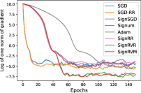
(a) $U=10$

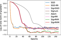
(b) $U=20$

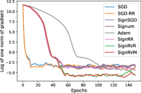
(c) $U=30$

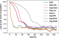
(d) $U=10$

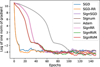
(e) $U=20$

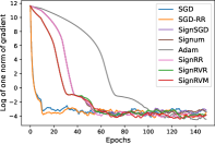
(f) $U=30$

Figure 1: Averaged results over 5 independent repetitions in the centralized setting with different data variances. (a)-(c): SignRR, SignRVR and SignRVM with a constant learning rate. (d)-(f): SignRR, SignRVR and SignRVM with a diminishing learning rate. SignRVR and SignRVM achieve the best results in all settings.

7.1.2 Distributed Setting

Implementation

For the distributed setting, we fix $U=10$, $n_{0}=1000$ and study the performance of optimizers under $M=10,20,30$. We are interested in the value decent along epochs. For better illustration, we take the logarithm of the function value and use the moving average with window size $7$ in visualization. The results are presented in Figure 2. It can be concluded that SignSGD with majority vote performs the worst. dist-SignRVR and dist-SignRVM have marginal advantages compared with other baseline methods.

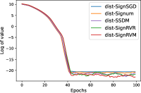
(a) $M=10$

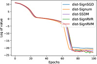
(b) $M=20$

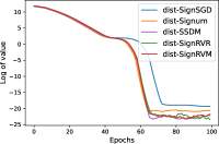
(c) $M=30$

Figure 2: Averaged results over 5 independent repetitions in the distributed setting with diminishing numbers of workers. dist-SignRVR and dist-SignRVM match SSDM’s performance and outperform others as $M$ increases.

7.2 Additional Experiments on MNIST Dataset

Now we compare our proposed algorithms with baseline algorithms on training a single-layer neural network on the MNIST dataset (LeCun et al., 1998) under the centralized setting and the distributed setting, respectively. Note that all optimizers use mini-batches for training. We aim to investigate the impact of different batch sizes under the centralized setting, and the impact of the number of workers under the distributed setting on our optimizers.

7.2.1 Centralized Setting

Implementation

We use the logistic function as the loss function. We study three different settings in which the batch size each algorithm uses in each iteration varies, falling within the range $\{32,64,128\}$. Similar to the previous experiment, we tune the constant learning rate of all methods using values from the range $\{1e-1,1e-2,1e-3,1e-4,1e-5,1e-6,1e-7\}$ and tune the momentum parameter in the range $\{0.1,0.2,0.3,0.4,0.5,0.6,0.7,0.8,0.9\}$. We use the default value $\beta_{2}=0.999$ for Adam. The test accuracies of different algorithms on MNIST are presented in Figure 3. We have the following observations:

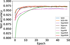
(a) Batch size $=32$

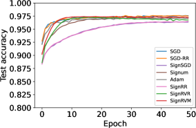
(b) Batch size $=64$

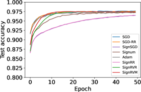
(c) Batch size $=128$

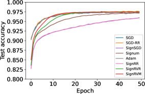
(d) Batch size $=256$

Figure 3: The test accuracies of experiment results on MNIST under the centralized setting with different batch sizes. Results are averaged over $5$ independent repetitions.

Comparing SignRR with signSGD

The experimental results show that no matter with a small batch size like 32 or 64, or a large batch size like 128 or 256, the test accuracy of SignRR matches that of signSGD. Furthermore, by only using the sign of gradients instead of the magnitudes of gradients, the results of SignRR are still comparable with the RR results when the batch size is larger than 64.

Comparing SignRVR with signSGD, SignRR

We observe that SignRVR beats SignRR and signSGD, and matches the performance of Adam. Moreover, SignRVR converges faster than Signum in a large batch size regime.

Comparing SignRVM with all sign based algorithms

Finally, SignRVM always performs well, outperforming all the sign-based algorithms and matching the performance of Adam. SignRVM, which only uses the signs of momentum to update, could also match RR and SGD, which use not only the signs but also the magnitudes of gradients to update.

7.2.2 Distributed Setting

Implementation For the distributed scenario, we study three different settings with the numbers of workers $M$ set to $5,10,$ and $20$ respectively, while keeping the batch size fixed at 64. The parameters are tuned similarly to those in the centralized setting.

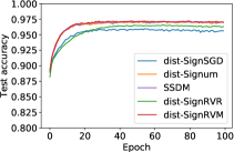
(a) $M=5$

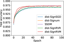
(b) $M=10$

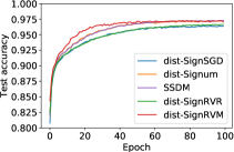
(c) $M=20$

Figure 4: The test accuracies of experiment results on MNIST under the distributed setting with different numbers of workers and fixed batch size 64. Results are averaged over $5$ independent repetitions.

The results on test accuracy are presented in Figure 4. It can be seen that dist-SignRVM, SIGNUM with majority vote and SSDM perform the best. When the number of workers is larger than 10, dist-SignRVM converges faster than Signum and SSDM. dist-SignRVR slightly outperforms SignSGD in all settings but is worse than those momentum based methods.

8 Conclusions

We presented the first convergence result for signSGD with random reshuffling, viz., SignRR, which matches the convergence rate of signSGD under the with-replacement sampling scheme. We proposed SignRVR that uses variance reduced gradients and SignRVM that uses momentum updates, which enhanced empirical performance compared with SignRR. In contrast with existing analyses of signSGD, our results do not need an extremely large mini-batch size to be of the same order as the total number of iterations (Bernstein et al., 2018) or the unrealistic SPB assumption (Safaryan and Richtárik, 2021). We further extended our algorithms to the distributed setting where data are stored across different machines, and provide corresponding convergence results. The experiments back up our theoretical results effectively. It remains an interesting open problem to show whether sign-based gradient methods under random reshuffling can provably outperform their with-replacement counterparts.

Appendix A Proof of The Main Theory

In this section, we prove our main theoretical results. First, we present the technical lemmas that would be useful throughout our proof.

Lemma A.1.

Given variable $b\in\mathbb{R}^{d}$, for any random variable $a\in\mathbb{R}^{d}$, we have

$$\mathbb{P}(\mathop{\mathrm{sign}}(a_{j})\neq\mathop{\mathrm{sign}}(b_{j}))\leq\frac{\mathbb{E}[|a_{j}-b_{j}|]}{|b_{j}|},$$

where $a_{j}$ and $b_{j}$ are the $j^{th}$ components of the vectors $a$ and $b$, respectively.

We use this lemma to calculate the probability that the estimators get a wrong sign of the true gradient, which is inspired by Bernstein et al. (2018).

Lemma A.2.

Consider the algorithm updated by $\mathbf{x}^{i+1}_{t}=\mathbf{x}^{i}_{t}-\gamma_{t}^{i}\mathop{\mathrm{sign}}(V(\mathbf{x}_{t}^{i}))$, where $\gamma_{t}^{i}$ is the learning rate and $V:\mathbb{R}^{d}\rightarrow\mathbb{R}^{d}$ is a measurable and square integrable function, we have

$$f(\mathbf{x}_{t}^{i+1})-f(\mathbf{x}_{t}^{i}) \leq-\gamma_{t}^{i}\lVert\nabla f(\mathbf{x}_{t}^{i})\rVert_{1}+\frac{(\gamma_{t}^{i})^{2}}{2}\lVert L\rVert_{1}$$

$$\qquad+2\gamma_{t}^{i}\sum_{j=1}^{d}\big{|}[\nabla f(\mathbf{x}_{t}^{i})]_{j}\big{|}\operatorname*{\mathds{1}}\big{\{}\mathop{\mathrm{sign}}([V(\mathbf{x}_{t}^{i})]_{j})\neq\mathop{\mathrm{sign}}([\nabla f(\mathbf{x}_{t}^{i})]_{j})\big{\}},$$

where $\operatorname*{\mathds{1}}\{\cdot\}$ is the indicator function.

This lemma is one of our fundamental techniques to prove the convergence rate of sign-based SGD. It suggests that the difference of the value function between two consecutive iterates relates to the $\ell_{1}$-norm of the true gradient, the Lipschitz constant, and the absolute value of the true gradient in the dimension where the signs of the estimated gradient and the true gradient are different.

Now we are ready to present the proof of our main theorems, which follows the generalized proof frame of sign gradient methods proposed by Bernstein et al. (2018).

A.1 Proof of Theorem 3.4

Proof.

According to the update rule in Algorithm 1, for the $i^{th}$ iteration in the $t^{th}$ epoch, we have

$$\mathbf{x}^{i+1}_{t}=\mathbf{x}^{i}_{t}-\gamma_{t}^{i}\mathop{\mathrm{sign}}(\nabla f_{\pi^{t}_{i}}(\mathbf{x}_{t}^{i})).$$

Then by Lemma A.2, we can derive

$$f(\mathbf{x}_{t}^{i+1})-f(\mathbf{x}_{t}^{i}) \leq-\gamma_{t}^{i}\lVert\nabla f(\mathbf{x}_{t}^{i})\rVert_{1}+\frac{(\gamma_{t}^{i})^{2}}{2}\lVert L\rVert_{1}$$

$$\qquad+2\gamma_{t}^{i}\sum_{j=1}^{d}\big{|}[\nabla f(\mathbf{x}_{t}^{i})]_{j}\big{|}\operatorname*{\mathds{1}}\big{\{}\mathop{\mathrm{sign}}([\nabla f_{\pi^{t}_{i}}(\mathbf{x}_{t}^{i})]_{j})\neq\mathop{\mathrm{sign}}([\nabla f(\mathbf{x}_{t}^{i})]_{j})\big{\}}.$$ (A.1)

Now we look at the individual terms in (A.1). Finding the expectation of improvement for the ${(i+1)}^{th}$ iteration conditioned on the previous iterate $\mathbf{x}_{t}^{i}$:

$$\mathbb{E}\big{[}f(\mathbf{x}_{t}^{i+1})-f(\mathbf{x}_{t}^{i})|\mathbf{x}_{t}^{i}\big{]} \leq-\gamma_{t}^{i}\lVert\nabla f(\mathbf{x}_{t}^{i})\rVert_{1}+\frac{(\gamma_{t}^{i})^{2}}{2}\lVert L\rVert_{1}$$

$$\qquad+2\gamma_{t}^{i}\sum_{j=1}^{d}\big{|}[\nabla f(\mathbf{x}_{t}^{i})]_{j}\big{|}\mathbb{P}\big{(}\mathop{\mathrm{sign}}([\nabla f_{\pi^{t}_{i}}(\mathbf{x}_{t}^{i})]_{j})\neq\mathop{\mathrm{sign}}([\nabla f(\mathbf{x}_{t}^{i})]_{j})|\mathbf{x}_{t}^{i}\big{)}.$$ (A.2)

Under Assumption 3.3, for the $j^{th}$ coordinate, the variance is bounded:

$$\mathbb{E}\big{[}([\nabla f_{\pi^{t}_{i}}(\mathbf{x}_{t}^{i})]_{j}-[\nabla f(\mathbf{x}_{t}^{i})]_{j})^{2}\big{]}\leq\sigma_{j}^{2}.$$ (A.3)

Then we focus on the probability that the estimators get a wrong sign of the true gradient. By using Lemma A.1, we obtain

$$\mathbb{P}\big{(}\mathop{\mathrm{sign}}([\nabla f_{\pi^{t}_{i}}(\mathbf{x}_{t}^{i})]_{j})\neq\mathop{\mathrm{sign}}([\nabla f(\mathbf{x}_{t}^{i})]_{j})|\mathbf{x}_{t}^{i}\big{)} \leq\frac{\mathbb{E}\big{[}|[\nabla f_{\pi^{t}_{i}}(\mathbf{x}_{t}^{i})]_{j}-[\nabla f(\mathbf{x}_{t}^{i})]_{j}|\big{]}}{\big{|}[\nabla f(\mathbf{x}_{t}^{i})]_{j}\big{|}}$$

$$\leq\frac{\sqrt{\mathbb{E}\big{[}([\nabla f_{\pi^{t}_{i}}(\mathbf{x}_{t}^{i})]_{j}-[\nabla f(\mathbf{x}_{t}^{i})]_{j})^{2}\big{]}}}{\big{|}[\nabla f(\mathbf{x}_{t}^{i})]_{j}\big{|}}$$

$$\overset{\eqref{eq:Var bounded}}{\leq}{\frac{|\sigma_{j}|}{\big{|}[\nabla f(\mathbf{x}_{t}^{i})]_{j}\big{|}}},$$ (A.4)

where the second inequality comes from Jensen’s inequality. Substituting (A.4) into (A.2),we have

$$\mathbb{E}\big{[}f(\mathbf{x}_{t}^{i+1})-f(\mathbf{x}_{t}^{i})|\mathbf{x}_{t}^{i}\big{]} \leq-\gamma_{t}^{i}\lVert\nabla f(\mathbf{x}_{t}^{i})\rVert_{1}+\frac{(\gamma_{t}^{i})^{2}}{2}\lVert L\rVert_{1}+2\gamma_{t}^{i}\sum_{j=1}^{d}\big{|}[\nabla f(\mathbf{x}_{t}^{i})]_{j}\big{|}\frac{|\sigma_{j}|}{\big{|}[\nabla f(\mathbf{x}_{t}^{i})]_{j}\big{|}}$$

$$=-\gamma_{t}^{i}\lVert\nabla f(\mathbf{x}_{t}^{i})\rVert_{1}+\frac{(\gamma_{t}^{i})^{2}}{2}\lVert L\rVert_{1}+2\gamma_{t}^{i}\sum_{j=1}^{d}|\sigma_{j}|$$

$$=-\gamma_{t}^{i}\lVert\nabla f(\mathbf{x}_{t}^{i})\rVert_{1}+\frac{(\gamma_{t}^{i})^{2}}{2}\lVert L\rVert_{1}+2\gamma_{t}^{i}\lVert\sigma\rVert_{1}.$$

Rearranging it, we get

$$\gamma_{t}^{i}\lVert\nabla f(\mathbf{x}_{t}^{i})\rVert_{1}\leq\mathbb{E}[f(\mathbf{x}_{t}^{i})-f(\mathbf{x}_{t}^{i+1})|\mathbf{x}_{t}^{i}]+\frac{(\gamma_{t}^{i})^{2}}{2}\lVert L\rVert_{1}+2\gamma_{t}^{i}\lVert\sigma\rVert_{1}.$$

In a single epoch, after $n$ iterations, a per-epoch recursion improvement satisfies

$$\sum_{i=0}^{n-1}\gamma_{t}^{i}\mathbb{E}\left[\lVert\nabla f(\mathbf{x}_{t}^{i})\rVert_{1}\right] \leq\sum_{i=0}^{n-1}\big{[}\mathbb{E}\big{[}f(\mathbf{x}_{t}^{i})\big{]}-\mathbb{E}\big{[}f(\mathbf{x}_{t}^{i+1})\big{]}+\frac{\lVert L\rVert_{1}}{2}\sum_{i=0}^{n-1}(\gamma_{t}^{i})^{2}+2\lVert\sigma\rVert_{1}\sum_{i=0}^{n-1}\gamma_{t}^{i}$$

$$\leq\mathbb{E}[f(\mathbf{x}_{t})]-\mathbb{E}[f(\mathbf{x}_{t+1})]+\frac{\lVert L\rVert_{1}}{2}\sum_{i=0}^{n-1}(\gamma_{t}^{i})^{2}+2\lVert\sigma\rVert_{1}\sum_{i=0}^{n-1}\gamma_{t}^{i}.$$

For $T$ epochs, we have

$$\sum_{t=0}^{T-1}\sum_{i=0}^{n-1}\gamma_{t}^{i}\mathbb{E}\left[\lVert\nabla f(\mathbf{x}_{t}^{i})\rVert_{1}\right] \leq\sum_{t=0}^{T-1}\mathbb{E}[f(\mathbf{x}_{t})]-\mathbb{E}[f(\mathbf{x}_{t+1})]+\frac{\lVert L\rVert_{1}}{2}\sum_{t=0}^{T-1}\sum_{i=0}^{n-1}(\gamma_{t}^{i})^{2}+2\lVert\sigma\rVert_{1}\sum_{t=0}^{T-1}\sum_{i=0}^{n-1}\gamma_{t}^{i}$$

$$\leq f(\mathbf{x}_{0})-\mathbb{E}\left[f(\mathbf{x}_{T})\right]+\frac{\lVert L\rVert_{1}}{2}\sum_{t=0}^{T-1}\sum_{i=0}^{n-1}(\gamma_{t}^{i})^{2}+2\lVert\sigma\rVert_{1}\sum_{t=0}^{T-1}\sum_{i=0}^{n-1}\gamma_{t}^{i}$$

$$\leq f(\mathbf{x}_{0})-f_{*}+\frac{\lVert L\rVert_{1}}{2}\sum_{t=0}^{T-1}\sum_{i=0}^{n-1}(\gamma_{t}^{i})^{2}+2\lVert\sigma\rVert_{1}\sum_{t=0}^{T-1}\sum_{i=0}^{n-1}\gamma_{t}^{i},$$ (A.5)

note that $x_{t}^{n}=x_{t+1}^{0}$. If we set the stepsize as $\gamma_{t}^{i}=\frac{\gamma_{0}}{\sqrt{nt+i+1}}$, then by (A.5), we have

$$\min_{0\leq i\leq n-1,0\leq t\leq T-1}\mathbb{E}\left[\lVert\nabla f(\mathbf{x}_{t}^{i})\rVert_{1}\right]\sum_{t=0}^{T-1}\sum_{i=0}^{n-1}\gamma_{t}^{i}\leq f(\mathbf{x}_{0})-f_{*}+\frac{\lVert L\rVert_{1}}{2}\sum_{t=0}^{T-1}\sum_{i=0}^{n-1}(\gamma_{t}^{i})^{2}+2\lVert\sigma\rVert_{1}\sum_{t=0}^{T-1}\sum_{i=0}^{n-1}\gamma_{t}^{i}.$$

Rearranging the result leads to

$$\min_{0\leq i\leq n-1,0\leq t\leq T-1}\mathbb{E}\left[\lVert\nabla f(\mathbf{x}_{t}^{i})\rVert_{1}\right]$$

$$\leq\frac{f(\mathbf{x}_{0})-f_{*}}{\sum_{t=0}^{T-1}\sum_{i=0}^{n-1}\gamma_{t}^{i}}+\frac{\lVert L\rVert_{1}}{2}\frac{\sum_{t=0}^{T-1}\sum_{i=0}^{n-1}(\gamma_{t}^{i})^{2}}{\sum_{t=0}^{T-1}\sum_{i=0}^{n-1}\gamma_{t}^{i}}+2\lVert\sigma\rVert_{1}\frac{\sum_{t=0}^{T-1}\sum_{i=0}^{n-1}\gamma_{t}^{i}}{\sum_{t=0}^{T-1}\sum_{i=0}^{n-1}\gamma_{t}^{i}}$$

$$\leq\frac{f(\mathbf{x}_{0})-f_{*}}{\sum_{k=0}^{nT-1}\frac{\gamma_{0}}{\sqrt{k+1}}}+\frac{\lVert L\rVert_{1}}{2}\frac{\sum_{k=0}^{nT-1}(\frac{\gamma_{0}}{\sqrt{k+1}})^{2}}{\sum_{k=0}^{nT-1}\frac{\gamma_{0}}{\sqrt{k+1}}}+2\lVert\sigma\rVert_{1}$$

$$\leq\frac{f(\mathbf{x}_{0})-f_{*}}{nT\frac{1}{\sqrt{nT}}\gamma_{0}}+\frac{\lVert L\rVert_{1}\gamma_{0}}{2}\frac{\log(nT)}{nT\frac{1}{\sqrt{nT}}}+2\lVert\sigma\rVert_{1}$$

$$=\frac{f(\mathbf{x}_{0})-f_{*}}{\sqrt{nT}\gamma_{0}}+\frac{\lVert L\rVert_{1}\gamma_{0}}{2}\frac{\log(nT)}{\sqrt{nT}}+2\lVert\sigma\rVert_{1},$$ (A.6)

where the third inequality holds by the fact that $\sum_{k=0}^{nT-1}\frac{1}{k+1}\leq\log(nT)$ and $\gamma_{t}^{i}\geq 1/\sqrt{nT}$. If we set the stepsize in Algorithm 1 as a constant stepsize $\gamma_{t}^{i}=\gamma$, then it holds that

$$\frac{1}{nT}\sum_{t=0}^{T-1}\sum_{i=0}^{n-1}\mathbb{E}\bigg{[}\lVert\nabla f(\mathbf{x}_{t}^{i})\rVert_{1}\bigg{]} \leq\frac{1}{nT\gamma}(f(\mathbf{x}_{0})-f(\mathbf{x}_{T}))+\frac{\gamma}{2}\lVert L\rVert_{1}+2\lVert\sigma\rVert_{1}$$

$$\leq\frac{1}{nT\gamma}(f(\mathbf{x}_{0})-f_{*})+\frac{\gamma}{2}\lVert L\rVert_{1}+2\lVert\sigma\rVert_{1},$$

which completes the proof. ∎

A.2 Proof of Theorem 4.1

Before we start to prove the convergence rate of Algorithm 2, we first state the lemmas that we will use later.

Every component difference between $\mathbf{x}_{t}^{i}$ and $\mathbf{y}_{t}$ is trivially bounded by following Lemma A.3.

Lemma A.3.

According to Algorithm 2, for every component of $\mathbf{x}_{t}^{i}-\mathbf{y}_{t}$ and with the diminishing stepsize $\gamma_{t}^{i}=\frac{\gamma_{0}}{\sqrt{nt+i+1}}$ or a constant stepsize $\gamma$, we have

$$\big{|}[\mathbf{x}_{t}^{i}]_{j}-[\mathbf{y}_{t}]_{j}\big{|}\leq\lVert\mathbf{x}_{t}^{i}-\mathbf{y}_{t}\rVert_{\infty}\leq D_{t}^{i}.$$

Lemma A.4 describes the fundamental property of the variance reduction part and bounds the difference between the estimate gradient $\big{(}[\nabla f_{\pi^{t}_{i}}(\mathbf{x}_{t}^{i})]_{j}-[\nabla f_{\pi^{t}_{i}}(\mathbf{y}_{t})]_{j}+[\nabla f(\mathbf{y}_{t})]_{j}\big{)}$ and the true gradient $[\nabla f(\mathbf{x}_{t}^{i})]_{j}$ by using the smoothness property of functions. Once we have this lemma, it is useful to notice that we do not need Assumption 3.3 anymore.

Lemma A.4.

According to Algorithm 2, with the diminishing stepsize $\gamma_{t}^{i}=\frac{\gamma_{0}}{\sqrt{nt+i+1}}$ or a constant stepsize $\gamma$, we have

$$\big{|}[\nabla f_{\pi^{t}_{i}}(\mathbf{x}_{t}^{i})]_{j}-[\nabla f_{\pi^{t}_{i}}(\mathbf{y}_{t})]_{j}+[\nabla f(\mathbf{y}_{t})]_{j}-[\nabla f(\mathbf{x}_{t}^{i})]_{j}\big{|}^{2}\leq 4L_{j}^{2}(D_{t}^{i})^{2}.$$

Now, we are ready to prove the convergence rate of Algorithm 2. The proof frame is the same as that of Theorem 3.4.

Proof of Theorem 4.1.

By using the estimate gradient $\big{(}\nabla f_{\pi^{t}_{i}}(\mathbf{x}_{t}^{i})-\nabla f_{\pi^{t}_{i}}(\mathbf{y}_{t})+\nabla f(\mathbf{y}_{t})\big{)}$, we obtain the update rule as

$$\mathbf{x}^{i+1}_{t}=\mathbf{x}^{i}_{t}-\gamma_{t}^{i}\mathop{\mathrm{sign}}(\nabla f_{\pi^{t}_{i}}(\mathbf{x}_{t}^{i})-\nabla f_{\pi^{t}_{i}}(\mathbf{y}_{t})+\nabla f(\mathbf{y}_{t})).$$

Note that with our choice of $D_{0}$, it is guaranteed that $\|\mathbf{x}_{t}^{i}-\mathbf{y}_{t}\|_{\infty}\leq D_{t}^{i}$ is true, thus Line 7 in Algorithm 2 is always executed. Then for any $t$ and $i$, by Lemma A.2, we have

$$f(\mathbf{x}_{t}^{i+1})-f(\mathbf{x}_{t}^{i}) \leq-\gamma_{t}^{i}\lVert\nabla f(\mathbf{x}_{t}^{i})\rVert_{1}+\frac{(\gamma_{t}^{i})^{2}}{2}\lVert L\rVert_{1}+2\gamma_{t}^{i}\sum_{j=1}^{d}\big{|}[\nabla f(\mathbf{x}_{t}^{i})]_{j}\big{|}\times$$

$$\qquad\operatorname*{\mathds{1}}\big{\{}\mathop{\mathrm{sign}}([\nabla f_{\pi^{t}_{i}}(\mathbf{x}_{t}^{i})]_{j}-[\nabla f_{\pi^{t}_{i}}(\mathbf{y}_{t})]_{j}+[\nabla f(\mathbf{y}_{t})]_{j})\neq\mathop{\mathrm{sign}}([\nabla f(\mathbf{x}_{t}^{i})]_{j})\big{\}}.$$ (A.7)

By using Lemmas A.1, A.3 and A.4, the probability that the estimators get a wrong sign of the true gradient yields

$$\mathbb{P}\big{(}\mathop{\mathrm{sign}}([\nabla f_{\pi^{t}_{i}}(\mathbf{x}_{t}^{i})]_{j}-[\nabla f_{\pi^{t}_{i}}(\mathbf{y}_{t})]_{j}+[\nabla f(\mathbf{y}_{t})]_{j})\neq\mathop{\mathrm{sign}}([\nabla f(\mathbf{x}_{t}^{i})]_{j})|\mathbf{x}_{t}^{i}\big{)}$$

$$\leq\frac{\mathbb{E}\big{[}|[\nabla f_{\pi^{t}_{i}}(\mathbf{x}_{t}^{i})]_{j}-[\nabla f_{\pi^{t}_{i}}(\mathbf{y}_{t})]_{j}+[\nabla f(\mathbf{y}_{t})]_{j}-[\nabla f(\mathbf{x}_{t}^{i})]_{j}|\big{]}}{\big{|}[\nabla f(\mathbf{x}_{t}^{i})]_{j}\big{|}}$$

$$\leq\frac{\sqrt{\mathbb{E}\big{[}([\nabla f_{\pi^{t}_{i}}(\mathbf{x}_{t}^{i})]_{j}-[\nabla f_{\pi^{t}_{i}}(\mathbf{y}_{t})]_{j}+[\nabla f(\mathbf{y}_{t})]_{j}-[\nabla f(\mathbf{x}_{t}^{i})]_{j})^{2}\big{]}}}{\big{|}[\nabla f(\mathbf{x}_{t}^{i})]_{j}\big{|}}$$

$$\leq\frac{2L_{j}D_{t}^{i}}{\big{|}[\nabla f(\mathbf{x}_{t}^{i})]_{j}\big{|}},$$

where the second inequality comes from Jensen’s inequality. Plugging it into (A.7) and taking expectation of (A.7) conditioned on $\mathbf{x}_{t}^{i}$, we have

$$\mathbb{E}[f(\mathbf{x}_{t}^{i+1})-f(\mathbf{x}_{t}^{i})|\mathbf{x}_{t}^{i}] \leq-\gamma_{t}^{i}\lVert\nabla f(\mathbf{x}_{t}^{i})\rVert_{1}+\frac{(\gamma_{t}^{i})^{2}}{2}\lVert L\rVert_{1}+2\gamma_{t}^{i}\sum_{j=1}^{d}\big{|}[\nabla f(\mathbf{x}_{t}^{i})]_{j}\big{|}\frac{2L_{j}D_{t}^{i}}{\big{|}[\nabla f(\mathbf{x}_{t}^{i})]_{j}\big{|}}$$

$$\leq-\gamma_{t}^{i}\lVert\nabla f(\mathbf{x}_{t}^{i})\rVert_{1}+\frac{(\gamma_{t}^{i})^{2}}{2}\lVert L\rVert_{1}+4\gamma_{t}^{i}D_{t}^{i}\lVert L\rVert_{1}.$$

Rearranging it, we can get

$$\gamma_{t}^{i}\lVert\nabla f(\mathbf{x}_{t}^{i})\rVert_{1}\leq\mathbb{E}[f(\mathbf{x}_{t}^{i})-f(\mathbf{x}_{t}^{i+1})|\mathbf{x}_{t}^{i}]+\frac{(\gamma_{t}^{i})^{2}}{2}\lVert L\rVert_{1}+4\gamma_{t}^{i}D_{t}^{i}\lVert L\rVert_{1}.$$

A per-epoch recursion improvement is showed as

$$\sum_{i=0}^{n-1}\gamma_{t}^{i}\mathbb{E}\left[\lVert\nabla f(\mathbf{x}_{t}^{i})\rVert_{1}\right] \leq\sum_{i=0}^{n-1}\big{[}\mathbb{E}\big{[}f(\mathbf{x}_{t}^{i})\big{]}-\mathbb{E}\big{[}f(\mathbf{x}_{t}^{i+1})\big{]}+\frac{\lVert L\rVert_{1}}{2}\sum_{i=0}^{n-1}(\gamma_{t}^{i})^{2}+4\lVert L\rVert_{1}\sum_{i=0}^{n-1}\gamma_{t}^{i}D_{t}^{i}$$

$$\leq\mathbb{E}[f(\mathbf{x}_{t})]-\mathbb{E}[f(\mathbf{x}_{t+1})]+\frac{\lVert L\rVert_{1}}{2}\sum_{i=0}^{n-1}(\gamma_{t}^{i})^{2}+4\lVert L\rVert_{1}\sum_{i=0}^{n-1}\gamma_{t}^{i}D_{t}^{i}.$$ (A.8)

For $T$ epochs, using (A.8), we get

$$\sum_{t=0}^{T-1}\sum_{i=0}^{n-1}\gamma_{t}^{i}\mathbb{E}\left[\lVert\nabla f(\mathbf{x}_{t}^{i})\rVert_{1}\right] \leq\sum_{t=0}^{T-1}\mathbb{E}[f(\mathbf{x}_{t})]-\mathbb{E}[f(\mathbf{x}_{t+1})]+\frac{\lVert L\rVert_{1}}{2}\sum_{t=0}^{T-1}\sum_{i=0}^{n-1}(\gamma_{t}^{i})^{2}+4\lVert L\rVert_{1}\sum_{t=0}^{T-1}\sum_{i=0}^{n-1}\gamma_{t}^{i}D_{t}^{i}$$

$$\leq f(\mathbf{x}_{0})-\mathbb{E}\left[f(\mathbf{x}_{T})\right]+\frac{\lVert L\rVert_{1}}{2}\sum_{t=0}^{T-1}\sum_{i=0}^{n-1}(\gamma_{t}^{i})^{2}+4\lVert L\rVert_{1}\sum_{t=0}^{T-1}\sum_{i=0}^{n-1}\gamma_{t}^{i}D_{t}^{i}$$

$$\leq f(\mathbf{x}_{0})-f_{*}+\frac{\lVert L\rVert_{1}}{2}\sum_{t=0}^{T-1}\sum_{i=0}^{n-1}(\gamma_{t}^{i})^{2}+4\lVert L\rVert_{1}\sum_{t=0}^{T-1}\sum_{i=0}^{n-1}\gamma_{t}^{i}D_{t}^{i}.$$ (A.9)

If we set the stepsize as $\gamma_{t}^{i}=\frac{\gamma_{0}}{\sqrt{nt+i+1}}$, then by (A.9), we have

$$\min_{0\leq i\leq n-1,0\leq t\leq T-1}\mathbb{E}\left[\lVert\nabla f(\mathbf{x}_{t}^{i})\rVert_{1}\right]\sum_{t=0}^{T-1}\sum_{i=0}^{n-1}\gamma_{t}^{i}\leq f(\mathbf{x}_{0})-f_{*}+\frac{\lVert L\rVert_{1}}{2}\sum_{t=0}^{T-1}\sum_{i=0}^{n-1}(\gamma_{t}^{i})^{2}+4\lVert L\rVert_{1}\sum_{t=0}^{T-1}\sum_{i=0}^{n-1}\gamma_{t}^{i}D_{t}^{i}.$$

Rearranging the result and setting $D_{t}^{i}=\frac{D_{0}}{\sqrt{nt+i+1}}$ leads to

$$\min_{0\leq i\leq n-1,0\leq t\leq T-1}\mathbb{E}\left[\lVert\nabla f(\mathbf{x}_{t}^{i})\rVert_{1}\right]$$

$$\leq\frac{f(\mathbf{x}_{0})-f_{*}}{\sum_{t=0}^{T-1}\sum_{i=0}^{n-1}\gamma_{t}^{i}}+\frac{\lVert L\rVert_{1}}{2}\frac{\sum_{t=0}^{T-1}\sum_{i=0}^{n-1}(\gamma_{t}^{i})^{2}}{\sum_{t=0}^{T-1}\sum_{i=0}^{n-1}\gamma_{t}^{i}}+4\lVert L\rVert_{1}\frac{\sum_{t=0}^{T-1}\sum_{i=0}^{n-1}\gamma_{t}^{i}D_{t}^{i}}{\sum_{t=0}^{T-1}\sum_{i=0}^{n-1}\gamma_{t}^{i}},$$

$$\leq\frac{f(\mathbf{x}_{0})-f_{*}}{\sum_{k=0}^{nT-1}\frac{\gamma_{0}}{\sqrt{k+1}}}+\frac{\lVert L\rVert_{1}}{2}\frac{\sum_{k=0}^{nT-1}(\frac{\gamma_{0}}{\sqrt{k+1}})^{2}}{\sum_{k=0}^{nT-1}\frac{\gamma_{0}}{\sqrt{k+1}}}+4\lVert L\rVert_{1}\frac{\sum_{k=0}^{nT-1}\frac{\gamma_{0}D_{0}}{k+1}}{\sum_{k=0}^{nT-1}\frac{\gamma_{0}}{\sqrt{k+1}}}$$

$$\leq\frac{f(\mathbf{x}_{0})-f_{*}}{nT\frac{1}{\sqrt{nT}}\gamma_{0}}+\frac{\lVert L\rVert_{1}}{2}\frac{\sum_{k=0}^{nT-1}\frac{\gamma_{0}^{2}}{k+1}}{nT\frac{1}{\sqrt{nT}}\gamma_{0}}+4\lVert L\rVert_{1}\frac{\sum_{k=0}^{nT-1}\frac{\gamma_{0}D_{0}}{k+1}}{nT\frac{1}{\sqrt{nT}}\gamma_{0}}$$

$$\leq\frac{f(\mathbf{x}_{0})-f_{*}}{\sqrt{nT}\gamma_{0}}+\frac{\lVert L\rVert_{1}\gamma_{0}}{2}\frac{\log(nT)}{\sqrt{nT}}+4\lVert L\rVert_{1}D_{0}\frac{\log(nT)}{\sqrt{nT}},$$

where the third inequality holds by the fact that $\gamma_{t}^{i}\geq 1/\sqrt{nT}$ and the last inequality holds by the fact that $\sum_{k=0}^{nT-1}\frac{1}{k+1}\leq\log(nT)$. If we further set the stepsize in Algorithm 2 as a constant stepsize $\gamma_{t}^{i}=\gamma$ and $D_{t}^{i}=D$, then it holds that

$$\frac{1}{nT}\sum_{t=0}^{T-1}\mathbb{E}\bigg{[}\sum_{i=0}^{n-1}\lVert\nabla f(\mathbf{x}_{t}^{i})\rVert_{1}\bigg{]} \leq\frac{1}{nT\gamma}(f(\mathbf{x}_{0})-f(\mathbf{x}_{T}))+\frac{\gamma}{2}\lVert L\rVert_{1}+4D\lVert L\rVert_{1}$$

$$\leq\frac{1}{nT\gamma}(f(\mathbf{x}_{0})-f_{*})+\frac{\gamma}{2}\lVert L\rVert_{1}+4D\lVert L\rVert_{1}.$$ (A.10)

This completes the proof. ∎

A.3 Proof of Theorem 5.1

We formulate the core lemmas and definitions for the proof of Theorem 5.1 first.

Definition A.5.

Following the proof of Signum in Bernstein et al. (2018), we recall the definition of random variables used in SignRVM:

$$g_{t}^{i} :=\nabla f(\mathbf{x}_{t}^{i}),$$

$$\tilde{g}_{t}^{i} :=\nabla f_{\pi^{t}_{i}}(\mathbf{x}_{t}^{i})-\nabla f_{\pi^{t}_{i}}(\mathbf{y}_{t})+\nabla f(\mathbf{y}_{t}),$$

$${q}_{t}^{i} :=\frac{1-\beta}{1-\beta^{i+1}}\sum_{p=0}^{i}[\beta^{p}g_{t}^{i-p}],$$

$$\tilde{q}_{t}^{i} :=\frac{1-\beta}{1-\beta^{i+1}}\sum_{p=0}^{i}[\beta^{p}\tilde{g}_{t}^{i-p}].$$

Note that inspired by Adam, we also multiply the coefficient $\frac{1}{1-\beta^{i+1}}$ to the momentum to correct the bias (Kingma and Ba, 2015), which will not inflect the signs of the momentum and final results.

Lemma A.6.

For all $i\in[n]$, by Definition A.5 and according to Algorithm 3, with $D_{t}^{i}=\frac{D_{0}}{\sqrt{n(t+1)+i+1}}$, we get

$$\sum_{j=1}^{d}\mathbb{E}\big{[}|[\tilde{q}_{t}^{i}]_{j}-[{q}_{t}^{i}]_{j}|\big{]}\leq\frac{2}{1-\beta}\frac{D_{0}}{\sqrt{n(t+1)}}\lVert L\rVert_{1}.$$

This lemma delineates the difference between the true and the estimated momentum, which will also be used to calculate the probability that the sign of the estimated gradient’s component is different from the sign of the true gradient’s component. We use Lemma A.4 to reduce the variance instead of directly using the gradient variance, thus getting rid of Assumption 3.3.

Lemma A.7.

For all $i\in[n]$, by Definition A.5 and according to Algorithm 3, with $D_{t}^{i}=\frac{D_{0}}{\sqrt{n(t+1)+i+1}}$, we have

$$\sum_{j=1}^{d}\mathbb{E}\big{[}|[{q}_{t}^{i}]_{j}-[g_{t}^{i}]_{j}|\big{]}\leq 2\lVert L\rVert_{1}\frac{D_{0}}{\sqrt{n(t+1)}}\frac{\beta}{(1-\beta)^{2}}.$$

This lemma delineates the difference between the true momentum and the true gradient, which also will be used to calculate the probability that the estimators get a wrong sign of the true gradient.

Now we start to prove Theorem 5.1.

Proof of Theorem 5.1.

According to the update rule in Algorithm 3, for the $i^{th}$ iteration in the $t^{th}$ epoch, we have

$$\mathbf{x}^{i+1}_{t}=\mathbf{x}^{i}_{t}-\gamma_{t}^{i}\mathop{\mathrm{sign}}(\tilde{q}_{t}^{i}).$$

Following the same proof structure of Algorithm 1 and Algorithm 2, and using Lemma A.2, we can derive

$$f(\mathbf{x}_{t}^{i+1})-f(\mathbf{x}_{t}^{i}) \leq-\gamma_{t}^{i}\lVert\nabla f(\mathbf{x}_{t}^{i})\rVert_{1}+\frac{(\gamma_{t}^{i})^{2}}{2}\lVert L\rVert_{1}$$

$$\qquad+2\gamma_{t}^{i}\sum_{j=1}^{d}\big{|}[\nabla f(\mathbf{x}_{t}^{i})]_{j}\big{|}\operatorname*{\mathds{1}}\big{\{}\mathop{\mathrm{sign}}([\tilde{q}_{t}^{i}]_{j})\neq\mathop{\mathrm{sign}}([\nabla f(\mathbf{x}_{t}^{i})]_{j})\big{\}}.$$

Taking the expectation of improvement for the ${i+1}^{th}$ iteration conditioned on the previous iterate $\mathbf{x}_{t}^{i}$:

$$\mathbb{E}\big{[}f(\mathbf{x}_{t}^{i+1})-f(\mathbf{x}_{t}^{i})|\mathbf{x}_{t}^{i}\big{]} \leq-\gamma_{t}^{i}\lVert\nabla f(\mathbf{x}_{t}^{i})\rVert_{1}+\frac{(\gamma_{t}^{i})^{2}}{2}\lVert L\rVert_{1}$$

$$\qquad+2\gamma_{t}^{i}\sum_{j=1}^{d}\big{|}[\nabla f(\mathbf{x}_{t}^{i})]_{j}\big{|}\mathbb{P}\big{(}\mathop{\mathrm{sign}}([\tilde{q}_{t}^{i}]_{j})\neq\mathop{\mathrm{sign}}([\nabla f(\mathbf{x}_{t}^{i})]_{j})|\mathbf{x}_{t}^{i}\big{)}.$$ (A.11)

For the diminishing stepsize $\gamma_{t}^{i}$, we finish the proof as follows. By using Lemma A.1, the probability that the estimators get a wrong sign of the true gradient is

$$\mathbb{P}\big{(}\mathop{\mathrm{sign}}([\tilde{q}_{t}^{i}]_{j})\neq\mathop{\mathrm{sign}}([\nabla f(\mathbf{x}_{t}^{i})]_{j})|\mathbf{x}_{t}^{i}\big{)}\leq\frac{\mathbb{E}[|[\tilde{q}_{t}^{i}]_{j}-[\nabla f(\mathbf{x}_{t}^{i})]_{j}|]}{\big{|}[\nabla f(\mathbf{x}_{t}^{i})]_{j}\big{|}}.$$ (A.12)

Considering the upper bound of $\mathbb{E}\big{[}|[\tilde{q}_{t}^{i}]_{j}-[\nabla f(\mathbf{x}_{t}^{i})]_{j}|\big{]}$, we have

$$\mathbb{E}\big{[}|[\tilde{q}_{t}^{i}]_{j}-[\nabla f(\mathbf{x}_{t}^{i})]_{j}|\big{]}\leq\mathbb{E}\big{[}|[\tilde{q}_{t}^{i}]_{j}-[{q}_{t}^{i}]_{j}|\big{]}+\mathbb{E}\big{[}|[{q}_{t}^{i}]_{j}-[\nabla f(\mathbf{x}_{t}^{i})]_{j}|\big{]}.$$

By using Lemmas A.7 and A.6, we can get

$$\sum_{j=1}^{d}\mathbb{E}\big{[}|[\tilde{q}_{t}^{i}]_{j}-[\nabla f(\mathbf{x}_{t}^{i})]_{j}|\big{]} \leq\sum_{j=1}^{d}\mathbb{E}\big{[}|[\tilde{q}_{t}^{i}]_{j}-[{q}_{t}^{i}]_{j}|\big{]}+\sum_{j=1}^{d}\mathbb{E}\big{[}|[{q}_{t}^{i}]_{j}-[\nabla f(\mathbf{x}_{t}^{i})]_{j}|\big{]}$$

$$\leq\frac{2}{1-\beta}\frac{D_{0}}{\sqrt{n(t+1)}}\lVert L\rVert_{1}+2\lVert L\rVert_{1}\frac{D_{0}}{\sqrt{n(t+1)}}\frac{\beta}{(1-\beta)^{2}}$$

$$=2\bigg{(}\frac{1}{1-\beta}+\frac{\beta}{(1-\beta)^{2}}\bigg{)}\lVert L\rVert_{1}\frac{D_{0}}{\sqrt{n(t+1)}}.$$ (A.13)

Substituting (A.13) and (A.12) to (A.11), we have

$$\mathbb{E}\big{[}f(\mathbf{x}_{t}^{i+1})-f(\mathbf{x}_{t}^{i})|\mathbf{x}_{t}^{i}\big{]}$$

$$\leq-\gamma_{t}^{i}\lVert\nabla f(\mathbf{x}_{t}^{i})\rVert_{1}+\frac{(\gamma_{t}^{i})^{2}}{2}\lVert L\rVert_{1}+2\gamma_{t}^{i}\sum_{j=1}^{d}\big{|}[\nabla f(\mathbf{x}_{t}^{i})]_{j}\big{|}\mathbb{P}\big{(}\mathop{\mathrm{sign}}([\tilde{q}_{t}^{i}]_{j})\neq\mathop{\mathrm{sign}}([\nabla f(\mathbf{x}_{t}^{i})]_{j})|\mathbf{x}_{t}^{i}\big{)}$$

$$\leq-\gamma_{t}^{i}\lVert\nabla f(\mathbf{x}_{t}^{i})\rVert_{1}+\frac{(\gamma_{t}^{i})^{2}}{2}\lVert L\rVert_{1}+4\gamma_{t}^{i}\bigg{(}\frac{1}{1-\beta}+\frac{\beta}{(1-\beta)^{2}}\bigg{)}\lVert L\rVert_{1}\frac{D_{0}}{\sqrt{n(t+1)}}.$$ (A.14)

Rearranging it, we can get

$$\gamma_{t}^{i}\lVert\nabla f(\mathbf{x}_{t}^{i})\rVert_{1}\leq\mathbb{E}[f(\mathbf{x}_{t}^{i})-f(\mathbf{x}_{t}^{i+1})|\mathbf{x}_{t}^{i}]+\frac{(\gamma_{t}^{i})^{2}}{2}\lVert L\rVert_{1}+4\gamma_{t}^{i}\bigg{(}\frac{1}{1-\beta}+\frac{\beta}{(1-\beta)^{2}}\bigg{)}\lVert L\rVert_{1}\frac{D_{0}}{\sqrt{n(t+1)}}.$$

For each epoch, we have

$$\sum_{i=0}^{n-1}\gamma_{t}^{i}\mathbb{E}\left[\lVert\nabla f(\mathbf{x}_{t}^{i})\rVert_{1}\right]$$

$$\leq\sum_{i=0}^{n-1}\big{[}\mathbb{E}\big{[}f(\mathbf{x}_{t}^{i})\big{]}-\mathbb{E}\big{[}f(\mathbf{x}_{t}^{i+1})\big{]}+\frac{\lVert L\rVert_{1}}{2}\sum_{i=0}^{n-1}(\gamma_{t}^{i})^{2}+4\bigg{(}\frac{1}{1-\beta}+\frac{\beta}{(1-\beta)^{2}}\bigg{)}\lVert L\rVert_{1}\sum_{i=0}^{n-1}\gamma_{t}^{i}\frac{D_{0}}{\sqrt{n(t+1)}}$$

$$\leq\mathbb{E}[f(\mathbf{x}_{t})]-\mathbb{E}[f(\mathbf{x}_{t+1})]+\frac{\lVert L\rVert_{1}}{2}\sum_{i=0}^{n-1}(\gamma_{t}^{i})^{2}+4\bigg{(}\frac{1}{1-\beta}+\frac{\beta}{(1-\beta)^{2}}\bigg{)}\lVert L\rVert_{1}\sum_{i=0}^{n-1}\gamma_{t}^{i}\frac{D_{0}}{\sqrt{n(t+1)}}.$$ (A.15)

For all the epochs, we have

$$\sum_{t=0}^{T-1}\sum_{i=0}^{n-1}\gamma_{t}^{i}\mathbb{E}\left[\lVert\nabla f(\mathbf{x}_{t}^{i})\rVert_{1}\right]$$

$$\leq\sum_{t=0}^{T-1}\mathbb{E}[f(\mathbf{x}_{t})]-\mathbb{E}[f(\mathbf{x}_{t+1})]+\frac{\lVert L\rVert_{1}}{2}\sum_{t=0}^{T-1}\sum_{i=0}^{n-1}(\gamma_{t}^{i})^{2}+4\bigg{(}\frac{1}{1-\beta}+\frac{\beta}{(1-\beta)^{2}}\bigg{)}\lVert L\rVert_{1}\sum_{t=0}^{T-1}\sum_{i=0}^{n-1}\frac{\gamma_{t}^{i}D_{0}}{\sqrt{n(t+1)}}$$

$$\leq f(\mathbf{x}_{0})-\mathbb{E}\left[f(\mathbf{x}_{T})\right]+\frac{\lVert L\rVert_{1}}{2}\sum_{t=0}^{T-1}\sum_{i=0}^{n-1}(\gamma_{t}^{i})^{2}+4\bigg{(}\frac{1}{1-\beta}+\frac{\beta}{(1-\beta)^{2}}\bigg{)}\lVert L\rVert_{1}\sum_{t=0}^{T-1}\sum_{i=0}^{n-1}\frac{\gamma_{t}^{i}D_{0}}{\sqrt{n(t+1)}}$$

$$\leq f(\mathbf{x}_{0})-f_{*}+\frac{\lVert L\rVert_{1}}{2}\sum_{t=0}^{T-1}\sum_{i=0}^{n-1}(\gamma_{t}^{i})^{2}+4\bigg{(}\frac{1}{1-\beta}+\frac{\beta}{(1-\beta)^{2}}\bigg{)}\lVert L\rVert_{1}\sum_{t=0}^{T-1}\sum_{i=0}^{n-1}\frac{\gamma_{t}^{i}D_{0}}{\sqrt{n(t+1)}}.$$ (A.16)

Then by (A.16), we have

$$\min_{0\leq i\leq n-1,0\leq t\leq T-1}\mathbb{E}\left[\lVert\nabla f(\mathbf{x}_{t}^{i})\rVert_{1}\right]\sum_{t=0}^{T-1}\sum_{i=0}^{n-1}\gamma_{t}^{i}$$

$$\leq f(\mathbf{x}_{0})-f_{*}+\frac{\lVert L\rVert_{1}}{2}\sum_{t=0}^{T-1}\sum_{i=0}^{n-1}(\gamma_{t}^{i})^{2}+4\bigg{(}\frac{1}{1-\beta}+\frac{\beta}{(1-\beta)^{2}}\bigg{)}\lVert L\rVert_{1}\sum_{t=0}^{T-1}\sum_{i=0}^{n-1}\gamma_{t}^{i}\frac{D_{0}}{\sqrt{n(t+1)}}.$$

Rearranging the result leads to

$$\min_{0\leq i\leq n-1,0\leq t\leq T-1}\mathbb{E}\left[\lVert\nabla f(\mathbf{x}_{t}^{i})\rVert_{1}\right]$$

$$\leq\frac{f(\mathbf{x}_{0})-f_{*}}{\sum_{t=0}^{T-1}\sum_{i=0}^{n-1}\gamma_{t}^{i}}+\frac{\lVert L\rVert_{1}}{2}\frac{\sum_{t=0}^{T-1}\sum_{i=0}^{n-1}(\gamma_{t}^{i})^{2}}{\sum_{t=0}^{T-1}\sum_{i=0}^{n-1}\gamma_{t}^{i}}+4\bigg{(}\frac{1}{1-\beta}+\frac{\beta}{(1-\beta)^{2}}\bigg{)}\lVert L\rVert_{1}\frac{\sum_{t=0}^{T-1}\sum_{i=0}^{n-1}\gamma_{t}^{i}\frac{D_{0}}{\sqrt{n(t+1)}}}{\sum_{t=0}^{T-1}\sum_{i=0}^{n-1}\gamma_{t}^{i}}.$$

If we set the stepsize as $\gamma_{t}^{i}=\frac{\gamma_{0}}{\sqrt{n(t+1)+i+1}}$, then we have

$$\sum_{t=0}^{T-1}\sum_{i=0}^{n-1}\gamma_{t}^{i}=\sum_{t=0}^{T-1}\sum_{i=0}^{n-1}\frac{\gamma_{0}}{\sqrt{n(t+1)+i+1}}\geq\frac{\gamma_{0}nT}{\sqrt{n(T+1)}}\geq\frac{1}{2}\frac{\gamma_{0}n(T+1)}{\sqrt{n(T+1)}}=\frac{\gamma_{0}}{2}\sqrt{n(T+1)}.$$ (A.18)

Let us further bound $\sum_{t=0}^{T-1}\sum_{i=0}^{n-1}(\gamma_{t}^{i})^{2}$ as following:

$$\sum_{t=0}^{T-1}\sum_{i=0}^{n-1}(\gamma_{t}^{i})^{2}=\sum_{t=0}^{T-1}\sum_{i=0}^{n-1}(\frac{\gamma_{0}}{\sqrt{n(t+1)+i+1}})^{2}\leq\sum_{t=0}^{T-1}\sum_{i=0}^{n-1}\frac{\gamma_{0}^{2}}{nt+i+1}\leq\sum_{k=0}^{nT-1}\frac{\gamma_{0}^{2}}{k+1}\leq\gamma_{0}^{2}\log(nT).$$ (A.19)

By using $\sum_{t=0}^{T-1}\frac{1}{t+1}\leq\log T$ for the last inequality, we also get

$$\sum_{t=0}^{T-1}\sum_{i=0}^{n-1}\gamma_{t}^{i}\frac{D_{0}}{\sqrt{n(t+1)}} \leq\sum_{t=0}^{T-1}\sum_{i=0}^{n-1}\frac{\gamma_{0}}{\sqrt{n(t+1)+i+1}}\frac{D_{0}}{\sqrt{n(t+1)}}$$

$$\leq\sum_{t=0}^{T-1}\sum_{i=0}^{n-1}\frac{\gamma_{0}}{\sqrt{n(t+1)}}\frac{D_{0}}{\sqrt{n(t+1)}}$$

$$\leq\sum_{t=0}^{T-1}\frac{\gamma_{0}D_{0}}{t+1}$$

$$\leq\gamma_{0}D_{0}\log(T).$$ (A.20)

Incorporating (A.18), (A.19) and (A.20) into (LABEL:eq:rvm_min), we deduce

$$\min_{0\leq i\leq n-1,0\leq t\leq T-1}\mathbb{E}\left[\lVert\nabla f(\mathbf{x}_{t}^{i})\rVert_{1}\right]$$

$$\leq\frac{2(f(\mathbf{x}_{0})-f_{*})}{\sqrt{n(T+1)}\gamma_{0}}+\lVert L\rVert_{1}\frac{\gamma_{0}^{2}\log(nT)}{\sqrt{n(T+1)}\gamma_{0}}+8\bigg{(}\frac{1}{1-\beta}+\frac{\beta}{(1-\beta)^{2}}\bigg{)}\lVert L\rVert_{1}\frac{\gamma_{0}D_{0}\log(T)}{\sqrt{n(T+1)}\gamma_{0}}$$

$$\leq\frac{2(f(\mathbf{x}_{0})-f_{*})}{\sqrt{nT}\gamma_{0}}+\lVert L\rVert_{1}\gamma_{0}\frac{\log(nT)}{\sqrt{nT}}+8\bigg{(}\frac{1}{1-\beta}+\frac{\beta}{(1-\beta)^{2}}\bigg{)}\lVert L\rVert_{1}D_{0}\frac{\log(T)}{\sqrt{nT}}.$$

Then, let us consider the proof of convergence result with the constant stepsize $\gamma$ and $D$. By using Lemmas A.7 and A.6, we can get

$$\frac{1}{nT}\sum_{t=0}^{T-1}\mathbb{E}\bigg{[}\sum_{i=0}^{n-1}\lVert\nabla f(\mathbf{x}_{t}^{i})\rVert_{1}\bigg{]} \leq\frac{1}{nT\gamma}(f(\mathbf{x}_{0})-f(\mathbf{x}_{T}))+\frac{\gamma}{2}\lVert L\rVert_{1}+4D\bigg{(}\frac{1}{1-\beta}+\frac{\beta}{(1-\beta)^{2}}\bigg{)}\lVert L\rVert_{1}$$

$$\leq\frac{1}{nT\gamma}(f(\mathbf{x}_{0})-f_{*})+\frac{\gamma}{2}\lVert L\rVert_{1}+4D\bigg{(}\frac{1}{1-\beta}+\frac{\beta}{(1-\beta)^{2}}\bigg{)}\lVert L\rVert_{1}.$$

This completes the proof. ∎

A.4 Proof of Theorem 6.2

Prior to commencing the proof of the convergence rate of Theorem 6.2, we present the lemma that will be utilized later in the analysis.

Lemma A.8.

(Safaryan and Richtárik, 2021, Lemma 15) For any non-zero vectors $a$ and $b$,

$$-\frac{\langle a,b\rangle}{\lVert a\rVert}\leq-\frac{1}{3}\lVert b\rVert+\frac{8}{3}\lVert a-b\rVert.$$

Let us now proceed with the proof of Theorem 6.2.

Proof.

By using the estimated gradient $s_{t,i}:=\frac{1}{M}\sum_{m=1}^{M}s_{t,i}^{m}$ and the smoothness of $f^{m}(\mathbf{x})$, we obtain

$$f(\mathbf{x}_{t}^{i+1}) =\frac{1}{M}\sum_{m=1}^{M}f^{m}(\mathbf{x}_{t}^{i+1})$$

$$\leq\frac{1}{M}\sum_{m=1}^{M}\Bigg{[}f^{m}(\mathbf{x}_{t}^{i})-\gamma_{t}^{i}\langle\nabla f^{m}(\mathbf{x}_{t}^{i}),s_{t,i}\rangle+\frac{{L}(\gamma_{t}^{i})^{2}}{2}\bigg{\lVert}\frac{1}{M}\sum_{m=1}^{M}s_{t,i}^{m}\bigg{\rVert}_{2}^{2}\Bigg{]}$$

$$\leq f(\mathbf{x}_{t}^{i})+\frac{1}{M}\sum_{m=1}^{M}\Bigg{[}-\gamma_{t}^{i}\langle\nabla f^{m}(\mathbf{x}_{t}^{i}),s_{t,i}\rangle+\frac{{L}(\gamma_{t}^{i})^{2}}{2}\frac{1}{M}\sum_{m=1}^{M}\lVert s_{t,i}^{m}\rVert_{2}^{2}\Bigg{]}$$

$$=f(\mathbf{x}_{t}^{i})+\frac{1}{M}\sum_{m=1}^{M}\Bigg{[}-\frac{\gamma_{t}^{i}}{M}\sum_{m=1}^{M}\langle\nabla f^{m}(\mathbf{x}_{t}^{i}),s_{t,i}^{m}\rangle\Bigg{]}+\frac{d{L}(\gamma_{t}^{i})2}{2}.$$

Taking expectation conditioned on the previous iterate $\mathbf{x}_{t}^{i}$, by Lemma A.8, we get

$$\mathbb{E}[f(\mathbf{x}_{t}^{i+1})|\mathbf{x}_{t}^{i}]$$

$$\leq f(\mathbf{x}_{t}^{i})+\frac{1}{M}\sum_{m=1}^{M}\Bigg{[}-\frac{\gamma_{t}^{i}}{M}\sum_{m=1}^{M}\frac{\langle\nabla f^{m}(\mathbf{x}_{t}^{i}),\nabla f^{m}_{\pi_{i}^{t}}(\mathbf{x}_{t}^{i})-\nabla f^{m}_{\pi_{i}^{t}}(\mathbf{y}_{t})+\nabla f^{m}(\mathbf{y}_{t})\rangle}{\lVert\nabla f^{m}_{\pi_{i}^{t}}(\mathbf{x}_{t}^{i})-\nabla f^{m}_{\pi_{i}^{t}}(\mathbf{y}_{t})+\nabla f^{m}(\mathbf{y}_{t})\rVert_{2}}\Bigg{]}+\frac{d{L}(\gamma_{t}^{i})^{2}}{2}$$

$$\leq f(\mathbf{x}_{t}^{i})+\frac{1}{M}\sum_{m=1}^{M}\Bigg{[}-\frac{\gamma_{t}^{i}}{3M}\sum_{m=1}^{M}\lVert\nabla f^{m}(\mathbf{x}_{t}^{i})\rVert_{2}+\frac{8\gamma_{t}^{i}}{3M}\sum_{m=1}^{M}\lVert\nabla f^{m}_{\pi_{i}^{t}}(\mathbf{x}_{t}^{i})-\nabla f^{m}_{\pi_{i}^{t}}(\mathbf{y}_{t})$$

$$\qquad+\nabla f^{m}(\mathbf{y}_{t})-\nabla f^{m}(\mathbf{x}_{t}^{i})\rVert_{2}\Bigg{]}+\frac{d{L}(\gamma_{t}^{i})^{2}}{2}$$

$$\leq f(\mathbf{x}_{t}^{i})+\frac{1}{M}\sum_{m=1}^{M}\Bigg{[}-\frac{\gamma_{t}^{i}}{3}\lVert\nabla f(\mathbf{x}_{t}^{i})\rVert_{2}+\frac{8\gamma_{t}^{i}}{3M}\sum_{m=1}^{M}\lVert\nabla f^{m}_{\pi_{i}^{t}}(\mathbf{x}_{t}^{i})-\nabla f^{m}_{\pi_{i}^{t}}(\mathbf{y}_{t})$$

$$\qquad+\nabla f^{m}(\mathbf{y}_{t})-\nabla f^{m}(\mathbf{x}_{t}^{i})\rVert_{2}\Bigg{]}+\frac{d{L}(\gamma_{t}^{i})^{2}}{2},$$ (A.21)

where the last inequality is due to $\lVert\nabla f(\mathbf{x}_{t}^{i})\rVert_{2}=\lVert\frac{1}{M}\sum_{m=1}^{M}\nabla f^{m}(\mathbf{x}_{t}^{i})\rVert_{2}\leq\frac{1}{M}\sum_{m=1}^{M}\lVert\nabla f^{m}(\mathbf{x}_{t}^{i})\rVert_{2}$. To bound $\lVert\nabla f^{m}_{\pi_{i}^{t}}(\mathbf{x}_{t}^{i})-\nabla f^{m}_{\pi_{i}^{t}}(\mathbf{y}_{t})+\nabla f^{m}(\mathbf{y}_{t})-\nabla f^{m}(\mathbf{x}_{t}^{i})\rVert_{2}$, we have

$$\lVert\nabla f^{m}_{\pi_{i}^{t}}(\mathbf{x}_{t}^{i})-\nabla f^{m}_{\pi_{i}^{t}}(\mathbf{y}_{t})+\nabla f^{m}(\mathbf{y}_{t})-\nabla f^{m}(\mathbf{x}_{t}^{i})\rVert_{2}$$

$$\leq\lVert\nabla f^{m}_{\pi_{i}^{t}}(\mathbf{x}_{t}^{i})-\nabla f^{m}_{\pi_{i}^{t}}(\mathbf{y}_{t})\rVert_{2}+\lVert\nabla f^{m}(\mathbf{y}_{t})-\nabla f^{m}(\mathbf{x}_{t}^{i})\rVert_{2}$$

$$\leq 2L\lVert\mathbf{x}_{t}^{i}-\mathbf{y}_{t}\rVert_{2}$$

$$\leq 2\sqrt{d}LD_{t}^{i},$$ (A.22)

where the first inequality is a result of the triangle inequality, and the second inequality follows from the smoothness of $f_{i}(\mathbf{x})$. Incorporating (A.22) into (A.21) and rearranging it, we can derive

$${\gamma_{t}^{i}}\lVert\nabla f(\mathbf{x}_{t}^{i})\rVert_{2} \leq 3\mathbb{E}[f(\mathbf{x}_{t}^{i})-f(\mathbf{x}_{t}^{i+1})|\mathbf{x}_{t}^{i}]+\frac{16{\gamma_{t}^{i}}}{M}\sqrt{d}\sum_{m=1}^{M}LD_{t}^{i}+\frac{3dL(\gamma_{t}^{i})^{2}}{2}$$

$$=3\mathbb{E}[f(\mathbf{x}_{t}^{i})-f(\mathbf{x}_{t}^{i+1})|\mathbf{x}_{t}^{i}]+16{\gamma_{t}^{i}}\sqrt{d}LD_{t}^{i}+\frac{3dL(\gamma_{t}^{i})^{2}}{2}.$$

In a single epoch, after ${n_{0}}$ iterations, a per-epoch recursion improvement satisfies

$$\sum_{i=0}^{n_{0}-1}\gamma_{t}^{i}\mathbb{E}\left[\lVert\nabla f(\mathbf{x}_{t}^{i})\rVert_{2}\right] \leq 3\sum_{i=0}^{n_{0}-1}\big{[}\mathbb{E}\big{[}f(\mathbf{x}_{t}^{i})\big{]}-\mathbb{E}\big{[}f(\mathbf{x}_{t}^{i+1})\big{]}\big{]}+\frac{3dL}{2}\sum_{i=0}^{n_{0}-1}(\gamma_{t}^{i})^{2}+16\sqrt{d}L\sum_{i=0}^{n_{0}-1}\gamma_{t}^{i}D_{t}^{i}$$

$$\leq 3\left(\mathbb{E}[f(\mathbf{x}_{t})]-\mathbb{E}[f(\mathbf{x}_{t+1})]\right)+\frac{3dL}{2}\sum_{i=0}^{n_{0}-1}(\gamma_{t}^{i})^{2}+16\sqrt{d}L\sum_{i=0}^{n_{0}-1}\gamma_{t}^{i}D_{t}^{i}.$$

For $T$ epochs, the recursion improvement for all epochs is ensured

$$\sum_{t=0}^{T-1}\sum_{i=0}^{n_{0}-1}\gamma_{t}^{i}\mathbb{E}\left[\lVert\nabla f(\mathbf{x}_{t}^{i})\rVert_{2}\right]$$

$$\leq\sum_{t=0}^{T-1}3\left(\mathbb{E}[f(\mathbf{x}_{t})]-\mathbb{E}[f(\mathbf{x}_{t+1})]\right)+\frac{3dL}{2}\sum_{t=0}^{T-1}\sum_{i=0}^{n_{0}-1}(\gamma_{t}^{i})^{2}+16\sqrt{d}L\sum_{t=0}^{T-1}\sum_{i=0}^{n_{0}-1}\gamma_{t}^{i}D_{t}^{i}$$

$$\leq 3\left(f(\mathbf{x}_{0})-\mathbb{E}\left[f(\mathbf{x}_{T})\right]\right)+\frac{3dL}{2}\sum_{t=0}^{T-1}\sum_{i=0}^{n_{0}-1}(\gamma_{t}^{i})^{2}+16\sqrt{d}L\sum_{t=0}^{T-1}\sum_{i=0}^{n_{0}-1}\gamma_{t}^{i}D_{t}^{i}$$

$$\leq 3\left(f(\mathbf{x}_{0})-f_{*}\right)+\frac{3dL}{2}\sum_{t=0}^{T-1}\sum_{i=0}^{n_{0}-1}(\gamma_{t}^{i})^{2}+16\sqrt{d}L\sum_{t=0}^{T-1}\sum_{i=0}^{n_{0}-1}\gamma_{t}^{i}D_{t}^{i}.$$ (A.23)

If we set the stepsize as $\gamma_{t}^{i}=\frac{\gamma_{0}}{\sqrt{n_{0}t+i+1}}$, then by (A.23), we have

$$\min_{0\leq i\leq n_{0}-1,0\leq t\leq T-1}\mathbb{E}\left[\lVert\nabla f(\mathbf{x}_{t}^{i})\rVert_{2}\right]\sum_{t=0}^{T-1}\sum_{i=0}^{n_{0}-1}\gamma_{t}^{i}$$

$$\leq 3(f(\mathbf{x}_{0})-f_{*})+\frac{3dL}{2}\sum_{t=0}^{T-1}\sum_{i=0}^{n_{0}-1}(\gamma_{t}^{i})^{2}+16\sqrt{d}L\sum_{t=0}^{T-1}\sum_{i=0}^{n_{0}-1}\gamma_{t}^{i}D_{t}^{i}.$$

Rearranging the result and setting $D_{t}^{i}=\frac{D_{0}}{\sqrt{n_{0}t+i+1}}$ leads to

$$\min_{0\leq i\leq n_{0}-1,0\leq t\leq T-1}\mathbb{E}\left[\lVert\nabla f(\mathbf{x}_{t}^{i})\rVert_{2}\right]$$

$$\leq\frac{3(f(\mathbf{x}_{0})-f_{*})}{\sum_{t=0}^{T-1}\sum_{i=0}^{n_{0}-1}\gamma_{t}^{i}}+\frac{3dL}{2}\frac{\sum_{t=0}^{T-1}\sum_{i=0}^{n_{0}-1}(\gamma_{t}^{i})^{2}}{\sum_{t=0}^{T-1}\sum_{i=0}^{n_{0}-1}\gamma_{t}^{i}}+16\sqrt{d}L\frac{\sum_{t=0}^{T-1}\sum_{i=0}^{n_{0}-1}\gamma_{t}^{i}D_{t}^{i}}{\sum_{t=0}^{T-1}\sum_{i=0}^{n_{0}-1}\gamma_{t}^{i}},$$

$$\leq\frac{3(f(\mathbf{x}_{0})-f_{*})}{\sum_{k=0}^{n_{0}T-1}\frac{\gamma_{0}}{\sqrt{k+1}}}+\frac{3dL}{2}\frac{\sum_{k=0}^{n_{0}T-1}(\frac{\gamma_{0}}{\sqrt{k+1}})^{2}}{\sum_{k=0}^{n_{0}T-1}\frac{\gamma_{0}}{\sqrt{k+1}}}+16\sqrt{d}L\frac{\sum_{k=0}^{n_{0}T-1}\frac{\gamma_{0}D_{0}}{k+1}}{\sum_{k=0}^{n_{0}T-1}\frac{\gamma_{0}}{\sqrt{k+1}}}$$

$$\leq\frac{3(f(\mathbf{x}_{0})-f_{*})}{n_{0}T\frac{1}{\sqrt{n_{0}T}}\gamma_{0}}+\frac{3dL}{2}\frac{\sum_{k=0}^{n_{0}T-1}\frac{\gamma_{0}^{2}}{k+1}}{n_{0}T\frac{1}{\sqrt{n_{0}T}}\gamma_{0}}+16\sqrt{d}L\frac{\sum_{k=0}^{n_{0}T-1}\frac{\gamma_{0}D_{0}}{k+1}}{n_{0}T\frac{1}{\sqrt{n_{0}T}}\gamma_{0}}$$

$$\leq\frac{3(f(\mathbf{x}_{0})-f_{*})}{\sqrt{n_{0}T}\gamma_{0}}+\frac{3dL}{2}\frac{\log(n_{0}T)\gamma_{0}}{\sqrt{n_{0}T}}+16\sqrt{d}LD_{0}\frac{\log(n_{0}T)}{\sqrt{n_{0}T}},$$

where the third inequality holds by the fact that $\gamma_{t}^{i}\geq 1/\sqrt{n_{0}T}$ and the last inequality holds by the fact that $\sum_{k=0}^{n_{0}T-1}\frac{1}{k+1}\leq\log(n_{0}T)$.

Assuming a constant stepsize $\gamma$ and a fixed value for $D$, the following result can be derived:

$$\frac{1}{n_{0}T}\sum_{t=0}^{T-1}\sum_{i=0}^{n_{0}-1}\mathbb{E}\left[\lVert\nabla f(\mathbf{x}_{t}^{i})\rVert_{2}\right] \leq\frac{3(f(\mathbf{x}_{0})-f_{*})}{n_{0}T\gamma}+\frac{3dL\gamma}{2}+16\sqrt{d}LD.$$

This completes the proof. ∎

A.5 Proof of Theorem 6.5

Proof.

Following the proof of SignRVM, we define similar notations as used in Definition A.5 for the centralized setting.

Definition A.9.

$g_{t,i}^{m}$, $\tilde{g}_{t,i}^{m}$, ${q}_{t,i}^{m}$ and $\tilde{q}_{t,i}^{m}$ are defined as following:

$$g_{t,i}^{m} :=\nabla f^{m}(\mathbf{x}_{t}^{i}),$$

$$\tilde{g}_{t,i}^{m} :=\nabla f^{m}_{\pi^{t}_{i}}(\mathbf{x}_{t}^{i})-\nabla f^{m}_{\pi^{t}_{i}}(\mathbf{y}_{t})+\nabla f^{m}(\mathbf{y}_{t}),$$

$${q}_{t,i}^{m} :=\frac{1-\beta}{1-\beta^{i+1}}\sum_{p=0}^{i}[\beta^{p}g_{t,i-p}^{m}],$$

$$\tilde{q}_{t,i}^{m} :=\frac{1-\beta}{1-\beta^{i+1}}\sum_{p=0}^{i}[\beta^{p}\tilde{g}_{t,i-p}^{m}].$$

Note that inspired by Adam, we also multiply the coefficient $\frac{1}{1-\beta^{i+1}}$ to the momentum to correct the bias (Kingma and Ba, 2015), which will not inflect the signs of the momentum and final results.

By using the estimate gradient $h_{t,i}:=\frac{1}{M}\sum_{m=1}^{M}h_{t,i}^{m}$ and the smoothness of $f^{m}(\mathbf{x})$, we obtain

$$f(\mathbf{x}_{t}^{i+1}) =\frac{1}{M}\sum_{m=1}^{M}f^{m}(\mathbf{x}_{t}^{i+1})$$

$$\leq\frac{1}{M}\sum_{m=1}^{M}\Bigg{[}f^{m}(\mathbf{x}_{t}^{i})-\gamma_{t}^{i}\langle\nabla f^{m}(\mathbf{x}_{t}^{i}),h_{t,i}\rangle+\frac{{L}(\gamma_{t}^{i})^{2}}{2}\bigg{\lVert}\frac{1}{M}\sum_{m=1}^{M}h_{t,i}^{m}\bigg{\rVert}_{2}^{2}\Bigg{]}$$

$$\leq f(\mathbf{x}_{t}^{i})+\frac{1}{M}\sum_{m=1}^{M}\Bigg{[}-\gamma_{t}^{i}\langle\nabla f^{m}(\mathbf{x}_{t}^{i}),h_{t,i}\rangle+\frac{{L}(\gamma_{t}^{i})^{2}}{2}\frac{1}{M}\sum_{m=1}^{M}\lVert h_{t,i}^{m}\rVert_{2}^{2}\Bigg{]}$$

$$=f(\mathbf{x}_{t}^{i})+\frac{1}{M}\sum_{m=1}^{M}\Bigg{[}-\frac{\gamma_{t}^{i}}{M}\sum_{m=1}^{M}\langle\nabla f^{m}(\mathbf{x}_{t}^{i}),h_{t,i}^{m}\rangle\Bigg{]}+\frac{d{L}(\gamma_{t}^{i})2}{2}.$$

Taking expectation conditioned on the previous iterate $\mathbf{x}_{t}^{i}$, by Lemma A.8, we get

$$\mathbb{E}[f(x_{t+1}^{i})|\mathbf{x}_{t}^{i}] \leq f(\mathbf{x}_{t}^{i})+\frac{1}{M}\sum_{m=1}^{M}\Bigg{[}-\frac{\gamma_{t}^{i}}{M}\sum_{m=1}^{M}\frac{\langle\nabla f^{m}(\mathbf{x}_{t}^{i}),\tilde{q}_{t,i}^{m}\rangle}{\lVert\tilde{q}_{t,i}^{m}\rVert_{2}}\Bigg{]}+\frac{d{L}(\gamma_{t}^{i})^{2}}{2}$$

$$\leq f(\mathbf{x}_{t}^{i})+\frac{1}{M}\sum_{m=1}^{M}\Bigg{[}-\frac{\gamma_{t}^{i}}{3M}\sum_{m=1}^{M}\lVert\nabla f^{m}(\mathbf{x}_{t}^{i})\rVert_{2}+\frac{8\gamma_{t}^{i}}{3M}\sum_{m=1}^{M}\lVert\tilde{q}_{t,i}^{m}-\nabla f^{m}(\mathbf{x}_{t}^{i})\rVert_{2}\Bigg{]}+\frac{d{L}(\gamma_{t}^{i})^{2}}{2}$$

$$\leq f(\mathbf{x}_{t}^{i})+\frac{1}{M}\sum_{m=1}^{M}\Bigg{[}-\frac{\gamma_{t}^{i}}{3}\lVert\nabla f(\mathbf{x}_{t}^{i})\rVert_{2}+\frac{8\gamma_{t}^{i}}{3M}\sum_{m=1}^{M}\lVert\tilde{q}_{t,i}^{m}-\nabla f^{m}(\mathbf{x}_{t}^{i})\rVert_{2}\Bigg{]}+\frac{d{L}(\gamma_{t}^{i})^{2}}{2},$$ (A.24)

where the last inequality follows from the triangle inequality such that

$$\lVert\nabla f(\mathbf{x}_{t}^{i})\rVert_{2}=\bigg{\lVert}\frac{1}{M}\sum_{m=1}^{M}\nabla f^{m}(\mathbf{x}_{t}^{i})\bigg{\rVert}_{2}\leq\frac{1}{M}\sum_{m=1}^{M}\lVert\nabla f^{m}(\mathbf{x}_{t}^{i})\rVert_{2}.$$

To bound $\lVert\tilde{q}_{t,i}^{m}-\nabla f^{m}(\mathbf{x}_{t}^{i})\rVert_{2}$, we have

$$\lVert\tilde{q}_{t,i}^{m}-\nabla f^{m}(\mathbf{x}_{t}^{i})\rVert_{2}\leq\lVert\tilde{q}_{t,i}^{m}-{q}_{t,i}^{m}\rVert_{2}+\lVert{q}_{t,i}^{m}-\nabla f^{m}(\mathbf{x}_{t}^{i})\rVert_{2}.$$

Note that in this proof, quantities like $Z_{t}^{i}$, $\lvert Z_{t}^{i}\rvert$, and $(Z_{t}^{i})^{2}$ are regarded as vectors. Consequently, this proof constitutes an assertion pertaining to each individual component of these vectors, and all operations, such as $(\cdot)^{2}$, are carried out element-wise. According to Definition A.9, we can bound $\lVert{q}_{t,i}^{m}-\nabla f^{m}(\mathbf{x}_{t}^{i})\rVert_{2}$ as follows:

$$\lVert{q}_{t,i}^{m}-\nabla f^{m}(\mathbf{x}_{t}^{i})\rVert_{2} =\lVert{q}_{t,i}^{m}-g_{t,i}^{m}\rVert_{2}$$

$$=\bigg{\lVert}\frac{1-\beta}{1-\beta^{i+1}}\sum_{p=1}^{i}\beta^{p}g_{t,i-p}^{m}-\frac{1-\beta}{1-\beta^{i+1}}\sum_{p=1}^{i}\beta^{p}g_{t,i}^{m}\bigg{\rVert}_{2}$$

$$\leq\frac{1-\beta}{1-\beta^{i+1}}\sum_{p=1}^{i}\beta^{p}\lVert g_{t,i-p}^{m}-g_{t,i}^{m}\rVert_{2}$$

$$\leq\sum_{p=1}^{i}\beta^{p}\lVert g_{t,i-p}^{m}-g_{t,i}^{m}\rVert_{2}.$$ (A.25)

By definition of $g_{t,i}^{m}$, we have

$$\lVert g_{t,i-p}^{m}-g_{t,i}^{m}\rVert_{2} =\lVert\nabla f^{m}(\mathbf{x}_{t}^{i-p})-\nabla f^{m}(\mathbf{x}_{t}^{i})\rVert_{2}\leq L\lVert\mathbf{x}_{t}^{i-p}-\mathbf{x}_{t}^{i}\rVert_{2}\leq 2\sqrt{d}L\sum_{l=1}^{p}D_{t}^{i-l}.$$ (A.26)

By setting $D_{t}^{i}=\frac{D_{0}}{\sqrt{n_{0}(t+1)+i+1}}$, we get

$$2\sqrt{d}L\sum_{l=1}^{p}D_{t}^{i-l}\leq 2\sqrt{d}L\sum_{l=1}^{p}\frac{D_{0}}{\sqrt{n_{0}(t+1)+i-l+1}}\leq 2\sqrt{d}L\sum_{l=1}^{p}\frac{D_{0}}{\sqrt{n_{0}(t+1)}}=2\sqrt{d}L\frac{D_{0}}{\sqrt{n_{0}(t+1)}}p.$$ (A.27)

Combining (A.27), (A.26) and (A.25), we have

$$\lVert{q}_{t,i}^{m}-\nabla f^{m}(\mathbf{x}_{t}^{i})\rVert_{2} \leq\frac{2\sqrt{d}LD_{0}}{\sqrt{n_{0}(t+1)}}\sum_{p=1}^{\infty}p\beta^{p}$$

$$\leq\frac{2\sqrt{d}LD_{0}}{\sqrt{n_{0}(t+1)}}\frac{\beta}{(1-\beta)^{2}},$$

where the second inequality is due to the derivative of geometric series. According to Definition A.9, we first define $Z_{t,i}^{m}:=\tilde{g}_{t,i}^{m}-g_{t,i}^{m}$. By using Jensen’s inequality and geometric series, we bound $\lVert\tilde{q}_{t,i}^{m}-{q}_{t,i}^{m}\rVert_{2}$ as follows

$$\lVert\tilde{q}_{t,i}^{m}-{q}_{t,i}^{m}\rVert_{2} =\frac{1-\beta}{1-\beta^{i+1}}\Bigg{\lVert}\sum_{p=0}^{i}\beta^{p}Z_{t,i-p}^{m}\Bigg{\rVert}_{2}\leq\frac{1-\beta}{1-\beta^{i+1}}\sqrt{\Bigg{\lVert}\sum_{p=0}^{i}\beta^{p}Z_{t,i-p}^{m}\Bigg{\rVert}_{2}^{2}}.$$ (A.28)

Considering $\big{(}\sum_{p=0}^{i}\beta^{p}[Z_{t,i-p}^{m}]_{j}\big{)}^{2}$ , we have

$$\Bigg{(}\sum_{p=0}^{i}\beta^{p}[Z_{t,i-p}^{m}]_{j}\Bigg{)}^{2}=\Bigg{(}\sum_{p=0}^{i}\frac{\beta^{p}}{\sum_{p=0}^{i}\beta^{p}}\Bigg{(}\sum_{p=0}^{i}\beta^{p}\Bigg{)}[Z_{t,i-p}^{m}]_{j}\Bigg{)}^{2}=\Bigg{(}\mathbb{E}\Bigg{[}\Bigg{(}\sum_{p=0}^{i}\beta^{p}\Bigg{)}[Z_{t,i-p}^{m}]_{j}\Bigg{]}\Bigg{)}^{2}.$$ (A.29)

By using $(\mathbb{E}\mathbf{x})^{2}\leq\mathbb{E}\mathbf{x}^{2}$, from (A.29), we have

$$\Bigg{(}\mathbb{E}\Bigg{[}\Bigg{(}\sum_{p=1}^{i}\beta^{p}\Bigg{)}[Z_{t,i-p}^{m}]_{j}\Bigg{]}\Bigg{)}^{2} \leq\mathbb{E}\Bigg{[}\Bigg{(}\sum_{p=1}^{i}\beta^{p}\Bigg{)}^{2}([Z_{t,i-p}^{m}]_{j})^{2}\Bigg{]}$$

$$=\sum_{p=1}^{i}\frac{\beta^{p}}{\sum_{p=1}^{i}\beta^{p}}\Bigg{(}\sum_{p=1}^{i}\beta^{p}\Bigg{)}^{2}([Z_{t,i-p}^{m}]_{j})^{2}$$

$$=\sum_{p=1}^{i}\beta^{p}\Bigg{(}\sum_{p=1}^{i}\beta^{p}\Bigg{)}([Z_{t,i-p}^{m}]_{j})^{2}.$$ (A.30)

We bound $[Z_{t,i}^{m}]_{j}:=[\tilde{g}_{t,i}^{m}]_{j}-[g_{t,i}^{m}]_{j}$ as follow,

$$\lvert[Z_{t,i}^{m}]_{j}\rvert^{2} =\lvert[\tilde{g}_{t,i}^{m}]_{j}-[g_{t,i}^{m}]_{j}\rvert^{2}$$

$$=\lvert[\nabla f^{m}_{\pi^{t}_{i}}(\mathbf{x}_{t}^{i})]_{j}-[\nabla f^{m}_{\pi^{t}_{i}}(\mathbf{y}_{t})]_{j}+[\nabla f^{m}(\mathbf{y}_{t})]_{j}-[\nabla f^{m}(\mathbf{x}_{t}^{i})]_{j}\rvert^{2}$$

$$\leq 4L^{2}(D_{t}^{i})^{2}.$$ (A.31)

where the last inequality is due to Lemma A.4. Incorporating (A.30) and (A.31), and using geometric series, we get

$$\sum_{l=1}^{i}\beta^{p}\Bigg{(}\sum_{p=0}^{i}\beta^{p}\Bigg{)}([Z_{t,i-p}^{m}]_{j})^{2} =\Bigg{(}\sum_{p=0}^{i}\beta^{p}\Bigg{)}\sum_{p=0}^{i}\beta^{p}([Z_{t,i-p}^{m}]_{j})^{2}$$

$$\leq\Bigg{(}\sum_{p=0}^{i}\beta^{p}\Bigg{)}\sum_{p=0}^{i}\beta^{p}4L^{2}(D_{t}^{i-p})^{2}$$

$$\leq\frac{1}{1-\beta}4L^{2}\sum_{p=0}^{i}\beta^{p}(D_{t}^{i-p})^{2}.$$ (A.32)

Thus, combining (A.28) and (A.32), we have

$$\lVert\tilde{q}_{t,i}^{m}-{q}_{t,i}^{m}\rVert_{2} \leq\frac{1-\beta}{1-\beta^{i+1}}\sqrt{\mathbb{E}\Bigg{[}\Bigg{\lVert}\sum_{p=0}^{i}\beta^{p}Z_{t,i-p}^{m}\Bigg{\rVert}_{2}^{2}\Bigg{]}}$$

$$\leq\frac{1-\beta}{1-\beta^{i+1}}\sqrt{\frac{1}{1-\beta}4dL^{2}\sum_{p=0}^{i}\beta^{p}(D_{t}^{i-p})^{2}}$$

$$=\frac{2\sqrt{d}L\sqrt{1-\beta}}{1-\beta^{i+1}}\sqrt{\sum_{p=0}^{i}\beta^{p}(D_{t}^{i-p})^{2}}.$$ (A.33)

By using geometric series and setting $D_{t}^{i}=\frac{D_{0}}{\sqrt{n_{0}(t+1)+i+1}}$, we get

$$\sum_{p=0}^{i}\beta^{p}(D_{t}^{i-p})^{2}=\sum_{p=0}^{i}\beta^{p}\frac{D_{0}^{2}}{{n_{0}(t+1)+i-p+1}}\leq\sum_{p=0}^{i}\beta^{p}\frac{D_{0}^{2}}{{n_{0}(t+1)}}\leq\frac{D_{0}^{2}}{{n_{0}(t+1)}}\frac{1}{1-\beta}.$$ (A.34)

Incorporating (A.33) and (A.34), we deduce

$$\lVert\tilde{q}_{t,i}^{m}-{q}_{t,i}^{m}\rVert_{2} \leq\frac{2\sqrt{d}L\sqrt{1-\beta}}{1-\beta^{i+1}}\sqrt{\sum_{p=0}^{i}\beta^{p}(D_{t}^{i-p})^{2}}$$

$$\leq\frac{2\sqrt{d}L\sqrt{1-\beta}}{1-\beta^{i+1}}\frac{D_{0}}{\sqrt{n_{0}(t+1)}}\frac{1}{\sqrt{1-\beta}}$$

$$\leq\frac{2}{1-\beta}\sqrt{d}L\frac{D_{0}}{\sqrt{n_{0}(t+1)}},$$ (A.35)

where the last inequality is due to $\frac{1}{1-\beta^{i+1}}\leq\frac{1}{1-\beta}$. Now, we have

$$\lVert\tilde{q}_{t,i}^{m}-\nabla f^{m}(\mathbf{x}_{t}^{i})\rVert_{2} \leq\lVert\tilde{q}_{t,i}^{m}-{q}_{t,i}^{m}\rVert_{2}+\lVert{q}_{t,i}^{m}-\nabla f^{m}(\mathbf{x}_{t}^{i})\rVert_{2}.$$

$$\leq\frac{2\sqrt{d}LD_{0}}{\sqrt{n_{0}(t+1)}(1-\beta)}+2\sqrt{d}L\frac{D_{0}}{\sqrt{n_{0}(t+1)}}\frac{\beta}{(1-\beta)^{2}}$$

$$=2\sqrt{d}L\frac{D_{0}}{\sqrt{n_{0}(t+1)}}\bigg{(}\frac{1}{1-\beta}+\frac{\beta}{(1-\beta)^{2}}\bigg{)}.$$ (A.36)

Combining (A.36) and (A.24) and rearranging it, we can get

$${\gamma_{t}^{i}}\lVert\nabla f(\mathbf{x}_{t}^{i})\rVert_{2}$$

$$\leq 3\mathbb{E}[f(\mathbf{x}_{t}^{i})-f(\mathbf{x}_{t+1}^{i})|\mathbf{x}_{t}]+\frac{16{\gamma_{t}^{i}}}{M}\sum_{m=1}^{M}\left(\sqrt{d}L\frac{D_{0}}{\sqrt{n_{0}(t+1)}}\bigg{(}\frac{1}{1-\beta}+\frac{\beta}{(1-\beta)^{2}}\bigg{)}\right)+\frac{3dL(\gamma_{t}^{i})^{2}}{2}$$

$$=3\mathbb{E}[f(\mathbf{x}_{t}^{i})-f(\mathbf{x}_{t+1}^{i})|\mathbf{x}_{t}^{i}]+16{\gamma_{t}^{i}}\sqrt{d}L\frac{D_{0}}{\sqrt{n_{0}(t+1)}}\bigg{(}\frac{1}{1-\beta}+\frac{\beta}{(1-\beta)^{2}}\bigg{)}+\frac{3dL(\gamma_{t}^{i})^{2}}{2}.$$

In a single epoch, after $n_{0}$ iterations, a per-epoch recursion improvement satisfies

$$\sum_{i=0}^{n_{0}-1}\gamma_{t}^{i}\mathbb{E}\left[\lVert\nabla f(\mathbf{x}_{t}^{i})\rVert_{2}\right] \leq 3\sum_{i=0}^{n_{0}-1}\big{[}\mathbb{E}\big{[}f(\mathbf{x}_{t}^{i})\big{]}-\mathbb{E}\big{[}f(\mathbf{x}_{t}^{i+1})\big{]}\big{]}+\frac{3dL}{2}\sum_{i=0}^{n_{0}-1}(\gamma_{t}^{i})^{2}$$

$$\qquad+16\sqrt{d}L\bigg{(}\frac{1}{1-\beta}+\frac{\beta}{(1-\beta)^{2}}\bigg{)}\frac{D_{0}}{\sqrt{n_{0}(t+1)}}\sum_{i=0}^{n_{0}-1}{\gamma_{t}^{i}}$$

$$\leq 3\left(\mathbb{E}[f(\mathbf{x}_{t})]-\mathbb{E}[f(\mathbf{x}_{t+1})]\right)+\frac{3dL}{2}\sum_{i=0}^{n_{0}-1}(\gamma_{t}^{i})^{2}$$

$$\qquad+16\sqrt{d}L\bigg{(}\frac{1}{1-\beta}+\frac{\beta}{(1-\beta)^{2}}\bigg{)}\frac{D_{0}}{\sqrt{n_{0}(t+1)}}\sum_{i=0}^{n_{0}-1}{\gamma_{t}^{i}}.$$

After $T$ epochs, we have

$$\sum_{t=0}^{T-1}\sum_{i=0}^{n_{0}-1}\gamma_{t}^{i}\mathbb{E}\left[\lVert\nabla f(\mathbf{x}_{t}^{i})\rVert_{2}\right] \leq\sum_{t=0}^{T-1}3\left(\mathbb{E}[f(\mathbf{x}_{t})]-\mathbb{E}[f(\mathbf{x}_{t+1})]\right)+\frac{3dL}{2}\sum_{t=0}^{T-1}\sum_{i=0}^{n_{0}-1}(\gamma_{t}^{i})^{2}$$

$$\qquad+16\sqrt{d}L\bigg{(}\frac{1}{1-\beta}+\frac{\beta}{(1-\beta)^{2}}\bigg{)}\sum_{t=0}^{T-1}\sum_{i=0}^{n_{0}-1}{\gamma_{t}^{i}}\frac{D_{0}}{\sqrt{n_{0}(t+1)}}$$

$$\leq 3\left(f(\mathbf{x}_{0})-\mathbb{E}\left[f(\mathbf{x}_{T})\right]\right)+\frac{3dL}{2}\sum_{t=0}^{T-1}\sum_{i=0}^{n_{0}-1}(\gamma_{t}^{i})^{2}$$

$$\qquad+16\sqrt{d}L\bigg{(}\frac{1}{1-\beta}+\frac{\beta}{(1-\beta)^{2}}\bigg{)}\sum_{t=0}^{T-1}\sum_{i=0}^{n_{0}-1}{\gamma_{t}^{i}}\frac{D_{0}}{\sqrt{n_{0}(t+1)}}$$

$$\leq 3\left(f(\mathbf{x}_{0})-f_{*}\right)+\frac{3dL}{2}\sum_{t=0}^{T-1}\sum_{i=0}^{n_{0}-1}(\gamma_{t}^{i})^{2}$$

$$\qquad+16\sqrt{d}L\bigg{(}\frac{1}{1-\beta}+\frac{\beta}{(1-\beta)^{2}}\bigg{)}\sum_{t=0}^{T-1}\sum_{i=0}^{n_{0}-1}{\gamma_{t}^{i}}\frac{D_{0}}{\sqrt{n_{0}(t+1)}}.$$

Then we further have

$$\min_{0\leq i\leq n_{0}-1,0\leq t\leq T-1}\mathbb{E}\left[\lVert\nabla f(\mathbf{x}_{t}^{i})\rVert_{2}\right]\sum_{t=0}^{T-1}\sum_{i=0}^{n_{0}-1}\gamma_{t}^{i}$$

$$\leq 3\left(f(\mathbf{x}_{0})-f_{*}\right)+\frac{3dL}{2}\sum_{t=0}^{T-1}\sum_{i=0}^{n_{0}-1}(\gamma_{t}^{i})^{2}+16\sqrt{d}L\bigg{(}\frac{1}{1-\beta}+\frac{\beta}{(1-\beta)^{2}}\bigg{)}\sum_{t=0}^{T-1}\sum_{i=0}^{n_{0}-1}{\gamma_{t}^{i}}\frac{D_{0}}{\sqrt{n_{0}(t+1)}}.$$

Rearranging the result leads to

$$\min_{0\leq i\leq n_{0}-1,0\leq t\leq T-1}\mathbb{E}\left[\lVert\nabla f(\mathbf{x}_{t}^{i})\rVert\right] \leq\frac{3(f(\mathbf{x}_{0})-f_{*})}{\sum_{t=0}^{T-1}\sum_{i=0}^{n_{0}-1}\gamma_{t}^{i}}+\frac{3dL}{2}\frac{\sum_{t=0}^{T-1}\sum_{i=0}^{n_{0}-1}(\gamma_{t}^{i})^{2}}{\sum_{t=0}^{T-1}\sum_{i=0}^{n_{0}-1}\gamma_{t}^{i}}$$

$$\qquad+16\sqrt{d}L\bigg{(}\frac{1}{1-\beta}+\frac{\beta}{(1-\beta)^{2}}\bigg{)}\frac{\sum_{t=0}^{T-1}\sum_{i=0}^{n_{0}-1}\gamma_{t}^{i}\frac{D_{0}}{\sqrt{n_{0}(t+1)}}}{\sum_{t=0}^{T-1}\sum_{i=0}^{n_{0}-1}\gamma_{t}^{i}}.$$ (A.37)

If we set the stepsize as $\gamma_{t}^{i}=\frac{\gamma_{0}}{\sqrt{n_{0}(t+1)+i+1}}$, then we have

$$\sum_{t=0}^{T-1}\sum_{i=0}^{n_{0}-1}\gamma_{t}^{i}=\sum_{t=0}^{T-1}\sum_{i=0}^{n_{0}-1}\frac{\gamma_{0}}{\sqrt{n_{0}(t+1)+i+1}}\geq\frac{\gamma_{0}n_{0}T}{\sqrt{n_{0}(T+1)}}\geq\frac{1}{2}\frac{\gamma_{0}n_{0}(T+1)}{\sqrt{n_{0}(T+1)}}=\frac{\gamma_{0}}{2}\sqrt{n_{0}(T+1)}.$$ (A.38)

Let us further bound $\sum_{t=0}^{T-1}\sum_{i=0}^{n-1}(\gamma_{t}^{i})^{2}$ as following:

$$\sum_{t=0}^{T-1}\sum_{i=0}^{n_{0}-1}(\gamma_{t}^{i})^{2}=\sum_{t=0}^{T-1}\sum_{i=0}^{n_{0}-1}\frac{\gamma_{0}^{2}}{n_{0}(t+1)+i+1}\leq\sum_{t=0}^{T-1}\sum_{i=0}^{n_{0}-1}\frac{\gamma_{0}^{2}}{n_{0}t+i+1}\leq\sum_{k=0}^{n_{0}T-1}\frac{\gamma_{0}^{2}}{k+1}\leq\gamma_{0}\log(n_{0}T).$$ (A.39)

By using the fact that $\sum_{t=0}^{T-1}\frac{1}{t+1}\leq\log T$ for the last inequality, we also get

$$\sum_{t=0}^{T-1}\sum_{i=0}^{n_{0}-1}\gamma_{t}^{i}\frac{D_{0}}{\sqrt{n_{0}(t+1)}} \leq\sum_{t=0}^{T-1}\sum_{i=0}^{n_{0}-1}\frac{\gamma_{0}}{\sqrt{n_{0}(t+1)+i+1}}\frac{D_{0}}{\sqrt{n_{0}(t+1)}}$$

$$\leq\sum_{t=0}^{T-1}\sum_{i=0}^{n_{0}-1}\frac{\gamma_{0}}{\sqrt{n_{0}(t+1)}}\frac{D_{0}}{\sqrt{n_{0}(t+1)}}$$

$$\leq\sum_{t=0}^{T-1}\frac{\gamma_{0}D_{0}}{t+1}$$

$$\leq\gamma_{0}D_{0}\log(T).$$ (A.40)

Incorporating (A.38), (A.39) and (A.40) into (A.37), we deduce

$$\min_{0\leq i\leq n_{0}-1,0\leq t\leq T-1}\mathbb{E}\left[\lVert\nabla f(\mathbf{x}_{t}^{i})\rVert_{2}\right]$$ (A.41)

$$\leq\frac{6(f(\mathbf{x}_{0})-f_{*})}{\sqrt{n_{0}(T+1)}\gamma_{0}}+3dL\gamma_{0}^{2}\frac{\log(n_{0}T)}{\sqrt{n_{0}(T+1)}\gamma_{0}}+32\sqrt{d}LD_{0}\bigg{(}\frac{1}{1-\beta}+\frac{\beta}{(1-\beta)^{2}}\bigg{)}\frac{\gamma_{0}\log(T)}{{\sqrt{n_{0}(T+1)}\gamma_{0}}},$$

$$\leq\frac{6(f(\mathbf{x}_{0})-f_{*})}{\sqrt{n_{0}T}\gamma_{0}}+3dL\gamma_{0}\frac{\log(n_{0}T)}{\sqrt{n_{0}T}}+32\sqrt{d}LD_{0}\bigg{(}\frac{1}{1-\beta}+\frac{\beta}{(1-\beta)^{2}}\bigg{)}\frac{\log(T)}{\sqrt{n_{0}T}}.$$

Assuming a constant stepsize $\gamma$ and a fixed value for $D$, the following result can be derived:

$$\frac{1}{n_{0}T}\sum_{t=0}^{T-1}\sum_{i=0}^{n_{0}-1}\mathbb{E}\left[\lVert\nabla f(\mathbf{x}_{t}^{i})\rVert_{2}\right] \leq\frac{3(f(\mathbf{x}_{0})-f_{*})}{n_{0}T\gamma}+\frac{3dL\gamma}{2}+16\sqrt{d}LD\bigg{(}\frac{1}{1-\beta}+\frac{\beta}{(1-\beta)^{2}}\bigg{)}.$$

This completes the proof. ∎

Appendix B Proof of Technical Lemmas

B.1 Proof of Lemma A.1

We first recall Lemma A.1 as follows. See A.1

Proof.

The proof follows immediately from Markov’s inequality for the last inequality.

$$\mathbb{P}(\mathop{\mathrm{sign}}(a_{j})\neq\mathop{\mathrm{sign}}(b_{j}))\leq\mathbb{P}\big{(}|a_{j}-b_{j}|\geq|b_{j}|\big{)}\leq\frac{\mathbb{E}[|a_{j}-b_{j}|]}{|b_{j}|},$$

which completes the proof. ∎

B.2 Proof of Lemma A.2

We restate the lemma as follows. See A.2

Proof.

For the $i^{th}$ iteration in the $t^{th}$ epoch, we generalize the update rule in Algorithms as

$$\mathbf{x}^{i+1}_{t}=\mathbf{x}^{i}_{t}-\gamma_{t}^{i}\mathop{\mathrm{sign}}(V(\mathbf{x}_{t}^{i})).$$

Since $f$ is $L$-smooth by Assumption 3.2, we can derive

$$f(\mathbf{x}_{t}^{i+1})-f(\mathbf{x}_{t}^{i}) \leq\langle\nabla f(\mathbf{x}_{t}^{i}),\mathbf{x}^{i+1}_{t}-\mathbf{x}_{t}^{i}\rangle+\sum_{j=1}^{d}\frac{L_{j}}{2}([\mathbf{x}^{i+1}_{t}]_{j}-[\mathbf{x}_{t}^{i}]_{j})^{2}$$

$$=-\gamma_{t}^{i}\langle\nabla f(\mathbf{x}_{t}^{i}),\mathop{\mathrm{sign}}(V(\mathbf{x}_{t}^{i}))\rangle+(\gamma_{t}^{i})^{2}\sum_{j=1}^{d}\frac{L_{j}}{2}(\mathop{\mathrm{sign}}(V_{j}(\mathbf{x}_{t}^{i})))^{2}$$

$$=-\gamma_{t}^{i}\langle\nabla f(\mathbf{x}_{t}^{i}),\mathop{\mathrm{sign}}(V(\mathbf{x}_{t}^{i}))\rangle+\frac{(\gamma_{t}^{i})^{2}}{2}\lVert L\rVert_{1}$$

$$=-\gamma_{t}^{i}\nabla f(\mathbf{x}_{t}^{i})^{T}\mathop{\mathrm{sign}}(V(\mathbf{x}_{t}^{i}))+\frac{(\gamma_{t}^{i})^{2}}{2}\lVert L\rVert_{1}$$

$$=-\gamma_{t}^{i}\lVert\nabla f(\mathbf{x}_{t}^{i})\rVert_{1}+\frac{(\gamma_{t}^{i})^{2}}{2}\lVert L\rVert_{1}$$

$$\qquad+2\gamma_{t}^{i}\sum_{j=1}^{d}\big{|}[\nabla f(\mathbf{x}_{t}^{i})]_{j}\big{|}\operatorname*{\mathds{1}}\big{\{}\mathop{\mathrm{sign}}([V(\mathbf{x}_{t}^{i})]_{j})\neq\mathop{\mathrm{sign}}([\nabla f(\mathbf{x}_{t}^{i})]_{j})\big{\}}.$$

This completes our proof. ∎

B.3 Proof of Lemma A.3

We restate Lemma A.3 as follows. See A.3

Proof.

Now, let us consider the bound of $\big{|}[\mathbf{x}_{t}^{i}]_{j}-[\mathbf{y}_{t}]_{j}\big{|}$. If we set $\mathbf{y}_{t}=\mathbf{x}_{t}^{0}$, the proof follows immediately from Algorithm 2.

$$\big{|}[\mathbf{x}_{t}^{i}]_{j}-[\mathbf{y}_{t}]_{j}\big{|} \leq\lVert\mathbf{x}_{t}^{i}-\mathbf{y}_{t}\rVert_{\infty}\leq D_{t}^{i},$$

which completes the proof. ∎

B.4 Proof of Lemma A.4

We restate the lemma as follows. See A.4

Proof.

By using Lemma A.3, with the diminishing stepsize $\gamma_{t}^{i}=\frac{\gamma_{0}}{\sqrt{nt+i+1}}$ or a constant stepsize $\gamma$, we have

$$|[\nabla f_{\pi^{t}_{i}}(\mathbf{x}_{t}^{i})]_{j}-[\nabla f_{\pi^{t}_{i}}(\mathbf{y}_{t})]_{j}+[\nabla f(\mathbf{y}_{t})]_{j}-[\nabla f(\mathbf{x}_{t}^{i})]_{j}|^{2}$$

$$\leq 2|[\nabla f_{\pi_{i}^{t}}(\mathbf{x}_{i}^{t})]_{j}-[\nabla f_{\pi^{t}_{i}}(\mathbf{y}_{t})]_{j}|^{2}+2|[\nabla f(\mathbf{x}_{t}^{i})]_{j}-[\nabla f(\mathbf{y}_{t})]_{j}|^{2}$$

$$\leq 2L_{j}^{2}([\mathbf{x}_{t}^{i}]_{j}-[\mathbf{y}_{t}]_{j})^{2}+2L_{j}^{2}([\mathbf{x}_{t}^{i}]_{j}-[\mathbf{y}_{t}]_{j})^{2}$$

$$=4L_{j}^{2}([\mathbf{x}_{t}^{i}]_{j}-[\mathbf{y}_{t}]_{j})^{2}$$

$$\leq 4L_{j}^{2}(D_{t}^{i})^{2}.$$

This completes the proof. ∎

B.5 Proof of Lemma A.6

We restate the lemma as follows. See A.6

Proof.

First, defining $Z_{t}^{i}:=\tilde{g}_{t}^{i}-g_{t}^{i}$ and utilizing Jensen’s inequality, we bound $\mathbb{E}[|[\tilde{q}_{t}^{i}]_{j}-[{q}_{t}^{i}]_{j}|]$ as follow

$$\mathbb{E}[|[\tilde{q}_{t}^{i}]_{j}-[{q}_{t}^{i}]_{j}|] =\frac{1-\beta}{1-\beta^{i+1}}\mathbb{E}\Bigg{[}\Bigg{|}\sum_{p=0}^{i}\beta^{p}[Z_{t}^{i-p}]_{j}\Bigg{|}\Bigg{]}\leq\frac{1-\beta}{1-\beta^{i+1}}\sqrt{\mathbb{E}\Bigg{[}\Bigg{|}\sum_{p=0}^{i}\beta^{p}[Z_{t}^{i-p}]_{j}\Bigg{|}^{2}\Bigg{]}}.$$ (B.1)

Considering $\big{(}\sum_{p=0}^{i}\beta^{p}[Z_{t}^{i-p}]_{j}\big{)}^{2}$, we have

$$\Bigg{(}\sum_{p=0}^{i}\beta^{p}[Z_{t}^{i-p}]_{j}\Bigg{)}^{2}=\Bigg{(}\sum_{p=0}^{i}\frac{\beta^{p}}{\sum_{p=0}^{i}\beta^{p}}\Bigg{(}\sum_{p=0}^{i}\beta^{p}\Bigg{)}[Z_{t}^{i-p}]_{j}\Bigg{)}^{2}=\Bigg{(}\mathbb{E}\Bigg{[}\Bigg{(}\sum_{p=0}^{i}\beta^{p}\Bigg{)}[Z_{t}^{i-p}]_{j}\Bigg{]}\Bigg{)}^{2}.$$ (B.2)

By using $(\mathbb{E}\mathbf{x})^{2}\leq\mathbb{E}\mathbf{x}^{2}$, from (B.2), we have

$$\Bigg{(}\mathbb{E}\Bigg{[}\Bigg{(}\sum_{p=0}^{i}\beta^{p}\Bigg{)}[Z_{t}^{i-p}]_{j}\Bigg{]}\Bigg{)}^{2} \leq\mathbb{E}\Bigg{[}\Bigg{(}\sum_{p=0}^{i}\beta^{p}\Bigg{)}^{2}[Z_{t}^{i-p}]_{j}^{2}\Bigg{]}$$

$$=\sum_{p=0}^{i}\frac{\beta^{p}}{\sum_{p=0}^{i}\beta^{p}}\Bigg{(}\sum_{p=0}^{i}\beta^{p}\Bigg{)}^{2}[Z_{t}^{i-p}]_{j}^{2}$$

$$=\sum_{p=0}^{i}\beta^{p}\Bigg{(}\sum_{p=0}^{i}\beta^{p}\Bigg{)}[Z_{t}^{i-p}]_{j}^{2}.$$ (B.3)

We bound $[Z_{t}^{i}]_{j}:=[\tilde{g}_{t}^{i}]_{j}-[g_{t}^{i}]_{j}$ as follow,

$$|[Z_{t}^{i}]_{j}|^{2} =|[\tilde{g}_{t}^{i}]_{j}-[g_{t}^{i}]_{j}|^{2}$$

$$=|[\nabla f_{\pi^{t}_{i}}(\mathbf{x}_{t}^{i})]_{j}-[\nabla f_{\pi^{t}_{i}}(\mathbf{y}_{t})]_{j}+[\nabla f(\mathbf{y}_{t})]_{j}-[\nabla f(\mathbf{x}_{t}^{i})]_{j}|^{2}$$

$$\leq 4L_{j}^{2}(D_{t}^{i})^{2},$$ (B.4)

where the last inequality is due to Lemma A.4. By using (B.4) and geometric series, we get

$$\sum_{l=1}^{i}\beta^{p}\Bigg{(}\sum_{p=0}^{i}\beta^{p}\Bigg{)}[Z_{t}^{i-p}]_{j}^{2} =\Bigg{(}\sum_{p=0}^{i}\beta^{p}\Bigg{)}\sum_{p=0}^{i}\beta^{p}[Z_{t}^{i-p}]_{j}^{2}$$

$$\leq\Bigg{(}\sum_{p=0}^{i}\beta^{p}\Bigg{)}\sum_{p=0}^{i}\beta^{p}4L_{j}^{2}(D_{t}^{i-p})^{2}$$

$$\leq\frac{1}{1-\beta}4L_{j}^{2}\sum_{p=0}^{i}\beta^{p}(D_{t}^{i-p})^{2}.$$ (B.5)

Thus, combining (B.1) and (B.5), we have

$$\mathbb{E}[|[\tilde{q}_{t}^{i}]_{j}-[{q}_{t}^{i}]_{j}|] \leq\frac{1-\beta}{1-\beta^{i+1}}\sqrt{\mathbb{E}\Bigg{[}\Bigg{|}\sum_{p=0}^{i}\beta^{p}[Z_{t}^{i-p}]_{j}\Bigg{|}^{2}\Bigg{]}}$$

$$\leq\frac{1-\beta}{1-\beta^{i+1}}\sqrt{\frac{1}{1-\beta}4L_{j}^{2}\sum_{p=0}^{i}\beta^{p}(D_{t}^{i-p})^{2}}$$

$$=\frac{2L_{j}\sqrt{1-\beta}}{1-\beta^{i+1}}\sqrt{\sum_{p=0}^{i}\beta^{p}(D_{t}^{i-p})^{2}}.$$ (B.6)

By using geometric series and setting $D_{t}^{i}=\frac{D_{0}}{\sqrt{n(t+1)+i+1}}$, we get

$$\sum_{p=0}^{i}\beta^{p}(D_{t}^{i-p})^{2}=\sum_{p=0}^{i}\beta^{p}\frac{D_{0}^{2}}{n(t+1)+i-p+1}\leq\sum_{p=0}^{i}\beta^{p}\frac{D_{0}^{2}}{n(t+1)}\leq\frac{D_{0}^{2}}{n(t+1)}\frac{1}{1-\beta}.$$ (B.7)

Combining (B.6) and (B.7), we get

$$\mathbb{E}[|[\tilde{q}_{t}^{i}]_{j}-[{q}_{t}^{i}]_{j}|] \leq\frac{2L_{j}\sqrt{1-\beta}}{1-\beta^{i+1}}\sqrt{\sum_{p=0}^{i}\beta^{p}(D_{t}^{i-p})^{2}}$$

$$\leq\frac{2L_{j}\sqrt{1-\beta}}{1-\beta^{i+1}}\frac{D_{0}}{\sqrt{n(t+1)}}\frac{1}{\sqrt{1-\beta}}$$

$$\leq 2L_{j}\frac{D_{0}}{\sqrt{n(t+1)}}\frac{1}{1-\beta},$$ (B.8)

where $\frac{1}{1-\beta^{i+1}}\leq\frac{1}{1-\beta}$. Thus, we have,

$$\sum_{j=1}^{d}\mathbb{E}[|[\tilde{q}_{t}^{i}]_{j}-[{q}_{t}^{i}]_{j}|]\leq\sum_{j=1}^{d}\frac{2}{1-\beta}L_{j}\frac{D_{0}}{\sqrt{n(t+1)}}\leq\frac{2}{1-\beta}\frac{D_{0}}{\sqrt{n(t+1)}}\lVert L\rVert_{1}.$$

This completes the proof. ∎

B.6 Proof of Lemma A.7

We restate the lemma as follows. See A.7

Proof.

According to Definition A.5, we have

$$\mathbb{E}[|[{q}_{t}^{i}]_{j}-[\nabla f(\mathbf{x}_{t}^{i})]_{j}|] =\mathbb{E}[|[{q}_{t}^{i}]_{j}-[g_{t}^{i}]_{j}|]$$

$$=\mathbb{E}\bigg{[}\bigg{|}\frac{1-\beta}{1-\beta^{i+1}}\sum_{p=1}^{i}\beta^{p}[g_{t}^{i-p}]_{j}-\frac{1-\beta}{1-\beta^{i+1}}\sum_{p=1}^{i}\beta^{p}[g_{t}^{i}]_{j}\bigg{|}\bigg{]}$$

$$\leq\frac{1-\beta}{1-\beta^{i+1}}\sum_{p=1}^{i}\beta^{p}\mathbb{E}[|[g_{t}^{i-p}]_{j}-[g_{t}^{i}]_{j}|]$$

$$\leq\sum_{p=1}^{i}\beta^{p}\mathbb{E}[|[g_{t}^{i-p}]_{j}-[g_{t}^{i}]_{j}|],$$ (B.9)

where $\frac{1}{1-\beta^{i+1}}\leq\frac{1}{1-\beta}$. By defining $g_{t}^{i}:=\nabla f(\mathbf{x}_{t}^{i})$ and $D_{t}^{i}=\frac{D_{0}}{\sqrt{n(t+1)+i+1}}$, we have

$$|[g_{t}^{i-p}]_{j}-[g_{t}^{i}]_{j}| =\lvert[\nabla f(\mathbf{x}_{t}^{i-p})]_{j}-[\nabla f(\mathbf{x}_{t}^{i})]_{j}\rvert\leq L_{j}\lvert[\mathbf{x}_{t}^{i-p}]_{j}-[\mathbf{x}_{t}^{i}]_{j}\rvert\leq 2L_{j}\sum_{l=1}^{p}D_{t}^{i-l}.$$

Then we can further bound

$$L_{j}\sum_{l=1}^{p}D_{t}^{i-l}\leq L_{j}\sum_{l=1}^{p}\frac{D_{0}}{\sqrt{n(t+1)+i-l+1}}\leq L_{j}\sum_{l=1}^{p}\frac{D_{0}}{\sqrt{n(t+1)}}=L_{j}\frac{D_{0}}{\sqrt{n(t+1)}}p.$$ (B.10)

Incorporating (B.10) into (B.9) and summing every component, we obtain

$$\sum_{j=1}^{d}\mathbb{E}[|[{q}_{t}^{i}]_{j}-[g_{t}^{i}]_{j}|] =\mathbb{E}[\lVert{q}_{t}^{i}-g_{t}^{i}\rVert_{1}]\leq\sum_{p=1}^{i}\beta^{p}\mathbb{E}[\lVert g_{t}^{i-p}-g_{t}^{i}\rVert_{1}]\leq 2\lVert L\rVert_{1}\frac{D_{0}}{\sqrt{n(t+1)}}\sum_{p=1}^{\infty}p\beta^{p}.$$

Then by the derivative of geometric progression.

$$\sum_{j=1}^{d}\mathbb{E}[|[{q}_{t}^{i}]_{j}-[g_{t}^{i}]_{j}|]\leq 2\lVert L\rVert_{1}\frac{D_{0}}{\sqrt{n(t+1)}}\sum_{p=1}^{\infty}p\beta^{p}\leq 2\lVert L\rVert_{1}\frac{D_{0}}{\sqrt{n(t+1)}}\frac{\beta}{(1-\beta)^{2}},$$

which completes the proof. ∎

References

- Ahn et al. (2020) Ahn, K., Yun, C. and Sra, S. (2020). SGD with shuffling: Optimal rates without component convexity and large epoch requirements. Advances in Neural Information Processing Systems 33 17526–17535.
- Alistarh et al. (2017) Alistarh, D., Grubic, D., Li, J., Tomioka, R. and Vojnovic, M. (2017). QSGD: Communication-efficient SGD via gradient quantization and encoding. Advances in Neural Information Processing Systems 30.
- Allen-Zhu and Hazan (2016) Allen-Zhu, Z. and Hazan, E. (2016). Variance reduction for faster non-convex optimization. In International Conference on Machine Learning. PMLR.
- Balles and Hennig (2018) Balles, L. and Hennig, P. (2018). Dissecting adam: The sign, magnitude and variance of stochastic gradients. In International Conference on Machine Learning. PMLR.
- Bernstein et al. (2018) Bernstein, J., Wang, Y.-X., Azizzadenesheli, K. and Anandkumar, A. (2018). signSGD: Compressed optimisation for non-convex problems. In International Conference on Machine Learning. PMLR.
- Bernstein et al. (2019) Bernstein, J., Zhao, J., Azizzadenesheli, K. and Anandkumar, A. (2019). signSGD with majority vote is communication efficient and fault tolerant. In 7th International Conference on Learning Representations.
- Bottou (2009) Bottou, L. (2009). Curiously fast convergence of some stochastic gradient descent algorithms. In Proceedings of the Symposium on Learning and Data Science, Paris, vol. 8.
- Bottou (2012) Bottou, L. (2012). Stochastic gradient descent tricks. In Neural Networks: Tricks of the Trade. Springer, 421–436.
- Carlson et al. (2015) Carlson, D., Cevher, V. and Carin, L. (2015). Stochastic spectral descent for restricted boltzmann machines. In Artificial Intelligence and Statistics. PMLR.
- Chen et al. (2021) Chen, J., Zhou, D., Tang, Y., Yang, Z., Cao, Y. and Gu, Q. (2021). Closing the generalization gap of adaptive gradient methods in training deep neural networks. In International Joint Conferences on Artificial Intelligence.
- Chen et al. (2020) Chen, X., Chen, T., Sun, H., Wu, S. Z. and Hong, M. (2020). Distributed training with heterogeneous data: Bridging median-and mean-based algorithms. Advances in Neural Information Processing Systems 33 21616–21626.
- Chzhen and Schechtman (2023) Chzhen, E. and Schechtman, S. (2023). SignSVRG: Fixing SignSGD via variance reduction. arXiv preprint arXiv:2305.13187 .
- Crawshaw et al. (2022) Crawshaw, M., Liu, M., Orabona, F., Zhang, W. and Zhuang, Z. (2022). Robustness to unbounded smoothness of generalized SignSGD. arXiv preprint arXiv:2208.11195 .
- Cutkosky and Orabona (2019) Cutkosky, A. and Orabona, F. (2019). Momentum-based variance reduction in non-convex sgd. Advances in Neural Information Processing Systems 32.
- Dozat (2016) Dozat, T. (2016). Incorporating Nesterov momentum into adam. Workshop at International Conference on Learning Representations.
- Fang et al. (2018) Fang, C., Li, C. J., Lin, Z. and Zhang, T. (2018). Spider: Near-optimal non-convex optimization via stochastic path-integrated differential estimator. Advances in Neural Information Processing Systems 31.
- Gürbüzbalaban et al. (2021) Gürbüzbalaban, M., Ozdaglar, A. and Parrilo, P. A. (2021). Why random reshuffling beats stochastic gradient descent. Mathematical Programming 186 49–84.
- Haochen and Sra (2019) Haochen, J. and Sra, S. (2019). Random shuffling beats sgd after finite epochs. In International Conference on Machine Learning. PMLR.
- Hillar and Lim (2013) Hillar, C. J. and Lim, L.-H. (2013). Most tensor problems are NP-hard. Journal of the ACM (JACM) 60 1–39.
- Jin et al. (2023) Jin, R., He, X., Zhong, C., Zhang, Z., Quek, T. Q. S. and Dai, H. (2023). Magnitude matters: Fixing signsgd through magnitude-aware sparsification in the presence of data heterogeneity. CoRR abs/2302.09634.
- Jin et al. (2021) Jin, R., Huang, Y., He, X., Dai, H. and Wu, T. (2021). Stochastic-sign sgd for federated learning with theoretical guarantees.
- Johnson and Zhang (2013) Johnson, R. and Zhang, T. (2013). Accelerating stochastic gradient descent using predictive variance reduction. Advances in Neural Information Processing Systems 26.
- Karimireddy et al. (2019) Karimireddy, S. P., Rebjock, Q., Stich, S. U. and Jaggi, M. (2019). Error feedback fixes SignSGD and other gradient compression schemes. In ICML - Proceedings of the 36th International Conference on Machine Learning.
- Khirirat et al. (2018) Khirirat, S., Feyzmahdavian, H. R. and Johansson, M. (2018). Distributed learning with compressed gradients. arXiv preprint arXiv:1806.06573 .
- Kingma and Ba (2015) Kingma, D. P. and Ba, J. (2015). Adam: A method for stochastic optimization. In 3rd International Conference on Learning Representations, ICLR 2015, San Diego, CA, USA, May 7-9, 2015, Conference Track Proceedings (Y. Bengio and Y. LeCun, eds.).
- LeCun et al. (1998) LeCun, Y., Bottou, L., Bengio, Y. and Haffner, P. (1998). Gradient-based learning applied to document recognition. Proceedings of the IEEE 86 2278–2324.
- Lei et al. (2017) Lei, L., Ju, C., Chen, J. and Jordan, M. I. (2017). Non-convex finite-sum optimization via scsg methods. Advances in Neural Information Processing Systems 30.
- Li et al. (2023) Li, X., Milzarek, A. and Qiu, J. (2023). Convergence of random reshuffling under the Kurdyka–Łojasiewicz inequality. SIAM Journal on Optimization 33 1092–1120.
- Li et al. (2019) Li, X., Zhu, Z., So, A. M.-C. and Lee, J. D. (2019). Incremental methods for weakly convex optimization. arXiv preprint arXiv:1907.11687 .
- Lin et al. (2017) Lin, Y., Han, S., Mao, H., Wang, Y. and Dally, W. J. (2017). Deep gradient compression: Reducing the communication bandwidth for distributed training. arXiv preprint arXiv:1712.01887 .
- Liu et al. (2018) Liu, S., Chen, P.-Y., Chen, X. and Hong, M. (2018). signSGD via zeroth-order oracle. In International Conference on Learning Representations.
- Mahdavi et al. (2013) Mahdavi, M., Zhang, L. and Jin, R. (2013). Mixed optimization for smooth functions. Advances in Neural Information Processing Systems 26.
- Meng et al. (2019) Meng, Q., Chen, W., Wang, Y., Ma, Z.-M. and Liu, T.-Y. (2019). Convergence analysis of distributed stochastic gradient descent with shuffling. Neurocomputing 337 46–57.
- Mishchenko et al. (2020) Mishchenko, K., Khaled, A. and Richtárik, P. (2020). Random reshuffling: Simple analysis with vast improvements. Advances in Neural Information Processing Systems 33 17309–17320.
- Nagaraj et al. (2019) Nagaraj, D., Jain, P. and Netrapalli, P. (2019). Sgd without replacement: Sharper rates for general smooth convex functions. In International Conference on Machine Learning. PMLR.
- Nesterov (1983) Nesterov, Y. (1983). A method for unconstrained convex minimization problem with the rate of convergence . In Doklady an Ussr, vol. 269.
- Nesterov (2003) Nesterov, Y. (2003). Introductory Lectures on Convex Optimization: A Basic Course, vol. 87. Springer Science & Business Media.
- Nguyen et al. (2017a) Nguyen, L. M., Liu, J., Scheinberg, K. and Takáč, M. (2017a). SARAH: A novel method for machine learning problems using stochastic recursive gradient. In International Conference on Machine Learning. PMLR.
- Nguyen et al. (2017b) Nguyen, L. M., Liu, J., Scheinberg, K. and Takáč, M. (2017b). Stochastic recursive gradient algorithm for nonconvex optimization. arXiv preprint arXiv:1705.07261 .
- Nguyen et al. (2021) Nguyen, L. M., Tran-Dinh, Q., Phan, D. T., Nguyen, P. H. and Van Dijk, M. (2021). A unified convergence analysis for shuffling-type gradient methods. The Journal of Machine Learning Research 22 9397–9440.
- Rajput et al. (2020) Rajput, S., Gupta, A. and Papailiopoulos, D. (2020). Closing the convergence gap of SGD without replacement. In International Conference on Machine Learning. PMLR.
- Recht and Ré (2012) Recht, B. and Ré, C. (2012). Beneath the valley of the noncommutative arithmetic-geometric mean inequality: Conjectures, case-studies, and consequences. arXiv preprint arXiv:1202.4184 .
- Recht and Ré (2013) Recht, B. and Ré, C. (2013). Parallel stochastic gradient algorithms for large-scale matrix completion. Mathematical Programming Computation 5 201–226.
- Reddi et al. (2016) Reddi, S. J., Hefny, A., Sra, S., Póczos, B. and Smola, A. (2016). Stochastic variance reduction for nonconvex optimization. In International Conference on Machine Learning. PMLR.
- Riedmiller and Braun (1993) Riedmiller, M. and Braun, H. (1993). A direct adaptive method for faster backpropagation learning: The RPROP algorithm. In IEEE International Conference on Neural Networks. IEEE.
- Robbins and Monro (1951) Robbins, H. and Monro, S. (1951). A stochastic approximation method. The annals of mathematical statistics 400–407.