This is the extended version of a paper submitted to the 22nd European Control Conference on October 25, 2023. The extended version is available under a CC BY-NC-ND 4.0 license.

©2023 IEEE. Personal use of this material is permitted. Permission from IEEE must be obtained for all other uses, in any current or future media, including reprinting/republishing this material for advertising or promotional purposes, creating new collective works, for resale or redistribution to servers or lists, or reuse of any copyrighted component of this work in other works.

Abstract

Dynamic operation of biological processes, such as anaerobic digestion (AD), requires reliable process monitoring to guarantee stable operating conditions at all times. Unscented Kalman filters (UKF) are an established tool for nonlinear state estimation, and there exist numerous variants of UKF implementations, treating state constraints, improvements of numerical performance and different noise scenarios. So far, however, a unified comparison of proposed methods emphasizing the algorithmic details is lacking. The present study thus examines multiple unconstrained and constrained UKF variants, addresses aspects crucial for direct implementation and applies them to a simplified AD model. The constrained UKF considering additive noise delivered the most accurate state estimations. The long run time of the underlying optimization could be vastly reduced through pre-calculated gradients and Hessian of the associated cost function, as well as by reformulation of the cost function as a quadratic program. However, unconstrained UKF variants showed lower run times and competitive estimation accuracy. This study provides useful advice to practitioners working with nonlinear Kalman filters by paying close attention to algorithmic details and modifications crucial for successful implementation.

Key words:	Process monitoring, nonlinear state estimation, sigma point Kalman filter,
	biogas technology, ADM1

1 Introduction

Anaerobic digestion (AD) is an established technology for the treatment of biogenic waste, in which organic matter is converted into biogas [1]. Demand-driven operation of biological processes such as AD requires reliable process monitoring to ensure stable operation [2]. As a means of process monitoring, Kalman filters have been examined in numerous studies for model-based online state estimation in various domains [3, 4]. In particular, the Unscented Kalman Filter (UKF) could be shown to be well suited for state estimation of nonlinear biological processes [5, 6, 7].

To this end, Kolas et al. (2009) [8] investigated various implementations of the UKF, involving different noise scenarios (additive and non-additive) as well as state constraints. More specifically, state constraints were addressed by adopting a nonlinear program (NLP) proposed by [9], and by reformulating the NLP as a quadratic program (QP) assuming linear output equations.

Weinrich and Nelles (2021) have recently proposed simplified AD models [10] derived from the highly complex Anaerobic Digestion Model No. 1 (ADM1) presented in [11]. The potential of these ADM1 simplifications has been demonstrated in case studies addressing demand-oriented biogas production in lab- [12] and full-scale [13]. Moreover, the ADM1 simplifications have been shown to be locally observable, and thus appropriate to be applied in state estimation [14].

This paper investigates UKF design for an ADM1 simplification derived from [10]. By demonstrating different UKF implementations, we aim to provide insights into comparative performance of these implementations, and thereby offering analytical, numerical and algorithmic guidance. The study thus contributes to realizing model-based monitoring and control for demand-driven operation of AD plants.

2 Unscented Kalman Filtering

In this work, we consider discrete-time stochastic systems

$$x_{k+1} =f\left(x_{k},u_{k}\right)+v_{k},\quad x_{0}-\text{given}$$ (1a)

$$y_{k} =h\left(x_{k}\right)+w_{k}.$$ (1b)

with state variables $x\in\mathbb{R}^{n}$, control variables $u\in\mathbb{R}^{p}$, and measurement variables $y\in\mathbb{R}^{q}$. $f$ can also represent the integration of continuous-time differential equations on a discrete time grid $t_{k}=k\,\Delta t$ with sample time $\Delta t$ and $k\in\mathbb{N}_{0}$, see [9]. Process and measurement noise ($v\in\mathbb{R}^{n}$ and $w\in\mathbb{R}^{q}$) are assumed Gaussian and zero-mean with

$$E\{v(k)\} =0,E\{w(k)\}=0,\quad\forall{k}$$ (2a)

$$E\{v(k)v^{T}(l)\} =Q(k)\delta_{k,l},$$ (2b)

$$E\{w(k)w^{T}(l)\} =R(k)\delta_{k,l}.$$ (2c)

$\delta_{k,l}$ is the Kronecker delta. (1) shows the additive noise case. In case of non-additive noise, $v_{k}$ and $w_{k}$ are direct arguments of $f$ and $h$, i.e., $f\left(x_{k},u_{k},v_{k}\right)$ and $h\left(x_{k},w_{k}\right)$. The linear time-variant equivalent of the nominal nonlinear output equation (1b) is denoted as

$$y_{k}=C_{k}x_{k}.$$ (3)

Sigma point Kalman filters such as the UKF use scaled copies of the old estimate $\hat{x}_{k-1}$ called sigma points to predict a-priori estimates $\hat{x}_{k}^{-}$ (time update). These are in turn corrected with measurements $y_{k}$ to deliver a-posteriori estimates $\hat{x}_{k}$ (measurement update). The analogous procedure is applied for calculation of the state error covariance matrix $P_{k-1}$ with corresponding prior $P_{k}^{-}$ and posterior $P_{k}$. Each time step involves sigma points to be sampled from a scaled multivariate normal distribution with mean $\hat{x}_{k-1}$ and covariance matrix proportionate to $P_{k-1}$ [15].

2.1 Unconstrained Case

The basic concepts of the conventional unconstrained UKF are briefly summarized here. Sigma points $\chi_{i}$ are sampled around the state estimate $\hat{x}$ which involves a scaling factor $\gamma$ [15], given by

$$\gamma =\sqrt{n+\lambda}\quad\text{with}$$ (4a)

$$\lambda =\alpha^{2}(n+\kappa)-n.$$ (4b)

For Gaussian noise, nominal tuning parameter values are recommended by [8] as

$$\begin{bmatrix}\alpha&\beta&\kappa\end{bmatrix}=\begin{bmatrix}1&2&0\end{bmatrix}.$$ (5)

During time and measurement update, sigma points are aggregated as a weighted average with weights $W^{x}$ for states and $W^{c}$ for the state error covariance matrix [15]

$$W_{0}^{x} =\lambda/(n+\lambda),$$ (6a)

$$W_{0}^{c} =\lambda/(n+\lambda)+1-\alpha^{2}+\beta,$$ (6b)

$$W_{i}^{x} =W_{i}^{c}=1/\left(2(n+\lambda)\right),\quad i=1\ldots 2n.$$ (6c)

Augmentation

Non-additive process noise is incorporated by extending the matrix $P$ with the process noise covariance matrix $Q$. Thereby the system state is augmented with zero-mean process noise [8] (denoted with superscript index $a$). This results in an augmented system order $L=2n$

$$P^{a}_{k-1} =\begin{bmatrix}P_{k-1}&0\\ 0&Q_{k-1}\end{bmatrix},$$ (7a)

$$x^{a}_{k-1} =\begin{bmatrix}x_{k-1}\\ 0\end{bmatrix},\,\chi_{k-1}=\begin{bmatrix}\chi_{k-1}^{x}\\ \chi_{k-1}^{v}\end{bmatrix}.$$ (7b)

Analogously, non-additive zero-mean process and measurement noise is incorporated by extending $P$ with the process and measurement noise covariance matrices $Q$ and $R$. This results in the fully augmented system order $L=2n+q$

$$P^{a}_{k-1} =\begin{bmatrix}P_{k-1}&0&0\\ 0&Q_{k-1}&0\\ 0&0&R_{k-1}\end{bmatrix},\hskip 1.0ptx^{a}_{k-1}=\left[x_{k-1}^{T}\hskip 3.0pt0\hskip 3.0pt0\right]^{T},$$ (8a)

$$\chi_{k-1} =\left[(\chi_{k-1}^{x})^{T}\hskip 5.0pt(\chi_{k-1}^{v})^{T}\hskip 5.0pt(\chi_{k-1}^{w})^{T}\right]^{T}.$$ (8b)

The distinction between nominal and augmented system order $n$ and $L$ is not addressed in [8] and is therefore clarified here. For the augmented and fully augmented version, computation of the weights (6) must be adjusted for the increased system order $L$. This ensures that the aggregation from sigma points to estimates is maintained properly. Conversely, computation of the scaling factor (4) must still be conducted with the nominal system order $n$. Otherwise the effect of $P_{k}$ during sampling of sigma points deviates from the additive noise version.

In [8] a numerically more robust reformulation is proposed for computing the a-posteriori estimates $\hat{x}_{k}$ and $P_{k}$. This involves to update the sigma point priors $\chi_{k}^{x-}$ separately through the innovation

$$\chi_{k,i}^{x}=\chi_{k,i}^{x-}+K_{k}\left(y_{k}-h(\chi_{k,i}^{x-},\chi_{k,i}^{w})\right),\quad i=0\ldots 2L$$ (9)

and aggregate them to posteriors $\hat{x}_{k}$ and $P_{k}$

$$\hat{x}_{k} =\sum_{i=0}^{2L}W_{i}^{x}\chi_{k,i}^{x}$$ (10a)

$$P_{k} =\sum_{i=0}^{2L}W_{i}^{c}\left(\chi_{k,i}^{x}-\hat{x}_{k}\right)\left(\chi_{k,i}^{x}-\hat{x}_{k}\right)^{T}.$$ (10b)

The derivation was conducted for the fully augmented case in [8]. For both additive and augmented noise cases, $h(\chi_{k,i}^{x-},\chi_{k,i}^{w})$ in (9) must be replaced with $h(\chi_{k,i}^{x-})$. Further, computation of $P_{k}$ must be slightly adjusted for additive noise

$$P_{k}=\sum_{i=0}^{2L}W_{i}^{c}\left(\chi_{k,i}^{x}-\hat{x}_{k}\right)\left(\chi_{k,i}^{x}-\hat{x}_{k}\right)^{T}+Q_{k}+K_{k}R_{k}K_{k}^{T}$$ (11)

with $K_{k}$ according to [8, Tab. 5]. For augmented process noise, $P_{k}$ is computed as

$$P_{k}=\sum_{i=0}^{2L}W_{i}^{c}\left(\chi_{k,i}^{x}-\hat{x}_{k}\right)\left(\chi_{k,i}^{x}-\hat{x}_{k}\right)^{T}+K_{k}R_{k}K_{k}^{T}$$ (12)

with $K_{k}$ according to [8, Tab. 6].

2.2 Constrained Case

Upper and lower bounds on a-posteriori estimates can be accounted for by projection methods [16] and clipping, which can be done in various locations throughout each iteration of the UKF [8]. To account for nonlinear inequality constraints [8] adopted the NLP proposed by [9] but suggested to leave the scaling factor and weights as in (4) and (6), resulting in

$$\chi_{k,i}^{x} =\arg\min_{\chi_{k,i}^{x}}J_{k,i}^{NLP}$$ (13a)

s.t. $$\tilde{C}(\chi_{k,i}^{x})\leq 0,\quad\text{where}$$ (13b)

$$\begin{split}J_{k,i}^{NLP}&=\left(y_{k}-h(\chi_{k,i}^{x})\right)^{T}R_{k}^{-1}\left(y_{k}-h(\chi_{k,i}^{x})\right)+\\ &\hskip 12.0pt\left(\chi_{k,i}^{x}-\chi_{k,i}^{x-}\right)^{T}\left(P_{k}^{-}\right)^{-1}\left(\chi_{k,i}^{x}-\chi_{k,i}^{x-}\right).\end{split}$$ (14)

The scope of this study is limited to linear inequality constraints. Therefore the nonlinear inequalities in (13b) read

$$\tilde{C}(\chi_{k,i}^{x})=A\chi_{k,i}^{x}-b\leq 0$$ (15)

with $\tilde{C}$ and $b\in\mathbb{R}^{m\times 1}$, $A\in\mathbb{R}^{m\times n}$ and $m$ as the number of constraints. Upper and lower bounds on a-posteriori estimates and sigma points can be included in (15). For linear output equations (3), [8] further showed that the NLP cost function (14) can be recast into the QP-form

$$\begin{split}J_{k,i}^{QP}&=(\chi_{k,i}^{x})^{T}\left(C_{k}^{T}R_{k}^{-1}C_{k}+\left(P_{k}^{-}\right)^{-1}\right)\chi_{k,i}^{x}\,+\\ &\hskip 12.0pt-2\left(y_{k}^{T}R_{k}^{-1}C_{k}+(\chi_{k,i}^{x-})^{T}\left(P_{k}^{-}\right)^{-1}\right)\chi_{k,i}^{x}.\end{split}$$ (16)

The NLP was solved in Matlab through fmincon, and the QP through quadprog.

Remark: Note that (14) was proposed by [9] for the additive noise case, but [8] adopted it for the augmented noise cases also. Since (16) was derived in [8] considering the nominal output equation $h(x_{k})$ for additive measurement noise, (16) also holds for additive noise. Lastly, as stated in [9] the posteriors $\hat{x}_{k}$ and $P_{k}$ must be computed from the solution of the NLP/QP as per (10), since the measurement noise covariance matrix $R$ is already considered in the QP/NLP, see (14) and (16).

3 Improvements of Numerical Efficiency

The algorithmic implementations of this study involved numerically challenging operations, whose efficiency could be improved through modifications described in the following. The code was implemented in Matlab (Version R2022b) using the System Identification Toolbox (Version 10.0) [17].

3.1 Cholesky Decomposition

During each iteration of the UKF, the matrix square root of $P_{k}$ needs to be computed, which is typically done by means of the Cholesky decomposition [15]. The conventional Matlab command chol returns Cholesky factors of $P_{k}$ but requires it to be positive definite. In theory, $P_{k}$ is always positive definite provided $P_{0}$ was chosen positive definite. However, due to numerical inaccuracies such as round-off and truncation errors, $P_{k}$ can lose its positive definiteness [18]. For this reason, [19] developed the modified command schol, which also allows positive semi-definite matrices $P_{k}$. Throughout all implementations of this study, schol was used.

3.2 Square Root Version

The computational effort associated with computing the Cholesky factors can be reduced by directly updating the square root of $P_{k}$ in each iteration. Therefore, the square root UKF was proposed in [15] for additive noise and is reported to show improved numerical stability compared with the conventional UKF [20].

3.3 Accelerating Optimization Through Gradients and Hessian

In Matlab, the standard solver for NLPs is fmincon, which by default approximates gradient and Hessian of the cost function through finite differences [21]. When providing analytic expressions of gradient and Hessian, computational efficiency as well as numerical robustness can be vastly increased. For this reason, these expressions are derived in the following.

The inequality constraints are merged into the cost function through Lagrange multipliers $\mu$, delivering the Lagrangian

$$L_{k,i}=J_{k,i}^{NLP}+\mu^{T}(A\chi_{k,i}^{x}-b)$$ (17)

with $\mu\in\mathbb{R}^{m\times 1}$. The gradient of the Lagrangian reads

$$\frac{d}{d\chi_{k,i}^{x}}L_{k,i}=\frac{d}{\chi_{k,i}^{x}}J_{k,i}^{NLP}+\mu^{T}A.$$ (18)

Further, the gradient of the cost function is computed as

$$\frac{d}{\chi_{k,i}^{x}}J_{k,i}^{NLP} =\frac{\partial J_{k,i}^{NLP}}{\partial h}\frac{\partial h}{\partial\chi_{k,i}^{x}}+\frac{\partial J_{k,i}^{NLP}}{\partial\chi_{k,i}^{x}},\quad\text{where}$$ (19a)

$$\frac{\partial J_{k,i}^{NLP}}{\partial h} =-2\left(y-h(\chi_{k,i}^{x})\right)^{T}R^{-1}\quad\text{and}$$ (19b)

$$\frac{\partial J_{k,i}^{NLP}}{\partial\chi_{k,i}^{x}} =2\left(\chi_{k,i}^{x}-\chi_{k,i}^{x-}\right)^{T}\left(P_{k}^{-}\right)^{-1}.$$ (19c)

The term $\partial h/\partial\chi_{k,i}^{x}$ depends on the system equations. For linear output equations (3), it reduces to

$$\frac{\partial h}{\partial\chi_{k,i}^{x}}=C_{k}.$$ (20)

Finally, the Hessian of the Lagrangian reads

$$\frac{d^{2}}{d(\chi_{k,i}^{x})^{2}}L_{k,i}=2\left(P_{k}^{-}\right)^{-1}+2\left(R_{k}^{-1}\frac{\partial h}{\partial\chi_{k,i}^{x}}\right)^{T}\frac{\partial h}{\partial\chi_{k,i}^{x}}.$$ (21)

4 Modelling of the Anaerobic Digestion Process

The model equations are derived from the ADM1-R4 proposed by [10]. Water and nitrogen were omitted because they are quasi-autonomous states as shown in [14]. Furthermore, the gas phase was neglected to describe only the core of AD process, that is the degradation from macro nutrients to dissolved methane (CH₄) and carbon dioxide (CO₂).

The state vector comprises the mass concentrations (in $\mathrm{kg}\text{\,}{\mathrm{m}}^{-3}$) of the six states CH₄, CO₂, carbohydrates (ch), proteins (pr), lipids (li) and microbial biomass (bac)

$$x=[x_{1}\,x_{2}\,x_{3}\,x_{4}\,x_{5}\,x_{6}]^{T}=[S_{\mathrm{ch4}}\,S_{\mathrm{co2}}\,X_{\mathrm{ch}}\,X_{\mathrm{pr}}\,X_{\mathrm{li}}\,X_{\mathrm{bac}}]^{T}.$$

The state differential equations read as follows:

$$\dot{x}_{1} =c_{1}\left(\xi_{1}-x_{1}\right)u+a_{11}c_{2}x_{3}+a_{12}c_{3}x_{4}+a_{13}c_{4}x_{5}$$ (22a)

$$\dot{x}_{2} =c_{1}\left(\xi_{2}-x_{2}\right)u+a_{21}c_{2}x_{3}+a_{22}c_{3}x_{4}+a_{23}c_{4}x_{5}$$ (22b)

$$\dot{x}_{3} =c_{1}\left(\xi_{3}-x_{3}\right)u-c_{2}x_{3}+a_{34}c_{5}x_{6}$$ (22c)

$$\dot{x}_{4} =c_{1}\left(\xi_{4}-x_{4}\right)u-c_{3}x_{4}+a_{44}c_{5}x_{6}$$ (22d)

$$\dot{x}_{5} =c_{1}\left(\xi_{5}-x_{5}\right)u-c_{4}x_{5}+a_{54}c_{5}x_{6}$$ (22e)

$$\begin{split}\dot{x}_{6}&=c_{1}\left(\xi_{6}-x_{6}\right)u+a_{61}c_{2}x_{3}+a_{62}c_{3}x_{4}+\\ &\hskip 12.0pt+a_{63}c_{4}x_{5}-c_{5}x_{6}.\end{split}$$ (22f)

The dissolved gas concentrations of CH₄ and CO₂ as well as microbial biomass were assumed to be measurable:

$$y=\begin{bmatrix}x_{1}\\ x_{2}\\ x_{6}\end{bmatrix}=\begin{bmatrix}1&0&0&0&0&0\\ 0&1&0&0&0&0\\ 0&0&0&0&0&1\end{bmatrix}x.$$ (23)

The substrate feed volume flow acts as the control variable $u$. Model parameters $a$, $c$ and $\xi$ were derived as summarized in the appendix. The simulation scenario and the model are also described in more detail there. The solver ode15s was used to minimize discretization errors through a variable step size.

4.1 Simulation Scenario

A pilot-scale AD reactor with $100\text{\,}\mathrm{L}$ liquid volume was fed dynamically for one week with a substrate mix of maize silage and cattle manure, starting in steady state conditions (with normalized volatile solids loading rate of $6.6\text{\,}\mathrm{kg}\text{\,}{\mathrm{m}}^{-3}\text{\,}{\mathrm{d}}^{-1}$ and retention time of $4.5\text{\,}\mathrm{d}$). The feeding pattern is specified in Table 1.

Measurements were assumed to be taken every $\Delta t=$0.5\text{\,}\mathrm{h}$$, resulting in $N=337$ samples. Nominal measurements were superimposed with additive, zero-mean Gaussian noise with standard deviations $\sigma_{i}$ as described in the appendix.

Table 1: Properties of two substrate feeding peaks during simulation scenario (otherwise no feeding).

Feeding no.	Volume flow [${\mathrm{m}}^{3}\text{\,}{\mathrm{d}}^{-1}$]	Start [$\mathrm{d}$]	Duration [$\mathrm{d}$]
1	168	2.5	0.5
2	72	5.5	1

To ensure comparability among all implemented UKFs, all of them were equally tuned as follows [22]:

$$x_{0} =[4.09,\,10.52,\,11.04,\,2.57,\,0.96,\,2.02]^{T}$$ (24)

$$\hat{x}_{0} =[2.20,\,19.30,\,24.94,\,2.22,\,0.31,\,2.64]^{T}$$ (25)

$$P_{0} =\mathrm{diag}\{\left(\hat{x}_{0}-x_{0}\right)^{2}\}$$ (26)

$$R =1.5\cdot\mathrm{diag}\{\left(\sigma_{i}\right)^{2}\}$$ (27)

$$Q =\mathrm{diag}\{[1,\,1,\,1,\,1,\,1,\,1]\}.$$ (28)

A plant-model mismatch as stated in Table 2 was assumed.

Table 2: Model parameters used for synthetic measurement creation (true value) and for unscented Kalman filtering (UKF value). More digits for the UKF values are stated in Table 9.

	$\mathbf{c_{2}}$ [${\mathrm{h}}^{-1}$]	$\mathbf{c_{3}}$ [${\mathrm{h}}^{-1}$]	$\mathbf{c_{4}}$ [${\mathrm{h}}^{-1}$]	$\mathbf{c_{5}}$ [${\mathrm{h}}^{-1}$]
true value	0.25	0.20	0.10	0.020
UKF value	0.32	0.26	0.13	0.026

4.2 Normalized Root Mean Squared Error

The normalized root mean squared error (NRMSE) with respect to the true values was used to evaluate estimation accuracy. Note that in this simulative study, the true values $x_{i}$ were used for normalization:

$$\mathrm{NRMSE}=\frac{\sum_{i}\left(\hat{x}_{i}-x_{i}\right)^{2}}{\sum_{i}x_{i}^{2}}.$$ (29)

This ratio can be computed both for states and outputs. The corresponding values are indicated through subscript indices x or y.

5 Simulation studies

Manifold UKF variants have been implemented as summarized in Table 3.

Table 3: Overview of all implemented UKF versions with short description. Explanations are given in the text.

Description	Unconstrained		Constrained
Toolboxa	UKF-sysID
Square root	UKF-SR	UKF-SR-$\gamma$
Additive	UKF-add	UKF-add-$\gamma$	cUKF-add
Augmented	UKF-aug	UKF-aug-$\gamma$	cUKF-aug
Fully augm.b	UKF-fully-aug	UKF-fully-aug-$\gamma$	cUKF-fully-aug
a Matlab System Identification Toolbox, b fully augmented

They are classified as unconstrained and constrained UKFs. The former are described in Section 5.1, the latter in Section 5.2. Section 5.3 summarizes the performance of all implemented UKF variants.

5.1 Unconstrained Case

Unconstrained UKF implementations using the default sigma point scaling are discussed first. Then the effect of reduced sigma point scaling is analyzed. UKF-sysID denotes the UKF implemented with the Matlab System Identification Toolbox assuming additive noise. It serves as a benchmark.

5.1.1 Nominal Sigma Point Scaling

The following algorithms were implemented and compared with the benchmark UKF-sysID, all considering nominal sigma point scaling (4) with default UKF tuning parameters (5), see Table 3: square root UKF according to [23] (UKF-SR), as well as the unconstrained UKFs according to [8] assuming additive noise (UKF-add), non-additive process noise (UKF-aug) and non-additive process and measurement noise (UKF-fully-aug). Note that although the model used in this study assumes additive process and measurement noise, the augmented algorithms can still be pursued.

Figure 1 compares state estimation performance of the unconstrained UKF variants by means of carbohydrates and CO₂ concentrations.

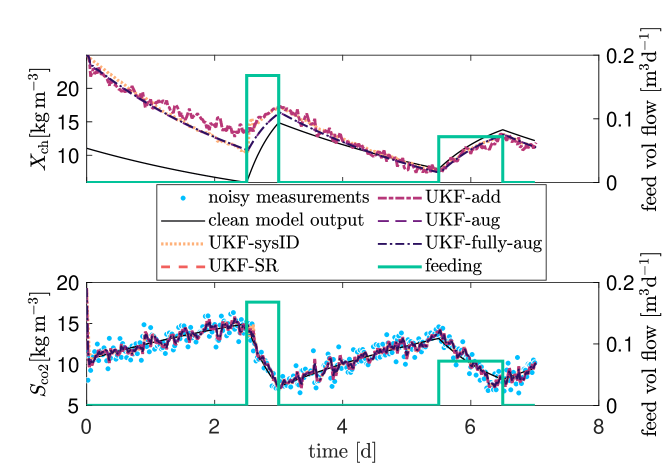
Figure 1: Comparison of state estimation quality through different UKFs with nominal sigma point scaling. Top: Concentration of carbohydrates and corresponding estimations. Bottom: Concentration of dissolved CO₂, measurements and corresponding estimations.

The simulation model (22), (23) contains three measurable and three non-measurable states. However, qualitative filter performance for all measurable and all non-measurable states is largely the same. This holds for all implemented algorithms. Therefore, in the following only one each is shown, which is largely representative of the corresponding two other ones, exceptions are highlighted.

As the non-measurable state, the carbohydrate concentration is chosen for being the largest nutrient fraction. As a measurable state, dissolved carbon dioxide concentration is chosen since it exhibits the largest values and is the easiest one to measure in reality [24].

Smoothing of measurable states, such as dissolved CO₂ in the bottom of Figure 1, is very similar for all UKF versions. This is reinforced through nearly identical values of NRMSE_y, see Table 4. The noise-free output is not met exactly, but the filters clearly smooth the noisy measurements, underlined by low NRMSE_y.

Table 4: Comparison of unconstrained UKF performance with default sigma point scaling ($\gamma=2.4495$) according to (4) and (5).

Algorithm	NRMSExa	NRMSEyb	Run time [s]
UKF-sysID	0.0255	0.0062	1.73
UKF-SR	0.0460	0.0062	2.16
UKF-add	0.0460	0.0062	2.29
UKF-aug	0.0193	0.0050	3.66
UKF-fully-aug	0.0193	0.0058	4.14
aaverage value of all non-measurable states baverage value of all
measurable states

For the non-measurable states, such as carbohydrates in the top of Figure 1, all filters approach the true trajectory despite the initial estimation error. As of $t\approx$4\text{\,}\mathrm{d}$$, estimations agree well with true values. In light of a plant-model mismatch, it is plausible that they do not match exactly.

Yet, convergence behavior of the algorithms differs. UKF-add and UKF-SR deliver identical results, and hence show overlapping graphs and the same NRMSE_x. They both do not involve augmentation, so essentially their flow of algorithmic operations is the same. Their identical performance emphasizes that the square root formulation of the additive UKF derived in [23] is equivalent to the conventional additive UKF. However, both UKF-add and UKF-SR show a slower convergence than UKF-sysID, clearly visible before the first feeding, and reflected in a higher NRMSE_x. Since UKF-sysID and UKF-SR are both based on the square root UKF [25], their graphs should match. However, their discrepancy might be due to different numerical performance. This is likely the case, especially because all three additive UKFs delivered negative state estimates for the lipids concentration ($x_{5}$) before the first feeding. To this end, UKF-add exhibited the lowest estimates of $x_{5}$. Since negative concentrations are beyond the physically meaningful domain of the model, these negative estimates of $x_{5}$ might also influence the other state estimates.

By contrast, the augmented versions UKF-aug and UKF-fully-aug deliver no negative and much less noisy state estimates, see Figure 1. They approach the true trajectory faster and yield a lower NRMSE_x than UKF-sysID, see Table 4. Run times of all additive UKF versions over the entire simulation horizon are in the same range of about $2\text{\,}\mathrm{s}$. Among them, UKF-sysID is the fastest. This is plausible since it is a commercial implementation optimized for numerical efficiency. By comparison, run times of UKF-aug and UKF-fully-aug are clearly higher, reflecting the higher resulting system order, cf. (7) and (8).

5.1.2 Reduced Sigma Point Scaling

For all unconstrained UKF variants, except the benchmark, the sigma point scaling was reduced by changing the scaling factor $\gamma$ from 2.4495 (according to nominal UKF scaling (4)) to 1. The resulting performance is illustrated in Figure 2, with corresponding graphs indicated by the name extension -$\gamma$.

Figure 2: Comparison of state estimation quality through different UKFs with modified sigma point scaling (reduced scaling factor $\gamma=1$). For the benchmark UKF-sysID, conventional tuning was retained for comparison. Top: Concentration of carbohydrates and corresponding estimations. Bottom: Concentration of dissolved CO₂, measurements and corresponding estimations.

Table 5: Comparison of unconstrained UKF performance with modified sigma point scaling ($\gamma=1$).

Algorithm	NRMSExa	NRMSEyb	Run time [s]
UKF-SR-$\gamma$	0.0200	0.0035	2.18
UKF-add-$\gamma$	0.0200	0.0035	2.15
UKF-aug-$\gamma$	0.0198	0.0035	3.84
UKF-fully-aug-$\gamma$	0.0198	0.0056	4.40
aaverage value of all non-measurable states baverage value of all
measurable states

Performance improves especially for the additive variants UKF-add-$\gamma$ and UKF-SR-$\gamma$. This manifests in lower NRMSE values than for nominal scaling and also than UKF-sysID. At the same time, about the same run times are maintained, as illustrated in Tables 4 and 5. Moreover, no negative values for estimated lipids concentrations ($x_{5}$) are obtained anymore.

For the augmented versions, the positive effect of reducing $\gamma$ is not as clear: NRMSE_y reduces for UKF-aug-$\gamma$, whereas NRMSE_x improves only slightly. For the fully augmented version both NRMSE values remain almost unchanged at an acceptable level. We conclude that for the given model and simulation scenario, sigma point scaling according to [15] does not necessarily deliver the best possible estimation performance. This especially holds for the additive noise case.

Note that reducing $\gamma$ does not affect the aggregation step of the scaled unscented transformation, since it is still holds that $\sum_{i}W_{i}^{x}=1$, cf. (6). Moreover, reducing the scaling factor $\gamma$ could also be achieved through negative values of $\kappa$, see (4). However, this affects the parameter $\lambda$ and hence the weights of the mean and covariance. The scaled unscented transformation eventually still remains unchanged, although scaled linearly in $\lambda$. Choosing negative values of $\kappa$ delivered exactly the same results as those obtained with $\kappa=0$. We thus conclude that for the purpose of smoothing noisy measurements, reducing the scaling of sigma points can be beneficial to estimation performance.

5.2 Constrained Case

The algorithms presented so far did not explicitly account for state constraints. [8] suggested to introduce clipping in various locations of the unconstrained UKFs to address state estimates beyond physically meaningful bounds. However, clipping diminished the estimation quality in our case (results not shown). This behavior appears to be reasonable: abrupt clipping without simultaneously adapting the sigma point distribution distorts the unscented transformation. A remedy may lie in applying the truncation method [26] proposed for linear Kalman filters and extending it for UKFs. This was, however, not further pursued here.

By contrast, accounting for state constraints through solving the optimization problem (13a) could be shown to improve estimation performance especially for additive noise, which is explained in the following.

The constrained UKFs were implemented for all three noise scenarios, delivering additive (cUKF-add), augmented (cUKF-aug) and fully augmented cUKFs (cUKF-fully-aug). Note that nominal sigma point scaling (4) was applied. Furthermore, the optimization of each cUKF could be described by either the NLP (14) or the QP formulation (16) since the model output (23) is linear [8]. For the NLP, gradients and the Hessian were either approximated by finite differences (cUKF-NLP); by providing analytic expressions for the gradients (cUKF-NLP-grad); or both gradients and Hessian (cUKF-NLP-grad-hess). All setups of the optimization problems for a given noise scenario delivered the same estimations. Therefore, Figure 3 shows the cUKF performances only with respect to a given noise scenario. Furthermore, Table 6 summarizes corresponding NRMSE values. The stated run times apply for the NLP setup with finite differences.

The measurable states are smoothed comparably well as for the unconstrained UKFs, mirrored by NRMSE_y values in between nominal and reduced sigma point scaling, cf. Tables 4, 5 and 6. For this reason, the graphs of CO₂ measurements and smoothed estimates are not shown here again.

Table 6: Comparison of constrained UKF performance. Run times apply for NLP formulation without gradients and Hessian.

Algorithm	NRMSExa	NRMSEyb	Run time [s]
cUKF-add	0.0155	0.0056	54.17
cUKF-aug	0.0364	0.0048	129.57
cUKF-fully-aug	0.0342	0.0045	158.06
aaverage value of all non-measurable states baverage value of all
measurable states

Instead, Figure 3 illustrates estimation performance for the (non-measurable) carbohydrates and lipids concentrations $X_{\mathrm{ch}}$ and $X_{\mathrm{li}}$. The latter exhibited negative values for all additive, unconstrained UKFs with nominal values of $\gamma$, see Section 5.1.1.

Figure 3: Comparison of state estimation quality through different constrained UKFs. Top: Concentration of carbohydrates and corresponding estimations. Bottom: Concentration of lipids and corresponding estimations.

It is clear that for carbohydrates, estimates of all three algorithms do not differ much, and they all approach the true trajectory well. This is reflected in very similar values of NRMSE_x for carbohydrates between 0.024 and 0.029. The augmented versions cUKF-aug and cUKF-fully-aug are slightly closer to the true value than cUKF-add.

By contrast, the lipids estimations differ significantly, Figure 3 bottom. This might, on the one hand, be attributed to the lower order of magnitude of $X_{\mathrm{li}}$. [9] mentioned that for estimates close to the constraints (i.e. very low concentrations in our case), the optimization might result in a biased estimate. On the other hand, closely inspecting the algorithms of cUKF-aug and cUKF-fully-aug reveals a crucial aspect not addressed in [8]. Therein the authors adopt the NLP from [9] and apply it to the augmented cases, while in [9] it was formulated for the additive noise case. To this end, it remains unclear how cUKF-aug and cUKF-fully-aug effectively differ from each other aside from the augmentation, since the intermediate steps for computing the estimated output $\hat{y}$ and the corresponding covariance matrix $P_{y_{k}y_{k}}$ do not come into effect in the constrained case. Instead, the outputs resulting from the updated sigma points $h(\chi_{k,i}^{x})$ are computed in each iteration of the optimization, (14). Additionally, [8] apply the nominal output $h(x_{k})$ in the cost function of the fully augmented noise case, neglecting the non-additive formulation $h(x_{k},v_{k})$ used in the unconstrained UKFs.

We thus conclude that the NLP formulation (14) might only deliver reliable state estimates for the additive noise case (cUKF-add) for which it was originally proposed, especially for state estimates close to the bounds. This may also explain why the graphs of cUKF-aug and cUKF-fully-aug both show similarly poor lipids estimates in Figure 3. The poor estimates of $X_{\mathrm{li}}$ through cUKF-aug and cUKF-fully-aug also dominate the comparably high values of NRMSE_x in Table 6.

Estimation results of all optimization setups for a given noise scenario are identical. This emphasizes that for linear output equations the QP reformulation of the NLP by [8] is indeed equivalent, and that the provision of gradients and Hessian increases numerical efficiency without jeopardizing accuracy.

Run times of the constrained UKFs are generally higher than for the unconstrained versions. However, they can be vastly reduced through a) analytic expressions of gradient and Hessian for the NLP, and b) through the QP formulation in case of linear outputs, as illustrated in Figure 4. Given the higher resulting system order caused by augmentation, it is plausible that numerical effort for cUKF-aug and cUKF-fully-aug is higher than for cUKF-add.

The reduced run times of the improved NLP setups can be explained when considering the average number of iterations and cost function calls before convergence, summarized in Table 7. By default, fmincon solves the NLP with an interior-point algorithm which involves to approximate gradient and Hessian of the cost function through finite differences [21]. For this purpose, the cost function during one iteration of optimization needs to be computed multiple times. In contrast, approximation through finite differences becomes redundant with analytic expressions of gradients and Hessian. In case only the gradients are provided, the number of iterations remains the same but the number of cost function calls drops from 104 to 19. Moreover, additionally providing the Hessian reduces the number of iterations from 14 to 5, and consequently further diminishes the number of cost function calls from 19 to 6. For cUKF-QP, the solver quadprog makes use of algorithms optimized for QPs and thus required even fewer iterations.

Table 7: Comparison of optimization performance of cUKF-add for different optimization setups.

Algorithm	# Function callsa	# Iterationsb
cUKF-add-NLP	104	13
cUKF-add-NLP-grad	19	14
cUKF-add-NLP-grad-hess	6	5
cUKF-add-QP	-	4
amedian of function calls bmedian of iterations

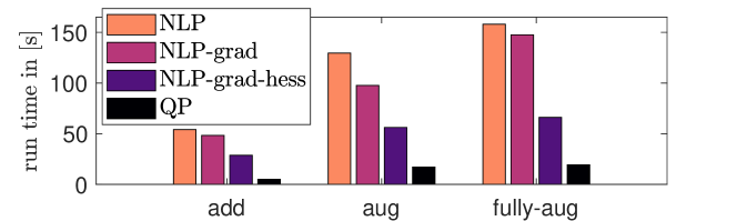
Figure 4: Run times of cUKF versions with all three noise cases in different optimization setups.

5.3 Summary

Figure 5 compares the best versions of the different classes of implemented algorithms with respect to run time and estimation accuracy, expressed as the average NRMSE over both measurable and non-measurable states.

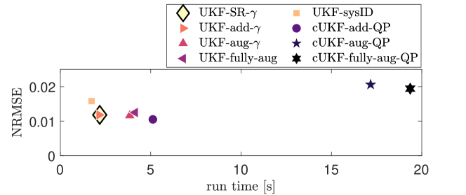
Figure 5: Comparison of best-in-class implementations of UKFs by means of run time and estimation error.

The unconstrained UKFs showed faster run times than the constrained UKFs. The best accuracy was achieved with cUKF-add. However, the unconstrained UKFs UKF-aug-$\gamma$ as well as the equivalent UKF-add-$\gamma$ and UKF-SR-$\gamma$ deliver almost the same accuracy with lower run times. Among the constrained UKFs, the augmented cUKF versions cUKF-aug and cUKF-fully-aug could not compete with the additive variant cUKF-add with respect to both run time and accuracy.

6 Conclusion

This study examined various UKF implementations and applied them to a simplified AD model. Crucial details of the underlying algorithms as well as modifications to leverage improved numerical performance were addressed. This provides useful hints for practitioners working with Kalman filters.

The best estimation accuracy was achieved with cUKF-add. The QP reformulation of the underlying NLP massively reduced the run time without compromising estimation accuracy. However, it is only applicable for models with linear output equations. For models involving nonlinear output equations, cUKF-NLP-add-grad-hess presents a useful alternative although the associated run time is much higher, see Figure 4.

If run time is critical, the unconstrained variants UKF-SR-$\gamma$, UKF-add-$\gamma$ and UKF-aug-$\gamma$ with reduced sigma point scaling represent competitive alternatives. The most convenient implementations might be the augmented unconstrained UKF-aug and UKF-fully-aug, which deliver acceptable estimations at low run times, even for nominal sigma point scaling.

Lastly, the present study was limited to simulation data and a reduced AD model with linear outputs. In future studies, the presented UKFs must therefore be applied to real measurement data and higher-order AD models involving nonlinear output equations such as those proposed by [10] or [27].

Appendix: Model Equations

In the following, the system equations of the model used in the present study are derived, cf. Section 4. Since it represents a vastly simplified form of the ADM1-R4 proposed by Weinrich and Nelles (2021) [10], it is called ADM1-R4-Core. It describes the degradation of macro nutrients (carbohydrates, proteins and lipids) directly to biogas, i.e. methane (CH₄) and carbon dioxide (CO₂), with the help of microbial biomass.

Compared with the ADM1-R4, the following simplifications were made:

• Inorganic nitrogen $S_{\mathrm{IN}}$ was omitted because it acts as a quasi-autonomous state as described in [14]. This means that its dynamics are only affected by other states, but inorganic nitrogen itself has no effect on the other states. Therefore, it can be deleted from the differential equation system without changing the dynamics of the remaining system.

• The same holds for the ash concentration $X_{\mathrm{ash}}$ which was only added in [14] to represent total and volatile solids measurements.

• The gas phase was entirely omitted for two reasons: First, this results in linear output equations. Second, this allows to drop two additional states ($S_{\mathrm{ch4,gas}}$ and $S_{\mathrm{co2,gas}}$).

• The mass concentrations of dissolved CH₄ and CO₂ as well as microbial biomass were assumed to be directly measurable.

The state vector is comprised of the six mass concentrations

$$x=\left[S_{\mathrm{ch4}},S_{\mathrm{co2}},X_{\mathrm{ch}},X_{\mathrm{pr}},X_{\mathrm{li}},X_{\mathrm{bac}}\right]^{T}.$$ (30)

The differential equations of ADM1-R4-Core read as follows

$$\dot{x}_{1} =c_{1}\left(\xi_{1}-x_{1}\right)u+a_{11}c_{2}x_{3}+a_{12}c_{3}x_{4}+a_{13}c_{4}x_{5},$$ (31a)

$$\dot{x}_{2} =c_{1}\left(\xi_{2}-x_{2}\right)u+a_{21}c_{2}x_{3}+a_{22}c_{3}x_{4}+a_{23}c_{4}x_{5},$$ (31b)

$$\dot{x}_{3} =c_{1}\left(\xi_{3}-x_{3}\right)u-c_{2}x_{3}+a_{34}c_{5}x_{6},$$ (31c)

$$\dot{x}_{4} =c_{1}\left(\xi_{4}-x_{4}\right)u-c_{3}x_{4}+a_{44}c_{5}x_{6},$$ (31d)

$$\dot{x}_{5} =c_{1}\left(\xi_{5}-x_{5}\right)u-c_{4}x_{5}+a_{54}c_{5}x_{6},$$ (31e)

$$\dot{x}_{6} =c_{1}\left(\xi_{6}-x_{6}\right)u+a_{61}c_{2}x_{3}+a_{62}c_{3}x_{4}+a_{63}c_{4}x_{5}-c_{5}x_{6}.$$ (31f)

The measurement equations reduce to

$$y_{1} =S_{\mathrm{ch4}}=x_{1},$$ (32a)

$$y_{2} =S_{\mathrm{co2}}=x_{2},$$ (32b)

$$y_{3} =X_{\mathrm{bac}}=x_{6},$$ (32c)

which can be put in vector-matrix form

$$y=\begin{bmatrix}y_{1}\\ y_{2}\\ y_{3}\end{bmatrix}=\begin{bmatrix}S_{\mathrm{ch4}}\\ S_{\mathrm{co2}}\\ X_{\mathrm{bac}}\end{bmatrix}=\begin{bmatrix}x_{1}\\ x_{2}\\ x_{6}\end{bmatrix}=\begin{bmatrix}1&0&0&0&0&0\\ 0&1&0&0&0&0\\ 0&0&0&0&0&1\end{bmatrix}\,x.$$ (33)

Therein, $a_{ij}$ are the absolute values of the entries of the petersen matrix given in Tab. 8, where $i$ denotes the column (component) and $j$ the row (process). For brevity, only those entries with an absolute value $\neq 1$ or $\neq 0$ were denoted with $a_{ij}$ specifically.

Table 8: Petersen matrix of ADM1-R4-Core, derived from [28].

Component i $\rightarrow$		1	2	3	4	5	6
j	Process $\downarrow$	$S_{\mathrm{ch4}}$	$S_{\mathrm{co2}}$	$X_{\mathrm{ch}}$	$X_{\mathrm{pr}}$	$X_{\mathrm{li}}$	$X_{\mathrm{bac}}$	Process rate $r_{j}$
1	Fermentation $X_{\mathrm{ch}}$	0.2482	0.6809	-1			0.1372	$c_{2}\,x_{3}$
2	Fermentation $X_{\mathrm{pr}}$	0.3221	0.7954		-1		0.1723	$c_{3}\,x_{4}$
3	Fermentation $X_{\mathrm{li}}$	0.6393	0.5817			-1	0.2286	$c_{4}\,x_{5}$
[0.6pt/1.8pt]
4	Decay $X_{\mathrm{bac}}$			0.18	0.77	0.05	-1	$c_{5}\,x_{6}$

Table 9 summarizes the model parameters $c_{i}$ of ADM1-R4-Core as well as the control variable. The dotted horizontal line should underline the different categories of parameters. $c_{1}$ is time invariant, whereas $c_{2}$ - $c_{5}$ are slowly time variant for varying substrates and subsequently adapting composition of the microbial community. During long-term process operation in practice, $c_{2}$ - $c_{5}$ need to be repeatedly updated throug parameter identification.

Table 9: Model parameters and control variable of ADM1-R4-Core according to Weinrich and Nelles (2021) [10] and in standard control notation. The stated true values apply for creation of synthetic measurement data and were taken from [29]. By contrast, the UKF values were used for Kalman filtering and were chosen differently to account for a plant model mismatch, see Section 4.1.

Control notation	Notation according to [10]	True value	UKF value
$u$	$q$	see Table 1
$c_{1}$	$V_{\mathrm{liq}}^{-1}$	$0.01\text{\,}{\mathrm{L}}^{-1}$
[0.6pt/1.8pt]
$c_{2}$	$k_{\mathrm{ch}}$	$0.25\text{\,}{\mathrm{h}}^{-1}$	$0.3196\text{\,}{\mathrm{h}}^{-1}$
$c_{3}$	$k_{\mathrm{pr}}$	$0.20\text{\,}{\mathrm{h}}^{-1}$	$0.2557\text{\,}{\mathrm{h}}^{-1}$
$c_{4}$	$k_{\mathrm{li}}$	$0.10\text{\,}{\mathrm{h}}^{-1}$	$0.1278\text{\,}{\mathrm{h}}^{-1}$
$c_{5}$	$k_{\mathrm{dec}}$	$0.02\text{\,}{\mathrm{h}}^{-1}$	$0.0256\text{\,}{\mathrm{h}}^{-1}$

In (31), $\xi_{i}$ denote the inlet concentrations of inflowing substrates. For the scope of this study, a mixture of cattle manure and maize silage was assumed as a substrate. The corresponding inlet concentrations were taken from [29] and are shown in Table 10.

Table 10: Inlet concentrations $\xi_{i}$ for substrate mix of cattle manure and maize silage taken from [29].

Variable	Corresponding component	Value [$\mathrm{kg}\text{\,}{\mathrm{m}}^{-3}$]
$\xi_{1}$	$S_{\mathrm{ch4}}$	$0$
$\xi_{2}$	$S_{\mathrm{co2}}$	$0$
$\xi_{3}$	$X_{\mathrm{ch}}$	$23.398$
$\xi_{4}$	$X_{\mathrm{pr}}$	$4.750$
$\xi_{5}$	$X_{\mathrm{li}}$	$1.381$
$\xi_{6}$	$X_{\mathrm{bac}}$	$0$

Lastly, measurement noise was considered by adding zero-mean Gaussian random numbers to nominal outputs obtained through (32). Corresponding standard deviations were chosen as summarized in Table 11.

Table 11: Standard deviations of additive measurement noise of individual measurements.

Variable	Corresponding output	Value [$\mathrm{kg}\text{\,}{\mathrm{m}}^{-3}$]
$\sigma_{1}$	$y_{1}=S_{\mathrm{ch4}}$	$0.8$
$\sigma_{2}$	$y_{2}=S_{\mathrm{co2}}$	$1.0$
$\sigma_{3}$	$y_{3}=X_{\mathrm{bac}}$	$0.4$

References

- [1] Susanne Theuerl, Christiane Herrmann, Monika Heiermann, Philipp Grundmann, Niels Landwehr, Ulrich Kreidenweis, and Annette Prochnow. The future agricultural biogas plant in germany: A vision. Energies, 12(3):396, 2019.
- [2] Pezhman Kazemi, Jean-Philippe Steyer, Christophe Bengoa, Josep Font, and Jaume Giralt. Robust data-driven soft sensors for online monitoring of volatile fatty acids in anaerobic digestion processes. Processes, 8(1):67, 2020.
- [3] Maik Gentsch and Rudibert King. Real-time estimation of parameter maps. IFAC-PapersOnLine, 53(2):2391–2396, 2020.
- [4] Junbo Zhao and Lamine Mili. A decentralized h-infinity unscented kalman filter for dynamic state estimation against uncertainties. IEEE Transactions on Smart Grid, 10(5):4870–4880, 2019.
- [5] Niloofar Raeyatdoost, Michael Bongards, Thomas Bäck, and Christian Wolf. Robust state estimation of the anaerobic digestion process for municipal organic waste using an unscented kalman filter. Journal of Process Control, 121(1):50–59, 2023.
- [6] Annina Kemmer, Nico Fischer, Terrance Wilms, Linda Cai, Sebastian Groß, Rudibert King, Peter Neubauer, and M. Nicolas Cruz Bournazou. Nonlinear state estimation as tool for online monitoring and adaptive feed in high throughput cultivations. Biotechnology and Bioengineering, 120(11):3261–3275, 2023.
- [7] Andrea Tuveri, Fernando Pérez-García, Pedro A. Lira-Parada, Lars Imsland, and Nadav Bar. Sensor fusion based on extended and unscented kalman filter for bioprocess monitoring. Journal of Process Control, 106:195–207, 2021.
- [8] S. Kolås, B. A. Foss, and T. S. Schei. Constrained nonlinear state estimation based on the ukf approach. Computers & Chemical Engineering, 33(8):1386–1401, 2009.
- [9] Pramod Vachhani, Shankar Narasimhan, and Raghunathan Rengaswamy. Robust and reliable estimation via unscented recursive nonlinear dynamic data reconciliation. Journal of Process Control, 16(10):1075–1086, 2006.
- [10] Sören Weinrich and Michael Nelles. Systematic simplification of the anaerobic digestion model no. 1 (ADM1) - model development and stoichiometric analysis: Application. Bioresource technology, 333:125124, 2021.
- [11] D. J. Batstone, J. Keller, I. Angelidaki, S. V. Kalyuzhnyi, S. G. Pavlostathis, A. Rozzi, W.T.M. Sanders, H. Siegrist, and V. A. Vavilin. The IWA Anaerobic Digestion Model No 1 (ADM1). Water science and technology: a journal of the International Association on Water Pollution Research, 45(10):65–73, 2002.
- [12] Sören Weinrich, Eric Mauky, Thomas Schmidt, Christian Krebs, Jan Liebetrau, and Michael Nelles. Systematic simplification of the anaerobic digestion model no. 1 (ADM1) - laboratory experiments and model application. Bioresource technology, 333:125104, 2021.
- [13] Eric Mauky, Sören Weinrich, Hans-Joachim Nägele, H. Fabian Jacobi, Jan Liebetrau, and Michael Nelles. Model predictive control for demand-driven biogas production in full scale. Chemical Engineering & Technology, 39(4):652–664, 2016.
- [14] Simon Hellmann, Arne-Jens Hempel, Stefan Streif, and Sören Weinrich. Observability and identifiability analyses of process models for agricultural anaerobic digestion plants. In 2023 24th International Conference on Process Control (PC), pages 84–89. IEEE, 2023.
- [15] Rudolph van der Merwe and Eric Wan. Sigma-point kalman filters for integrated navigation. Proceedings of the 60th Annual Meeting of the Institute of Navigation, 2004.
- [16] Dan Simon and Donald L. Simon. Aircraft turbofan engine health estimation using constrained kalman filtering. Journal of Engineering for Gas Turbines and Power, 127(2):323–328, 2005.
- [17] The MathWorks, Inc. Matlab version 9.13.0 (r2022b), 2022.
- [18] Steven A. Holmes, Georg Klein, and David W. Murray. An square root unscented kalman filter for visual simultaneous localization and mapping. IEEE transactions on pattern analysis and machine intelligence, 31(7):1251–1263, 2009.
- [19] Jouni Hartikainen, Arno Solin, and Simo Särkkä. EFK/UKF Toolbox For Matlab. Github repository: https://github.com/eea-sensors/ekfukf, last visited 10/24, 2020.
- [20] Francesco de Vivo, Alberto Brandl, Manuela Battipede, and Piero Gili. Joseph covariance formula adaptation to square-root sigma-point kalman filters. Nonlinear Dynamics, 88(3):1969–1986, 2017.
- [21] The MathWorks, Inc. Writing Scalar Objective Functions. Matlab documentation: https://www.mathworks.com/help/optim/ug/writing-scalar-objective-functions.html, last visited 10/24, 2023.
- [22] René Schneider and Christos Georgakis. How to not make the extended kalman filter fail. Industrial & Engineering Chemistry Research, 52(9):3354–3362, 2013.
- [23] Rudolph van der Merwe and Eric. Wan. The square-root unscented kalman filter for state and parameter-estimation. In 2001 IEEE International Conference on Acoustics, Speech, and Signal Processing. Proceedings (Cat. No.01CH37221), pages 3461–3464. IEEE, 2001.
- [24] Flavia Neddermeyer, Niko Rossner, and Rudibert King. Model-based control to maximise biomass and phb in the autotrophic cultivation of ralstonia eutropha. IFAC-PapersOnLine, 48(8):1100–1107, 2015.
- [25] The MathWorks, Inc. Extended and Unscented Kalman Filter Algorithms for Online State Estimation. Matlab documentation: https://www.mathworks.com/help/control/ug/extended-and-unscented-kalman-filter-algorithms-for-online-state-estimation.html#bvf4mkl, last visited 10/24, 2023.
- [26] Dan Simon and Donald L. Simon. Constrained kalman filtering via density function truncation for turbofan engine health estimation. International Journal of Systems Science, 41(2):159–171, 2010.
- [27] O. Bernard, Z. Hadj-Sadok, D. Dochain, A. Genovesi, and J. P. Steyer. Dynamical model development and parameter identification for an anaerobic wastewater treatment process. Biotechnology and Bioengineering, 75(4):424–438, 2001.
- [28] Sören Weinrich. Praxisnahe Modellierung von Biogasanlagen: Systematische Vereinfachung des Anaerobic Digestion Model No. 1 (ADM1). PhD thesis, Universität Rostock, 2017.
- [29] Sören Weinrich. ADM1. Github repository: https://github.com/soerenweinrich/adm1, last visited 10/24, 2021.