Improving Robustness and Reliability in Medical Image Classification with Latent-Guided Diffusion and Nested-Ensembles

Abstract

While deep learning models have achieved remarkable success across a range of medical image analysis tasks, deployment of these models in real clinical contexts requires that they be robust to variability in the acquired images. While many methods apply predefined transformations to augment the training data to enhance test-time robustness, these transformations may not ensure the model’s robustness to the diverse variability seen in patient images. In this paper, we introduce a novel three-stage approach based on transformers coupled with conditional diffusion models, with the goal of improving model robustness to the kinds of imaging variability commonly encountered in practice without the need for pre-determined data augmentation strategies. To this end, multiple image encoders first learn hierarchical feature representations to build discriminative latent spaces. Next, a reverse diffusion process, guided by the latent code, acts on an informative prior and proposes prediction candidates in a generative manner. Finally, several prediction candidates are aggregated in a bi-level aggregation protocol to produce the final output. Through extensive experiments on medical imaging benchmark datasets, we show that our method improves upon state-of-the-art methods in terms of robustness and confidence calibration. Additionally, we introduce a strategy to quantify the prediction uncertainty at the instance level, increasing their trustworthiness to clinicians using them in clinical practice.

I Introduction

In the rapidly evolving domain of medical imaging analysis, deep learning has emerged as a cornerstone for diagnostic advancements [1, 2, 3, 4, 5, 6, 7, 8, 9], notably in tasks such as detection of diabetic retinopathy in eye fundus images [2], classification of skin cancer [1], and identification of cancerous regions in mammograms [7]. While these approaches have achieved unprecedented success in controlled settings, their real-world applications reveal significant performance degradation in terms of inaccurate predictions and poorly calibrated confidence, thus leading to untrustworthy results in clinical settings [10, 11]. This is often attributed to differences in images structure (Fig. 1) arising from varying physical parameters of medical imaging sensors. Formally speaking, this is due to differences between the training data distribution and the actual test data distribution, and this discrepancy is usually unknown. Deep learning methods, while powerful, exhibit sensitivity to discrepancies between training and test distributions, especially in the realm of medical imaging [12]. The real-world nature of medical data collection, with its inherent variability, poses challenges that conventional models struggle to address. A limited body of existing research has applied known transformations, such as rotations and translations, during training [13]. However, these contrived augmentations might not accurately represent the real-world changes encountered during clinical deployments. Variations in image quality at test-time, often arising from differing imaging devices and settings, have not been extensively addressed [14].

This this work, we introduce a novel framework for medical image classification that inherently copes with these discrepancies. Our approach leverages the robustness of transformer encoder blocks in order to extract consistent representations across diverse image presentations. Our model then employed a novel diffusion process, informed by a prior, in order to generate more accurate and robust predictions. The robustness of our predictions is then bostered by additionally integrating a unique ensemble technique named Nested-ensemle, which produces sets of predictions and utlizes bi-level aggregation functions to improve accuracy and uncertainty estimates.

Extensive experiments performed on the Tuberculosis chest X-ray classification benchmark [15] and the subset of ISIC skin caner classification benchmark [16], indicate the superiority of the proposed method, in terms of accuracy and the expected calibration error metrics. We show particular performance gains across diverse experimental settings, which are simulated by substantially varying image presentations, plus additional experiments on adversarial attacks. Finally, we provide a strategy to estimate, and an in-depth analysis of the performances, the model confidences and prediction uncertainties.

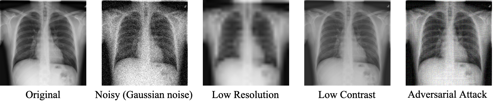
Figure 1: Sample images of the Tuberculosis chest X-ray dataset under different transformations: noisy, low resolution, low contrast, as well as a sample image of the applied adversarial attack.

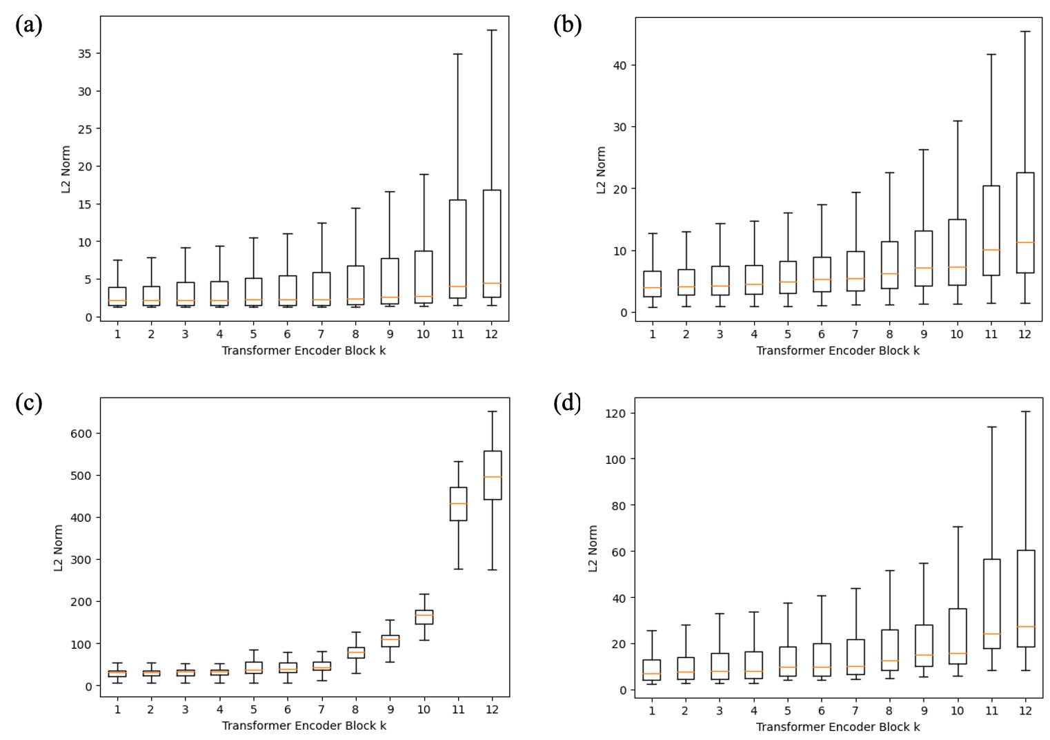
Figure 2: The Euclidean distance between the token sequence of image variants (under a range of conditions) and its original copy increases as going deeper into the encoder block hierarchy under (a) noisy , (b) lower-resolution , (c) lower-contrast contexts , and (d) adversarial attack.

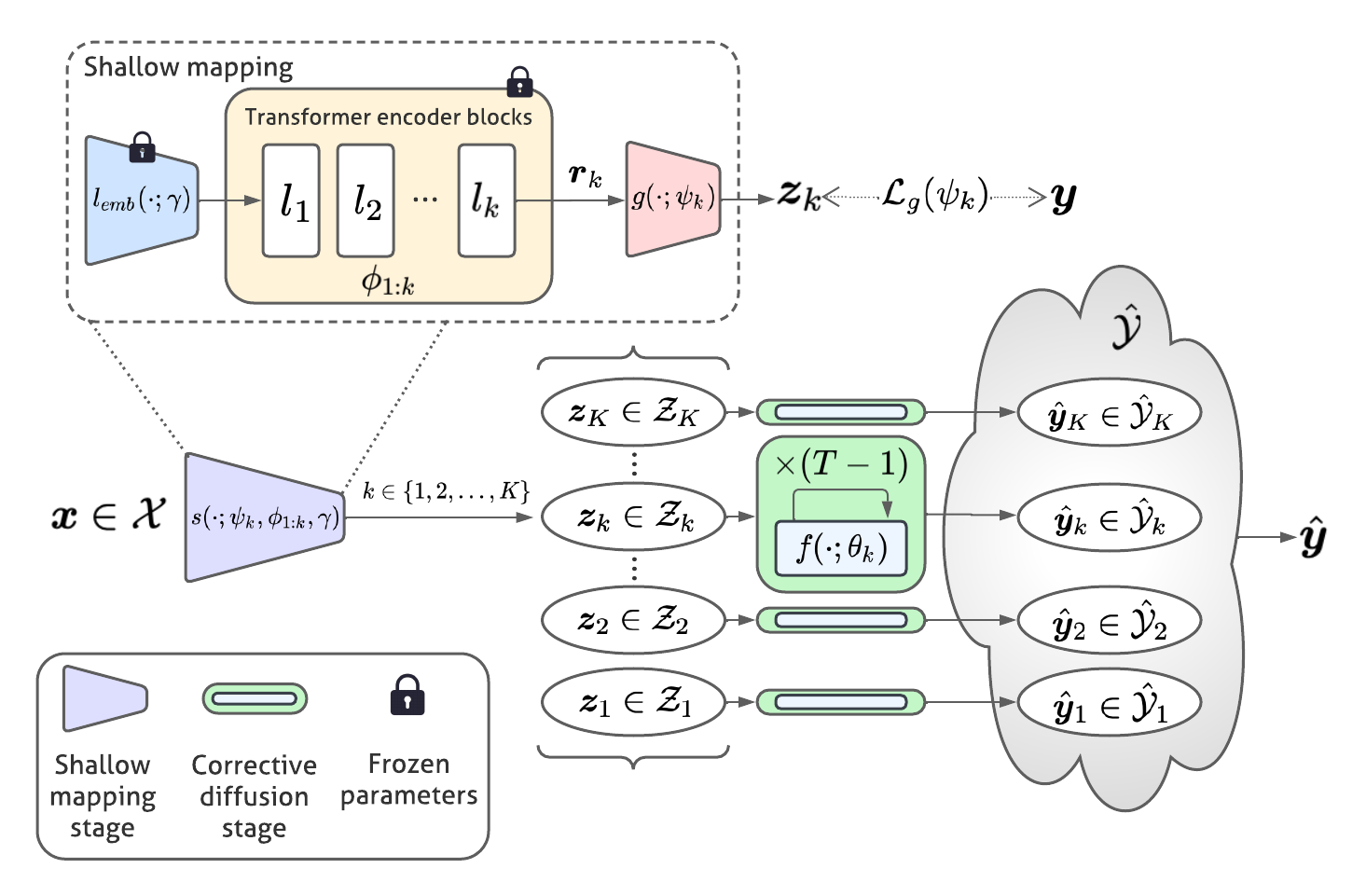
Figure 3: An illustration of the proposed 3-stage method: (1) shallow mapping stage, (2) corrective diffusion stage, (3) prediction aggregation. Parameters of the backbone image classification model are frozen during the training of the remaining components.

II Related Work

Recent advancements in robust medical image classification have been significantly propelled by deep neural networks. Xue et al. [17] emphasize the challenges posed by the reliance on expert annotations in the medical field and introduces a collaborative training paradigm to handle noisy-labeled images, demonstrating enhanced performance across various noise types. Manzari et al. [18], echoing concerns about the susceptibility of Convolutional Neural Networks (CNNs) to adversarial attacks, propose a CNN-transformer hybrid model which offers improved robustness in medical image classification. Almalik et al. [19] highlights the vulnerability of Vision Transformers (ViTs) to adversarial attacks and present a robust architecture leveraging initial block feature for medical image classfication. Dash et al. [20] pivot the focus to dataset quality, suggesting the integration of illumination normalization techniques with CNNs to boost classification accuracy. These studies collectively emphasize the importance of robustness and data quality in medical image classification.

Diffusion-based or score-based deep generative models have notably emerged as a potent methodology for high-dimensional data distribution modeling [21, 22]. These models consist of two main processes: a forward process $\mathbf{q}$, that methodically eliminates structure from the data $\bm{x}$ by introducing noise, and a generative model $\mathbf{p}$ (or reverse process), that carefully reintroduces structure, commencing from noise $\bm{\epsilon}_{t}$. Typically, the forward process involves a Gaussian distribution that seamlessly shifts from a less noisy latent state at a given timestep $t$ to a more noisy latent state at the subsequent timestep. Latent diffusion models [23] convert the diffusion process to the latent space instead of the original data space, reducing computational cost while obtaining better data feature representations for sampling data that conditioned on multimodal information.

Taking inspiration from the success of diffusion models in general image generation, the medical imaging domain has started to explore its capabilities. For instance, recent work introduced a sequence-aware diffusion model tailored for the generation of longitudinal medical images [24]. It leverages sequential features extracted from a transformer module as the conditional information in a diffusion model to learn longitudinal dependencies, even in cases with missing data during training. Furthermore, another innovative endeavor utilizes the diffusion probabilistic model for medical image segmentation tasks [25]. By integrating dynamic conditional encoding and a filter that removes noisy features in the Fourier space, it offers enhanced step-wise regional attention and effectively mitigates the adverse effects of high-frequency noise components.

Generative models have attracted the attention of many researchers in image classification [26, 27, 28]. Among these works, Han et al. [28] proposed Classification And Regression Diffusion models, a class of models that tackles supervised learning problems with a conditional generation model. It blends a denoising diffusion-based conditional generative model with a pre-trained conditional mean estimator to predict $p(\bm{y}\mid\bm{x})$ precisely. The approach treats each one-hot label $\bm{y}$ as a class prototype rather than assuming it is drawn from a categorical distribution. This adaptation to a continuous data and state space allows the preservation of the Gaussian diffusion model framework [22].

III Method

We aim to establish a generalized, robust deep learning model tailored for medical image classification. We have devised an image encoder designed to learn representations invariant to input distribution shifts. Following this, we introduce a diffusion-based generative model that takes into account the representation variance produced by the encoder, effectively mitigating the degradation in prediction performance due to out-of-distribution inputs. Further, we employ a deep ensemble of multiple models to achieve more reliable outcomes. In essence, our approach comprises three pivotal components: (i) the image encoding procedure, termed the shallow mapping stage, (ii) the diffusion process, denominated as the corrective diffusion stage, and (iii) the prediction aggregation stage designed specifically for our bi-level ensemble. The overall system design is illustrated in Fig. 3.

III-A The shallow mapping stage

We formulate our objective to minimize the impact of test-time input distribution shift on prediction outcomes, aiming to enhance the model’s generalization capabilities. Inspired by the work of Almalik et al. [19] on robust learning in adversarial samples, we further discern that models based on the transformer [29] architecture for visual tasks can aid in acquiring consistent feature representations, even when subjected to out-of-distribution data. In Fig. 2, it is evident that as $k$ increases, the current block’s output becomes more sensitive to input changes. This suggests that blocks closer to the input (shallow blocks) learn more consistent feature representations, despite significant variations in the input. Additionally, we desire the learned feature representations to exhibit consistency and encompass discriminative information of each input instance, which aids the classification task.

In our method, we consider a backbone model consisting of $L$ transformer encoder blocks (Fig. 4), which form a sequence of layers $\{l_{1},l_{2},\dotsc,l_{L}\}$ with a parameter set $\Phi=\{\phi_{k}\}_{k=1}^{L}$. Each layer serves as a function $l_{k}:\mathbb{R}^{(N+1)\times D}\rightarrow\mathbb{R}^{(N+1)\times D}$ with its parameter $\phi_{k}$ that captures the dependencies within current input tokens, and transforms them to inputs to the next layer $l_{k+1}$. Here, $N+1$ denotes the length of token sequence, and $D$ is the embedding size. To fit the image input to a transformer architecture, we follow the patch embedding and position encoding introduced by Dosovitskiy et al. [30], and we denote these two operations as a single embedding function $l_{emb}(\cdot;\gamma)$. Assuming an image input $\bm{x}\in\mathbb{R}^{H\times W\times A}$, here $(H,W)$ is the image resolution, and $A$ is the number of channels. $l_{emb}(\bm{x};\gamma)$ separates the image input $\bm{x}$ into $N$ flattened patches $\bm{x}_{p}\in\mathbb{R}^{N\times(P^{2}\cdot C)}$, here, $(P,P)$ is the resolution of a single patch. It forms a new token sequence $\bm{e}_{0}\in\mathbb{R}^{(N+1)\times D}$ with a linear projection, an extra class token head, and the position encoding. We formulate the calculation in the $k^{\mathrm{th}}$ layer $l_{k}(\cdot;\phi_{k})$ of the backbone model in Eq. 1 with multi-head self-attention (MSA), layer norm (LN), and a fully-connected neural network (MLP). To obtain the prediction of the backbone model, we create $h(\cdot;\omega)$ that takes the first token of $\bm{e}_{L}$ to make classification as shown in Eq. 6. However, it is crucial to clarify that the classification predictions $\hat{\bm{y}}_{b}$ emanating from this backbone model do not directly translate to the final predictions in our approach.

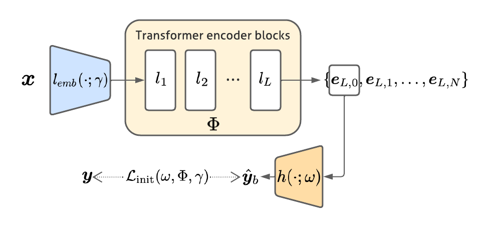
Figure 4: An illustration of the backbone image recognition model based on transformer architecture. It consists of an embedding layer $l_{emb}(\cdot;\gamma)$ that transform 2D images $\bm{x}$ into token sequences, and $L$ transformer encoder blocks to extract hierarchical features, together with a classifier $h(\cdot;\omega)$ that produce a classification prediction $\hat{\bm{y}}_{b}$ based on the classification head token $\bm{e}_{L,0}$. Here $\mathcal{L}_{\mathrm{init}}$ compares $\hat{\bm{y}}_{b}$ with the ground-truth $\bm{y}$.

$$\bm{e}_{k} =l_{k}(\bm{e}_{k-1};\phi_{k})$$ (1)

$$={\rm MLP}({\rm LN}(\bm{e}^{\prime}_{k}))+\bm{e}^{\prime}_{k},$$ (2)

$$\bm{e}^{\prime}_{k} ={\rm MSA}({\rm LN}(\bm{e}_{k-1}))+\bm{e}_{k-1}.$$ (3)

$$\bm{e}_{0} =l_{emb}(\bm{x};\gamma),$$ (4)

$$\bm{e}_{L} =(l_{L}\circ l_{L-1}\circ\dotsc\circ l_{1})(\bm{e}_{0};\Phi),$$ (5)

$$\hat{\bm{y}}_{b} =h(\bm{e}_{L,0};\omega).$$ (6)

In order to attain consistent representations, we engage the first $K$ layers $\{l_{1},l_{2},\dots,l_{K}\}$ of the backbone model, where $K<L$. This results in consistent representations denoted as $\{\bm{r}_{k}\}_{k=1}^{K}$, where $\bm{r}_{k}$ is the output $\bm{e}_{k}$ of the layer $l_{k}$ excluding the head token $\bm{e}_{k,0}$. Explicitly, $\bm{r}_{k}=\{\bm{e}_{k,1},\bm{e}_{k,2},\dots,\bm{e}_{k,N}\}$. For each specific layer level denoted by $k$ within the set $\{1,2,\dots,K\}$, we define a function parameterized by $\psi_{k}$, expressed as $g(\cdot;\psi_{k})$, which is designed to map the representation $\bm{r}_{k}$ to a designated latent space, $\mathcal{Z}_{k}$. We coin this transformation as a shallow mapping. This mapping strategically employs the representation from the shallower layers and transposes it into a space of reduced dimensionality. The formal depiction of the shallow mapping stage is articulated in Eq. 7, where $\bm{z}_{k}$ is an element of $\mathcal{Z}_{k}$. In the interest of conciseness, the shallow mapping for the $k^{\text{th}}$ layer is encapsulated as a singular function $s:\mathcal{X}\rightarrow\mathcal{Z}_{k}$, directly intervening in the image input domain $\mathcal{X}$ to extract consistent representations as shown in Eq. 8.

$$\bm{z}_{k} =g(\bm{r}_{k};\psi_{k})$$ (7)

$$=s(\bm{x};\psi_{k},\phi_{1:k},\gamma).$$ (8)

Properly defining the latent space $Z_{k}$ can be a complex task. The goal here is to ensure that this space not only leverages the strengths of the consistent representation $\bm{r}_{k}$ but is also imbued with discriminative information crucial for the classification task. To this end, we propose a simple yet effective strategy: the space $Z_{k}\subseteq\mathbb{R}^{C}$ is defined as a set of intermediate classification predictions based purely on $\bm{r}_{k}$, where $C$ is the number of classes. Note that these intermediate predictions have more stability to input variances due to the consistent representation $\bm{r}_{k}$ being a constraining factor. In addition, they provide information essential for predicting the class.

III-B The corrective diffusion stage with informative priors

At this stage, we design a corrective diffusion process to refine the intermediate predictions made by the shallow mapping stage. In Sec. III-A, for each $k$ in $\{1,2,\dotsc,K\}$, we obtain a shallow mapping from the input space $\mathcal{X}$ to $\mathcal{Z}_{k}$, here $\mathcal{Z}_{k}$ is the space of intermediate predictions of the $k^{\mathrm{th}}$ level. Assuming a random instance $\bm{x}$ from the observed data and its variation $\bm{x}^{\prime}$ from the unseen data (e.g. an image with lower resolution), this leads to $\bm{z}_{k}=s(\bm{x})$ and $\bm{z}_{k}^{\prime}=s(\bm{x}^{\prime})$. Although $\bm{x}$ and $\bm{x}^{\prime}$ share the same ground-truth labels (e.g. the same disease category), $\bm{z}_{k}$ and $\bm{z}_{k}^{\prime}$ are not guaranteed to be the same. Especially when there is huge divergence between $\bm{x}$ and $\bm{x}^{\prime}$, $z_{k}^{\prime}$ usually fails to reflect the ground-truth $\bm{y}$. To address this problem, one can make the assumption that $\bm{z}_{k}^{\prime}$ follows a Gaussian distribution $\mathcal{N}(\bm{z}_{k},\mathbf{I})$. This serves as the prior distribution for the diffusion process at time-step $T$ as shown in Eq. 9, it is also informative because the mean value $\bm{z}_{k}$ provides information about the ground-truth. Then, by performing denoising steps in the reverse process from time-step $T$ to $0$, those intermediate predictions in $\bm{Z}_{k}$ are driven to the ground-truth $\mathcal{\bm{Y}}$.

$$p(\bm{y}_{k,T}\mid\bm{z}_{k},\bm{x})=\mathcal{N}(\bm{z}_{k},\mathbf{I}).$$ (9)

Now, we detail the formulation of our diffusion process, including the forward transition distribution $q(\bm{y}_{k,t}\mid\bm{y}_{k,t-1},\bm{z}_{k},\bm{x})$ and the forward posterior distribution $q(\bm{y}_{k,t-1}\mid\bm{y}_{k,t},\bm{y}_{k,0},\bm{z}_{k},\bm{x})$. Consider the ground-truth $\bm{y}\in\mathbb{R}^{C}$ in one-hot encoding, we define $\bm{y}_{k,0}=\bm{y}$ for each $k$ in $\{1,2,\dotsc,K\}$ at time-step $0$. With the intermediate prediction $\bm{z}_{k}$, and the image input $\bm{x}$, we define the diffusion process Eq. 10 that is fixed to a Markov chain that adds Gaussian noise to $\bm{y}_{k,0}$. And we define the forward transition for each time-step as a conditional distribution in a similar fashion to Han et al. [28] in Eq. 11, here $\{(1-\alpha_{1}),(1-\alpha_{2}),\dotsc,(1-\alpha_{T})\}$ is the variance schedule for each time-step $t$. Different from previous works [22, 28], we assume that the transition mean is affected by $\bm{z}_{k}$ and the image input $\bm{x}$. Note that $\bm{z}_{k}\in\mathbb{R}^{C}$ and $\bm{x}\in\mathbb{R}^{H\times W\times A}$ are in different dimensions, we introduce an additional encoder on $\bm{x}$ to make the calculation at the same dimension.

$$q(\bm{y}_{k,1:T}\mid\bm{y}_{k,0},\bm{z}_{k},\bm{x})=\prod_{t=1}^{T}q(\bm{y}_{k,t}\mid\bm{y}_{k,t-1},\bm{z}_{k},\bm{x}).$$ (10)

$$q(\bm{y}_{k,t}\mid\bm{y}_{k,t-1},\bm{z}_{k},\bm{x})$$

$$=\; \mathcal{N}(\bm{y}_{k,t};\sqrt{\alpha_{t}}\bm{y}_{k,t-1}+\left(1-\sqrt{\alpha_{t}}\right)(\bm{z}_{k}+e(\bm{x})),(1-\alpha_{t})\mathbf{I}).$$ (11)

In this formulation, the forward sampling distribution $p(\bm{y}_{k,t}\mid\bm{y}_{k,0},\bm{z}_{k},\bm{x})$ at an arbitrary time-step $t$ is in closed form as shown in Eq. 12. Here, we denote $\bar{\alpha}_{t}:=\prod_{i=0}^{t}\alpha_{i}$.

$$q(\bm{y}_{k,t}\mid\bm{y}_{k,0},\bm{z}_{k},\bm{x})$$

$$=\; \mathcal{N}(\bm{y}_{k,t};\sqrt{\bar{\alpha}_{t}}\bm{y}_{k,0}+\left(1-\sqrt{\bar{\alpha}_{t}}\right)(\bm{z}_{k}+e(\bm{x})),(1-\bar{\alpha}_{t})\mathbf{I}).$$ (12)

The training objective for the corrective diffusion stage is optimizing the variational bound on negative log likelihood in Eqs. 13, 14, 15 and 16, we denote $D_{\mathrm{KL}}(q\parallel p)$ as the Kullback–Leibler (KL) divergence from distribution $q$ from $p$. Note that in our formulation, the term $L_{T}$ in Eq. 14 is a constant during training as it does not involve any learnable parameter.

$$\mathbb{E}\left[-\log p(\bm{y}_{k,0}\mid\bm{z}_{k},\bm{x};\theta_{k})\right]$$

$$\leq\; \mathbb{E}_{q}\left[-\log\frac{p(\bm{y}_{k,0:T}\mid\bm{z}_{k},\bm{x};\theta_{k})}{q(\bm{y}_{k,1:T}\mid\bm{y}_{k,0},\bm{z}_{k},\bm{x})}\right]$$

$$=\; \mathbb{E}_{q}\left[L_{T}+\sum_{t=2}^{T}L_{t-1}+L_{0}\right],$$ (13)

where

$$L_{T}:=\; D_{\mathrm{KL}}(q(\bm{y}_{k,T}\mid\bm{y}_{k,0},\bm{z}_{k},\bm{x})\parallel p(\bm{y}_{k,T}\mid\bm{z}_{k},\bm{x})),$$ (14)

$$L_{t-1}:=\; D_{\mathrm{KL}}(q(\bm{y}_{k,t-1}\mid\bm{y}_{k,t},\bm{y}_{k,0},\bm{z}_{k},\bm{x})\parallel$$

$$p(\bm{y}_{k,t-1}\mid\bm{y}_{k,t},\bm{z}_{k},\bm{x};\theta_{k})),$$ (15)

$$L_{0}:= -\log p(\bm{y}_{k,0}\mid\bm{y}_{k,1},\bm{z}_{k},\bm{x};\theta_{k}).$$ (16)

The term $L_{t-1}$ in Eq. 15, $p(\bm{y}_{k,t-1}\mid\bm{y}_{k,t},\bm{z}_{k},\bm{x};\theta_{k})$ is compared with the forward transition posterior through KL-divergence. The posterior $q(\bm{y}_{k,t-1}\mid\bm{y}_{k,t},\bm{y}_{k,0},\bm{z}_{k},\bm{x})$ is tractable when it is conditioned on $\bm{y}_{k,0}$ as shown in Eq. 17.

$$q(\bm{y}_{k,t-1}\mid\bm{y}_{k,t},\bm{y}_{k,0},\bm{z}_{k},\bm{x})$$

$$=\; \mathcal{N}\left(\bm{y}_{k,t-1};\tilde{\bm{\mu}}_{q}(\bm{y}_{k,t},\bm{y}_{k,0},\bm{z}_{k},\bm{x}),\bm{\Sigma}_{q}(t)\right),$$ (17)

where

$$\tilde{\bm{\mu}}_{q}(\bm{y}_{k,t},\bm{y}_{k,0},\bm{z}_{k},\bm{x})$$

$$:=\; \frac{\sqrt{\alpha_{t}}(1-\bar{\alpha}_{t-1})}{1-\bar{\alpha}_{t}}\bm{y}_{k,t}+\frac{\sqrt{\bar{\alpha}_{t-1}}(1-\alpha_{t})}{1-\bar{\alpha}_{t}}\bm{y}_{k,0}$$

$$-\left(\frac{\sqrt{\alpha_{t}}(1-\bar{\alpha}_{t-1})+\sqrt{\bar{\alpha}_{t-1}}(1-\alpha_{t})}{1-\bar{\alpha}_{t}}-1\right)$$

$$\cdot(\bm{z}_{k}+e(\bm{x})),$$ (18)

and

$$\bm{\Sigma}_{q}(t) :=\bm{\sigma}_{q}^{2}(t)\mathbf{I}:=\left(\frac{(1-\alpha_{t})(1-\bar{\alpha}_{t-1})}{1-\bar{\alpha}_{t}}\right)\mathbf{I}.$$ (19)

III-C Predictions aggregation in Nested-ensemble

Previous work that leverage ensemble methods in order to improve accuracy and predictive uncertainty involve either training multiple learners with different initializations on the same dataset [31], or defining a shared weight matrix for each ensemble member [32], or achieving self-ensembling by adding extra sets of fixed or learnable parameters to one backbone model [33, 19]. Instead, in this work, we introduce a variant of the self-ensemble approach, named Nested-ensemble, which produces multiple predictions within each base learner in the ensemble, and incorporates bi-level aggregation functions.

In general, a Nested-ensemble involves $A$ base learners, each one of them gives a prediction set $\mathcal{G}$ that consists of $B$ predictions, and we name $\mathcal{G}$ as the candidate group. The formulation of the Nested-ensemble is in Eq. 20. Here, $\mathcal{F}(\cdot)$ denotes the ensemble method, $\mathcal{A}_{u}(\cdot)$ and $\mathcal{A}_{l}(\cdot)$ are aggregation functions [34]. $\mathcal{A}_{l}(\cdot)$ serves as the lower-level protocol that applies on the candidate group $\mathcal{G}_{i}$ provided by the $i^{\mathrm{th}}$ base learner to produce weak-aggregated predictions $\mathcal{S}_{i}$. On the other hand, $\mathcal{A}_{u}(\cdot)$ further employs an upper-level protocol that yields the final ensemble prediction. In this formulation, we can explicitly design the lower-level protocol $\mathcal{A}_{l}(\cdot)$ to make it act as a filter that keeps the most task-relevant information within one candidate group, and it also introduces a degree of abstraction that can be better utilized in the upper-level aggregation.

$$\mathcal{F}(\bm{x})=\mathcal{A}_{u}\left(\mathcal{S}_{1},\mathcal{S}_{2},\dotsc,\mathcal{S}_{A}\right),\quad\mathcal{S}_{i}=\mathcal{A}_{l}(\mathcal{G}_{i}).$$ (20)

The design of aggregation functions offers significant flexibility. In this work, we take the idea of hard voting, in which each prediction is a vote, and the final ensemble prediction is the class with the majority vote. To this end, we define bi-level aggregation functions as in Eq. 21 and Eq. 22. In Eq. 21, the subscript $[\cdot]_{c}$ denotes the value in the $c^{\mathrm{th}}$ dimension given a vector. The $i^{\mathrm{th}}$ candidate group $\mathcal{G}_{i}$ contains $B$ predictions in the form of $C$-dimensional softmax outputs, here $C$ is the number of classes. The lower-level protocol converts softmax outputs to class indices with the highest probability, and the upper-level protocol unites all $A$ candidate groups and finds the class index that gains the top number of votes. As we are uniting all predictions from all candidate groups without any weighting control, a fair contribution is made by each group in this case. An interesting direction for investigation is controlling the contribution of specific groups that suffer from poor performance in terms of the mean classification accuracy, thus reducing the effect on other well-performing groups. We leave this possibility to future work.

$$\mathcal{A}_{l}(\mathcal{G}_{i})=\left\{\operatorname*{arg\,max}_{c}\>[g_{j}]_{c}\right\}_{j=1}^{B},\quad g_{j}\in\mathcal{G}_{i}.$$ (21)

$$\mathcal{A}_{u}\left(\mathcal{S}_{1},\mathcal{S}_{2},\dotsc,\mathcal{S}_{A}\right)=\mathrm{mode}\left(\bigcup_{i=1}^{A}\mathcal{S}_{i}\right).$$ (22)

As discussed in Sec. III-A and Sec. III-B, we introduce shallow mapping and corrective diffusion stages to $K$ hierarchies in the backbone image recognition model. One thing to note is that the diffusion process’s stochastic nature smoothly enables it to propose a variety of predictions instead of a single point-estimate by sampling through the reverse process multiple times. In a sense of Nested-ensemble method, each hierarchy $k\in\{1,2,\dotsc,K\}$ acts as a base learner that provides a candidate group $\hat{\mathcal{Y}}_{k}$, and $|\hat{\mathcal{Y}}_{k}|=M$. Based on our formulation in Eq. 21, Eq. 22, and [28], we can derive the ensemble output $\hat{\bm{y}}$ as shown in Eqs. 23 and 24, where $\bm{1}_{C}$ represents the $C$-dimensional unit vector. $\mathds{1}(\cdot)$ denotes the indicator function that returns $1$ if the input logic is true; otherwise, it returns $0$.

$$\hat{\bm{y}}=\operatorname*{arg\,max}_{c}\sum_{k=1}^{K}\sum_{m=1}^{M}\mathds{1}\left(v_{k,m}=c\right),$$ (23)

$$v_{k,m}=\operatorname*{arg\,max}_{c^{\prime}}\left[-(\hat{\bm{y}}_{k,m}-\bm{1}_{C})^{2}\right]_{c^{\prime}},\;\>\hat{\bm{y}}_{k,m}\in\hat{\mathcal{Y}}_{k}.$$ (24)

In addition, to access the prediction confidence, we define the probability for predicting a specific class $c$ through a softmax form of a temperature-weighted Brier score [35] as follows, where $\hat{\bm{y}}_{k,m}\in\hat{\mathcal{Y}}_{k}$, and the scalar $\iota>0$ denotes the temperature parameter:

$$\mathrm{Pr}(\hat{\bm{y}}=c)$$

$$=\; \frac{1}{KM}\sum_{k=1}^{K}\sum_{m=1}^{M}\frac{\mathrm{exp}\left(\left[-(\hat{\bm{y}}_{k,m}-\bm{1}_{C})^{2}/\iota\right]_{c}\right)}{\sum_{c^{\prime}=1}^{C}\mathrm{exp}\left(\left[-(\hat{\bm{y}}_{k,m}-\bm{1}_{C})^{2}/\iota\right]_{c^{\prime}}\right)}.$$ (25)

III-D Training and inference procedure

We summarize the training procedure as a three-stage framework: (i) training the backbone image recognition model, (ii) training the shallow mapping network, and (iii) training the denoising network.

In the training of the backbone image recognition model that based on transformer architecture, the optimization objective is finding the set of parameters $\{\omega,\Phi,\gamma\}$ that minimize the loss function $\mathcal{L}_{\mathrm{init}}$ in Eq. 26, where $\gamma$ is the image embedding parameter, $\Phi$ is the parameter set of $L$ transformer encoder blocks, and $\omega$ is the projection parameter of the classification head from the last transformer encoder block. We refer $\hat{\bm{y}}_{b}$ to the classification prediction provided by the backbone model, and it is calculated in Eq. 6.

$$\mathcal{L}_{\mathrm{init}}(\omega,\Phi,\gamma):=-\mathbb{E}_{(\bm{x},\bm{y})\sim\mathcal{D}}\left[\sum_{c=1}^{C}[\bm{y}]_{c}\log([\hat{\bm{y}}_{b}]_{c})\right].$$ (26)

Next, we freeze the backbone image recognition model in the training of the shallow mapping network. Note that we create $K$ mapping networks parameters $\{\psi_{1},\psi_{2},\dotsc,\psi_{K}\}$ to act as $K$ base learner that handling the hierarchical consistent representation. As discussed in Sec. III-A, the latent code given by the mapping function $s(\cdot)$ is directly compared with the ground-truth $\bm{y}$. In this way, we define the loss function for each mapping network as Eq. 27. Here, $k\in\{1,2,\dotsc,K\}$, and $\phi_{1:k}$ denotes the parameter set $\{\phi_{1},\phi_{2},\dotsc,\phi_{k}\}$ of the first $k$ layers in the backbone model. In practice, each $\psi_{k}$ is trained separately with different initializations.

$$\mathcal{L}_{g}(\psi_{k}):=-\mathbb{E}_{(\bm{x},\bm{y})\sim\mathcal{D}}\left[\sum_{c=1}^{C}[\bm{y}]_{c}\log([s(\bm{x};\psi_{k},\phi_{1:k},\gamma)]_{c})\right].$$ (27)

In Sec. III-B, we introduce the training objective for the corrective diffusion stage. In practice, we use a variant of the variational bound for simplicity. In Eq. 15, the $L_{t-1}$ term involves calculating the KL-divergence. Together with our specific Gaussian parameterization of two distributions, we can obtain a close-form optimization objective with respect to $\theta_{k}$ when variance terms are matched exactly:

$$\operatorname*{arg\,min}_{\theta_{k}}L_{t-1}= \operatorname*{arg\,min}_{\theta_{k}}\frac{1}{2\bm{\sigma}^{2}_{q}(t)}\Big{\|}\tilde{\bm{\mu}}(\bm{y}_{k,t},\bm{z}_{k},\bm{x},t;\theta_{k})$$

$$-\tilde{\bm{\mu}}_{q}(\bm{y}_{k,t},\bm{y}_{k,0},\bm{z}_{k},\bm{x})\Big{\|}_{2}^{2}.$$ (28)

Combining the reparameterization of $\bm{y}_{k,0}$ in re-writing Eq. 12 and the posterior mean in Eq. 18, we can re-derive the above optimization problem Eq. 28 in a simpler form by estimating the noise term $\bm{\epsilon}$ that determines $\bm{y}_{k,t}$ from $\bm{y}_{k,0}$. In this way, we define our loss function $\mathcal{L}_{f}$ for the corrective diffusion stage as follows:

$$\mathcal{L}_{f}(\theta_{k}):=\mathbb{E}_{(\bm{x},\bm{y}),\bm{\epsilon},t}\Bigg{[}\Big{\|}\bm{\epsilon}-f(\bm{y}_{k,t},\bm{z}_{k},\bm{x},t;\theta_{k})\Big{\|}_{2}^{2}\Bigg{]},$$ (29)

where $\bm{\epsilon}$ is sampled from the standard multivariate normal distribution $\mathcal{N}(\mathbf{0},\mathbf{I})$, $t$ is sampled from the uniform distribution $t\in\{1,2,\dotsc,T\}$, and the noise term is estimated by a neural network $f(\cdot;\theta_{k})$ as illustrated in Fig. 5. The additional encoder $e(\cdot)$ and its trainable parameters are embedded inside $f(\cdot;\theta_{k})$. Note that $\bm{y}_{k,t}$ is calculated by applying the reparameterization trick on the forward sampling distribution $p(\bm{y}_{k,t}\mid\bm{y}_{k,0},\bm{z}_{k},\bm{x})$, here $\bm{y}_{k,0}$ represents the ground-truth $\bm{y}$ from the observation $\mathcal{D}$:

$$\bm{y}_{k,t}=\>\sqrt{\bar{\alpha}_{t}}\bm{y}_{k,0}+(1-\sqrt{\bar{\alpha}_{t}})(\bm{z}_{k}+e(\bm{x}))+\sqrt{1-\bar{\alpha}_{t}}\bm{\epsilon}.$$ (30)

At inference time, we iterate through all $K$ base learners. They first compute the latent code $\bm{z}$ with the trained shallow mapping network, then generate $M$ samples through corrective diffusion. As discussed above, $\bm{y}_{k,0}$ follows a Gaussian parameterization with a neural network estimating the noise term; hence it is computed by substituting $\bm{\epsilon}$ with the noise term estimation at time-step $t$, which is $f(\bm{y}_{k,t},\bm{z}_{k},\bm{x},t;\theta_{k})$ as shown in Eq. 31 during the sampling process. Note that the generated $M$ prediction samples in one base learner become a candidate group. In the end, we have $K$ such groups. In our setting for the Nested-ensemble, we perform hard voting among $K\times M$ prediction samples to arrive at the final ensemble prediction $\hat{\bm{y}}$. We provide the pseudo-code for the inference algorithm in Algorithm 1.

$$\bm{y}_{k,0}=\> \frac{1}{\sqrt{\bar{\alpha}_{t}}}\Big{(}\bm{y}_{k,t}-(1-\sqrt{\bar{\alpha}_{t}})(\bm{z}_{k}+e(\bm{x}))$$

$$-\sqrt{1-\bar{\alpha}_{t}}f(\bm{y}_{k,t},\bm{z}_{k},\bm{x},t;\theta_{k})\Big{)}.$$ (31)

Algorithm 1 Inference

0:  Image data query $\bm{x}$

0:  Parameters for $K$ base learners $\{\gamma,\Phi,\psi_{1:K},\theta_{1:K}\}$

0:  Classification prediction $\hat{\bm{y}}$

1:  for $k$ in $\{1,\dotsc,K\}$ do

2:     $\bm{z}_{k}=s(\bm{x};\psi_{k},\phi_{1:k},\gamma)$

3:     for $m$ in $\{1,\dotsc,M\}$ do

4:        Draw $\bm{y}_{k,T}\sim\mathcal{N}(\bm{z}_{k},\mathbf{I})$

5:        for $t$ in $\{T,\dotsc,1\}$ do

6:           Compute $\bm{y}_{k,0}$ as in Eq. 31

7:           if $t>1$ then

8:              Draw $\bm{\epsilon}\sim\mathcal{N}(\mathbf{0},\mathbf{I})$.

9:              Compute $\bm{y}_{k,t-1}$ as in Eqs. 17, 18 and 19 $\bm{y}_{k,t-1}=\tilde{\bm{\mu}}_{q}(\bm{y}_{k,t},\bm{y}_{k,0},\bm{z}_{k},\bm{x})+\sqrt{\bm{\sigma}_{q}^{2}(t)}\bm{\epsilon}$

10:           end if

11:        end for

12:        Let $\hat{\bm{y}}_{k,m}=\bm{y}_{k,0}$

13:     end for

14:  end for

15:  Compute Nested-ensemble prediction $\hat{\bm{y}}$ as in Eq. 23

16:  return  $\hat{\bm{y}}$

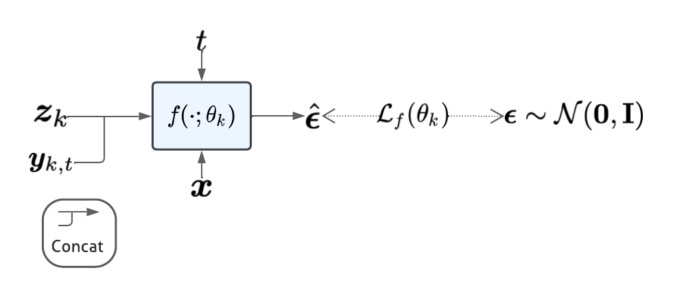
Figure 5: The denoising network $f(\cdot;\theta_{k})$ that estimates the noise $\bm{\epsilon}$ at time-step $t$. It takes the intermediate latent variable of the diffusion process $\bm{y}_{k,t}$, the latent code from the shallow mapping stage $\bm{z}_{k}$, the query image $\bm{x}$, and the current time-step $t$ as input. Note that $\bm{y}_{k,t}$ and $\bm{z}_{k}$ are concated together. $\mathcal{L}_{f}$ measures the L2 norm between the estimation and the sampled noise $\bm{\epsilon}$.

IV Experiments and Results

We evaluate our method on two medical imaging benchmarks: Tuberculosis chest X-ray dataset [15] and the ISIC Melanoma skin cancer dataset [16]. The Tuberculosis chest X-ray dataset consists of X-ray images of 3500 patients with Tuberculosis and 3500 patients without Tuberculosis. The ISIC Melanoma skin cancer dataset contains images of 5105 patients with malignant skin cancer and 5500 patients with benign skin cancer. We choose a range of baseline methods that cover various architectures: CNNs, transformers, and hybrid models with both CNNs and transformers. Note that we only train models on the original domain, in other words, where no data augmentation is applied to the training set image.

We compare our method with baselines that are widely used in medical image analysis with classification accuracy and confidence calibration error as metrics [6, 7, 2, 3, 36, 37, 38, 39, 8], such as the ResNet [40] family, Vision Transformers (ViTs) [30]. In addition, we evaluate other methods that are widely used in natural image classification but have not been investigated in previous works on robust medical image classification tasks (see methods column in Table. I for the complete list). We hope that this work can inspire future works that dive deeper into this topic.

For the chest X-ray dataset, the sample quantity for training/validation/testing set split is $5670/630/700$, and all samples are binary labeled. For the ISIC skin cancer dataset, the sample quantity for training/validation/testing set split is $7605/1000/2000$, and all samples are binary labeled. We choose $K=5$, $M=20$, $T=1000$, and $\alpha_{1}=1-10^{-4}$, $\alpha_{T}=0.98$ as hyper-parameter configuration for our method.

IV-A Robustness evaluation

We simulate input image variation caused by differences in acquisition machines at test time by manipulating a range of image properties: (i) adding Gaussian noise, (ii) reducing resolution, and (iii) decreasing contrast. In addition, we evaluate our method against adversarial samples that are generated by three attack strategies: (i) Fast Gradient Sign Method (FGSM) [41], (ii) Projected Gradient Descent (PGD) [42], and (iii) Auto-PGD [43].

For reference, we provide the results of experiments conducted in the original domain; in other words, where no transformations are applied to the input image. In Table. I, we separate baseline methods into four groups based on their different fundamental architectures: convolutional neural networks (CNNs), transformers, CNN and transformer hybrid models, and self-ensemble models. As shown in Table. I, the classification accuracy of all methods is very close to each other on the chest X-ray dataset and near perfect (all beyond $99.00\%$). On the other hand, ResNet-18 reaches the top accuracy on the ISIC dataset. One possible reason is its comparatively limited parameter quantity, which helps reduce the chance of overfitting the training data.

TABLE I: Comparison with state-of-the-art methods on two benchmark datasets in their original domain. We report the mean and the standard deviation of the classification accuracy (%) $\uparrow$, averaged over three runs.

Methods	Chest X-ray	ISIC
ResNet-18 [40]	$99.86\pm 0.00$	$\textbf{95.02}\pm\textbf{0.15}$
ResNet-50 [40]	$\textbf{99.93}\pm\textbf{0.07}$	$94.69\pm 0.19$
EfficientNetV2-L [44]	$99.33\pm 0.18$	$91.26\pm 0.23$
DeiT-B [45]	$99.91\pm 0.07$	$94.34\pm 0.25$
ViT-B [30]	$99.75\pm 0.24$	$92.93\pm 0.29$
Swin-B [46]	$99.86\pm 0.20$	$94.57\pm 0.17$
ConViT-B [47]	$99.76\pm 0.14$	$94.41\pm 0.13$
MedViT-B [18]	$99.86\pm 0.12$	$92.42\pm 0.06$
SEViT [19]	$99.91\pm 0.07$	$93.56\pm 0.16$
Our method	$99.90\pm 0.14$	$94.18\pm 0.24$

TABLE II: Comparison with state-of-the-art methods on two benchmark datasets where we simulated the image variations raised from different acquisition conditions. We report the mean and the standard deviation of the classification accuracy (%) $\uparrow$, averaged over three runs.

Methods	Chest X-ray				ISIC
	Gaussian noise		Low resolution	Contrast	Gaussian noise		Low resolution	Contrast
	$\mathbb{g}=0.50$	$\mathbb{g}=1.00$	$w=4.00$	$r=0.70$	$\mathbb{g}=0.50$	$\mathbb{g}=1.00$	$w=4.00$	$r=0.70$
ResNet-18	$50.00\pm 0.00$	$50.00\pm 0.00$	$50.00\pm 0.00$	$99.57\pm 0.11$	$50.56\pm 2.23$	$49.64\pm 0.94$	$81.48\pm 2.88$	$92.37\pm 0.28$
ResNet-50	$50.00\pm 0.00$	$50.38\pm 0.54$	$50.00\pm 0.00$	$\textbf{99.86}\pm\textbf{0.20}$	$51.02\pm 0.00$	$54.34\pm 4.69$	$80.48\pm 3.40$	$92.42\pm 0.09$
EfficientNetV2-L	$50.00\pm 0.00$	$50.00\pm 0.00$	$96.86\pm 0.42$	$93.10\pm 0.70$	$48.98\pm 0.00$	$48.98\pm 0.00$	$89.73\pm 0.31$	$88.45\pm 1.50$
DeiT-B	$68.86\pm 5.36$	$57.57\pm 6.25$	$94.43\pm 2.89$	$99.57\pm 0.00$	$69.32\pm 2.04$	$64.69\pm 1.92$	$87.75\pm 0.15$	$92.54\pm 0.67$
ViT-B	$74.34\pm 2.89$	$57.76\pm 4.18$	$94.71\pm 0.71$	$97.14\pm 0.12$	$71.90\pm 8.86$	$55.42\pm 4.00$	$89.72\pm 0.37$	$91.58\pm 0.40$
Swin-B	$59.81\pm 0.04$	$50.00\pm 0.00$	$59.29\pm 3.25$	$98.29\pm 2.42$	$67.43\pm 1.72$	$63.93\pm 0.83$	$88.44\pm 0.60$	$91.34\pm 0.25$
ConViT-B	$76.57\pm 4.69$	$55.00\pm 2.53$	$94.62\pm 1.67$	$99.33\pm 0.29$	$70.86\pm 1.69$	$60.83\pm 4.08$	$90.62\pm 0.90$	$92.93\pm 0.04$
MedViT-B	$73.00\pm 3.05$	$52.95\pm 2.20$	$96.24\pm 0.57$	$94.67\pm 0.49$	$61.63\pm 2.02$	$47.58\pm 2.15$	$\textbf{91.46}\pm\textbf{0.46}$	$90.92\pm 0.37$
SEViT	$69.19\pm 3.27$	$62.24\pm 4.36$	$97.76\pm 0.33$	$97.15\pm 0.20$	$67.04\pm 2.59$	$54.42\pm 3.64$	$90.16\pm 0.72$	$92.00\pm 0.14$
Our method	$\textbf{78.33}\pm\textbf{0.69}$	$\textbf{66.33}\pm\textbf{2.07}$	$\textbf{98.90}\pm\textbf{0.49}$	$97.86\pm 0.23$	$\textbf{73.16}\pm\textbf{2.66}$	$\textbf{69.93}\pm\textbf{2.35}$	$91.17\pm 0.36$	$\textbf{93.14}\pm\textbf{0.24}$

To evaluate the robustness of our model against Gaussian noise, we first define our transformation as $\mathcal{T}_{gn}(\bm{x})=\bm{x}+\mathbb{g}\epsilon$, where $\epsilon\sim\mathcal{N}(\mathbf{0},\mathbf{I})$, and $\mathbb{g}$ controls the scale of the noise that is added to the image $\bm{x}$. As $\mathbb{g}$ becomes larger, the transformed image $\bm{x}^{\prime}$ tends to be more different than its original copy $\bm{x}$. Hence, it is very challenging for a classifier that is only trained on the ideal domain of $\bm{x}$ (without adding noise) to predict the corresponding ground-truth $\bm{y}$ correctly. As illustrated in Table. II, we conduct experiments on two benchmarks with $\mathbb{g}=0.50$. Our method surpasses all baseline methods in classification accuracy by a large margin. Our experimental results also reveal that methods based purely on convolutional neural networks (CNNs), particularly the ResNet family, fail to generalize well on Gaussian noise perturbation.

In addition, we evaluate the performance of our method under the condition where the testing data is of low resolution. To this end, we transform the images in the testing set to low-resolution images by downsampling by a factor $w$. Hence, the resolution of the transformed image $\bm{x}^{\prime}$ is $(\lfloor H/w\rfloor,\lfloor W/w\rfloor)$, where $(H,W)$ is the resolution of the original image $\bm{x}$, and $\lfloor\cdot\rfloor$ is the floor function. In this way, transformed images lose a degree of detail compared to their original copy $\bm{x}$, which may impact the performance of a classifier. In Table. II, our method outperforms other baselines regarding classification accuracy in most cases except $w=4.00$ on the ISIC dataset. However, its performance is still comparable with the winner MedViT, with only $0.29\%$ accuracy drop.

Furthermore, we investigate another factor that may impact the performance: image contrast. We transform the image with $\mathcal{T}_{ctr}(\bm{x})=r(\bm{x}-\mu_{x})+\mu_{x}$, here $\mu_{x}$ is the mean value of all pixels in the image $\bm{x}$ across all channels, and $r$ controls the contrast level. In our experiments, we choose the contrast level $r=0.70$ for evaluation. As illustrated in Table. II, our method surpasses all baselines on the ISIC dataset. In addition, we observe that lower-contrast images lead to a more significant performance degradation than higher-contrast copies.

To complement previous studies on adversarial attack robustness and defense mechanisms in medical image analysis and classification [48, 49, 19, 50, 20], we test our method together with baselines. Here, we follow the setting introduced in [19] that applies adversarial perturbation $\mathcal{T}_{\mathrm{adv}}(\cdot)$ on image $\bm{x}$ based on the gradient of the backbone image recognition model $\mathcal{M}(\cdot)$, such that $\|\bm{x}-\mathcal{T}_{\mathrm{adv}}(\bm{x})\|_{\infty}\leq\varepsilon$ and $\mathcal{M}(\bm{x})\neq\mathcal{M}(\mathcal{T}_{\mathrm{adv}}(\bm{x}))$. In Table. III, our method shows superior performance under adversarial attacks with $\varepsilon=0.03$. This huge performance boost compared to baselines reflects the importance of utilizing consistent feature representations in the design of the shallow mapping stage, where perturbations such as adversarial noise can only bring limited impact on the inner structure of the extracted image features.

TABLE III: Comparison with state-of-the-art methods on two benchmarks with 3 types of adversarial attacks: FGSM, PGD, and AutoPGD. We report the mean and the standard deviation of the classification accuracy (%) $\uparrow$, averaged over three runs.

Methods	Chest X-ray			ISIC
	FGSM	PGD	AutoPGD	FGSM	PGD	AutoPGD
	$\varepsilon=0.03$
ResNet-18	$47.50\pm 2.24$	$0.00\pm 0.00$	$0.00\pm 0.00$	$50.56\pm 1.87$	$0.00\pm 0.00$	$0.00\pm 0.00$
ResNet-50	$46.72\pm 3.40$	$0.00\pm 0.00$	$0.00\pm 0.00$	$55.32\pm 0.24$	$0.00\pm 0.00$	$0.00\pm 0.00$
EfficientNetV2-L	$34.28\pm 1.02$	$0.19\pm 0.07$	$0.14\pm 0.12$	$19.75\pm 6.24$	$0.00\pm 0.00$	$0.00\pm 0.00$
DeiT-B	$35.28\pm 1.76$	$0.00\pm 0.00$	$0.00\pm 0.00$	$26.33\pm 7.15$	$0.00\pm 0.00$	$0.00\pm 0.00$
ViT-B	$15.38\pm 3.68$	$0.14\pm 0.12$	$0.00\pm 0.00$	$22.20\pm 8.22$	$0.29\pm 0.17$	$0.00\pm 0.00$
Swin-B	$71.95\pm 3.03$	$0.00\pm 0.00$	$0.00\pm 0.00$	$24.49\pm 1.08$	$0.00\pm 0.00$	$0.00\pm 0.00$
ConViT-B	$20.52\pm 2.66$	$0.00\pm 0.00$	$0.00\pm 0.00$	$35.95\pm 0.74$	$0.02\pm 0.02$	$0.00\pm 0.00$
MedViT-B	$10.29\pm 4.50$	$2.95\pm 2.10$	$0.38\pm 0.36$	$23.93\pm 6.28$	$0.00\pm 0.00$	$0.00\pm 0.00$
SEViT	$85.90\pm 3.39$	$92.76\pm 0.86$	$94.24\pm 1.36$	$54.15\pm 3.56$	$51.52\pm 4.99$	$57.30\pm 8.74$
Our method	$\textbf{94.86}\pm\textbf{0.20}$	$\textbf{96.10}\pm\textbf{0.94}$	$\textbf{96.05}\pm\textbf{1.48}$	$\textbf{60.15}\pm\textbf{4.93}$	$\textbf{61.60}\pm\textbf{4.53}$	$\textbf{61.30}\pm\textbf{2.70}$

IV-B Confidence calibration

In addition to evaluating classification accuracy, we also consider if the prediction (classification) probability $\mathrm{Pr}(\bm{y}=c\mid\bm{x})$ is well-calibrated. A well-calibrated prediction probability, in other words, a well-calibrated model $\mathcal{M}(\cdot)$, typically refers to: for all predictions with confidence of $p=\mathrm{Pr}(\mathcal{M}(\bm{x})=c)$, the fraction of those predictions that are correct is approximately $p$ [51]. Our method calculates the probability of predicting a specific class $c$ by model averaging as indicated in Eq. 25. Here, we set $\iota=0.1737$ for the chest X-ray dataset and $\iota=0.3162$ for the ISIC dataset. Note that $\iota$ is a tunable hyperparameter. Its value depends on the nature of the data and the training setup. In this work, $\iota$ is tuned for the best calibration performance possible.

When the quality of the testing set is far from perfect, it becomes more crucial to obtain a well-calibrated predicted probability because it helps clinicians avoid making wrong decisions when the model can express potentially incorrect results in a way that provides low predicted probability. To better illustrate the performance of our method and baselines on confidence calibration under the above condition, we focus on experimental settings where the classification accuracy is comparatively lower (Sec. IV-A). Across all experimental settings, we observe that the performance of all methods suffer when Gaussian noise is added to the input image. Hence, we measure the Expected Calibration Error (ECE) [51] with ten bins (calculated in Eq. 32, where $B_{i}$ denotes the set of indices of samples that fall into bin $i$, $u$ is the number of samples, $\mathbf{acc}(B_{i})$ is the empirical accuracy for bin $i$, i.e., the fraction of correct predictions in the bin, and $\mathbf{conf}(B_{i})$ is the average predicted probability for bin $i$) and shows the performance of all methods (Fig. 6) after adding Gaussian noise. For completeness, we also provide results tested in the original domain.

$$\mathrm{ECE}_{10}:=\sum_{i=1}^{10}\frac{|B_{i}|}{u}\Big{|}\mathbf{acc}(B_{i})-\mathbf{conf}(B_{i})\Big{|}.$$ (32)

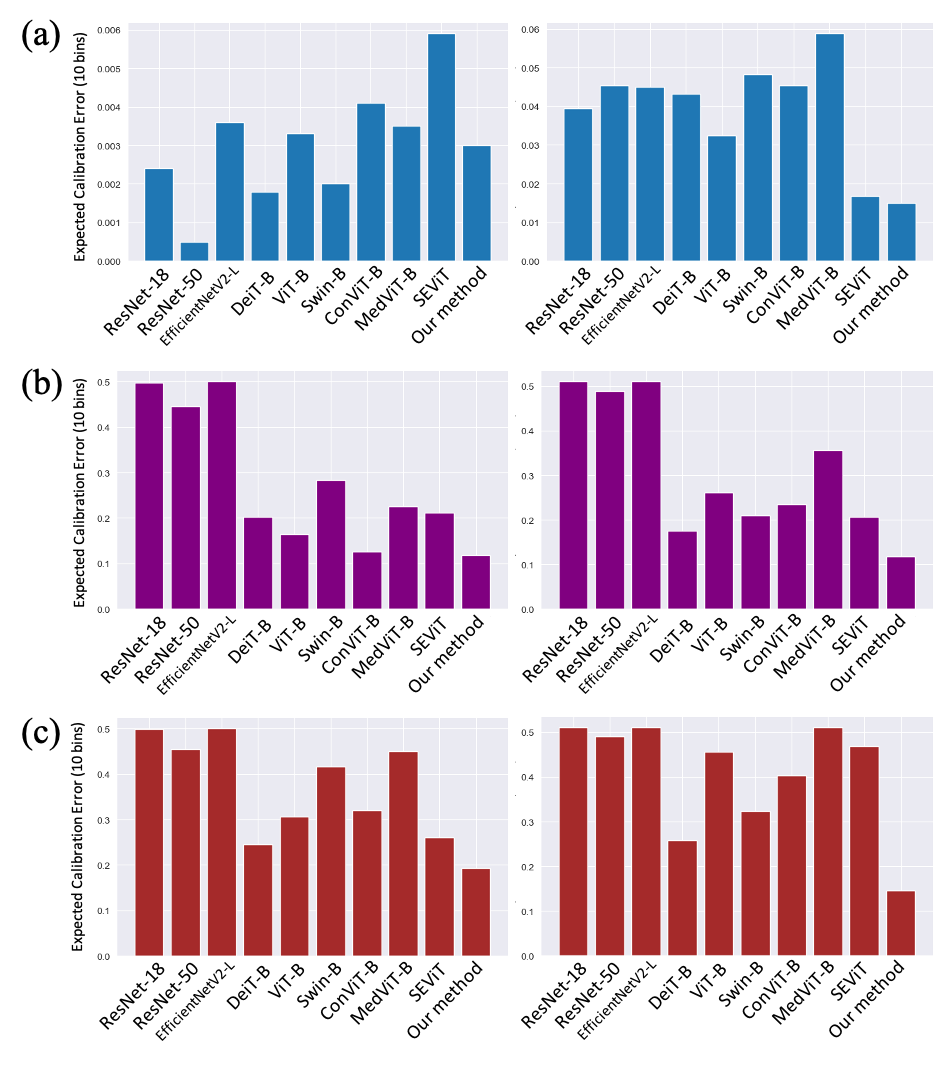
Figure 6: Plot of Expected Calibration Error (ECE) with ten bins on two benchmarks datasets (the chest X-ray dataset and the ISIC dataset are on the left and the right hand-side, respectively): (a) the ECE when tested on the original domain, (b) the ECE when $\mathbb{g}=0.50$ Gaussian noise is added, and (c) the ECE when $\mathbb{g}=1.00$ Gaussian noise is added.

As illustrated in Fig. 6, the proposed method outperforms all baselines in all experiment settings (except for the test on the original domain on the chest X-ray dataset) for achieving the lowest ECE. In the test on the original domain on the chest X-ray dataset, Fig. 6 shows nearly perfect ECE (all below $0.006$) and minimal ECE difference between methods.

IV-C Quantifying prediction uncertainty

As discussed in Sec. IV-B, a well-calibrated model can express its prediction uncertainty by evaluating the predicted probability. Higher probability reflects that the model is more confident in its prediction and less uncertain. However, a poorly calibrated model is usually over-confident in its incorrect predictions [51] and hence fails to adequately express its intrinsic uncertainty in terms of predicted probability.

To properly access the model’s uncertainty, we introduce another strategy for quantifying prediction uncertainty without the prior assumption of perfect confidence calibration. Inspired by works done by Gal et al. and Han et al. [52, 28], together with the nature of our Nested-ensemble, we propose to use the Prediction Interval Width (PIW) and the Prediction Variance (PV) as means of quantifying uncertainty. For a set of predictions $S_{\mathrm{ne}}$ which is formed by uniting $K$ candidate groups (each contains $M$ predictions) in our formulation Sec. III-C such that $|S_{\mathrm{ne}}|=KM$, PIW and PV for predicting a specific class $c$ are calculated as follows, here $\hat{\bm{y}}_{i}\in S_{\mathrm{ne}}$, $\mathcal{Q}_{n}(\cdot)$ calculates the $n^{\mathrm{th}}$ percentile, and $(\cdot)^{\bigodot 2}$ denotes the element-wise square:

$$\mathrm{PIW}_{c}:=\Big{[}\mathcal{Q}_{97.5}(S_{\mathrm{ne}})-\mathcal{Q}_{2.5}(S_{\mathrm{ne}})\Big{]}_{c},$$ (33)

$$\mathrm{PV}_{c}:=\frac{1}{KM}\sum_{i=1}^{KM}\Big{[}(\hat{\bm{y}}_{i}-\bar{\bm{y}})^{\bigodot 2}\Big{]}_{c},\quad\bar{\bm{y}}=\frac{\sum_{i=1}^{KM}\hat{\bm{y}}_{i}}{KM}.$$ (34)

Similar to the previous section, we aim to illustrate how our method’s uncertainty behaves when the prediction accuracy is far from perfect. This experiment shows this uncertainty measurement under Gaussian noise simulation transformation ($\mathbb{g}=1.00$) on the chest X-ray dataset. The results, as presented in Table. IV, reveal distinct uncertainty patterns for different classes. For class 1 (normal) predictions, the PIW and PV metrics indicate high uncertainty; both metrics exhibit large values regardless of whether the prediction is potentially correct or incorrect. In contrast, for class 2 (tuberculosis patient) predictions, the PIW and PV values associated with correct predictions are markedly higher than those for incorrect predictions. This suggests that our model demonstrates a higher degree of certainty when predicting class 2 compared to class 1.

TABLE IV: PIWs and PVs for experiment on Gaussian noise transformation with $\mathbb{g}=1.00$ on the chest X-ray dataset.

		PIW	PV
Class 1 (Normal)	Correct	$0.9998$	$0.2278$
	Incorrect	$0.9997$	$0.2235$
Class 2 (Tuberculosis)	Correct	$0.4330$	$0.0630$
	Incorrect	$0.8600$	$0.1799$

V Conclusion

In this work, we addressed the crucial challenge of robustness in medical image classification. We proposed a novel architecture inspired by the success of transformers, further enhanced by an innovative three-stage approach consisting of Shallow Mapping for consistent representation learning, Corrective Diffusion for refining draft predictions, and a new ensemble technique named Nested-Ensemble. The proposed framework not only maintains high accuracy amidst complex image distortions but also showcases superior performance over existing state-of-the-art methods. In addition, we provide an analysis of model confidence and prediction uncertainty, further providing a mechanism for improving the trustworthiness of the model in real clinical contexts.

Appendix

I Derivations

I-A Derivation for the forward sampling distribution in the corrective diffusion stage

We provide the derivation for the forward sampling distribution $q(\bm{y}_{k,t}\mid\bm{y}_{k,0},\bm{z}_{k},\bm{x})$ for an arbitrary time-step $t$ of the $k^{\mathrm{th}}$ base learner as follows:

From Eq. 11, we have

$$\bm{y}_{k,t} =\sqrt{\alpha_{t}}\bm{y}_{k,t-1}+(1-\sqrt{\alpha_{t}})(\bm{z}_{k}+e(\bm{x}))+\sqrt{1-\alpha_{t}}\bm{\epsilon}^{*}_{t-1}$$

$$=\sqrt{\alpha_{t}}(\sqrt{\alpha_{t-1}}\bm{y}_{k,t-2}+(1-\sqrt{\alpha_{t-1}})(\bm{z}_{k}+e(\bm{x}))$$

$$\quad+\sqrt{1-\alpha_{t-1}}\bm{\epsilon}^{*}_{t-2})+(1-\sqrt{\alpha_{t}})(\bm{z}_{k}+e(\bm{x}))$$

$$\quad+\sqrt{1-\alpha_{t}}\bm{\epsilon}^{*}_{t-1}$$

$$=\sqrt{\alpha_{t}\alpha_{t-1}}\bm{y}_{k,t-2}+(\sqrt{\alpha_{t}}-\sqrt{\alpha_{t}\alpha_{t-1}})(\bm{z}_{k}+e(\bm{x}))$$

$$\quad+\sqrt{\alpha_{t}-\alpha_{t}\alpha_{t-1}}\bm{\epsilon}^{*}_{t-2}+(1-\sqrt{\alpha_{t}})(\bm{z}_{k}+e(\bm{x}))$$

$$\quad+\sqrt{1-\alpha_{t}}\bm{\epsilon}^{*}_{t-1}$$

$$=\sqrt{\alpha_{t}\alpha_{t-1}}\bm{y}_{k,t-2}+(1-\sqrt{\alpha_{t}\alpha_{t-1}})(\bm{z}_{k}+e(\bm{x}))$$

$$\quad+\sqrt{\alpha_{t}-\alpha_{t}\alpha_{t-1}+1-\alpha_{t}}\bm{\epsilon}_{t-2}$$

$$=\dotsc\mathrm{(recursion)}$$

$$=\sqrt{\prod_{i=1}^{t}\alpha_{i}}\bm{y}_{k,0}+\left(1-\sqrt{\prod_{i=1}^{t}\alpha_{i}}\right)(\bm{z}_{k}+e(\bm{x}))$$

$$\quad+\sqrt{1-\prod_{i=1}^{t}\alpha_{i}}\bm{\epsilon}_{0}$$

$$=\sqrt{\bar{\alpha}_{t}}\bm{y}_{k,0}+(1-\sqrt{\bar{\alpha}_{t}})(\bm{z}_{k}+e(\bm{x}))+\sqrt{1-\bar{\alpha}_{t}}\bm{\epsilon}_{0},$$

where $\{\bm{\epsilon}^{*}_{t-1},\bm{\epsilon}^{*}_{t-2},\bm{\epsilon}_{t-2},\bm{\epsilon}_{0}\}\stackrel{{\scriptstyle\text{iid}}}{{\sim}}\mathcal{N}(\mathbf{0},\mathbf{I})$. This yields to a Gaussian reparameterization in the form of the following:

$$\mathcal{N}(\bm{y}_{k,t};\sqrt{\bar{\alpha}_{t}}\bm{y}_{k,0}+\left(1-\sqrt{\bar{\alpha}_{t}}\right)(\bm{z}_{k}+e(\bm{x})),(1-\bar{\alpha}_{t})\mathbf{I}).$$

In the above recursive derivation, one thing to note is that we interpret the terms $\sqrt{\alpha_{t}-\alpha_{t}\alpha_{t-1}}\bm{\epsilon}^{*}_{t-2}$ and $\sqrt{1-\alpha_{t}}\bm{\epsilon}^{*}_{t-1}$ as two independent Gaussian random variables that follows $\mathcal{N}(\mathbf{0},(\alpha_{t}-\alpha_{t}\alpha_{t-1})\mathbf{I})$ and $\mathcal{N}(\mathbf{0},(1-\alpha_{t})\mathbf{I})$, respectively. Note that the sum of two independent Gaussian random variables holds as a Gaussian random variable, with the mean of the sum of two means and variance being the sum of two variances. This enables us to consider the result of $\sqrt{\alpha_{t}-\alpha_{t}\alpha_{t-1}}\bm{\epsilon}^{*}_{t-2}+\sqrt{1-\alpha_{t}}\bm{\epsilon}^{*}_{t-1}$ as a new random variable that is sampled from $\mathcal{N}(\mathbf{0},(1-\alpha_{t}\alpha_{t-1})\mathbf{I})$.

I-B Derivation for the forward transition posterior in the corrective diffusion stage

We provide the derivation for the parametric form of the forward transition posterior $q(\bm{y}_{k,t-1}\mid\bm{y}_{k,t},\bm{y}_{k,0},\bm{z}_{k},\bm{x})$ in the corrective diffusion stage for the $k^{\mathrm{th}}$ base learner as follows:

$$q(\bm{y}_{k,t-1}\mid\bm{y}_{k,t},\bm{y}_{k,0},\bm{z}_{k},\bm{x})$$

$$= \>\frac{q(\bm{y}_{k,t}\mid\bm{y}_{k,t-1},\bm{y}_{k,0},\bm{z}_{k},\bm{x})q(\bm{y}_{k,t-1}\mid\bm{y}_{k,0},\bm{z}_{k},\bm{x})}{q(\bm{y}_{k,t}\mid\bm{y}_{k,0},\bm{z}_{k},\bm{x})}$$

$$= \>\frac{\mathcal{N}(\bm{y}_{k,t};\sqrt{\alpha_{t}}\bm{y}_{k,t-1}+(1-\sqrt{\alpha_{t}})(\bm{z}_{k}+e(\bm{x})),(1-\alpha_{t})\mathbf{I})}{\mathcal{N}(\bm{y}_{k,t};\sqrt{\bar{\alpha}_{t}}\bm{y}_{k,0}+\left(1-\sqrt{\bar{\alpha}_{t}}\right)(\bm{z}_{k}+e(\bm{x})),(1-\bar{\alpha}_{t})\mathbf{I})}$$

$$\>\mathcal{N}(\bm{y}_{k,t-1};\sqrt{\bar{\alpha}_{t-1}}\bm{y}_{k,0}+\left(1-\sqrt{\bar{\alpha}_{t-1}}\right)(\bm{z}_{k}+e(\bm{x})),$$

$$\>(1-\bar{\alpha}_{t-1})\mathbf{I})$$

$$\propto \>\exp\Bigg{\{}-\Bigg{[}\frac{(\bm{y}_{k,t}-\sqrt{\alpha_{t}}\bm{y}_{k,t-1}-(1-\sqrt{\alpha_{t}})(\bm{z}_{k}+e(\bm{x})))^{2}}{2(1-\alpha_{t})}$$

$$\>+\frac{(\bm{y}_{k,t-1}-\sqrt{\bar{\alpha}_{t-1}}\bm{y}_{k,0}-(1-\sqrt{\bar{\alpha}_{t-1}})(\bm{z}_{k}+e(\bm{x})))^{2}}{2(1-\bar{\alpha}_{t-1})}$$

$$\>-\frac{(\bm{y}_{k,t}-\sqrt{\bar{\alpha}_{t}}\bm{y}_{k,0}-(1-\sqrt{\bar{\alpha}_{t}})(\bm{z}_{k}+e(\bm{x})))^{2}}{2(1-\bar{\alpha}_{t})}\Bigg{]}\Bigg{\}}$$

$$= \>\exp\Bigg{\{}-\frac{1}{2}\Bigg{[}\frac{\alpha_{t}\bm{y}_{t-1}^{2}}{1-\alpha_{t}}$$

$$\>+\frac{((2\sqrt{\alpha_{t}}-2\alpha_{t})(\bm{z}_{k}+e(\bm{x}))-2\sqrt{\alpha_{t}}\bm{y}_{k,t})\bm{y}_{k,t-1}}{1-\alpha_{t}}$$

$$\>+\frac{\bm{y}_{k,t-1}^{2}-2\sqrt{\bar{\alpha}_{t-1}}\bm{y}_{k,t-1}\bm{y}_{k,0}}{1-\bar{\alpha}_{t-1}}$$

$$\>-\frac{2(1-\sqrt{\bar{\alpha}_{t-1}})(\bm{z}_{k}+e(\bm{x}))\bm{y}_{k,t-1}}{1-\bar{\alpha}_{t-1}}$$

$$\>+C(\bm{y}_{k,t},\bm{y}_{k,0},\bm{z}_{k},\bm{x})\Bigg{]}\Bigg{\}}$$

$$\propto \>\exp\Bigg{\{}-\frac{1}{2}\Bigg{[}\Bigg{(}\frac{\alpha_{t}}{1-\alpha_{t}}+\frac{1}{1-\bar{\alpha}_{t-1}}\Bigg{)}\bm{y}_{k,t-1}^{2}$$

$$\>+\Bigg{(}\frac{(2\sqrt{\alpha_{t}}-2\alpha_{t})(\bm{z}_{k}+e(\bm{x}))-2\sqrt{\alpha_{t}}\bm{y}_{k,t}}{1-\alpha_{t}}$$

$$\>+\frac{-2\sqrt{\bar{\alpha}_{t-1}}\bm{y}_{k,0}-2(1-\sqrt{\bar{\alpha}_{t-1}})(\bm{z}_{k}+e(\bm{x}))}{1-\bar{\alpha}_{t-1}}\Bigg{)}$$

$$\>\bm{y}_{k,t-1}\Bigg{]}\Bigg{\}}$$

$$\propto \>\exp\Bigg{\{}-\frac{1}{2}\Bigg{(}\frac{1-\bar{\alpha}_{t}}{(1-\alpha_{t})(1-\bar{\alpha}_{t-1})}\Bigg{)}\Bigg{(}\bm{y}_{k,t-1}^{2}$$

$$\>-2\tilde{\bm{\mu}}_{q}(\bm{y}_{k,t},\bm{y}_{k,0},\bm{z}_{k},\bm{x})\bm{y}_{k,t-1}$$

$$\>+C(\bm{y}_{k,t},\bm{y}_{k,0},\bm{z}_{k},\bm{x})\Bigg{)}\Bigg{\}}$$

$$\propto \>\mathcal{N}\Bigg{(}\bm{y}_{k,t-1};\tilde{\bm{\mu}}_{q}(\bm{y}_{k,t},\bm{y}_{k,0},\bm{z}_{k},\bm{x}),\bm{\Sigma}_{q}(t)\Bigg{)},$$

where

$$\tilde{\bm{\mu}}_{q}(\bm{y}_{k,t},\bm{y}_{k,0},\bm{z}_{k},\bm{x})$$

$$:=\; \frac{\sqrt{\alpha_{t}}(1-\bar{\alpha}_{t-1})}{1-\bar{\alpha}_{t}}\bm{y}_{k,t}+\frac{\sqrt{\bar{\alpha}_{t-1}}(1-\alpha_{t})}{1-\bar{\alpha}_{t}}\bm{y}_{k,0}$$

$$-\left(\frac{\sqrt{\alpha_{t}}(1-\bar{\alpha}_{t-1})+\sqrt{\bar{\alpha}_{t-1}}(1-\alpha_{t})}{1-\bar{\alpha}_{t}}-1\right)$$

$$\cdot(\bm{z}_{k}+e(\bm{x})),$$

and

$$\bm{\Sigma}_{q}(t):=\left(\frac{(1-\alpha_{t})(1-\bar{\alpha}_{t-1})}{1-\bar{\alpha}_{t}}\right)\mathbf{I}.$$

In the above derivation, $C(\bm{y}_{k,t},\bm{y}_{k,0},\bm{z}_{k},\bm{x})$ denotes a constant term with respect to $\bm{y}_{k,t-1}$ computed with $\bm{y}_{k,t}$, $\bm{y}_{k,0}$, $\bm{z}_{k}$, and $\bm{x}$. Note that we reintroduce this constant term at the penultimate step to complete the square.

II Implementation Details

For completeness, we provide the implementation details for our networks including the backbone image recogbnition model, the shallow mapping function, and the denoising network.

II-A Backbone image recognition model

We chose ViT-B/16 as our backbone model to extract image features. The input 3-channel image of resolution $224\times 224$ is divided into a fixed number of patches, each of size $16\times 16$. These patches are linearly embedded to dimension 768, resulting in a sequence of 196 flattened patch embeddings. A [CLS] token is edded to the sequence, and sinusoidal position embedding is added to each patch token to encode relative positional information. This architecture has 12 transformer encoder blocks, each consisting of multi-head self-attention with 12 attention heads, plus a feed-forward network with 3072 neurons. The classification head is implemented with a linear projection matrix of size $2\times 768$, and it is applied to the [CLS] token for obtaining the classification result.

II-B Shallow mapping function

The shallow mapping component $g(\cdot;\psi_{k})$ is implemented with a feed-forward neural network consisting of an input layer of size $768\times 196$, three fully connected hidden layers with size $\{4096,2048,128\}$, and an output layer of size 2. ReLU activation function is used between layers.

II-C Denoising network

The additional image encoder $e(\cdot)$ is implemented with a feed-forward neural network consisting of an input layer of size $224\times 224\times 3$, two fully connected hidden layers with size $\{300,100\}$, and an output layer of size 4096. 1D batch normalization and ReLU activation are used between layers. The time embedding is implemented with a learnable embedding dictionary with discrete time-step $t$ as the key and an output vector of size 4096 as the corresponding value. The function $f(\bm{y}_{k,t},\bm{z}_{k},\bm{x},t;\theta_{k})$ first concatenates $\bm{y}_{k,t}$ and $\bm{z}_{k}$, then maps the resulting vector to a new vector of size 4096 through a linear transformation. This new vector is multiplied with the time embedding and then with the encoded $e(\bm{x})$. After that, the resulting vector is applied with 1D batch normalization and Softplus function. At last, a linear layer of size equaling the size of $\bm{y}_{k,t}$ is introduced to produce the output.

III Training

We provide the training pseudo-code for our method in Algorithm 2.

Algorithm 2 Training

0:  Training data $\mathcal{D}=\{(\bm{x}_{i},\bm{y}_{i})\}_{i=1}^{O}$

0:  Backbone model parameters $\gamma,\Phi,\omega$

1:  Initialize $\gamma,\Phi,\omega$

2:  repeat

3:     for each $(\bm{x}_{i},\bm{y}_{i})$ in $\mathcal{D}$ do

4:        $\bm{\hat{}}{\bm{y}}_{b}=h((l_{L}\circ l_{L-1}\circ\dotsc\circ l_{1}\circ l_{emb})(\bm{x}_{i};\omega,\Phi,\gamma)_{0})$

5:        Compute $\mathcal{L}_{\mathrm{init}}$ using $\bm{\hat{}}{\bm{y}}_{b}$ and $\bm{y}_{i}$ (in Eq. 26)

6:        Take numerical optimization step on $\nabla_{\gamma,\Phi,\omega}\mathcal{L}_{\mathrm{init}}$

7:     end for

8:  until Converge

9:  return  $\gamma,\Phi,\omega$

9:  Backbone model parameters $\gamma,\Phi,\omega$

9:  Shallow mapping parameters for $K$ base learners $\psi_{1},\dotsc,\psi_{K}$

10:  for $k$ in $\{1,\dotsc,K\}$ do

11:     Initialize $\psi_{k}$

12:     repeat

13:        for each $(\bm{x}_{i},\bm{y}_{i})$ in $\mathcal{D}$ do

14:           $\bm{z}_{k}=s(\bm{x}_{i};\psi_{k},\phi_{1:k},\gamma)$

15:           Compute $\mathcal{L}_{g}$ using $\bm{z}_{k}$ and $\bm{y}_{i}$ (in Eq. 27)

16:           Take numerical optimization step on $\nabla_{\psi_{k}}\mathcal{L}_{g}$

17:        end for

18:     until Converge

19:  end for

20:  return  $\psi_{1},\dotsc,\psi_{K}$

20:  Parameters $\gamma,\Phi,\omega,\psi_{1},\dotsc,\psi_{K}$

20:  Denoising network parameters for $K$ base learners $\theta_{1},\dotsc,\theta_{K}$

21:  for $k$ in $\{1,\dotsc,K\}$ do

22:     Initialize $\theta_{k}$

23:     repeat

24:        for each $(\bm{x}_{i},\bm{y}_{i})$ in $\mathcal{D}$ do

25:           $\bm{z}_{k}=s(\bm{x}_{i};\psi_{k},\phi_{1:k},\gamma)$

26:           Draw $t\sim\mathrm{Uniform}(\{1,\dotsc,T\})$

27:           Draw $\bm{\epsilon}\sim\mathcal{N}(\mathbf{0},\mathbf{I})$

28:           Compute $\mathcal{L}_{f}$ using $\bm{\epsilon},\bm{z}_{k},\bm{y}_{i},\bm{x}_{i},t$ (in Eq. 29)

29:           Take numerical optimization step on $\nabla_{\theta_{k}}\mathcal{L}_{f}$

30:        end for

31:     until Converge

32:  end for

33:  return  $\theta_{1},\dotsc,\theta_{K}$

IV Additional Experiments Results

IV-A Robustness evaluation under resolution difference

We provide complete evaluation when $w=0.00,4.00,8.00$ on chest X-ray dataset and ISIC dataset in Table. V.

TABLE V: Comparison with state-of-the-art methods on two benchmark datasets where we vary the image resolution. We report the mean and the standard deviation of the classification accuracy (%) $\uparrow$, averaged over three runs.

Methods	Chest X-ray			ISIC
	Low resolution
	$w=0.00$ (ref)	$w=4.00$	$w=8.00$	$w=0.00$ (ref)	$w=4.00$	$w=8.00$
ResNet-18	$99.86\pm 0.00$	$50.00\pm 0.00$	$50.00\pm 0.00$	$95.02\pm 0.15$	$81.48\pm 2.88$	$67.59\pm 1.90$
ResNet-50	$99.93\pm 0.07$	$50.00\pm 0.00$	$50.00\pm 0.00$	$94.69\pm 0.19$	$80.48\pm 3.40$	$71.07\pm 1.79$
EfficientNetV2-L	$99.33\pm 0.18$	$96.86\pm 0.42$	$94.38\pm 0.27$	$91.26\pm 0.23$	$89.73\pm 0.31$	$88.86\pm 0.52$
DeiT-B	$99.91\pm 0.07$	$94.43\pm 2.89$	$70.90\pm 6.72$	$94.34\pm 0.25$	$87.75\pm 0.15$	$83.79\pm 0.99$
ViT-B	$99.75\pm 0.24$	$94.71\pm 0.71$	$81.81\pm 4.45$	$92.93\pm 0.29$	$89.72\pm 0.37$	$89.78\pm 0.61$
Swin-B	$99.86\pm 0.20$	$59.29\pm 3.25$	$57.76\pm 4.12$	$94.57\pm 0.17$	$88.44\pm 0.60$	$86.58\pm 0.54$
ConViT-B	$99.76\pm 0.14$	$94.62\pm 1.67$	$70.52\pm 1.69$	$94.41\pm 0.13$	$90.62\pm 0.90$	$89.77\pm 0.45$
MedViT-B	$99.86\pm 0.12$	$96.24\pm 0.57$	$93.19\pm 1.06$	$92.42\pm 0.06$	$\textbf{91.46}\pm\textbf{0.46}$	$89.58\pm 1.14$
SEViT	$99.91\pm 0.07$	$97.76\pm 0.33$	$93.14\pm 0.82$	$93.56\pm 0.16$	$90.16\pm 0.72$	$88.29\pm 1.75$
Our method	$99.90\pm 0.14$	$\textbf{98.90}\pm\textbf{0.49}$	$\textbf{94.76}\pm\textbf{1.17}$	$94.18\pm 0.24$	$91.17\pm 0.36$	$\textbf{90.24}\pm\textbf{0.20}$

IV-B Robustness evaluation under contrast difference

We provide complete evaluation when $r=0.70,1.00,1.20$ on chest X-ray dataset and ISIC dataset in Table. VI.

TABLE VI: Comparison with state-of-the-art methods on two benchmark datasets where we vary the image contrast. We report the mean and the standard deviation of the classification accuracy (%) $\uparrow$, averaged over three runs.

Methods	Chest X-ray			ISIC
	Contrast
	$r=0.70$	$r=1.00$ (ref)	$r=1.20$	$r=0.70$	$r=1.00$ (ref)	$r=1.20$
ResNet-18	$99.57\pm 0.11$	$99.62\pm 0.07$	$99.86\pm 0.00$	$92.37\pm 0.28$	$95.02\pm 0.15$	$92.63\pm 0.16$
ResNet-50	$\textbf{99.86}\pm\textbf{0.20}$	$99.93\pm 0.07$	$\textbf{99.91}\pm\textbf{0.07}$	$92.42\pm 0.09$	$94.69\pm 0.19$	$92.52\pm 0.17$
EfficientNetV2-L	$93.10\pm 0.70$	$99.33\pm 0.18$	$95.95\pm 0.06$	$88.45\pm 1.50$	$91.26\pm 0.23$	$91.40\pm 0.06$
DeiT-B	$99.57\pm 0.00$	$99.91\pm 0.07$	$99.57\pm 0.51$	$92.54\pm 0.67$	$94.34\pm 0.25$	$93.10\pm 0.09$
ViT-B	$97.14\pm 0.12$	$99.75\pm 0.24$	$98.29\pm 0.14$	$91.58\pm 0.40$	$92.93\pm 0.29$	$92.87\pm 0.60$
Swin-B	$98.29\pm 2.42$	$99.86\pm 0.20$	$99.95\pm 0.07$	$91.34\pm 0.25$	$94.57\pm 0.17$	$92.56\pm 0.10$
ConViT-B	$99.33\pm 0.29$	$99.76\pm 0.14$	$99.67\pm 0.14$	$92.93\pm 0.04$	$94.41\pm 0.13$	$93.17\pm 0.53$
MedViT-B	$94.67\pm 0.49$	$99.86\pm 0.12$	$95.81\pm 1.87$	$90.92\pm 0.37$	$92.42\pm 0.06$	$92.50\pm 0.14$
SEViT	$97.15\pm 0.20$	$99.91\pm 0.07$	$98.05\pm 0.13$	$92.00\pm 0.14$	$93.56\pm 0.16$	$92.80\pm 0.08$
Our method	$97.86\pm 0.23$	$99.90\pm 0.14$	$98.81\pm 0.41$	$\textbf{93.14}\pm\textbf{0.24}$	$94.18\pm 0.24$	$\textbf{94.10}\pm\textbf{0.16}$

IV-C Ablation study

To better elaborate our choice of method design, we provide our method’s performance under different design choices on the two benchmark datasets in their original domain (where we do not add any transformations).

The key design choice in our method is the selection of the encoding block hierarchy, in other words, the value of $K$. Table. VII shows the performance of our method with $K=3,4,5,6,7$, we observe that when $K=5$, the classification accuracy is the highest for both benchmarks. We argue that when $K$ is smaller, there will be insufficient discrimination in extracted features and, hence, low classification accuracy. On the other hand, as $K$ increases, the inner structure of feature representations from different hierarchies becomes too complex and may cause a performance drop.

TABLE VII: Comparison with different choice of $K$ on two benchmarks in their original domain. We report the mean and the standard deviation of the classification accuracy (%) $\uparrow$, averaged over three runs.

	Chest X-ray	ISIC
$K=3$	$96.47\pm 0.29$	$87.84\pm 0.13$
$K=4$	$98.63\pm 0.60$	$91.24\pm 0.43$
$K=5$	$\textbf{99.90}\pm\textbf{0.14}$	$\textbf{94.18}\pm\textbf{0.24}$
$K=6$	$97.59\pm 0.25$	$92.40\pm 0.54$
$K=7$	$98.31\pm 0.38$	$92.14\pm 0.41$

References

- [1] A. Esteva, B. Kuprel, R. A. Novoa, J. Ko, S. M. Swetter, H. M. Blau, and S. Thrun, “Dermatologist-level classification of skin cancer with deep neural networks,” Nature, vol. 542, no. 7639, pp. 115–118, 2017.
- [2] V. Gulshan, L. Peng, M. Coram, M. C. Stumpe, D. Wu, A. Narayanaswamy, S. Venugopalan, K. Widner, T. Madams, J. Cuadros et al., “Development and validation of a deep learning algorithm for detection of diabetic retinopathy in retinal fundus photographs,” Journal of the American Medical Association, vol. 316, no. 22, pp. 2402–2410, 2016.
- [3] D. Ardila, A. P. Kiraly, S. Bharadwaj, B. Choi, J. J. Reicher, L. Peng, D. Tse, M. Etemadi, W. Ye, G. Corrado et al., “End-to-end lung cancer screening with three-dimensional deep learning on low-dose chest computed tomography,” Nature Medicine, vol. 25, no. 6, pp. 954–961, 2019.
- [4] B. E. Bejnordi, M. Veta, P. J. Van Diest, B. Van Ginneken, N. Karssemeijer, G. Litjens, J. A. Van Der Laak, M. Hermsen, Q. F. Manson, M. Balkenhol et al., “Diagnostic assessment of deep learning algorithms for detection of lymph node metastases in women with breast cancer,” Journal of the American Medical Association, vol. 318, no. 22, pp. 2199–2210, 2017.
- [5] J. De Fauw, J. R. Ledsam, B. Romera-Paredes, S. Nikolov, N. Tomasev, S. Blackwell, H. Askham, X. Glorot, B. O’Donoghue, D. Visentin et al., “Clinically applicable deep learning for diagnosis and referral in retinal disease,” Nature Medicine, vol. 24, no. 9, pp. 1342–1350, 2018.
- [6] G. Litjens, T. Kooi, B. E. Bejnordi, A. A. A. Setio, F. Ciompi, M. Ghafoorian, J. A. Van Der Laak, B. Van Ginneken, and C. I. Sánchez, “A survey on deep learning in medical image analysis,” Medical Image Analysis, vol. 42, pp. 60–88, 2017.
- [7] Y. Qiu, Y. Wang, S. Yan, M. Tan, S. Cheng, H. Liu, and B. Zheng, “An initial investigation on developing a new method to predict short-term breast cancer risk based on deep learning technology,” in Medical Imaging 2016: Computer-Aided Diagnosis, vol. 9785. SPIE, 2016, pp. 517–522.
- [8] N. Tajbakhsh, J. Y. Shin, S. R. Gurudu, R. T. Hurst, C. B. Kendall, M. B. Gotway, and J. Liang, “Convolutional neural networks for medical image analysis: Full training or fine tuning?” IEEE Transactions on Medical Imaging, vol. 35, no. 5, pp. 1299–1312, 2016.
- [9] F. Milletari, N. Navab, and S.-A. Ahmadi, “V-net: Fully convolutional neural networks for volumetric medical image segmentation,” in International Conference on 3D Vision. IEEE, 2016, pp. 565–571.
- [10] S. M. McKinney, M. Sieniek, V. Godbole, J. Godwin, N. Antropova, H. Ashrafian, T. Back, M. Chesus, G. S. Corrado, A. Darzi et al., “International evaluation of an ai system for breast cancer screening,” Nature, vol. 577, no. 7788, pp. 89–94, 2020.
- [11] J. R. Zech, M. A. Badgeley, M. Liu, A. B. Costa, J. J. Titano, and E. K. Oermann, “Variable generalization performance of a deep learning model to detect pneumonia in chest radiographs: a cross-sectional study,” PLoS Medicine, vol. 15, no. 11, p. e1002683, 2018.
- [12] F. Navarro, C. Watanabe, S. Shit, A. Sekuboyina, J. C. Peeken, S. E. Combs, and B. H. Menze, “Evaluating the robustness of self-supervised learning in medical imaging,” arXiv preprint arXiv:2105.06986, 2021.
- [13] P. Chlap, H. Min, N. Vandenberg, J. Dowling, L. Holloway, and A. Haworth, “A review of medical image data augmentation techniques for deep learning applications,” Journal of Medical Imaging and Radiation Oncology, vol. 65, no. 5, pp. 545–563, 2021.
- [14] O. Kilim, A. Olar, T. Joó, T. Palicz, P. Pollner, and I. Csabai, “Physical imaging parameter variation drives domain shift,” Scientific Reports, vol. 12, no. 1, p. 21302, 2022.
- [15] T. Rahman, A. Khandakar, M. A. Kadir, K. R. Islam, K. F. Islam, R. Mazhar, T. Hamid, M. T. Islam, S. Kashem, Z. B. Mahbub et al., “Reliable tuberculosis detection using chest x-ray with deep learning, segmentation and visualization,” IEEE Access, vol. 8, pp. 191 586–191 601, 2020.
- [16] V. Rotemberg, N. Kurtansky, B. Betz-Stablein, L. Caffery, E. Chousakos, N. Codella, M. Combalia, S. Dusza, P. Guitera, D. Gutman et al., “A patient-centric dataset of images and metadata for identifying melanomas using clinical context,” Scientific Data, vol. 8, no. 1, p. 34, 2021.
- [17] C. Xue, L. Yu, P. Chen, Q. Dou, and P.-A. Heng, “Robust medical image classification from noisy labeled data with global and local representation guided co-training,” IEEE Transactions on Medical Imaging, vol. 41, no. 6, pp. 1371–1382, 2022.
- [18] O. N. Manzari, H. Ahmadabadi, H. Kashiani, S. B. Shokouhi, and A. Ayatollahi, “Medvit: a robust vision transformer for generalized medical image classification,” Computers in Biology and Medicine, vol. 157, p. 106791, 2023.
- [19] F. Almalik, M. Yaqub, and K. Nandakumar, “Self-ensembling vision transformer (sevit) for robust medical image classification,” in Medical Image Computing and Computer Assisted Intervention–MICCAI 2022: 25th International Conference, Singapore, September 18–22, 2022, Proceedings, Part III. Springer, 2022, pp. 376–386.
- [20] S. Dash, P. Parida, and J. R. Mohanty, “Illumination robust deep convolutional neural network for medical image classification,” Soft Computing, pp. 1–13, 2023.
- [21] Y. Song and S. Ermon, “Generative modeling by estimating gradients of the data distribution,” in Advances in Neural Information Processing Systems, vol. 32, 2019.
- [22] J. Ho, A. Jain, and P. Abbeel, “Denoising diffusion probabilistic models,” in Advances in Neural Information Processing Systems, vol. 33, 2020, pp. 6840–6851.
- [23] R. Rombach, A. Blattmann, D. Lorenz, P. Esser, and B. Ommer, “High-resolution image synthesis with latent diffusion models,” in Proceedings of the IEEE/CVF Conference on Computer Vision and Pattern Recognition, 2022, pp. 10 684–10 695.
- [24] J. S. Yoon, C. Zhang, H.-I. Suk, J. Guo, and X. Li, “Sadm: Sequence-aware diffusion model for longitudinal medical image generation,” in International Conference on Information Processing in Medical Imaging. Springer, 2023, pp. 388–400.
- [25] J. Wu, H. Fang, Y. Zhang, Y. Yang, and Y. Xu, “Medsegdiff: Medical image segmentation with diffusion probabilistic model,” arXiv preprint arXiv:2211.00611, 2022.
- [26] M. Revow, C. K. Williams, and G. E. Hinton, “Using generative models for handwritten digit recognition,” IEEE Transactions on Pattern Analysis and Machine Intelligence, vol. 18, no. 6, pp. 592–606, 1996.
- [27] R. Mackowiak, L. Ardizzone, U. Kothe, and C. Rother, “Generative classifiers as a basis for trustworthy image classification,” in Proceedings of the IEEE/CVF Conference on Computer Vision and Pattern Recognition, 2021, pp. 2971–2981.
- [28] X. Han, H. Zheng, and M. Zhou, “Card: Classification and regression diffusion models,” in Advances in Neural Information Processing Systems, vol. 35, 2022, pp. 18 100–18 115.
- [29] A. Vaswani, N. Shazeer, N. Parmar, J. Uszkoreit, L. Jones, A. N. Gomez, Ł. Kaiser, and I. Polosukhin, “Attention is all you need,” in Advances in Neural Information Processing Systems, vol. 30, 2017.
- [30] A. Dosovitskiy, L. Beyer, A. Kolesnikov, D. Weissenborn, X. Zhai, T. Unterthiner, M. Dehghani, M. Minderer, G. Heigold, S. Gelly et al., “An image is worth 16x16 words: Transformers for image recognition at scale,” in International Conference on Learning Representations, 2021.
- [31] B. Lakshminarayanan, A. Pritzel, and C. Blundell, “Simple and scalable predictive uncertainty estimation using deep ensembles,” in Advances in Neural Information Processing Systems, vol. 30, 2017.
- [32] Y. Wen, D. Tran, and J. Ba, “Batchensemble: an alternative approach to efficient ensemble and lifelong learning,” in International Conference on Learning Representations, 2019.
- [33] X. Liu, M. Cheng, H. Zhang, and C.-J. Hsieh, “Towards robust neural networks via random self-ensemble,” in Proceedings of the European Conference on Computer Vision, 2018, pp. 369–385.
- [34] L. Breiman, “Bagging predictors,” Machine Learning, vol. 24, pp. 123–140, 1996.
- [35] G. W. Brier, “Verification of forecasts expressed in terms of probability,” Monthly weather review, vol. 78, no. 1, pp. 1–3, 1950.
- [36] O. Ronneberger, P. Fischer, and T. Brox, “U-net: Convolutional networks for biomedical image segmentation,” in Medical Image Computing and Computer-Assisted Intervention–MICCAI 2015: 18th International Conference, Munich, Germany, October 5-9, 2015, Proceedings, Part III 18. Springer, 2015, pp. 234–241.
- [37] J. Chen, Y. Lu, Q. Yu, X. Luo, E. Adeli, Y. Wang, L. Lu, A. L. Yuille, and Y. Zhou, “Transunet: Transformers make strong encoders for medical image segmentation,” arXiv preprint arXiv:2102.04306, 2021.
- [38] X. Li, H. Chen, X. Qi, Q. Dou, C.-W. Fu, and P.-A. Heng, “H-denseunet: hybrid densely connected unet for liver and tumor segmentation from ct volumes,” IEEE Transactions on Medical Imaging, vol. 37, no. 12, pp. 2663–2674, 2018.
- [39] Q. Li, W. Cai, X. Wang, Y. Zhou, D. D. Feng, and M. Chen, “Medical image classification with convolutional neural network,” in International Conference on Control Automation, Robotics and Vision. IEEE, 2014, pp. 844–848.
- [40] K. He, X. Zhang, S. Ren, and J. Sun, “Deep residual learning for image recognition,” in Proceedings of the IEEE/CVF Conference on Computer Vision and Pattern Recognition, 2016, pp. 770–778.
- [41] I. J. Goodfellow, J. Shlens, and C. Szegedy, “Explaining and harnessing adversarial examples,” in International Conference on Learning Representations, 2015.
- [42] A. Madry, A. Makelov, L. Schmidt, D. Tsipras, and A. Vladu, “Towards deep learning models resistant to adversarial attacks,” in International Conference on Learning Representations, 2018.
- [43] F. Croce and M. Hein, “Reliable evaluation of adversarial robustness with an ensemble of diverse parameter-free attacks,” in International Conference on Machine Learning. PMLR, 2020, pp. 2206–2216.
- [44] M. Tan and Q. Le, “Efficientnetv2: Smaller models and faster training,” in International Conference on Machine Learning. PMLR, 2021, pp. 10 096–10 106.
- [45] H. Touvron, M. Cord, M. Douze, F. Massa, A. Sablayrolles, and H. Jégou, “Training data-efficient image transformers & distillation through attention,” in International Conference on Machine Learning. PMLR, 2021, pp. 10 347–10 357.
- [46] Z. Liu, Y. Lin, Y. Cao, H. Hu, Y. Wei, Z. Zhang, S. Lin, and B. Guo, “Swin transformer: Hierarchical vision transformer using shifted windows,” in Proceedings of the IEEE/CVF International Conference on Computer Vision, 2021, pp. 10 012–10 022.
- [47] S. d’Ascoli, H. Touvron, M. L. Leavitt, A. S. Morcos, G. Biroli, and L. Sagun, “Convit: Improving vision transformers with soft convolutional inductive biases,” in International Conference on Machine Learning. PMLR, 2021, pp. 2286–2296.
- [48] J. Kotia, A. Kotwal, and R. Bharti, “Risk susceptibility of brain tumor classification to adversarial attacks,” in Man-Machine Interactions 6: 6th International Conference on Man-Machine Interactions, ICMMI 2019, Cracow, Poland, October 2-3, 2019. Springer, 2020, pp. 181–187.
- [49] S. Bhojanapalli, A. Chakrabarti, D. Glasner, D. Li, T. Unterthiner, and A. Veit, “Understanding robustness of transformers for image classification,” in Proceedings of the IEEE/CVF International Conference on Computer Vision, 2021, pp. 10 231–10 241.
- [50] S. G. Finlayson, J. D. Bowers, J. Ito, J. L. Zittrain, A. L. Beam, and I. S. Kohane, “Adversarial attacks on medical machine learning,” Science, vol. 363, no. 6433, pp. 1287–1289, 2019.
- [51] C. Guo, G. Pleiss, Y. Sun, and K. Q. Weinberger, “On calibration of modern neural networks,” in International Conference on Machine Learning. PMLR, 2017, pp. 1321–1330.
- [52] Y. Gal and Z. Ghahramani, “Dropout as a bayesian approximation: Representing model uncertainty in deep learning,” in International Conference on Machine Learning. PMLR, 2016, pp. 1050–1059.