ABKD: Graph Neural Network Compression with Attention-Based Knowledge Distillation

Abstract

Graph Neural Networks (GNNs) have proven to be quite versatile for a variety of applications, including recommendation systems, fake news detection, drug discovery, and even computer vision. Due to the expanding size of graph-structured data, GNN models have also increased in complexity, leading to substantial latency issues. This is primarily attributed to the irregular structure of graph data and its access pattern into memory. The natural solution to reduce latency is to compress large GNNs into small GNNs. One way to do this is via knowledge distillation (KD). However, most KD approaches for GNNs only consider the outputs of the last layers and do not consider the outputs of the intermediate layers of the GNNs; these layers may contain important inductive biases indicated by the graph structure. To address this shortcoming, we propose a novel KD approach to GNN compression that we call Attention-Based Knowledge Distillation (ABKD). ABKD is a KD approach that uses attention to identify important intermediate teacher-student layer pairs and focuses on aligning their outputs. ABKD enables higher compression of GNNs with a smaller accuracy dropoff compared to existing KD approaches. On average, we achieve a $1.79\%$ increase in accuracy with a $32.3\times$ compression ratio on OGBN-Mag, a large graph dataset, compared to state-of-the-art approaches.

1 Introduction

Graph Neural Networks (GNNs) generalize Convolutional Neural Networks (CNNs) to non-Euclidean data. GNNs are widely used in a variety of fields, such as web-search recommendation systems (Ying et al., 2018), fake news detection for social networks (Han et al., 2020), modeling proteins for drug discovery (Zitnik & Leskovec, 2017), and computer vision tasks (Chen et al., 2022). Due to the expanding size of social networks and other graph-structured data, graph datasets have been steadily increasing in size (Wang et al., 2020). As datasets have expanded in size, GNN models have also increased in complexity, leading to substantial latency issues (Zhou et al., 2021b; Que et al., 2023; Tan et al., 2023), as shown in figure 1. This is primarily attributed to the irregular structure of graph data and their access pattern in memory (Liu et al., 2022b).

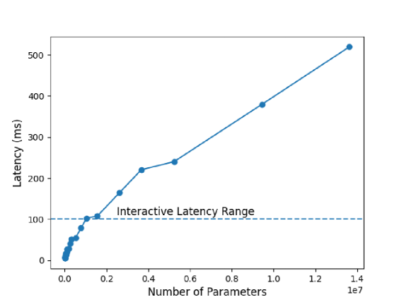
Figure 1: Inference latency of GNNs with varying model sizes on the Flickr Zeng et al. (2020) dataset on a standard GCN model architecture with increasing embedding dimension. All tests were run on a Tesla V100 GPU.

Due to this limitation, large GNNs need to be compressed into smaller GNNs for latency-sensitive applications such as real-time recommendation (Liu et al., 2022a), visual question answering (Senior et al., 2023), image search (Formal et al., 2020), and real-time spam detection (Li et al., 2019).

1.1 Knowledge Distillation

Knowledge Distillation (KD) is a common compression technique that uses a teacher model to supervise the training of a smaller student model (Hinton et al., 2015). While the original KD method can be applied to GNNs, it does not take into account any information about node connectivity. GraphAKD (He et al., 2022), LSP (Yang et al., 2021), and G-CRD (Joshi et al., 2022) are GNN-specific knowledge distillation methods that focus on aligning final layer node embeddings by considering node connectivity. However, these methods all consider only the node embeddings at the final layer and do not consider intermediate representations. By just aligning the final node embeddings, the model cannot learn the logic behind leveraging the connectivity of the graph or the inductive biases (Baxter, 2000) contained in the adjacency matrix. Therefore, the student model is effectively just learning a mapping from node attributes to more refined node embeddings. This can lead to suboptimal test generalization when the model encounters previously unseen data.

Objective: Our goal is to achieve better generalization on out-of-distribution data, measured by accuracy @ various compression rates, by considering intermediate node embeddings and taking into account more of the inductive biases that GNNs contain.

1.2 Attention-Based Knowledge Distillation

To improve accuracy over SOTA, we must consider some of the inductive biases that other methods overlook - the connectivity of the input graph. We observe that for the vast majority of GNN architectures, the $k^{th}$ layer of a GNN computes node embeddings by aggregating information from each node’s $k$-hop neighborhood. Therefore, each layer contains its own inductive bias. As other KD methods consider only the node embeddings at the last layer of the teacher and student networks, they do not leverage all the inductive biases present in the network. However, one obvious challenge that is present in aligning intermediate node embeddings is that teacher and student networks will likely have a different number of hidden layers. As a result, there is no 1-1 correspondence between teacher and student layers and no way to easily figure out which teacher node embeddings should be aligned with which student node embeddings.

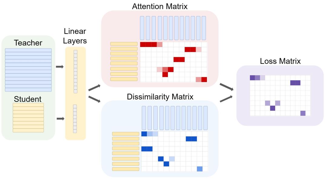
Figure 2: ABKD generates an attention map using a trainable attention mechanism and a dissimilarity map using a trainable subspace projection. The loss matrix is an element-wise multiplication of the attention matrix and the dissimilarity matrix.

To tackle these challenges, we propose Attention-Based Knowledge Distillation (ABKD). We use a trainable attention mechanism to learn which teacher-student pairs are the most important to align. We also utilize trainable projections into a common ABKD embedding space for teacher and student hidden layers. By aligning across intermediate layers, the student learns how to use the adjacency matrix to construct node embeddings instead of just learning a mapping from the node attributes to the final layer node embeddings (Figure 2).

1.3 Our Contributions

Our contributions are summarized as the following:

1. We design Attention-Based Knowledge Distillation (ABKD), a novel knowledge distillation approach for GNNs that incorporates the intermediate feature maps from every layer in both the teacher and student networks. This approach can be utilized to train teacher and student networks of any architectural configuration.

2. We create an automatic feature linking mechanism using attention to identify which teacher-student layer pairs are the most important, which we then use to closely align their feature maps.

3. Our approach broadly improves the test accuracy of student networks over a large range of compression ratios.

4. We comprehensively test our approach on several datasets using different model architectures including GCNs (Kipf & Welling, 2016), RGCNs (Schlichtkrull et al., 2017) and GraphSAGE (Hamilton et al., 2017). We also test on several large datasets that are carefully curated to evaluate out-of-distribution generalization such as OGBN-Mag (Wang et al., 2020) and OGBN-Arxiv (Wang et al., 2020).

2 Related Work

Knowledge Distillation KD for GNNs is a relatively niche field that has expanded over the last three years with the work of LSP (Yang et al., 2021). In this work, the authors attempt to align node embeddings between the student and teacher networks by maximizing the similarity between embeddings that share edges. As only node embeddings between edges are aligned, this KD method only preserves local topology. Joshi et al. (2022) extend LSP and propose two different KD algorithms: Global Structure Preserving Distillation (GSP) and Global Contrastive Representation Distillation (G-CRD). GSP extends LSP by considering all pairwise similarities among node features, not just pairwise similarities between nodes connected by edges. The authors also propose G-CRD which aims to implicitly preserve global topology by aligning the student and teacher node feature vectors via contrastive learning (van den Oord et al., 2018). Another work introduces graph adversarial knowledge distillation (GraphAKD), which trains the student model as a generator network and a discriminator network to distinguish between the predictions of the student and teacher models (He et al., 2022). Another work, GeometricKD forces the number of teacher and student hidden layers to be the same to study the impact of a student network operating on a smaller graph than the teacher (Yang et al., 2023).

With the exception of GeometricKD, these works all consider the node embeddings at the final layer of the teacher and student network and aim to align those embeddings with one another in various ways. GeometricKD constrains the student and teacher networks to have the same number of layers, and it aligns the node embedding of teacher layer $i$ with student layer $i$, thus forming a 1-1 correspondence between the layers, which makes it inflexible to all student and teacher configurations. There have been several KD approaches that have been applied to CNNs that the GNN community has tried to adapt to GNNs with poor results, namely Fitnets (Romero et al., 2015) and attention transfer (Zagoruyko & Komodakis, 2016). These methods both compute a distance metric such as mean-squared error between the last layer node embeddings of the student and teacher network and do not take into account the adjacency matrix.

Using attention to find similarities across student and teacher layers is a concept explored in CNNs Ji et al. (2021). However, this work’s ideas cannot be applied to GNNs because the operations it uses to compare student and teacher features do not apply to GNNs. GNNs need special consideration in this regard over CNNs due to the non-spatial and unstructured form of graph data.

Compression: Other common techniques for GNN compression include quantization and pruning. Quantization techniques differ for GNNs when compared to other deep neural networks because of unique sources of error, such as inaccurate gradient estimates, that arise due to the unstructured nature of GNNs (Tailor et al., 2021). To account for inaccurate gradient estimates, DegreeQuant, protects some number of nodes in every training iteration from lower precision training and utilizes full precision training for those nodes (Tailor et al., 2021). Other approaches consider the structure of the graph in their calculations to implicitly avoid GNN-specific sources of error (Feng et al., 2020; Bahri et al., 2021).

Pruning techniques, which involve compressing networks by selectively deleting learned parameters, have also been applied to GNNs. These techniques involve applying strategies that have worked for other deep networks and using them to identify the most important channels for output activation (Chen et al., 2021b) (Zhou et al., 2021a). One approach also works to dynamically prune during execution (Chen et al., 2021a).

Method	Number of Layers Considered
GraphAKD	$1$
G-CRD	$1$
Fitnets	$1$
LSP	$1$
ABKD	All

Table 1: Comparison of Attention-Based Knowledge Distillation with other Knowledge Distillation approaches.

3 Proposed Approach

3.1 Intuition and Mathematical Foundations

In this section, we first discuss the intuition behind ABKD and introduce some of the mathematical definitions needed to explain it thoroughly.

3.1.1 SoftKD Intuition

In SoftKD (Hinton et al., 2015), we compute two different losses. The first, $H(s_{p},y)$, is a cross-entropy loss between the output student probability distribution and the ground truth labels. The other, $H(s_{p},t_{p})$, is a cross-entropy loss between the output student probability distribution and the output teacher probability distribution. The total loss is defined as:

$$L_{KD}=H(s_{p},y)+\alpha H(s_{p},t_{p})$$ (1)

Here, $\alpha$ is a hyper-parameter controlling how much the KD loss affects the total loss. The goal is to align the output student probability distribution with the output teacher probability distribution. The higher $H(s_{p},t_{p})$ is, the less aligned the student and teacher output probability distributions are.

3.1.2 ABKD Intuition

Similarly, with ABKD, we want to incorporate this intuition of alignment. However, we want to go further than just aligning the final output - we want to align the outputs at the intermediate layers, as the intermediate layers contain inductive biases that are not present in just the final layers. As one of our goals with ABKD is to work with any combination of teacher and student architectural configurations, this presents one significant challenge: Teacher and student networks will likely have a different number of hidden layers, which means there is no 1-1 correspondence between teacher and student layers.

ABKD solves this problem by identifying which teacher-student layer pairs are the most important to align via an attention mechanism. This mechanism works with any arbitrary number of teacher layers and student layers, which makes this approach amenable to any arbitrary teacher-student configuration. ABKD also uses a reprojection technique to account for the student and teacher networks having different hidden dimensions. The output of each hidden layer for both the teacher and student networks is projected into a standardized embedding dimension, which ensures that we can work with student and teacher networks of any embedding dimension. As each layer represents its own semantic information, an important challenge that we faced was to ensure that each layer’s feature map was not smoothed out by a single projection matrix. To this end, we use separate trainable linear layers for each hidden layer in both the teacher and student networks, in order to ensure that we don’t lose out on any valuable semantic information in the hidden layers.

These trainable linear layers help us construct the two key components of ABKD, which are the attention map and the dissimilarity map. At a high level, the attention map tells us how important each teacher-student layer pair is, while the dissimilarity map tells us how distant the feature maps of each teacher-student layer pair are. The teacher-student layer pairs with higher attention scores are deemed as more important, and ABKD focuses on reducing their dissimilarity scores during training.

3.1.3 Mathematical Foundation

Without loss of generality, we will consider distilling a general Graph Convolution Network (GCN) (Kipf & Welling, 2016), in which the output of the $l^{th}$ layer is

$$H^{l}=\sigma(\hat{A}H_{l-1}W_{l})$$ (2)

Here, $\sigma$ is an activation function and $\hat{A}$ is the normalized adjacency matrix, $\hat{A}=D^{-\frac{1}{2}}AD^{-\frac{1}{2}}$, where $D$ is the diagonal degree matrix. $H^{l-1}\in R^{n\times d}$ represents the output of the last hidden layer and $W^{l}\in R^{d\times d}$ represents the trainable weights of the current layer.

Consider two different tensors $T\in R^{T_{l}\times n\times d_{t}}$ and $S\in R^{S_{l}\times n\times d_{s}}$. $T_{l}$ and $S_{l}$ represent the number of layers in the teacher and student networks respectively. $n$ represents the number of nodes in the graph that is being trained on and $d_{t}$ and $d_{s}$ represents the dimensionality of the teacher and student networks, respectively. $T$ and $S$ represent the calculated layer maps before activation is applied at every layer for the teacher and student networks, respectively.

3.2 ABKD

3.2.1 Attention Scores

The first step of ABKD is to generate $A\in R^{T_{l}\times S_{l}}$. $A_{ij}$ will represent an "importance" score for the layer pair consisting of teacher layer $i$ and student layer $j$. We take the average of the feature maps along the node dimension to compute a mean node feature for every layer in both the teacher and student networks. Call these tensors $T_{a}\in R^{T_{l}\times d_{t}}$ and $S_{a}\in R^{S_{l}\times d_{s}}$. Then, we pass each layer in $T_{a}$ through its own linear layer to create $T_{p}\in R^{T_{l}\times d_{a}}$, where $d_{a}$ is the embedding dimension of ABKD. Similarly, we create $S_{p}\in R^{S_{l}\times d_{a}}$. We can finally generate $A$ in the following manner:

$$A=softmax(\frac{T_{p}S_{p}^{T}}{\sqrt{d_{a}}})$$ (3)

3.2.2 Dissimilarity Scores

The next step is to compute a pairwise dissimilarity score for each teacher-student layer pair. Again, we project the features into $d_{a}$. For calculating the attention scores, we averaged over the node dimension before projecting, as our goal was to identify important layers. When calculating the pairwise dissimilarity, we want to incorporate the per-node embeddings. So, we use a separate set of projection matrices. We use $P_{t}\in R^{d_{t}\times d_{a}}$ and $P_{s}\in R^{d_{s}\times d_{a}}$ to represent the projections.

However, distance metrics are less semantically valuable if $d_{a}$ is high. To alleviate this problem, we define a trainable matrix $P\in R^{d_{a}\times d_{a}}$ to project all vectors into the subspace defined by the column space of $P$. Since the cardinality of the subspace defined by the column space of $P$ will be smaller than or equal to the cardinality of $R^{d_{a}}$, distance metrics within the subspace will be more valuable on average compared to distance metrics in $R^{d_{a}}$.

The final step is to average over the embedding dimension and then produce $D\in R^{T_{l}\times S_{l}}$, which gives dissimilarity scores for each teacher-student layer pair. For calculating the dissimilarity, we experiment with Euclidean and cosine distance, but Euclidean distance generally tends to perform better. The dissimilarity score for a layer pair $(i,j)$ can be represented as:

$$D_{ij}=||(T_{i}P_{t}-S_{j}P_{s})P\frac{\mathds{1}_{d_{a}}}{d_{a}}||^{2}_{2}$$ (4)

where $\mathds{1}_{d_{a}}$ is a vector of $1$s in $R^{d_{a}}$.

3.2.3 Final Loss Calculation

To produce the final loss matrix, we element-wise multiply $A$ and $D$ and then take the row-wise mean to produce a single number that represents the ABKD loss.

$$L_{abkd}=(\mathds{1}_{T_{l}})^{T}(A\odot D)(\frac{\mathds{1}_{S_{l}}}{S_{l}})$$ (5)

The final loss is calculated as

$$L=H(s_{p},y)+\beta L_{abkd}$$ (6)

There is one important theorem to consider that proves $L_{abkd}$ distills valuable knowledge from the teacher network to the student network.

Theorem 1: Consider a teacher layer $i$ and a student layer $j$ such that $j<i$. Consider the weight $W_{j}^{s}$ which is the associated weight for the $j^{th}$ layer of the student network. The weight update for $W_{j}^{s}$ will be affected by $W_{i}^{t}$, which are the weights for the $i^{th}$ layer of the teacher network.

Proof: To calculate the weight update, we have to first formulate a loss for the layer pair $(i,j)$. By adapting equation 5 to a specific element in the loss matrix, we get:

$$L_{ij} \sim(\frac{\mathds{1}_{n}}{n})^{T}(T^{p}_{i}(W_{j}^{ps})^{T})(W_{j}^{s})^{T}((H^{s}_{j-1})^{T}\hat{A}^{T}))\frac{\mathds{1}_{n}}{n}*D_{ij}$$

$$T^{p}_{i} =\hat{A}H_{i-1}^{t}W^{t}_{i}W_{i}^{pt}$$

where $W_{i}^{pt}$ and $W_{j}^{ps}$ represent the projection matrices used to calculate the attention score.

Assuming that our weight updates are performed by gradient descent, to calculate the weight update for $W_{j}^{s}$ due to $L_{ij}$, we have to first calculate $\frac{\partial L_{ij}}{\partial W_{j}^{s}}\in R^{d_{s}\times d_{s}}$:

$$\frac{\partial L_{ij}}{\partial W_{j}^{s}}=\frac{\partial A_{ij}}{W_{j}^{s}}D_{ij}+\frac{\partial D_{ij}}{W_{j}^{s}}A_{ij}$$ (7)

We focus on the first term and obtain the result:

$$\frac{\partial A_{ij}}{\partial W_{j}^{s}}\sim((H_{j-1}^{s})^{T}\hat{A}^{T}(\frac{\mathds{1}_{n}}{n}))((\frac{\mathds{1}_{n}}{n})^{T}T_{i}^{p}(W_{j}^{ps})^{T})$$ (8)

It is apparent that as $\frac{\partial A_{ij}}{\partial W_{j}^{s}}$ contains the term $T^{p}_{i}=\hat{A}H_{i-1}^{t}W^{t}_{i}W_{i}^{pt}$, the weight update will reflect terms from the $i^{th}$ teacher layer. This theorem goes to show that even though student layer $j$ is responsible for aggregating information for every node from its $j$-hop neighborhood, its weights collect knowledge from teacher layer $i$ - knowledge that would be unavailable to student layer $j$ using any of the other GNN KD approaches.

An important follow-up observation is that the loss for a teacher-student layer pair will be higher if the pair is deemed as more important and if their projected feature maps have a high dissimilarity score ($D_{ij}>0.5)$, which indicates that they aren’t closely aligned.

To verify this observation, consider an arbitrary teacher layer $i$ and an arbitrary student layer $j$. Consider $A_{ij}$. If the pair $(i,j)$ is deemed important, $A_{ij}$ will be high. Now consider $D_{ij}$. If the pair $(i,j)$ is not closely aligned, then $D_{ij}$ will be high. As $L_{ij}=A_{ij}*D_{ij}$, if both $A_{ij}$ and $D_{ij}$ are high, then $L_{ij}$ will also be high, hence proving that the loss is high for important but misaligned layer pairs.

4 Experiments

Figure 3: Accuracy vs. Compression Ratio: A comparison of KD methods applied to student models of different sizes trained on the OGBN-Mag dataset. The teacher model was the same model as the one described in table 3. The student model was a two-layer RGCN and we varied the embedding dimension from 16 - 512 to induce this Pareto frontier. The y-axis represents the test accuracy of the final trained models.

Dataset	OGBN-Mag	OGBN-Arxiv
Teacher	RGCN (3L-512H-5.5M)	GAT (3L-750H-1.4M)
Student	RGCN (2L-32H-170K)	GS (2L-256H-87K)
Teacher	$49.80$	$74.20$
Student	$44.23\pm 0.47$	$70.87\pm 0.58$
Fitnet	$44.87\pm 0.84$	$71.32\pm 0.32$
AT	$43.87\pm 0.67$	$71.04\pm 0.48$
LSP	$45.21\pm 0.54$	$71.47\pm 0.45$
GSP	$44.97\pm 0.58$	$71.97\pm 0.64$
G-CRD	$45.42\pm 0.43$	$71.87\pm 0.56$
ABKD	$\mathbf{47.21\pm 0.32}$	$\mathbf{73.25\pm 0.56}$
Ratio	$32.3\times$	$16.1\times$

Table 2: Average accuracies over five trials for the OGBN-Mag and OGBN-Arxiv Datasets. The teacher network was kept constant while the different distillation methods were applied to student networks that were initialized from the same set of weights. GS means GraphSAGE.

4.1 Experimental Setup

For our main experiments, we test ABKD on two difficult datasets OGBN-Mag and OGBN-Arxiv (Wang et al., 2020). These datasets employ temporal splitting to create validation and test sets that can assess a model’s ability to generalize on out-of-distribution data (Hu et al., 2020). For OGBN-Mag, we run experiments using RGCN (Schlichtkrull et al., 2017) as the teacher and student models, and for OGBN-Arxiv, we run experiments using GAT (Veličković et al., 2018) as the teacher model and GraphSAGE (Hamilton et al., 2017) as the student model. This allows us to evaluate the effectiveness of ABKD for different GNN architectures. It also allows us to assess if ABKD can distill information between different types of GNN architectures. In our experiments, we keep the teacher model architecture and weights fixed and only modify the size of the student network. Each distillation method starts from the same set of weights and trains for the same number of epochs across 5 runs. For our baselines, we consider LSP (Yang et al., 2021), GSP (Joshi et al., 2022), G-CRD (Joshi et al., 2022), Fitnet (Romero et al., 2015), and Attention Transfer (Zagoruyko & Komodakis, 2016). We ran all experiments on a Tesla V100 GPU.

4.2 Experimental Results

Out-Of-Distribution Evaluation As evidenced by our results in Table 2, we are able to outperform SOTA in several different compression settings on OGBN-Mag and OGBN-Arxiv. We show improvements of over $1.79\%$ and $1.38\%$ with compression ratios of $32.3\times$ and $16.1\times$ on OGBN-Mag and OGBN-Arxiv respectively. As these datasets are intended to evaluate out-of-distribution generalization, our results empirically prove that ABKD can train student models that generalize better than other KD approaches.

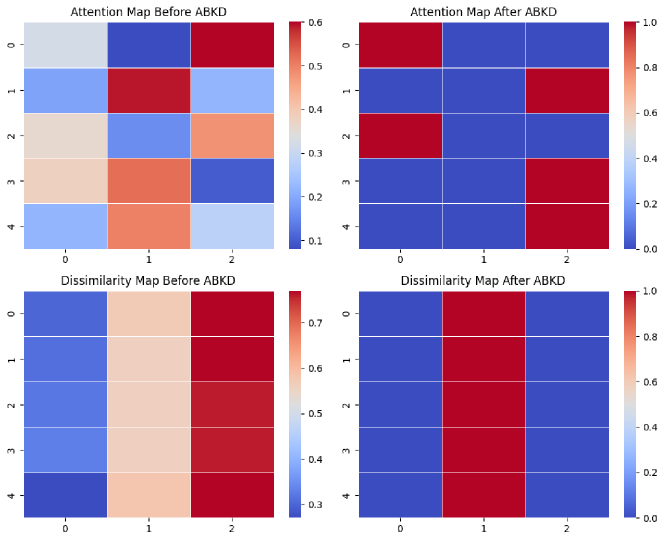
Figure 4: Attention and Dissimilarity maps before and after training with ABKD. Cooler colors refer to lower scores and warmer colors correspond to higher scores.

ABKD aligns intermediate embeddings: To empirically prove that ABKD actually aligns intermediate embeddings based on the attention matrix, we visualize the before and after training attention and dissimilarity maps in figure 4. We train on OGBN-Mag and use a deeper teacher network of 5 layers and a hidden dimension of 512. The student network has 3 layers and a hidden dimension of 32. Our results show that dissimilarity scores are low where the attention scores are high and vice versa. This is in line with the intuition that we constructed in 3.2.3.

Dataset	Cora	Citeseer	Pubmed	NELL
Teacher	GCNII (64L-64H)	GCNII (64L-64H)	GCNII (64L-64H)	GCNII (64L-64H)
Student	GCNII (4L-4H)	GCNII (4L-4H)	GCNII (4L-4H)	GCNII (4L-4H)
Teacher	$88.40$	$77.33$	$89.78$	$95.55$
Student	$74.22\pm 1.32$	$68.14\pm 1.45$	$88.66\pm 0.87$	$85.20\pm 0.75$
LSP	$75.18\pm 1.45$	$70.43\pm 1.32$	$89.01\pm 1.73$	$85.20\pm 1.32$
GSP	$78.32\pm 1.21$	$69.43\pm 0.87$	$89.13\pm 1.05$	$86.13\pm 1.47$
G-CRD	$83.35\pm 1.32$	$71.42\pm 1.21$	$89.73\pm 1.05$	$88.61\pm 1.01$
ABKD	$\mathbf{84.27\pm 1.48}$	$\mathbf{71.96\pm 0.87}$	$\mathbf{89.87\pm 0.45}$	$\mathbf{91.83\pm 0.74}$
# Parameters	$5835$	$14910$	$2083$	$22686$
Ratio	$60.7\times$	$33.5\times$	$141.3\times$	$27.7\times$

Table 3: Average accuracies over several trials for a variety of datasets, using GCNII. The results are based on the average of five trials, with each distillation method applied to the same set of student weights.

Deep GNNs: We also test ABKD on deep GNN architectures. While most GNN architectures are shallow due to the problem of over-smoothing, there are some approaches that alleviate this issue, allowing for deep GNN architectures. One of these approaches is GCNII (Chen et al., 2020). We test on Cora (Mccallum et al., 2000), Citeseer (Sen et al., 2008), Pubmed (Namata et al., 2012) and NELL (Carlson et al., 2010). Table 3 shows that ABKD is able to distill these deep GCNIIs into shallower GCNIIs with higher accuracy compared to other distillation methods in high compression settings. While currently, most GNN use cases require shallow GNNs, this could be useful for future applications that require deeper GNNs.

Improved Weight Initialization for Highly Compressed Networks: We find that for smaller datasets, information from the teacher network is mainly distilled into one layer of the student network, as shown in Figure 5. Our hypothesis for this occurrence is that smaller datasets are not very complex and one layer is sufficient for learning most of the patterns. Through experimentation, we prove that when we initialize a one-layer network from the weights of this particular layer, we get improved accuracy compared to random initialization, as shown in Table 4.

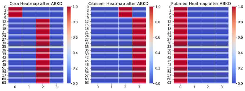
Figure 5: Attention maps for Cora, Citeseer, and Pubmed. Each color in the heatmap represents the importance score associated with that teacher-student layer pair. Warmer colors mean higher important scores. It seems apparent that most of the knowledge from the teacher layers is distilled into one student layer.

Dataset	Initialized	Random Init	No Training
Cora	$80.29$	$73.58$	$65.36$
Citeseer	$70.12$	$68.12$	$54.20$
Pubmed	$88.76$	$86.03$	$72.90$

Table 4: Results for weight initialization experiment. Experimental details can be found in the appendix.

Dataset	OGBN-Mag	OGBN-Arxiv
Student	$44.46\pm 0.54$	$71.27\pm 0.48$
ABKD	$\mathbf{47.46\pm 0.45}$	$\mathbf{73.18\pm 0.56}$
Modified ABKD	$46.56\pm 0.60$	$71.89\pm 0.87$

Table 5: Ablation study comparing modified ABKD that only considers aligning the last layer node embeddings with ABKD that considers intermediate layer node embeddings. The teacher and student models are the same as the ones in Table 2.

4.3 Ablation Studies

Aligning Intermediate Layers is Important: To prove that the aligning of intermediate layers is necessary for superior performance, we experiment with a variant of ABKD, which we call modified ABKD, where we set $A\in R^{T_{l}\times S_{l}}$ to all zeros, but we set the bottom right value to 1. This indicates that we are only interested in the dissimilarity between the last layer node embeddings of the teacher and student models. The results in table 5, prove that we gain accuracy by considering the outputs of intermediate layers for both teacher and student models. In this experiment, we start from the same set of initialized weights for both the ABKD and modified ABKD approaches.

Improvements due to Subspace Projection: In our approach, we introduced the concept of subspace projection as an alleviation to high dimensional embedding spaces. While it is not needed for ABKD to work, it does improve our results as the learned subspace projection matrix tends to be of lower rank than the embedding dimension. This indicates that we can project our feature maps into subspaces smaller than $R^{d_{a}}$, which increases the semantic value of the dissimilarity scores.

One Linear Layer Per Hidden Layer Is Necessary: In our approach, we mention that each hidden teacher and student layer is assigned its own linear layer for projection into $d_{a}$. This is because each layer represents its own $k$-hop neighborhood, and using just one linear layer would prove inadequate in capturing the full spectrum of essential semantic information contained within each layer. We run an experiment in which we use only one linear layer for the teacher and student projections and demonstrate that there is a significant accuracy dropoff compared to using individual linear layers for the projection.

Dataset	Subspace Projection	No Projection
Cora	$84.27\pm 1.32$	$83.78\pm 1.25$
Citeseer	$71.96\pm 0.83$	$71.46\pm 1.21$
Pubmed	$89.87\pm 0.87$	$89.03\pm 1.04$
NELL	$91.83\pm 0.85$	$90.98\pm 0.75$
OGBN-Mag	$47.21\pm 0.32$	$46.83\pm 0.45$
OGBN-Arxiv	$73.25\pm 0.56$	$72.87\pm 0.34$

Table 6: Subspace Projection Ablation Results. The teacher and student networks are the same as the ones described in tables 2 and 3.

Dataset	Multiple Linear Layers	One Linear Layer
Cora	$84.27\pm 1.48$	$75.52\pm 1.32$
Citeseer	$71.96\pm 0.87$	$68.86\pm 1.27$
Pubmed	$89.87\pm 0.45$	$88.75\pm 0.64$
NELL	$91.83\pm 0.74$	$85.38\pm 0.68$
OGBN-Mag	$47.21\pm 0.32$	$44.67\pm 0.54$
OGBN-Arxiv	$73.25\pm 0.56$	$71.23\pm 0.47$

Table 7: Linear Layer Ablation Results. The teacher and student networks are the same as the ones described in tables 2 and 3.

5 Conclusion

Graph Neural Networks (GNNs) have increased in complexity in recent years, owing to the rapidly increasing size of graph datasets. This increase in complexity poses a problem for latency-sensitive applications such as real-time recommendation and real-time spam detection, as GNN model sizes do not scale well with latency. To address this predicament, we propose an innovative solution known as Attention-Based Knowledge Distillation (ABKD). ABKD employs an attention-based feature linking mechanism to identify important intermediate teacher-student layer pairs and focuses on aligning the node embeddings of those pairs. This knowledge distillation approach broadly outperforms SOTA GNN-specific KD approaches over a wide variety of compression settings. It also works with both deep and shallow networks as proven by our experiments and performs well with several different types of GNN architectures. On average, we achieve a $1.79\%$ increase in accuracy with a $32.3\times$ compression ratio on OGBN-Mag, a large graph dataset, compared to state-of-the-art approaches.

Supplementary Materials

Appendix A Summary of Notations

In Section 3, we mathematically describe how ABKD generates the attention matrix, $A$, and the dissimilarity matrix, $D$, which is then used to calculate $L_{\texttt{ABKD}}$. In Table 8, we provide a summary of all the mathematical notation used to describe ABKD.

Term	Definition
$A_{ij}$	Attention score for the teacher-student layer pair $(i,j)$
$D_{ij}$	Dissimilarity score for the teacher-student layer pair $(i,j)$
$\mathds{1}_{n}\in R^{n}$	Vector of ones in $R^{n}$
$T_{i}\in R^{n\times d_{t}}$	The output of the $i^{th}$ layer in the teacher network.
$S_{j}\in R^{n\times d_{s}}$	The output of the $j^{th}$ layer in the student network
$T_{i}^{p}\in R^{d_{a}}$	The projected output of the $i^{th}$ student layer after taking the node-wise mean
$W_{i}^{pt}\in R^{d_{t}\times d_{a}}$	The learnable $i^{th}$ projection matrix for the teacher network
$W_{j}^{ps}\in R^{d_{s}\times d_{a}}$	The learnable $j^{th}$ projection matrix for the student network
$P_{t}\in R^{d_{t}\times d_{a}}$	The learnable projection matrix for the teacher network; used to calculate the dissimilarity score
$P_{s}\in R^{d_{s}\times d_{a}}$	The learnable projection matrix for the student network; used to calculate the dissimilarity score
$P\in R^{d_{a}\times d_{a}}$	The learnable subspace projection matrix. Shared between the student and teacher networks

Table 8: Summary of mathematical notation used in Section 3.

Appendix B Further Experimental Discussion and Ablations

B.1 Dataset and Teacher Network Information

Tables 6 and 7 provide information on the datasets used in Section 4 and the corresponding teacher networks employed to supervise the training of various student networks during our experiments.

	# of Nodes	# of Edges	# of Features	# of Classes
Cora	2,708	10,556	1,433	7
Citeseer	3,327	9,104	3,703	6
Pubmed	19,717	88,648	500	3
OGBN-Mag	1,939,743	21,111,007	128	349
OGBN-Arxiv	169,343	1,166,243	128	40

Table 9: Specification of evaluated datasets.

B.2 Weight Initialization Experiment Details

In Section 4.2, we present the results of an experiment in which we instantiate a one-layer network from the attention maps generated by ABKD. The first step of this experiment is to run ABKD on a student network of any arbitrary size and then generate the attention map, $A\in R^{T_{l}\times S_{l}}$. The next step is to use a row-wise argmax and find the student layer that has the most information distilled down to it. For example, in Figure 5, the selected layer for Cora would be the third student layer (index 2 in the figure). We then proceed to instantiate a new one-layer network and copy over the weights from the identified layer from $A$. We then evaluate this new network on the test set and report the results in column 3 of Table 4. The first column of Table 4 represents the accuracies that we obtain after we train the new one-layer network for $1200$ epochs; we compare this result to the accuracy obtained from training a one-layer network from random initialization, which we report in the second column of Table 4.

B.3 Hyperparameter Ablation Studies

There are two main hyperparameters that need to be tuned when training ABKD: the loss coefficient, $\beta$, and the ABKD embedding dimension, $d_{a}$. We present the test accuracies across various values for $\beta$ and $d_{a}$ in Tables 10 and 11. These results show that a lower $\beta$ and a higher $d_{a}$ tend to produce slightly better results. For all of our experiments, we used a $\beta$ of $10$ and a $d_{a}$ of 256 for this reason.

Dataset	$\beta=1$	$\beta=10$	$\beta=20$	$\beta=50$
Cora	$86.92$	$84.71$	$86.19$	$85.64$
Citeseer	$73.20$	$74.33$	$71.82$	$69.82$
Pubmed	$89.03$	$89.97$	$88.32$	$88.56$
NELL	$90.86$	$88.73$	$90.14$	$91.32$

Table 10: Ablation results for $\beta$.

Dataset	$d_{a}=64$	$d_{a}=128$	$d_{a}=256$	$d_{a}=512$
Cora	$87.45$	$87.11$	$86.92$	$86.37$
Citeseer	$72.07$	$72.52$	$73.12$	$74.62$
Pubmed	$89.58$	$89.58$	$89.33$	$89.12$
NELL	$89.73$	$90.12$	$90.73$	$91.14$

Table 11: Ablation results for $d_{a}$.

Dataset	Euclidean Distance	Cosine Distance
Cora	$87.33$	$82.81$
Citeseer	$73.43$	$70.98$
Pubmed	$89.58$	$87.32$
NELL	$91.24$	$85.66$

Table 12: Test accuracies when using Euclidean distance vs. cosine distance for computing $D$.

In Section 3.2.2, we mention that we use a Euclidean distance metric instead of a cosine distance metric to generate the dissimilarity matrix, $D$. We present the results of this ablation in Table 12. As cosine distance disregards the magnitude of the vectors, we hypothesize that the magnitude of the hidden layer outputs is important. Furthermore, as Euclidean distance takes into account the magnitude of the hidden layer outputs, this is likely why it performs significantly better than cosine distance.

References

- Bahri et al. (2021) Mehdi Bahri, Gaétan Bahl, and Stefanos Zafeiriou. Binary graph neural networks, 2021.
- Baxter (2000) J. Baxter. A model of inductive bias learning. Journal of Artificial Intelligence Research, 12:149–198, mar 2000. doi: 10.1613/jair.731. URL https://doi.org/10.1613%2Fjair.731.
- Carlson et al. (2010) Andrew Carlson, Justin Betteridge, Bryan Kisiel, Burr Settles, Estevam Hruschka, and Tom Mitchell. Toward an architecture for never-ending language learning. Proceedings of the AAAI Conference on Artificial Intelligence, 24(1):1306–1313, Jul. 2010. doi: 10.1609/aaai.v24i1.7519. URL https://ojs.aaai.org/index.php/AAAI/article/view/7519.
- Chen et al. (2021a) Cen Chen, Kenli Li, Xiaofeng Zou, and Yangfan Li. Dygnn: Algorithm and architecture support of dynamic pruning for graph neural networks. In 2021 58th ACM/IEEE Design Automation Conference (DAC), pp. 1201–1206, 2021a. doi: 10.1109/DAC18074.2021.9586298.
- Chen et al. (2022) Chaoqi Chen, Yushuang Wu, Qiyuan Dai, Hong-Yu Zhou, Mutian Xu, Sibei Yang, Xiaoguang Han, and Yizhou Yu. A survey on graph neural networks and graph transformers in computer vision: A task-oriented perspective, 2022.
- Chen et al. (2020) Ming Chen, Zhewei Wei, Zengfeng Huang, Bolin Ding, and Yaliang Li. Simple and deep graph convolutional networks. CoRR, abs/2007.02133, 2020. URL https://arxiv.org/abs/2007.02133.
- Chen et al. (2021b) Tianlong Chen, Yongduo Sui, Xuxi Chen, Aston Zhang, and Zhangyang Wang. A unified lottery ticket hypothesis for graph neural networks, 2021b.
- Feng et al. (2020) Boyuan Feng, Yuke Wang, Xu Li, Shu Yang, Xueqiao Peng, and Yufei Ding. Sgquant: Squeezing the last bit on graph neural networks with specialized quantization, 2020.
- Formal et al. (2020) Thibault Formal, Stéphane Clinchant, Jean-Michel Renders, Sooyeol Lee, and Geun Hee Cho. Learning to rank images with cross-modal graph convolutions. In Joemon M. Jose, Emine Yilmaz, João Magalhães, Pablo Castells, Nicola Ferro, Mário J. Silva, and Flávio Martins (eds.), Advances in Information Retrieval, pp. 589–604, Cham, 2020. Springer International Publishing. ISBN 978-3-030-45439-5.
- Hamilton et al. (2017) William L. Hamilton, Rex Ying, and Jure Leskovec. Inductive representation learning on large graphs. CoRR, abs/1706.02216, 2017. URL http://arxiv.org/abs/1706.02216.
- Han et al. (2020) Yi Han, Shanika Karunasekera, and Christopher Leckie. Graph neural networks with continual learning for fake news detection from social media, 2020.
- He et al. (2022) Huarui He, Jie Wang, Zhanqiu Zhang, and Feng Wu. Compressing deep graph neural networks via adversarial knowledge distillation, 2022.
- Hinton et al. (2015) Geoffrey Hinton, Oriol Vinyals, and Jeff Dean. Distilling the knowledge in a neural network, 2015.
- Hu et al. (2020) Weihua Hu, Matthias Fey, Marinka Zitnik, Yuxiao Dong, Hongyu Ren, Bowen Liu, Michele Catasta, and Jure Leskovec. Open graph benchmark: Datasets for machine learning on graphs. CoRR, abs/2005.00687, 2020. URL https://arxiv.org/abs/2005.00687.
- Ji et al. (2021) Mingi Ji, Byeongho Heo, and Sungrae Park. Show, attend and distill:knowledge distillation via attention-based feature matching, 2021.
- Joshi et al. (2022) Chaitanya K. Joshi, Fayao Liu, Xu Xun, Jie Lin, and Chuan Sheng Foo. On representation knowledge distillation for graph neural networks. IEEE Transactions on Neural Networks and Learning Systems, pp. 1–12, 2022. doi: 10.1109/tnnls.2022.3223018. URL https://doi.org/10.1109%2Ftnnls.2022.3223018.
- Kipf & Welling (2016) Thomas N. Kipf and Max Welling. Semi-supervised classification with graph convolutional networks. CoRR, abs/1609.02907, 2016. URL http://arxiv.org/abs/1609.02907.
- Li et al. (2019) Ao Li, Zhou Qin, Runshi Liu, Yiqun Yang, and Dong Li. Spam review detection with graph convolutional networks. In Proceedings of the 28th ACM International Conference on Information and Knowledge Management, CIKM ’19, pp. 2703–2711, New York, NY, USA, 2019. Association for Computing Machinery. ISBN 9781450369763. doi: 10.1145/3357384.3357820. URL https://doi.org/10.1145/3357384.3357820.
- Liu et al. (2022a) Zhuoran Liu, Leqi Zou, Xuan Zou, Caihua Wang, Biao Zhang, Da Tang, Bolin Zhu, Yijie Zhu, Peng Wu, Ke Wang, and Youlong Cheng. Monolith: Real time recommendation system with collisionless embedding table, 2022a.
- Liu et al. (2022b) Zirui Liu, Kaixiong Zhou, Fan Yang, Li Li, Rui Chen, and Xia Hu. EXACT: Scalable graph neural networks training via extreme activation compression. In International Conference on Learning Representations, 2022b. URL https://openreview.net/forum?id=vkaMaq95_rX.
- Mccallum et al. (2000) Andrew Mccallum, Kamal Nigam, and Jason Rennie. Automating the construction of internet portals. 03 2000.
- Namata et al. (2012) Galileo Namata, Ben London, Lise Getoor, and Bert Huang. Query-driven active surveying for collective classification. 2012.
- Que et al. (2023) Zhiqiang Que, Hongxiang Fan, Marcus Loo, He Li, Michaela Blott, Maurizio Pierini, Alexander D. Tapper, and Wayne Luk. Ll-gnn: Low latency graph neural networks on fpgas for high energy physics, 2023.
- Romero et al. (2015) Adriana Romero, Nicolas Ballas, Samira Ebrahimi Kahou, Antoine Chassang, Carlo Gatta, and Yoshua Bengio. Fitnets: Hints for thin deep nets, 2015.
- Schlichtkrull et al. (2017) Michael Schlichtkrull, Thomas N. Kipf, Peter Bloem, Rianne van den Berg, Ivan Titov, and Max Welling. Modeling relational data with graph convolutional networks, 2017.
- Sen et al. (2008) Prithviraj Sen, Galileo Namata, Mustafa Bilgic, Lise Getoor, Brian Galligher, and Tina Eliassi-Rad. Collective classification in network data. AI Magazine, 29(3):93, Sep. 2008. doi: 10.1609/aimag.v29i3.2157. URL https://ojs.aaai.org/index.php/aimagazine/article/view/2157.
- Senior et al. (2023) Henry Senior, Gregory Slabaugh, Shanxin Yuan, and Luca Rossi. Graph neural networks in vision-language image understanding: A survey, 2023.
- Tailor et al. (2021) Shyam A. Tailor, Javier Fernandez-Marques, and Nicholas D. Lane. Degree-quant: Quantization-aware training for graph neural networks, 2021.
- Tan et al. (2023) Zeyuan Tan, Xiulong Yuan, Congjie He, Man-Kit Sit, Guo Li, Xiaoze Liu, Baole Ai, Kai Zeng, Peter Pietzuch, and Luo Mai. Quiver: Supporting gpus for low-latency, high-throughput gnn serving with workload awareness, 2023.
- van den Oord et al. (2018) Aäron van den Oord, Yazhe Li, and Oriol Vinyals. Representation learning with contrastive predictive coding. CoRR, abs/1807.03748, 2018. URL http://arxiv.org/abs/1807.03748.
- Veličković et al. (2018) Petar Veličković, Guillem Cucurull, Arantxa Casanova, Adriana Romero, Pietro Liò, and Yoshua Bengio. Graph attention networks, 2018.
- Wang et al. (2020) Kuansan Wang, Zhihong Shen, Chiyuan Huang, Chieh-Han Wu, Yuxiao Dong, and Anshul Kanakia. Microsoft Academic Graph: When experts are not enough. Quantitative Science Studies, 1(1):396–413, 02 2020. ISSN 2641-3337. doi: 10.1162/qss_a_00021. URL https://doi.org/10.1162/qss_a_00021.
- Yang et al. (2023) Chenxiao Yang, Qitian Wu, and Junchi Yan. Geometric knowledge distillation: Topology compression for graph neural networks, 2023.
- Yang et al. (2021) Yiding Yang, Jiayan Qiu, Mingli Song, Dacheng Tao, and Xinchao Wang. Distilling knowledge from graph convolutional networks, 2021.
- Ying et al. (2018) Rex Ying, Ruining He, Kaifeng Chen, Pong Eksombatchai, William L. Hamilton, and Jure Leskovec. Graph convolutional neural networks for web-scale recommender systems. CoRR, abs/1806.01973, 2018. URL http://arxiv.org/abs/1806.01973.
- Zagoruyko & Komodakis (2016) Sergey Zagoruyko and Nikos Komodakis. Paying more attention to attention: Improving the performance of convolutional neural networks via attention transfer. CoRR, abs/1612.03928, 2016. URL http://arxiv.org/abs/1612.03928.
- Zeng et al. (2020) Hanqing Zeng, Hongkuan Zhou, Ajitesh Srivastava, Rajgopal Kannan, and Viktor Prasanna. Graphsaint: Graph sampling based inductive learning method, 2020.
- Zhou et al. (2021a) Hongkuan Zhou, Ajitesh Srivastava, Hanqing Zeng, Rajgopal Kannan, and Viktor Prasanna. Accelerating large scale real-time GNN inference using channel pruning. Proceedings of the VLDB Endowment, 14(9):1597–1605, may 2021a. doi: 10.14778/3461535.3461547. URL https://doi.org/10.14778%2F3461535.3461547.
- Zhou et al. (2021b) Hongkuan Zhou, Ajitesh Srivastava, Hanqing Zeng, Rajgopal Kannan, and Viktor Prasanna. Accelerating large scale real-time gnn inference using channel pruning. arXiv preprint arXiv:2105.04528, 2021b.
- Zitnik & Leskovec (2017) Marinka Zitnik and Jure Leskovec. Predicting multicellular function through multi-layer tissue networks. CoRR, abs/1707.04638, 2017. URL http://arxiv.org/abs/1707.04638.