Online Robust Mean Estimation

Abstract

We study the problem of high-dimensional robust mean estimation in an online setting. Specifically, we consider a scenario where $n$ sensors are measuring some common, ongoing phenomenon. At each time step $t=1,2,\ldots,T$, the $i^{th}$ sensor reports its readings $x^{(i)}_{t}$ for that time step. The algorithm must then commit to its estimate $\mu_{t}$ for the true mean value of the process at time $t$. We assume that most of the sensors observe independent samples from some common distribution $X$, but an $\epsilon$-fraction of them may instead behave maliciously. The algorithm wishes to compute a good approximation $\mu$ to the true mean $\mu^{\ast}:=\mathbf{E}[X]$. We note that if the algorithm is allowed to wait until time $T$ to report its estimate, this reduces to the well-studied problem of robust mean estimation. However, the requirement that our algorithm produces partial estimates as the data is coming in substantially complicates the situation.

We prove two main results about online robust mean estimation in this model. First, if the uncorrupted samples satisfy the standard condition of $(\epsilon,\delta)$-stability, we give an efficient online algorithm that outputs estimates $\mu_{t}$, $t\in[T],$ such that with high probability it holds that $\|\mu-\mu^{\ast}\|_{2}=O(\delta\log(T))$, where $\mu=(\mu_{t})_{t\in[T]}$. We note that this error bound is nearly competitive with the best offline algorithms, which would achieve $\ell_{2}$-error of $O(\delta)$. Our second main result shows that with additional assumptions on the input (most notably that $X$ is a product distribution) there are inefficient algorithms whose error does not depend on $T$ at all.

1 Introduction

1.1 Motivation and Background

One of the most fundamental problems in statistics is that of mean estimation: given a collection of $n$ i.i.d. samples drawn from an unknown distribution $X$ assumed to lie in some known distribution family $\mathcal{F}$, the goal is to output an accurate estimate of the unknown mean $\mu^{\ast}$ of $X$. While this vanilla setting is fairly well understood, it does not capture a number of practically pressing real-world scenarios, where (i) due to modeling issues, the underlying distribution $X$ we sample from does not lie in the known family $\mathcal{F}$ but is only close to it, and (ii) a fraction of the samples are arbitrarily corrupted by malicious users.

The field of robust statistics aims to design estimators that can tolerate up to a constant fraction of corruptions, independent of the data dimensionality [Tuk60, Hub64, HR09]. Classical works in the field have identified the statistical limits of several problems in the robust setting, both in terms of constructing robust estimators and proving information-theoretic lower bounds [Yat85, DL88, DG92, HR09]. However, the early estimators proposed in the statistics literature were not computationally efficient, typically requiring exponential running time in the number of dimensions, see, e.g., [Ber06, HR09].

A relatively recent line of work, originating in computer science [DKK⁺16, LRV16], has developed the field of algorithmic high-dimensional robust statistics, aiming to design estimators that not only attain tight robustness guarantees, but are also efficiently computable. This line of research has provided computationally efficient estimators for a variety of statistical tasks, including mean and covariance estimation, linear regression, and many others, under natural distributional assumptions on the uncorrupted data; see [DK21, DK23] for an overview of this area.

This recent progress notwithstanding, the vast majority of the recent literature on algorithmic robust statistics focuses on the offline setting, where the (corrupted) dataset is given in the input and the goal is to produce a single accurate estimate. For example, in (offline) robust mean estimation, we are given a dataset of $n$ points in $\mathbb{R}^{M}$, an $\epsilon$-fraction of which are corrupted, and the goal is to estimate the mean of the distribution that generated the uncorrupted samples.

The aforementioned offline setting fails to model some commonly arising situations. First, we may need to produce estimations for a series of related statistical tasks that come in sequentially. Second, we are often able to identify the providers of the data. This can be modeled abstractly as follows. Consider the scenario that we have $n$ sensors over which an $\epsilon$-fraction may be hijacked by an adversary or simply malfunctioning. These sensors are collecting information about some common, ongoing stochastic process. In particular, if the stochastic process has $T$ stages, we can model it mathematically as a $T$-dimensional distribution $X$ such that $X_{t}$ encodes the state of the process at time step $t$. Then, at each time step $t$, each uncorrupted sensor give us a report which is an i.i.d. sample from $X_{t}$ and the corrupted ones may give some arbitrary out-of-distribution reports. Our goal is then to compute some statistics related to $X_{t}$ at each time step given the reports received so far. A concrete scenario is described below.

Online Decision Making with User Feedback

A company is trying to deploy a series of new features. Before deployment, a random set of users are selected for trials. After the trial session of each feature ends, the development team needs an estimate of a typical user’s rating to the feature to decide whether it is ready for public deployment. While most feedbacks from the trial users probably do follow a stochastic pattern, some may be significantly “out of distribution”. For example, they may originate from a non-typical user who has special demands or even a fake user account registered by competitors. Ideally, we woudly like to identify these outlier users so as to minimize their total impact to our estimations in the long run.

Indeed, similar scenarios arise whenever we face a sequence of statistical estimation tasks which share the same set of data providers that may not be completely trustworthy. Though the statistical tasks themselves may be independent of each other, the underlying statistical estimation algorithms should not run independently as that will allow adversarial data providers to disturb the outcomes in every estimation task. The more favorable way is always to get rid of the suspicious data providers during early tasks so as to minimize their influence in the future.

At a more philosophical level, we aim at providing a mathematical framework through which one can develop algorithmic ways to establish trust over different information sources over time. Almost on a daily basis we are required to make decisions or judgements based on information collected from different channels, such as social media, television or even gossip. How much we believe a new story we hear may depend upon the degree to which we trust the source (based on our judgement of previous data from that source) and on how consistent the story is with others.

In this work, we make a concrete step in formulating such scenarios. Specifically, we define and study a natural notion of high-dimensional robust mean estimation in the online setting.

Online Robust Mean Estimation: Problem Setup

Throughout this work, we consider the standard strong contamination model.

Definition 1 (Strong Contamination Model).

Given a parameter $0\leq\epsilon<1/2$ and a set $\mathcal{C}$ of $n$ samples, the strong contamination adversary operates as follows. After observing the entire set $\mathcal{C}$, the adversary can remove up to $\epsilon n$ samples from $\mathcal{C}$ and replace them by arbitrary points. The resulting set $\mathcal{X}$ is called an $\epsilon$-corrupted version of $\mathcal{C}$.

We are now ready to define our notion of robust online mean estimation. Intuitively, our goal is to model the scenario where a series of mean estimation tasks need to be completed sequentially, using data collected from a set of sensors over which $\epsilon$-fraction are either hijacked or malfunctioning. In more detail, we introduce the following definition.

Definition 2 (Online Mean Estimation under Strong Contamination).

Given $M,T\in\mathbb{Z}^{+}$, such that $M$ is an integer multiple of $T$, and $0\leq\epsilon<1/2$, let $\mathcal{X}=\{x^{(1)},\cdots,x^{(n)}\}$ be an $\epsilon$-corrupted version of a clean set of i.i.d. samples from a distribution $X$ on $\mathbb{R}^{M}$ with unknown mean $\mu^{*}$. The $M$ coordinates of each datapoint are divided into $T$ batches, each of size $d\stackrel{{\scriptstyle{\mathrm{\footnotesize def}}}}{{=}}M/T$ , i.e., $x^{(i)}$ is the concatenation of $x^{(i)}_{1},\cdots,x^{(i)}_{T}$, where $x^{(i)}_{t}\in\mathbb{R}^{d}$, $t\in[T]$. The interaction with the learner proceeds in $T$ rounds as follows:

1. In the $t$-th round, the $t$-th batch of coordinates $x^{(1)}_{t},\cdots x^{(n)}_{t}\in\mathbb{R}^{d}$ are revealed. (See Figure 1 for an illustration of this process).

2. After the $t$-th round, the algorithm is required to output $\mu_{t}\in\mathbb{R}^{d}$ as an estimate of $\mu_{t}^{\ast}$ – the $t$-th batch of coordinates of $\mu^{\ast}$.

At the end of this process, we say that the algorithm estimates the mean of $X$ under $\epsilon$-corruption in the $T$-round online setting with error $\epsilon^{\prime}>0$, failure probability $\tau\in(0,1)$ and sample complexity $n$, if with probability at least $1-\tau$ the following holds

$$\left\|\mu-\mu^{\ast}\right\|_{2}=\sqrt{\sum_{t=1}^{T}\left\|\mu_{t}-\mu_{t}^{\ast}\right\|_{2}^{2}}\leq\epsilon^{\prime}\;.$$

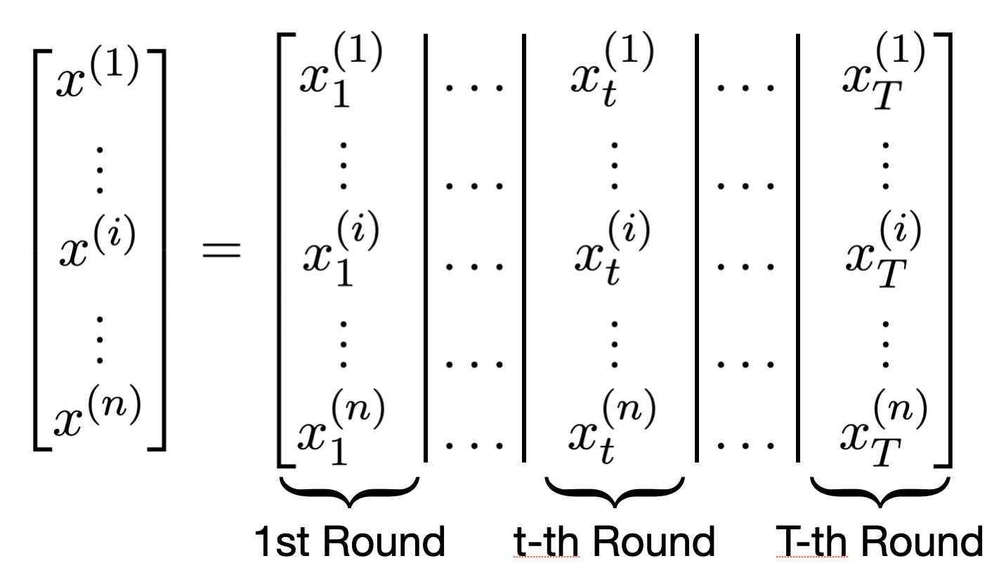
Figure 1: Each sample $x^{(i)}\in\mathbb{R}^{M}$ collected is divided into $T$ sub-vectors $x^{(i)}_{1},\cdots,x^{(i)}_{T}\in\mathbb{R}^{d}$ for $d=M/T$. Only the $x^{(i)}_{t}$’s are revealed in the $t$-th round.

Before we proceed, some remarks are in order. We start by noting that the task of online mean estimation without contamination (corresponding to the special case of $\epsilon=0$ in Definition 2) is not significantly more difficult than offline mean estimation. Indeed, in the noise-free setting, one can simply compute the sample mean and computing the $t$-th coordinate of the sample mean only requires the $t$-th coordinate of each sample. The contamination, however, dramatically complicates the situation. Specifically, all known robust mean estimators (even inefficient ones!) — including the Tukey median and its generalizations [Tuk75] or filtering based methods [DKK⁺16, DK21, DK23] — that achieve dimension-independent errors require looking at all coordinates of the sample at the same time. Prior to the current work, even the information-theoretic aspects of online robust mean estimation were not understood (i.e., what is the optimal error achievable when the sample size goes to infinity without computational considerations). Second, we remark that our formulation allows the mean estimation tasks across different time steps to be correlated. In particular, even though the sampling process between any two non-adversarial sensors are independent, the sampling results of one sensor (adversarial or not) at different time steps, namely the variables $x_{t}^{(i)}$ and $x_{t^{\prime}}^{(i)}$ for $t\neq t^{\prime}$, can be correlated.

In the rest of this section, we provide additional motivation for our robust online distribution learning model.

Federated Learning under Byzantine Failure

Federated learning is the practice of training an ML model in a distributed fashion on multiple decentralized worker devices containing local data; see [KMA⁺21] for an overview of the field. The typical framework is the following. At the $t$-th round, the central server broadcasts $w^{(t)}\in\mathbb{R}^{d}$ – the parameters of the central model – to all the worker devices. Then, each worker device makes updates to the central model received with their local data and sends back to the central server $w^{(t)}_{i}\in\mathbb{R}^{d}$ – the parameters of the updated local model. After receiving the responses from all local devices, the central server updates the central model by aggregating all the local models, producing a new estimate $w^{(t+1)}\leftarrow Aggregate(w_{i}^{(t)})$. A commonly used aggregation rule is called the FederatedAveraging algorithm: the central server simply computes the arithmetic mean of the updates [MMR⁺17]. One then iterates the training process until the central model reaches high accuracy on some validation set prepared in advance.

The distributed nature of the learning framework makes the task particularly vulnerable to Byzantine failures [LSP19] — a subset of malicious machines that behave adversarially in the computing network. As noted in the work of [PKH19], the FederatedAveraging algorithm, despite being one of the most commonly used aggregation protocols in practice, is especially vulnerable to Byzantine errors: even if only one worker device is controlled by the adversary, it can ruin the entire training process by giving wildly off local parameters in just one iteration.

The inherently unpredictable and possibly colluding adversarial behaviors of the Byzantine devices make them hard or even impossible to distinguish. This is especially true in an online or iterative learning procedure, including that of learning from streaming data or running distributed SGD, see, e.g., [CSX17], [BMGS17].

Proposed solutions usually involve performing robust estimation at each iteration independently [PKH19], [LXC⁺19]. This means that, though the adversary cannot corrupt the aggregation by too much at a single round, it can steadily create consistent errors in the training process. This scenario motivates our setup of considering robust mean estimation of multiple rounds in a holistic manner. In particular, our goal is to minimize the total error incurred in all rounds. As we will see later, it is indeed possible to design an efficient estimator such that the total errors only grow logarithmically with the number of rounds. This then opens up the hope of limiting the influence of Byzantine failures on online systems in the long run.

The above discussion illustrates two key principles for dealing with untrustworthy data. On the one hand, we can use outlier detection, to flag datapoints that might be erroneous. On the other hand, for sources that have been around for a while, we can additionally develop trust in a source based on the accuracy of previous predictions. In this paper, we will see how the interplay of these ideas can be used to maintain accurate estimates during ongoing data collection.

1.2 Our Results

We study the problem of high-dimensional online robust mean estimation in the setting of Definition 2. Our main results consist of (i) a computationally efficient robust online algorithm that achieves nearly optimal error rate (up to a factor of $\log T$, where $T$ is the number of rounds), and (ii) an inefficient robust online estimator that achieves the information-theoretically optimal error (within a constant factor).

Our first main result is a statistically and computationally efficient robust online algorithm that works generically for families of distributions commonly studied in the robust statistics literature (see Theorem 6 for a more general statement).

Theorem 1 (Efficient Online Robust Mean Estimation).

Let $\epsilon\leq\epsilon_{0}$ for a sufficiently small universal constant $\epsilon_{0}>0$. Suppose $X$ is an $M$-dimensional distribution with unknown mean vector $\mu^{\ast}\in\mathbb{R}^{M}$. There exists a computationally efficient algorithm which robustly estimates the mean of $X$ under $\epsilon$-corruption in the $T$-round online setting with failure probability $1/10$, sample complexity $n=\operatorname{poly}(M,1/\epsilon)$, and achieves the following error guarantees:

• If $X$ has unknown identity-bounded covariance (i.e., $\Sigma_{X}\preceq I$), then the algorithm achieves error $O(\sqrt{\epsilon}\log T)$.

• If $X$ is subgaussian with identity covariance, then the algorithm achieves error $O(\epsilon\sqrt{\log(1/\epsilon)}\log T)$.

Note that except for the $\log(T)$ factors above, the error bounds in Theorem 1 are optimal even for offline algorithms, i.e., algorithms allowed to observe the entire sample set $\mathcal{X}$ before having to make any predictions. Moreover, even though it is not explicitly specified in our theorem statements, we note that the sample complexity of our algorithm is near-optimal, matching that of the best known offline algorithm.

It is natural to ask whether this extra factor of $\log T$ is information-theoretically necessary for online robust mean estimation. In our second main contribution, we show that the $\log T$ factor can be removed for certain families of product distributions (albeit using an inefficient algorithm). See Theorem 11, Corollaries 14, 15 for details, and Theorem 12 for a more general statement.

Theorem 2 (Optimal Error for Product Distributions).

Let $\epsilon\leq\epsilon_{0}$ for a sufficiently small universal constant $\epsilon_{0}>0$. Fix two positive integers $M,T$ such that $T$ divides $M$. Suppose $X$ is an $M$-dimensional product distribution. Then there exists an (inefficient) algorithm which robustly estimates the mean of $X$ under $\epsilon$-corruption in the $T$-round online setting with failure probability $1/10$, sample complexity $n=2^{M}\cdot\operatorname{poly}(M,1/\epsilon)$, and achieves the following error guarantees:

• If $X$ is a Gaussian with identity covariance, then the algorithm achieves error $O(\epsilon)$.

• If $X$ has bounded $k$-th moments for $k\geq 4$, then the algorithm achieves error $O(\epsilon^{1-1/k})$.

• If $X$ is subgaussian with identity covariance, then the algorithm achieves error $O(\epsilon\sqrt{\log(1/\epsilon)})$.

Finally, we obtain a generalization of Theorem 2 that allows the independence of coordinates assumption to be slightly relaxed. In particular, we assume there is an unknown distribution $X_{t}$ chosen for the $t$-th round and the overall distribution $X$ is exactly the product of these $T$ unknown distributions. For this relaxed setting, we establish the following (see Theorem 16 for a more general statement).

Theorem 3 (Optimal Error for Round-wise Independent Distributions).

Let $\epsilon\leq\epsilon_{0}$ for a sufficiently small universal constant $\epsilon_{0}>0$. Let $X_{1},\cdots,X_{T}$ be $T$ unknown $d$-dimensional distributions. Suppose $X$ is the product distribution of $X_{1},\cdots,X_{T}$. Then there exists an (inefficient) algorithm which robustly estimates the mean of $X$ under $\epsilon$-corruption in the $T$-round online setting with failure probability $1/10$, sample complexity $n=2^{O(Td^{2})}\cdot\operatorname{poly}(1/\epsilon)$, and achieves the following error guarantees:

• If each $X_{i}$ has bounded $k$-th moments for $k\geq 4$, then the algorithm achieves error $O(\epsilon^{1-1/k})$.

• If each $X_{i}$ is subgaussian with identity covariance, then the algorithm achieves error $O(\epsilon\sqrt{\log(1/\epsilon)})$.

We remark that the aforementioned assumption on the distribution $X$ is a more general condition than the assumption that the coordinates of $X$ are mutually independent. In particular, this assumption holds as long as the estimation tasks for different rounds are independent of each other.

1.3 Overview of Techniques

The starting point of our efficient online algorithm is the weighted filtering algorithm for the offline robust mean estimation problem. The (offline) filtering algorithm works by assigning each sample a non-negative weight (initially set at $1/n$) that expresses our confidence that it is uncorrupted. Then, assuming that the uncorrupted samples satisfy a high probability stability assumption (see Definition 3), it applies a polynomial-time filtering technique in order to de-weight the worst outliers. In particular, assuming stability of the uncorrupted points, this filtering algorithm has two important properties. First, the total weight removed from uncorrupted points is at most the weight removed from corrupted ones (thus guaranteeing that at most $O(\epsilon)$ weight is removed overall). Second, after applying the filter, the weighted mean of the samples will be close to the true mean.

Our efficient algorithm essentially maintains an online version of this filter. This requires some new ideas that we explain in the proceeding discussion. In the online setting, we maintain a set of weights for each sample along with that sample’s currently revealed coordinates. In each round, we add the information about the newly revealed coordinates to each sample and re-apply our filter. We then return the weighted sample mean as our estimate for the mean for the newest block of coordinates. In particular, letting ${w}_{t}$ be the weight vectors at the end of the $t^{th}$ round and $\mu_{t}({w})$ be the average of the first $t$ blocks of data using weights ${w}$, our algorithm’s estimate for the $t^{th}$ block of coordinates is just the $t^{th}$ block of $\mu_{t}({w}_{t})$.

Now we know from the standard properties of the (offline) filter that $\|\mu_{t}({w}_{t})-\mu^{\ast}_{t}\|_{2}=O(\delta)$, where $\mu^{\ast}_{t}$ is the first $t$ blocks of the true mean and $\delta$ is the stability parameter. Unfortunately, this property alone does not suffice: it could be the case that $\mu_{t}({w}_{t})$ agrees exactly with $\mu_{t}^{\ast}$ in all but the $t^{th}$ block of coordinates, in which they differ by $\delta$. This would leave us with $\delta$ error on each block of coordinates, for a total error of $\delta\sqrt{T}$ finally. To avoid this possibility, we need a new and more subtle structural property of the filter algorithm. In particular, we show (see Lemma 3) that for any $t^{\prime}>t$ it holds $\sum_{j=1}^{t}\|\mu_{j}({w}_{t})-\mu_{j}({w}_{t^{\prime}})\|_{2}^{2}=O(\delta^{2}\|{w}_{t}-{w}_{t^{\prime}}\|_{1}/\epsilon).$ Since the total change in the weight vectors throughout the entire run of the algorithm is bounded by $O(\epsilon)$, this lemma allows us to show that once we assign values to a new block of coordinates, they cannot be changed too much by future reweightings. This property along with a careful recursive argument gives our final error bound of $O(\delta\log(T))$.

We now discuss the ideas behind our optimal error (inefficient) estimator. We start with the special case of binary product distributions. The high-level framework is the following. At the $t$-th round, the algorithm divides the samples into groups based on the revealed coordinates of the sample in the previous $t-1$ rounds (thus producing a total of $2^{t-1}$ groups). Equivalently, the samples within a group in some round will be divided into two child groups for the next round, based on the newly revealed coordinates. Given these groups, we then compute the mean of the $t^{th}$ coordinates of the samples in each group, and use as our final estimate the weighted median of these group means (weighted by group size). The robustness of this algorithm mainly follows from two observations. First, in each round, if the final estimation is $\eta$-far from the true mean, it must be the case that at least half of the group estimations (weighted by group size) are at least $\eta$-far from the true mean. Second, if the mean of a group is far from the true mean, then the adversarial samples must be divided unevenly among the two child groups in the next round. Consequently, as the algorithm accumulates more errors, the adversarial samples will become increasingly concentrated among a small fraction of groups. Since the final estimation is the median of all group estimations, it will become harder and harder to get the adversarial examples to influence the final mean. To formalize this intuition, we define a potential function, which is roughly the sum of the squares of the “adversarial densities” in each group weighted by its relative size (see Equation (8) for further details). In particular, we show (see Lemma 7) that if the algorithm produces an error of $\eta$ in the $t^{th}$ round, then the potential function must increase by $\Omega(\eta^{2})$ between rounds $t$ and $t+1$. Combined with the fact that the potential can never exceed $O(\epsilon^{2})$, this implies that this algorithm produces $\ell_{2}$-error of at most $O(\epsilon)$. A slight refinement of this argument shows that if each coordinate is known to have mean at most $\gamma$, then we can obtain error $O(\min(\epsilon,\sqrt{\gamma\epsilon}))$.

To obtain an online robust mean estimator for other families of product distributions, we use a reduction to the case of binary product distributions. In particular, if we define the indicator variables $Y(q)_{t}:=\mathbbm{1}\{X_{t}<q\}$, we note that for any $q$ that $Y(q)$ is a binary product distribution with mean $\mathbf{E}[Y(q)]_{t}={\bf{\rm Pr}}(X_{t}<q)$. Applying our binary product estimator to $Y(q)$, we can obtain relatively good estimates for the cumulative density functions of $X_{t}$ for all $t$. Using this, along with the formula $\mathbf{E}[X]=\int_{0}^{\infty}{\bf{\rm Pr}}(X<t)dt-\int_{0}^{\infty}{\bf{\rm Pr}}(X<-t)dt$, gives a suitable estimation of the mean of $X$ in an online fashion. For the details of this argument, see Section 4.

Finally, we discuss how our results can be further generalized to the case when the coordinates between rounds are independent — but the coordinates within a round are allowed to have arbitrary correlations. Once again, we would like to reduce to estimating the mean of binary product distributions by trying to estimate tail bounds. To see how this might work, we note that in the offline setting we can approximate the mean of $Z$ to error $O(\delta)$ if we can approximate the mean of $v\cdot Z$ to error $O(\delta)$ for every unit vector $v$ (or even for all $v$ in some finite cover of the sphere). This suggests the following idea. Denoting by $X_{t}$ the set of coordinates in the $t^{th}$ block, if we can estimate the mean of $v\cdot X_{t}$ for each unit vector $v$ and each $t$, this should provide the desired estimates for our mean. This idea seems promising as $[v\cdot X_{1},v\cdot X_{2},\ldots]$ is a product distribution. Unfortunately, a naive implementation of this will not work, as it might produce error on the order of $\sum_{t}\sup_{v}\mathrm{EstimationError}(v\cdot X_{t})^{2}$ — while our learner merely guarantees a bound on $\sup_{v}\sum_{t}\mathrm{EstimationError}(v\cdot X_{t})^{2}$. If different $v$’s produce different errors in different rounds, this could be much larger than we require. To fix this issue, we need a way of combining all of these estimators in order to correlate their errors.

To achieve this, we need to modify our binary product estimator. To estimate the means of $v\cdot X_{t}$ for a single $v$, we would break our samples into groups, based on whether or not $v\cdot x_{i}<s$ for each value of $i$, and then compute a mean in each group. For the new estimator, we instead break into groups based upon whether $v\cdot x_{i}<s$ for each $i$ and each $v$. This divides our sample set into many more groups in each round than the old algorithm did. However, if we are interested in estimating the mean of $v\cdot X_{t}$ for some particular vector $v$, we can think of this as first splitting into groups based on $v\cdot x_{i}<s$, and then breaking into smaller groups based on the other conditions. The thing to note here is that if our estimate of $\mathbf{E}[v\cdot X_{t}]$ had large error, then the first part of the subdivision would lead to a correspondingly large increase in our potential function, and then the further subdivisions based on other $v$’s would make it no smaller (despite not being independent anymore). This allows us to bound the errors in the stronger error model that we require. The details of this argument can be found in Appendix A.

1.4 Prior and Related Work

Here we record related literature that was not discussed earlier in the introduction.

(Offline) Algorithmic Robust Statistics

The goal of high-dimensional robust statistics is to efficiently obtain dimension-independent error guarantees for various statistical tasks in the presence of a constant fraction of adversarial outliers. Since the pioneering early work from the statistics community [Ans60, Tuk60, Hub64, Tuk75], there has been extensive work on designing robust estimators, see, e.g., [HRRS86, HR09] for early textbooks. Alas, the estimators proposed in the statistics community are computationally intractable to compute in high dimensions. The first algorithmic progress on high-dimensional robust statistics came in two independent works from the theoretical computer science community [DKK⁺16, LRV16]. Since the dissemination of these works, which mainly focused on high-dimensional robust mean and covariance estimation, the body of work in the field has grown rapidly. Prior work has obtained efficient algorithms with dimension-independent guarantees for various robust problems, including linear regression [KKM18, DKS19, BP21], stochastic optimization [PSBR20, DKK⁺19], and learning various mixture models [DKS18, KSS18, HL18, BDH⁺20, BK20, DHKK20, LM21, BDJ⁺22, DKK⁺22]. For a more detailed account, see the survey [DK21] and the recent book [DK23]. We emphasize that all these prior algorithms work in the offline setting, where the entire dataset is given in the input and the goal is to output a single estimate.

There are several natural ways to define “robust online distribution learning”, based on the underlying scenario to be modeled. Below we summarize prior work that falls into this general domain along with a comparison to our model.

Distributed Univariate “Online Robust Mean Estimation”

The recent work [YS22] studies the problem of robustly estimating the mean of a single univariate distribution when the data is distributed among $n$ clients and arrive in real time. At each time step, each agent receives either an i.i.d. sample from the distribution or a corrupted sample with some probability $\eta$. [YS22] gives a distributed algorithm such that the agents’ estimations reach consensus and converge to the true mean asymptotically. This contribution is largely orthogonal to our work. In particular, we point out two major differences with our setting. First, in our setting, the samples received at different time steps need not to be independent and identically distributed. In some sense, the setting of [YS22] is a special case of our setup where the unknown distribution is the product of $T$ identical distributions. Second, our corruption model is significantly stronger. In the setup of [YS22], each client has a fraction of adversarially corrupted samples while in our case there are a fraction of adversarial clients having only adversarially corrupted samples. We remark that our setup is closer to the Byzantine error model, typically assumed in the context of federated learning.

Robust Distributed Learning

A large number of works study distributed SGD in the presence of Byzantine Failures, see, e.g., [BMGS17], [SX19], [CSX17]. In that setting, a central server collects stochastic gradients from some worker devices. The gradients from most workers are assumed to be computed from i.i.d. samples and a small fraction of Byzantine devices may try to send arbitrary gradient updates to corrupt the training process. Typical approaches usually involve applying robust estimation techniques to aggregate the gradients received in each iteration. A closely related setting is that of robust federated learning; see, e.g., [PKH19], [LXC⁺19], [XCCL21]. Instead of aggregating the gradient, the central server now tries to directly aggregate the model parameters sent from the client device. Similarly, a small fraction of Byzantine devices may send arbitrary parameters to corrupt the central model parameters. The techniques applied in both settings are mostly iteration-independent, which means the accumulated estimation error always scales with the number of iterations. This is acceptable in these works, as the final goal is just to ensure that the final model output in the last round converges. We remark that this is different from our setting where the outputs in all rounds matter.

Robust Online Learning and Bandits

The works [TLL18, GKT19, BLKS21] study robust (linear) stochastic bandits, where the data is generated either from some i.i.d. distributions or adversarially corrupted data. In contrast to the typical contamination model assumed in robust statistics, the adversary can corrupt the reward of any action at any round, and the only restriction is that the difference between the actual reward and the corrupted reward needs to be bounded.

Another type of corruption model, investigated in [ABM19, MTCD21, KPK19, CKMY22], is the contaminated bandit model. Under this model, the rewards in most time steps are assumed to follow the underlying reward distributions and only a random small fraction of them may be replaced by arbitrary (unbounded) corrupted reward prepared by the adversary. This is closer to the corruption model considered in the robust statistics literature. We remark that our contamination model is still noticeably different. In particular, we observe many samples in each round and a constant fraction of the samples in each round are corrupted. Moreover, the distribution from which the inliers are generated can be different from round to round.

1.5 Discussion and Open Problems

This work introduces a natural model of online robust mean estimation capturing situations where a series of mean estimation tasks need to be completed sequentially, using data collected from the same set of sensors of which an $\epsilon$-fraction are malicious. We develop two types of algorithms for online robust estimation in this model: (i) an efficient algorithm that works for general distributions under the stability condition and achieves error which is optimal, up to a $\log T$ factor, where $T$ is the number of rounds; and (ii) an inefficient algorithm that works for more structured distributions (namely product distributions) and achieves the optimal error — with no dependence on $T$ whatsoever.

Our work raises a number of open questions, both technical and conceptual. First, one may wonder whether there is an algorithm that achieves the best of both worlds. Namely, it is statistically and computationally efficient and achieves error independent of $T$. This question is left open, even for identity covariance Gaussians. In fact, it is not even clear whether there exists an algorithm with polynomial sample complexity and error independent of $T$.

Question 4.

Are there statistically and/or computationally efficient algorithms for online robust mean estimation of identity covariance Gaussians, within error $\tilde{O}(\epsilon)$?

Our inefficient algorithms achieving optimal error leverage the assumption that the estimation tasks between rounds are independent. An interesting direction is to understand the role of “independence” in online robust mean estimation. Concretely, for general Gaussian distributions, it is unclear whether the optimal error achievable in the online setting is still the same as the offline problem.

Question 5.

What is the optimal error of online robust mean estimation of an unknown Gaussian distribution $N(\mu^{\ast},\Sigma^{\ast})$ (when the sample size goes to infinity)?

More generally, it would be interesting to go beyond mean estimation and explore the learnability of more general statistical tasks, including covariance estimation and linear regression, in our robust online learning model. The complexity of these tasks has by now been essentially characterized in the offline model. Understanding the possibilities and limitations in our robust online learning setting — both information-theoretic and computational — is a broad challenge for future work.

2 Preliminaries

Basic Notation

We use $\mathbbm{Z}^{+}$ to denote the set of positive integers and $\mathbb{R}^{+}$ to denote the set of positive reals. For $n\in\mathbbm{Z}^{+}$, we denote by $[n]$ the set of integers $\{1,\cdots,n\}$. For $d\in\mathbbm{Z}^{+}$, we use $\mathbb{R}^{d}$ to denote the set of $d$-dimensional real vectors. For $v\in\mathbb{R}^{d}$, we write $\left\|v\right\|_{2}$ to denote the $\ell_{2}$ norm of the vector $v$, i.e., $\left\|v\right\|_{2}=\sqrt{\sum_{i=1}^{d}v_{i}^{2}}$. If $M$ is a symmetric matrix, we write $\left\|M\right\|_{2}$ to denote the largest eigenvalue (in absolute value) of $M$. The asymptotic notation $\tilde{O}$ (resp. $\tilde{\Omega}$) suppresses logarithmic factors in its argument, i.e., $\tilde{O}(f(n))=O(f(n)\log^{c}f(n))$ and $\tilde{\Omega}(f(n))=\Omega(f(n)/\log^{c}f(n))$, where $c>0$ is a universal constant. Given $x_{1},\cdots,x_{k}\in\mathbb{R}^{+}$, we write $\operatorname{poly}(x_{1},\cdots,x_{k})$ to denote a sufficiently large constant degree polynomial in $\Pi_{i=1}^{k}x_{i}$. For a univariate random variable $X$ and $q\in\mathbb{R}$, we use $\mathbf{E}[X]$ for its expectation and $\mathbbm{1}\{X>q\}$ for the indicator of the event $X>q$. Given a set of samples $\{x^{(1)},\cdots,x^{(n)}\}\in\mathbb{R}^{M}$, we often write $x^{(1:n)}$ to represent the set. Let $x\in\mathbb{R}^{T\cdot d}$ be the concatenation of $T$ sub-vectors $x_{1},\cdots x_{T}\in\mathbb{R}^{d}$. We will write $\bar{x}_{t}$ to represent the partition vector that is the concatenation of the vectors $x_{1},\cdots,x_{t}$. Whenever we write $\bar{x}_{t}$, the partition of $x$ into the sub-vectors $x_{1},\cdots,x_{T}$ should be clear from the context.

Stability Condition

Our efficient algorithm works for any sample set satisfying the well-studied stability property (see [DK21]).

Definition 3 (($\epsilon,\delta$)-stability).

For $\epsilon\in(0,1/2)$ and $\delta\geq\epsilon$, a finite set $S\subset\mathbb{R}^{d}$ is $(\epsilon,\delta)$-stable with respect to a vector $\mu\in\mathbb{R}^{d}$ if for every unit vector $v\in\mathbb{R}^{d}$ and every subset $S^{\prime}\subseteq S$, where $|S^{\prime}|\geq(1-\epsilon)|S|$, the following conditions are satisfied:

1. $\left|\frac{1}{|S^{\prime}|}{\sum_{x\in S^{\prime}}v^{T}\cdot\left(x-\mu\right)}\right|\leq\delta.$

2. $\left|\frac{1}{|S^{\prime}|}\sum_{x\in S^{\prime}}\big{(}v^{T}\cdot(x-\mu)\big{)}^{2}-1\right|\leq\delta^{2}/\epsilon.$

A stable set $S$ satisfies that any sufficiently large subsets of $S$ can produce accurate enough first and second moment estimations, captured by the parameters $\epsilon$ and $\delta$.

This stability condition (or variants thereof) has been proven critical for robust mean estimation algorithms even in the offline setting. In particular, essentially all known efficient algorithms for learning the mean of a distribution from $\epsilon$-corrupted samples to error $\delta$ require some condition on the uncorrupted samples at least as strong as $(\epsilon,\delta)$-stability. As such, it will be important for us to know that our sample set satisfies this condition. This problem has been extensively studied in the literature (see, e.g., [DK21]). For example, we have the following results:

1. If $S$ is a set of i.i.d. samples from a distribution of identity-bounded covariance $\Sigma\preceq{I}$ and $|S|=\tilde{\Omega}(d/\epsilon)$, then with high probability $S$ is $(\epsilon,O(\sqrt{\epsilon}))$-stable.

2. If $S$ is a set of i.i.d. samples from a subgaussian distribution with identity covariance $\Sigma={I}$ and $|S|=\tilde{\Omega}(d/\epsilon^{2})$, then with high probability $S$ is $(\epsilon,O(\epsilon\sqrt{\log(1/\epsilon)}))$-stable.

We here remark a simple property of stability that is particularly useful for the online setup. Let $\{x^{(1)},\cdots,x^{(n)}\}\subset\mathbb{R}^{T\cdot d}$ be a set of samples satisfying the $(\epsilon,\delta)$-stability condition with respect to some vector $\mu\in\mathbb{R}^{T\cdot d}$. Consider the partition of coordinates into $T$ parts such that $x^{(i)}$ is the concatenation of $x^{(i)}_{1},\cdots,x^{(i)}_{T}\in\mathbb{R}^{d}$ for $i\in[n]$ and $\mu$ is the concatenation of $\mu_{1},\cdots,\mu_{T}\in\mathbb{R}^{d}$. Then, for all $t\in[T]$, the set $\{\bar{x}^{(1)}_{t},\cdots,\bar{x}^{(n)}_{t}\}\subset\mathbb{R}^{d\cdot t}$ is also $(\epsilon,\delta)$-stable with respect to vector $\bar{\mu}_{t}\in\mathbb{R}^{d\cdot t}$.

In the rest of the paper, we assume that the initial uncorrupted sample set $\mathcal{C}$ is $(\epsilon,\delta)$-stable. We use $\mathcal{X}$ to denote the $\epsilon$-corrupted version of $\mathcal{C}$ under the strong contamination model. and we use $\mathcal{H}$ to denote the set of clean samples in $\mathcal{X}$, i.e. $\mathcal{H}=\mathcal{C}\cap\mathcal{X}$. Consequently, $\mathcal{X}\setminus\mathcal{H}$ represents the corrupted samples.

3 Efficient Online Robust Mean Estimation

In this section, we describe our computationally efficient algorithm for online robust mean estimation, thereby establishing Theorem 1. Before stating our approach, we describe a natural attempt and discuss why it fails.

We start by observing that the naive approach of applying the offline weighted filter to the data $\{x^{(1)}_{t},\cdots,x^{(n)}_{t}\}$ revealed in the $t$-th round independently does not suffice. Such a naive algorithm will incur error $\epsilon^{\prime}$ (achievable by the optimal offline filter algorithm) in each round, leading to a final $\ell_{2}$ error of $\sqrt{T\cdot\left(\epsilon^{\prime}\right)^{2}}=\epsilon^{\prime}\sqrt{T}$. As hinted at the end of Section 1.1, a key idea in online robust estimation is the interplay between filtering outliers and establishing “trust” over the data providers. Hence, a natural idea is to let the filtering algorithm in the $(t+1)$-th round to “inherit” the information about how likely each sample $x^{(i)}$ is an outlier from the filtering result in the $t$-th round.

Suppose we are using the weighted filtering algorithm which produces a set of weights $w^{(i)}_{t}$ for each sample $i\in[n]$ at the end of the $t$-th round. We can then initialize the weights for the filtering algorithm in the $(t+1)$-th round as exactly $w^{(i)}_{t}$. Unfortunately, the idea to simply maintain an online version of the weights achieves little improvement in the worst case. Consider the case where the unknown distribution $X$ is the product of $T$ isotropic Gaussians $X_{1},\cdots,X_{T}$. Then the adversary can contaminate the set of samples $\mathcal{C}$ to make them look like i.i.d. samples from another isotropic Gaussian distribution $X^{\prime}_{t}$ for each round $t\in[T]$, such that $\left\|\mathbf{E}[X^{\prime}_{t}]-\mathbf{E}[X_{t}]\right\|_{2}=c\cdot\epsilon$ for some constant $c$ [DK21]. Then the filtering algorithm should not downweight any sample, since the revealed coordinates in each round $t$ of contaminated samples are statistically indistinguishable from i.i.d. samples from $X^{\prime}_{t}$. As a result, the algorithm’s error still grows with $\sqrt{T}$, but the weight remains unchanged throughout the process.

We address this issue by considering the aggregation of all historical records. At the $t$-th round, we will concatenate the vectors $x_{1}^{(i)},\cdots,x_{t}^{(i)}$ together into $\bar{x}_{t}^{(i)}\in\mathbb{R}^{t\cdot d}$ and perform filtering on the dataset $\bar{x}_{t}^{(1:n)}$. In particular, after initializing the weight $w^{(1:n)}_{0}$ as $1/n$, our algorithm repeats the following two main procedures: (a) concatenate the coordinates of each sample revealed so far, denoted by $\bar{x}^{(i)}_{t}=(x^{(i)}_{1},\cdots,x^{(i)}_{t})$ for $i\in[n]$; (b) apply filters to iteratively decrease the weights $w^{(1:n)}_{t-1}$ inherited from the last round until the set $\bar{x}^{(1:n)}_{t}$ under the new weights $w^{(1:n)}_{t}$ satisfies the appropriate second moment condition. Our proposed efficient online algorithm is presented in pseudocode as Algorithm 1 below. Intuitively, via operation (a), Algorithm 1 ensures that the estimation made in the $t$-th round properly utilizes all historical information; and through operation (b) that the weights adjust to reflect the “likelihood” of a sample being an outlier as the algorithm collects more information.

Recall that in the offline setting (loading the entire data set $\mathcal{X}$ and computing the estimation once), the information-theoretically optimal error guarantee under the $(\epsilon,\delta)$-stability condition is $\Theta(\delta)$. Somewhat surprisingly, the above technique in the online setting yields an error that has only an extra $\log T$ factor.

Theorem 6.

Suppose that $\mathcal{C}$ is $(\epsilon,\delta)$-stable with respect to $\mu^{*}$ and $X$ is an $\epsilon$-corrupted version of $\mathcal{C}$. Then, for $\epsilon$ at most a sufficiently small positive constant, there exists some constant $\kappa$ such that Algorithm 1, when $\lambda=\kappa\delta^{2}/\epsilon$, outputs a sequence of estimates satisfying

$$\left\|\mu-\mu^{*}\right\|_{2}=O(\delta\log T)\;.$$

In the following, we present the proof of Theorem 6. With the stability assumption of clean data in mind, we list a few properties of the offline weighted filter algorithm that will be used in the analysis. Given a proper selection of filtering threshold $\lambda$ dependent upon the stability parameters, in every round the filter always removes more weighted mass from the adversarial samples compared to that from honest/clean samples. As the set of vectors in $\mathcal{C}$ truncated to the coordinates revealed so far remains stable and Algorithm 1 iteratively applies the filter, Algorithm 1 inherits this property. Therefore, given a limited budget $\epsilon$ of the adversary, Algorithm 1 will finally terminate to find a proper weight set satisfying the desired second moment bound.

We formally state this as the following lemma.

Algorithm 1 Online Filter

1:  Input: The number of samples $n$, Byzantine fraction $\epsilon$, round number $T$, sample coordinates $x^{(1:n)}_{t}$ revealed at the $t^{th}$ round for $t=1,2,\cdots,T$, filter threshold $\lambda$, and initialized weight $w^{(i)}_{0}=1/n$, for $i=1,2,\cdots,n$.

2:  for $t=1,2,\cdots,T$ do

3:     Initialize ${w}_{t}\leftarrow{w}_{t-1}$ and update $\bar{{x}}^{(i)}_{t}=(x^{(i)}_{1},...,x^{(i)}_{t})$.

4:     Compute $\Sigma\leftarrow\text{WCov}({w}_{t},\bar{{x}}^{(1:n)}_{t})$.

5:     while $\|\Sigma\|_{2}>1+\lambda$ do

6:        Compute the top eigenvector $v$ of $\Sigma$.

7:        Compute empirical weighted mean $\mu({w}_{t})\leftarrow\sum_{i=1}^{n}w^{(i)}_{t}\bar{{x}}^{(i)}_{t}.$

8:        for $i=1,2,\cdots,n$ do

9:           Compute $\rho^{(i)}\leftarrow\langle v,{x}^{(i)}-\mu({w}_{t})\rangle^{2}$.

10:        end for

11:        Sort $\rho^{(1:n)}$ into a decreasing order denoted as $\rho^{\pi(1)}\geq\rho^{\pi(2)}\geq\cdots\geq\rho^{\pi(n)}$, and let $\beta$ be the smallest number such that $\sum_{i=1}^{\beta}\rho^{\pi(i)}>2\epsilon.$

12:        Apply WFilter to update weights for $\{\pi(1),\cdots,\pi(\beta)\}$ as $\{w^{\pi(1)}_{t},\cdots,w^{\pi(\beta)}_{t}\}\leftarrow\text{WFilter}(\rho^{\pi(1:\beta)},w^{\pi(1:\beta)}_{t})$; while the remaining weights keep the same, i.e., $w^{\pi(i)}_{t}=w^{\pi(i)}_{t}$ for $i>\beta$.

13:        Update $\Sigma\leftarrow\text{WCov}({w}_{t},\bar{{x}}^{(1:n)}_{t})$

14:     end while

15:     Output: $\mu_{t}=\sum_{i=1}^{n}w^{(i)}_{t}x^{(i)}_{t}$.

16:  end for

Subroutine 1: Weighted Filter (WFilter)

1:  Input: scores $\rho^{\pi(1:\beta)}$, weights $w^{\pi(1:\beta)}$.

2:  for $i=1,2,...,\beta$ do

3:     $w^{\pi(i)}\leftarrow(1-\frac{\rho^{\pi(i)}}{\max_{j}\rho^{\pi(j)}})w^{\pi(i)}.$

4:  end for

5:  Output: $w^{\pi(1:\beta)}$.

Subroutine2: Weighted Covariance (WCov)

1:  Input: weight ${w}=w^{(1:n)}$ and samples $\bar{x}^{(1:n)}$.

2:  Compute $\mu({w})\leftarrow\sum_{i=1}^{n}\frac{w^{(i)}}{\|{w}\|_{1}}\bar{x}^{(i)}.$

3:  Compute weighted covariance estimation $\Sigma\leftarrow\sum_{i=1}^{n}\frac{w^{(i)}}{\|{w}\|_{1}}(\bar{x}^{(i)}-\mu({w}))(\bar{x}^{(i)}-\mu({w}))^{T}.$

4:  Output: $\Sigma$.

Lemma 1 (Proposition 2.13 of [DK21]).

When $\mathcal{C}$ is $(\epsilon,\delta)$-stable, $\mathcal{X}$ is an $\epsilon$ corrupted version of $\mathcal{C}$, and $\epsilon<\epsilon_{0}$ for some sufficiently small $\epsilon_{0}$, there exists some constant $\kappa$ such that in Algorithm 1 when $\lambda\geq\kappa\delta^{2}/\epsilon$, for any $t\in[T]$, $\sum_{i\in\mathcal{H}}w^{(i)}_{t-1}-\sum_{i\in\mathcal{H}}w^{(i)}_{t}\leq\sum_{i\in\mathcal{X}\setminus\mathcal{H}}w^{(i)}_{t-1}-\sum_{i\in\mathcal{X}\setminus\mathcal{H}}w^{(i)}_{t}.$

It is also worth noting that at the end of the filter step in any round, the empirical covariance matrix $\Sigma=\text{WCov}({w}_{t},\bar{{x}}^{(1:n)}_{t})$ satisfies $\|\Sigma\|_{2}\leq 1+\lambda$. In fact, by stability of $\mathcal{C}$, the weighted covariance of just the points in $\mathcal{H}$ must be at least $1-O(\delta^{2}/\epsilon)$ in every direction, and so if $\lambda$ is an appropriate multiple of $\delta^{2}/\epsilon$, we will have that $\|\Sigma\|_{2}\leq 1+\lambda$. This second moment bound then allows us to control the error in our estimate of the mean. In particular, we have:

Lemma 2 (Lemma 2.4 of [DK21]).

If $\mathcal{X}=\{x^{(1)},...,x^{(n)}\}$ is an $\epsilon$-corrupted version of an $(\epsilon,\delta)$-stable set $\mathcal{C}$ with respect to $\mu$ and $\epsilon<\epsilon_{0}$ for some sufficiently small $\epsilon_{0}$, then for any selection of weights $w^{(1:n)}$ such that $\sum_{i=1}^{n}|1/n-w^{(i)}|\leq 2\epsilon$,

$$\|\mu({w})-\mu\|_{2}\leq O(\delta+\sqrt{\epsilon\cdot{\max\{(\|\Sigma({w})\|_{2}-1),0\}}}),$$

where the empirical mean is denoted by $\mu({w})=\sum_{i=1}^{n}\frac{w^{(i)}}{\|{w}\|_{1}}x^{(i)}$, and the empirical covariance $\Sigma({w})=\sum_{i=1}^{n}\frac{w^{(i)}}{\|{w}\|_{1}}(x^{(i)}-\mu({w}))(x^{(i)}-\mu({w}))^{T}$.

Lemma 2 states that the error in the empirical estimate of the mean is controlled by the empirical covariance. In particular, after filtering we can guarantee that $\|\Sigma({w})\|_{2}-1\leq\lambda$, and consequently guarantee a mean estimation error of $O(\delta+\sqrt{\epsilon\lambda})=O(\delta)$. For an offline robust mean estimation algorithm, the above properties would be enough to show the error guarantees of the algorithm. To analyze the behavior of the algorithm in the online setting, we need a more subtle property of the filtering algorithm: the difference in the estimations of $\mu_{t}^{*}$ using weights from two different rounds is proportional to the difference in the weights. The formal statement is given below.

Lemma 3.

Given the assumptions of Theorem 6, for $1\leq t<t^{\prime}\leq T$, let $\mu({w}_{t},\bar{{x}}^{(1:n)}_{t})=\sum_{i=1}^{n}\frac{w^{(i)}_{t}\bar{{x}}^{(i)}_{t}}{\|{w}_{t}\|_{1}}$ and $\mu({w}_{t^{\prime}},\bar{{x}}^{(1:n)}_{t})=\sum_{i=1}^{n}\frac{w^{(i)}_{t^{\prime}}\bar{{x}}^{(i)}_{t}}{\|{w}_{t^{\prime}}\|_{1}}$. Then, when we apply Algorithm 1, it holds that

$$\left\|\mu({w}_{t},\bar{{x}}^{(1:n)}_{t})-\mu({w}_{t^{\prime}},\bar{{x}}^{(1:n)}_{t})\right\|_{2}^{2}\leq O(1)\cdot\frac{\delta^{2}}{\epsilon}\cdot\left\|{w}_{t}-{w}_{t^{\prime}}\right\|_{1}.$$

Proof.

Let ${y}_{t}={w}_{t}/\|{w}_{t}\|_{1}$ and ${y}_{t^{\prime}}={w}_{t^{\prime}}/\|{w}_{t^{\prime}}\|_{1}$ be the normalized weight outputted at the round $t$ and $t^{\prime}$, respectively, and $\eta=\|{y}_{t}-{y}_{t^{\prime}}\|_{1}$. We consider the following decomposition ${y}_{t}=(1-\eta){y}_{t^{\prime}}+\eta{e},$ where ${e}$ is a non-zero weight vector with $\|{e}\|_{1}=1$. Notice that ${y}_{t}$, ${y}_{t^{\prime}}$, and ${e}$ can be thought as distributions over our sample vectors ${\bar{x}}^{(i)}_{t}$. Essentially, the distribution under ${y}_{t}$ is a mixture of the distributions under ${y}_{t^{\prime}}$, and ${e}$ respectively. This implies that

$$\textbf{Cov}({y}_{t})=(1-\eta)\cdot\textbf{Cov}({y}_{t^{\prime}})+\eta\cdot\textbf{Cov}({e})+\eta(1-\eta)\cdot\Big{(}\mu({y}_{t^{\prime}})-\mu(e)\Big{)}\Big{(}\mu({y}_{t^{\prime}})-\mu({e})\Big{)}^{T},$$

where $\textbf{Cov}(\cdot)$ and $\mu(\cdot)$ denote the covariance and mean over $\bar{x}^{(i)}_{t}$ respectively under the argument inside. Since both $\|\textbf{Cov}({y}_{t})-I\|_{2}$ and $\|\textbf{Cov}({y}_{t^{\prime}})-I\|_{2}$ are $O(\delta^{2}/\epsilon)$ and since $\textbf{Cov}({e})\succeq 0$, we have that $\|\mu({y}_{t^{\prime}})-\mu({e})\|_{2}^{2}=O(\delta^{2}/(\eta\epsilon)).$ Combining this with the fact that

$$\mu({y}_{t})-\mu({y}_{t^{\prime}})=(1-\eta)\cdot\mu({y}_{t^{\prime}})+\eta\cdot\mu({e})-\mu({y}_{t^{\prime}})=-\eta\cdot\Big{(}\mu({y}_{t^{\prime}})-\mu({e})\Big{)}$$

then yields $\left\|\mu({y}_{t})-\mu({y}_{t^{\prime}})\right\|_{2}^{2}\leq O\left(\eta\cdot\delta^{2}/\epsilon\right).$ Finally, notice that, by definition, $\mu(y_{t})$ is exactly $\mu(w_{t},\bar{x}^{(1:n)}_{t})$(and similarly for $\mu(y_{t}^{\prime})$ and $\mu(w_{t}^{\prime},\bar{x}^{(1:n)}_{t})$), and $\eta=O(\left\|w_{t}-w_{t}^{\prime}\right\|_{1})$. Our lemma follows. ∎

The error guarantee of Algorithm 1 then largely follows from the following two observations: (i) after the last round, if we were to use the weights ${w}_{T}$ in hindsight to estimate the means in each round, the error will be optimal since the algorithm is essentially the same as the one used in the offline setting; (ii) $\mu({w}_{t},{\bar{x}}^{(1:n)}_{t})$, the estimation outputted at the $t^{th}$ round, will not differ much from $\mu({w}_{t^{\prime}},{\bar{x}}^{(1:n)}_{t})$, the estimation if we were to use the weights $w_{t^{\prime}}$ from some future round $t^{\prime}>t$. We note that (i) simply follows from the standard guarantees of the filtering algorithm while (ii) follows from Lemma 3 and Lemma 1. Formally, we show the cumulative $L^{2}$ difference between the mean estimations produced across $T$ time slots and that from the last round can be bounded by $O(\log^{2}T)$ through a careful recursive argument.

Lemma 4.

$\sum_{t=1}^{T}\|\mu({w}_{t},{{x}}^{(1:n)}_{t})-\mu({w}_{T},{{x}}^{(1:n)}_{t})\|_{2}^{2}\leq O\left(\log^{2}T\cdot\delta^{2}\right)$.

Proof.

We begin by reviewing a few key facts about our algorithm.

Firstly, we note that, since the algorithm only decreases weights it will be the case that $w^{(i)}_{1}\geq w^{(i)}_{2}\geq\ldots\geq w^{(i)}_{T}$, for any $i$, and in particular $\|{w}_{t}-{w}_{t^{\prime}}\|_{1}=\|{w}_{t}\|_{1}-\|{w}_{t^{\prime}}\|_{1}$ for any $1\leq t\leq t^{\prime}\leq T$. It also follows that $\|{w}_{1}\|_{1}\geq\|{w}_{2}\|_{1}\geq\ldots\|{w}_{T}\|_{1}$.

Secondly, we note that by Lemma 1 our algorithm removes more mass from bad elements than good. Since the initial mass of the bad elements is only at most $\epsilon$, this implies $\|{w}_{1}\|_{1}-\|{w}_{T}\|_{1}=O(\epsilon).$

Finally, we note by Lemma 3 that for all $t^{\prime}>t$ and sufficiently large $C_{0}$

$$\sum_{l=1}^{t}\left\|\mu({w}_{t},{{x}}^{(1:n)}_{l})-\mu({w}_{t^{\prime}},{{x}}^{(1:n)}_{l})\right\|_{2}^{2}=\left\|\mu({w}_{t},\bar{{x}}^{(1:n)}_{t})-\mu({w}_{t^{\prime}},\bar{{x}}^{(1:n)}_{t})\right\|_{2}^{2}\leq C_{0}\cdot\frac{\delta^{2}}{\epsilon}\cdot(\|{w}_{t}\|_{1}-\|{w}_{t^{\prime}}\|_{1}).$$ (1)

Our goal will now be to prove that for any two rounds $a<b$ and any sufficiently large $\sqrt{C}>3\sqrt{C_{0}}$ that:

$$\sum_{t=a}^{b}\|\mu({w}_{t},{{x}}^{(1:n)}_{t})-\mu({w}_{b},{{x}}^{(1:n)}_{t})\|_{2}^{2}\leq C\left(\log^{2}(1+b-a)\cdot(\|{w}_{a}\|_{1}-\|{w}_{b}\|_{1})\cdot\frac{\delta^{2}}{\epsilon}\right).$$ (2)

In particular, we will prove this by strong induction on $b-a$.

The base case here is when $b=a+1$, in which case, Equation (2) follows immediately from Equation (1). For the inductive step, consider $c=\lfloor(a+b)/2\rfloor$. Then, we note that

$$\sum_{t=a}^{b}\|\mu({w}_{t},{{x}}^{(1:n)}_{t})-\mu({w}_{b},{{x}}^{(1:n)}_{t})\|_{2}^{2}=\sum_{t=a}^{c}\|\mu({w}_{t},{{x}}^{(1:n)}_{t})-\mu({w}_{b},{{x}}^{(1:n)}_{t})\|_{2}^{2}+\sum_{t=c+1}^{b}\|\mu({w}_{t},{{x}}^{(1:n)}_{t})-\mu({w}_{b},{{x}}^{(1:n)}_{t})\|_{2}^{2}.$$

By the inductive hypothesis, we bound the second term by

$$C\left(\log^{2}(1+b-c)\cdot(\|{w}_{c}\|_{1}-\|{w}_{b}\|_{1})\cdot\frac{\delta^{2}}{\epsilon}\right)\leq C\left((\log(1+b-a)-1/2)^{2}\cdot(\|{w}_{c}\|_{1}-\|{w}_{b}\|_{1})\cdot\frac{\delta^{2}}{\epsilon}\right).$$

By triangle’s inequality, the first term is at most

$$\sum_{t=a}^{c}\left(\|\mu({w}_{t},{{x}}^{(1:n)}_{t})-\mu({w}_{c},{{x}}^{(1:n)}_{t})\|_{2}+\|\mu({w}_{c},{{x}}^{(1:n)}_{t})-\mu({w}_{b},{{x}}^{(1:n)}_{t})\|_{2}\right)^{2}.$$ (3)

For convenience, we will denote

$$\alpha =\sum_{t=a}^{c}\|\mu({w}_{t},{{x}}^{(1:n)}_{t})-\mu({w}_{c},{{x}}^{(1:n)}_{t})\|_{2}^{2}$$

$$\beta =\sum_{t=a}^{c}\|\mu({w}_{c},{{x}}^{(1:n)}_{t})-\mu({w}_{b},{{x}}^{(1:n)}_{t})\|_{2}^{2}.$$

Then, it is easy to see that Equation (3) is at most $\alpha+\beta+2\sqrt{\alpha\beta}$.

Our inductive hypothesis tells us that

$$\alpha\leq C\left(\log^{2}(1+c-a)\cdot(\|{w}_{a}\|_{1}-\|{w}_{c}\|_{1})\cdot\frac{\delta^{2}}{\epsilon}\right)\leq C\left((\log(1+b-a)-1/2)^{2}\cdot(\|{w}_{a}\|_{1}-\|{w}_{c}\|_{1})\cdot\frac{\delta^{2}}{\epsilon}\right),$$

and Equation (1) tells us that

$$\beta\leq C_{0}\cdot\frac{\delta^{2}}{\epsilon}\cdot(\|{w}_{a}\|_{1}-\|{w}_{c}\|_{1}).$$

Thus, combining the above, we find that $\sum_{t=a}^{b}\|\mu({w}_{t},{{x}}^{(1:n)}_{t})-\mu({w}_{b},{{x}}^{(1:n)}_{t})\|_{2}^{2}$, as desired, is at most

$$C\left((\log(1+b-a)-1/2)^{2}\cdot(\|{w}_{c}\|_{1}-\|{w}_{b}\|_{1})\cdot\frac{\delta^{2}}{\epsilon}\right)$$

$$+C\left((\log(1+b-a)-1/2)^{2}\cdot(\|{w}_{a}\|_{1}-\|{w}_{c}\|_{1})\cdot\frac{\delta^{2}}{\epsilon}\right)+\beta+2\sqrt{\alpha\beta}$$

$$\leq(\delta^{2}/\epsilon)\cdot\left(\|{w}_{a}\|_{1}-\|{w}_{b}\|_{1}\right)\left(C(\log^{2}(1+b-a)-\log(1+b-a))+C_{0}+2\sqrt{CC_{0}\log^{2}(1+b-a)}\right)$$

$$\leq(\delta^{2}/\epsilon)\cdot\left(\|{w}_{a}\|_{1}-\|{w}_{b}\|_{1}\right)\left(C\log^{2}(1+b-a)-C\log(1+b-a)+3\log(1+b-a)\sqrt{CC_{0}}\right)$$

$$\leq C\left(\log^{2}(1+b-a)\cdot\left(\|{w}_{a}\|_{1}-\|{w}_{b}\|_{1}\right)\cdot\delta^{2}/\epsilon\right).$$

Note that the last line above depends on the selection that $\sqrt{C}\geq 3\sqrt{C_{0}}$. This completes our proof of Equation (2), and plugging in $a=1$ and $b=T$ completes the proof of this lemma. ∎

Finally, with all the above preparation, we can prove the statement in Theorem 6. First, from Lemma 1, the weights do not increase and once the second moment criterion is not satisfied, more mass will be removed from the adversary side. Therefore, given the bounded $\epsilon$ budget for the adversary, Algorithm 3 will finally terminate to find ${w}_{T}$ such that the empirical covariance $\|\Sigma({w}_{T})-{I}\|\leq\lambda$, for some sufficiently large $\lambda\geq\kappa\delta^{2}/\epsilon$. Moreover, it must terminate in at most $\epsilon\cdot n$ filter iterations since the weights of at least $1$ point becomes $0$ after each filter iteration. Then, by Lemma 2, it holds

$$\sum_{t=1}^{T}\|\mu({w}_{T},{x}^{(1:n)}_{t})-\mu^{*}_{t}\|^{2}=\|\mu({w}_{T},{\bar{x}}^{(1:n)}_{T})-{\mu}^{*}\|^{2}\leq O(\delta^{2}).$$ (4)

Combining Lemma 4 with Equation (4), we then have

$$\sum_{t=1}^{T}\|\mu({w}_{t},{x}^{(1:n)}_{t})-\mu^{*}_{t}\|^{2} =\sum_{t=1}^{T}\|\mu({w}_{t},{x}^{(1:n)}_{t})-\mu({w}_{T},{x}^{(1:n)}_{t})+\big{(}\mu({w}_{T},{x}^{(1:n)}_{t})-\mu^{*}_{t}\big{)}\|^{2}$$

$$\leq 2\big{(}\sum_{t=1}^{T}\|\mu({w}_{t},{x}^{(1:n)}_{t})-\mu({w}_{T},{x}^{(1:n)}_{t})\|^{2}+\|\mu({w}_{T},{x}^{(1:n)}_{t})-\mu^{*}_{t}\|^{2}\big{)}$$

$$=O(\delta^{2}+{\delta^{2}}\log^{2}T).$$

Thus, Theorem 6 follows.

Remark 7.

Throughout the analysis, we relied on only two properties of the filter algorithm: (i) the algorithm at each step filters more corrupted sample points than uncorrupted ones, and (ii) the filter in each round terminates when the rest of samples truncated to the coordinates revealed so far have bounded covariance. We note that the extra $\log T$ factor in our analysis of the filter algorithm in Theorem 6 is nearly tight if one does not leverage any additional property of the filtering algorithm. In particular, consider a special case of the theorem where the clean set $C$ is a set that has its covariance bounded by some constant multiple of $I$. Then, let $X^{(1)},\cdots X^{(T)}$ be sets of samples such that $X^{(t)}$ represents the samples kept by the filter algorithm until the $t$-th round (assume the filter algorithm always sets the weight of a sample to be either $0$ or $1$). We show that if $X^{(1)},\cdots X^{(T)}$ are sets satisfying only properties (i) and (ii), the output of the algorithm can incur an $\ell_{2}$ error as large as $\Omega(\epsilon\log T)$. For more details of this, see Appendix B.

4 Optimal Error for Product Distributions

In this section, we establish Theorem 2. We start with the special case of binary product distributions (Section 4.1) and develop on optimal error (inefficient) algorithm in this setting. We then show that our upper bound for binary products can be used as a subroutine to perform optimal error online robust mean estimation for more general families of product distributions, including identity covariance Gaussians (Section 4.2) and product distributions whose coordinates can even come from nonparametric families, as long as they satisfy mild concentration properties (Section 4.3).

4.1 Binary Product Distributions

In this section, we present an algorithm which robustly estimates the mean of binary product distributions in the online setting and achieves the optimal accuracy. As we will see in proceeding sections, the algorithm can also be used as a building block to obtain online mean estimations for many other important families of distributions.

For this purpose, it is useful to consider binary product distributions whose coordinate-wise means are uniformly bounded by some constant $\gamma\in(0,1)$. We will call such distributions “$\gamma$-bounded” binary product distributions.

Definition 4 ($\gamma$-Bounded Binary Product Distribution).

Let $X$ be a distribution on the boolean hypercube $\{0,1\}^{M}$. We say $X$ is a binary product distribution if its coordinates are mutually independent. Additionally, it is $\gamma$-bounded if each coordinate $X_{i}$ satisfies $\mathbf{E}[X_{i}]\leq\gamma$ for $i\in[M]$.

We briefly discuss robust mean estimation of such distributions in the offline model. When $\epsilon$-fraction of the samples are generated adversarially, it is possible to approximate the mean within $\ell_{2}$ distance $O(\epsilon)$ for any binary product distribution (not necessarily $\gamma$-bounded). Importantly, this is information-theoretically optimal, in the sense that no algorithm can distinguish between two binary product distributions whose means differ by $\Omega(\epsilon)$ given a dataset of any size such that $\epsilon$-fraction of the data points are corrupted.

However, when we have the extra condition that the mean of the unknown distribution is coordinate-wise bounded by $\gamma$, for some $\gamma<\epsilon$, it turns out we can take advantage of the condition to improve our estimation accuracy. In particular, it can be shown that any two $\gamma$-bounded binary product distributions within total variation distance $\epsilon$ have their mean differ by at most $\sqrt{\epsilon\gamma}$ in $\ell_{2}$-distance. Hence, it is possible to estimate the means of $\gamma$-bounded binary product distributions up to accuracy $O(\min(\epsilon,\sqrt{\epsilon\gamma}))$ in the offline model. Without too much extra effort, it is easy to see the accuracy is also information-theoretically optimal. As the main theorem of the section, we show this optimal accuracy is still achievable in the online setting.

In the following section, we restrict our attention to the setting when only one coordinate is revealed in each round, i.e., $d=1$ and $M=T$. This is a strictly harder setting, as we can always simulate the process of revealing the coordinates one at a time even when $d>1$. Hence, in the rest of this section, we will always have $d=1$ and the unknown distribution $X$ is always a $T$-dimensional distribution.

Theorem 8.

Let $\epsilon,\gamma,\tau\in(0,1)$. Suppose $X$ is a $T$-dimensional $\gamma$-bounded binary product distribution. For sufficiently small $\epsilon$, there exists an algorithm Binary-Product-Estimation which robustly estimates the mean of $X$ under $\epsilon$ corruption in the online setting with error $O(\min(\epsilon,\sqrt{\gamma\epsilon}))$, failure probability $\tau$, and sample complexity

$$n\geq 2^{T}\cdot\operatorname{poly}(T,1/\epsilon,1/\gamma)\cdot\log(1/\tau)\;.$$

Algorithm 2 Binary-Product-Estimation

1:  Input: The number of samples $n$, Byzantine fraction $\epsilon$, round number $T$, sample coordinates $\{x^{(1)}_{t}\,\cdots x^{(n)}_{t}\}$ revealed at $t$-th iteration for $t=1,2,\cdots,T$, bound parameter $\gamma$.

2:  Initialize the group $S_{0}^{(1)}=[n]$.

3:  for $t=1,2,...,T$ do

4:     In the $t$-th round, $x_{t}^{(1)},\cdots,x_{t}^{(n)}$ are revealed.

5:     for $i=0,\cdots,2^{t-1}-1$ do

6:        Compute the group estimation $\mu_{t}^{(i)}\stackrel{{\scriptstyle{\mathrm{\footnotesize def}}}}{{=}}\min\left(\gamma,\frac{1}{|S_{i}^{(t)}|}\sum_{j\in S_{i}^{(t)}}x^{(j)}_{t}\right)$.

7:        Split to create the child groups.

$$S_{2\cdot i}^{(t+1)}=\{j\in S_{i}^{(t)}\text{ such that }x_{t}^{(j)}=0\}\,,S_{2\cdot i+1}^{(t+1)}=\{j\in S_{i}^{(t)}\text{ such that }x_{t}^{(j)}=1\}.$$

8:     end for

9:     Set $\mu_{t}$ to be the weighted median over $\mu_{t}^{(i)}$ where the weights are given by $\left|S_{i}^{(t)}\right|$.

10:     Output: $\mu_{t}$.

11:  end for

Preliminary Simplification

We will manually add noise to the samples in the following manner. At the $t$-th round, for each sample $i\in[n]$, we change $x_{t}^{(i)}$ to $1$ with probability $\gamma/4$, to $0$ with probability $1/2-\gamma/4$ and leaves it unchanged otherwise. Then, the samples after the preprocessing can be viewed as i.i.d. samples drawn from another binary product distribution $X^{\prime}$ satisfying that $\mathbf{E}[X^{\prime}_{t}]=\mathbf{E}[X_{t}]/2+\gamma/4$. It is easy to see that then we have $\mathbf{E}[X^{\prime}_{t}]\in[\gamma/4,3\cdot\gamma/4]$. Furthermore, if our algorithm outputs $\mu^{\prime}$ such that $\left\|\mu^{\prime}-\mathbf{E}[X^{\prime}]\right\|_{2}\leq\xi$. Then, we can easily compute $\mu$ where $\mu_{t}\stackrel{{\scriptstyle{\mathrm{\footnotesize def}}}}{{=}}2\cdot\mu^{\prime}_{t}-\gamma/2$ such that $\left\|\mu-\mathbf{E}[X]\right\|_{2}\leq O(\xi)$. Hence, with this preprocessing step, we will assume without loss of generality that the unknown distribution $X$ satisfies $\mathbf{E}[X_{t}]\in[\gamma/4,3\cdot\gamma/4]$.

Main Algorithm

At the beginning of the $t$-th round, the algorithm divides the samples into at most $2^{t-1}$ groups based on the $0,1$ patterns of the past observations. In particular, the group $S_{i}^{(t)}$ consists of all samples of index $j$ satisfying $\bar{x}^{(j)}_{t-1}=\text{Binary}(i)$. Within each group $i\in[2^{t-1}]$, we compute the group estimation $\mu^{(i)}_{t}\stackrel{{\scriptstyle{\mathrm{\footnotesize def}}}}{{=}}\min\left(\gamma,\frac{1}{|S_{i}^{(t)}|}\sum_{j\in S_{i}^{(t)}}x^{(j)}_{t}\right)$, which is essentially the empirical mean within the group capped by $\gamma$ - the known upper bound for the true mean $\mu_{t}^{*}$. Then, we will compute the weighted median $\mu_{t}$, i.e. the median of the distribution $U$ such that $\Pr\left[U=\mu_{t}^{(i)}\right]\propto\left|S_{i}^{(t)}\right|$.

At a high level, our algorithm relies on the following simple but useful fact. Let $\mathcal{C}$ be the set of clean samples and $\mathcal{C}_{i}^{(t)}\stackrel{{\scriptstyle{\mathrm{\footnotesize def}}}}{{=}}S_{i}^{(t)}\cap\mathcal{C}$ denote the set of clean samples within the group $S_{i}^{(t)}$. Then, the empirical mean of $S_{i}^{(t)}$ can only be far from $\mathcal{C}_{i}^{(t)}$ if there are far more adversarial samples (in $S_{i}^{(t)}$) having one label than the other. In other words, the adversarial samples needs to be allocated unevenly among the child group branched off from $S_{i}^{(t)}$ for the sample mean of $S_{i}^{(t)}$ to be severely corrupted. As a result, if we were going to compute the sample means of the two child groups in the $(t+1)$-th round, one of them will be “cleaner” as it is less affected by the adversaries. In long term, if the adversaries keep corrupting the sample mean of each group, the adversarial samples will get increasingly concentrated within a small fraction of groups, leaving the sample means of the vast majority of groups relatively uncorrupted. Though we cannot necessarily identify the cleaner groups, we can nonetheless take the median of the sample means of all groups, and the estimator will get increasingly more reliable in the future rounds as it incurs more errors in the past rounds.

We now outline the proof which formalizes the above high-level intuition. First, we show that the empirical mean of the clean samples within each group are well-concentrated around the true mean (Lemma 5). Condition on that, we then formally spell out our observation of the relationship between the errors of the estimation of a group and the distribution of adversarial samples among its child groups and show its correctness. (Lemma 6). Finally, we define a potential function which intuitively measures how “concentrated” the adversarial samples are and couple it with the error guarantees of the algorithm (Lemma 7).

For the mean estimation task to be possible even without the interference of the adversaries, we need the mean of the clean samples is at least well-concentrated around the true mean. Since our algorithm breaks the samples into many groups, we require the empirical mean of the clean samples within each group to be sufficiently accurate. We show this is true with high probability.

Lemma 5.

Let $\hat{\mu}^{(i)}_{t}$ be the empirical mean of the group $S_{i}^{(t)}$ computed from only the clean samples. In particular, let $\mathcal{C}$ denote the set of un-corrupted samples. We define $\hat{\mu}^{(i)}_{t}\stackrel{{\scriptstyle{\mathrm{\footnotesize def}}}}{{=}}\frac{1}{\left|\mathcal{C}\cap S_{i}^{(t)}\right|}\sum_{i\in\mathcal{C}\cap S_{i}^{(t)}}x_{t}^{(i)}.$ Assume that $n\geq 2^{T}\cdot\operatorname{poly}(T,1/\epsilon,1/\gamma)\cdot\log(1/\tau)$. With probability at least $1-\tau$, for all $t$ and any group satisfying that $|S_{i}^{(t)}\cap\mathcal{C}|\geq n\cdot\epsilon/2^{t-1}$ , it holds $\left|\hat{\mu}^{(i)}_{t}-\mu_{t}^{*}\right|\leq\min\left(\epsilon,\gamma\right)/T$.

Proof.

The guarantee will be violated if there is any group such that (i) $|S_{i}^{(t)}\cap\mathcal{C}|\geq n\cdot\epsilon/2^{t-1}$ and (ii) $\left|\hat{\mu}^{(i)}_{t}-\mu_{t}^{*}\right|\geq\min\left(\epsilon,\gamma\right)/T$. Fix a group $S_{i}^{(t)}$, we argue the probability such that (i) and (ii) happens at the same time is small and conclude our proof with the union bound. Since the probability $\Pr[A\cap B]$ for two events is always smaller than $\Pr[A|B]$, it suffices for us to argue that $\left|\hat{\mu}^{(i)}_{t}-\mu_{t}^{*}\right|\geq\min\left(\epsilon,\gamma\right)/T$ happens with small probability condition on $|S_{i}^{(t)}\cap\mathcal{C}|\geq n\cdot\epsilon/2^{t-1}$. Notice that under the condition, $\hat{\mu}^{(i)}_{t}$ is exactly the average of $n\cdot\epsilon/2^{t-1}$ i.i.d. copies of a binary variable with mean $\mu_{t}^{*}$. Then, by Chernoff bound, we easily have $\left|\hat{\mu}^{(i)}_{t}-\mu_{t}^{*}\right|\leq\min\left(\epsilon,\gamma\right)/T$ with probability at least $1-\tau/(10T\cdot 2^{T})$ since $n\cdot\epsilon/2^{t-1}\geq\operatorname{poly}(T,1/\epsilon,1/\gamma)\cdot\log(1/\tau)$. Then, by union bound, this holds for all groups with probability at least $1-\tau$ since there are at most $T\cdot 2^{T}$ many groups. ∎

The algorithm is deterministic once the samples are drawn. We will condition on the guarantee in Lemma 5 being true in the proceeding analysis and show that the algorithm always succeeds. A quantity crucial to the analysis of the algorithm is the Adversarial Density of each group.

Definition 5.

At the $t$-th iteration, we define $\epsilon_{i}^{(t)}$, the adversarial density of a group $S_{i}^{(t)}$, to be the fraction of adversarial samples within $S_{i}^{(t)}$.

Consider the two child groups, $S_{L(i)}^{(t+1)}$ and $S_{R(i)}^{(t+1)}$ , branched from $S_{i}^{(t)}$ in the next round. In particular, we have

$$S_{L(i)}^{(t+1)}=\left\{j\in S_{i}^{(t)}\text{ such that }x_{t}^{(j)}=1\right\}\,,S_{R(i)}^{(t+1)}=\left\{j\in S_{i}^{(t)}\text{ such that }x_{t}^{(j)}=0\right\}.$$

Assume that $S_{i}^{(t)}$ has enough clean samples ( $\left|S_{i}^{(t)}\cap\mathcal{C}\right|\geq\operatorname{poly}(T,1/\epsilon,1/\gamma)\cdot\log(1/\tau)$ ) such that the empirical mean $\hat{\mu}_{t}^{(i)}$ computed from the clean samples are close to $\mu_{t}^{*}$. Then, if the group estimation $\mu_{t}^{(i)}$ from the group $S_{i}^{(t)}$ is still far from the true mean $\mu_{t}^{*}$, it must be the case that the adversarial samples are distributed unevenly among the groups $S_{L(i)}^{(t+1)},S_{R(i)}^{(t+1)}$. We formalize the intuition in the argument below.

Lemma 6.

Let $S_{i}^{(t)}$ be a group satisfying that (i) $\left|S_{i}^{(t)}\cap\mathcal{C}\right|\geq n\cdot\epsilon/2^{t-1}$ (ii) $\epsilon_{i}^{(t)}\leq 10\epsilon$. Let $S_{L(i)}^{(t+1)},S_{R(i)}^{(t+1)}$ be the two child groups branched from $S_{i}^{(t)}$. Assume the group estimation $\mu_{t}^{(i)}$ is off by $\eta\stackrel{{\scriptstyle{\mathrm{\footnotesize def}}}}{{=}}\left|\mu_{t}^{(i)}-\mu_{t}^{*}\right|\geq 2\cdot\min\left(\epsilon,\gamma\right)/T$. Then, if $\left|S_{L(i)}^{(t+1)}\right|/\left|S_{i}^{(t)}\right|\leq 5\gamma$, it holds

$$\left|\epsilon_{L(i)}^{(t+1)}-\epsilon_{R(i)}^{(t+1)}\right|\geq\Omega(\eta)\cdot\left|S_{i}^{(t)}\right|/\left|S_{L(i)}^{t+1}\right|.$$

Otherwise, we have

$$\left|\epsilon_{L(i)}^{(t+1)}-\epsilon_{R(i)}^{(t+1)}\right|\geq\Omega(1).$$

Proof.

Notice that $\epsilon_{i}^{(t)}$ can be viewed as the following convex combination of $\epsilon_{L(i)}^{(t+1)}$ and $\epsilon_{R(i)}^{(t+1)}$.

$$\frac{\left|S_{L(i)}^{(t+1)}\right|}{\left|S_{i}^{(t)}\right|}\cdot\epsilon_{L(i)}^{(t+1)}+\frac{\left|S_{R(i)}^{(t+1)}\right|}{\left|S_{i}^{(t)}\right|}\cdot\epsilon_{R(i)}^{(t+1)}=\epsilon_{i}^{(t)}.$$

Hence, it must be that $\left|\epsilon_{L(i)}^{(t+1)}-\epsilon_{R(i)}^{(t+1)}\right|=\left|\epsilon_{L(i)}^{(t+1)}-\epsilon_{i}^{(t)}\right|+\left|\epsilon_{R(i)}^{(t+1)}-\epsilon_{i}^{(t)}\right|.$ It hence suffices for us to lower bound $\left|\epsilon_{L(i)}^{(t+1)}-\epsilon_{i}^{(t)}\right|$. Since we condition on the guarantee in Lemma 5 being true, the first condition $\left|S_{i}^{(t)}\cap\mathcal{C}\right|\geq n\cdot\epsilon/2^{t-1}$ ensures that the empirical mean computed from the clean samples is relatively accurate.

$$\left|\hat{\mu}_{t}^{(i)}-\mu_{t}^{*}\right|\leq\min\left(\epsilon,\gamma\right)/T.$$ (5)

Case I: $\left|S_{L(i)}^{(t+1)}\right|/\left|S_{i}^{(t)}\right|>5\gamma$. In this case, we claim that the group $S_{L(i)}^{(t+1)}$ is mostly made up of adversarial samples. By Equation (5), we have that there are at most

$$\hat{\mu}_{t}^{(i)}\cdot(1-\epsilon_{i}^{(t)})\cdot\left|S_{i}^{(t)}\right|\leq\left(\mu_{t}^{*}+\gamma/T\right)\cdot(1-\epsilon_{i}^{(t)})\cdot\left|S_{i}^{(t)}\right|\leq 2\gamma\cdot\left|S_{i}^{(t)}\right|$$

many clean samples. On the other hand, since we have $\left|S_{L(i)}^{(t+1)}\right|/\left|S_{i}^{(t)}\right|>5\gamma$ in this case, it holds there are at least $3\gamma\cdot\left|S_{i}^{(t)}\right|$ many adversarial samples. Hence, the adversarial density for $S_{L(i)}^{(t+1)}$ is at least $3/5$. Therefore, we have $\left|\epsilon_{L(i)}^{(t+1)}-\epsilon_{i}^{(t)}\right|\geq\Omega(1)$.
Case II: $\left|S_{L(i)}^{(t+1)}\right|/\left|S_{i}^{(t)}\right|<5\gamma$. Let $a_{L(i)}^{(t+1)}$ be the number of adversarial samples within $S_{L(i)}^{(t+1)}$ and $\tilde{\mu}_{t}^{(i)}$ as the uncapped empirical mean of the group, i.e. $\tilde{\mu}_{t}^{(i)}=\frac{\left|S_{L(i)}^{(t+1)}\right|}{\left|S_{i}^{(t)}\right|}$. We can always write the number of samples in $S_{L(i)}^{(t+1)}$ as the sum of clean samples and adversarial samples.

$$\left|S_{L(i)}^{(t+1)}\right|=a_{L(i)}^{(t+1)}+\hat{\mu}_{i}^{(t)}(1-\epsilon_{i}^{(t)})\cdot\left|S_{i}^{(t+1)}\right|.$$ (6)

Rearranging Equation (6) then gives

$$\left|a_{L(i)}^{(t+1)}-\hat{\mu}_{i}^{(t)}\cdot\epsilon_{i}^{(t)}\cdot\left|S_{i}^{(t+1)}\right|\right|=\left|\tilde{\mu}_{t}^{(i)}-\hat{\mu}_{i}^{(t)}\right|\cdot\left|S_{i}^{(t+1)}\right|.$$

We assume that the group estimation is off by $\eta\geq 2\cdot\min\left(\epsilon,\gamma\right)/T$. The uncapped group mean is off by at least that much since “capping” the group mean always draws it closer to the true mean $\mu_{t}^{*}$. This gives us

$$\left|\tilde{\mu}_{t}^{(i)}-\mu_{t}^{*}\right|\geq\left|\mu_{t}^{(i)}-\mu_{t}^{*}\right|=\eta\geq 2\cdot\min(\epsilon,\gamma)/T.$$

On the other hand, the empirical mean of the clean samples are accurate enough such that $\left|\hat{\mu}_{t}^{(i)}-\mu_{t}^{*}\right|\leq\epsilon/T$. By triangle’s inequality we then have $\left|\tilde{\mu}_{t}^{(i)}-\hat{\mu}_{i}^{(t)}\right|\geq\eta/2\,,$ which further implies that

$$\left|a_{L(i)}^{(t+1)}-\hat{\mu}_{i}^{(t)}\cdot\epsilon_{i}^{(t)}\cdot\left|S_{i}^{(t+1)}\right|\right|\geq\eta/2\cdot\left|S_{i}^{(t+1)}\right|.$$ (7)

Notice that $\epsilon_{L(i)}^{t+1}$ and $a_{L(i)}^{t+1}$ have the following relationship

$$\epsilon_{L(i)}^{(t+1)}=\frac{a_{L(i)}^{(t+1)}}{a_{L(i)}^{t+1}+\hat{\mu}_{t}^{(i)}\cdot\left(1-\epsilon_{i}^{(t)}\right)\cdot\left|S_{i}^{(t)}\right|}.$$

Thus, we can rewrite $\left|\epsilon_{L(i)}^{(t+1)}-\epsilon_{i}^{(t)}\right|$ as

$$\left|\epsilon_{L(i)}^{(t+1)}-\epsilon_{i}^{(t)}\right|=\left|\frac{a_{L(i)}^{t+1}-\epsilon_{i}^{(t)}\cdot\left(a_{L(i)}^{t+1}+\hat{\mu}_{t}^{(i)}\cdot\left(1-\epsilon_{i}^{(t)}\right)\cdot\left|S_{i}^{(t)}\right|\right)}{a_{L(i)}^{t+1}+\hat{\mu}_{t}^{(i)}\cdot\left(1-\epsilon_{i}^{(t)}\right)\cdot\left|S_{i}^{(t)}\right|}\right|=\frac{\left|a_{L(i)}^{t+1}-\epsilon_{i}^{(t)}\hat{\mu}_{t}^{(i)}\left|S_{i}^{(t)}\right|\right|\cdot\left(1-\epsilon_{i}^{(t)}\right)}{a_{L(i)}^{t+1}+\hat{\mu}_{t}^{(i)}\cdot\left(1-\epsilon_{i}^{(t)}\right)\cdot\left|S_{i}^{(t)}\right|}.$$

Notice that the denominator is simply $\left|S_{L(i)}^{(t+1)}\right|$. Hence, combining this with Equation (7) then gives

$$\left|\epsilon_{L(i)}^{(t+1)}-\epsilon_{i}^{(t)}\right|\geq\Omega(\eta)\cdot\frac{\left|S_{i}^{(t)}\right|}{\left|S_{L(i)}^{t+1}\right|}.$$

∎

As the algorithm keeps accumulating errors, the adversarial samples will become increasingly concentrated in a small fraction of groups. Since the final output of the algorithm is given by the weighted median of the estimations from all groups, it therefore gets harder for the adversary to corrupt the estimation as the algorithm accumulates more errors. This then allows us to design a potential function based on the adversarial density to bound the total error incurred.

Potential Function

To bound the total error of the estimation, we consider the following potential function,

$$\Phi(t)\stackrel{{\scriptstyle{\mathrm{\footnotesize def}}}}{{=}}\frac{1}{N}\sum_{i=1}^{2^{t-1}}g_{\gamma}\left(\epsilon_{i}^{(t)}\right)\cdot\left|S_{i}^{(t)}\right|\,,$$ (8)

where $g_{\gamma}:[0,1]\mapsto\mathbb{R}^{+}$ is the piecewise function

$$g_{\gamma}(x)=\begin{cases}x^{2}&\text{if }x<10\cdot\epsilon/\gamma\,,\\ 20\frac{\epsilon}{\gamma}\cdot x-100\left(\frac{\epsilon}{\gamma}\right)^{2}&\text{otherwise.}\end{cases}$$

Here, we briefly discuss the reasons for using such a piecewise function $g_{\gamma}$ to construct the potential function. In essence, $g_{\gamma}$ is designed to have the following properties.

Claim 9.

$g_{\gamma}$ is (i) convex within the entire domain $[0,1]$ (ii) $2$-strongly convex within the interval $[0,10\epsilon/\gamma]$ (iii) upper bounded by $O\left(\min\left(\epsilon/\gamma,1\right)\right)$.

Proof.

One can verify that for all $x,y$ where $g_{\gamma}^{\prime}(x),g_{\gamma}^{\prime}(y)$ is well-defined, we have $g_{\gamma}^{\prime}(x)<g_{\gamma}^{\prime}(y)$ as long as $x<y$. In particular, for all $x<10\epsilon/\gamma$, $g_{\gamma}^{\prime}(x)=2x$, which is indeed a monotonically increasing function. For all $x10\epsilon/\gamma$, we have $g_{\gamma}^{\prime}(x)=20\epsilon/\gamma$, which is constant. Moreover, $2\cdot 10\epsilon/\gamma=20\epsilon/\gamma$. Hence, for any $x<10\epsilon/\gamma$ and $y\geq 10\epsilon/\gamma$, we always have $g^{\prime}_{\gamma}(x)\leq g_{\gamma}^{\prime}(y)$. Besides, at the kink $c=10\epsilon/\gamma$ , we have $\lim_{x\rightarrow c^{+}}g_{\gamma}(x)=\lim_{x\rightarrow c^{-}}g_{\gamma}(x)$, showing that $g_{\gamma}$ is a continuous function. The convexity of $g_{\gamma}$ then follows. Within the interval $[0,10\epsilon/\gamma]$, $g_{\gamma}$ is simply the quadratic function $x^{2}$. Hence, it is $2$-strongly convex. Finally, we derive the upper bound for $g_{\gamma}$ through a case analysis. Since $g_{\gamma}$ is monotonically increasing, $\max_{x}g_{\gamma}(x)$ is always attained at $g(1)$. When $10\epsilon/\gamma>1$. $g_{\gamma}(x)=x^{2}$ over the entire domain $[0,1]$. We then have $\max_{x}g_{\gamma}(x)=g_{\gamma}(1)=1$. When $10\epsilon/\gamma<1$, we have $g_{\gamma}(1)\leq 20\epsilon/\gamma$. Both quantities are of order $O\left(\min(\epsilon/\gamma,1)\right)$ in their regimes, therefore giving the desired upper bound. ∎

When a group $S_{i}^{(t)}$ splits into two child groups $S_{L(i)}^{(t+1)}$, $S_{R(i)}^{(t+1)}$, we always have that

$$\epsilon_{i}^{(t)}=\frac{\left|S_{L(i)}^{(t+1)}\right|}{\left|S_{i}^{(t)}\right|}\cdot\epsilon_{L(i)}^{(t+1)}+\frac{\left|S_{R(i)}^{(t+1)}\right|}{\left|S_{i}^{(t)}\right|}\cdot\epsilon_{R(i)}^{(t+1)}.$$

Therefore, the convexity of $g_{\gamma}$ then ensures that the total contribution from the child groups is at least the contribution from the parent group. , making $\Phi$ a valid non-decreasing “potential”. Besides, $g_{\gamma}(x)$ is locally strongly convex. This ensures the contribution to the potential will increase substantially if the adversarial densities between the two child groups differ by a lot (given that their adversarial densities are still within the strongly convex region of $g_{\gamma}$ ). Lastly, the upper bound on $g_{\gamma}$ allows us to derive tight upper bound for the potential function, which is essential in obtaining the optimal error bound for the algorithm. We give the upper bound on $\Phi$ below.

Claim 10.

$\Phi(t)\leq O(1)\cdot\min\left(\epsilon,\epsilon^{2}/\gamma\right)$ for all $t\in[T]$.

Proof.

Notice that we always have the equality

$$\sum_{i}\frac{\left|S_{i}^{(t)}\right|}{n}\cdot\epsilon_{i}^{(t)}=\epsilon.$$

Since $g_{\gamma}$ is a convex function, it is not hard to see that the potential function is maximized when we have $\epsilon$ fraction of groups that are made entirely of adversarial samples. This then gives that

$$\Phi(t)\leq\epsilon\cdot g_{\gamma}(1)\leq O(1)\cdot\min\left(\epsilon,\epsilon^{2}/\gamma\right).$$

∎

We next show how we can couple the increment of the potential function and the estimation error incurred. At a high level, if our algorithm outputs $\mu_{t}$ such that it incurs error $\eta\stackrel{{\scriptstyle{\mathrm{\footnotesize def}}}}{{=}}\left|\mu_{t}-\mu_{t}^{*}\right|$, more than half of the group estimations $\mu_{t}^{(i)}$ must also be off by at least $\eta$ since $\mu_{t}$ is obtained by computing the median over $\mu_{t}^{(i)}$. As illustrated in Lemma 6, given that such an erroneous group also satisfies some other technical conditions, the adversarial density for one of its child group must be substantially higher than the other. Then, strong-convexity of $g_{\gamma}$ will ensure the contributions to the potential from the child groups must be significantly higher than that from the parent group. One slight issue of the above argument is that the adversarial densities of these erroneous groups (and their child groups) may be well above the threshold $10\epsilon/\gamma$. For such a group, even if the split of the adversarial samples is vastly uneven between the two child groups, their overall contribution to the potential remains the same since both of them are in the linear regime for $g_{\gamma}$. Fortunately, there cannot be too many groups with high adversarial densities, and it suffices for us to look at only the increments gained from groups with relatively low adversarial densities.

Lemma 7.

$\Phi(t+1)-\Phi(t)\geq\Omega(1/\gamma)\cdot\left(\mu_{t}-\mu_{t}^{*}\right)^{2}$ if $\left|\mu_{t}-\mu_{t}^{*}\right|\geq 2\cdot\min\left(\epsilon,\gamma\right)/T$.

Proof.

We first introduce some notations. Let $S_{L(i)}^{(t+1)},S_{R(i)}^{(t+1)}$ be the two child groups branched off from the parent group $S_{i}^{(t)}$. Let $\epsilon_{L(i)}^{(t+1)}\,,\epsilon_{R(i)}^{(t+1)}$ be their corresponding adversarial densities, and $\hat{\mu}_{t}^{(i)}$ be the empirical mean computed from the clean samples from the parent group $S_{i}^{(t)}$. For each group $S_{i}^{(t)}$, we define its increment as

$$\Delta\left(S_{i}^{(t)}\right)\stackrel{{\scriptstyle{\mathrm{\footnotesize def}}}}{{=}}\left(\frac{|S_{L(i)}^{(t+1)}|}{n}\right)\cdot g_{\gamma}\left(\epsilon_{L(i)}^{(t+1)}\right)+\left(\frac{|S_{R(i)}^{(t+1)}|}{n}\right)\cdot g_{\gamma}\left(\epsilon_{R(i)}^{(t+1)}\right)-\left(\frac{\left|S_{i}^{(t)}\right|}{n}\right)\cdot g\left(\epsilon_{i}^{(t)}\right).$$ (9)

Consider the groups satisfying the following conditions (i) $\epsilon_{i}^{(t)}\leq 5\epsilon$ (ii) the estimation $\mu_{t}^{(i)}$ is off from $\mu_{t}^{*}$ by at least $\left|\mu_{t}^{(i)}-\mu_{t}^{*}\right|\geq\eta\stackrel{{\scriptstyle{\mathrm{\footnotesize def}}}}{{=}}\left|\mu_{t}-\mu_{t}^{*}\right|$, which is by our assumption at least $2\cdot\min(\epsilon,\gamma)/T$, and (iii) the number of clean samples is at least $\left|S_{i}^{(t)}\cap\mathcal{C}\right|\geq n\cdot\epsilon/2^{t-1}$. Notice that the total weight of groups satisfying condition (i) is at least $1-1/5$, the total weight of groups satisfying condition (ii) is at least $1/2$. For condition (iii), we claim the total weight of groups satisfying that is at least $1-2\cdot\epsilon$. Since there are only $\epsilon$ fraction of adversarial samples, we have $\sum_{i}\left|S_{i}^{(t)}\cap\mathcal{C}\right|=n\cdot(1-\epsilon)$. Let $\mathcal{H}$ be the set of groups which satisfy the condition. Then, we have

$$\sum_{i\in\mathcal{H}}\left|S_{i}^{(t)}\cap\mathcal{C}\right|\geq n\cdot(1-\epsilon)-\sum_{i\not\in\mathcal{H}}\left|S_{i}^{(t)}\cap\mathcal{C}\right|\geq n\cdot(1-\epsilon)-n\cdot\epsilon\,,$$

where in the second inequality we use the fact that $\left|S_{i}^{(t)}\cap\mathcal{C}\right|\leq n\cdot\epsilon/2^{t-1}$ for $i\not\in\mathcal{H}$ and there are at most $2^{t-1}$ many groups. Then, our claim easily follows from the fact that $\left|S_{i}^{(t)}\right|\geq\left|S_{i}^{(t)}\cap\mathcal{C}\right|$. Denote the set of groups satisfying all three conditions as $G$. By union bound, it is not hard to see that the fraction of groups satisfying the above three conditions is at least

$$\frac{1}{n}\sum_{i\in G}\left|S_{i}^{(t)}\right|\geq 1/5.$$ (10)

We will show that, for each group $i\in G$, the contribution to the potential function from the two child groups branched off from $i$ in the next round is significantly higher than the contribution from the $i$-th group at the current round. In particular, for all $i\in G$, we claim its increment is at least

$$\Delta\left(S_{i}^{(t)}\right)\geq\frac{\left|S_{i}^{(t)}\right|}{n}\cdot\Omega(\eta^{2}/\gamma).$$ (11)

For any other groups $i\not\in G$, we instead show the contributions to the potential are non-decreasing. In particular, for all $i\not\in G$, we claim

$$\Delta\left(S_{i}^{(t)}\right)\geq 0.$$ (12)

Again, $\epsilon_{i}^{(t)}$ can be viewed as the following convex combination of $\epsilon_{L(i)}^{(t+1)},\epsilon_{R(i)}^{(t+1)}$.

$$\frac{S_{L(i)}^{(t+1)}}{S_{i}^{(t)}}\cdot\epsilon_{L(i)}^{(t+1)}+\frac{S_{R(i)}^{(t+1)}}{S_{i}^{(t)}}\cdot\epsilon_{R(i)}^{(t+1)}=\epsilon_{i}^{(t)}\,,$$

and the increment can be rewritten as

$$\Delta\left(S_{i}^{(t)}\right)=\frac{\left|S_{i}^{(t)}\right|}{n}\cdot\left(\frac{|S_{L(i)}^{(t+1)}|}{\left|S_{i}^{(t)}\right|}\cdot g_{\gamma}(\epsilon_{L(i)}^{(t+1)})+\frac{|S_{R(i)}^{(t+1)}|}{\left|S_{i}^{(t)}\right|}\cdot g_{\gamma}(\epsilon_{R(i)}^{(t+1)})-g_{\gamma}(\epsilon_{i}^{(t)})\right)\;.$$ (13)

Hence, Equation (12) immediately follows from the convexity of $g_{\gamma}$.

Next, we proceed to show Equation (11). By 9, $g_{\gamma}$ is $2$-strongly convex within the interval $[0,10\epsilon/\gamma]$. We will show that $\epsilon_{L(i)}^{(t+1)},\epsilon_{R(i)}^{(t+1)}$ are both within the region where $g_{\gamma}$ is strongly convex. By our choice of the group $i$, we have $\epsilon_{i}^{(t)}\leq 5\epsilon$, and $\left|S_{i}^{(t)}\cap\mathcal{C}\right|\geq n\cdot\epsilon/2^{t-1}$. Then, by Lemma 5, it holds that $\left|\hat{\mu}_{t}^{(i)}-\mu^{*}_{t}\right|\leq\gamma/T$. Then, we can upper bound the adversarial densities by

$$\epsilon_{L(i)}^{(t+1)}\leq\epsilon_{i}^{(t)}/(\hat{\mu}_{t}^{(i)})\leq\frac{5\epsilon}{\gamma-\gamma/T}\leq 10\epsilon/\gamma\,,$$

$$\epsilon_{R(i)}^{(t+1)}\leq\epsilon_{i}^{(t)}/(1-\hat{\mu}_{t}^{(i)})\leq\frac{5\epsilon}{1-\gamma/4-\gamma/T}\leq 10\epsilon\,,$$

where we have utilized the facts $\mu^{*}_{t}\in[\gamma/4,\gamma]$ (by our preliminary simplification) and $\hat{\mu}_{t}^{(i)}=\mu^{*}_{t}\pm\gamma/T$. In this regime, we have $g_{\gamma}(x)=x^{2}$ is a $2$-strongly convex function. This implies that for any $x,y,z\in[0,10\epsilon/\gamma]$ and $\alpha\in[0,1]$ satisfying that $z=\alpha\cdot x+(1-\alpha)\cdot y$, we always have

$$\alpha\cdot g_{\gamma}(x)+(1-\alpha)\cdot g(y)-g(z)\geq\alpha\cdot(1-\alpha)(x-y)^{2}.$$

Applying this fact with $\alpha=\frac{\left|S_{L(i)}^{(t+1)}\right|}{\left|S_{i}^{(t)}\right|}$, $x=\epsilon_{L(i)}^{(t+1)}$, $y=\epsilon_{R(i)}^{(t)}$ and $z=\epsilon_{i}^{(t+1)}$ to Equation (13) then gives us the increment for any group $i\in G$ is at least

$$\Delta\left(S_{i}^{(t)}\right)\geq\Omega(1)\cdot\frac{\left|S_{i}^{(t)}\right|}{n}\cdot\frac{\left|S_{L(i)}^{(t+1)}\right|}{\left|S_{i}^{(t)}\right|}\cdot\frac{\left|S_{R(i)}^{(t+1)}\right|}{\left|S_{i}^{(t)}\right|}\left(\epsilon_{L(i)}^{(t+1)}-\epsilon_{R(i)}^{(t+1)}\right)^{2}.$$ (14)

Case I: $\left|S_{L(i)}^{(t+1)}\right|/\left|S_{i}^{(t)}\right|>5\gamma$. By Lemma 6, we have $\left|\epsilon_{L(i)}^{(t+1)}-\epsilon_{R(i)}^{(t+1)}\right|\geq\Omega(1)$. Besides, we can lower bound $\left|S_{R(i)}^{(t+1)}\right|$ by the number of clean samples in it, which then gives

$$\frac{\left|S_{R(i)}^{(t+1)}\right|}{\left|S_{i}^{(t)}\right|} \geq\left(1-\hat{\mu}_{t}^{(i)}\right)\cdot\left(1-\epsilon_{i}^{(t)}\right)\geq\left(1-\mu_{t}^{*}-\gamma/T\right)\cdot\left(1-\epsilon_{i}^{(t)}\right)$$

$$\geq\left(1-3\cdot\gamma/4-\gamma/T\right)\cdot\left(1-5\epsilon\right)\geq\Omega(1)\,,$$

where the second inequality holds since $\left|\hat{\mu}_{t}^{(i)}-\mu_{t}^{*}\right|\leq\gamma/T$, the third inequality holds since $\epsilon_{i}^{(t)}$ by our choice of the group and $\mu_{t}^{*}\leq 3\cdot\gamma/4$ by our preliminary simplification step. By our assumption of the case, we have $\frac{\left|S_{L(i)}^{(t+1)}\right|}{\left|S_{i}^{(t)}\right|}\geq\Omega(\gamma).$ Therefore, substituting the bounds for $\frac{\left|S_{L(i)}^{(t+1)}\right|}{\left|S_{i}^{(t)}\right|},\frac{\left|S_{R(i)}^{(t+1)}\right|}{\left|S_{i}^{(t)}\right|},$ and $\left|\epsilon_{L(i)}^{(t+1)}-\epsilon_{R(i)}^{(t+1)}\right|$ into Equation (14) then gives the increment is at least $\frac{\left|S_{i}^{(t)}\right|}{n}\cdot\Omega(\gamma)$. On the other hand, since both the estimation $\mu_{t}$ (since all the group estimations are capped by $\gamma$ ) and the true mean $\mu_{t}^{*}$ are upper bounded by $\gamma$, we have $\eta\leq\gamma$. We then have the increment is at least

$$\Delta\left(S_{i}^{(t)}\right)\geq\frac{\left|S_{i}^{(t)}\right|}{n}\cdot\Omega(\gamma)=\frac{\left|S_{i)}^{(t+1)}\right|}{n}\cdot\Omega(\gamma^{2}/\gamma)\geq\frac{\left|S_{i}^{(t)}\right|}{n}\cdot\Omega(\eta^{2}/\gamma).$$

Case II: $\left|S_{L(i)}^{(t+1)}\right|/\left|S_{i}^{(t)}\right|<5\gamma$. By Lemma 6, we have

$$\left|\epsilon_{L(i)}^{(t+1)}-\epsilon_{R(i)}^{(t+1)}\right|\geq\left|\mu_{t}^{(i)}-\mu_{t}^{*}\right|\cdot\frac{\left|S_{i}^{(t)}\right|}{\left|S_{L(i)}^{(t)}\right|}\geq\Omega(\eta)\cdot\frac{\left|S_{i}^{(t)}\right|}{\left|S_{L(i)}^{(t)}\right|}\,,$$

where the second inequality follows from our choice of the group $i$ such that $\left|\mu_{t}^{(i)}-\mu_{t}^{*}\right|\geq\eta$. Similar to the last case, we always have $\frac{\left|S_{R(i)}^{(t+1)}\right|}{\left|S_{i}^{(t)}\right|}\geq\Omega(1)$. Substituting the bounds for $\frac{\left|S_{R(i)}^{(t+1)}\right|}{\left|S_{i}^{(t)}\right|},$ and $\left|\epsilon_{L(i)}^{(t+1)}-\epsilon_{R(i)}^{(t+1)}\right|$ into Equation (14) then gives

$$\Delta\left(S_{i}^{(t)}\right)\geq\frac{\left|S_{i}^{(t)}\right|}{n}\cdot\Omega(\eta^{2})\cdot\frac{\left|S_{i}^{(t)}\right|}{\left|S_{L(i)}^{(t)}\right|}\geq\frac{\left|S_{i}^{(t)}\right|}{n}\Omega(\eta^{2}/\gamma)\,,$$

where the last inequality follows from our case assumption $\left|S_{L(i)}^{(t+1)}\right|/\left|S_{i}^{(t)}\right|<5\gamma$.

As our final step, we can then lower bound the total increment of the potential function as

$$\Phi(t+1)-\Phi(t) =\sum_{i=1}^{2^{t-1}}\Delta\left(S_{i}^{(t)}\right)=\sum_{i\in G}\Delta\left(S_{i}^{(t)}\right)+\sum_{i\not\in G}\Delta\left(S_{i}^{(t)}\right)$$

$$\geq\sum_{i\in G}\frac{\left|S_{i}^{(t)}\right|}{n}\cdot\Omega(\eta^{2}/\gamma)\geq\Omega(\eta^{2}/\gamma)\,,$$

where the first equality follows from our definition of increment in Equation (9), the first inequality follows from Equations (12) and (11), and the second inequality follows from Equation (10). ∎

Now, we can conclude the proof of Theorem 8.

Proof of Theorem 8.

From Lemma 7, we know that

$$\sum_{t=1}^{T}\left(\mu_{t}-\mu_{t}^{*}\right)^{2}\leq\sum_{t=1}^{T}O\left(\min\left(\epsilon,\gamma\right)^{2}/T^{2}\right)+O(\gamma)\cdot\left(\Phi(t)-\Phi(t-1)\right)\leq O(\min\left(\epsilon,\gamma\right)^{2}/T)+O(\gamma)\cdot\Phi(T).$$

By 10, we know $\Phi(T)\leq O(1)\cdot\min(\epsilon,\epsilon^{2}/\gamma)$. Substituting that into the equation above then gives the desired bound on $\left\|\mu-\mu^{*}\right\|_{2}$. ∎

4.2 Identity Covariance Gaussians

Estimating the mean of an isotropic Gaussian distribution is a widely studied question in the field of algorithmic robust statistics. In the offline model, the Tukey median robustly estimates the mean up to error $O\left(\epsilon\right)$ in $\ell_{2}$-distance, which matches the information-theoretic limit of the task up to constant factors. In this section, we show that the $O\left(\epsilon\right)$ error is still achievable in the online setting.

At a high level, our algorithm reduces the problem to estimating the mean of binary product distributions. The reduction leverages the following fact about a (1d) Gaussian distribution: the cumulative density function of a (1d) Gaussian distribution is an invertible function of its mean and is Lipschitz within an interval of constant length around the mean. That being said, if we are able to robustly estimate the probability $\Pr[X_{t}\leq q_{t}]$ for some $q_{t}$ that is within constant distance from $\mu^{*}_{t}$, we can then feed the estimation into the inverse of the Gaussian CDF function to retrieve a robust estimation of $\mu^{*}_{t}$. It is not hard to see that estimating $\Pr[X_{t}\leq q_{t}]$ for all $t$ is exactly the same as estimating the mean of the binary product distribution defined as $Y_{t}\stackrel{{\scriptstyle{\mathrm{\footnotesize def}}}}{{=}}\mathbbm{1}\{X_{t}\leq q_{t}\}$. Therefore, the only thing remaining is for us to find such $q_{t}$ that is within constant distance from $\mu^{*}_{t}$. Fortunately, any robust 1d-estimator (such as the median) achieves the goal easily.

Theorem 11.

Let $\epsilon,\tau\in(0,1)$. Suppose $X$ is a $T$ dimensional Gaussian distribution with an unknown mean vector $\mu^{*}$ and identity covariance. Then, for sufficiently small $\epsilon$, there exists an algorithm which robustly estimates the mean of $X$ under $\epsilon$ corruption in the online setting with accuracy $O\left(\epsilon\right)$, failure probability $\tau$ and sample complexity

$$n\geq 2^{T}\cdot\operatorname{poly}(T,1/\epsilon)\cdot\log(1/\tau).$$

Proof.

First, we discuss a preprocessing step that allows us to assume without loss of generality that $\mu^{*}_{t}\leq O(\epsilon)$ for all $t\in[T]$. To do so, we will reserve $\operatorname{poly}(1/\epsilon)\cdot\log(T/\tau)$ many samples for “calibration”. At the $t$-th round, we can use any robust $1d$ estimators on the reserved samples to output an estimation $\hat{\mu}_{t}$ satisfying that $\left|\hat{\mu}_{t}-\mu^{*}_{t}\right|\leq O(\epsilon)$ with probability at least $1-\tau/(10T)$. Then, we can subtract $\hat{\mu}_{t}$ out from the $t$-th coordinate of the rest of the samples. The samples after the subtraction would then follow a Gaussian distribution where the mean of each coordinate is bounded by $O(\epsilon)$, and it is easy to see that estimating the mean of this Gaussian is equivalent to solving our original estimation problem.

Let $x^{(i)}$ be an un-corrupted sample. It is not hard to see that $\mathbf{E}\left[\mathbbm{1}\{x^{(i)}_{t}>0\}\right]=\Pr\left[X_{t}>0\right]$. At the $t$-th round, we can then feed $y^{(i)}_{t}\stackrel{{\scriptstyle{\mathrm{\footnotesize def}}}}{{=}}\mathbbm{1}\{x^{(i)}_{t}>0\}$ for all $i$ in the remaining samples to Algorithm 2. The result will be an estimator $\tilde{Y}_{t}$ satisfying that

$$\sum_{t=1}^{T}\left(\tilde{Y}_{t}-\Pr\left[X_{t}>0\right]\right)^{2}\leq O(\epsilon^{2}).$$ (15)

On the other hand, the quantity $\Pr\left[X_{t}>0\right]$ is precisely $\text{erf}\left(\mu^{*}_{t}\right)$ where erf is the error function defined as

$$\text{erf}\left(u\right)=\frac{1}{\sqrt{2\pi}}\int_{x=0}^{\infty}\exp\left(-\left(x-u\right)^{2}/2\right)dx.$$

Hence, if we let the algorithm output $\mu_{t}=\text{erf}^{-1}\left(\tilde{Y}_{t}\right)$, the error will be at most

$$\sum_{t=1}^{T}\left(\mu_{t}-\mu_{t}^{*}\right)^{2} =\sum_{t=1}^{T}\left(\text{erf}^{-1}\left(\tilde{Y}_{t}\right)-\text{erf}^{-1}\left(\Pr\left[X_{t}>0\right]\right)\right)^{2}$$

$$\leq O(1)\cdot\sum_{t=1}^{T}\left(\tilde{Y}_{t}-\Pr\left[X_{t}>0\right]\right)^{2}\leq O(\epsilon^{2})\,,$$

where the first inequality is by the fact that $\text{erf}^{-1}$ is $\Theta(1)$-Lipchitz within the interval $[1/4,3/4]$, $\Pr[X_{t}>0]\in[1/4,3/4]$ since $\left|\mu^{*}\right|=O(\epsilon)$, $\tilde{Y}_{t}\in[1/4,3/4]$ since $\left|\tilde{Y}_{t}-\Pr[X_{t}>0]\right|\leq O(\epsilon)$, and the second inequality is by Equation (15). ∎

4.3 More General Product Distributions

In this subsection, we give an inefficient online robust mean estimation algorithm for product distributions whose coordinates come from nonparametric distribution families satisfying mild concentration properties.

In particular, we present a meta-algorithm that works with coordinate-wise independent distributions with good tail bounds. After that, we will show how the meta-algorithm can be instantiated to obtain informational theoretically optimal error rates for sub-gaussian distributions and distribution with bounded moments (still assuming each coordinate is independent). To abstract out the properties of the unknown distribution needed by the algorithm, we give the following definition of $F$-tail bound product distributions.

Definition 6 ($F$-tail bound product distributions).

Let $X$ be a $T$-dimensional coordinate-wise independent distributions with mean $\mu^{*}$. Namely, it is the product of $T$ independent distribution $X_{1},\cdots,X_{T}$. Let $F$ be some monotonically decreasing function $F:\mathbb{R}^{+}\mapsto[0,1]$. We say $X$ is an $F$-tail bound product distribution if each of the univariate distribution $X_{t}$ satisfies the tail bound $\Pr\left[\left|X_{t}\right|\geq q\right]\leq F(q)$ .

In general, the faster the tail bound $F$ decreases, the more concentrated the distribution is and the better our algorithm behaves. More specifically, under $\epsilon$ corruption, the accuracy of the algorithm will be given by

$$Q_{F,\epsilon}=\int_{0}^{\infty}\min\left(\epsilon,\sqrt{\epsilon F(q)}\right)dq\;.$$

For this reason, we do require the tail bound $F$ to be good enough such that the above integral is at least convergent.

Theorem 12.

Let $\epsilon,\tau\in(0,1)$., $F$ be some monotonically decreasing function $F:\mathbb{R}^{+}\mapsto[0,1]$ such that $Q_{F,\epsilon}\stackrel{{\scriptstyle{\mathrm{\footnotesize def}}}}{{=}}\int_{0}^{\infty}\min\left(\epsilon,\sqrt{\epsilon F(q)}\right)dq$ is convergent. Suppose $X$ is an $F$-tail bound product distribution. Then, for sufficiently small $\epsilon$, there exists an algorithm Non-parametric-Estimation (Algorithm 3) which robustly estimates the mean of $X$ under $\epsilon$ corruption in the online setting with accuracy $O\left(Q_{F,\epsilon}\right)$, failure probability $\tau$, and sample complexity

$$n\geq 2^{T}\cdot\operatorname{poly}(T,1/\epsilon,1/F(L))\cdot\log(L/(Q_{F,\epsilon}\cdot\tau))\,,$$

where $L\stackrel{{\scriptstyle{\mathrm{\footnotesize def}}}}{{=}}\inf_{z}\left(\int_{q=z}^{\infty}F(q)dq\leq\frac{1}{\sqrt{T}}Q_{F,\epsilon}\right)$.

We next discuss the components for the algorithm. A key property used in obtaining Theorem 11 is that one can uniquely recover the mean of the unknown distribution given its cumulative density function evaluated at a point. This is no longer the case for nonparametric families of distributions. Nonetheless, we claim it is still possible to approximately recover the mean if we have access to the distribution’s cumulative density function at many different points. The high-level idea is to rely on the following folklore inequality that relates a random variable’s mean and its cumulative distribution function.

Claim 13.

Let $U$ be a one dimensional random variable. Then it holds

$$\mathbf{E}[U]=\int_{0}^{\infty}\Pr[U\geq q]dq+\int_{0}^{-\infty}\Pr[U\leq q]dq\;.$$

The above integral would directly give us a way of computing the mean if the random variable is discrete and of bounded support (as the integral would have a closed form that can be evaluated with finite many queries to the variable’s CDF). For continuous distributions following proper tail bounds, we can nonetheless still try to approximate the integral with its Riemann sum.

Definition 7 ($n$-Rectangle Riemann Sum).

Let $f:[a,b]\mapsto\mathbb{R}$ be a continuous function. The $n$-rectangle left and right Riemann sums of the integral $\int_{a}^{b}f(x)dx$ is defined as

$$\operatorname{Left}(f,a,b,n)=\sum_{i=1}^{n}f(x_{i-1})\cdot\left(b-a\right)/n\,,\operatorname{Right}(f,a,b,n)=\sum_{i=1}^{n}f(x_{i})\cdot\left(b-a\right)/n\;,$$

where $x_{0},\cdots,x_{n}$ partition $[a,b]$ into intervals of equal sizes.

The following result on the approximation error of Riemann Sum is standard.

Lemma 8.

Suppose $f$ is integrable on $[a,b]$ and let $n$ be a positive integer. Then, if $f$ is monotonically increasing (or decreasing), we have

$$\left|\int_{a}^{b}f(x)dx-\operatorname{Right}\left(f,a,b,n\right)\right|\leq\left|\left(f(b)-f(a)\right)\cdot\left(b-a\right)\right|/n\;.$$

The same bound holds for $\operatorname{Left}\left(f,a,b,n\right)$.

Notice that for the equation in 13, $\Pr[U\geq q]$ is monotonically decreasing and $\Pr[U\leq q]$ is monotonically increasing (with respect to $q$). Hence, we can approximate the two parts separately with the Riemann Sum. One slight issue is that the domain of the integral may be infinite. We note that, if the random variable satisfies proper tail bounds, we can restrict the domain to some finite interval $[-L,L]$ and create only negligible bias to our approximation if $L$ is large enough.

Now, we go back to the problem of robustly estimating the mean of an $F$-tail bound product distribution $X$ in the online setting. The high-level idea of the algorithm is the following. For each $t\in[T]$, we define the indicator variable $Y(q)_{t}=\mathbbm{1}\{X_{t}\geq q\}$ if $q<0$ and $Y_{t}(q)=\mathbbm{1}\{X_{t}\leq q\}$ if $q\geq 0$. Notice that we have exactly $\mathbf{E}\left[Y_{t}(q)\right]=\Pr[X_{t}\leq q]$ for $q\geq 0$, which corresponds to the $X_{t}$’s CDF function at $q$. If we are able to estimate the mean of $Y(q)_{t}$, this then gives us (noisy) query access to the CDF function of $X_{t}$. We can then leverage the Riemann Sum approximation of the integral in 13 to further compute the mean of $X_{t}$.

The remaining task is then to estimate each $Y(q)_{t}$ up to good accuracy. This is made possible with the following observation: Fixing some $q\in\mathbb{R}^{+}$, the variables $Y(q)_{1},\cdots,Y(q)_{T}$ form a binary product distribution. By Theorem 8, we can then compute a series of estimators $\tilde{Y}(q)_{1},\cdots,\tilde{Y}(q)_{T}$ in the online setting such that the total error is at most $\left\|Y(q)-\tilde{Y}(q)\right\|_{2}=O(\epsilon)$. Though the estimation error for one $Y(q)$ is now independent of $T$, the total error may still get out of control as the errors for different $Y(q)$ add up linearly in the Riemann Sum. Fortunately, we have the extra condition that $Y(q)$ is $F(q)$-bounded by the tail bound of $X$. By Theorem 8, our estimation accuracy naturally improves as $F(q)$ becomes smaller. In particular, the accuracy is given by $\left\|\tilde{Y}(q)-Y(q)\right\|_{2}\leq\min\left(\epsilon,\sqrt{\epsilon\cdot F(q)}\right)$. Therefore, as long as the integral $\int_{0}^{\infty}\min\left(\epsilon,\sqrt{\epsilon\cdot F(q)}\right)dq$ is convergent, our total estimation error remains a quantity independent of $T$. We now give the algorithm and its analysis, which constitutes the proof of Theorem 12.

Algorithm 3 Non-parametric-Estimation

1:  Input: corruption $\epsilon$, round number $T$, $n$ samples whose coordinates are revealed one by one in each round.

2:  Set $Q_{F,\epsilon}=\int_{q=0}^{\infty}\min\left(\epsilon,\sqrt{\epsilon\cdot F(q)}\right)dq$, $L=\inf_{z}\left(\int_{q=z}^{\infty}F(q)dq\leq Q_{F,\epsilon}/\sqrt{T}\right)$, $m=\left\lfloor L\cdot\sqrt{T}/Q_{F,\epsilon}\right\rfloor$.

3:  Choose $q_{0},\cdots,q_{m}$ such that the points partition $[0,L]$ into intervals of equal size.

4:  for $t=1,2,...,T$ do

5:     In the $t$-th round, $x_{t}^{(1)},\cdots,x_{t}^{(n)}$ are revealed.

6:     for $i=1,\cdots,m$ do

7:        Compute the samples for $Y(q_{i})_{t}\stackrel{{\scriptstyle{\mathrm{\footnotesize def}}}}{{=}}\mathbbm{1}\{X_{t}\geq q_{i}\}$, $Y(-q_{i})_{t}\stackrel{{\scriptstyle{\mathrm{\footnotesize def}}}}{{=}}\mathbbm{1}\{X_{t}\leq-q_{i}\}$.

$$y(q_{i})_{t}^{(j)}=\mathbbm{1}\{x_{t}^{(j)}\geq q_{i}\}\,\forall j\in[n]\,,y(-q_{i})_{t}^{(j)}=\mathbbm{1}\{x_{t}^{(j)}\leq-q_{i}\}\,\forall j\in[n].$$

8:        Compute the robust estimator

$$\tilde{Y}(q_{i})=\textbf{Binary-Estimation}\left(y(q_{i})_{t}^{(1)},\cdots,y(q_{i})_{t}^{(n)},\gamma=F\left(q_{i}\right)\right)\,,$$ (16)

$$\tilde{Y}(-q_{i})=\textbf{Binary-Estimation}\left(y(-q_{i})_{t}^{(1)},\cdots,y(-q_{i})_{t}^{(n)},\gamma=F\left(q_{i}\right)\right).$$ (17)

9:     end for

10:     $\mu_{t}=\sum_{i=1}^{m}\tilde{Y}(q_{i})\cdot L/m-\sum_{i=1}^{m}\tilde{Y}(-q_{i})\cdot L/m.$

11:     Output: $\mu_{t}$.

12:  end for

Proof of Theorem 12.

For $q\in\mathbb{R}$, define the indicator variables

$$Y(q)_{t}=\begin{cases}\mathbbm{1}\{X_{t}\geq q\}&\text{if }q\geq 0\,,\\ \mathbbm{1}\{X_{t}\leq q\}&\text{if }q<0.\end{cases}$$

Recall that in Algorithm 3 we take

$$Q_{F,\epsilon}=\int_{q=0}^{\infty}\min\left(\epsilon,\sqrt{\epsilon\cdot F(q)}\right)dq,L=\inf_{z}\left(\int_{q=z}^{\infty}F(q)dq\leq Q_{F,\epsilon}/\sqrt{T}\right),m=\left\lfloor L\cdot\sqrt{T}/Q_{F,\epsilon}\right\rfloor\,,$$

and $q_{0},\cdots,q_{m}$ such that the points partition $[0,L]$ into intervals of equal size. Now, consider a hypothetical estimator $\hat{\mu}$ defined as

$$\hat{\mu}_{t}=\sum_{i=1}^{m}\mathbf{E}[Y(q_{i-1})_{t}]\cdot L/m-\sum_{i=1}^{m}\mathbf{E}[Y(-q_{i})_{t}]\cdot L/m$$

Since $\mathbf{E}[Y(q_{i})_{t}]=\Pr[X_{t}\geq q_{i}]$ and $\mathbf{E}[Y(-q_{i})_{t}]=\Pr[X_{t}\leq q_{i}]$, the two terms correspond to the $m$-rectangle Riemann Sum of $\int_{0}^{L}\Pr(X_{t}\geq q)dq$ and $\int_{-L}^{0}\Pr(X_{t}\leq q)dq$ respectively. Therefore, by Lemma 8, the approximation error of the Riemann Sum is at most $O(L/m)=O(Q_{F,\epsilon}/\sqrt{T})$. On the other hand, $\int_{L}^{\infty}\Pr(X_{t}\geq q)dq,\int_{L}^{\infty}\Pr(X_{t}\leq q)dq$ is at most $\int_{L}^{\infty}F(q)dq$ by the tail bound of $X_{t}$, which is at most $Q_{F,\epsilon}/\sqrt{T}$ by our definition of $L$. Therefore, we must have $\left\|\mu^{*}-\hat{\mu}\right\|_{2}\leq O(1)\cdot\sqrt{T\cdot\left(Q_{F,\epsilon}/\sqrt{T}\right)^{2}}\leq O(Q_{F,\epsilon})$. Then, it suffices to bound $\left\|\hat{\mu}-\mu\right\|_{2}$. In particular, we have

$$\left\|\hat{\mu}-\mu\right\|_{2} =\left\|\sum_{i=1}^{m}\left(\tilde{Y}(q_{i})-\mathbf{E}\left[Y(q_{i})\right]\right)\cdot L/m-\sum_{i=1}^{m}\left(\tilde{Y}(-q_{i})-\mathbf{E}\left[Y(-q_{i})\right]\right)\cdot L/m\right\|_{2}$$

$$\leq\sum_{i=1}^{m}\left\|\left(\tilde{Y}(q_{i})-\mathbf{E}\left[Y(q_{i})\right]\right)\right\|_{2}\cdot L/m+\sum_{i=1}^{m}\left\|\left(\tilde{Y}(-q_{i})-\mathbf{E}\left[Y(-q_{i})\right]\right)\right\|_{2}\cdot L/m$$

We will focus only on the first term since the bound for the other term is similar. By Theorem 8 , as long as the number of samples is at least

$$n\geq 2^{T}\operatorname{poly}\left(T,\epsilon,1/F(L)\right)\cdot\log(m/\tau)$$

where $m=\left\lfloor\sqrt{T}\cdot L/Q_{F,\epsilon}\right\rfloor$, the estimator $\tilde{Y}(q_{i})$ satisfies the condition $\left\|\tilde{Y}(q_{i})-Y(q_{i})\right\|_{2}\leq\min\left(\epsilon,\sqrt{\epsilon\cdot F(q_{i})}\right)$ with probability at least $1-\tau/(10m)$. By union bound, the condition holds for all $\tilde{Y}(q_{i})$ with high probability. This then gives

$$\sum_{i=1}^{m}\left\|\left(\tilde{Y}(q_{i})-Y(q_{i})\right)\right\|_{2}\cdot L/m \leq\sum_{i=1}^{m}\min\left(\epsilon,\sqrt{\epsilon\cdot F(q_{i})}\right)\cdot L/m$$

$$\leq\int_{q=0}^{\infty}\min\left(\epsilon,\sqrt{\epsilon\cdot F(q)}\right)dq=Q_{F,\epsilon}\,,$$

where in the second inequality we view the sum as the Right Riemann Sum of $\min(\epsilon,\sqrt{\epsilon\cdot F(q)})$, which is a monotonically decreasing function of $q$. Therefore, by triangle’s inequality, the total error of the algorithm is at most $\left\|\mu^{*}-\mu\right\|_{2}\leq\left\|\mu^{*}-\hat{\mu}\right\|_{2}+\left\|\hat{\mu}-\mu\right\|_{2}\leq O(Q_{F,\epsilon})$.

∎

As corollaries, we obtain algorithms for estimating the mean of many important families of product distributions with optimal accuracy.

Corollary 14.

Let $\epsilon,\tau\in(0,1)$. Let $X_{1},\cdots,X_{T}$ be distributions satisfying that $\mathbf{E}\left[\left(X_{t}-\mathbf{E}[X_{t}]\right)^{k}\right]\leq 1$ for some constant integer $k\geq 4$. Suppose $X$ is the product of the distributions $X_{t}$. Then, for sufficiently small $\epsilon$, there exists an algorithm which robustly estimates the mean of $X$ under $\epsilon$ corruption in the online setting with accuracy $O\left(\epsilon^{1-1/k}\right)$, failure probability $\tau$ and sample complexity

$$n\geq 2^{T}\cdot\operatorname{poly}(T,1/\epsilon)\cdot\log(1/\tau)\;.$$

Proof.

Similar to the proof of Theorem 11, we can without loss of generality assume that $\mathbf{E}[X_{t}]=\sqrt{\epsilon}$. In particular we can always reserve $\operatorname{poly}(1/\epsilon)\cdot\log(T/\tau)$ many samples and use a $1$d robust estimator to estimate $\mathbf{E}[X_{t}]$ up to error $O(\epsilon^{1-1/k})$, which is bounded above by $\sqrt{\epsilon}$ for sufficiently small $\epsilon$. Then, we can then use the estimation to calibrate the mean and reduce the task into the scenario, where $\mathbf{E}\left[X_{t}\right]\leq\sqrt{\epsilon}$ for all $t\in[T]$.

By Chebyshev’s Inequality (generalized for higher moments), it holds that $\Pr[\left|X_{t}-\mathbf{E}[X_{t}]\right|\geq q]\leq q^{-k}$. This implies that $\Pr[\left|X_{t}\right|\geq q]\leq\left(q-\sqrt{\epsilon}\right)^{-k}$ for $q>1+\sqrt{\epsilon}$. Hence, $X$ is an $F$-tail product distribution with

$$F(q)=\begin{cases}&1\text{ when }q<1+\sqrt{\epsilon}\,,\\ &\left(q-\sqrt{\epsilon}\right)^{-k}\text{ when }q\geq 1+\sqrt{\epsilon}.\end{cases}$$

Then, the quantity $Q_{F,\epsilon}$ is convergence whenever $k\geq 4$. In particular, we have

$$Q_{F,\epsilon} \leq\epsilon\cdot\epsilon^{-1/k}+\sqrt{\epsilon}\cdot\int_{\epsilon^{-1/k}}^{\infty}\left(q-\sqrt{\epsilon}\right)^{-k}dq$$

$$\leq\epsilon\cdot\epsilon^{-1/k}+\sqrt{\epsilon}\cdot\int_{\epsilon^{-1/k}}^{\infty}\left(q/2\right)^{-k}dq$$

$$\leq\epsilon\cdot\epsilon^{-1/k}+O\left(\sqrt{\epsilon}\right)\cdot\int_{\epsilon^{-1/k}}^{\infty}\left(q\right)^{-k}dq=O\left(\epsilon^{1-1/k}\right).$$

Then, by Theorem 12, the accuracy of the meta-algorithm is then given by $O\left(\epsilon^{1-1/k}\right)$. Then, the quantity $L$ is given by

$$L=\inf_{z}\left(\int_{z}^{\infty}F(q)dq\leq\frac{1}{\sqrt{T}}Q_{F,\epsilon}\right)\leq\inf_{z}\left(\frac{1}{k-1}z^{1-k}\leq\frac{1}{\sqrt{T}}\epsilon^{1-1/k}\right)\leq\operatorname{poly}(T,1/\epsilon).$$

Accordingly, we have $1/F(L)\leq L^{k}=\operatorname{poly}(T,1/\epsilon)$ for constant $k$. Hence, the sample complexity is given by $2^{T}\cdot\operatorname{poly}(T,1/\epsilon)\cdot\log(1/\tau)$. ∎

Corollary 15.

Let $\epsilon,\tau\in(0,1)$. Let $X_{1},\cdots,X_{T}$ be sub-gaussian distributions with unit variance. Suppose $X$ is the product of the distributions $X_{t}$. Then, for sufficiently small $\epsilon$, there exists an algorithm which robustly estimates the mean of $X$ under $\epsilon$ corruption in the online setting with accuracy $O\left(\epsilon\cdot\sqrt{\log(1/\epsilon)}\right)$, failure probability $\tau$ and sample complexity

$$n\geq 2^{T}\cdot\operatorname{poly}(T,1/\epsilon)\cdot\log(1/\tau).$$

Proof.

Again, similar to the proof of Theorem 11, we can without loss of generality assume that $\mathbf{E}[X_{t}]=\sqrt{\epsilon}$. In particular we can always reserve $\operatorname{poly}(1/\epsilon)\cdot\log(T/\tau)$ many samples and use a $1$d robust estimator to estimate $\mathbf{E}[X_{t}]$ up to error $O(\epsilon\sqrt{\log(1/\epsilon)})$, which is bounded above by $\sqrt{\epsilon}$ for sufficiently small $\epsilon$. Then, we can then use the estimation to calibrate the mean and reduce the task into the scenario where $\mathbf{E}\left[X_{t}\right]\leq\sqrt{\epsilon}$ for all $t\in[T]$.

Since each $X_{t}$ is a sub-gaussian distribution, by definition, we have that $\Pr[\left|X_{t}-\mathbf{E}[X_{t}]\right|>q]\leq\exp(-q^{2}/2)$ for $q\in\mathbb{R}^{+}$. Since $\mathbf{E}[X_{t}]\leq\sqrt{\epsilon}$, this implies that $\Pr[\left|X_{t}\right|>q]\leq\exp\left(-(q-\sqrt{\epsilon})^{2}/2\right)$ for $q>\sqrt{\epsilon}$. Hence, $X$ is an $F$-tail product distribution with

$$F(q)=\begin{cases}&1\text{ when }q<\sqrt{\epsilon}\,,\\ &\exp\left(-(q-\sqrt{\epsilon})^{2}\right)\text{ when }q\geq\sqrt{\epsilon}.\end{cases}$$

In fact, when $q$ is at least $\sqrt{\log(1/\epsilon)}$, we will further have $F(q)\leq\exp(-q^{2})/2$. Then, the quantity $Q_{F,\epsilon}$ is convergent. In particular, we have

$$Q_{F,\epsilon} \leq\epsilon\cdot\sqrt{\log(1/\epsilon)}+O\left(\sqrt{\epsilon}\right)\int_{\sqrt{\log(1/\epsilon)}}^{\infty}\exp(-q^{2}/2)dq$$

$$\leq\epsilon\cdot\sqrt{\log(1/\epsilon)}+O(\sqrt{\epsilon})\cdot\exp(-\log(1/\epsilon)/2)=O\left(\epsilon\cdot\sqrt{\log(1/\epsilon)}\right).$$

Then, by Theorem 12, the accuracy of the meta-algorithm is $O\left(\epsilon\cdot\sqrt{\log(1/\epsilon)}\right)$. Then, the quantity $L$ is given by

$$L\stackrel{{\scriptstyle{\mathrm{\footnotesize def}}}}{{=}}\inf_{z}\left(\int_{z}^{\infty}F(q)dq\leq\frac{1}{\sqrt{T}}Q_{F,\epsilon}\right)\leq\inf_{z}\left(\int_{z}^{\infty}\exp(-q^{2}/2)dq\leq\frac{1}{\sqrt{T}}\epsilon\cdot\sqrt{\log(1/\epsilon)}\right)\leq O\left(\log(T/\epsilon)\right)\,,$$

which implies that

$$\frac{1}{F(L)}\leq{\exp(O(1)\cdot\log(T/\epsilon))}\leq\operatorname{poly}(T,1/\epsilon).$$

Hence, the sample complexity is given by

$$2^{T}\cdot\operatorname{poly}(T,1/\epsilon,1/F(L))\cdot\log(L/(Q_{F,\epsilon}\cdot\tau))\leq 2^{T}\cdot\operatorname{poly}(T,1/\epsilon)\cdot\log(1/\tau).$$

∎

Appendix

Appendix A Block Model Extension

A significant limitation of the method discussed in Section 4 is that it requires every coordinate of the unknown distribution to be independent of the others. In this section, we relax the constrain by allowing coordinates that are revealed in the same round to have correlations. In other words, we only require the coordinates to be round-wise independent. Formally, we consider the following definition of an $F$-tail bound block distribution, which can be viewed as a generalization of Definition 6.

Definition 8 ($F$-tail bound $(T\times d)$-block distribution).

Let $F$ be some monotonically decreasing function $F:\mathbb{R}^{+}\mapsto[0,1]$. We say $X$ is an $F$-tail bound $(T\times d)$-block distribution if $X$ is the product of $T$ distributions $X_{1},\cdots,X_{T}$ where each $X_{t}$ is a $d$-dimensional distribution satisfying that $\Pr\left[\left\|X_{t}\right\|_{2}\geq q\right]\leq F(q).$

Similar to the requirement of estimating means of product distributions, we require the quantity

$$Q_{F,\epsilon}=\int_{0}^{\infty}\min\left(\epsilon,\sqrt{\epsilon F(q)}\right)dq\;.$$

to be convergent. Our main result in the section is an algorithm which can robustly estimate the mean for such block-wise independent distributions in the online setting, which can be viewed as a generalization of Theorem 12.

Theorem 16.

Let $\epsilon,\tau\in(0,1)$, $F$ be some monotonically decreasing function $F:\mathbb{R}^{+}\mapsto[0,1]$ such that $Q_{F,\epsilon}\stackrel{{\scriptstyle{\mathrm{\footnotesize def}}}}{{=}}\int_{0}^{\infty}\min\left(\epsilon,\sqrt{\epsilon F(q)}\right)dq$ is convergent. Suppose $X$ is an $F$-tail bound $(T\times d)$-block distribution. Then, for sufficiently small $\epsilon$, there exists an algorithm which estimates the mean of $X$ under $\epsilon$ corruption in the $T$-round online setting with error $O\left(Q_{F,\epsilon}\right)$, failure probability $\tau$ and sample complexity

$$n\geq 2^{O(Td^{2})}\cdot\operatorname{poly}(1/\epsilon,1/F(L))\cdot\log(L/(Q_{F,\epsilon}\cdot\tau))\,,$$

where $L\stackrel{{\scriptstyle{\mathrm{\footnotesize def}}}}{{=}}\inf_{z}\int_{z}^{\infty}F(q)dq\leq\frac{1}{\sqrt{T}}Q_{F,\epsilon}$.

Recall that when $X$ has pair-wise independent coordinates, we reduce the problem into the case that the algorithm only outputs $1$ coordinate in each round by manually simulating the process of revealing $1$ coordinate at a time. Then, we further reduce the problem into estimating binary product distribution in the online setting. Naturally, one would wonder whether the trick can be applied here directly. Unfortunately, if one goes through exactly the same reduction procedure, the task will be reduced into estimating means of correlated binary distributions. Noticeably, it is information theoretically impossible to achieve dimension-independent error (independent of $T$) even in the offline setting for this task.

To circumvent the issue, we will estimate the $d$-dimensional mean vector $\mu^{*}_{t}$ corresponding to the $d$ coordinates revealed at the $t$-th round at once. The high-level idea is to estimate $\mu^{*}_{t}$ projected along many different directions and then summarize the information together into an estimation with a Linear Program. We begin by drawing $2^{O(d)}\cdot\log(T)$ many unit vectors in $\mathbb{R}^{d}$ uniformly at random. Denote the set of random unit vectors as $\mathcal{V}$. At the $t$-th round, we try to estimate $v^{T}\mu^{*}_{t}$ for each $v\in\mathcal{V}$. Denote the estimation result as $\mu(v)_{t}$. Then, our final estimate $\mu_{t}$ is the solution to the program

$$\min_{\mu_{t}\in\mathbb{R}^{d}}\max_{v\in\mathcal{V}}\left|v^{T}\mu_{t}-\mu(v)_{t}\right|.$$ (18)

Formally, the solution to the program will give us the following guarantee.

Claim 17.

Suppose $\mathcal{V}$ is a set of random unit vectors of size at least $2^{O(d)}\cdot\log(T/\tau)$ For all $t\in[T]$, it holds $\left\|\mu_{t}-\mu_{t}^{*}\right\|_{2}\leq O(1)\cdot\max_{v\in\mathcal{V}}\left|v^{T}\mu_{t}^{*}-\mu(v)_{t}\right|.$ with probability at least $1-\tau$.

Proof.

For a fixed round $t$, the following happens with probability at least $1-\tau/(10T)$.

$$\sup_{v\in\mathbb{R}^{d}}v^{T}\cdot\left(\mu_{t}-\mu^{*}_{t}\right)\leq O(1)\cdot\max_{v\in\mathcal{V}}v^{T}\cdot\left(\mu_{t}-\mu^{*}_{t}\right).$$ (19)

By union bound, this holds for all rounds with probability at least $1-\tau$. In the following analysis, we condition on the inequality holds for all $t$.

By the definition of the program, we claim that $\mu_{t}$, the solution to the program, must satisfy

$$\max_{v\in\mathcal{V}}\left|v\cdot\left(\mu_{t}-\mu^{*}_{t}\right)\right|\leq 2\cdot\max_{v\in\mathcal{V}}\left|\mu_{t}(v)-v^{T}\mu^{*}_{t}\right|.$$ (20)

This is true since, by triangle’s inequality, we can write

$$\max_{v\in\mathcal{V}}\left|v^{T}\cdot\left(\mu_{t}-\mu^{*}_{t}\right)\right|\leq\max_{v\in\mathcal{V}}\left|v^{T}\cdot\mu_{t}-\mu(v)_{t}\right|+\max_{v\in\mathcal{V}}\left|v^{T}\cdot\mu^{*}_{t}-\mu(v)_{t}\right|.$$

Notice that $\max_{v\in\mathcal{V}}\left|v^{T}\cdot\mu_{t}-\mu(v)_{t}\right|$ is at most $\max_{v\in\mathcal{V}}\left|v^{T}\cdot\mu^{*}_{t}-\mu(v)_{t}\right|$ since $\mu_{t}$ the vector which minimizes the expression. Equation (20) then follows. Our claim then follows from Equations (19) and  (20). ∎

We have then reduced the task into computing $\mu(v)_{t}$ - estimator for the mean of $v^{T}X_{t}$. Since $X_{t}$ and $X_{t}^{\prime}$ are independent for $t\neq t^{\prime}$, $v^{T}X_{1},\cdots v^{T}X_{T}$ therefore forms an $F$-tail bound product distribution. This suggests that the techniques illustrated in the last section can be made of good use. Using techniques from Section 4.3, we can simultaneously compute estimators $\mu(v)$ for all $v\in\mathcal{V}$ satisfying that

$$\max_{v\in\mathcal{V}}\sum_{t=1}^{T}\left(\mu(v)_{t}-v^{T}\mu^{*}_{t}\right)^{2}\leq O(1)\cdot\int_{0}^{\infty}\min\left(\epsilon,\sqrt{\epsilon F(q)}\right)dq.$$ (21)

However, this turns out to be insufficient. As stated in Claim 17, for the final output $\mu_{t}$ to be closed to $\mu_{t}^{*}$, we need $\max_{v\in\mathcal{V}}\left(v^{T}\mu_{t}^{*}-\mu(v)_{t}\right)^{2}$ to be small. In other words, what we really need is

$$\sum_{t=1}^{T}\max_{v\in\mathcal{V}}\left(v^{T}\mu_{t}^{*}-\mu(v)_{t}\right)^{2}\leq O(1)\cdot\int_{0}^{\infty}\min\left(\epsilon,\sqrt{\epsilon F(q)}\right)dq.$$ (22)

It is not hard to see the left hand side of Equation (22) can be much larger than that of Equation (21), making the guarantees obtained by applying Algorithm 3 insufficient in a blackbox manner. Fortunately, it is possible to modify the algorithm such that Equation (22) is satisfied.

Lemma 9.

Let $\epsilon,\tau\in(0,1)$, $F$ be some monotonically decreasing function $F:\mathbb{R}^{+}\mapsto[0,1]$ such that $Q_{F,\epsilon}\stackrel{{\scriptstyle{\mathrm{\footnotesize def}}}}{{=}}\int_{0}^{\infty}\min\left(\epsilon,\sqrt{\epsilon F(q)}\right)dq$ is convergent. Suppose $X$ is an $F$-tail bound $(T\times d)$-block distribution with unknown mean vector $\mu^{*}\in\mathbb{R}^{Td}$. Let $\mathcal{V}$ be a set of unit vectors in $\mathbb{R}^{d}$. Suppose the number of samples is at least

$$n\geq\left|\mathcal{V}\right|^{T(d+1)}\cdot\operatorname{poly}(1/\epsilon,1/F(L))\cdot\log(L/(Q_{F,\epsilon}\cdot\tau))$$

where $L\stackrel{{\scriptstyle{\mathrm{\footnotesize def}}}}{{=}}\inf_{z}\left(\int_{z}^{\infty}F(q)dq\leq\frac{1}{\sqrt{T}}Q_{F,\epsilon}\right)$. Then, for sufficiently small $\epsilon$, there exists an algorithm Projection-Estimation (Algorithm 5) which outputs estimators $\mu(v)\in\mathbb{R}^{Td}$ for each $v\in\mathcal{V}$ in the online setting such that

$$\sum_{t=1}^{T}\max_{v\in\mathcal{V}}\left(\mu(v)_{t}-v^{T}\mu^{*}_{t}\right)^{2}\leq O(1)\cdot\int_{0}^{\infty}\min\left(\epsilon,\sqrt{\epsilon F(q)}\right)dq$$

with probability at least $1-\tau$.

A.1 Proof of Lemma 9

We follow the same procedure as Section 4.3 to reduce the task of estimating $v^{T}\mu^{*}_{t}$ into estimating binary product distributions. In particular, we can define the binary variables

$$Y(q,v)_{t}\stackrel{{\scriptstyle{\mathrm{\footnotesize def}}}}{{=}}\begin{cases}&\mathbbm{1}\{v^{T}\cdot X_{t}>q\}\text{ for }q>0\,,\\ &\mathbbm{1}\{v^{T}\cdot X_{t}<q\}\,,\text{ for }q<0.\end{cases}$$ (23)

for $q\in\mathbb{R}$ and $v\in\mathcal{V}\subseteq\mathbb{R}^{d}$. Then, similar to Theorem 12, for a fixed $v\in\mathcal{V}$, we can reduce estimating $v^{T}\mu_{t}^{*}$ into estimating $\mathbf{E}\left[Y(v,q)_{t}\right]$ for many appropriately chosen $q$. It is easy to see that $Y(v,q)_{1},\cdots,Y(v,q)_{T}$ form a binary product distribution. If one runs Binary-Product-Estimation for each pair of $(v,q)$ in parallel, it is easy to compute estimators satisfying that

$$\max_{v\in\mathcal{V}}\sum_{t=1}^{T}\left(\mathbf{E}[Y(v,q)_{t}]-\tilde{Y}(v,q)_{t}\right)^{2}\leq\min\left(\epsilon^{2},\epsilon F(q)\right).$$

While this is enough to achieve the guarantees in Equation (21), for the proof of Lemma 9, it turns out we need the following stronger guarantee.

$$\sum_{t=1}^{T}\max_{v\in\mathcal{V}}\left(\mathbf{E}[Y(v,q)_{t}]-\tilde{Y}(v,q)_{t}\right)^{2}\leq\min\left(\epsilon^{2},\epsilon F(q)\right).$$

This is made possible with the routine Correlated-Binary-Estimation (Algorithm 4).

Algorithm 4 Correlated-Binary-Estimation

1:  Input: Threshold parameter $q\in R$, unit vector sets $\mathcal{V}\in\mathbb{R}^{d}$, round number $T$, $n$ samples $x^{(1)},\cdots,x^{(n)}$ from $X$ such that the coordinate $x^{(i)}_{t}$ is revealed at the $t$-th round.

2:  Initialize the group $S_{0}^{(1)}=\{x^{(1)},\cdots,x^{(n)}\}$. Set $\gamma=F(q)$.

3:  for $t=1,2,...,T$ do

4:     In the $t$-th round, $x_{t}^{(1)},\cdots,x_{t}^{(n)}$ are revealed. {Convert into samples of $Y(v,q)$}

5:     For all $v\in\mathcal{V}$, compute $y(v,q)_{t}^{(i)}=\mathbbm{\{}\left|v^{T}x_{t}^{(i)}\right|>\left|q\right|\}.$ {Add noises to $y(v,q)_{t}^{(i)}$}

6:     for $i=1\cdots n$ do

7:        Sample $u$ uniformly from $(0,1)$.

8:        if $u\leq\tau/4$ then

9:           Set $y(v,q)_{t}^{(i)}=1$ for all $v\in\mathcal{V}$,

10:        else if  $u\leq 1/2$ then

11:           Set $y(v,q)_{t}^{(i)}=0$ for all $v\in\mathcal{V}$,

12:        end if

13:     end for{Divide groups based on all $y(v,q)_{t^{\prime}}^{(i)}$}

14:     Create the group partition $\left\{S_{1}^{(t+1)},S_{2}^{(t+1)}\cdots S_{m(t+1)}^{(t+1)}\right\}$ in the $(t+1)$-th round such that two samples $j,j^{\prime}$end up in the same group if and only if $y(v,q)_{t^{\prime}}^{(j)}=y(v,q)_{t^{\prime}}^{(j^{\prime})}$ for all $t^{\prime}\leq t$ and $v\in\mathcal{V}$. {Compute group estimations}

15:     for each group $S_{i}^{(t)}$, $v\in\mathcal{V}$ do

16:        Compute the group estimation $\mu(v)_{t}^{(i)}\stackrel{{\scriptstyle{\mathrm{\footnotesize def}}}}{{=}}\min\left(\gamma,\frac{1}{|S_{i}^{(t)}|}\sum_{j\in S_{i}^{(t)}}y(v,q)^{(j)}_{t}\right)$.

17:     end for

18:     Set $\mu(v,q)_{t}$ to be the weighted median over $\mu(v,q)_{t}^{(i)}$ where the weights are given by $\left|S_{i}^{(t)}\right|$.

19:     Output: $\mu(v,q)_{t}$ for each $v$.

20:  end for

Lemma 10.

Let $\epsilon,\tau\in(0,1)$, $F$ be some monotonically decreasing function $F:\mathbb{R}^{+}\mapsto[0,1]$ such that $Q_{F,\epsilon}\stackrel{{\scriptstyle{\mathrm{\footnotesize def}}}}{{=}}\int_{0}^{\infty}\min\left(\epsilon,\sqrt{\epsilon F(q)}\right)dq$ is convergent. Suppose $X$ is an $F$-tail bound $(T\times d)$-block distribution. Let $\mathcal{V}$ be a set of unit vectors in $\mathbb{R}^{d}$. Suppose the number of samples is at least

$$n\geq\left|\mathcal{V}\right|^{T(d+1)}\cdot\operatorname{poly}(1/\epsilon,1/F(L))\cdot\log(L/(Q_{F,\epsilon}\cdot\tau))$$

where $L\stackrel{{\scriptstyle{\mathrm{\footnotesize def}}}}{{=}}\inf_{z}\left(\int_{z}^{\infty}F(q)dq\leq\frac{1}{\sqrt{T}}Q_{F,\epsilon}\right)$. Fixing $q\in\mathbb{R}$ and let $Y(v,q)$ be defined as in Equation (23) for $v\in\mathcal{V}$. Then, for sufficiently small $\epsilon$, there exists an algorithm which outputs estimators $\tilde{Y}(v,q)$ for each $v\in\mathcal{V}$ in the online setting such that

$$\sum_{t=1}^{T}\max_{v\in\mathcal{V}}\left(\mathbf{E}[Y(v,q)_{t}]-\tilde{Y}(v,q)_{t}\right)^{2}\leq O(1)\cdot\min\left(\epsilon^{2},\epsilon F(q)\right)$$

with probability at least $1-\tau$.

At a high level, we still follow the framework of Binary-Product-Estimation: We will divide the samples into groups based on the coordinates revealed so far and the final estimations will be the (weighted) median of the group estimations. The major difference is that now the group division is based on the labels of multiple binary product distributions. We focus on the case $q>0$ since the argument when $q<0$ is symmetric. Denote $\gamma=F(q)$. Since we are now only interested in estimating $Y(v,q)$ for a fixed $q$. We next discuss the steps of Algorithm 4 in details.

Sample Conversion

At the $t$-th round, the algorithm receives $x^{(i)}_{t}\in\mathbb{R}^{d}$. We will first convert it into data points for $Y(v,q)_{t}$. For each $v\in\mathcal{V}$, we compute the indicators $y(v,q)_{t}^{(i)}=\mathbbm{1}\{v^{T}x^{(i)}_{t}>q\}.$ Then, $y(v,q)^{(i)}\in\mathbb{R}^{d}$ for $i\in[n]$ can be viewed as i.i.d. samples drawn from the distribution $Y(v,q)$.

Label Noise

We will manually add noise to the indicators $y(v,q)_{t}^{(i)}$. For each sample $i\in[n]$, we simultaneously change $y(v,q)_{t}^{(i)}$ for all $v\in\mathcal{V}$ to $1$ with probability $\gamma/4$, to $0$ with probability $1/2-\gamma/4$, and leaves them unchanged otherwise. Then, $y(v,q)^{(i)}\in\mathbb{R}^{d}$ for each $i\in[n]$ can be viewed as i.i.d. samples drawn from the binary product distribution $Y^{\prime}(v,q)$ satisfying that $\mathbf{E}[Y^{\prime}(v,q)_{t}]=\mathbf{E}[Y(v,q)_{t}]/2+\gamma/4$. This allows us in the following analysis to assume that $\mathbf{E}[Y(v,q)_{t}]\in[\gamma/4,3\cdot\gamma/4]$.

Group Division

At the beginning of the $t$-th round, the algorithm divides the samples into many groups based on the values of $y(v,q)_{t^{\prime}}^{(i)}$ for $t^{\prime}<t$. In particular, two samples $i,j$ end in the same group in the $t$-th round if and only if $y(v,q)_{t^{\prime}}^{(i)}=y(v,q)_{t^{\prime}}^{(j)}$ for all $v\in\mathcal{V}$ and $t^{\prime}<t$. Denote $m(t)$ as the number of groups at the beginning of the $t$-th round. Naively, it seems like at the $t$-th round there can be as many as $2^{\left|\mathcal{V}\right|}$ groups. A more careful computation shows that $m(t)\leq\left|\mathcal{V}\right|^{t\cdot(d+1)}$.

Lemma 11.

At the $t$-th round, there can be at most $m(t)\leq\left|\mathcal{V}\right|^{t\cdot(d+1)}$ many groups.

Proof.

We will show that $m(t+1)\leq m(t)\cdot\left|\mathcal{V}\right|^{(d+1)}$. Then, the argument follows from induction. At the $t$-th round, consider the half-spaces in $\mathbb{R}^{d}$ parametrized by the sample points $x^{(i)}_{t}$.

$$\mathcal{H}^{(t)}=\{z^{T}\cdot x^{(i)}_{t}\geq q|i\in[n]\}.$$

The indicator $y(v,q)_{t}^{(i)}$ can essentially be viewed as the classification of the point $v\in\mathcal{V}$ by the half-space $z^{T}\cdot x^{(i)}_{t}\geq q$. Now, for each sample $i$, we associate it with a set $\mathcal{V}^{(i)}_{t}\subseteq\mathcal{V}$ that includes all vectors $v\in\mathcal{V}$ which its corresponds half-space classifies as positive. Namely, $\mathcal{V}^{(i)}_{t}=\left\{v\in\mathcal{V}|v^{T}\cdot x^{(i)}_{t}\geq q\right\}$. Essentially, two sample points $j,j^{\prime}\in S_{i}^{(t)}$ will end up in the same group in the $(t+1)$-th round if and only if $\mathcal{V}^{(j)}_{t}=\mathcal{V}^{(j^{\prime})}_{t}$. It is well known that the VC dimension of half-spaces in $\mathbb{R}^{d}$ is $d+1$. Then, by Sauer’s Lemma, we know there can be at most $\left|\mathcal{V}\right|^{d+1}$ many distinct subsets $\mathcal{V}^{(i)}_{t}$. Therefore, each group $S_{i}^{(t)}$ splits into at most $\left|\mathcal{V}\right|^{(d+1)}$ many child groups at the $(t+1)$-th round. ∎

Group estimations and outputs

Denote $m(t)$ as the number of groups at the At the $t$-th round. Within each group $i\in[m(t)]$, for each $v\in\mathcal{V}$, we compute the group estimation $\mu(v,q)^{(i)}_{t}\stackrel{{\scriptstyle{\mathrm{\footnotesize def}}}}{{=}}\min\left(\gamma,\frac{1}{|S_{i}^{(t)}|}\sum_{j\in S_{i}^{(t)}}y(v,q)^{(j)}_{t}\right)$. Then, for each $v\in\mathcal{V}$, the final output $\tilde{Y}(v,q)_{t}$ is given by the weighted median over all $\mu(v,q)^{(i)}_{t}$, i.e. the median of the distribution $U_{v}$ such that $\Pr\left[U_{v}=\mu(v,q)_{t}^{(i)}\right]\propto\left|S_{i}^{(t)}\right|$.

Similar to the proof of Theorem 8, our proof consists of three steps. First, we show that the sample mean of the clean samples within each group is well concentrated around the true mean in each round. Second, we show that there exists a potential function such that it increases significantly whenever the algorithm incurs significant errors. Lastly, we upper bound the potential function and uses that to conclude that the total errors incurs must be bounded.

Lemma 12.

Fix $q\in\mathbb{R}^{+}$ and denote $\gamma=F(q)$. Let $\hat{\mu}(v,q)^{(i)}_{t}$ be the empirical mean of the group $S_{i}^{(t)}$ computed from only the clean samples. In particular, let $\mathcal{C}$ denote the set of un-corrupted samples. We define $\hat{\mu}(v,q)^{(i)}_{t}\stackrel{{\scriptstyle{\mathrm{\footnotesize def}}}}{{=}}\frac{1}{\left|\mathcal{C}\cap S_{i}^{(t)}\right|}\sum_{i\in\mathcal{C}\cap S_{i}^{(t)}}y(v,q)_{t}^{(i)}.$ Assume that $n\geq\left|\mathcal{V}\right|^{T\cdot(d+1)}\cdot\operatorname{poly}(1/\epsilon,1/\gamma)\cdot\log(1/\tau)$. Denote $m(t)$ as the number of groups at the $t$-th round. With probability at least $1-\tau$, for all $t$ and any group satisfying that $|S_{i}^{(t)}\cap\mathcal{C}|\geq n\cdot\epsilon/m(t)$, it holds $\left|\hat{\mu}(v,q)^{(i)}_{t}-\mathbf{E}\left[Y(v,q)_{t}\right]\right|\leq\min\left(\epsilon,\gamma\right)/T$ for all $v\in\mathcal{V}$.

Proof.

The proof is almost identical to that of Lemma 5. The only difference is that in Lemma 5 there are at most $2^{t-1}$ groups in the $t$-th round. Now, there can be as many as $m(t)=\left|\mathcal{V}\right|^{t\cdot(d+1)}$ groups. Therefore, we need the number of samples to be at least $n\geq\left|\mathcal{V}\right|^{T\cdot(d+1)}\cdot\operatorname{poly}(1/\epsilon,1/\gamma)\cdot\log(1/\tau)$. ∎

We will use the same potential function as in the proof of Theorem 8 with $\gamma\stackrel{{\scriptstyle{\mathrm{\footnotesize def}}}}{{=}}F(q)$. In particular, we have

$$\Phi(t)\stackrel{{\scriptstyle{\mathrm{\footnotesize def}}}}{{=}}\frac{1}{N}\sum_{i=1}^{m(t)}g_{\gamma}\left(\epsilon_{i}^{(t)}\right)\cdot\left|S_{i}^{(t)}\right|\,,$$

where $g_{\delta}:[0,1]\mapsto\mathbb{R}^{+}$ is the same piecewise function

$$g_{\gamma}(x)=\begin{cases}x^{2}&\text{if }x<10\cdot\epsilon/\gamma\,,\\ 20\frac{\epsilon}{\gamma}\cdot x-100\left(\frac{\epsilon}{\gamma}\right)^{2}&\text{otherwise.}\end{cases}$$ (24)

Lemma 13.

Fix $q\in\mathbb{R}^{+}$. Denote $\gamma=F(q)$ and $\eta\stackrel{{\scriptstyle{\mathrm{\footnotesize def}}}}{{=}}\max_{v\in\mathcal{V}}\left|\tilde{Y}(v,q)_{t}-\mathbf{E}\left[Y(v,q)_{t}\right]\right|.$ Then, we have $\Phi(t+1)-\Phi(t)\geq\Omega(\eta^{2}/\gamma)$ as long as $\eta\geq 2\cdot\min\left(\epsilon,\gamma\right)/T$.

Proof.

The key idea is the following notion of the “intermediate potentials” between two rounds. For that, we need to first define the “intermediate groups”. Let $v^{*}\stackrel{{\scriptstyle{\mathrm{\footnotesize def}}}}{{=}}\operatorname{argmax}_{v\in\mathcal{V}}\left(\tilde{Y}(v,q)_{t}-\mathbf{E}\left[Y(v,q)_{t}\right]\right)^{2}$. Consider the groups obtained by splitting the groups at the beginning of the $t$-th round solely based on the label of $y(q^{*},v)_{t}^{(j)}$. In particular, for a group $S_{i}^{(t)}$, we define the intermediate child groups

$$S_{2\cdot i}^{(t+1/2)}=\left\{j\in S_{i}^{(t)}\text{ such that }y(q^{*},v)_{t}^{(j)}=0\right\}\,,S_{2\cdot i+1}^{(t+1/2)}=\left\{j\in S_{i}^{(t)}\text{ such that }y(q^{*},v)_{t}^{(j)}=1\right\}.$$

We denote $\epsilon_{i}^{(t+1/2)}$ as the corresponding adversarial densities of these intermediate groups. Then, the intermediate potential is then defined as

$$\Phi(t+1/2)\stackrel{{\scriptstyle{\mathrm{\footnotesize def}}}}{{=}}\frac{1}{N}\sum_{i=1}^{2\cdot m(t)}g_{\gamma}\left(\epsilon_{i}^{(t+1/2)}\right)\cdot\left|S_{i}^{(t+1/2)}\right|\,,$$ (25)

where $g_{\gamma}:[0,1]\mapsto\mathbb{R}^{+}$ is the same piecewise function used in Equation (24). Then, we will show (i) $\Phi(t+1)\geq\Phi(t+1/2)$, and (ii) $\Phi(t+1/2)-\Phi(t)\geq\Omega(\eta^{2}/\gamma)$ if $\eta\geq 2\cdot\min\left(\epsilon,\gamma\right)/T$. It is easy to see that combining the two claims then gives our lemma.

We start with claim (i). Notice that the groups $S_{i}^{(t+1)}$ for $i\in[m(t+1)]$ at the beginning of the $(t+1)$-th round can be viewed as the child groups obtained by further splitting the intermediate groups $S_{i}^{(t+1/2)}$ based on the remaining labels $y(v,q)_{t}^{(i)}$ for $v\neq v^{*}$. Then, by convexity of $g$, these additional splits will never decrease the potential. Hence, the claim follows.

We then turn to claim (ii). Consider the groups in the $t$-th round satisfying the following conditions (i) $\epsilon_{i}^{(t)}\leq 5\epsilon$ (ii) the estimation $\mu(v,q^{*})_{t}^{(i)}$ is off from $\mathbf{E}\left[Y(v,q^{*})_{t}\right]$ by at least $\eta$, which is by our assumption at least $2\cdot\min(\epsilon,\gamma)/T$, and (iii) the number of clean samples is at least $\left|S_{i}^{(t)}\cap\mathcal{C}\right|\geq n\cdot\epsilon/m(t)$. Denote the set of groups satisfying the conditions as $G$. Then, following almost identical argument as in Lemma 7, it can be shown that $\frac{1}{n}\sum_{i\in G}\left|S_{i}^{(t)}\right|\geq 1/5.$ and for all $i\in G$ we have

$$\left(\frac{|S_{2i}^{(t+1/2)}|}{n}\right)\cdot g_{\gamma}\left(\epsilon_{2i}^{(t+1/2)}\right)+\left(\frac{|S_{2i+1}^{(t+1/2)}|}{n}\right)\cdot g_{\gamma}\left(\epsilon_{2i+1}^{(t+1/2)}\right)-\left(\frac{\left|S_{i}^{(t)}\right|}{n}\right)\cdot g\left(\epsilon_{i}^{(t)}\right)\geq\frac{\left|S_{i}^{(t)}\right|}{n}\cdot\Omega(\eta^{2}/\gamma).$$

The claim then follows. ∎

Lastly, we note the potential function in the setting shares the same bound as in 10. Its proof is also identical to that of 10 since the argument only relies on the fact that $g_{\gamma}$ is convex and the equality $\sum_{i}\frac{\left|S_{i}^{(t)}\right|}{n}\cdot\epsilon_{i}^{(t)}=\epsilon$.

Claim 18.

$\Phi(t)\leq O(1)\cdot\min\left(\epsilon,\epsilon^{2}/\gamma\right)$ for all $t\in[T]$.

Now, we can conclude the proof of Lemma 10.

Proof of Lemma 10.

Denote $\gamma=F(q)$. From Lemma 13 and Lemma 12, we know that

$$\sum_{t=1}^{T}\max_{v\in\mathcal{V}}\left(\tilde{Y}(v,q)_{t}-\mathbf{E}\left[Y(v,q)_{t}\right]\right)^{2} \leq\sum_{t=1}^{T}O\left(\min\left(\epsilon,\gamma\right)^{2}/T^{2}\right)+O(\gamma)\cdot\left(\Phi(t)-\Phi(t-1)\right)$$

$$\leq O(\min\left(\epsilon,\gamma\right)^{2}/T)+O(\gamma)\cdot\Phi(T).$$

By 18, we know $\Phi(T)\leq O(1)\cdot\min(\epsilon,\epsilon^{2}/\gamma)$. Substituting that into the equation above then gives the desired bound on $\sum_{t=1}^{T}\max_{v\in\mathcal{V}}\left(\tilde{Y}(v,q)_{t}-\mathbf{E}\left[Y(v,q)_{t}\right]\right)^{2}$. ∎

Given these more powerful estimators $\tilde{Y}(v,q)$, the rest of the step is identical to that of Algorithm 3. We provide the pseudocode for the algorithm Projection-Estimation in Lemma 9 below for completeness.

Algorithm 5 Projection-Estimation

1:  Input: Threshold parameter $q\in R$, unit vector sets $\mathcal{V}\in\mathbb{R}^{d}$, round number $T$, $n$ samples $x^{(1)},\cdots,x^{(n)}$ from $X$ such that the coordinate $x^{(i)}_{t}$ is revealed at the $t$-th round.

2:  Set $Q_{F,\epsilon}=\int_{q=0}^{\infty}\min\left(\epsilon,\sqrt{\epsilon\cdot F(q)}\right)dq$, $L=\inf_{z}\left(\int_{q=z}^{\infty}F(q)dq\leq Q_{F,\epsilon}/\sqrt{T}\right)$, $m=\left\lfloor L\cdot\sqrt{T}/Q_{F,\epsilon}\right\rfloor$.

3:  Choose $q_{0},\cdots,q_{m}$ such that the points partition $[0,L]$ into intervals of equal size.

4:  for $i=1,\cdots,m$ do

5:     Initialize a process $\mathcal{A}_{q_{i}}$ which runs Correlated-Binary-Estimation with the parameters $q=q_{i}$ (and respectively for $\mathcal{A}_{-q_{i}}$).

6:  end for

7:  for $t=1,2,...,T$ do

8:     In the $t$-th round, $x_{t}^{(1)},\cdots,x_{t}^{(n)}$ are revealed.

9:     for $i=1,\cdots,m$ do

10:        $\tilde{Y}(v,q_{i})\leftarrow\mathcal{A}_{q_{i}}\left(x^{(1)}_{t},\cdots,x^{(n)}_{t}\right)$.

11:        $\tilde{Y}(v,-q_{i})\leftarrow\mathcal{A}_{-q_{i}}\left(x^{(1)}_{t},\cdots,x^{(n)}_{t}\right)$.

12:     end for

13:     For all $v\in\mathcal{V}$, compute $\mu(v)_{t}=\sum_{i=1}^{m}\tilde{Y}(v,q_{i})\cdot L/m-\sum_{i=1}^{m}\tilde{Y}(v,-q_{i})\cdot L/m.$

14:     Output: $\mu(v)_{t}$ for all $v\in\mathcal{V}$.

15:  end for

Proof of Lemma 9.

At the $t$-th round, the estimator for $v^{T}\mu_{t}^{*}$ is given by

$$\mu(v)_{t}=\sum_{i=1}^{m}\tilde{Y}(v,q_{i})_{t}\cdot L/m-\sum_{i=1}^{m}\tilde{Y}(v,-q_{i})_{t}\cdot L/m.$$

For analysis purpose, we will also define the variables $\hat{\mu}_{t}(v)$ which are similar to $\mu_{t}(v)$ but computed with the exact values of $\mathbf{E}\left[Y(v,q_{j})_{t}\right]$

$$\hat{\mu}(v)_{t}=\sum_{i=1}^{m}\mathbf{E}\left[Y(v,q_{i})_{t}\right]\cdot L/m-\sum_{i=1}^{m}\mathbf{E}\left[Y(v,-q_{i})_{t}\right]\cdot L/m.$$

Notice that $\hat{\mu}(v)_{t}$ can be viewed as the Riemann sum approximation of the integral

$$v^{T}\mu_{t}^{*}=\int_{q=0}^{\infty}\Pr[v_{i}^{T}X_{t}\geq q]dq-\int_{-\infty}^{0}\Pr[v_{i}^{T}X_{t}\leq q]dq.$$

By our assumption of $X$, we have the tail bound $\Pr\left[v^{T}\cdot X_{t}\geq q\right]\leq F(q)$. Hence, by Lemma 8, it holds

$$\left|v^{T}\mu_{t}^{*}-\hat{\mu}(v)_{t}\right|\leq O(L/m)=O(Q_{F,\epsilon}/\sqrt{T}).$$

Using the inequality $(a+b)^{2}\leq 2(a^{2}+b^{2})$, we can then show

$$\sqrt{\sum_{t=1}^{T}\max_{v\in\mathcal{V}}\left(\mu(v)_{t}-v^{T}\mu^{*}_{t}\right)^{2}} =\sqrt{\sum_{t=1}^{T}\max_{v\in\mathcal{V}}\left(\mu(v)_{t}-\hat{\mu}(v)_{t}+\hat{\mu}(v)_{t}-v^{T}\mu^{*}_{t}\right)^{2}}$$

$$\leq\sqrt{2}\cdot\sqrt{\sum_{t=1}^{T}\max_{v\in\mathcal{V}}\left(\mu(v)_{t}-\hat{\mu}_{t}(v)\right)^{2}}+O(Q_{F,\epsilon}).$$ (26)

It then remains to upper bound the first term. Utilizing the fact that $\mu(v)_{t}$ and $\hat{\mu}(v)_{t}$ are both Riemann sums, we can then write

$$\sqrt{\sum_{t=1}^{T}\max_{v\in\mathcal{V}}\left(\tilde{\mu}(v)_{t}-\hat{\mu}_{t}(v)\right)^{2}}$$

$$=\sqrt{\sum_{t=1}^{T}\max_{v\in\mathcal{V}}\left(\sum_{i=1}^{m}\left(\mathbf{E}\left[Y(v,q_{i})_{t}\right]-\tilde{Y}(v,q_{i})_{t}\right)\cdot L/m-\sum_{i=1}^{m}\left(\mathbf{E}\left[Y(v,-q_{i})_{t}\right]-\tilde{Y}(v,-q_{i})_{t}\right)\cdot L/m\right)^{2}}$$

$$\leq\sqrt{\sum_{t=1}^{T}\max_{v\in\mathcal{V}}\left(\sum_{i=1}^{m}\left(\mathbf{E}\left[Y(v,q_{i})_{t}\right]-\tilde{Y}(v,q_{i})_{t}\right)\cdot L/m\right)^{2}}+\sqrt{\sum_{t=1}^{T}\max_{v\in\mathcal{V}}\left(\sum_{i=1}^{m}\left(\mathbf{E}\left[Y(v,-q_{i})_{t}\right]-\tilde{Y}(v,-q_{i})_{t}\right)\cdot L/m\right)^{2}}.$$

We now focus on the first term as the argument for bounding the second term is similar. For convenience, we will denote the vector $v\in\mathcal{V}$ which maximizes the expression for each round $t$ as $v^{*}(t)$.

$$\sqrt{\sum_{t=1}^{T}\left(\sum_{i=1}^{m}\left(Y(v^{*}(t),q_{i})_{t}-\tilde{Y}(v^{*}(t),q_{i})_{t}\right)\cdot L/m\right)^{2}}$$

$$\leq\sum_{i=1}^{m}\sqrt{\sum_{t=1}^{T}\left(Y(v^{*}(t),q_{i})_{t}-\tilde{Y}(v^{*}(t),q_{i})_{t}\right)^{2}\cdot\left(L/m\right)^{2}}$$

$$=\sum_{i=1}^{m}\frac{L}{m}\cdot\sqrt{\sum_{t=1}^{T}\left(Y(v^{*}(t),q_{i})_{t}-\tilde{Y}(v^{*}(t),q_{i})_{t}\right)^{2}}$$

$$\leq\sum_{i=1}^{m}\frac{L}{m}\cdot\min\left(\epsilon,\sqrt{F\left(q_{i}\right)\cdot\epsilon}\right)$$

$$\leq\int_{q=0}^{\infty}\min\left(\epsilon,\sqrt{F\left(q\right)\cdot\epsilon}\right)dq=Q_{F,\epsilon}\,,$$

where the first inequality is the triangle’s inequality, the second inequality is by the guarantees of our estimators $\tilde{Y}(v_{i^{*}(t)},q)$ (Lemma 10) and the last inequality is by the fact that $\min\left(\epsilon,\sqrt{F\left(q\right)\cdot\epsilon}\right)$ is monotonically decreasing. The argument for upper bounding the second term involving $Y(v,-q_{i})$ is symmetric. This then gives us

$$\sqrt{\sum_{t=1}^{T}\max_{v\in\mathcal{V}}\left(\tilde{\mu}(v)_{t}-\hat{\mu}_{t}(v)\right)^{2}}\leq O\left(Q_{F,\epsilon}\right).$$

Combining this with Equation (A.1) then allows us to conclude our proof. ∎

A.2 Proof of Theorem 16

Then, we are ready to conclude the proof. Essentially, we use the algorithm in Lemma 9 to output the estimators $\mu(v)_{t}$. Then, the final output $\mu_{t}$ is simply the solution to the program specified in Equation (18).

Proof of Theorem 16.

By 17, with probability at least $1-\tau$, it holds

$$\left\|\mu_{t}-\mu_{t}^{*}\right\|_{2}\leq O(1)\cdot\max_{v\in\mathcal{V}}\left|v^{T}\mu_{t}^{*}-\mu(v)_{t}\right|.$$

for all $t\in[T]$. By Lemma 9, with probability at least $1-\tau$ it holds

$$\sum_{t=1}^{T}\max_{v\in\mathcal{V}}\left(\mu(v)_{t}-v^{T}\mu^{*}_{t}\right)^{2}\leq O(1)\cdot\int_{0}^{\infty}\min\left(\epsilon,\sqrt{\epsilon F(q)}\right)dq.$$

By union bound, the above two inequalities are simultaneously true with probability at least $1-2\tau$. Condition on that, we then have

$$\sum_{t=1}^{T}\left\|\mu_{t}-\mu_{t}^{*}\right\|_{2}^{2}\leq O(1)\cdot\sum_{t=1}^{T}\max_{v\in\mathcal{V}}\left(\mu(v)_{t}-v^{T}\mu^{*}_{t}\right)^{2}\leq O(1)\cdot\int_{0}^{\infty}\min\left(\epsilon,\sqrt{\epsilon F(q)}\right)dq.$$

Setting $\tau=1/20$ then concludes the proof. ∎

Appendix B Lower Bound Against the Filter Algorithm

Here we establish the following result:

Lemma 14.

Fix $\epsilon\in(0,1)$ and $T\in\mathbb{Z}^{+}$ satisfying $\log T\ll 1/\epsilon$. Let $C$ be a set of samples in $\mathbb{R}^{T}$ whose mean is $\mu^{*}$ and whose covariance is bounded above by a constant multiple of $I$. Then, there exists a set $X$ which is an $\epsilon$-corrupted version of $C$ and a sequence of subsets $X^{(T)}\subseteq X^{(T-1)}\cdots X^{(1)}\subseteq X^{(0)}=X$ satisfying

1. For $t=1\cdots T$, the covariance of the samples in each $X^{(t)}$, after truncated to the first $t$ coordinates, is bounded above by a constant multiple of $I$.

2. The set $X^{(t)}\backslash X^{(t+1)}$ consists of only corrupted samples.

3. Define $\mu\in\mathbb{R}^{T}$ as the vector such that $\mu_{t}$ equals to the $t$-th coordinate of the mean of $X^{(t)}$. It holds $\left\|\mu_{t}-\mu^{*}\right\|_{2}=\Omega(\epsilon\log T)$.

Proof.

We state our construction for $X,X^{(1)},\cdots,X^{(T)}$ only for $\mu^{*}=0$ as one can easily obtain the constructions for other $\mu^{*}$ by applying a shift to all the sample points.

Consider the sets $B_{1},\cdots,B_{T}$ each of size $\frac{\epsilon}{T(1-\epsilon)}\cdot\left|C\right|$. The set $B_{i}$ is made entirely of the point

$$\sqrt{T}\;\left(\frac{1}{i},\frac{1}{i-1},\cdots,\frac{1}{2},1,0,\cdots,0\right).$$

We will set $X$ to be the union of $C$ and all $B_{i}$, and $X^{(t)}$ to be the union of $C$ and $\bigcup_{i=T-t}^{T}B_{i}$. We first argue the covariance of the samples in each $X^{(t)}$, after truncated to the first $t$ coordinates, is bounded above by some constant multiples of $I$. Since we have the covariance of $C$ is bounded by some constant multiples of $I$, it suffices to argue for all $t$, we have

$$\frac{1}{\left|X^{(t)}\right|}\sum_{v\in\bigcup_{i=T-t}^{T}B_{i}}v_{[t]}v_{[t]}^{\top}\preccurlyeq\kappa\;I\,,$$ (27)

for some constant $\kappa$. Notice that the left hand side of Equation (27) is exactly the matrix

$$\kappa_{t}\sum_{n=m}^{T}(1/n,1/(n-1),\ldots,1/(n-m+1))(1/n,1/(n-1),\ldots,1/(n-m+1))^{\top}.$$

for $m=T-t$ and $\kappa_{t}=O(1)$. We claim the matrix is indeed bounded above by some constant multiples of $I$ and defer the proof to Lemma 15.

It is easy to see that we remove only coruppted points while going from $X^{(t)}$ to $X^{(t+1)}$ so the second property in the claim is satisfied. It suffices to show $\mu$, where $\mu_{t}$ is defined to be the $t$-th coordinate of the mean of $X^{(t)}$, is far from $\mu^{*}=0$ in $\ell_{2}$ distance. By the definition of $\mu$, we have

$$\left\|\mu\right\|_{2}^{2}=\sum_{t=1}^{T}\frac{\epsilon^{2}}{T}\;\left(\sum_{i=1}^{T-t+1}\frac{1}{i}\right)^{2}\geq\frac{T}{2}\;\frac{\epsilon^{2}}{T}\;\left(\sum_{i=1}^{T/2}\frac{1}{i}\right)^{2}\geq\Omega\left(\epsilon^{2}\log^{2}T\right)\;.$$

This concludes the proof. ∎

Lemma 15.

For all $m,T\in\mathbb{Z}^{+}$ such that $m<T$, the matrix

$$\sum_{n=m}^{T}(1/n,1/(n-1),\ldots,1/(n-m+1))(1/n,1/(n-1),\ldots,1/(n-m+1))^{\top}$$

is bounded above by a constant multiple of $I$.

Proof.

Note that the matrix in question is $BB^{T}$ where $B$ is the $m\times(T-m)$ matrix with entries $B_{i,j}=1/(i+m-j)$. Therefore, it is enough to show that the singular values of $B$ are bounded. Let $N>T$ be one less than a power of $2$. By reversing the columns of $B$ and adding extra rows and columns, we get an $N\times N$ matrix $A$ with entries $A_{i,j}=1/(i+j-1)$. We note that the singular values of $B$ are at most the singular values of $A$, so it suffices to bound the singular values of $A$. By the Perron-Frobenius theorem, the largest singular value of $A$ is equal to the eigenvalue of the unique eigenvector $v$ with non-negative entries. Note that if we replace $A$ by a matrix $A^{\prime}$ which is entry-wise larger than $A$, we have that $v^{\top}Av\leq v^{\top}A^{\prime}v$. Therefore, the largest singular vector of $A^{\prime}$ is bigger than the largest singular vector of $A$. In particular, if we define $\{n\}$ to be the largest power of $2$ which is at most $n$, we will use the matrix

$$(A^{\prime})_{i,j}:=1/{\max(i,j)}.$$

Let $e_{i}$ be the $ith$ standard basis vector. For integers $0\leq k<\log_{2}(N)$, we define the unit vectors

$$v_{k}=2^{-k/2}\sum_{i=2^{k}}^{2^{k+1}-1}e_{i}.$$

We note that all of the entries of $A^{\prime}$ whose row is in the support of $v_{k}$ and whose column is in the support of $v_{\ell}$ is $2^{-\max(k,\ell)}$. From this it is not hard to see that

$$A^{\prime}=\sum_{k,\ell}2^{k/2+\ell/2-\max(k,\ell)}v_{k}v_{\ell}^{\top}=\sum_{k,\ell}2^{-|k-\ell|/2}v_{k}v_{\ell}^{\top}.$$

From this, we can see that $A^{\prime}$ has the same singular values as the $\log_{2}(N+1)\times\log_{2}(N+1)$ matrix $\tilde{A}$ with $\tilde{A}_{k,\ell}=2^{-|k-\ell|/2}$. However, it is easy to see that this is $O(1)$ since it is a symmetric matrix where the sum of the absolute values of the entries in each row are $O(1)$. In particular, this means that if $v$ is an eigenvector of $\tilde{A}$ with eigenvalue $\lambda$ we have that $\tilde{A}v=\lambda v$. Taking the $\ell^{\infty}$ norm of both sides, we have that $\lambda\|v\|_{\infty}=O(1)\|v\|_{\infty}$.

This completes our proof. ∎

References

- [ABM19] J. M. Altschuler, V.-E. Brunel, and A. Malek. Best arm identification for contaminated bandits. J. Mach. Learn. Res., 20(91):1–39, 2019.
- [Ans60] F. J. Anscombe. Rejection of outliers. Technometrics, 2(2):123 – 147, 1960.
- [BDH+20] A. Bakshi, I. Diakonikolas, S. B. Hopkins, D. Kane, S. Karmalkar, and P. K. Kothari. Outlier-robust clustering of gaussians and other non-spherical mixtures. In 61st IEEE Annual Symposium on Foundations of Computer Science, FOCS 2020, pages 149–159, 2020.
- [BDJ+22] A. Bakshi, I. Diakonikolas, H. Jia, D.M. Kane, P. Kothari, and S. Vempala. Robustly learning mixtures of k arbitrary gaussians. In STOC ’22: 54th Annual ACM SIGACT Symposium on Theory of Computing, pages 1234–1247, 2022. Full version available at https://arxiv.org/abs/2012.02119.
- [Ber06] T. Bernholt. Robust estimators are hard to compute. Technical report, University of Dortmund, Germany, 2006.
- [BK20] A. Bakshi and P. Kothari. Outlier-robust clustering of non-spherical mixtures. CoRR, abs/2005.02970, 2020.
- [BLKS21] I. Bogunovic, A. Losalka, A. Krause, and J. Scarlett. Stochastic linear bandits robust to adversarial attacks. In International Conference on Artificial Intelligence and Statistics, pages 991–999. PMLR, 2021.
- [BMGS17] P. Blanchard, E. M. El Mhamdi, R. Guerraoui, and J. Stainer. Machine learning with adversaries: Byzantine tolerant gradient descent. Advances in Neural Information Processing Systems, 30, 2017.
- [BP21] A. Bakshi and A. Prasad. Robust linear regression: optimal rates in polynomial time. In STOC ’21: 53rd Annual ACM SIGACT Symposium on Theory of Computing, pages 102–115. ACM, 2021.
- [CKMY22] S. Chen, F. Koehler, A. Moitra, and M. Yau. Online and distribution-free robustness: Regression and contextual bandits with huber contamination. In 2021 IEEE 62nd Annual Symposium on Foundations of Computer Science (FOCS), pages 684–695. IEEE, 2022.
- [CSX17] Y. Chen, L. Su, and J. Xu. Distributed statistical machine learning in adversarial settings: Byzantine gradient descent. Proceedings of the ACM on Measurement and Analysis of Computing Systems, 1(2):1–25, 2017.
- [DG92] D. L. Donoho and M. Gasko. Breakdown properties of location estimates based on halfspace depth and projected outlyingness. Ann. Statist., 20(4):1803–1827, 12 1992.
- [DHKK20] I. Diakonikolas, S. B. Hopkins, D. Kane, and S. Karmalkar. Robustly learning any clusterable mixture of gaussians. CoRR, abs/2005.06417, 2020.
- [DK21] I. Diakonikolas and D. M. Kane. Robust high-dimensional statistics. In T. Roughgarden, editor, Beyond the Worst-Case Analysis of Algorithms, chapter 17, pages 382–402. Cambridge University Press, 2021. An extended version appeared at http://arxiv.org/abs/1911.05911 under the title “Recent Advances in Algorithmic High-Dimensional Robust Statistics”.
- [DK23] I. Diakonikolas and D. Kane. Algorithmic High-Dimensional Robust Statistics. Cambridge University Press, 2023. Available at https://sites.google.com/view/ars-book/.
- [DKK+16] I. Diakonikolas, G. Kamath, D. M. Kane, J. Li, A. Moitra, and A. Stewart. Robust estimators in high dimensions without the computational intractability. In Proceedings of FOCS’16, pages 655–664, 2016. Journal version in SIAM Journal on Computing, 48(2), pages 742-864, 2019.
- [DKK+19] I. Diakonikolas, G. Kamath, D. Kane, J. Li, J. Steinhardt, and A. Stewart. Sever: A robust meta-algorithm for stochastic optimization. In Proceedings of the 36th International Conference on Machine Learning, ICML 2019, pages 1596–1606, 2019.
- [DKK+22] I. Diakonikolas, D. M. Kane, D. Kongsgaard, J. Li, and K. Tian. Clustering mixture models in almost-linear time via list-decodable mean estimation. In STOC ’22: 54th Annual ACM SIGACT Symposium on Theory of Computing, 2022, pages 1262–1275, 2022. Full version available at https://arxiv.org/abs/2106.08537.
- [DKS18] I. Diakonikolas, D. M. Kane, and A. Stewart. List-decodable robust mean estimation and learning mixtures of spherical gaussians. In Proceedings of the 50th Annual ACM SIGACT Symposium on Theory of Computing, STOC 2018, pages 1047–1060, 2018. Full version available at https://arxiv.org/abs/1711.07211.
- [DKS19] I. Diakonikolas, W. Kong, and A. Stewart. Efficient algorithms and lower bounds for robust linear regression. In Proceedings of the Thirtieth Annual ACM-SIAM Symposium on Discrete Algorithms, SODA 2019, pages 2745–2754, 2019.
- [DL88] D. L. Donoho and R. C. Liu. The "Automatic" Robustness of Minimum Distance Functionals. The Annals of Statistics, 16(2):552–586, 1988.
- [GKT19] A. Gupta, T. Koren, and K. Talwar. Better algorithms for stochastic bandits with adversarial corruptions. In Conference on Learning Theory, pages 1562–1578. PMLR, 2019.
- [HL18] S. B. Hopkins and J. Li. Mixture models, robustness, and sum of squares proofs. In Proceedings of the 50th Annual ACM SIGACT Symposium on Theory of Computing, STOC 2018, pages 1021–1034, 2018.
- [HR09] P. J. Huber and E. M. Ronchetti. Robust statistics. Wiley New York, 2009.
- [HRRS86] F. R. Hampel, E. M. Ronchetti, P. J. Rousseeuw, and W. A. Stahel. Robust statistics. The approach based on influence functions. Wiley New York, 1986.
- [Hub64] P. J. Huber. Robust estimation of a location parameter. Ann. Math. Statist., 35(1):73–101, 03 1964.
- [KKM18] A. R. Klivans, P. K. Kothari, and R. Meka. Efficient algorithms for outlier-robust regression. In Conference On Learning Theory, COLT 2018, pages 1420–1430, 2018.
- [KMA+21] P. Kairouz, H. B. McMahan, B. Avent, A. Bellet, M. Bennis, A. N. Bhagoji, K. Bonawitz, Z. Charles, G. Cormode, R. Cummings, et al. Advances and open problems in federated learning. Foundations and Trends® in Machine Learning, 14(1–2):1–210, 2021.
- [KPK19] S. Kapoor, K. Patel, and P. Kar. Corruption-tolerant bandit learning. Machine Learning, 108(4):687–715, 2019.
- [KSS18] P. K. Kothari, J. Steinhardt, and D. Steurer. Robust moment estimation and improved clustering via sum of squares. In Proceedings of the 50th Annual ACM SIGACT Symposium on Theory of Computing, STOC 2018, pages 1035–1046, 2018.
- [LM21] A. Liu and A. Moitra. Settling the robust learnability of mixtures of gaussians. In STOC ’21: 53rd Annual ACM SIGACT Symposium on Theory of Computing, pages 518–531. ACM, 2021. Full version available at https://arxiv.org/abs/2011.03622.
- [LRV16] K. A. Lai, A. B. Rao, and S. Vempala. Agnostic estimation of mean and covariance. In Proceedings of FOCS’16, 2016.
- [LSP19] L. Lamport, R. Shostak, and M. Pease. The byzantine generals problem. In Concurrency: the works of leslie lamport, pages 203–226. Association for Computing Machinery, 2019.
- [LXC+19] L. Li, W. Xu, T. Chen, G. B. Giannakis, and Q. Ling. Rsa: Byzantine-robust stochastic aggregation methods for distributed learning from heterogeneous datasets. In Proceedings of the AAAI Conference on Artificial Intelligence, volume 33, pages 1544–1551, 2019.
- [MMR+17] B. McMahan, E. Moore, D. Ramage, S. Hampson, and B. A. y Arcas. Communication-efficient learning of deep networks from decentralized data. In Artificial intelligence and statistics, pages 1273–1282. PMLR, 2017.
- [MTCD21] A. Mukherjee, A. Tajer, P.-Y. Chen, and P. Das. Mean-based best arm identification in stochastic bandits under reward contamination. Advances in Neural Information Processing Systems, 34:9651–9662, 2021.
- [PKH19] K. Pillutla, S. M. Kakade, and Z. Harchaoui. Robust aggregation for federated learning. arXiv preprint arXiv:1912.13445, 2019.
- [PSBR20] A. Prasad, A. S. Suggala, S. Balakrishnan, and P. Ravikumar. Robust estimation via robust gradient estimation. Journal of the Royal Statistical Society: Series B (Statistical Methodology), 82(3):601–627, 2020. Also available at http://arxiv.org/abs/1802.06485.
- [SX19] L. Su and J. Xu. Securing distributed gradient descent in high dimensional statistical learning. Proceedings of the ACM on Measurement and Analysis of Computing Systems, 3(1):1–41, 2019.
- [TLL18] V. T. Lykouris, V. Mirrokni and R. Paes Leme. Stochastic bandits robust to adversarial corruptions. In Proceedings of the 50th Annual ACM SIGACT Symposium on Theory of Computing, pages 114–122, 2018.
- [Tuk60] J. W. Tukey. A survey of sampling from contaminated distributions. In Contributions to probability and statistics: Essays in Honor of Harold Hotelling, pages 448–485. Princeton, New Jersey: Princeton University, 1960.
- [Tuk75] J.W. Tukey. Mathematics and picturing of data. In Proceedings of ICM, volume 6, pages 523–531, 1975.
- [XCCL21] C. Xie, M. Chen, P. Chen, and B. Li. Crfl: Certifiably robust federated learning against backdoor attacks. In International Conference on Machine Learning, pages 11372–11382. PMLR, 2021.
- [Yat85] Y. G. Yatracos. Rates of convergence of minimum distance estimators and Kolmogorov’s entropy. Annals of Statistics, 13:768–774, 1985.
- [YS22] T. Yao and S. Sundaram. Robust online and distributed mean estimation under adversarial data corruption. arXiv preprint arXiv:2209.09624, 2022.