FLUIDITY
Indoor-outdoor exchanges
Urban environment simulations
Version 1.0.a
Chapter 1 Introduction
1.1 Purpose and aim of the document
The aim of this document is to show how Fluidity can be used to set up typical indoor simulations under a range of conditions. Further information can also be found in the Fluidity manual [1] and online http://fluidityproject.github.io/.
The purpose of this document is to allow a new Fluidity user to quickly become independent and start running simulations early on. Despite its length, it should be read carefully and followed step by step. Concrete examples will be used and developed along this document, all sections being equally important. In addition, the tricks and information given might be directly experience based and as such might not appear in the Fluidity manual [1].
1.2 Getting and installing Fluidity
The following is more or less copied from the Fluidity manual [1] and describes how to get and install Fluidity. The user is advised to refer to the manual [1] for a detailed description. The following described how to install Fluidity on an Ubuntu machine (Fluidity does not work under Windows). When this manual was written, all the following were working properly up to Ubuntu 16.04. Some troubles happen on Ubuntu 18.04: the package fluidity was not yet available, while fluidity-dev was.
1.2.1 Getting binary source of Fluidity: for user only
In that section, Fluidity will be installed on the computer but the installation will be transparent for the user, i.e. the code cannot be changed. Add the package archive to the system, update it and install Fluidity along with the required supporting software by typing:
Fluidity is now installed on the computer. Ready to be used. Typing fluidity in a terminal to ensure that it works.
1.2.2 Getting source code of Fluidity: for developer
To develop or locally build Fluidity, the fluidity-dev package need to be install, which depends on all the other software required for building Fluidity (see Appendix C of the Fluidity manual [1] for more details about all the other required software and libraries). To minimise the number of potential errors and libraries to install manually, it is recommended to firstly install the ‘standard’ Fluidity as explain in the section 1.2.1: this will automatically install lot of libraries that Fluidity needs.
Add the package archive to the system, update it and install the developer version of Fluidity by typing:
If GitHub is not already install on your system, install it (first line of Command 3). Clone a copy of the latest correct and usable version of Fluidity, then change the right of the fluidity folder created by typing:
The build process for Fluidity then comprises a configuration stage and a compile stage. Go in the directory containing your local source code (the fluidity folder downloaded by the GitHub command above), denoted <<FluiditySourcePath>> here, and run:
The above was tested on a ‘blank’ computer and two libraries where missing: PETSc and ParMetis. If you don’t yet have them on your system, following are how to install them. Once they are install re-do the whole commands in Command 4. If other libraries are missing, please refer to the Annex C of the Fluidity manual [1].
PETSc installation
To install PETSc, type:
ParMetis installation
Note that Fluidity will NOT work correctly with versions of ParMetis higher than 3.2. ParMetis can be downloaded from http://glaros.dtc.umn.edu/gkhome/fsroot/sw/parmetis/OLD. Once downloaded, ParMetis is built in the source directory typing:
It is then recommended to copy-paste the libraries generated not only in the fluidity folder as suggested in the Fluidity manual [1] but also in the /usr/ folder, typing:
1.3 Quick start
Running a simulation with Fluidity consists of several systematic step described below:
-
•
Step 1: Create the geometry (Box.geo) using GMSH. To visualise the geometry, run gmsh Box.geo &
-
•
Step 2: Create the 3D mesh (Box.msh) running gmsh -3 Box.geo. To visualise the mesh, run gmsh Box.msh &
-
•
Step 3: Check the mesh consistency using gmsh -check Box.msh and checkmesh Box. If none of the two commands return errors: the mesh is done.
-
•
Step 4: Set up the Fluidity options in Box.flml using the graphical interface Diamond running diamond Box.flml &
-
•
Step 5: Run Fluidity using <<FluiditySourcePath>>/bin/fluidity -l -v3 Box.flml &
-
•
Step 6: Visualise the output (Box.vtu) using ParaView.
-
•
Step 7: Post-process the output using python scripts.
Chapter 2 Geometry and mesh
2.1 Introduction
The software used to generate the geometry (*.geo) and the mesh (*.msh) is GMSH [2]. GMSH is a mesh generator freely available at http://geuz.org/gmsh/. Both the geometry and the mesh can be created by GMSH using the graphical interface and a number of tutorials can be found online. However, in this document, the choice was made to describe how to write a geometry file by hand and generate the mesh directly from this file. This approach gives more flexibility for the geometry and mesh generation. The file Box.geo is provided with this document and is used as a example in the following sections.
2.2 Quick start
-
•
Step 1: Create the geometry (Box.geo). To visualise the geometry, run gmsh Box.geo &
-
•
Step 2: Create the 3D mesh (Box.msh) running gmsh -3 Box.geo. To visualise the mesh, run gmsh Box.msh &
-
•
Step 3: Check the mesh consistency using gmsh -check Box.msh and checkmesh Box. If none of the two commands return errors: the mesh is done.
The surface IDs needed in Fluidity to prescribe the boundary conditions are assigned in the *.geo file.
2.3 Geometry
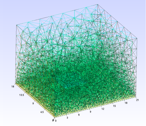
The extension of the geometry file is *.geo. A *.geo file is a text file that can be written and/or edited by hand using your favourite text editor. The file Box.geo is provided with this document and a number of comments (lines started with ) were added into the file to help the user. In the following, the geometry file Box.geo is explained step by step and the geometry itself can be seen in Figure 2.1. The user should pay particular attention to section 2.3.5 as it is one of the most important when creating a geometry.


2.3.1 Checking the consistency of the geometry
At any time, the user can visualise the geometry using the graphical interface of GMSH (Command 1) and check its consistency by running Command 2 in a terminal.
2.3.2 Parameters of the geometry
At the beginning of the file (see Code 1), several parameters are defined to provide a certain flexibility in the creation of the geometry.
-
•
If desired, the inner box can be rotated by an angle theta (in degree).
-
•
m_domain_top, m_domain_bottom, m_box, m_opening and m_source define the size of the elements in the final mesh (units are in meters). It should be noted that different size can be assigned in different part of the domain. Decreasing these values will increase the number of elements in the final mesh.
-
•
Finally, all the geometric parameters are defined, including the size and the position of the domain, the inner box and the openings. All units are in meters and the user can refer to Figure 2.1 to interpret each parameter.
2.3.3 Defining the geometry
General idea
Defining a geometry can be broken down into the following 6 steps:
-
•
Point: A point is defined as Point(idP)={x,y,z,m};, where x, y and z define the coordinates of the point having the ID idP. Each idP needs to be unique. m is the element size expected by the user near this point.
-
•
Line: A line is defined as Line(idL)={idP1,idP2};, where idL is the ID of the line starting at point idP1 and ending at point idP2. Each idL needs to be unique.
-
•
Line Loop: A line loop is defined as Line Loop(idLL)={idL1,idL2,idL3};, where idLL is the ID of the line loop composed by the lines having the IDs idL1, idL2 and idL3. Each idLL needs to be unique. Line loops are oriented and define how each lines are connected to each other to create a surface (at least 3 lines need to be provided). As line loops are oriented, a minus sign ‘-’ needs to be added in front of lines ID if needed (see line 101 in Code 2 for example).
-
•
Plane Surface: A plane surface is defined as Plane Surface(idS)={idLL};, where idS is the ID of the plane surface defined by the line loop having the ID idLL. Each idS needs to be unique. Note that surfaces need to be plane. The plane surfaces define the 2D surfaces that need to be meshed.
-
•
Surface Loop: A surface loop is defined as Surface Loop(idSL)={idS1,idS2, …};, where idSL is the ID of the surface loop created with the surfaces idS1, idS2, …. Each idSL needs to be unique. The surface loop groups all the surfaces defining a closed geometry (i.e a volume).
-
•
Volume: A volume is defined as Volume(idV)={idSL};, where idV is the ID of the volume defined by the surface loop having the ID idSL. Each idV needs to be unique. The volumes define the 3D space that needs to be meshed.
Useful trick
Even for simple geometries, it is easy to get confused with the IDs of points, lines, surfaces… These IDs can be seen on the graphical interface of GMSH for convenience. In a terminal, run gmsh Box.geo & to open the geometry. In GMSH, under Tools/Options/Geometry/Visibility/, the Point labels, Line labels and Surface labels can be easily displayed.
Example
In the example provided (Box.geo), the geometry of the domain is defined as in Code 2. The final Surface Loop and Volume are defined as shown in Code 4. The user can check, using any text editor, that the inner box, the opening and the source are defined like the domain. To help the user, the IDs of the points are given in Figure 2.2.


As shown in Code 3, if desired the inner box can be rotated, while keeping the external domain fixed.
2.3.4 Surfaces with holes
General idea
A Plane Surface with holes is defined as:
-
•
Plane Surface(idS)={idLL1,idLL2,idLL3 …};, where the surface with the ID idS is a plane surface defined by the line loop idLL1 minus the surfaces defined by the line loops idLL2, idLL3, …
This is particularly useful in two cases:
-
•
if a surface has actually a real hole (like the openings on the walls)
-
•
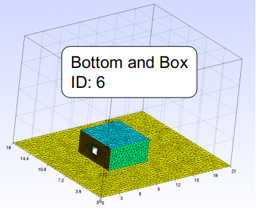
if different boundary conditions have to be assigned to different regions (in this example, we would like to assign a different boundary condition for the domain’s bottom and the box’s bottom, see section 2.3.5 for further details).
Example
Examining Box.geo file, one can see that some surfaces are not directly defined as Plane Surface if they contains holes: it is the case of the walls with openings and the bottom of the ground for example. As shown in Code 4 (line 410), the bottom of the domain is the surface defined by the line loop with ID 1006, minus the surface defined by the line loop with ID 3006 (corresponding to the bottom line loop defined by the external walls).
2.3.5 Defining the physical IDs
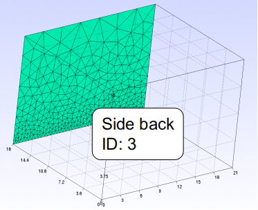
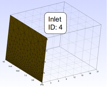
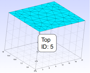
Surface IDs are used in Fluidity to mark different parts of the boundary of the computational domain so that different boundary conditions can be associated with them. In three dimensions, surface IDs are defined by assigning Physical Surface IDs in GMSH. The IDs are defined at the end of Box.geo as shown in Code 5. They are also summarised in the Figure 2.1.
2.3.6 Advice
It is recommended to add the line in Code 6 at the end of any *.geo file. This function removes all duplicate elementary geometrical entities (e.g., points having identical coordinates).
2.4 Mesh
2.4.1 Generating the mesh
Method
The extension of the mesh file is *.msh. To generate the mesh Box.msh associated with the geometry Box.geo, run the Command 3 in a terminal. The option -3 in Command 3 means that the geometry is in 3 dimensions (2 should be used instead if the geometry is 2D).
A file named Box.msh will be created. To visualise the mesh in GMSH, run the Command 4 in a terminal. In GMSH, under Tools/Options/Mesh/Visibility, the Surface faces or the Volume edges can be displayed as shown in Figure 2.3. By default, GMSH displays the Surface edges only. For convenience, the user can also choose to only display some part of the mesh. In GMSH, every surface and volume with respectively a Physical Surface or Physical Volume ID is listed under Tools/Visibility/ List browser. The user can select one or several surfaces at the same time to display in GMSH as done in Figure 2.3.


Common errors
The main common errors that occur when trying to generate the mesh are:
-
•
No tetrahedra in region idV: this happens mainly if the Surface Loop is not closed.
-
•
Found two facets intersect each other: two surfaces in Surface Loop are overlapping.
-
•
Found two duplicated facets: a surface in Surface Loop is defined twice.
2.4.2 Checking the consistency of the mesh
Method
At this stage, the mesh is created. Before running Fluidity, it is recommended to check if the generated mesh is consistent and suitable to run simulations. The check can be done in the following 3 steps:
- •
-
•
Step 2: The second step is to check if the mesh is consistent on a “GMSH” point of view. To this end, run the Command 5 in a terminal.
\colorbox{davysgrey}{\parbox{400pt}{\color{applegreen} \textbf{user@mypc}\color{white}\textbf{:}\color{codeblue}$\sim$\color{white}\$ gmsh -check Box.msh}}Command 5: Check the consistency of the mesh using GMSH tool. -
•
Step 3: The third step consists of using a Fluidity tool to test if the mesh is consistent on a “Fluidity” point of view. This can be done with the Command 6.
\colorbox{davysgrey}{\parbox{400pt}{\color{applegreen} \textbf{user@mypc}\color{white}\textbf{:}\color{codeblue}$\sim$\color{white}\$ checkmesh Box}}Command 6: Check the consistency of the mesh using Fluidity tool.
If all 3 steps suggested above are successful, then you are ready to run Fluidity simulations.
Common errors
Below are listed common errors that Command 5 and Command 6 can raise, as well as ideas on how to fix them:
-
•
From GMSH tool (Command 5)
-
–
duplicate vertex - duplicate elements: A surface is defined twice and different Physical Surface ID were assigned to them.
-
–
-
•
From Fluidity tool (Command 6):
-
–
Degenerate surface element found: if you have this error it is probably because you already had errors when generating the mesh. This is mainly due to the fact that the Surface Loop is not closed.
-
–
Degenerate volume element found: this error occurs if you have forgotten to define a Volume or to assign a Physical Volume ID to the volume.
-
–
Surface element does not exist in the mesh: A surface defined by a Physical Surface ID is not present in the Surface Loop.
-
–
WARNING: an incomplete surface mesh has been provided. This will not work in parallel. All parts of the domain boundary need to be marked with a (physical) surface id: The error is quite clear: each surface defining the Surface Loop has to have a Physical Surface ID and at least one surface does not.
-
–
Useful mesh statistics
2.5 Playing around
It is recommended that the user plays around with the parameters defined at the beginning of the file, to change the position and/or size of the openings for example. The user can also rotate the box if desired. Interested exercises would consist of modifying the Box.geo file to have the openings as “doors” instead of “windows”; or having the box in the middle of the domain instead of clipped to the ground. To create these geometries, the Box.geo will need a number of changes (the bottom surface will be defined differently for example), but the Box.geo provided can easily be used as a starting point.
Other options to experiment with are the parameters defining the elements size. Hence, the user can see the impact of reducing or increasing these values on the mesh aspect.
Chapter 3 Equations and numerical methods
The aim of this chapter is not to give extended overview of the equations and their implementations but only a brief idea of them. The reader can refer to [1, 3, 4, 5, 6] for more details.
3.1 Equations
3.1.1 Navier-Stokes and Large Eddy Simulation (LES)
The Large Eddy Simulation (LES) formulation implemented in Fluidity describes turbulent flows based on the filtered (three dimensional) incompressible Navier-Stokes equations (continuity of mass and momentum equation, see equation 3.1 and equation 3.2):
| (3.1) |
| (3.2) |
where is the resolved velocity (m/s), is the resolved pressure (Pa), is the fluid density (kg/m3), is the kinematic viscosity (m2/s) and is the anisotropic eddy viscosity (m2/s).
A novel component in the implementation of the standard LES equations within Fluidity is the anisotropic eddy viscosity tensor defined by equation 3.3.
| (3.3) |
is the Smagorinsky coefficient (usually taken equal to ), is the Smagorinsky length-scale which depends on the local element size and is the strain rate expressed as in equation 3.4.
| (3.4) |
where is the local strain rate defined by equation 3.5.
| (3.5) |
3.1.2 Advection-Diffusion equation
The transport of a scalar field (i.e, a passive tracer) having the unit is expressed using a classic advection-diffusion equation with a source term (equation 3.6).
| (3.6) |
where is the velocity vector (m/s), is the diffusivity tensor (m2/s) and represents the source terms (/s).
In the case where the scalar is the temperature in Kelvin, then the source term is expressed by equation 3.7
| (3.7) |
where is a power density expressed in W/m3.
In the case where the scalar is the species concentration in , then the source term is expressed by equation 3.8 or equation 3.9:
| (3.8) |
where is a mass flow rate expressed in and is the volume of the source in ;
| (3.9) |
where is a volumetric flow rate expressed in and is the volume of the source in .
3.1.3 Boussinesq approximation
Under certain conditions, one can assume that density does not vary greatly about a mean reference density, that is, the density at a position x can be written as:
| (3.10) |
where . Such an approximation is named the Boussinesq approximation. This assumption ignores density differences except when they are multiplied by , the acceleration due to gravity.
3.2 Numerical methods
3.2.1 Discretisation
For indoor-outdoor exchange simulations or urban environment simulations, the following discretisation are recommended:
-
•
Navier-Stokes equations: The Navier-Stokes equations, under the Boussinesq approximation, are solved using a continuous Galerkin finite element discretisation, while a Crank-Nicolson time discretisation approach is adopted.
-
•
Advection-diffusion equation: The advection-diffusion is solved using a control volume - finite element space discretisation, while a Crank-Nicolson time discretisation approach is adopted.
3.2.2 CFL number
To avoid crashes in simulations, the time step can be adaptive using a Courant-Friedrichs-Lewy (CFL) condition. This option allows the time step to vary throughout the run, depending on the CFL number. The maximum CFL number is set by the user as shown in Figure 5.2. The CFL condition is a necessary condition for convergence while solving certain partial differential equations and has the following form:
| (3.11) |
where C is the dimensionless CFL number, is the maximum CFL number given by the user, is the magnitude of the velocity (m/s), is the time step (s) and is the length interval, i.e taken as the edge element in the mesh (m).
It is commonly say that the maximum value of should be . However, in Fluidity, this value can be increased further (until 5-10) without convergence issues. However, it is recommended to start the simulations with a value of and then increase this value incrementally checking if the accuracy of the results are not affected. A too high CFL number might prematurely kill the turbulence.
3.2.3 Solver: PETSc
The solver used in Fluidity is the open-source solver toolbox PETSc. The user can refer to https://www.mcs.anl.gov/petsc/ for more information.
Chapter 4 Boundary and initial conditions
4.1 Introduction
This section shows examples of boundary conditions that can be used to set up a wide range of indoor simulations. They all rely on the geometry described previously which is a box with two openings in the middle of a wider computational domain. In this chapter, the fluid is air, with properties defined in Table 4.1. Gravity ( 9.81 m/s2) is taken into account. The Navier-Stokes equations, under the Boussinesq approximation, are solved for the fluid, while the advection-diffusion equation is solved for the heat transfers. The mesh and the time step are fixed and the simulations are run in serial.
Important note: The simulations with constant time steps work with the geometry file provided, i.e. if the element sizes have not been changed (see Section 2.3.2). If the mesh has been refined (i.e. the element size decreased), the simulations may crash. In that case, the time step has to be decreased under the option timestepping/timestep or the user can use an adaptive time step (option timestepping/adaptive_timestep) and use a CFL condition (see Section 3.2.2).
| Thermal Diffusivity | m2/s |
|---|---|
| Thermal Conductivity | W/m/K |
| Kinematic Viscosity | m2/s |
| Reference Density | kg/m3 |
| Thermal Expansion coefficient | K-1 |
| at K | |
| Specific Heat Capacity | J/kg/K |
In the next sections, different common and useful boundary conditions will be tested. The following will however remain fixed:
-
•
Outlet (Dirichlet boundary condition): A zero stress conditions is imposed at the outlet which sets . It must noted that at least one pressure boundary condition is required as a reference for Fluidity to run. See Section 4.6.
-
•
Sides and top of the domain (Dirichlet boundary condition): A perfect slip boundary condition is imposed on the sides and top of the domain which sets the normal component of velocity equal to zero.
-
•
Ground of the domain and walls (Dirichlet boundary condition): A zero velocity boundary condition is prescribed on the floor of the domain, the floor of the box and the walls of the box which sets the three components of velocity equal to zero. This boundary condition is discussed in details in Section 4.5.3.
Table 4.2 summarises the different simulations presented in the next sections.
|
Case
Nbr |
Time
Step |
Floor BC |
(m/s) |
Inlet
velocity (m/s) |
Section | |
|---|---|---|---|---|---|---|
| 1a | 1s | 293 K |
Dirichlet BC
K |
0 | 0 | 4.3.1 |
| 1b | 1s | 293 K |
Dirichlet BC
|
0 | 0 | 4.3.1 |
| 1c | 1s | 293 K |
Dirichlet BC
|
0 | 0 | 4.3.1 |
| 1d | 1s | 293 K |
Dirichlet BC
|
0 | 0 | 4.3.1 |
| 2a | 1s | 293 K |
Neumann BC
W/m2 |
0 | 0 | 4.3.2 |
| 2b | 1s | 293 K |
Neumann BC
W/m2 |
0 | 0 | 4.3.2 |
| 2c | 1s | 293 K |
Neumann BC
|
0 | 0 | 4.3.2 |
| 3 | 1s | 293 K |
Robin BC
°C W/m2/K |
0 | 0 | 4.3.3 |
| 4 | 1s |
Outside: 293 K
Inside: 298 K |
/ | 0 | 0 | 4.4 |
| 5a | 1s |
Outside: 293 K
Inside: 298 K |
/ | 1 | 1 | 4.5.1 |
| 5b | 1s |
Outside: 293 K
Inside: 298 K |
/ |
Log-
profile |
Log-
profile |
4.5.1 |
| 5c | 1s |
Outside: 293 K
Inside: 298 K |
/ | 1 |
Turbulent
inlet |
4.5.2 |
| 5d | 1s |
Outside: 293 K
Inside: 298 K |
/ |
Log
profile |
Turbulent
inlet |
4.5.2 |
4.2 Quick start
Running a simulation
Running a simulation with Fluidity consists of the following steps:
-
•
Step 1: Set up the Fluidity options in 3d_Case.flml using the graphical interface Diamond running diamond 3d_Case.flml &
-
•
Step 2: Run Fluidity using <<FluiditySourcePath>>/bin/fluidity -l -v3 3d_Case.flml &
-
•
Step 3: Visualise the Fluidity log file during the simulation using the command tail -f fluidity.log-0 in a terminal.
-
•
Step 4: Open the Fluidity error file using the command gedit fluidity.err-0 & in a terminal.
Command 1 is the basic command line to run a simulation with Fluidity. One can notice two options:
-
•
-l: This option writes the terminal log and errors in the files fluidity.log-0 and fluidity.err-0, respectively, instead of writing them directly in the terminal.
-
•
-v3: This is the degree of verbosity that the user wants. The user can choose between -v1, -v2 and -v3, where -v1 will be less verbose than -v3.
Killing a simulation
At any time, to kill a simulation, the following can be done in a terminal:
-
•
Run the command top. All the processes currently running on the machine are listed, including the Fluidity simulations. Note the ProcID that you want to kill, then press the key q to quit.
-
•
As the user can have several simulations running in different folders, the command pwdx ProcID can be use to determine where the ProcID is currently running. This command will provide the path where the simulation was launched.
-
•
Once the user is sure that the simulation to kill has the ID ProcID, then the command kill -9 ProcID can be run in a terminal to kill the simulation.
4.3 Thermal boundary conditions
4.3.1 Dirichlet boundary condition: Constant temperature
Constant floor temperature
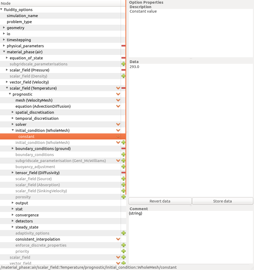
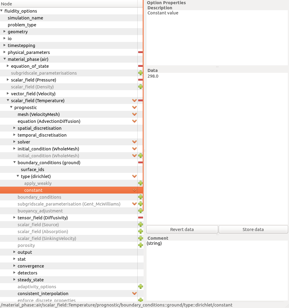
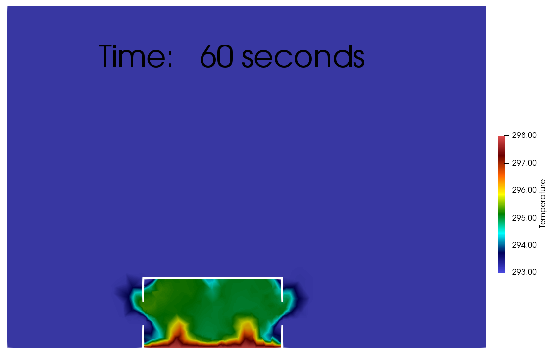
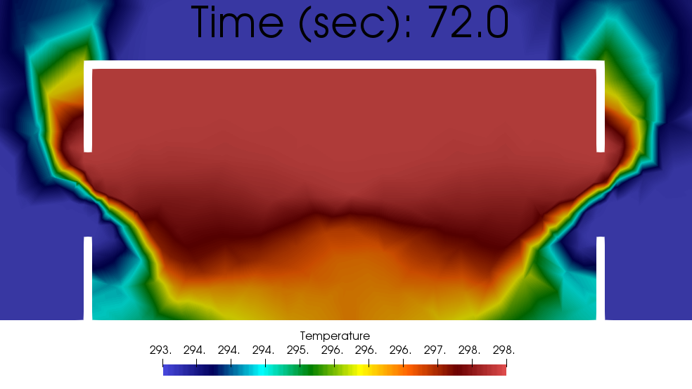
In 3dBox_Case1a.flml, the floor of the box is set to a constant temperature of 298K (Figure 4.1(b)) using a Dirichlet boundary condition. The initial and the ambient temperatures are set to 293 K (Figure 4.1(a)). The initial and inlet velocity are set to m/s (Figure 4.1(c) and Figure 4.1(d)). This simulation can be run using the command:
A snapshot of the result obtained at 60 s is shown in Figure 4.2. Go to Chapter 10 to learn how to visualise the results using ParaView.

Floor temperature as a function of space and/or time: python script
In some cases, the user might want to prescribe a Dirichlet boundary that is space and/or time dependent. This can be done in Diamond using a python script. The following examples show how to prescribe these kinds of boundary conditions.
-
•
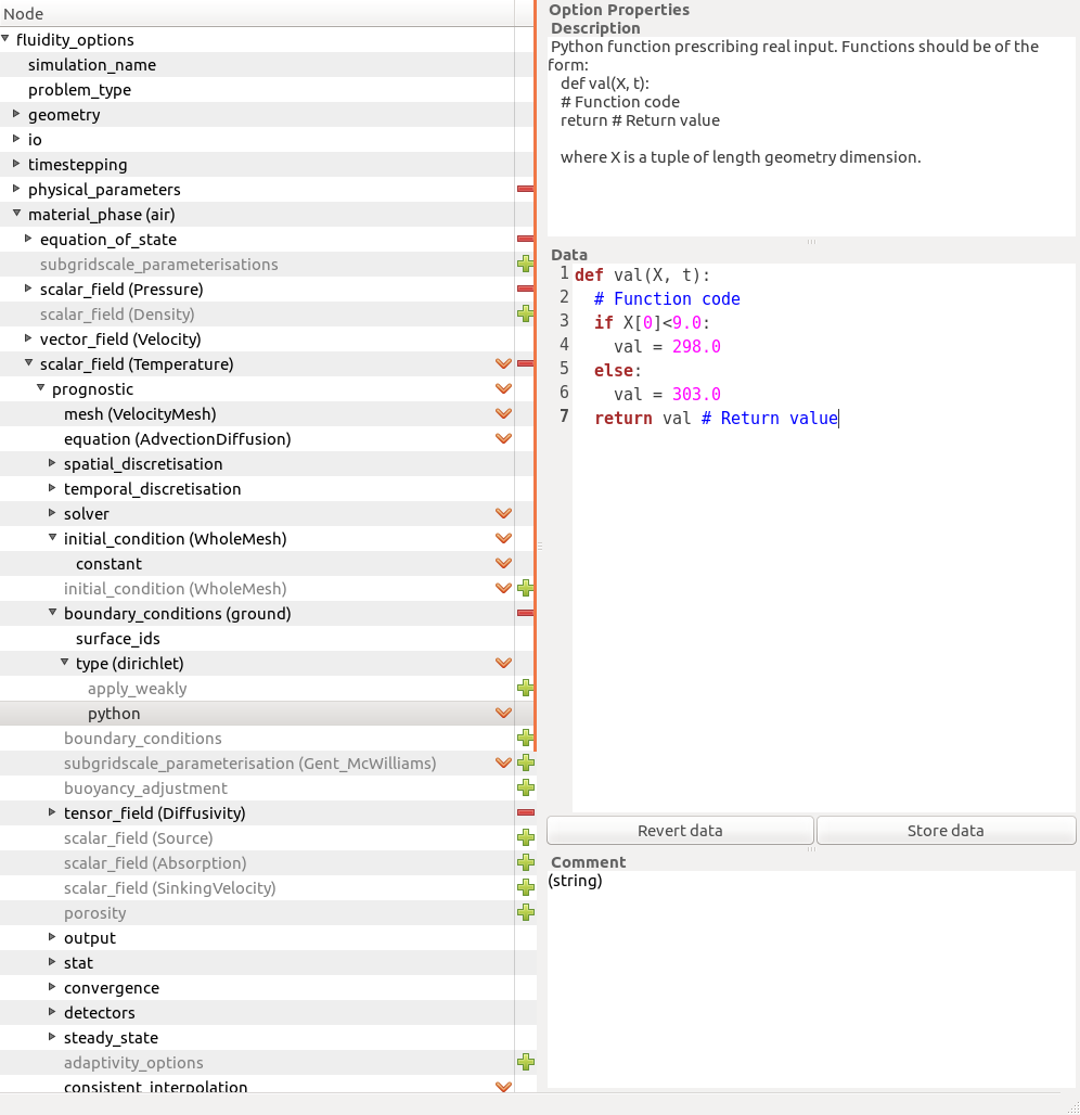
Space dependent boundary condition: In 3dBox_Case1b.flml, as shown in Figure 4.3(a), the python script Code 1 is used.
1def val(X, t):2 # Function code3 if X[0]<9.0:4 val = 298.05 else:6 val = 303.07 return val # Return valueCode 1: Space dependent Dirichlet boundary condition for temperature. -
•
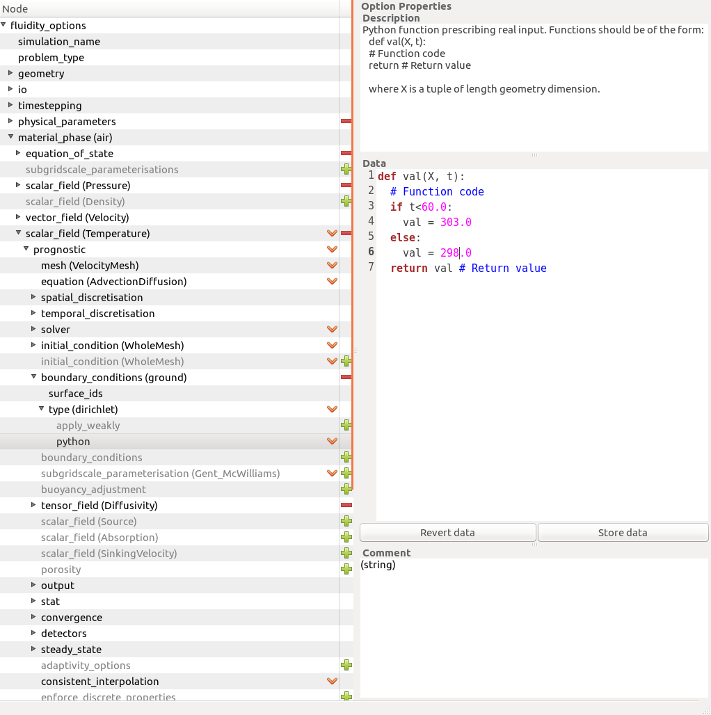
Time dependent boundary condition: In 3dBox_Case1c.flml, as shown in Figure 4.3(b), the python script Code 2 is used.
1def val(X, t):2 # Function code3 if t<60.0:4 val = 303.05 else:6 val = 298.07 return val # Return valueCode 2: Time dependent Dirichlet boundary condition for temperature. -
•
Space and time dependent boundary condition: In 3dBox_Case1d.flml, as shown in Figure 4.3(c), the python script Code 3 is used.
1def val(X, t):2 # Function code3 if t<60.0:4 if X[1] < 9.0:5 val = 298.06 else:7 val = 303.08 else:9 if X[1] < 9.0:10 val = 303.011 else:12 val = 298.013 return val # Return valueCode 3: Space and time dependent Dirichlet boundary condition for temperature.

These examples can be run using the commands:
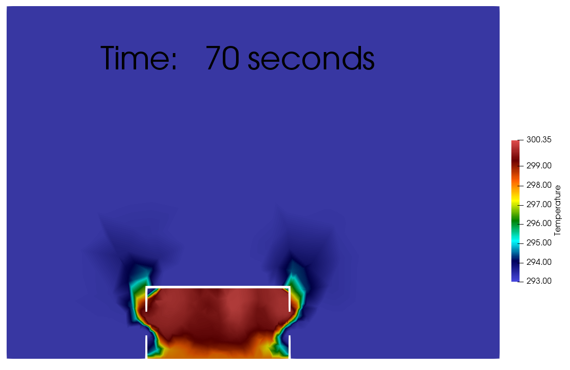
Snapshots of the results obtained from these three simulations are shown in Figure 4.4. Go to Chapter 10 to learn how to visualise the results using ParaView.

4.3.2 Neumann boundary condition: Heat flux
Heat flux from the ground
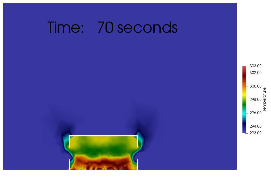
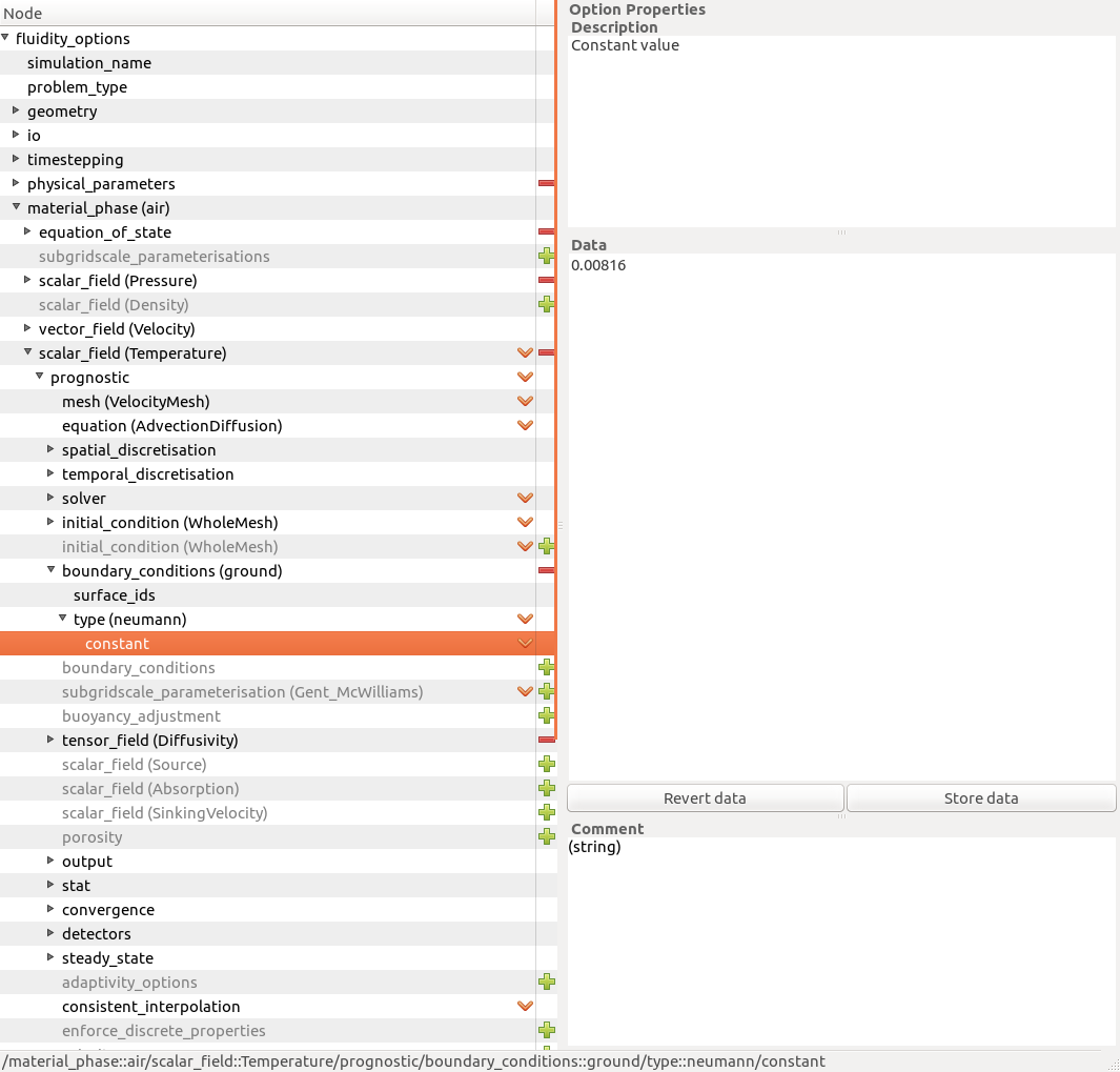
Case 3dBox_Case2a.flml is similar to the previous one, except a heat flux is now applied at the bottom, effectively changing the Dirichlet boundary condition to a Neumann one as shown in Figure 4.5(a). The ambient and the initial temperatures are set to 293 K and is set equal to m/s. In Fluidity, the value of the heat flux, specified in Diamond, is given by equation 4.1:
| (4.1) |
where (Km/s) is the value that needs to be set into Diamond, (W/m2) is the actual heat flux that the user wants to prescribe, (kg/m3) is the reference density and (J/kg/K) is the heat capacity of the fluid.
In example 3dBox_Case2a.flml, the heat flux is equal to 10 W/m2, hence the value is set up in Diamond as shown in Figure 4.5(a). The 10 W/m2 heat flux is applied to the box’s floor having a surface equal to m2: the flux is then equal to W.


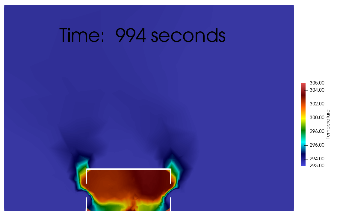
This example can be run using the command:
A snapshot of the result obtained at 994 s is shown in Figure 4.6(a). Go to Chapter 10 to learn how to visualise the results using ParaView.

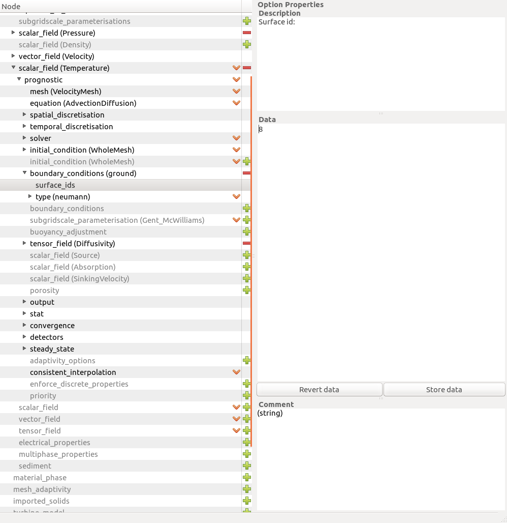
Heat flux from the source only
Using the physical IDs previously defined (see Section 2.3.5), the heat flux boundary condition can be changed to include only a section of the floor, defined as the source. Based on Section 2.3.5, the ID of the floor of the box (without the source) is 7 and the ID of the source only is 8. In the previous example 3dBox_Case2a.flml, the surface IDs, where the Neumann boundary condition were applied, are 7 (the floor) and 8 (the source) (see Figure 4.5(b)): in that case, the heat flux is applied everywhere on the floor. In example 3dBox_Case2b.flml, the surface ID where the Neumann boundary condition is applied is 8 only (the source) (see Figure 4.5(c)). Therefore the heat flux is applied at the source only.
In case 3dBox_Case2b.flml, the initial and the ambient temperatures are set to 293 K and is set equal to m/s. The heat flux applied at the source is equal to 1000 W/m2, hence set up in Diamond is equal to 0.8163 according to equation 4.1. The surface of the heat source is m2: the flux applied at the source is then equal to 40 W.
This example can be run using the command:
Heat flux as a function of space or time: python script
In some cases, the user might want to prescribe a Neumann boundary that is space and/or time dependent. This can be done in Diamond using a python script as shown in Figure 4.5(d).
In example 3dBox_Case2c.flml, the python script Code 4 is used. Note that in this example, the choice was made to calculate the heat flux directly in the python script.
This example can be run using the command:
4.3.3 Robin boundary condition
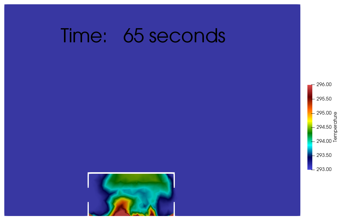
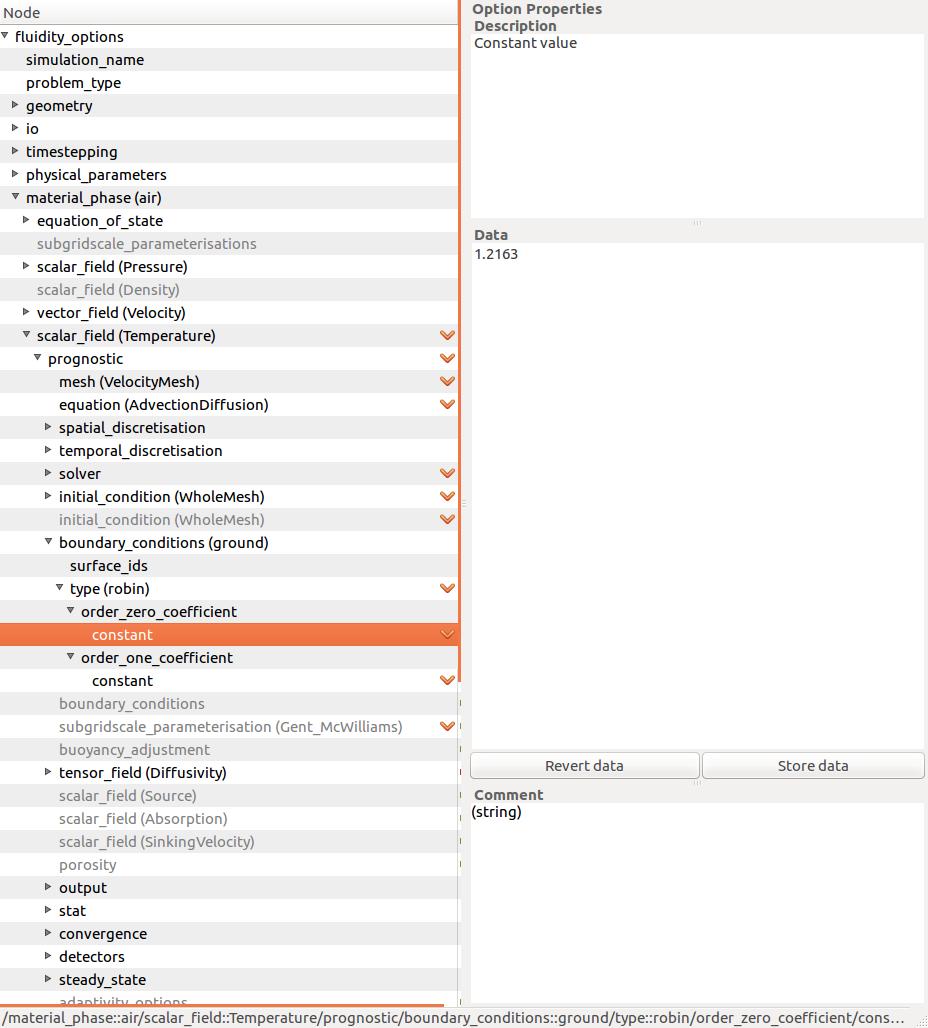
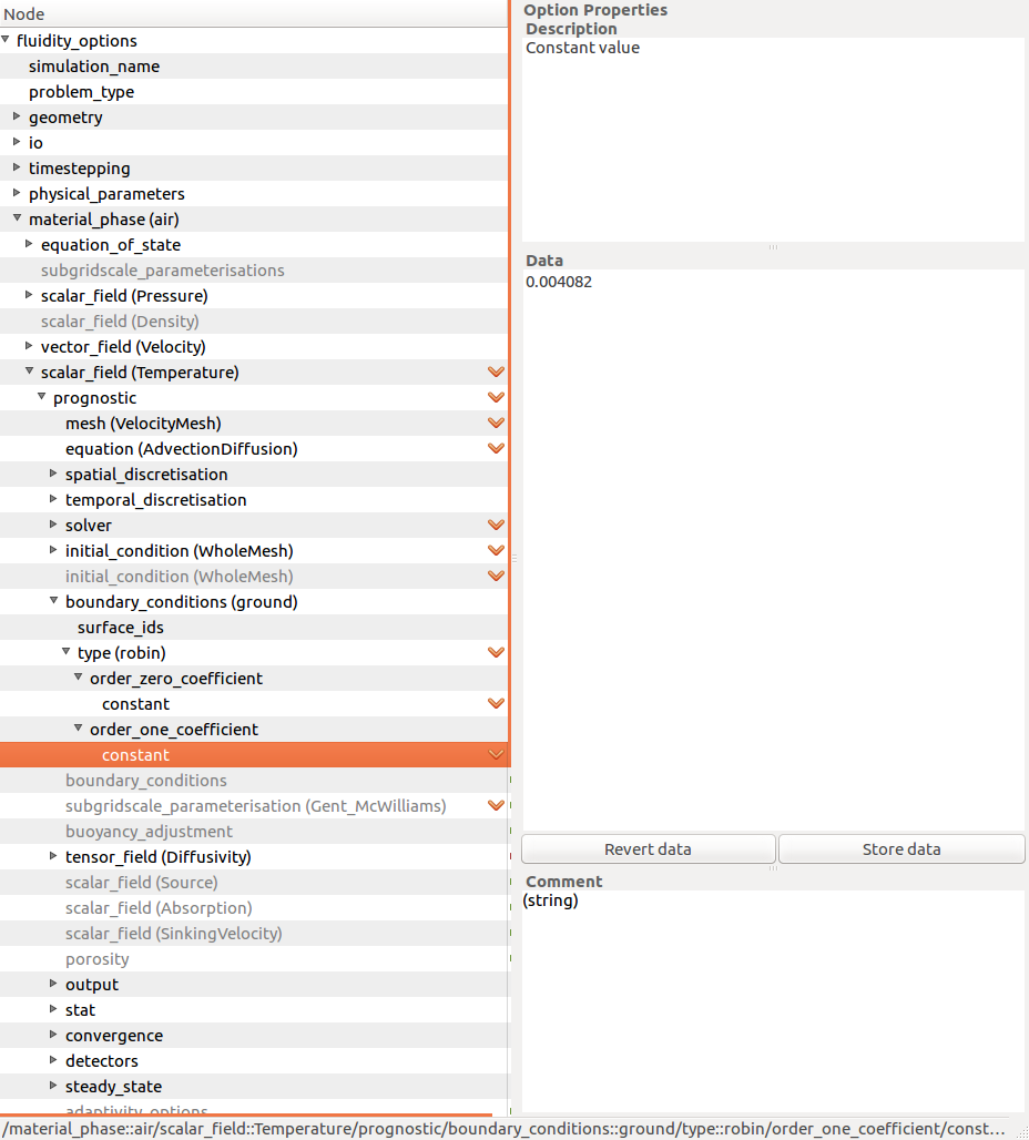
In example 3dBox_Case3.flml, a Robin boundary condition (equation 4.2) is applied between the box’s floor and the air as shown in Figure 4.7. Generally this boundary condition is used to model the heat exchange by convection between a fluid and a solid surface.
| (4.2) |
where is the thermal diffusivity (m2/s) of the fluid, is the convective heat transfer coefficient (W/m2/K) and is the ground temperature (K).
In Fluidity, the Robin boundary condition is specified using the equation 4.3.
| (4.3) |
| (4.4) |
| (4.5) |
where is in Km/s and is in m/s. Note that if is equal to 0, then the Robin boundary condition leads to a Neumann boundary condition.
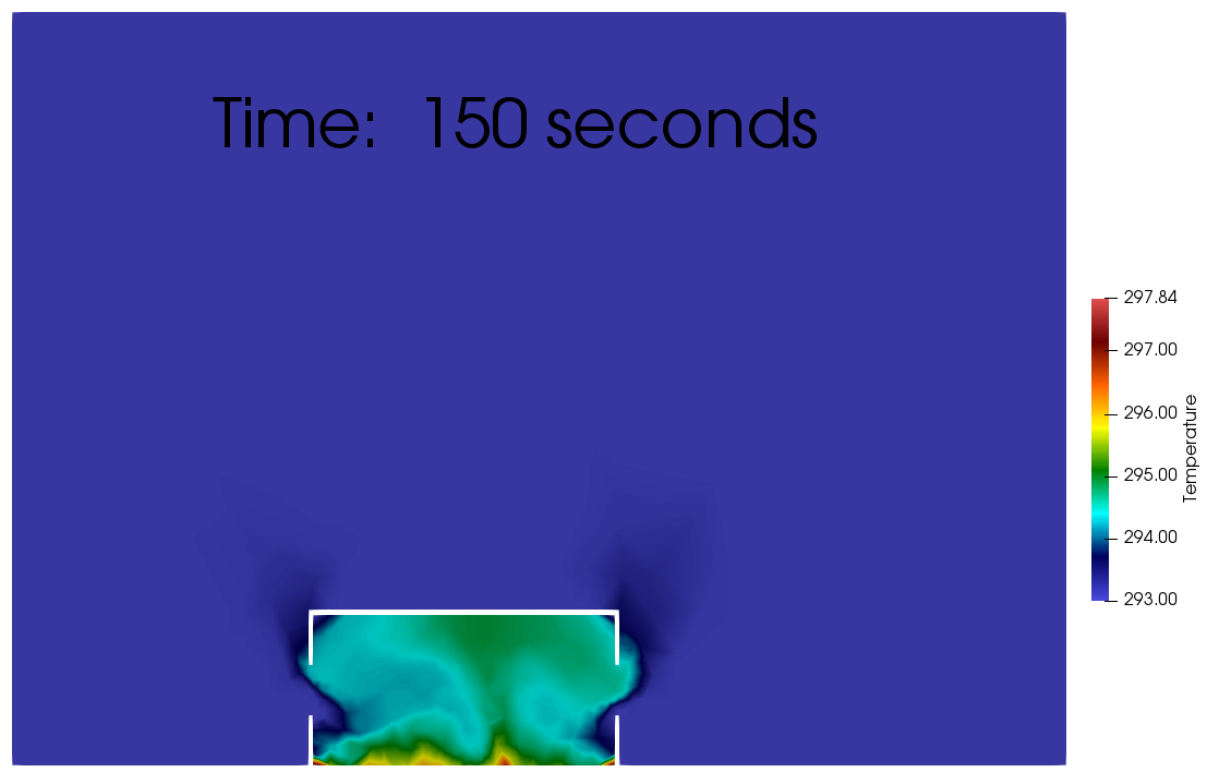
In example 3dBox_Case3.flml, the heat transfer coefficient between the ground and the air is assumed to be equal to 5 W/m2/K and the ground temperature is taken equal to 298 K. Hence, the value of and are equal to 1.2163 Km/s and 0.004082 m/s, respectively as shown in Figure 4.7. The initial temperature is set to 293 K and is set equal to m/s.
This example can be run using the command:
A snapshot of the result obtained at 150 s is shown in Figure 4.8. Go to Chapter 10 to learn how to visualise the results using ParaView.
4.4 Initial conditions for temperature
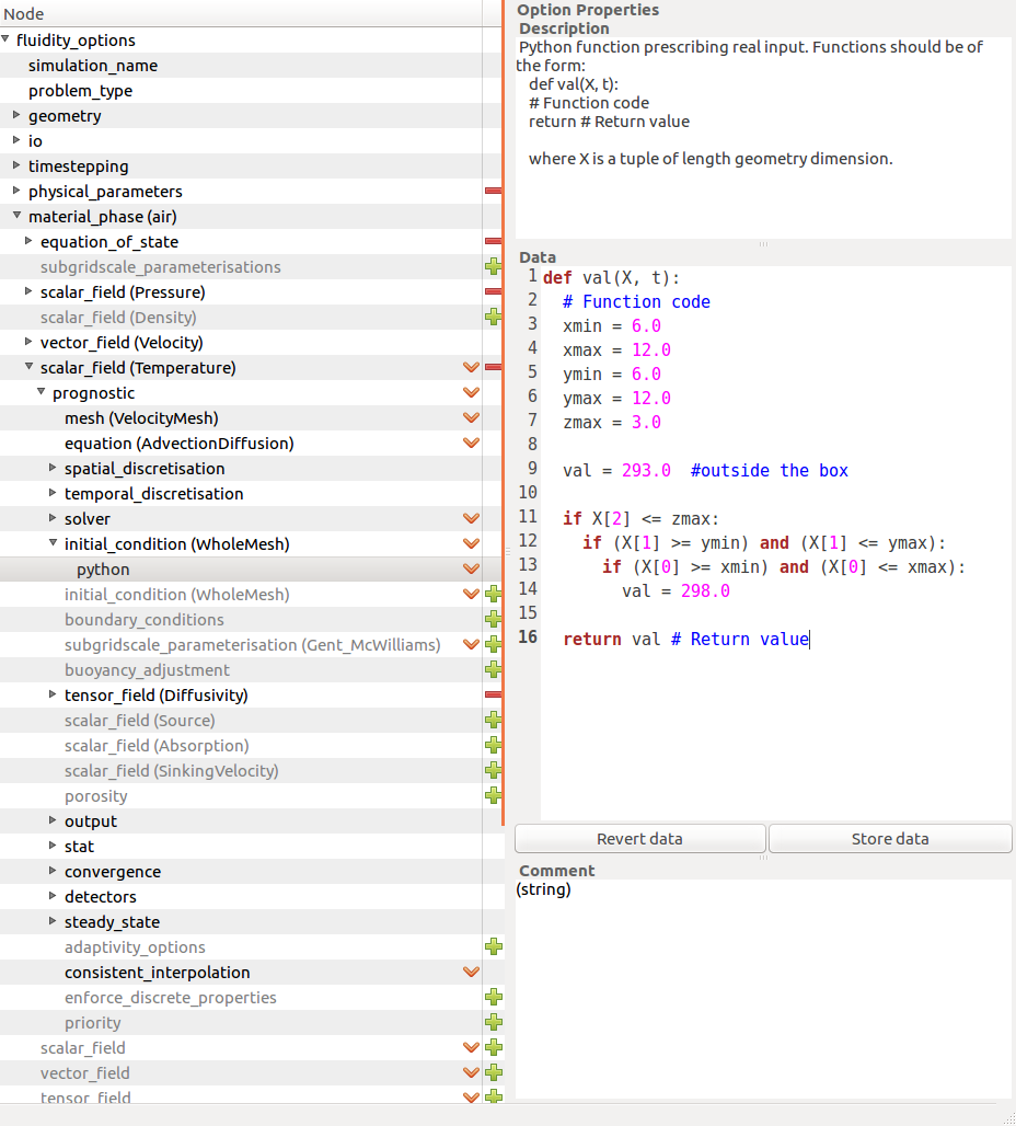
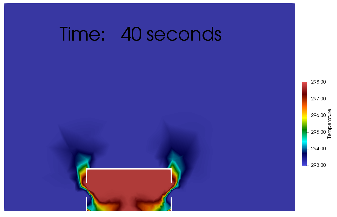
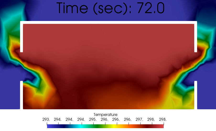
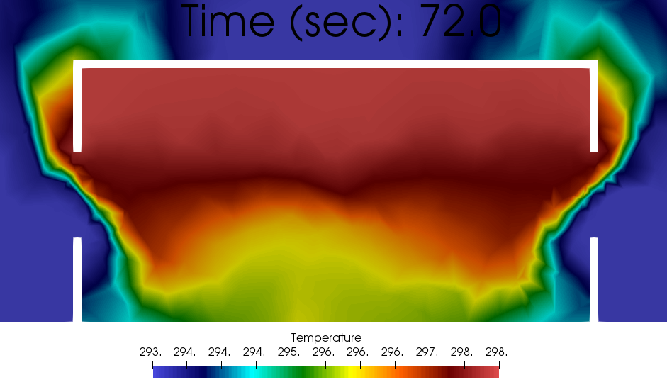
The initial temperature can be set using a python script to prescribe different initial values in different regions. In example 3dBox_Case4.flml, the interior of the box is set to 298 K while the outside remains at ambient temperature, i.e. 293 K. The python script in Code 5 is used as shown in Figure 4.9. No particular thermal boundary condition is prescribed for the floor of the box and is set to m/s.
This example can be run using the command:
A snapshot of the result obtained at 40 s is shown in Figure 4.10. Go to Chapter 10 to learn how to visualise the results using ParaView.
4.5 Velocity boundary conditions
4.5.1 Dirichlet boundary condition: Constant and uniform inlet wind
Uniform inlet velocity
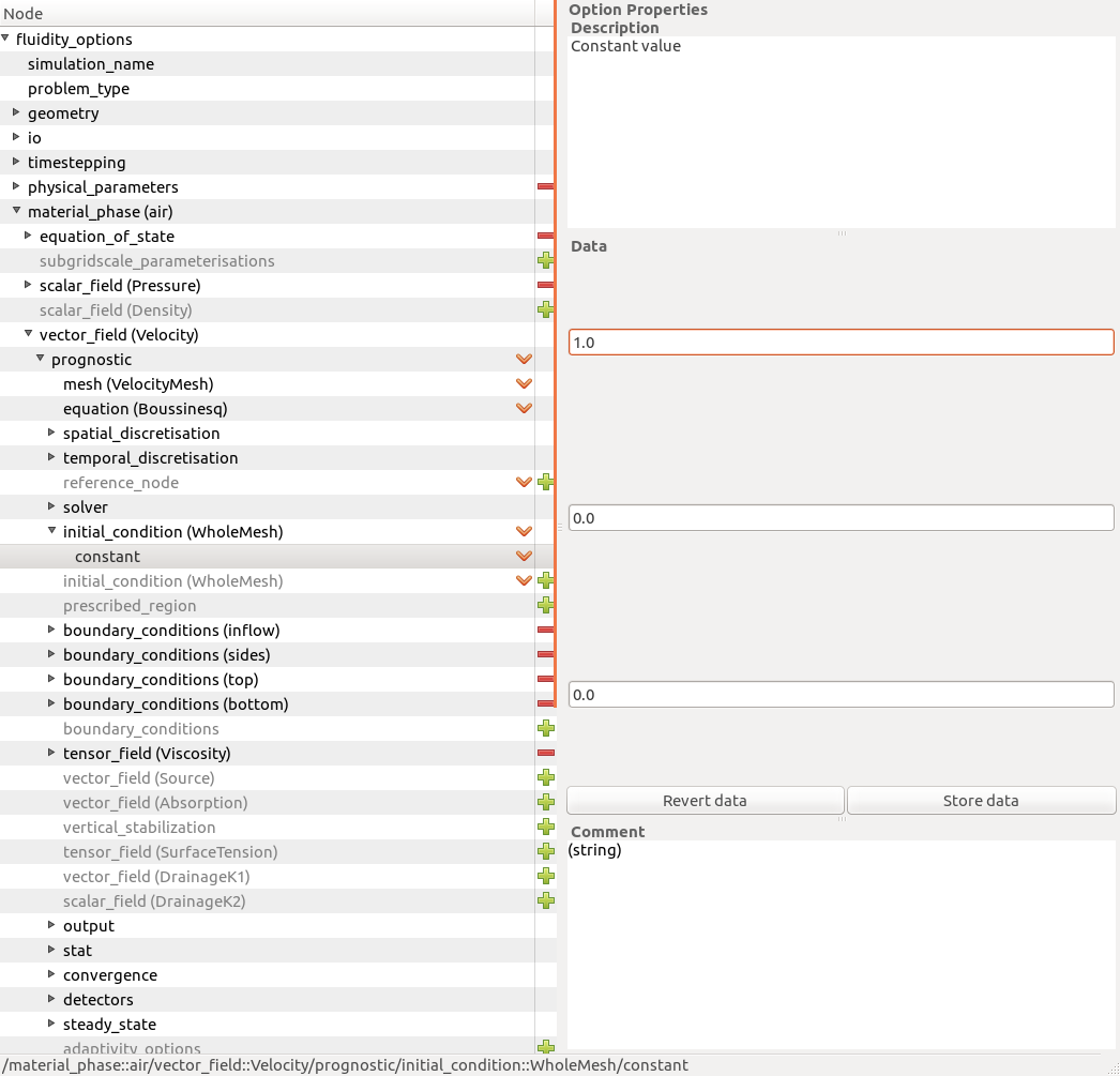
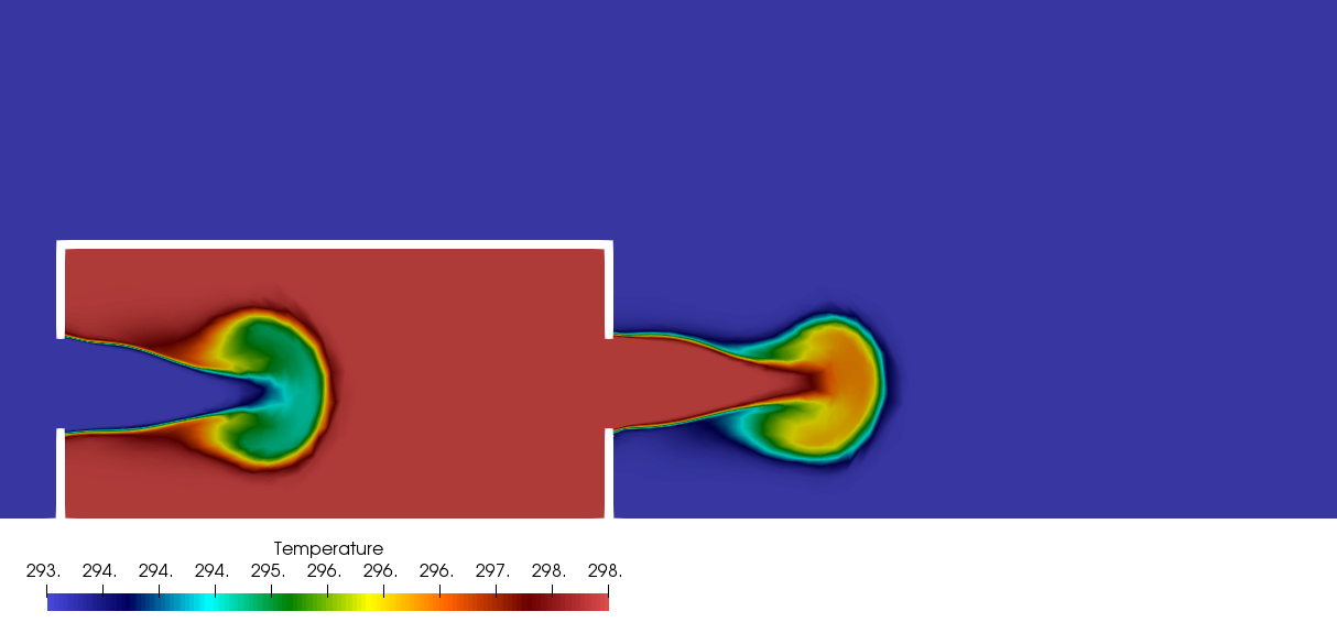
In addition to setting boundary or initial values of temperature, the boundary condition for velocity can also be specified. In example 3dBox_Case5a.flml, the initial and inlet velocities are set to m/s (Figure 4.11) and the interior of the box is set to 298 K while the outside remains at ambient temperature 293 K (Code 5). The time step is kept equal to 1 s in this example. However, the results of the first 10 time steps are not totally accurate. To avoid this, a value of 0.01 s is recommended.
This example can be run using the command:
A snapshot of the result obtained at 50 s is shown in Figure 4.12(a). Go to Chapter 10 to learn how to visualise the results using ParaView.
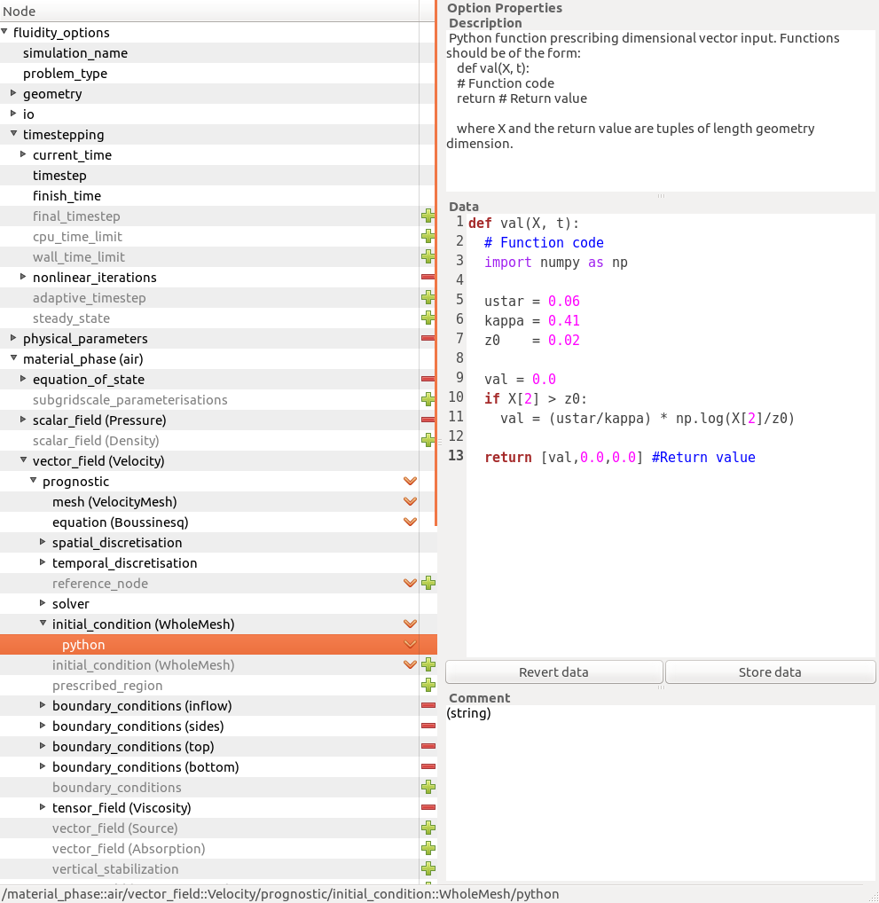
Prescribing a velocity profile: python script
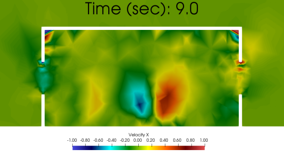
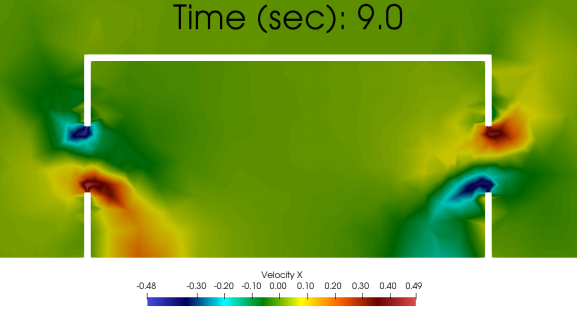
In example 3dBox_Case5b.flml, the -component of the initial and inlet velocity are set using a log-profile and the python scripts in Code 6 and Code 7 are used (Figure 4.13).The interior of the box is set to 298 K while the outside remains at ambient temperature 293 K (Code 5).

This example can be run using the command:
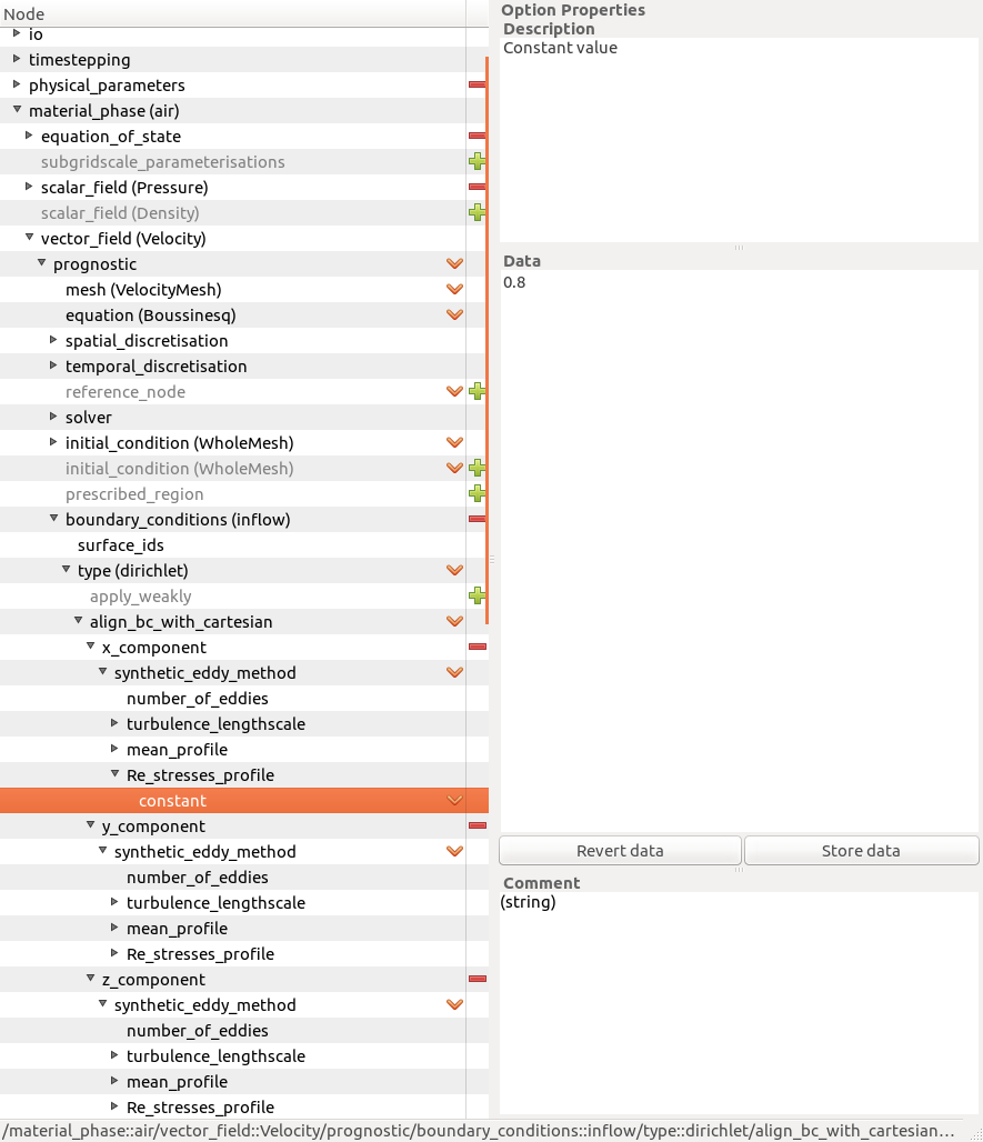
4.5.2 Synthetic eddy method: Turbulent inlet velocity
Constant values
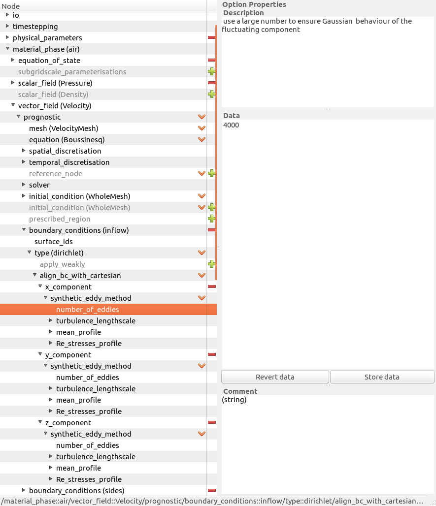
Finally, the last interesting velocity boundary condition is called the Synthetic eddy method and mimics a turbulent inlet velocity. For more details, the user can refer to [5]. This boundary condition is used to reproduced the behaviour of the atmospheric boundary layer and the 4 following variables need to be defined by the user for each velocity component:
-
•
Number of eddies: this number has to be large enough to ensure the Gaussian behaviour of the fluctuating component. Usually this value is taken to be .
-
•
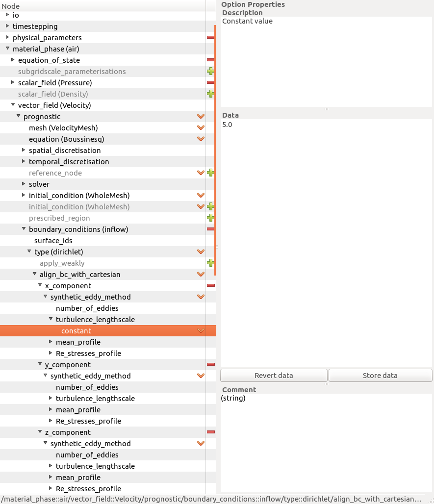
Turbulence lengthscale: the turbulence lengthscale is in meters and is defined by equation 4.6.
-
•
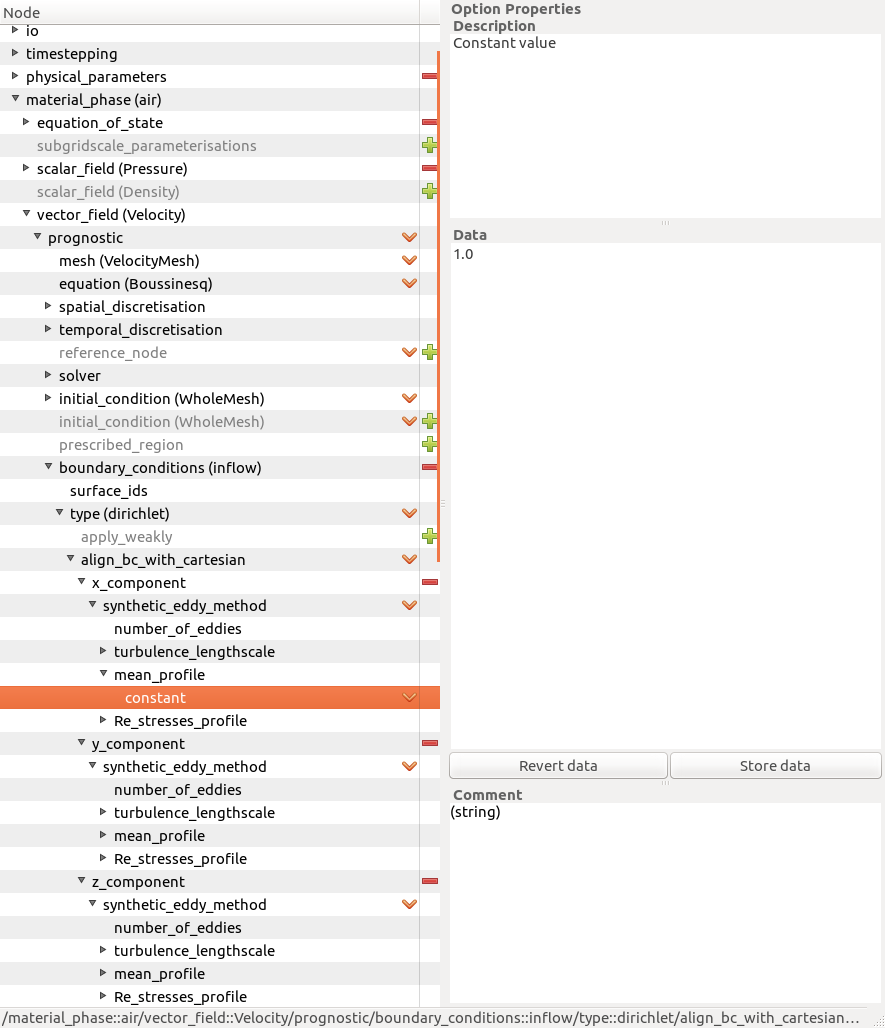
Mean profile: the mean velocity profiles of each velocity component in m/s.
-
•
Reynolds stresses profile: the Reynolds stresses profile of the components , and (in m2/s2) are prescribed assuming that the remaining stresses are negligible as in equation 4.7.
| (4.6) |
| (4.7) |
In example 3dBox_Case5c.flml, the interior of the box is set to 298 K while the outside remains at ambient temperature 293 K (Code 5). The initial velocity and the inlet velocity are set to m/s. The number of eddies is taken as and the turbulence lengthscale is equal to m. The -component of the Reynolds stresses is taken to be to , while and are equal to . For brevity, the options set up for the -component only are shown in Figure 4.14.
This example can be run using the command:
Using python scripts
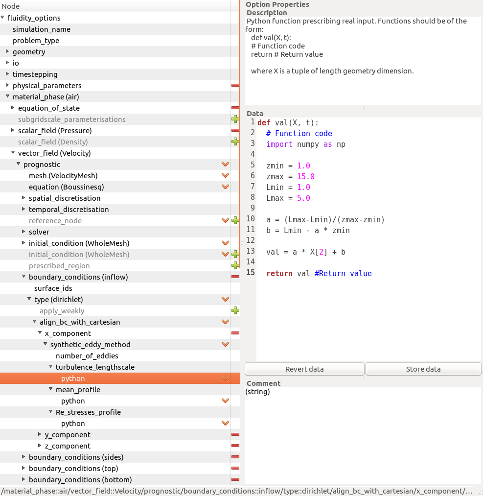
The initial velocity, the turbulence lengthscale, the mean velocity and the Reynolds stresses profiles can also be prescribed using python scripts if the user wants to use real profiles found in literature. In example 3dBox_Case5d.flml, the interior of the box is set to 298 K while the outside remains at ambient temperature 293 K (Code 5). The initial velocity is prescribed using Code 6. The turbulent inlet options are defined as follows (see also Figure 4.15):
-
•
Turbulence lengthscale: Assuming a linear relationship between the lengthscale and the height, the python script in Code 8 is used for the three velocity components as shown in Figure 4.15(a).
1def val(X, t):2 # Function code3 import numpy as np45 zmin = 1.06 zmax = 15.07 Lmin = 1.08 Lmax = 5.0910 a = (Lmax-Lmin)/(zmax-zmin)11 b = Lmin - a * zmin1213 val = a * X[2] + b1415 return val #Return valueCode 8: Python script to prescribe a turbulence lengthscale profile. -
•
Mean velocity: Assuming a log-profile, the python script in Code 7 is prescribed to the -component of the velocity, while m/s is prescribed to the and -components.
-
•
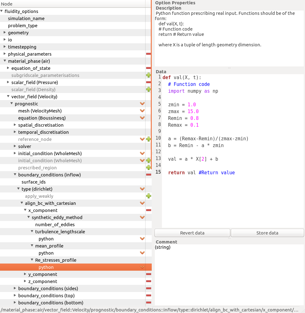
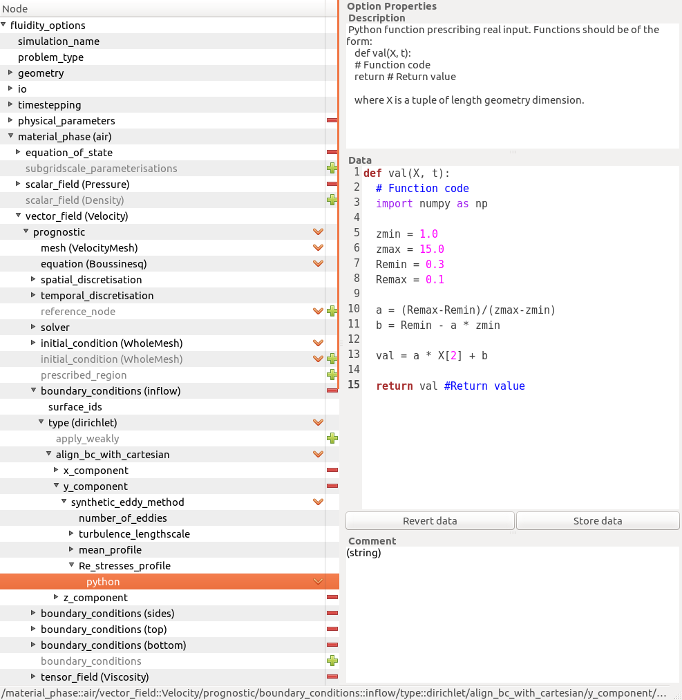
Reynolds Stresses: The -component of the Reynolds stresses are prescribed using the python script in Code 9 (Figure 4.15(b)). The and components of the Reynolds stresses is prescribed using the python script in Code 10 (Figure 4.15(c)). A linear relationship between the Reynolds stresses and the height is assumed.
1def val(X, t):2 # Function code3 import numpy as np45 zmin = 1.06 zmax = 15.07 Remin = 0.88 Remax = 0.1910 a = (Remax-Remin)/(zmax-zmin)11 b = Remin - a * zmin1213 val = a * X[2] + b1415 return val #Return valueCode 9: Python script to prescribe the Reynolds stresses . 1def val(X, t):2 # Function code3 import numpy as np45 zmin = 1.06 zmax = 15.07 Remin = 0.38 Remax = 0.1910 a = (Remax-Remin)/(zmax-zmin)11 b = Remin - a * zmin1213 val = a * X[2] + b1415 return val #Return valueCode 10: Python script to prescribe the Reynolds stresses and .
This example can be run using the command:
4.5.3 Dirichlet boundary condition on solids
Note: This section is particularly important and it is recommended to read it carefully. This section is also summarised in Section 8.4 due to its importance. The option align_bc_with_surface in the Dirichlet type boundary condition is not well-implemented in Fluidity and not always work properly. This section describes in details in which case it works or not. In any case, this option should be avoided if possible. The simulations presented in that section are based on 3dBox_Case4.flml and are summarised in Table 4.3.
|
Case
Nbr |
BC type | From |
Aligned
with |
BCs aligned
with surface |
Work? |
|---|---|---|---|---|---|
| 4 | Dirichlet: No-slip | Strong | Cartesian | N/A | YES |
| 13a | Dirichlet: No-slip | Strong | Surface | 1 | YES |
| 13b | Dirichlet: No-slip | Strong | Surface | 2 | NO |
| 13c | Dirichlet: No-slip | Weak | Cartesian | N/A | YES |
| 13d | Dirichlet: No-slip | Weak | Surface | 1 | YES |
| 13e | Dirichlet: No-slip | Weak | Surface | 2 | YES |
| 13f | Dirichlet: Slip | Strong | Surface | 1 | YES |
| 13g | Dirichlet: Slip | Weak | Cartesian | N/A | YES |
| 13h | Dirichlet: Slip | Weak | Surface | 1 | NO |
| 13i | No normal flow: Slip | Weak | N/A | N/A | YES |
Boundary condition align_bc_with_cartesian or align_bc_with_surface?
It exists two options available to apply a Dirichlet boundary condition in Fluidity:
-
•
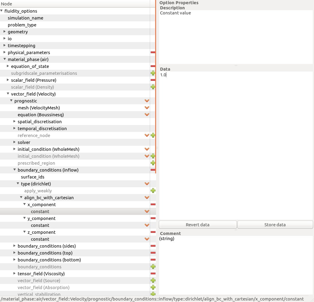
align_bc_with_cartesian: the three components of the velocity are assigned.
-
•
align_bc_with_surface: the normal and the two tangential components of the velocity are assigned.
The second option can be really useful when the surfaces of the geometry are not aligned with Cartesian coordinates system for very complex geometry. However, this functionality does not always work properly in Fluidity as detailed in the following:
-
•
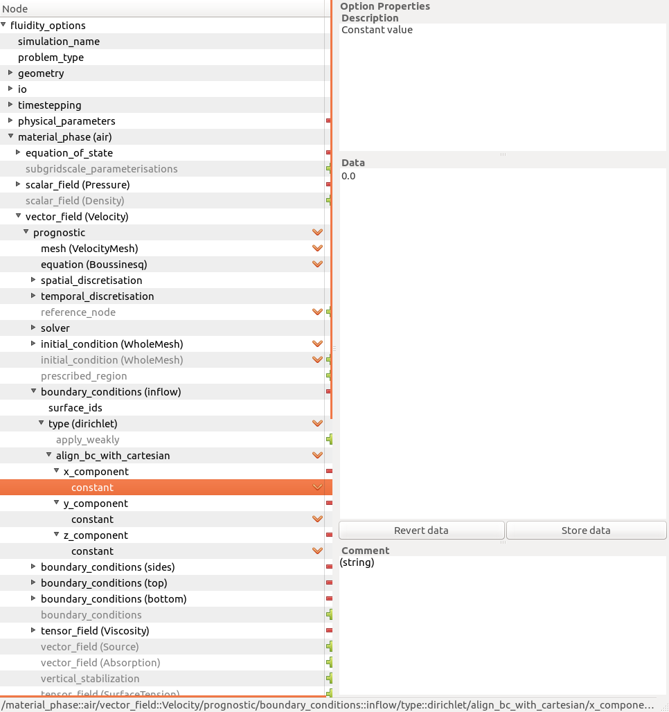
Example 3dBox_Case4.flml uses the option align_bc_with_cartesian to apply a no-slip boundary condition (the three components , and of the velocity are equal to zero) on the solid surfaces.
-
•
Example 3dBox_Case13a.flml is a replicate of example 3dBox_Case4.flml, excepted that the velocity boundary condition on the solid surfaces is now applied using the align_bc_with_surface option, i.e. the normal and the two tangential components of the velocity are now equal to zero.
-
Examples 3dBox_Case4.flml and 3dBox_Case13a.flml run correctly and give the same results - that was actually expected…
-
-
•
In 3dBox_Case13b.flml, the no-slip boundary condition align_bc_with_surface is now dissociated into two no-slip boundary conditions align_bc_with_surface: one for the ground of the domain and the walls; and one for the ground of the box only.
-
If the user runs example 3dBox_Case13b.flml, the simulation will crash and the error in Command 13 will be raised.
-
Unfortunately, if several strong boundary conditions (see next section for discussion about the strong form) align_bc_with_surface are really wanted, there is not tricks to avoid this error in Fluidity. Only one align_bc_with_surface Dirichlet boundary condition strongly applied is allowed by Fluidity, which can be problematic when dealing with complex geometries.
Boundary condition applied strongly or weakly?
The only way to avoid the error previously described (when more than one align_bc_ with_surface no-slip Dirichlet boundary condition is used) is to apply the boundary conditions weakly.
It is to be noted that when boundary conditions are applying weakly, the discrete solution will not satisfy the boundary condition exactly. Instead the solution will converge to the correct boundary condition along with the solution in the interior as the mesh is refined. An alternative way of implementing boundary conditions is to strongly imposed boundary conditions. Although this guarantees that the Dirichlet boundary condition will be satisfied exactly, it does not at all mean that the discrete solution converges to the exact continuous solution more quickly than it would with weakly imposed boundary conditions. Strongly imposed boundary conditions may sometimes be necessary if the boundary condition needs to be imposed strictly for physical reasons. Unlike the strong form of the Dirichlet conditions, weak Dirichlet conditions do not force the solution on the boundary to be point-wise equal to the boundary condition.
If boundary conditions are applied weakly, then the following options need to be turned on in Diamond:
-
•
Under the Pressure field: spatial_discretisation/continuous_galerkin/
integrate_continuity_by_parts -
•
Under the Velocity field: spatial_discretisation/continuous_galerkin/
advection_terms/integrate_advection_by_parts
Examples 3dBox_Case13c.flml, 3dBox_Case13d.flml and 3dBox_Case13e.flml use a no-slip boundary condition applied weakly. The time-step was reduce to second to avoid divergence of the simulation and the options integrate_*_by_parts are turned on.
-
•
Example 3dBox_Case13c.flml is equivalent to 3dBox_Case4.flml, excepted that the velocity boundary condition on solid surfaces is now applied weakly instead of strongly, still using align_bc_with_cartesian.
-
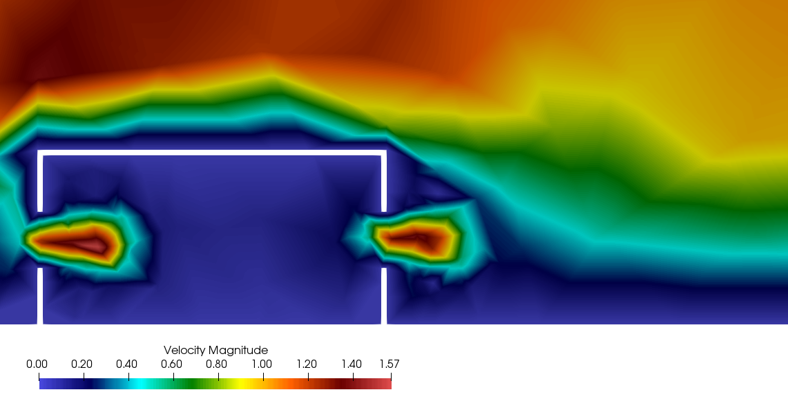
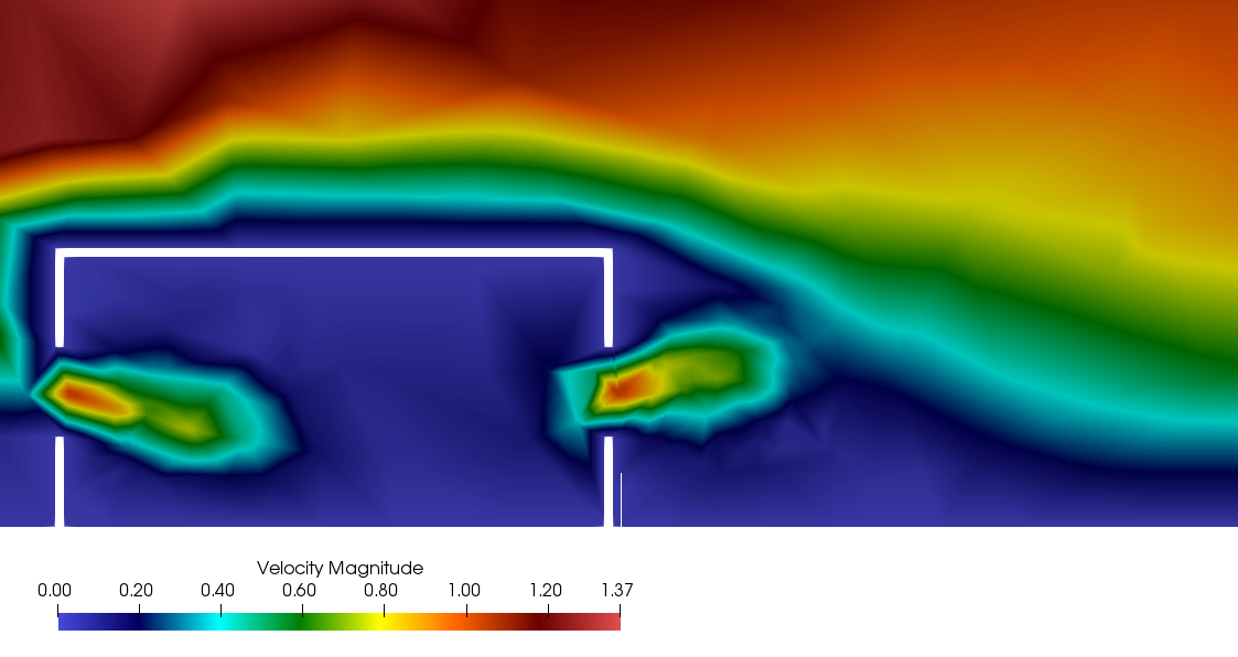
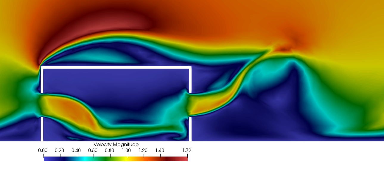
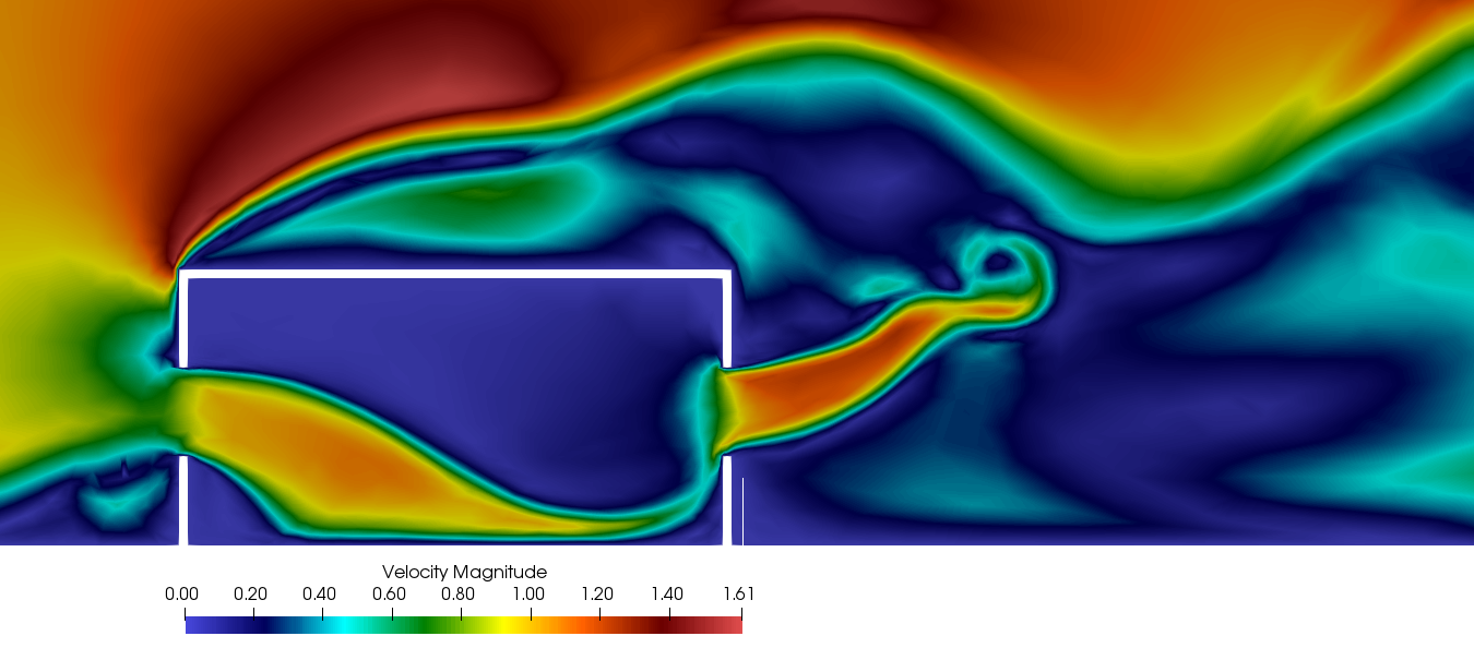
As shown in Figure 4.16, the velocity is not equal to zero on solid walls for the reason explained above, i.e. because the boundary condition is applied weakly.
-
-
•
Example 3dBox_Case13d.flml is the same than 3dBox_Case13c.flml, excepted that the velocity boundary condition on solid surfaces, still applied weakly, is now align_bc_with_surface.
-
The results obtained from example 3dBox_Case13d.flml are the same than the ones from 3dBox_Case13c.flml.
-
-
•
Finally, example 3dBox_Case13e.flml is the same than 3dBox_Case13b.flml (which was previously crashing because of two strong align_bc_with_surface boundary type), excepted that the two velocity boundary conditions are now applied weakly.
-
Contrary to 3dBox_Case13b.flml, example 3dBox_Case13e.flml runs and does not crashed. As expected, results are the same than in 3dBox_Case13c.flml and 3dBox_Case13d.flml.
-


No-slip or slip boundary condition on solid?
This section will discuss the use of slip or no-slip boundary condition on solid surfaces. One can argue that a no-slip is more appropriate, while other will prone the use of a slip boundary condition. A no-slip boundary condition is defined by the three components of the velocity being equal to zero, while a slip boundary condition corresponds to the normal component of the velocity only being equal to zero.
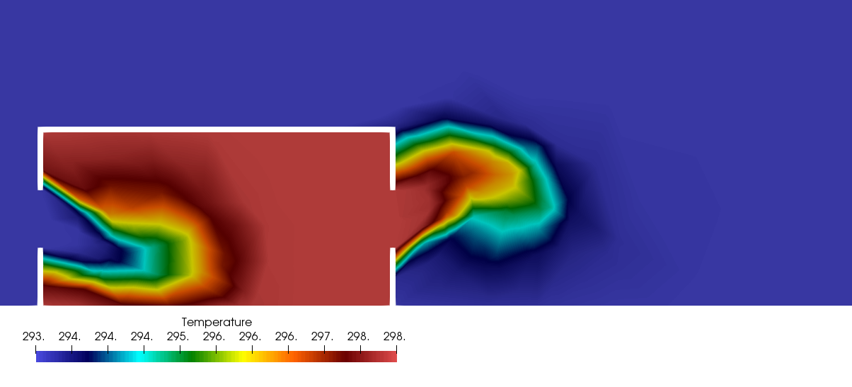
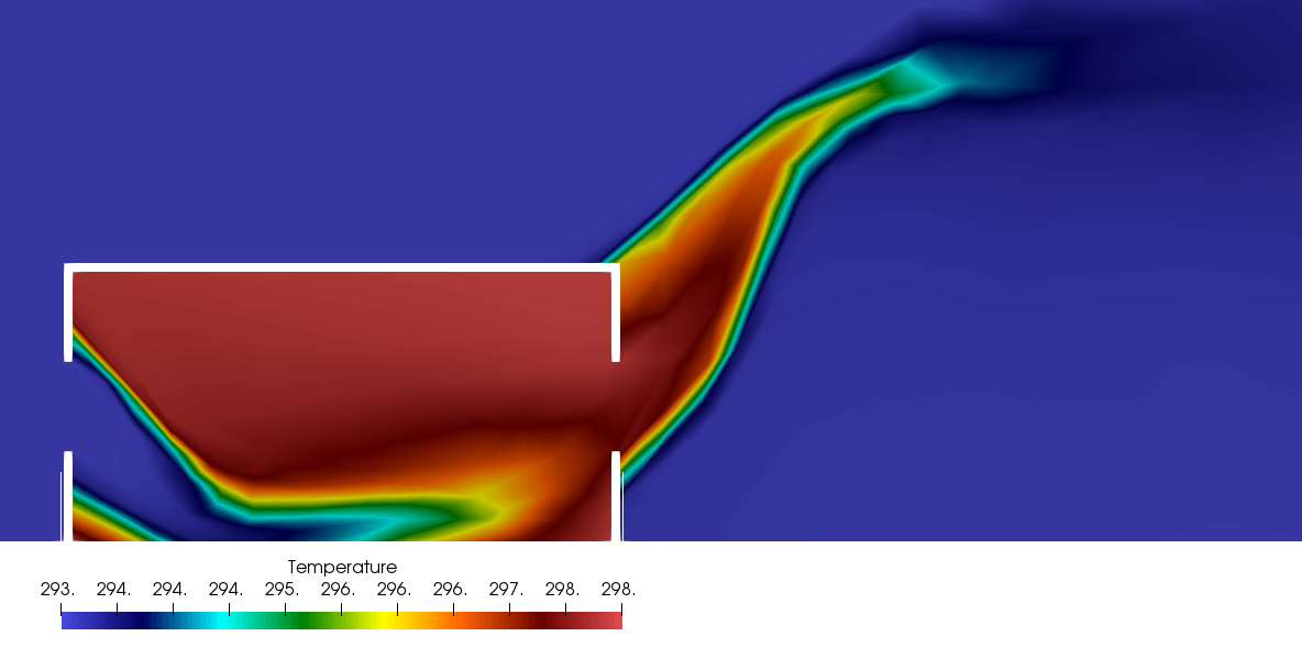
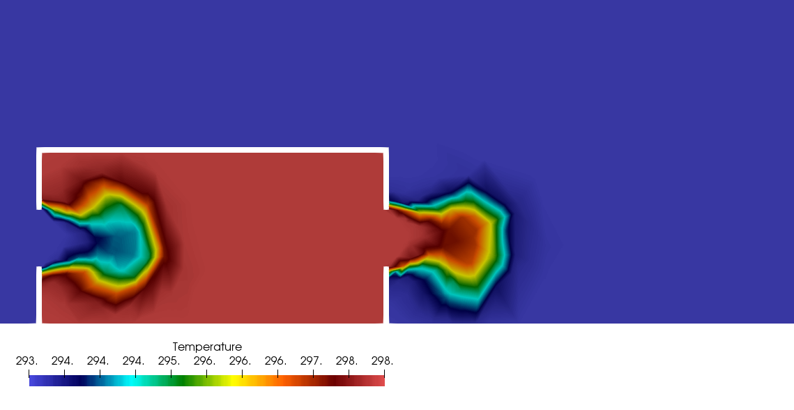
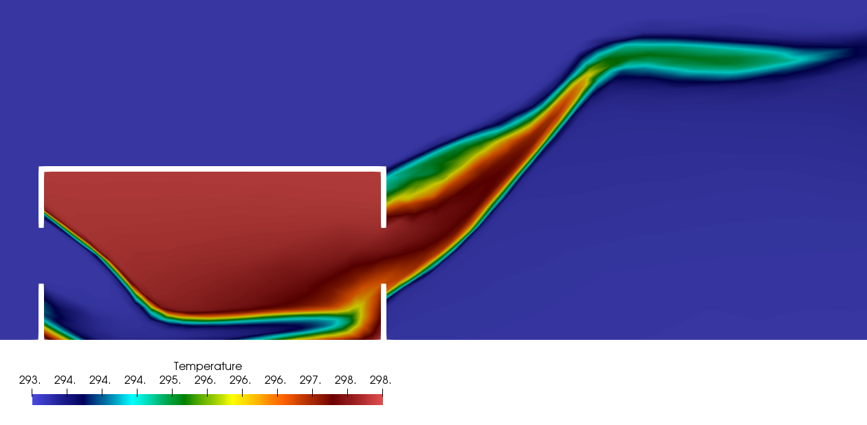
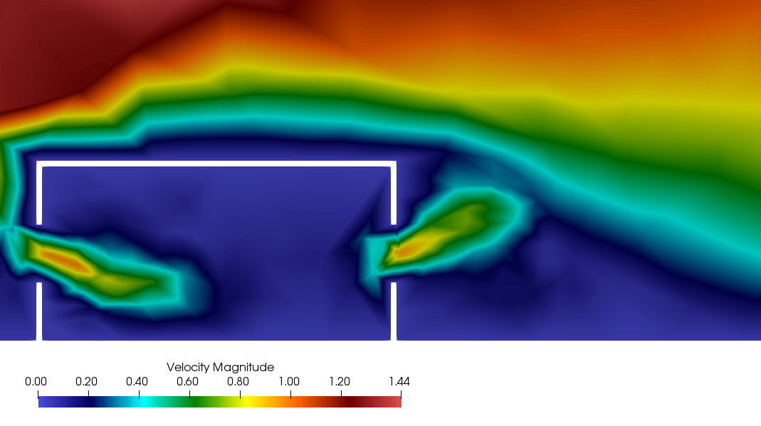
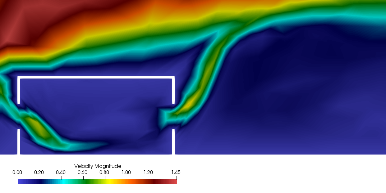
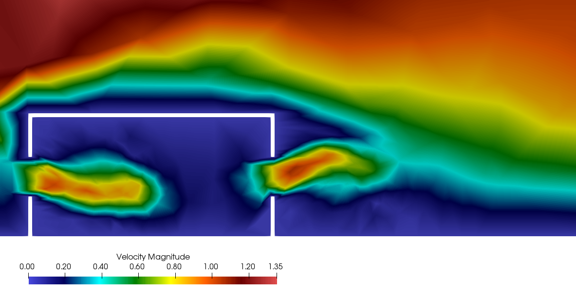
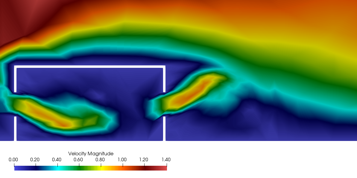
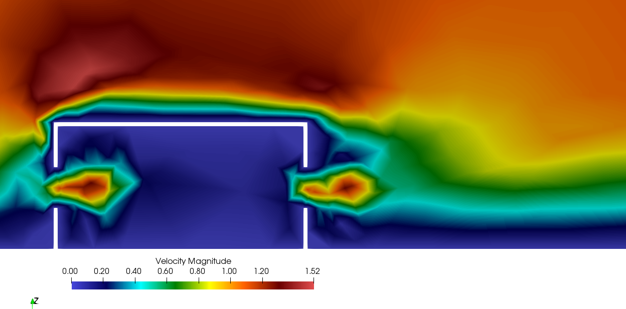
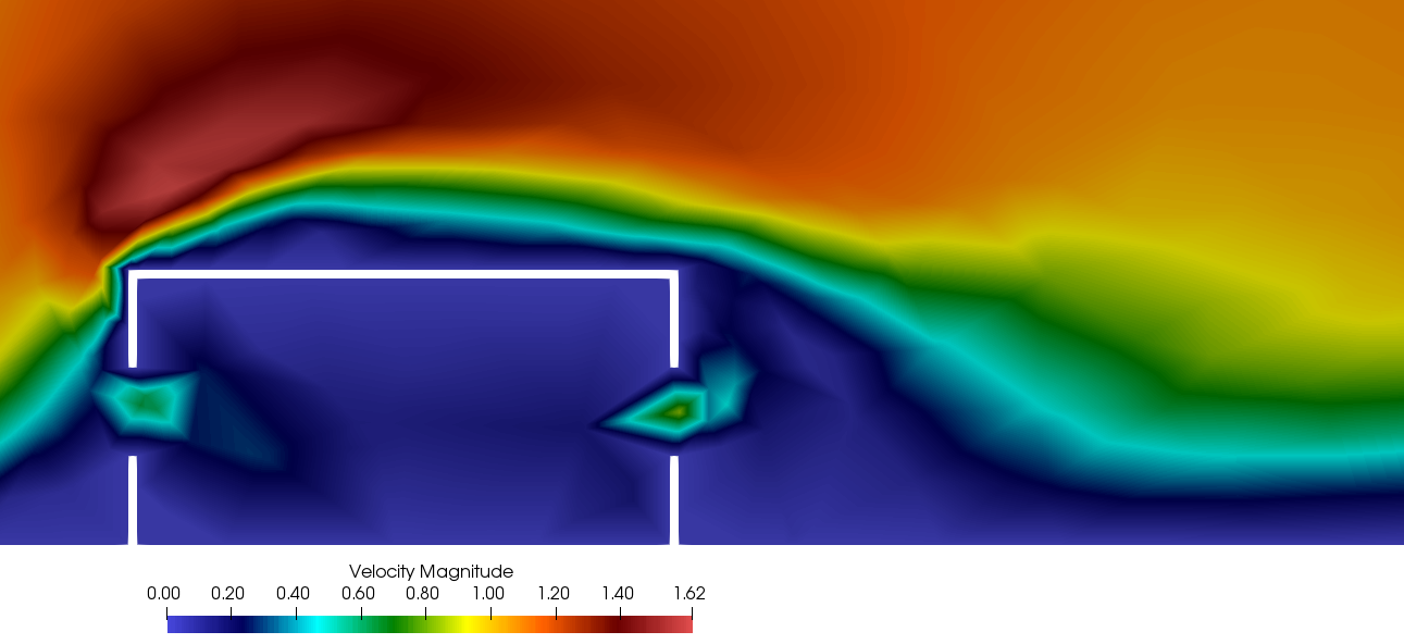
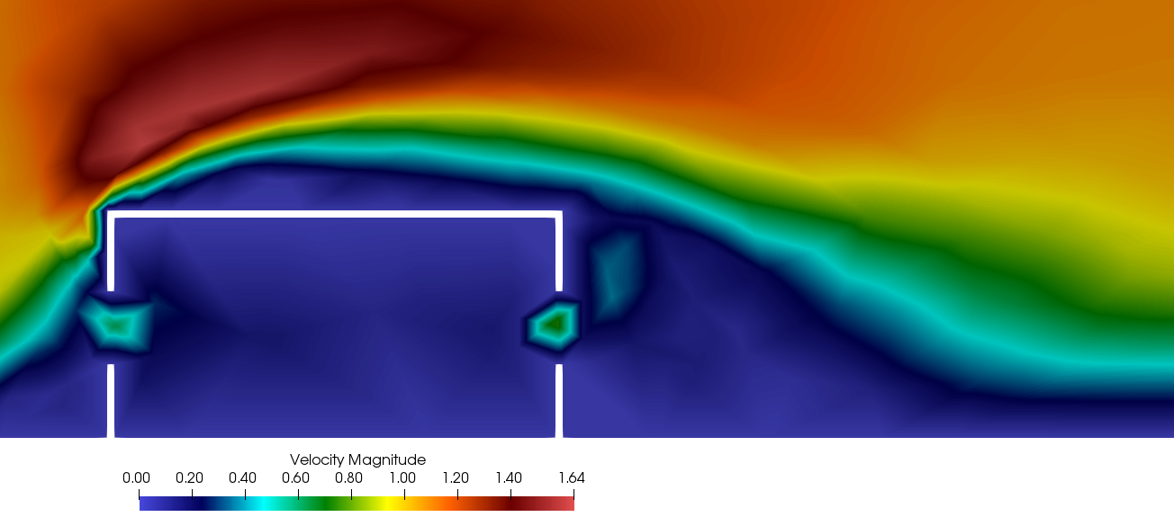
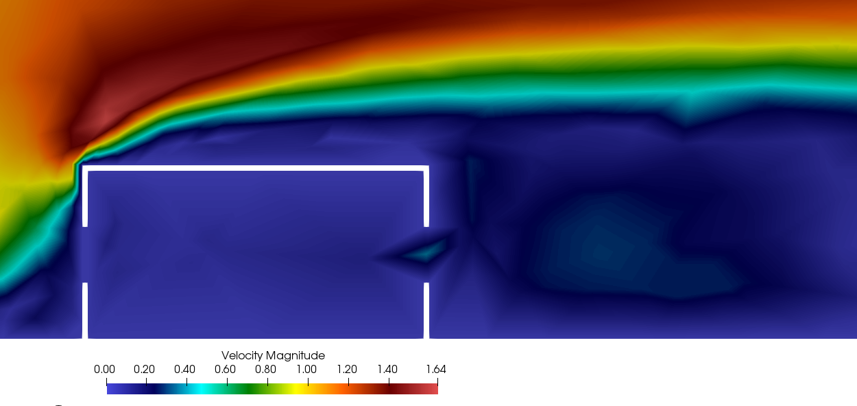
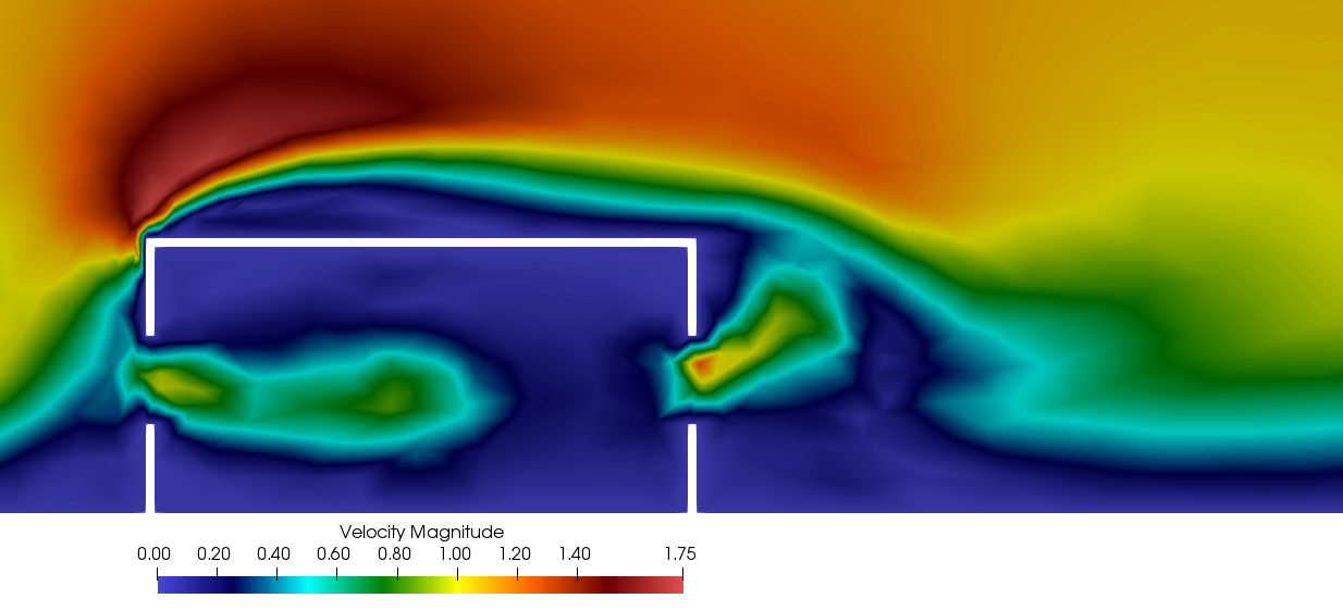
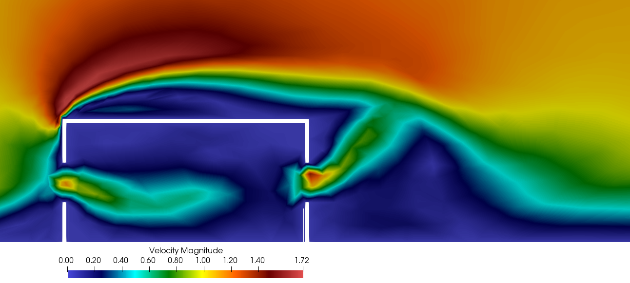
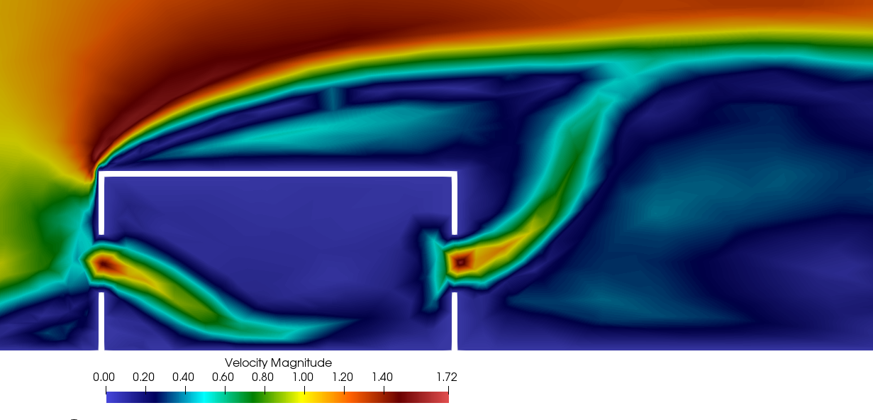
The following examples use a slip boundary condition on solid surfaces and for comparison results are shown in Figure 4.17, Figure 4.18 and Figure 4.19.
- •
-
•
Examples 3dBox_Case13g.flml and 3dBox_Case13h.flml prescribe a slip boundary condition applied weakly using the option align_bc_with_cartesian and align_bc_with_surface, respectively.
-
While 3dBox_Case13g.flml runs like a charm (Figure 4.17(b), Figure 4.18(b) and Figure 4.19(b)), example 3dBox_Case13h.flml gives weird results (Figure 4.17(c), Figure 4.18(c) and Figure 4.19(c)) and finally crashes. Indeed, the option align_bc_with_surface, when a slip boundary condition is weakly applied, does not work in Fluidity and the user should instead use the no_normal_flow option.
-
- •


In summary
In summary:
-
•
The option align_bc_with_cartesian should always be preferred if possible.
-
•
Only one no-slip Dirichlet align_bc_with_surface applied strongly is allowed, while several can be used when applied weakly.
-
•
For a slip boundary condition weakly applied, align_bc_with_cartesian type for simple geometry or no_normal_flow type for any geometry should be used. The Dirichlet align_bc_with_surface type does not work.
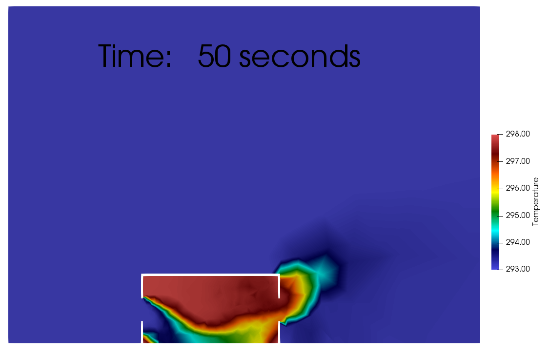
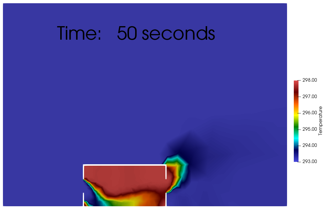
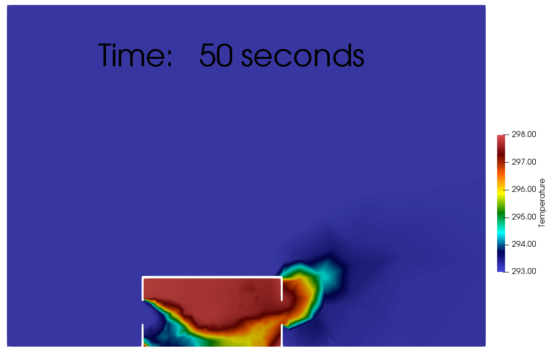
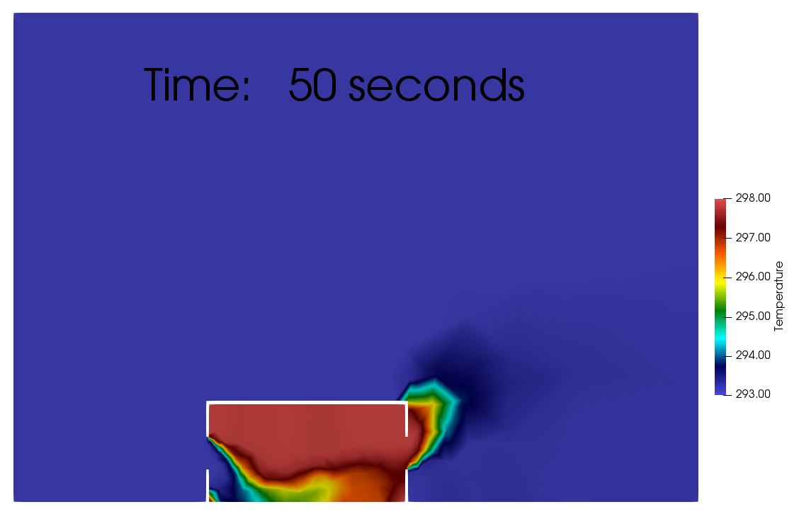
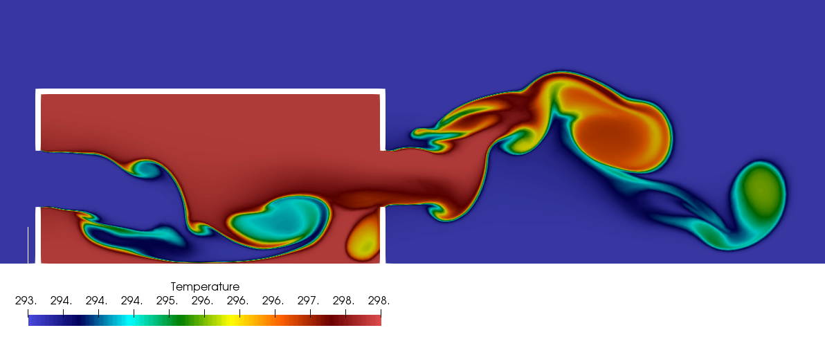
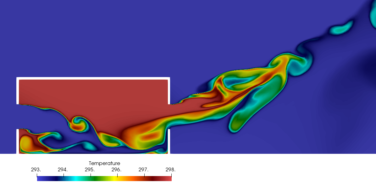
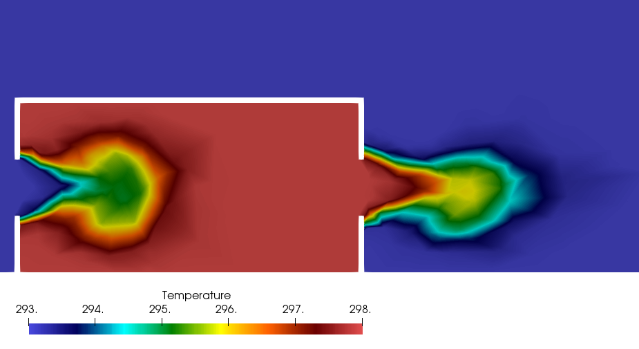
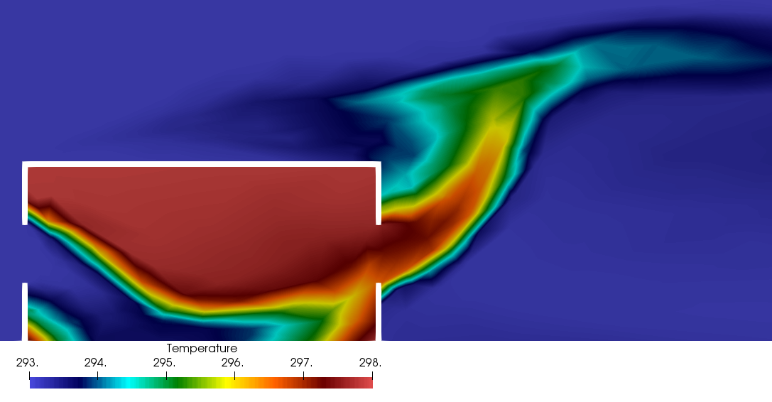
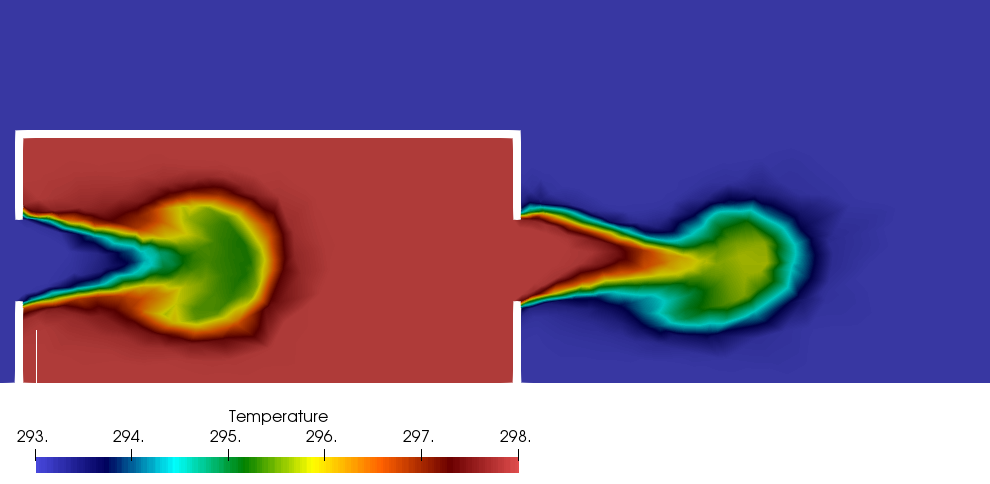
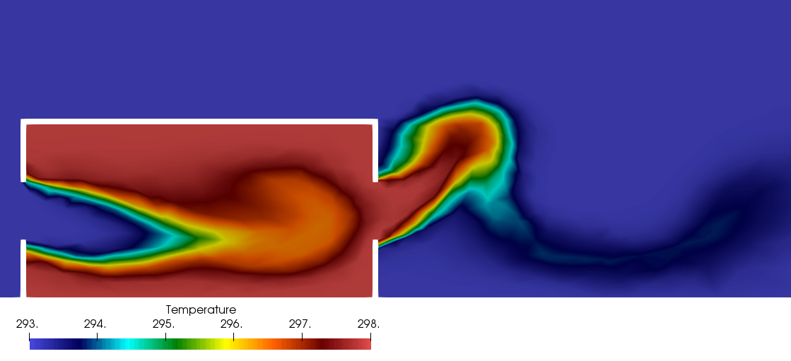
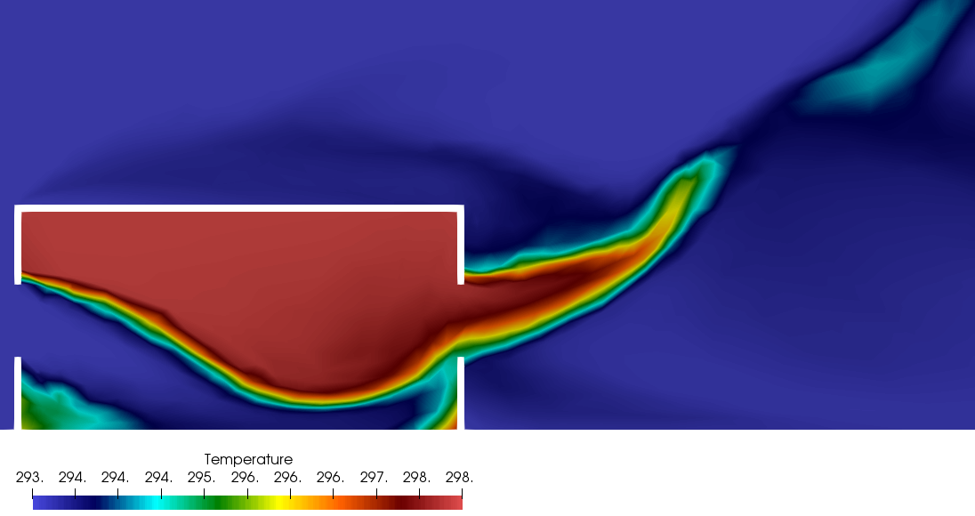
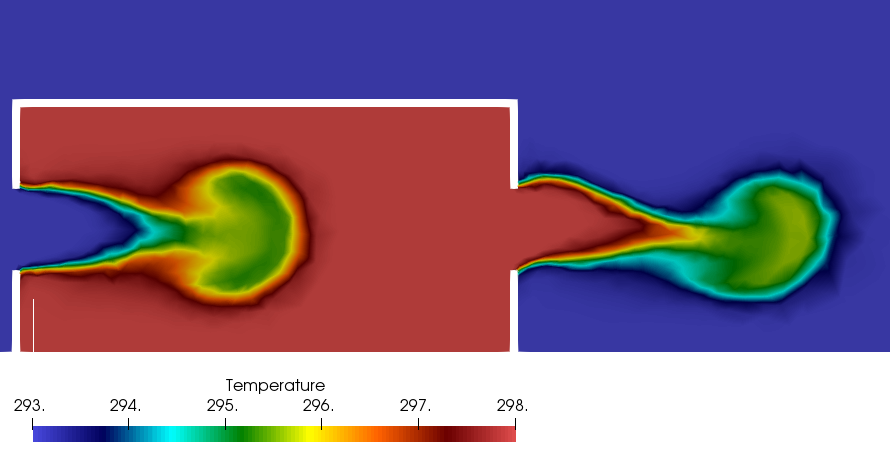
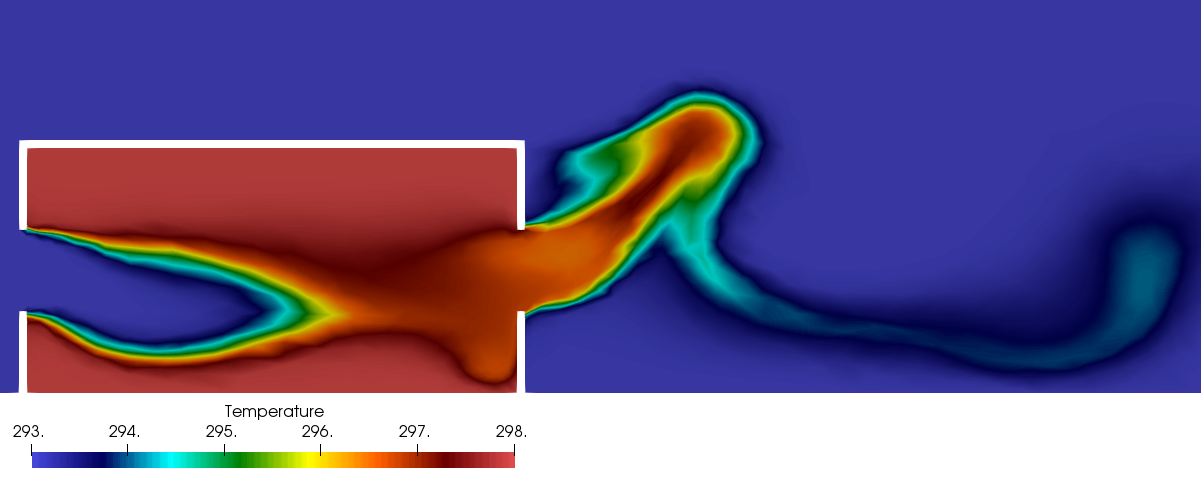
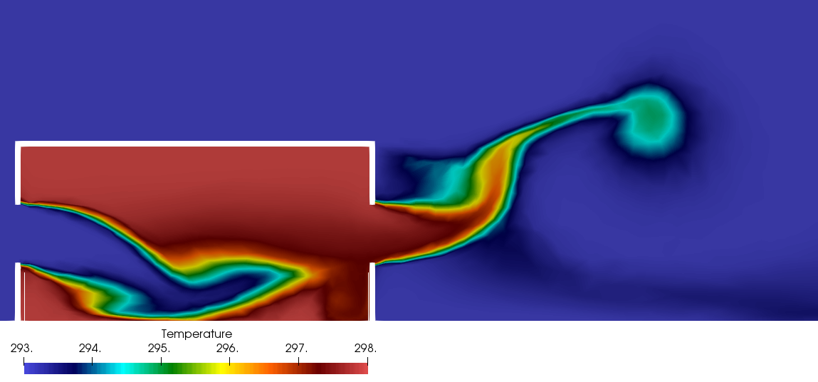
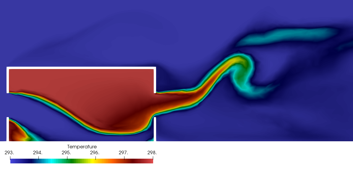
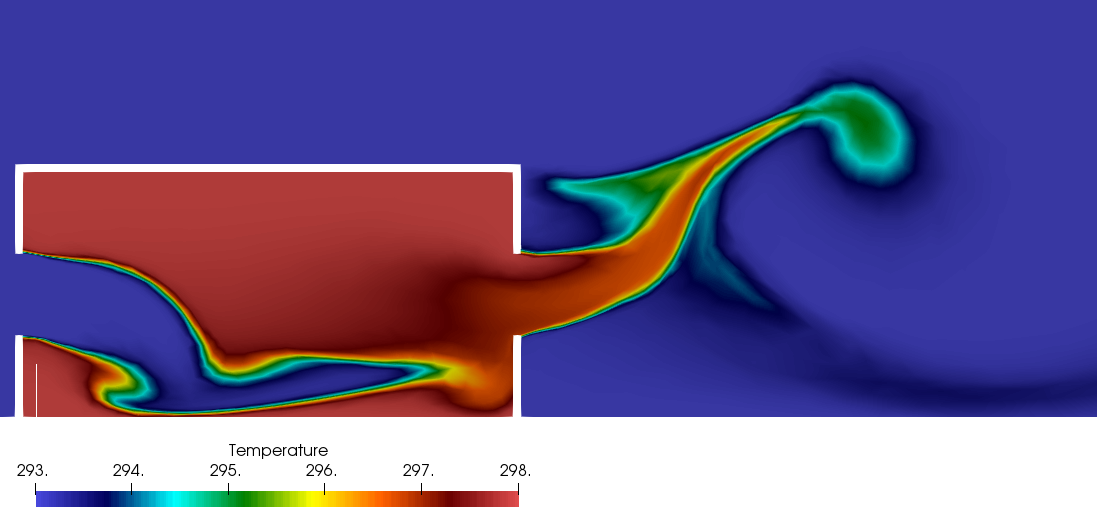
Finally, when defining the velocity boundary conditions at a wall, it is recommended to use a slip boundary condition (normal component only equal to 0) instead of a no-slip condition (all components are set to 0 at the wall) if the boundary layer is not going to be fully resolved with the chosen mesh. Using a no-slip condition can notably be problematic near a heat source and will generate wide variations in the expected temperature. The temperature fields obtained from examples 3dBox_Case4.flml, 3dBox_Case13c.flml, 3dBox_Case13f.flml and 3dBox_Case13g.flml are shown in Figure 4.20. One can noticed that the temperature stays hot in the lower corners of the box when a no-slip strongly applied boundary condition is used, while this hot spots disappear when a slip boundary condition is used or when the boundary condition is applied weakly (which is basically more or less the same…).

4.6 Reference pressure
In every simulations, a reference pressure needs to be given. In Fluidity, there are three different ways to assign the reference pressure:
- •
-
•
The reference pressure is given as a boundary_conditions using a Dirichlet type, usually imposed equal to 0 at the outlet surface (Figure 4.21(c)).
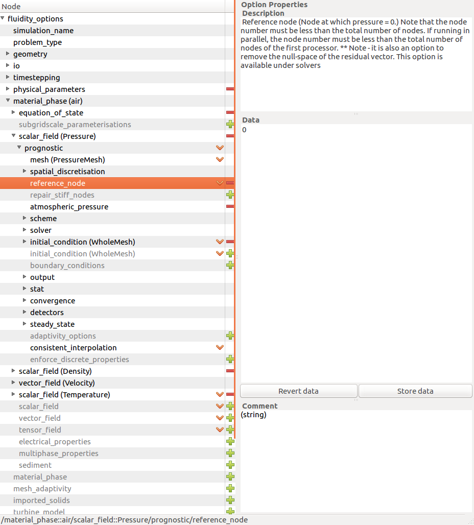
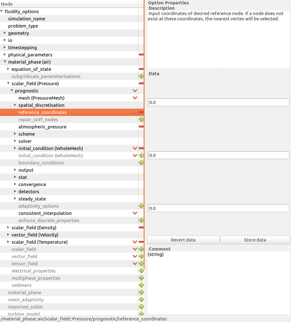
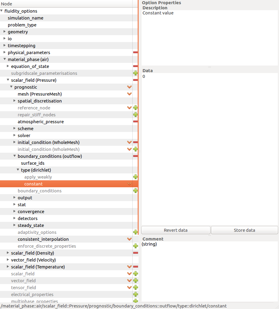
The last option (reference pressure given as a boundary condition) is recommended.
4.7 Common errors
If the simulation crashes, the user can have a look at the file fluidity-err.0, which will give information about the reasons for the crash. Usually, the main and recurrent errors are:
-
•
Mesh errors: The mesh is not consistent and this might be caused by the user not following the steps in Chapter 2.
-
•
Python script errors: The Python language is sensitive to indentation. As such the indentation needs to be checked in the python scripts.
-
•
Non-convergence of the solver: This is frequently caused by the time step being too large. The user should reduce the time step and/or the CFL number.
See also section 8.4 for other tricks.
Chapter 5 Mesh adaptivity
5.1 Explanation and tricks
5.1.1 Explanations
One of the key aspects of Fluidity is its mesh adaptivity capability with unstructured meshes, making it a unique tool that enhances and provides detailed and accurate information at high resolutions within the computational domain. The aim of this section is not to describe the theory behind mesh adaptivity but to explain, from a user point of view, how to set up mesh adaptivity options. The user can refer to [1] and [3] for more details regarding the theory. Different mesh adaptivity algorithms exist and the one used in this document is the hr-adaptivity one based on the change of the connectivity of the mesh and the relocation of the vertices of the mesh while retaining that same connectivity, as described in [3].
The mesh adaptivity process refines automatically the mesh in regions where significant physical processes are happening, which implies that the mesh adaptivity process is field-specific. The mandatory options that need to be turned on for mesh adaptivity are the following:
-
•
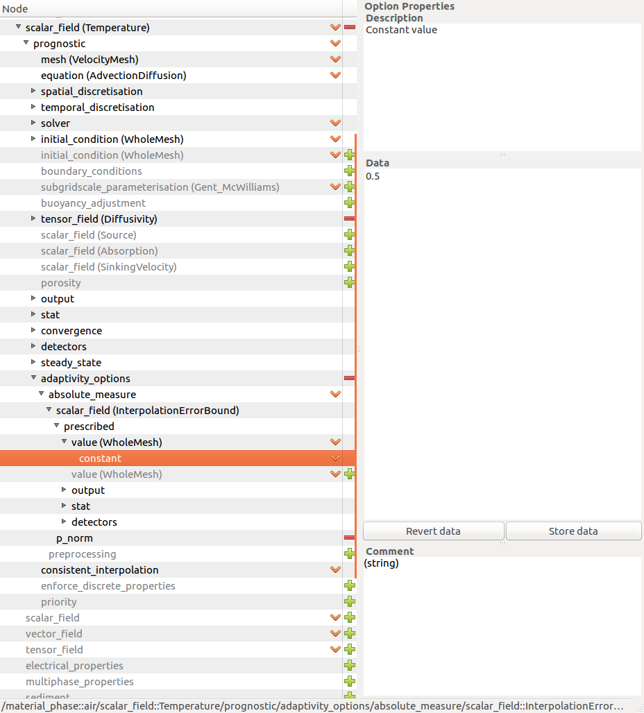
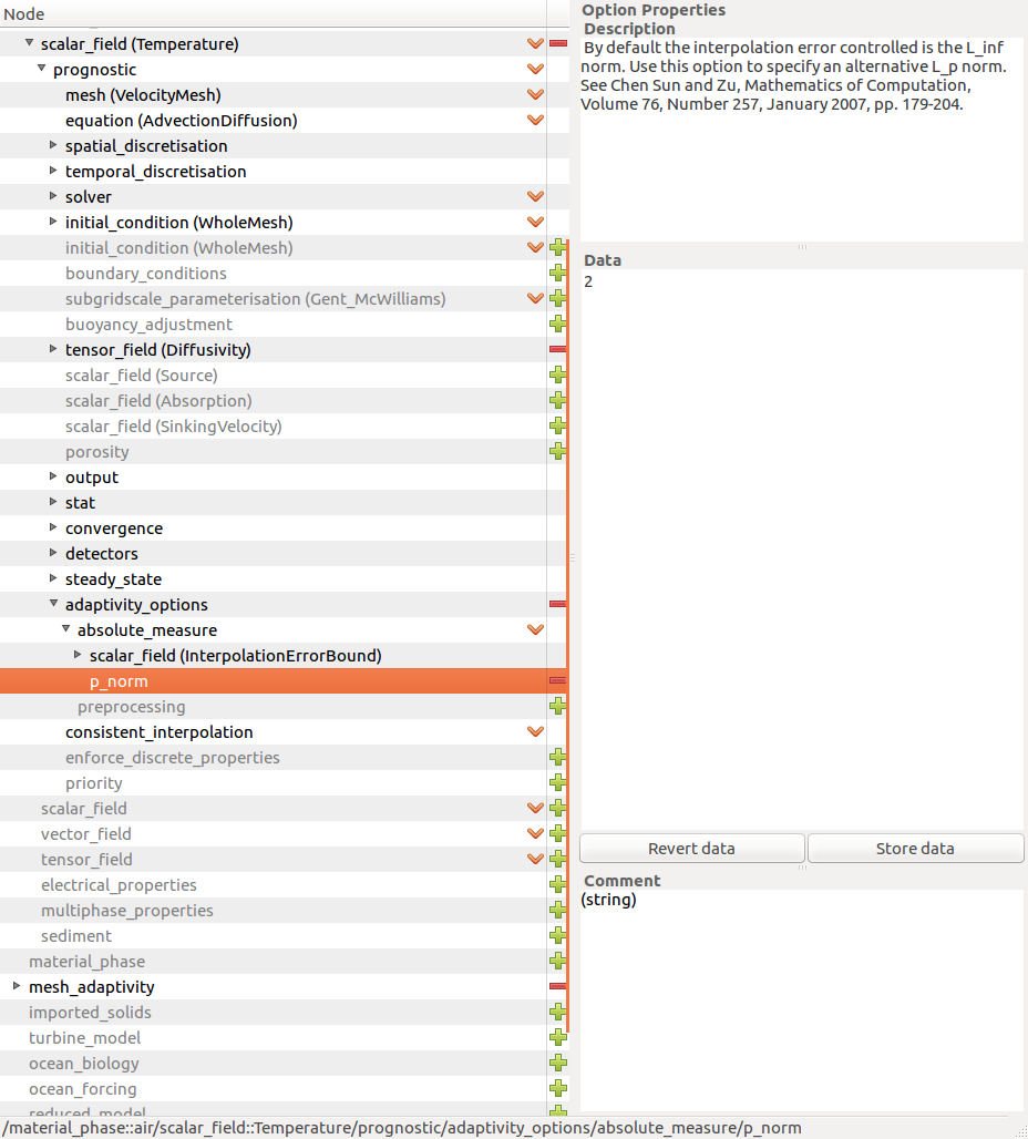
In the Field of interest: As the mesh adaptivity is field-specific, the option adaptivity_options in the field of interest needs to be turned on as shown in Figure 5.1(a) and the error_bound_interpolation value has to be set (see Section 5.1.2). Moreover, the option p_norm can also be enabled and set to 2. Historically, the interpolation error was first controlled in the L∞ norm. The metric formulation which controls the L∞ norm is the simplest, and remains the default in Fluidity (option p_norm is turned off by default). However the L∞ norm can have a tendency to focus the resolution entirely on the dynamics with the largest magnitude. Therefore, the Lp norm, which also includes the influence of the dynamics with smaller magnitudes, can be used. Empirical experience indicates that choosing , and hence the L2 norm, generally gives better results. For that reason we recommend it as default for all adaptivity configurations (Figure 5.1(b)). However, this option can also tend to focus excessively the resolution on dynamics of very small magnitudes. The user should do a prior sensibility analysis to figure out which option is more appropriate for the case considered. See sections 7.5.1 and 7.5.2 of the Fluidity manual [1] for more details.
-
•
In the Mesh_adaptivity options:
-
–
Period: defines how often the mesh should be adapted. This can be set in number of simulation seconds period, or in number of time steps period_in_timesteps. Note that mesh adaptivity has a certain computational cost and a trade-off has to be found between how often the mesh is adapted and the total simulation time. It is recommended that adaptation happens every 10-20 time steps.
-
–
Maximum number of nodes: sets the maximum possible number of nodes maximum_number_of_nodes in the domain (see Section 5.1.2 to know how). In parallel, by default, this is the global maximum number of nodes. If the mesh adaptivity algorithm wants to place more nodes than this, the desired mesh is coarsened everywhere in space until it fits within this limit. In general, the error tolerances should be set so that this is never reached; it should only be a safety catch. If the simulation runs in parallel, make sure that the maximum number of nodes specified is at least nodes.
-
–
Gradation: In numerical simulations, a smooth transition from small elements to large elements is generally important for mesh quality. Therefore, a mesh gradation algorithm is applied to smooth out sudden variations in the mesh sizing function. Various mesh gradation algorithms have been introduced to solve this problem and the one recommended is the anisotropic_gradation, with prescribed on the diagonal and otherwise, as shown in Figure 5.1(c).
-
–
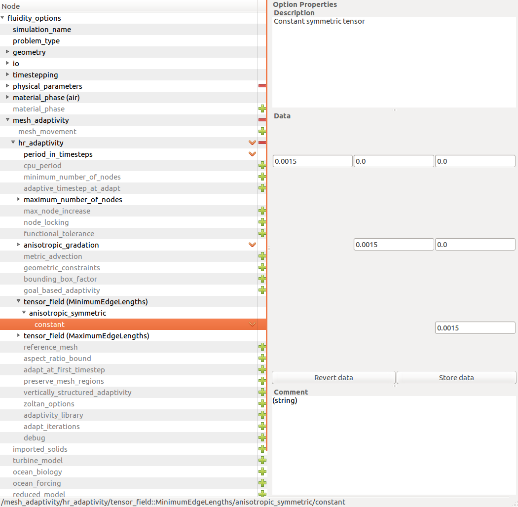
Minimum edge length: is the minimum edge length of an element allowed in the mesh (in meters). The input to this quantity is a tensor allowing one to impose different limits in different directions (see Figure 5.1(d)). See Section 5.1.2 to know how to find the appropriate value. This condition is not a hard constraint and the user may observe the constraint being (slightly) broken in places.
-
–
Maximum edge length: is the maximum edge length of an element allowed in the mesh (in meters). The input to this quantity is a tensor allowing one to impose different limits in different directions. See Section 5.1.2 to know how to find the appropriate value. This condition is not a hard constraint and the user may observe the constraint being (slightly) broken in places.
-
–
The minimum and maximum edge lengths and the maximum number of nodes, in combination with the interpolation error bound, will define how the resolution of the mesh varies with adaptation.

5.1.2 Tricks to set up mesh adaptivity
Setting up the correct parameters needed for mesh adaptivity is not trivial and there are no universal rules. The user needs to experiment with the three main parameters which are: Interpolation_error_bound, Minimum_edge_length and Maximum_edge_length. However, here are some basic rules that can be followed.
-
•
Maximum number of nodes: As a start, the user is suggested to use a relatively small number of maximum nodes to test all the options: between and is recommended. This value can be increased later.
-
•
Minimum edge length: The minimum edge length should be quite large to start with. The value , where is the height of the domain OR the value , where is a characteristic length of your geometry (here, the height of the openings for example), are recommended. This value can be progressively decreased afterwards to reach the resolution needed.
-
•
Maximum edge length: The maximum edge length should be quite large to start with and the value , where is the height of the domain, is recommended.
-
•
Interpolation error bound: The general advice would be to start with a high interpolation error, 10 of the range of the field considered being a good rule of thumb. As this value will certainly be too high, it is then recommended to reduce this value by small increments until reaching a refinement able to represent the desired dynamics. In any case, the interpolation error bound value should be the main parameter to vary to control the resolution of the adapted meshes. The value of p_norm should be equal to as a first try. However, using might also tend to focus the resolution on dynamics of too small magnitudes. The user should do a prior sensibility analysis with and without the p_norm function to figure out which option is more appropriate for the case considered.
Python scripts can be used to vary the specified lengths over the domain, allowing finer resolutions over areas of interest for instance. This will be discussed in Section 5.4.
Important note: The velocity field and/or the temperature (or any scalar field) can be adapted. Several field can be taken into account during adaptation. However, it is not recommended to adapt the pressure field: for cases involving indoor-outdoor exchanges and/or the urban environment, one might even say it is forbidden!
5.2 Summary of the simulations
Table 5.1 summarises the different simulations presented in the next sections.
|
Case
Nbr |
Initial
Test Case Nbr |
Field
adapted |
Interpolation
error bound |
Advected
mesh |
Section |
|---|---|---|---|---|---|
| 6a | 5a | Temperature | 0.5 | No | 5.3.2 |
| 6b | 5a | Temperature | 0.3 | No | 5.3.2 |
| 6c | 5a | Temperature | 0.1 | No | 5.3.2 |
| 6d | 5a | Temperature | 0.05 | No | 5.3.2 |
| 7a | 5a | Velocity | 0.5 | No | 5.3.3 |
| 7b | 5a | Velocity | 0.25 | No | 5.3.3 |
| 7c | 5a | Velocity | 0.15 | No | 5.3.3 |
| 7d | 5a | Velocity | 0.1 | No | 5.3.3 |
| 8 | 5a |
Temperature
Velocity |
0.15
0.15 |
No | 5.3.4 |
| 9 | 2b |
Temperature
Velocity |
075
0.045 |
No | 5.4 |
| 10 | 5a | Temperature | 0.1 | Yes | 5.5 |
5.3 Field specific adaptation
5.3.1 Set-up of examples
Boundary conditions
In examples 3dBox_Case6a.flml to 3dBox_Case7d.flml, the initial velocity and the inlet velocity are set to m/s and the interior of the box is set to 298 K, while the outside remains at ambient temperature 293 K. These examples are similar to example 3dBox_Case5a.flml which is set up without mesh adaptivity, i.e on a fixed mesh.
CFL number
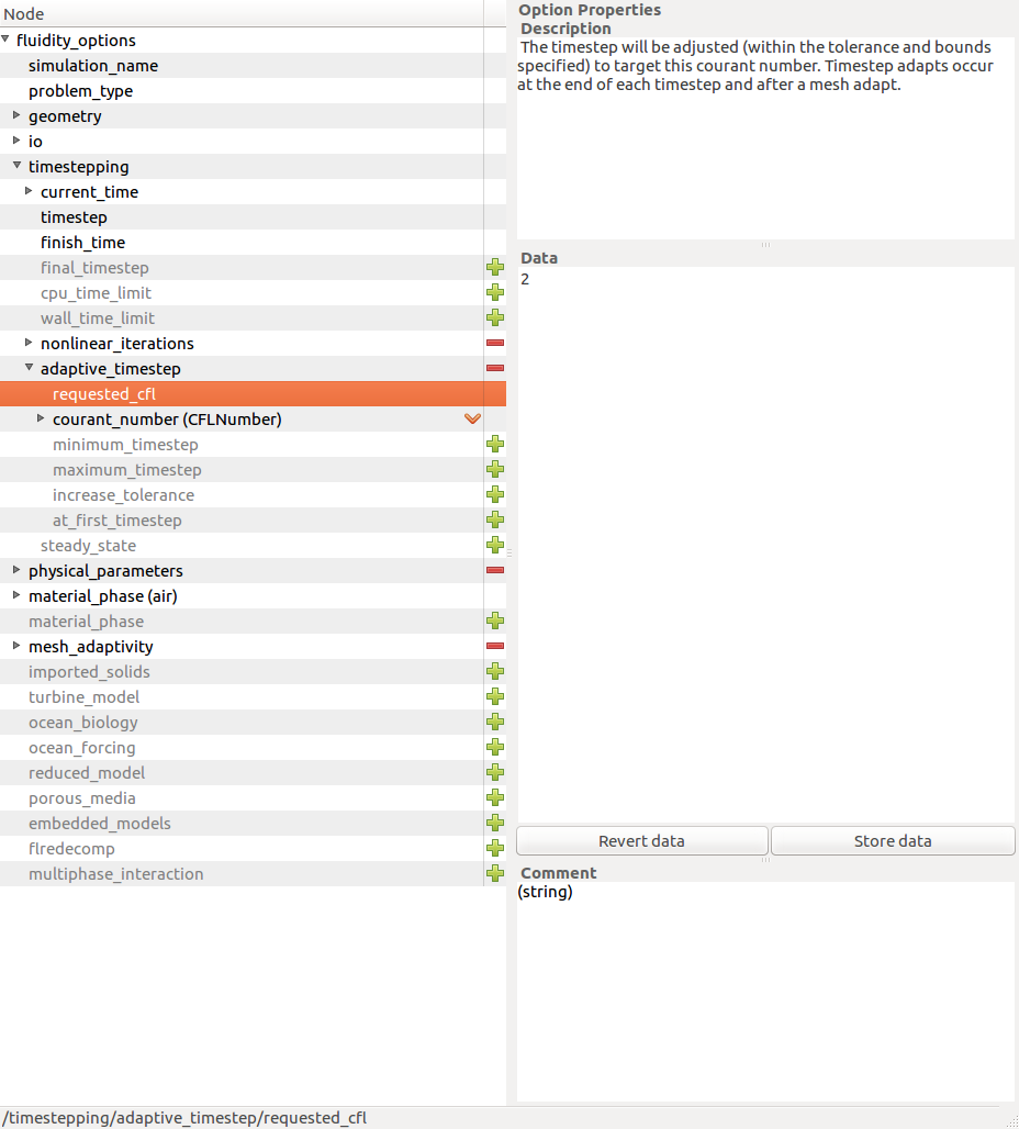
To avoid any crash of the simulations, the time step is now also adaptive using a CFL condition as described in Section 3.2.2 and the CFL number is taken equal to 2 in the following examples (Figure 5.2). This value can be increased later on to speed up the simulations. However, it is recommended to the user to do a sensibility analysis of the results as a function of the CFL number to ensure that important information is not missing.
General mesh adaptivity options
In the following sections, mesh adaptivity will be performed based on the temperature field only (Section 5.3.2), the velocity field only (Section 5.3.3) and both the velocity and temperature fields (Section 5.3.4). When the user wants to adapt several fields, it is recommended firstly to analyse each field independently as done in the following sections.
The maximum number of nodes is set equal to and the mesh is adapted every 10 time steps.
The characteristic length of the domain is taken to be the windows opening, i.e. 1 m: the minimum edge length is set up to , i.e. 0.01 m. The height of the domain is 21 m: the maximum edge length is set up to , i.e 2.1 m.
5.3.2 Adaptation based on the temperature field
In this section, the mesh adaptivity process is prescribed based on the temperature field only.
Mesh adaptivity options
The range of the temperature is between 293 K and 298 K, i.e. a difference of 5 K. The error_bound_interpolation is in a first run set up at 10 of this temperature range: the value is used in example 3dBox_Case6a.flml. Then the error_bound_interpolation is progressively decreased to values equal to 0.3 (6 of the temperature range) in 3dBox_Case6b.flml, 0.1 (2 of the temperature range) in 3dBox_Case6c.flml and 0.05 (1 of the temperature range) in 3dBox_Case6d.flml.
These examples can be run using the commands:
Results and discussion
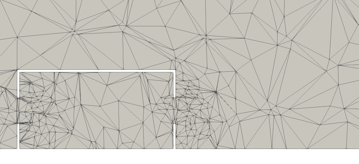
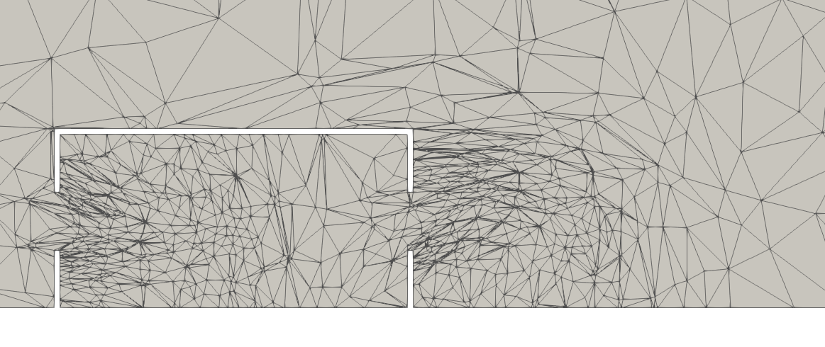
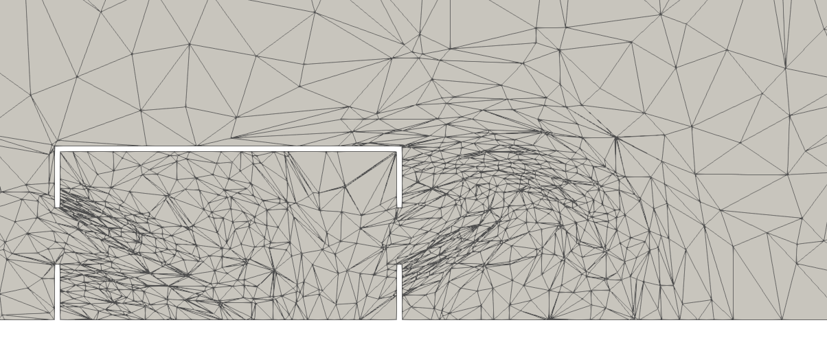
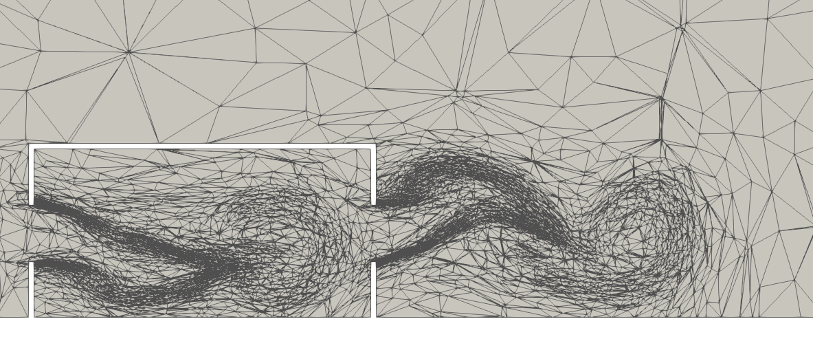
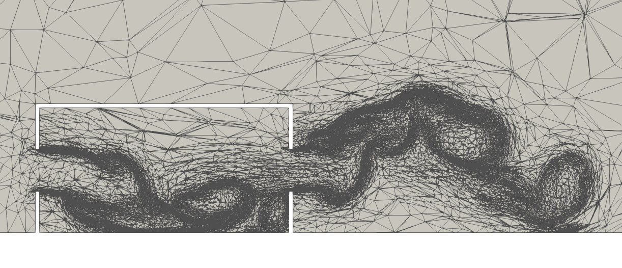
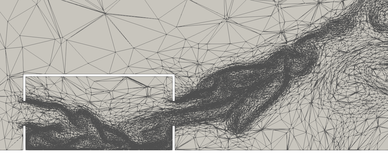
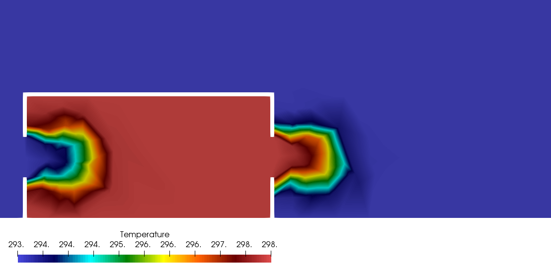
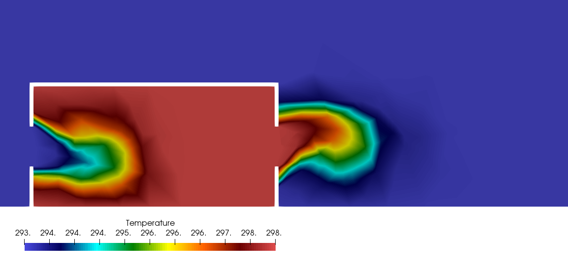
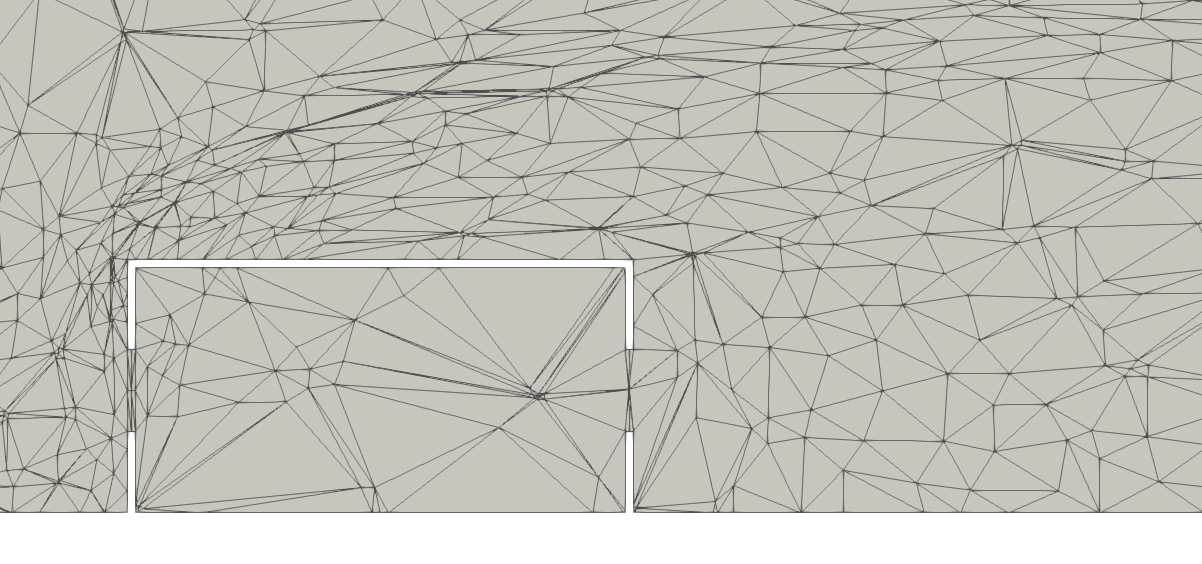
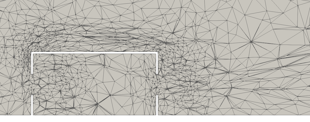
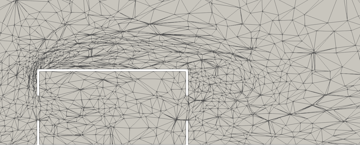
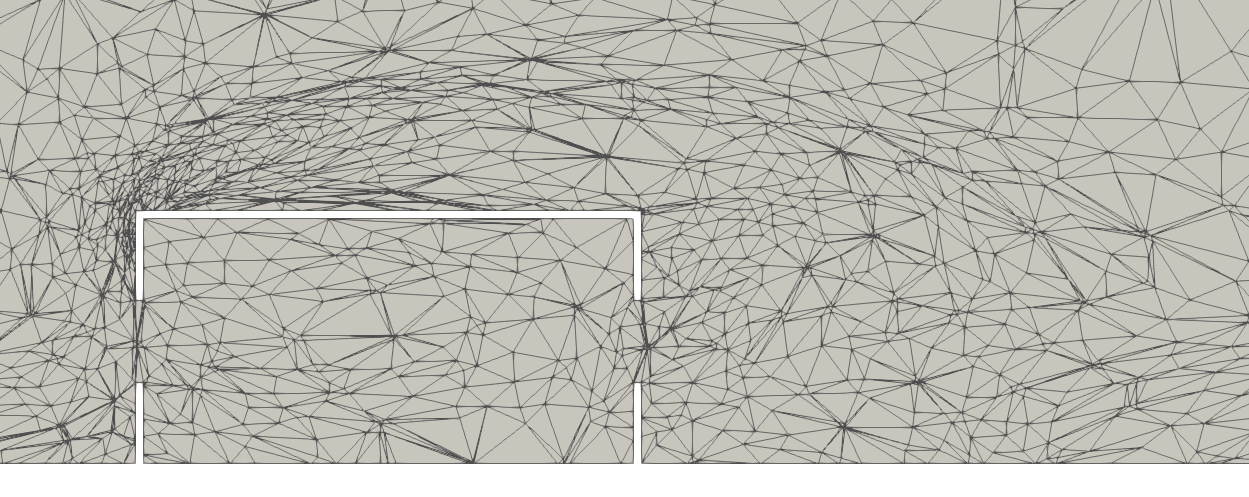
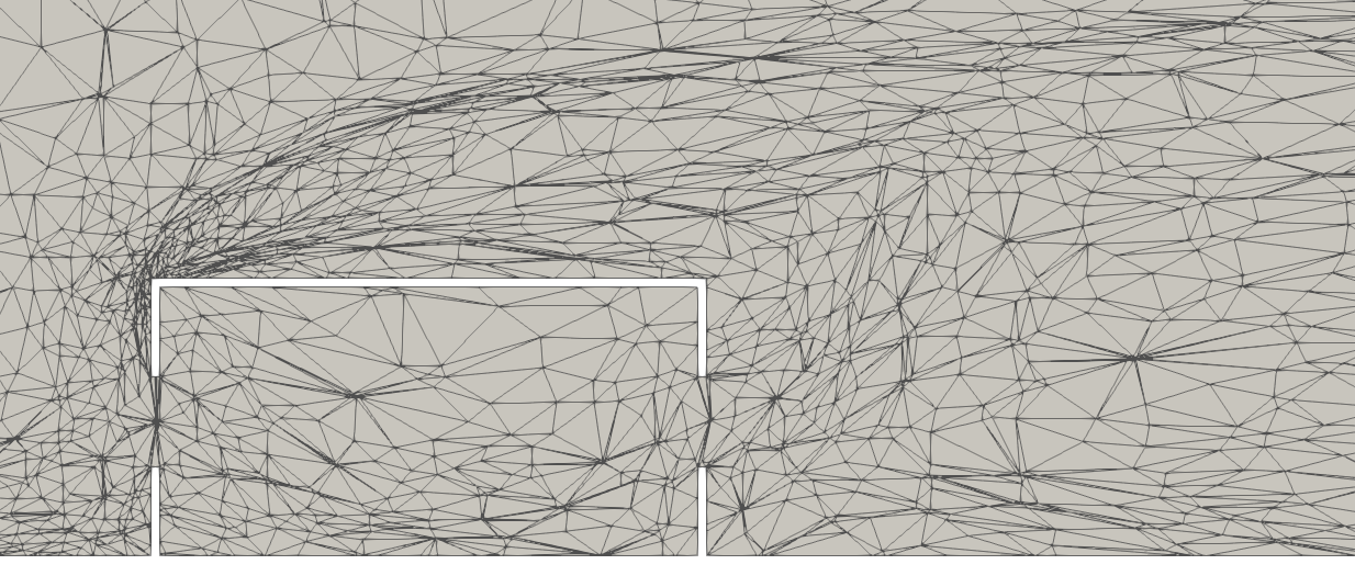
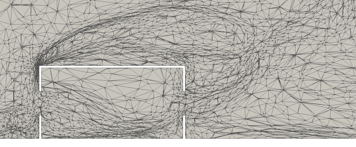
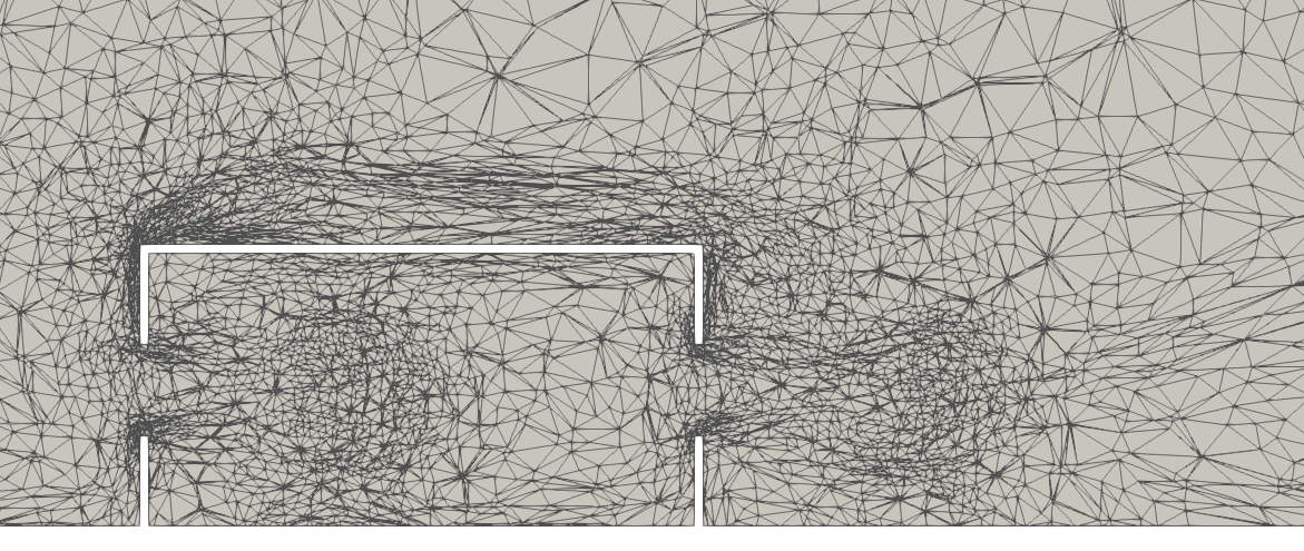
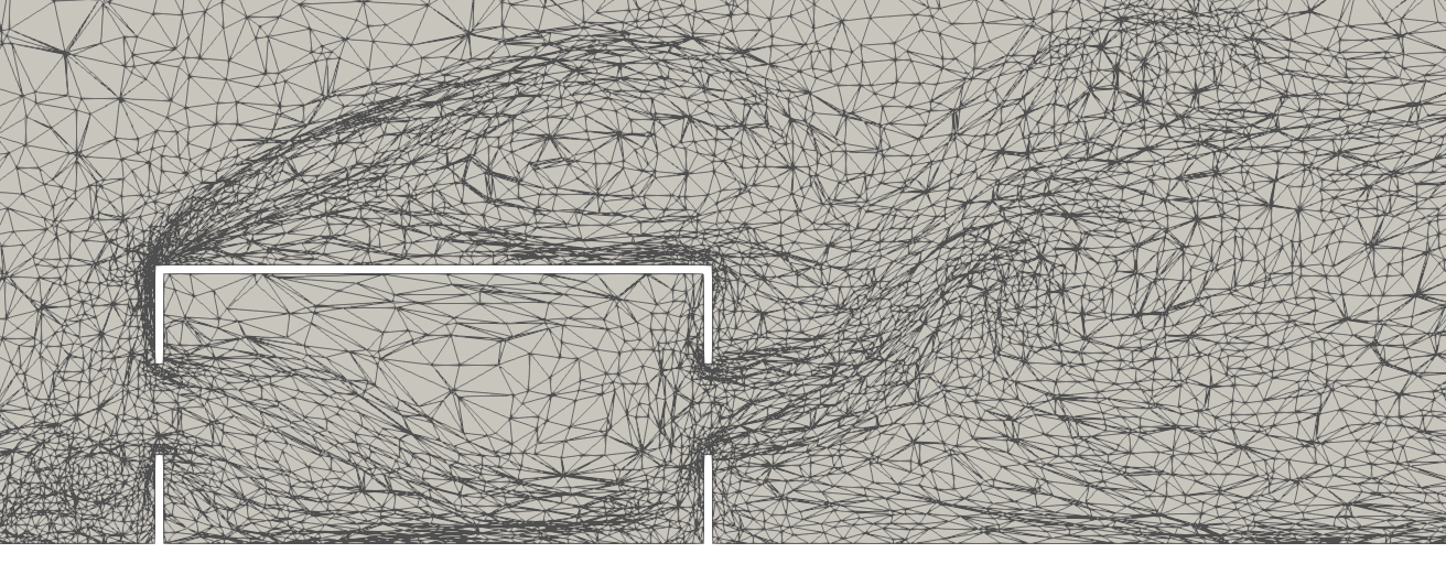
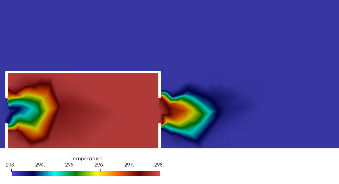
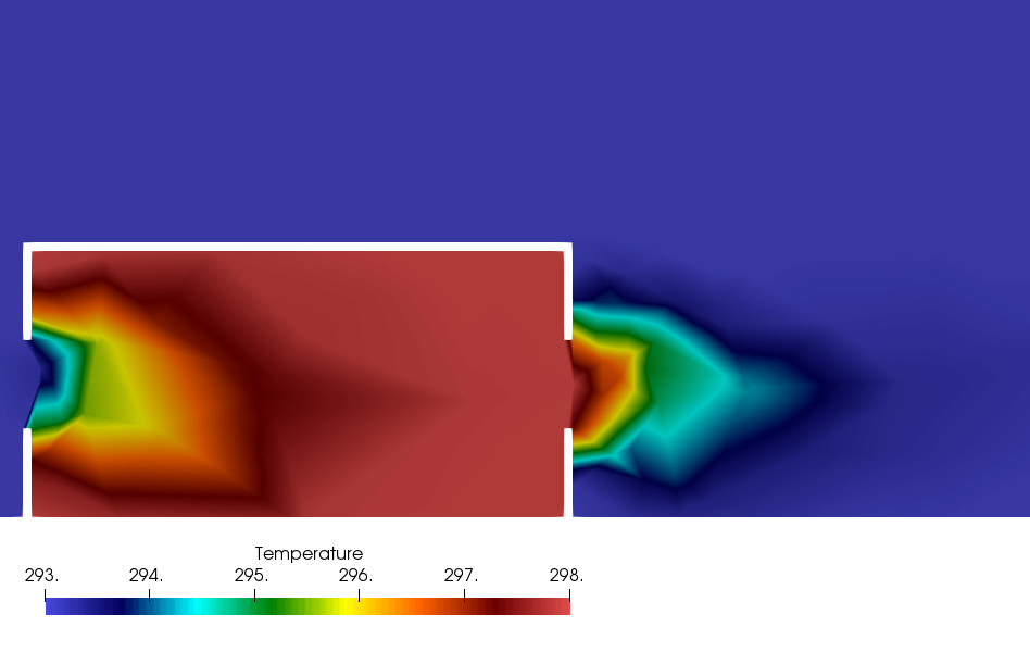
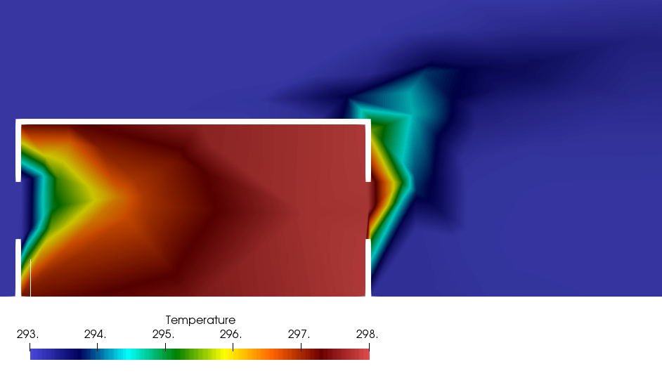
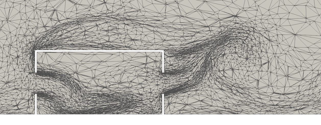
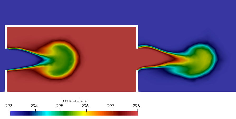
Snapshots of the meshes are shown in Figure 5.3, Figure 5.4, Figure 5.5 and Figure 5.6. Snapshots of the temperature field are shown in Figure 5.7, Figure 5.8, Figure 5.9 and Figure 5.10. Snapshots of the velocity field are shown in Figure 5.11, Figure 5.12, Figure 5.13 and Figure 5.14. Go to Chapter 10 to learn how to visualise the results using ParaView.
For a given error_bound_interpolation, as shown in Figure 5.3, Figure 5.4, Figure 5.5 and Figure 5.6 the mesh is adapting based on the temperature field, i.e. mainly within the box and at the outlet of the box. Indeed, decreasing the value of the error_bound_interpolation results in finer mesh in those regions. However, it is important to mention that the computational time is by consequence larger, see Section 5.3.5. Choosing an error_bound_interpolation higher to 0.3 seems to lead to poor mesh quality (in that particular case). Even with small error_bound_ interpolation and if the temperature field is well resolved, the velocity field is not properly captured due to a poor mesh quality, especially around the box.


5.3.3 Adaptation based on the velocity field
In this section, the mesh adaptivity process is prescribed based on the velocity field only.
Mesh adaptivity options
Even if the initial inlet velocity is prescribed equal to 1 m/s, it is not recommended to use 1 m/s as the upper bound to determine the error_bound_interpolation. Indeed, the velocity magnitude in the domain will probably be higher than this value and estimate the error_bound_interpolation based on 1 m/s will lead to a too small value as a first guess. Therefore, based on the run performed in examples 3dBox_Case6*.flml, the velocity range seems to be between 0 m/s and approximately 5 m/s, i.e. a difference of 5 m/s. The error_bound_interpolation is, in a first run, set up at 10 of this velocity range: the value is used in example 3dBox_Case7a.flml. Then the error_bound_interpolation is progressively decreased to values equal to 0.25 (5 of the velocity range) in 3dBox_Case7b.flml, 0.15 (3 of the velocity range) in 3dBox_Case7c.flml and 0.1 (2 of the velocity range) in 3dBox_Case7d.flml.
These examples can be run using the commands:
Results and discussion
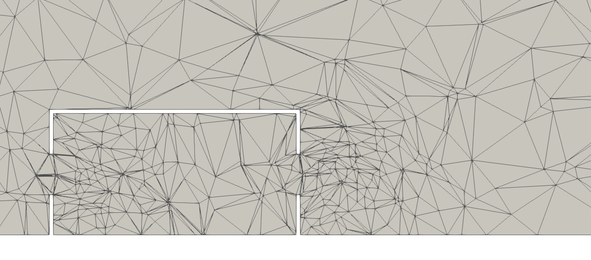
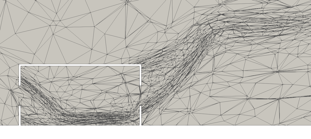
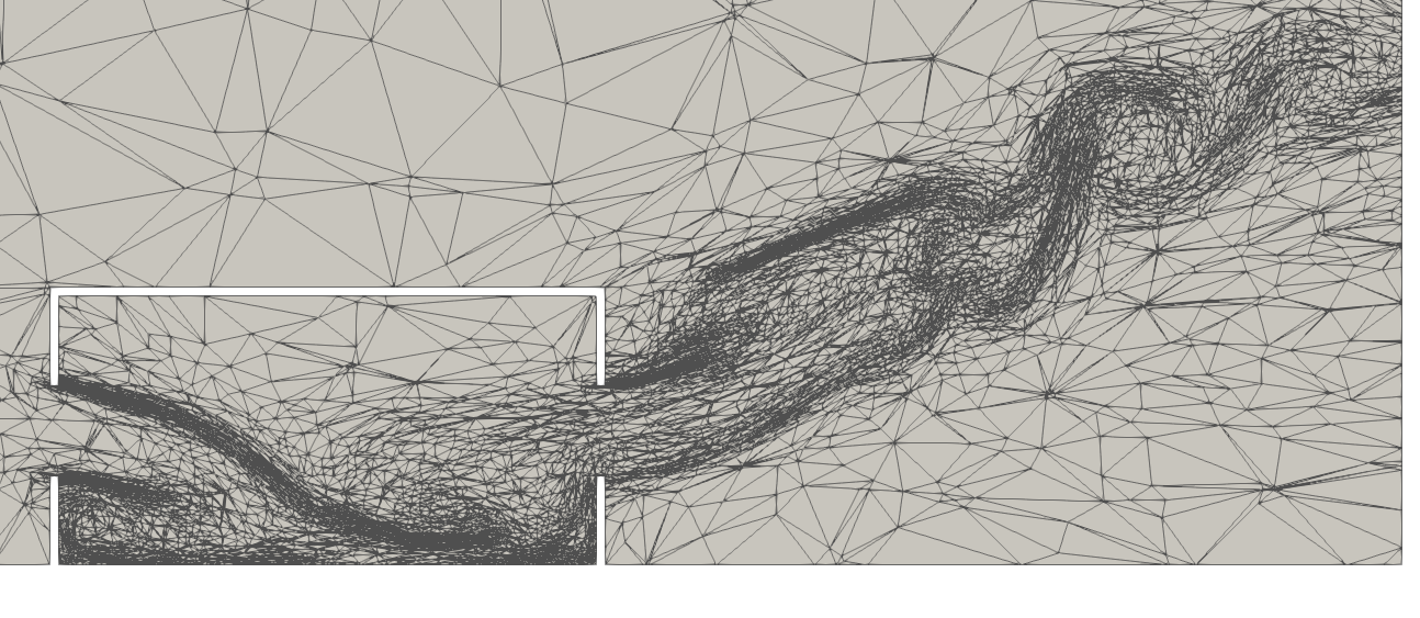
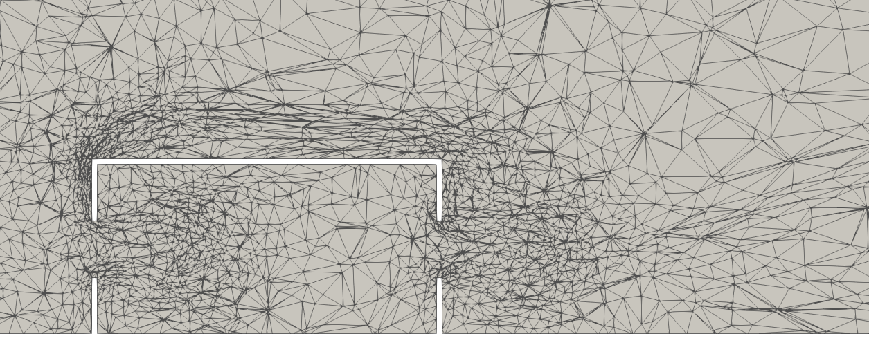
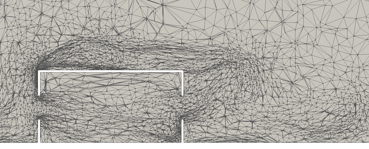
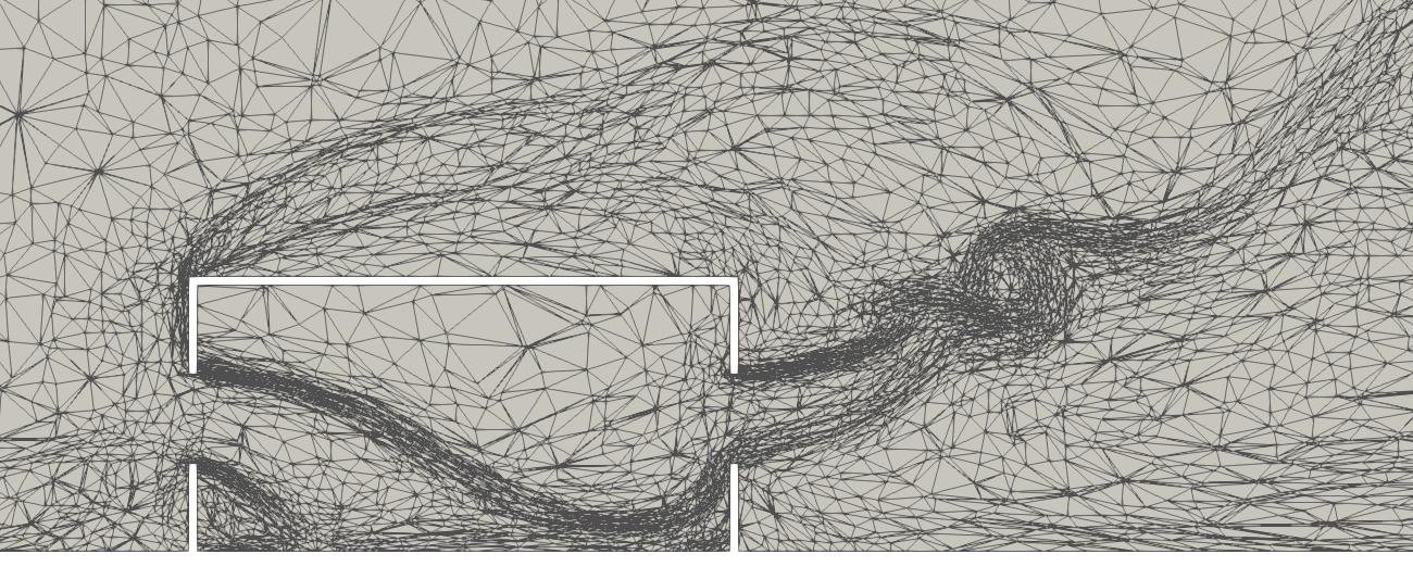
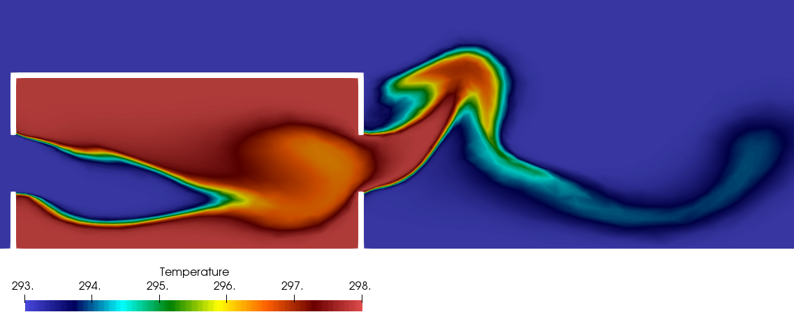
Snapshots of the meshes are shown in Figure 5.15, Figure 5.16, Figure 5.17 and Figure 5.18. Snapshots of the temperature field are shown in Figure 5.19, Figure 5.20, Figure 5.21 and Figure 5.22. Snapshots of the velocity field are shown in Figure 5.23, Figure 5.24, Figure 5.25 and Figure 5.26. Go to Chapter 10 to learn how to visualise the results using ParaView.
For a given error_bound_interpolation, as shown in Figure 5.15, Figure 5.16, Figure 5.17 and Figure 5.18 the mesh is adapting based on the velocity field, i.e. mainly at the openings and around the exterior surfaces of the box. Indeed, decreasing the value of the error_bound_interpolation results in finer mesh in those regions. Choosing an error_bound_interpolation higher to 0.15 seems to lead to poor mesh quality (in that particular case). Even with small error_bound_interpolation and if the velocity field is well resolved, the temperature field is not properly captured due to a poor mesh quality, especially within the box.


5.3.4 Adaptation based on the velocity and the temperature fields
In this section, the mesh adaptivity process is prescribed based on both the velocity field and the temperature field.
Mesh adaptivity options
Based on the run performed in examples 3dBox_Case6*.flml and 3dBox_Case7*.flml, the error_bound_interpolation values for the temperature and the velocity are chosen to be both equal to 0.15 in example 3dBox_Case8.flml. Note that using the same value is a coincidence, and these values can be of course different. These values were chosen to capture properly both the temperature and the velocity fields, while keeping an acceptable computational time for the purpose of this manual. It is therefore recommended to use 0.1 for both field to fully capture the dynamics.
This example can be run using the command:
Results and discussion
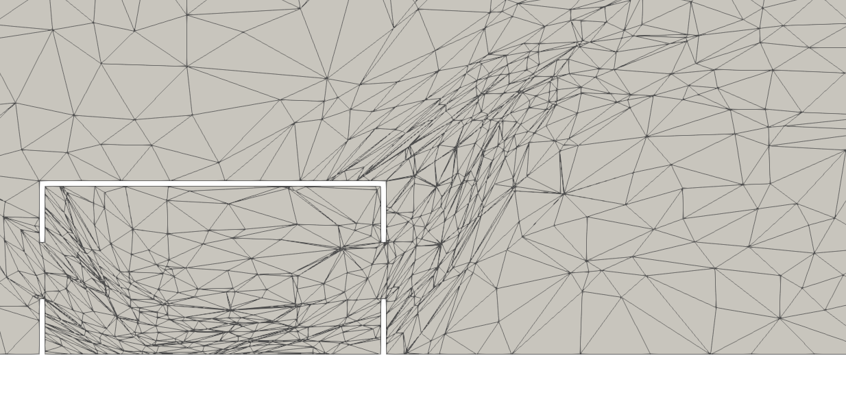
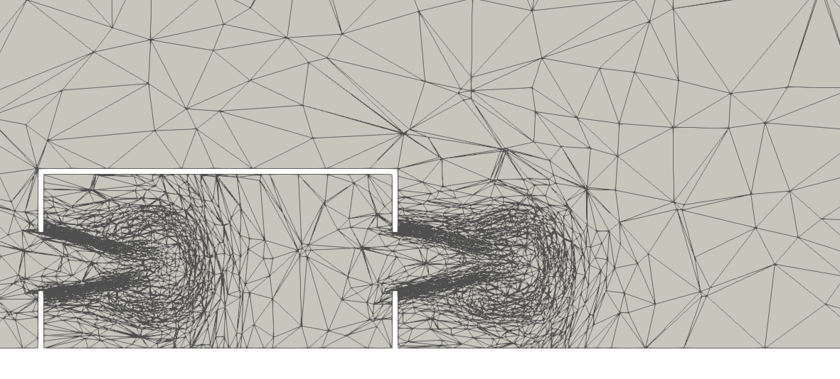
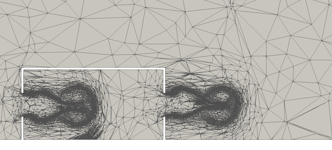
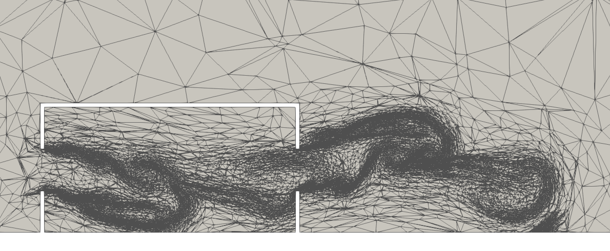
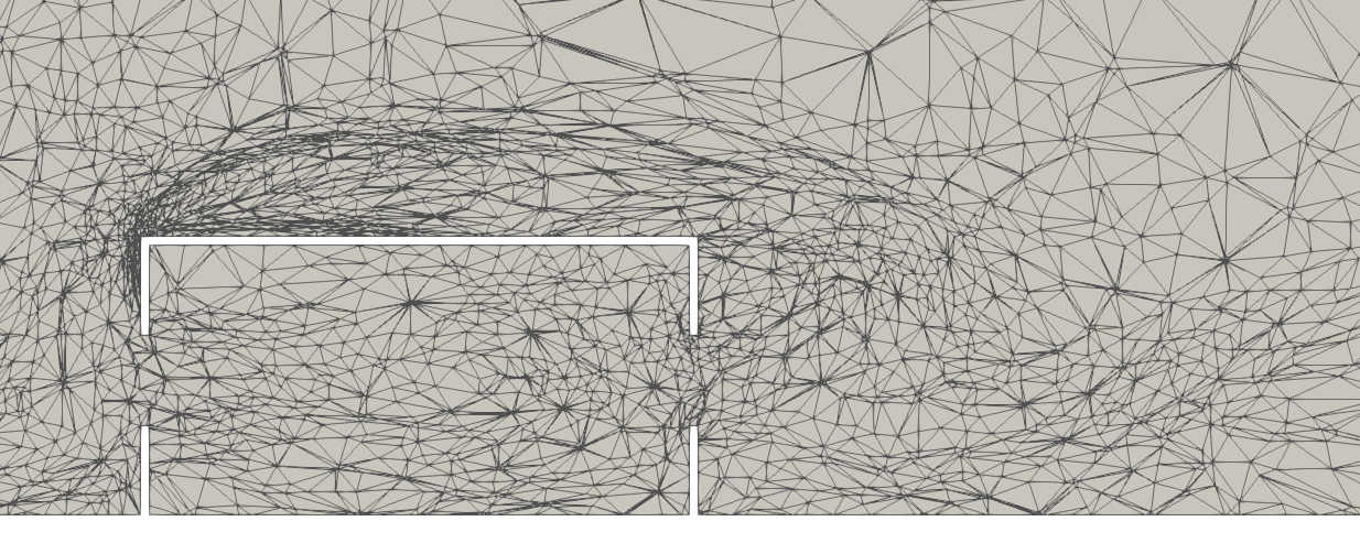
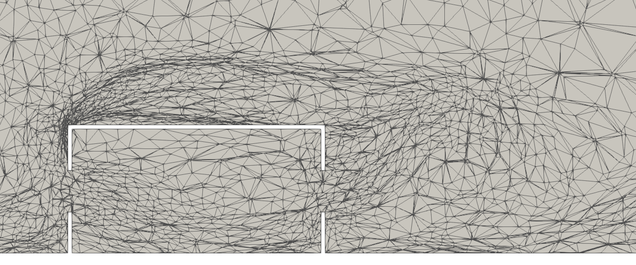
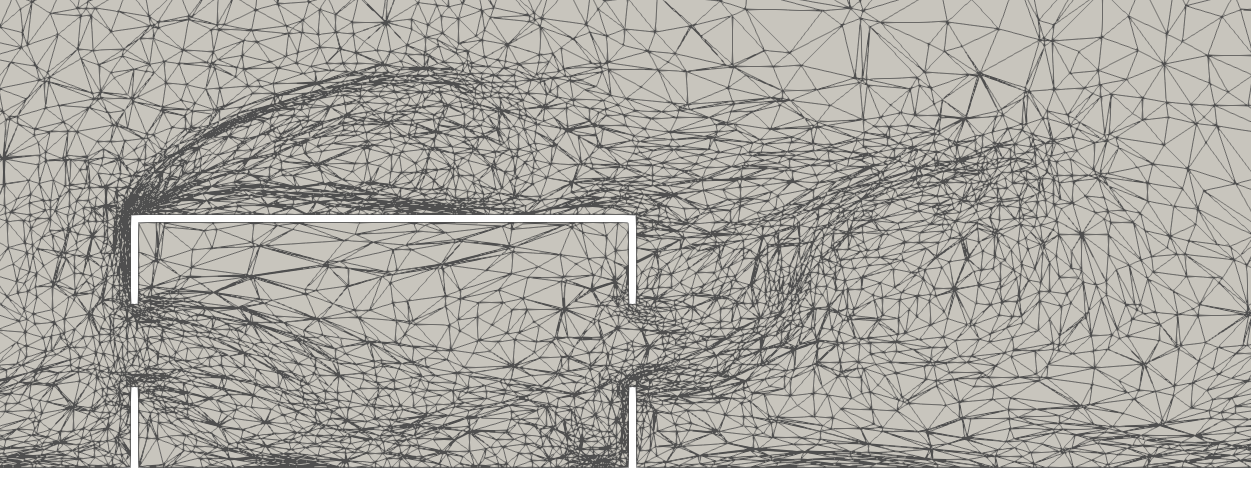
Snapshots of the meshes are shown in Figure 5.27. Snapshots of the temperature field are shown in Figure 5.28. Snapshots of the velocity field are shown in Figure 5.29. Go to Chapter 10 to learn how to visualise the results using ParaView.
As shown in Figure 5.27 the mesh is well-adapted based on the velocity field, i.e. at the openings and around the exterior surfaces of the box and based on the temperature field, i.e. within the box. In other words, the mesh is not only adapted in the interior or the exterior of the box but in both regions, thus capturing the full dynamics of the velocity field and the temperature field.

5.3.5 Computation time
The computation time for all the simulations is reported in Table 5.2, highlighting that refining the mesh, i.e. decreasing the error_bound_interpolation, drastically increases the computational time. Therefore, a trade-off has to be made between the accuracy desired and an acceptable computational time.
|
Case
Nbr |
Simulation
time: 2 s |
Simulation
time: 6 s |
Simulation
time: 9 s |
Simulation
time: 40 s |
|---|---|---|---|---|
| 6a | 00H 01min 05s | 00H 01min 33s | 00H 01min 53s | 00H 02min 08s |
| 6b | 00H 01min 35s | 00H 02min 59s | 00H 04min 27s | 00H 32min 29s |
| 6c | 00H 25min 12s | 01H 24min 33s | 02H 11min 44s | 16H 51min 14s |
| 6d | 03H 43min 19s | 10H 28min 17s | 19H 19min 28s | Too long… |
| 7a | 00H 02min 39s | 00H 03min 38s | 00H 04min 12s | 00H 09min 56s |
| 7b | 00H 07min 37s | 00H 11min 42s | 00H 16min 45s | 01H 21min 22s |
| 7c | 00H 25min 37s | 00H 58min 26s | 01H 34min 29s | 08H 25min 53s |
| 7d | 01H 04min 17s | 02H 35min 45s | 03H 56min 29s | 31H 04min 48s |
| 8 | 00H 32min 27s | 01H 10min 05s | 01H 50min 02s | 11H 08min 00s |
5.4 Ensuring enough resolution in specific region
5.4.1 Python script to refine zone
Boundary conditions
For the cases 3dBox_Case9a.flml and 3dBox_Case9b.flml, the initial and the ambient temperatures are set to 293 K and is set to m/s. The heat flux applied at the source is equal to 1000 W/m2, hence , set up in Diamond, is equal to 0.8163 according to equation 4.1. The surface of the heat source is m2: the flux applied at the source is then equal to 40 W. This example is similar to 3dBox_Case2b.flml which is set up without mesh adaptivity, i.e on a fixed mesh.
CFL number
To avoid any crash of the simulations, the time step is now also adaptive using a CFL condition as described in Section 3.2.2, with the CFL number taken as 2 in the following example. This value can be increased later on to speed up the simulations. However, it is recommended to do a sensibility analysis of the results as a function of the CFL number to ensure that no important information is missed. Moreover, a maximum time step is prescribed equal to 1 s: at the beginning of the simulation, the velocity within the domain is almost equal to 0 m/s. As a consequence, based on the CFL number, the computed time step will be unreasonably very large (see equation 3.11) causing the simulation to crash.
General mesh adaptivity options
In the following sections, mesh adaptivity will be performed based on the temperature and the velocity fields. The maximum number of nodes is set to and the mesh is adapted every 10 time steps.
Based on the results of 3dBox_Case2b.flml, the velocity is estimated to be approximately between 0 m/s and 0.45 m/s. The velocity error_bound_interpolation is taken to be equal to 10% of the velocity range, i.e equal to 0.045. Based on the results of 3dBox_Case2b.flml, the temperature is estimated to be approximately between 293 K and 333 K. However, the highest temperatures are located near the source only: the rest of the inner box is much cooler, i.e. between 293 K and approximately 300 K. The choice is then made not to take into account the entire temperature range, but only the one of interest, i.e. between 293 K and 300 K. The temperature error_bound_interpolation is taken to be equal to 10% of the interesting temperature range, i.e of 7 K. Therefore, the error_bound_interpolation is set to 0.7.
Minimum and maximum edge lengths
The characteristic length of the domain is taken to be the windows opening, i.e. : the minimum edge length is set up to , i.e. 0.01 m. The height of the domain is 21 m: the maximum edge length is set up to , i.e 2.1 m.
As shown in Figure 5.30, these error_bound_interpolation values gives acceptable results as a first run. However, zooming on the source, Figure 5.31 shows that the region near the source is not well resolved. It is commonly assumed that at least 10-20 elements should define a source, which is clearly not the case in 3dBox_Case9a.flml.


Reducing the error_bound_interpolation value for the temperature will have a tendency to overly increase the resolution near the source at the expense of the rest of the plume. One shortcut, to ensure a well resolved source, is to use a python script to vary the specified minimum and the maximum edge lengths over the domain, constraining finer resolutions over areas of interest, in this case the source. It is worth noting that this technique can also be used to ensure refinement near openings for example. In example 3dBox_Case9b.flml, the python scripts in Code 1 and Code 2 are used to set up the minimum and the maximum edge lengths. The refined region of the mesh near the source is twice as large as the source itself and at least 20 elements are forced in that region. The mesh obtained near the source is shown in Figure 5.31(d).
These two python scripts can be used for a square/cubic source. For a circular/spherical/ellipsoidal source, a python script similar to the one in Code 3 can be used.
These examples can be run using the commands:
Go to Chapter 10 to learn how to visualise the results using ParaView.
5.4.2 Locking nodes
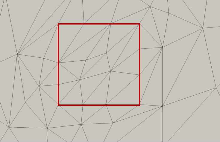
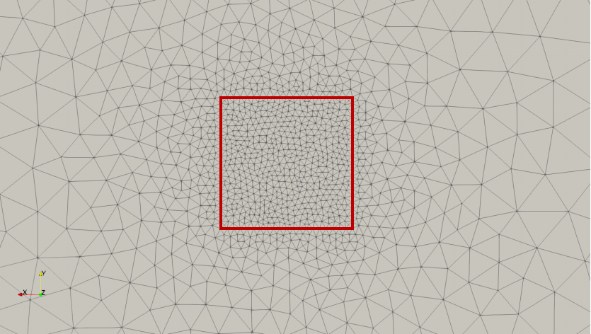
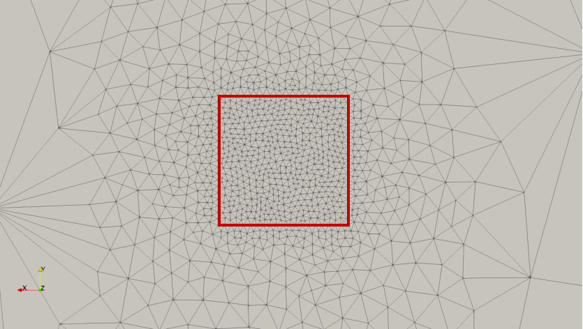
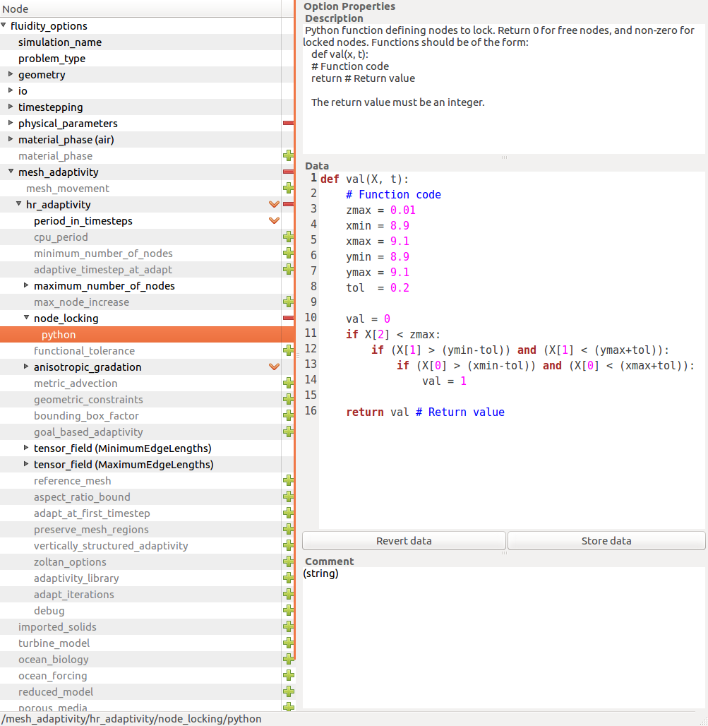
Set-up of example 3dBox_Case9c.flml is the same than example 3dBox_Case9a.flml. In example 3dBox_Case9c.flml, the Box.geo and by consequence Box.msh files were modified to initially assign an higher resolution near the source as shown in Figure 5.32(a). In the mesh adaptivity option, the option node_locking (Figure 5.33) is turned on to specify that nodes around the source are locked using Code 4. This option prevent the mesh to be adapted where specified and thus allow to ensure that the desire resolution in specific regions are kept. Once the simulation is running, it can be observed that the mesh is preserved at the source location after the adaptation process (Figure 5.32(b)). However, this option can sometimes lead to weird meshes.
This example can be run using the command:
Go to Chapter 10 to learn how to visualise the results using ParaView.
5.5 Advection of the mesh
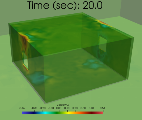
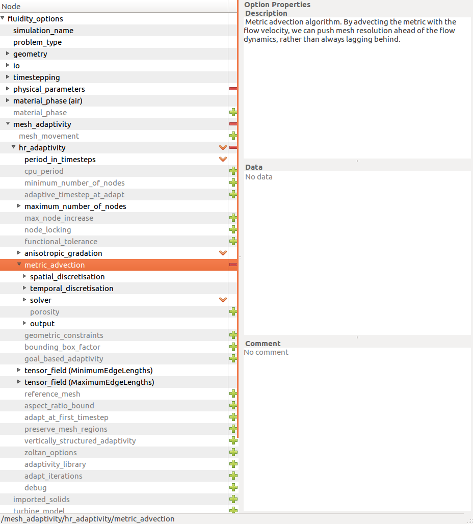
Metric advection is a technique that uses the current flow velocity to advect the metric forward in time over the period until the next mesh adapt. With metric advection, mesh resolution is pushed ahead of the flow such that, between mesh adapts, the dynamics of interest are less likely to propagate out of the region of higher resolution. This leads to a larger area that requires refinement and, therefore, an increase in the number of nodes. However, metric advection can allow the frequency of adapt to be reduced whilst maintaining a good representation of the dynamics.
The options for metric advection can be found under the mesh_adaptivity options as shown in Figure 5.34. The advection equation is discretised with a control volume method. For spatial discretisation, a first order upwind scheme and non-conservative (conservative_advection=0) form are generally recommended. For temporal discretisation a semi-implicit discretisation in time is recommended, i.e theta=0.5. The time step is controlled by the choice of CFL number under the option temporal_ discretisation/maximum_courant_number_per_subcycle and the value set should be the same as the one specified under the option timestepping /adaptive_timestep/ requested_cfl.
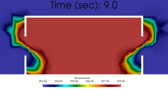
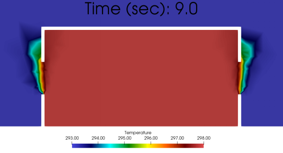
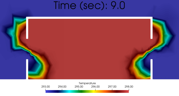
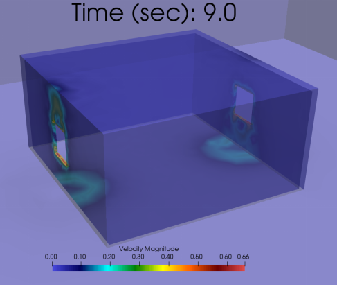
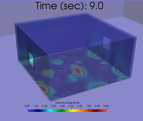
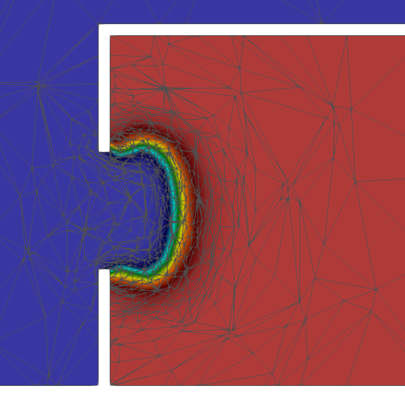
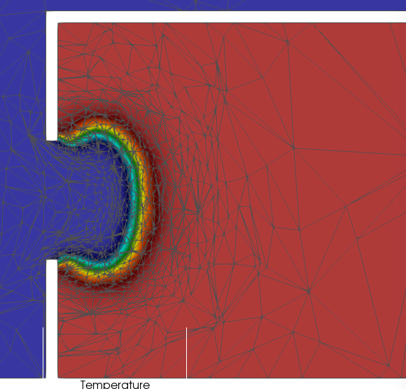
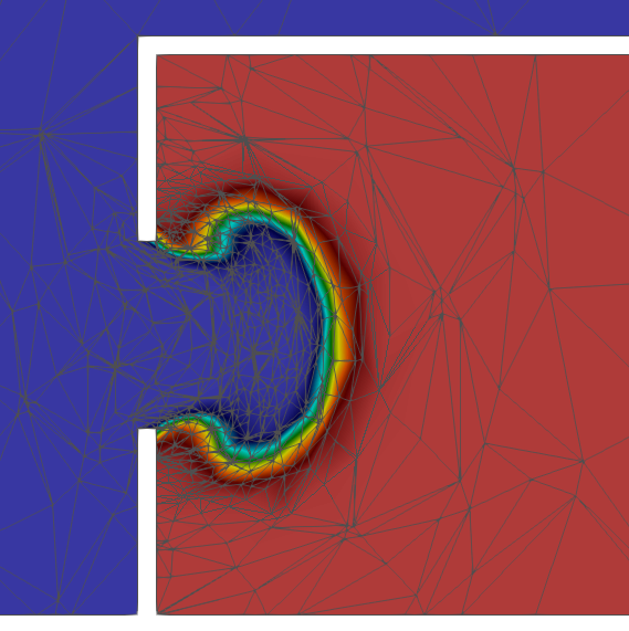
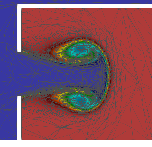
The case 3dBox_Case10.flml is similar to the case 3dBox_Case6c.flml with the mesh advection turned on. Difference between the meshes generated at different times for both cases is shown in Figure 5.35 and Figure 5.36. Figure 5.35 shows the meshes and the temperature field just after the second adaptation and just before the third adaptation. The region where the mesh is refined in Figure 5.35(a) is clearly much smaller than in Figure 5.35(b). Therefore, just before the next adaptation, the temperature starts to propagate out of the region with higher resolution when mesh advection is not used, as shown in Figure 5.35(c). However, the temperature is maintained in the finer region when using the mesh advection option as shown in Figure 5.35(d).
Figure 5.36 shows the temperature field at 1 s. As the advection of the mesh allows the field of interest to remain in the fine region, there should be less artificial diffusion due to the presence of coarse mesh elements as shown in Figure 5.36.


5.6 Common errors
All errors are listed in the fluidity-err.0 file, including those linked to mesh adaptivity. Some might only be warnings and if the simulation is still running they can be safely ignored. However, if something went wrong during the adaptation process, the simulation will automatically crash. This is primarily caused by the user pushing the adaptation parameters too far… Finally, the user should be reminded that it is not recommended to adapt the pressure field.
Chapter 6 Other fields
6.1 Case set-up
Example 3dBox_Case11.flml is based on example 3dBox_Case8.flml, apart from the following properties that were changed to speed-up the simulation:
-
•
CFL number is now equal to 5.
-
•
Mesh adaptivity options:
-
–
Temperature: error_bound_interpolation=0.2
-
–
Velocity: error_bound_interpolation=0.17
-
–
The mesh is advected.
-
–
The mesh is also refined at the openings of the box, using a python script in the maximum edge length field under the adaptivity option, to be sure that the flow is well-captured (Figure 6.1(c)).
A number of other fields can be added in Diamond and some are described below. Example 3dBox_Case11.flml contains all the interesting fields discussed in this chapter and that the user might want to use. The fields in 3dBox_Case11.flml are the following:
-
•
Prognostic fields:
-
–
Pressure
-
–
Velocity
-
–
Temperature
-
–
Tracer
-
–
-
•
Diagnostic fields:
-
–
Density
-
–
VelocityAverage: time-average of the velocity
-
–
u: , fluctuation term of the -component of the velocity
-
–
v: , fluctuation term of the -component of the velocity
-
–
w: , fluctuation term of the -component of the velocity
-
–
uu: , squared fluctuation term of the -component of the velocity
-
–
vv: , squared fluctuation term of the -component of the velocity
-
–
ww: , squared fluctuation term of the -component of the velocity
-
–
uuAverage: , -component of the Reynolds stresses (time-average)
-
–
vvAverage: , -component of the Reynolds stresses (time-average)
-
–
wwAverage: , -component of the Reynolds stresses (time-average)
-
–
PressureAverage: time-average of the pressure
-
–
TemperatureAverage: time-average of the temperature
-
–
TracerAverage: time-average of the passive tracer
-
–
CFLNumber: CLF number in the mesh
-
–
EdgeLength: edge length in the domain
-
–
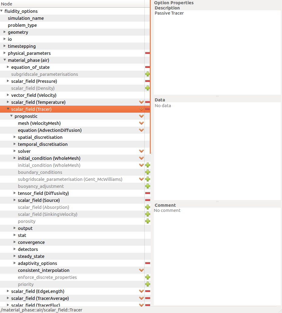
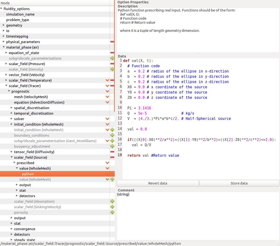
6.2 Passive tracer
A passive tracer field can notably be added as shown in Figure 6.1. In example 3dBox_Case11.flml, the passive tracer has a source located in the middle of the box. Let’s assume that the passive tracer is , the diffusion coefficient of in air is equal to m2/s. A source, located in the middle of the box, is assumed to release with a mass flow rate equal to kg/s. The volume of the source is assumed to be half a sphere with a radius of m. Therefore, based on equation 3.6 and equation 3.8, the python script in Code 1 is assigned to the source scalar field in the Tracer field. Moreover, the mesh in the vicinity of the source is forced to be refined using python scripts, as previously described.

6.3 Diagnostic fields in Diamond
Some interesting diagnostic fields can also be added in Diamond. Diagnostic fields are calculated from other fields without solving a partial differential equation. Note that scalar, vector and tensor diagnostic field can be added, but only the interesting scalar and vector ones are discussed here.
6.3.1 Density field
The density field is automatically available in Diamond like the Pressure and the Velocity ones, except it is turned off by default. The user can turn on this field if wanted.
6.3.2 Diagnostic fields
See Chapter 9 of Fluidity manual [1] for more details.
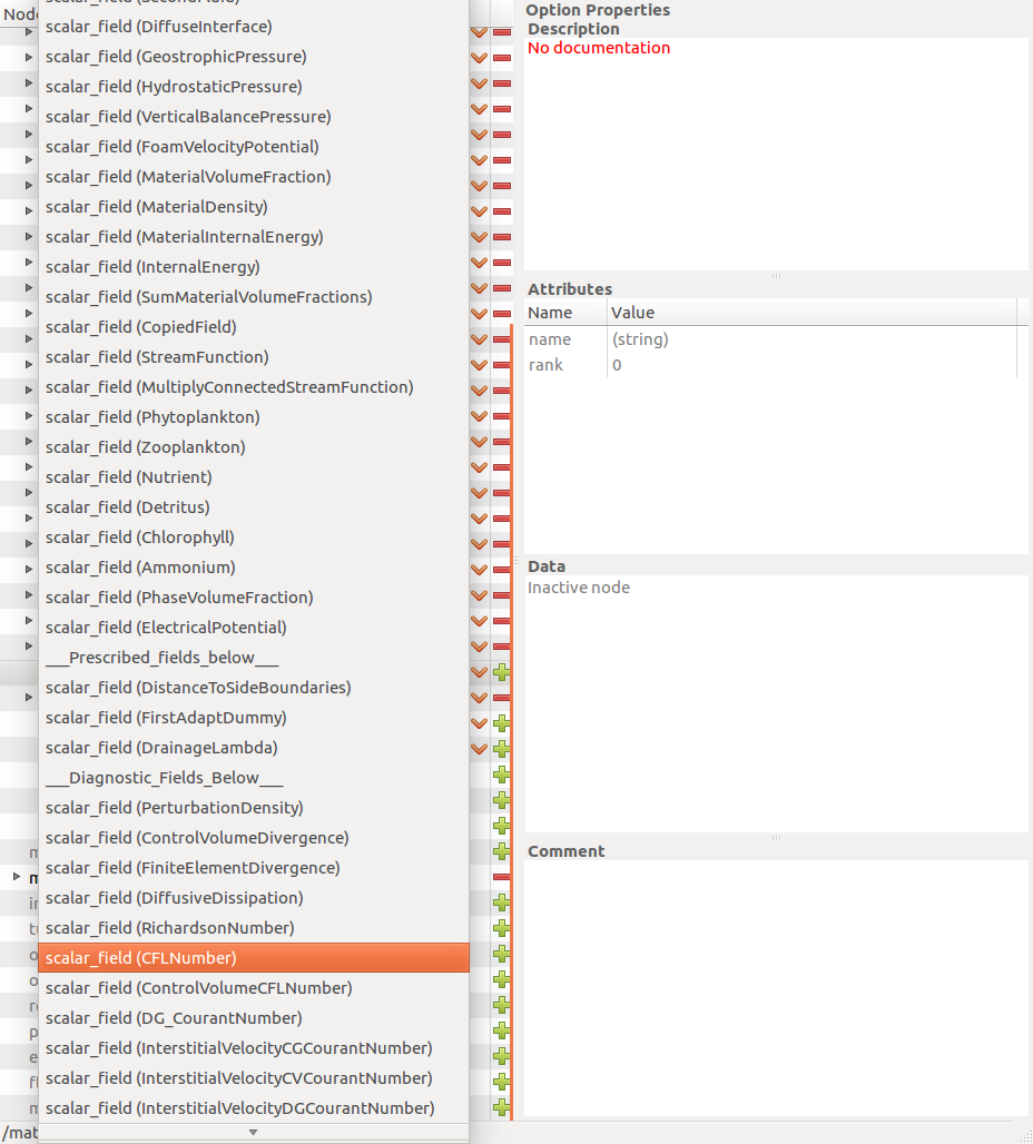
As shown in Figure 6.2, already implemented diagnostic fields can be found in several locations in Diamond:
- •
-
•
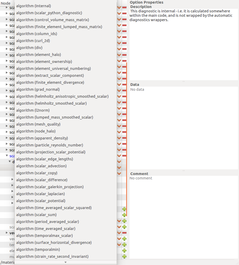
Diagnostic algorithms: Add a new scalar or vector field, then open the option tree and choose diagnostic instead of prognostic. Under the diagnostic option, the user will see the algorithm, set by default to internal. Here, the algorithm can be changed into another using the drop down list as shown in Figure 6.2(c) and Figure 6.2(d).
Internal diagnostic fields
The scalar field to output the CFL number is for example already implemented as a scalar field as shown in 6.2(a). In the same list, the user can notice that it is also possible to output the grid Reynolds number and the grid Peclet number.
Diagnostic algorithms
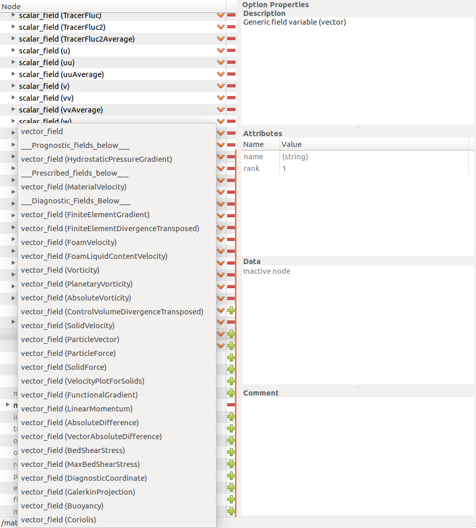
Once a new scalar or vector filed is added and diagnostic is chosen, the user can notice other interesting diagnostic fields (Figure 6.2(c) and Figure 6.2(d)) such as:
-
•
time_averaged_scalar: calculates the time-average of a scalar field over the duration of a simulation. A spin-up time can be added: the average will start after the set-up value (value in second).
-
•
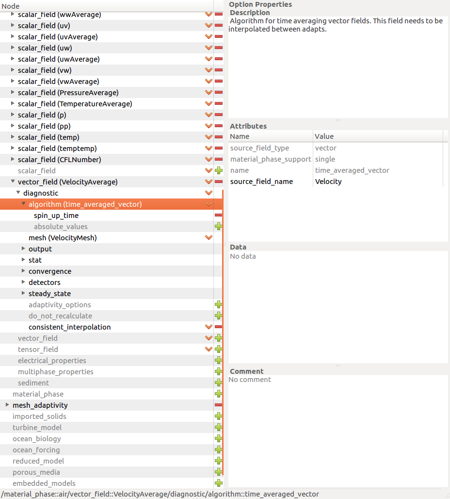
time_averaged_vector: calculates the time-average of a vector field over the duration of a simulation. A spin-up time can be added: the average will start after the set-up value (value in second).
-
•
scalar_edge_lengths: outputs the edge lengths of the mesh.
-
•
scalar_python_diagnostic: allows direct access to the internal Fluidity data structures in the computation of a scalar diagnostic field.
-
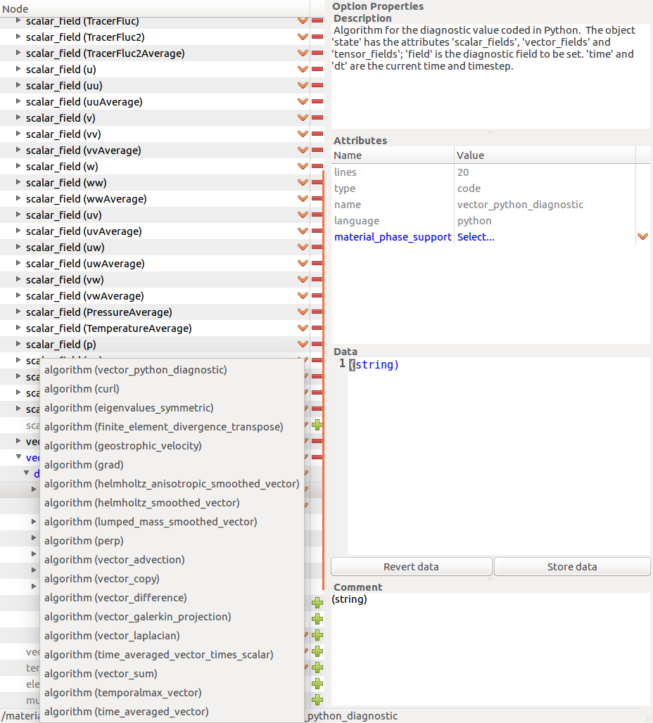
•
vector_python_diagnostic: allows direct access to the internal Fluidity data structures in the computation of a vector diagnostic field.
Some diagnostic algorithms need a source field attribute defining the field used to compute the diagnostic (for example the field used to compute the time-average). The name of the field as to be set appropriately, see Figure 6.3(a) for example.
By selecting the scalar_python_diagnostics or vector_python_diagnostic options, a python script can be used to calculate a new field from existing fields. Under the option depends, the user can specify dependencies manually. Any field specified here will be calculated before the python diagnostic field. An example is shown in Figure 6.3(b) where the instantaneous component is calculated directly from the velocity field and its time-average. The python code to compute the instantaneous value is shown in Code 2. Then, applying the time_averaged_scalar to this field will give the -component of the Reynolds stresses.

6.3.3 Note about the time-averaged field
Note that there is currently a bug in Fluidity concerning the time-averaged field: when a simulation is run from a checkpoint the value of the previous time-average is not properly read from the checkpointed files implying that the average is not correct. This will later be fixed but for now it is recommended to the user to specify a spin-up time higher than the checkpoint time to start a new time-average. See Section 8.7 for more details about checkpointing.
For the time averaged fields, when using adaptivity, it is also recommended to use the galerkin_projection option instead of the consistent_interpolation one, more details are given in Section 8.5.
Chapter 7 Details of options
A number of options for the simulation are available to be set up in Diamond. Some are detailed here and most are described in the manual too [1]. For simplicity a screen shot of the drop down menu found in Diamond is shown in Figure 7.1. The name of the simulation is inputted in simulation_name and the problem type is defined as fluids for the cases considered here.
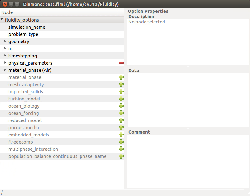
7.1 Geometry
The first part of the options defines the geometry used for the simulations as shown in Figure 7.2. The file used for the mesh needs to be inputted in mesh (CoordinateMesh) /from_file.
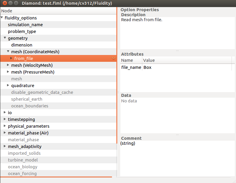
7.2 Input-Output
The options for the inputs and outputs are defined in the io menu shown in Figure 7.3.
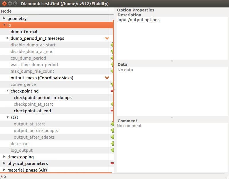
In these options, dump_period_in_timesteps defines how often ParaView files (*.vtu) should be outputted. This can be defined as a function of time (in second) or time steps.
The checkpointing options are also defined in this section. They will determine how often checkpoints are made. Checkpoints will become useful if a simulation needs to be restarted from a particular point in time. See Section 8.7 for more details.
7.3 Time stepping
The options for time stepping are then defined in the timestepping menu shown in Figure 7.4. They comprise the initial, current and final time of the simulation as well as the time step requested, and are all defined in seconds. In the case of an adaptive time step, this is the initial time step. The adaptive time step can be turned on by selecting the option and choosing a CFL number under requested CFL. The non-linear iteration parameter has to be set equal to 2.
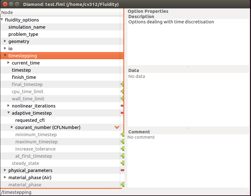
7.4 Physical parameters
The magnitude and direction of gravity is defined in the drop down menu of the physical parameters shown in Figure 7.5. It is valuable to check whether the value of gravity corresponds to the coordinate system used. For example, the magnitude is usually set to 9.81 (if you are not on Mars) and the GravityDirection to if the -axis corresponds to the height pointing upwards.
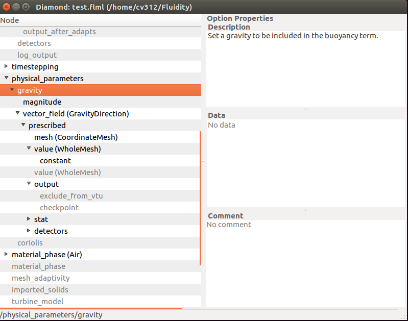
7.5 Material phase
All the fields used for a given fluid are defined in material_phase/, this include their initial and boundary conditions. In a case where different materials are used multiple material_phase/ sections will have to be added. In the cases presented here however, only air is present.
7.5.1 Equation of state
The equation of state options, shown in Figure 7.6, define the dependency between temperature and density. This is also where the reference values for temperature and density are defined. The option subtract_out_hydrostatic_level has to be turned on if the Boussinesq approximation is used, which is the case in all the examples presented in this manual.
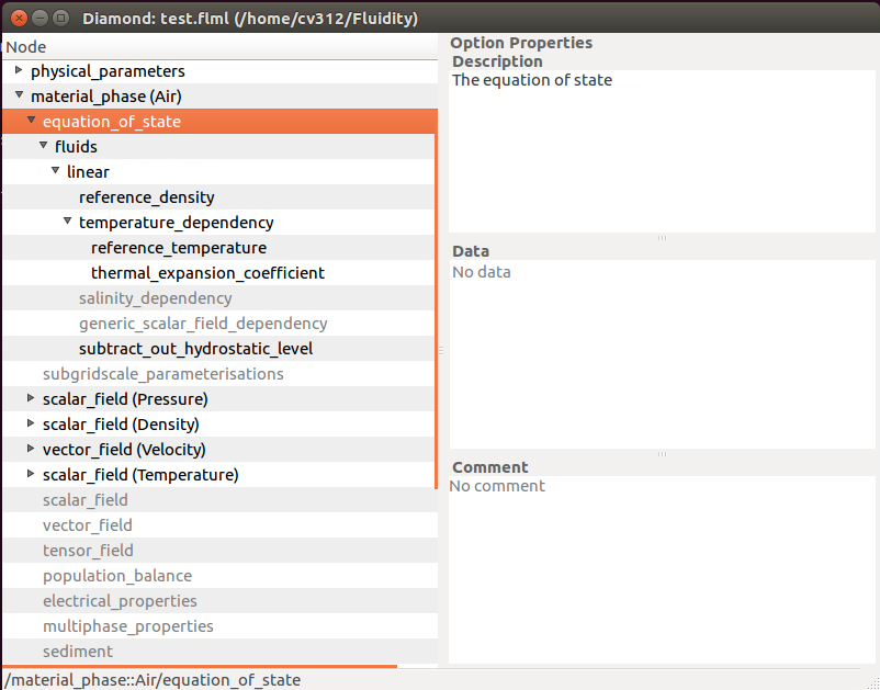
7.5.2 Prognostic fields
The prognostic scalar_field and vector_field are used to define certain fields such as pressure and velocity as shown in Figure 7.7.
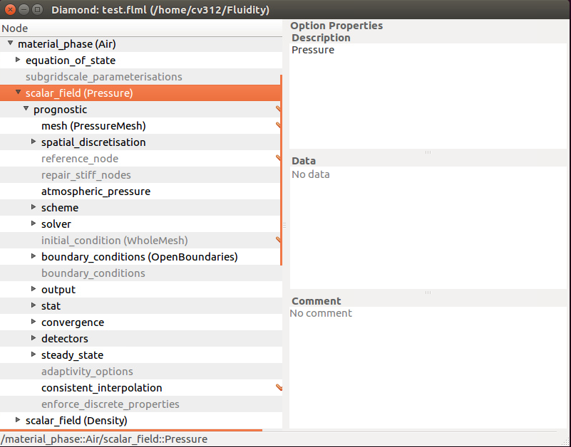
This is where boundary and initial conditions are defined as well as how each field is discretised and solved. Output options are also available. Finally adaptivity_options will allow to define the interpolation error bound used as a weight during the adaptivity process. The following options are chosen for the main prognostic fields.
For the pressure field:
-
•
Spatial discretisation: continuous_galerkin.
-
•
Scheme: poisson_pressure_solution with a use_projection_method.
-
•
Solver: iterative_method (cg) with a preconditioner (hypre) and hypre_ type (boomeramg). Other options are relative_error and max_iterations with the suggested values as well as adding the never_ignore_solver_failures.
For the velocity field:
-
•
Spatial discretisation: continuous_galerkin, including the options
-
–
stabilisation/no_stabilisation
-
–
mass_terms/lump_mass_matrix
-
–
stress_terms/tensor_form
-
–
les_model/second_order (with a Smagorinsky coefficient of 0.1 and a tensor length_scale_type)
-
–
-
•
Temporal discretisation: with a theta of 0.5 and relaxation of 0.5.
-
•
Solver: iterative_method(gmres) and preconditioner (sor). Other options are relative_error and max_iterations with the suggested values as well as adding the never_ignore_solver_failures.
For the temperature field:
-
•
Spatial discretisation: control_volumes with a face_value(FiniteElement) of limit_face_value specified by a limiter(Sweby). The diffusion_scheme is ElementGradient and the conservative_advection is set to 0.
-
•
Temporal discretisation: theta is 0.5. The control_volumes option is selected with a number_advection_iterations set to 2.
-
•
Solver: iterative_method(gmres) and preconditioner (sor). Other options are relative_error and max_iterations with the suggested values as well as adding the never_ignore_solver_failures.
7.5.3 Diagnostic fields
The material_phase section also includes the calculated diagnostic fields as shown in Figure 7.8. See Section 6.3 for more details.
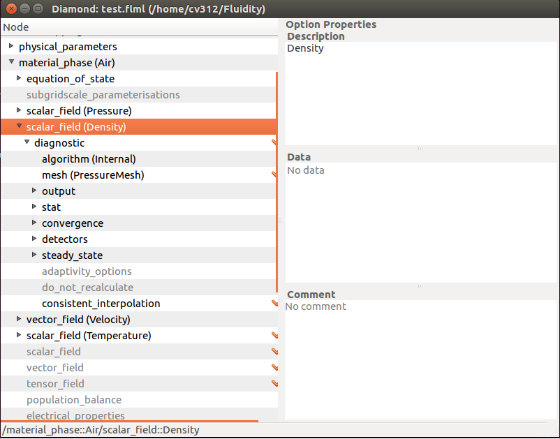
7.6 Mesh adaptivity
This section defines the adaptivity process and how it will be conducted. The available options are shown in Figure 7.9 for the chosen hr_adaptivity algorithm.
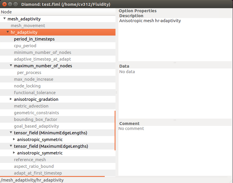
In particular, period_in_timesteps allows to define how often adaptivity is to happen, anistropic_gradation how the mesh should be smoothed out, while maximum_number_ of_nodes sets an upper bound on the number of nodes the mesh can be decomposed into. As a rule of thumb it is recommended to use at least 50,000 nodes per processor.
Finally, the minimum and maximum edge lengths can also be defined in this section. In combination with the interpolation error bound they will define how the resolution of the mesh will vary with adaptation. Python scripts can be used to vary the specified lengths over the domain, allowing finer resolutions over areas of interest for instance. More details on the adaptivity process can be found in Chapter 5.
Chapter 8 Tricks
8.1 Size of the domain
8.1.1 Blockage ratio
The size of the computational domain has to be properly chosen and it is recommended for the user to read carefully [7] for a detailed method. The following summarises the principal rule of thumb and basically paraphrases [7]. First, let’s define the blockage ratio as expressed by equation 8.1:
| (8.1) |
where is the projected area of the building in flow direction and is the inlet area.
In the case of a single building: , where is the width of the building and its height. In the case of multiple buildings: , where is the average diameter of the domain of interest and is the height of the tallest building.
8.1.2 Height of the domain
To prevent artificial acceleration of the flow over the building, the height of the domain has to be chosen as follows.
-
•
For a single building: the top of the computational domain should be at least above the roof of the building. To eliminate errors due to the size of the computational domain, the blockage ratio is recommended to be lower than 3% in CFD simulations.
-
•
For urban environment with more than one building: the top of the computational domain should be at least above the tallest building.
Based on the blockage ratio, smaller and larger values can be used: is sufficient for a small blockage, while is recommended for a large blockage.
If the simulations are to be compared with wind tunnel experiments, it is recommended to use the wind tunnel’s test section geometry for the computational domain. However, if the height of the wind tunnel is much larger than , then a lower height of the computational domain can be tested.
8.1.3 Width of the domain
Once the height of the domain is defined, the width of the domain can be determined using the blockage ratio formula.
-
•
For a single building: assuming a domain height of the requirement of 3% blockage leads to a distance of between the building’s side and the lateral boundaries of the computational domain. The published recommendations for this distance are however much larger and using , leading to a blockage of only 1.5%, is recommended.
-
•
For urban environment with more than one building: the lateral boundaries of the computational domain can be placed closer than from the built area.
If the simulations are to be compared with wind tunnel experiments, it is recommended to use the wind tunnel’s test section geometry for the computational domain. However, if the lateral walls of the wind tunnel from the built area is much larger than , then a smaller width of the computational domain can be tested.
8.1.4 Length of the domain
The length of the domain has to be divided into two regions:
-
•
The upstream region:
-
–
For a single building: a distance of between the inflow boundary and the building is recommended.
-
–
For urban areas: a distance of between the inflow boundary and the building is recommended.
-
–
-
•
The downstream region:
-
–
For a single building: a distance of again behind the building is recommended.
-
–
For urban areas: a smaller distance between the outflow boundary and the built area can be used.
-
–
Large values are recommended for the downstream region to avoid flow entering the domain through the outflow boundary. Indeed, this situation should be avoided as it can lead to the divergence of the solver and the crash of the simulation. However the recommended value of can lead to too big domain that will increase considerably your computational time. Solutions to tackle this issue are discussed in the next Section 8.2.
8.2 Instabilities at the edges of the domain
Running example 3dBox_Case12a.flml long enough, the user can observe that the simulation starts to behave weirdly around 74 seconds and finally crashes at 87 seconds. The user can test this example easily, it takes only 8 minutes to run until crashing. As shown in Figure 8.1, very high and unrealistic velocity magnitudes appear at the outlet of the domain: this is due to turbulent recirculation at the outlet which causes numerical instabilities until the divergence of the solver. This is a well-known numerical issue which unfortunately occurs often. There are two ways to avoid this issue:
-
•
Extend the length of the domain as far as needed. This should be the first option to consider.
-
•
Add a ‘sponge’ layer at the end of the domain to artificially dissipate the eddies.
To avoid any unwanted recirculation and/or instabilities occurring at the domain edges, the user can add a so-called ‘sponge’ layer which will stabilise the turbulent flow and suppress the eddies. When using this solution, it is recommended to the user to be sure that the results in the domain of interest are not affected by the ‘sponge’ layer, i.e to be sure that the killed turbulence does not have a direct impact and repercussion on the results. The ‘sponge’ layer is prescribed through a python script and there are two ways to define it:
-
•
Viscosity layer: the value of the viscosity is linearly increased at the end of the domain as shown in Figure 8.2(a). In the velocity field, the python script in Code 1 is used to prescribe the viscosity: the viscosity increases linearly from the typical value for air of m2/s to several orders of magnitude higher. The user can refer to example 3dBox_Case12b.flml. This example runs properly and no instabilities occur anymore at the outlet as shown in Figure 8.2.
1def val(X, t):2 # Function code3 # Viscosity values4 nu = 1.5e-5 # Value of viscosity in the domain5 nuMax = 0.15 # Maximum value of the viscosity67 # Geometry variables8 xMax = 21.0 # Length of the domain9 Llayer = 2.0 # Length of the layer - in meter10 xStart = xMax - Llayer # Where to start the sponge layer1112 # Viscosity Ramp x-Direction ------ viscosity = a*x+b13 a = (nuMax - nu)/(xMax - xStart) # Slope14 b = nu - a * xStart1516 val = nu17 # Assigning an increased value of viscosity near the outlet18 if (X[0] >= xStart):19 val = a * X[0] + b2021 return val #Return valueCode 1: Python script to define an increasing viscosity at the outlet of the domain. -
•
Absorption layer: an absorption term is prescribe at the end of the domain as shown in Figure 8.3(a). In the velocity field, the python script in Code 2 is used to prescribe an absorption term: the absorption is equal to zero in the domain and increases linearly to . The latest value will have to be adjusted by the user depending of the case used. The user can refer to example 3dBox_Case12c.flml. This example runs properly and no instabilities occur anymore at the outlet as shown in Figure 8.3.
1def val(X, t):2 # Function code3 # Absorption values4 AMin = 0.0 # Value of the absorption in the domain equal to zero.5 AMax = 0.25 # Maximum value of absorption67 # Geometry variables8 xMax = 21.0 # Length of the domain9 Llayer = 2.0 # Length of the layer - in meter10 xStart = xMax - Llayer # Where to start the sponge layer1112 # Absorption Ramp x-Direction ------ absorption = a*x+b13 a = (AMax - AMin)/(xMax - xStart) # Slope14 b = AMin - a * xStart1516 val = [AMin, 0, 0]17 # Assigning an absorption term near the outlet18 if (X[0] >= xStart):19 val = [a * X[0] + b, 0, 0]2021 return val #Return valueCode 2: Python script to define an absorption term at the outlet of the domain.
The difference of what is happening at the outlet of the domain when using a viscosity or an absorption layer can be seen in Figure 8.2 and Figure 8.3, and the authors leave the users to appreciate which one in the more suitable for their application.
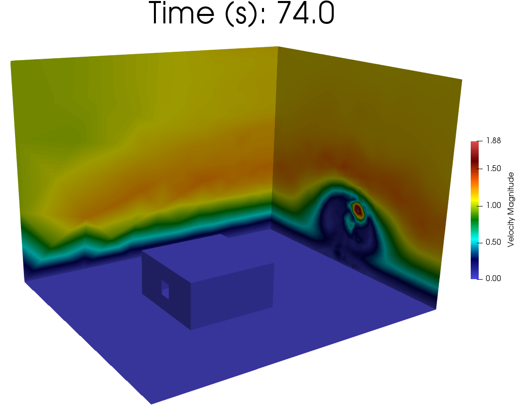
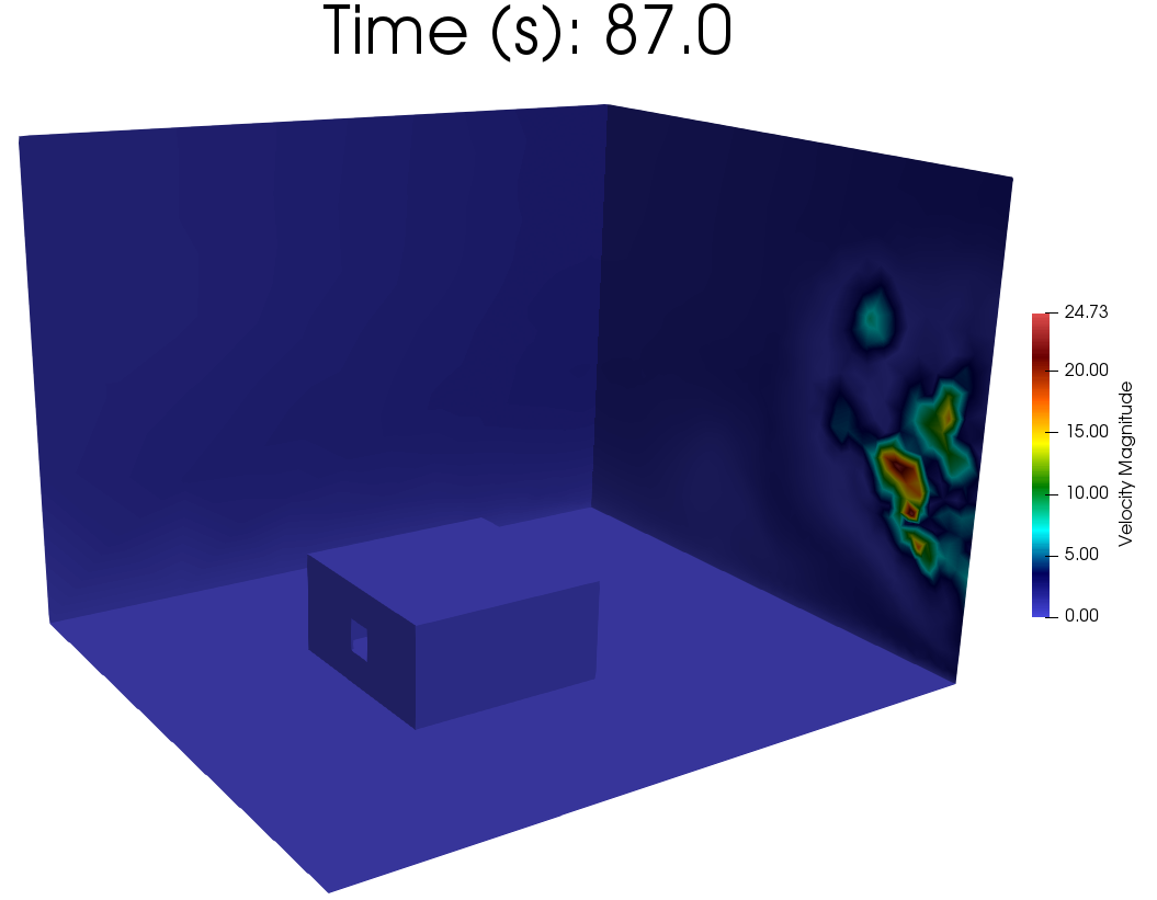
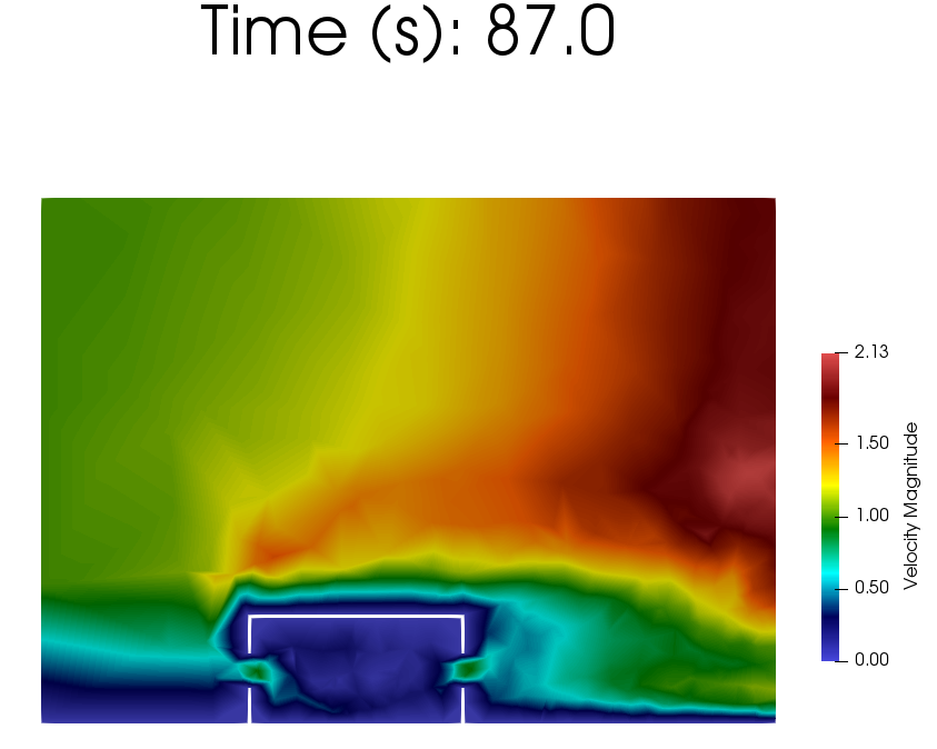
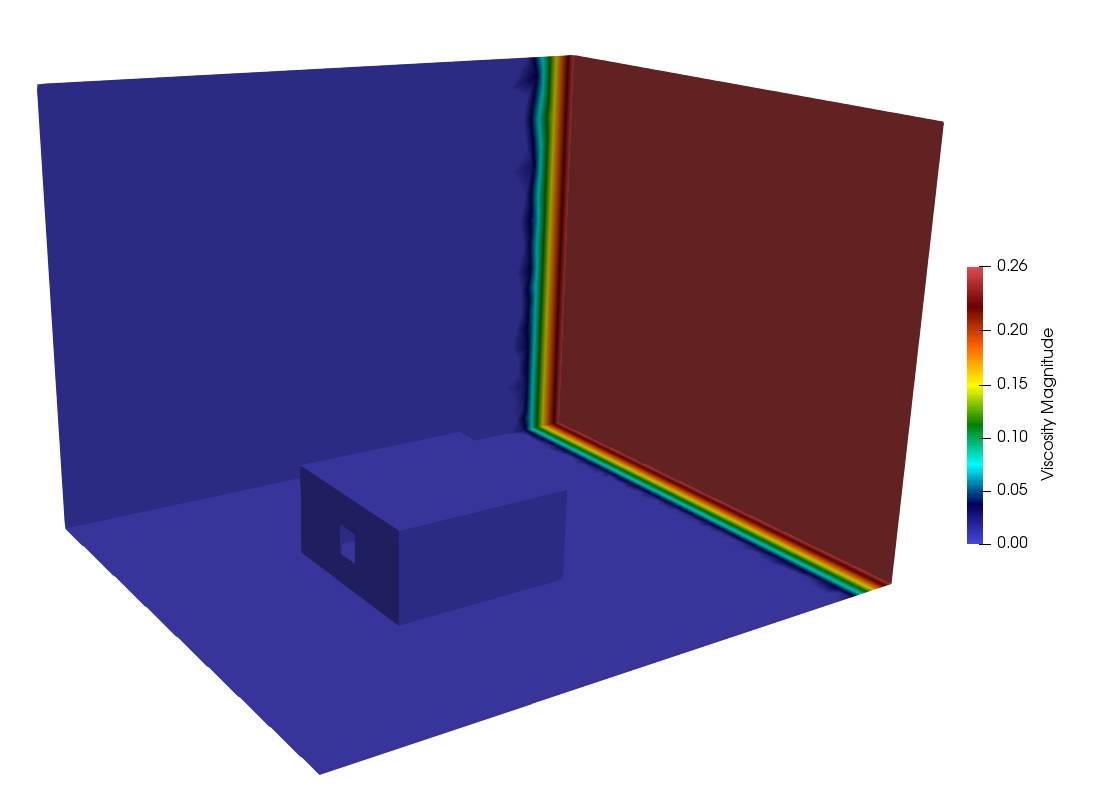
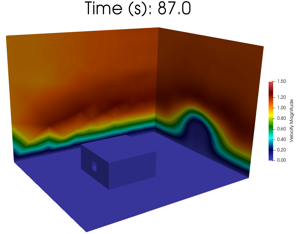
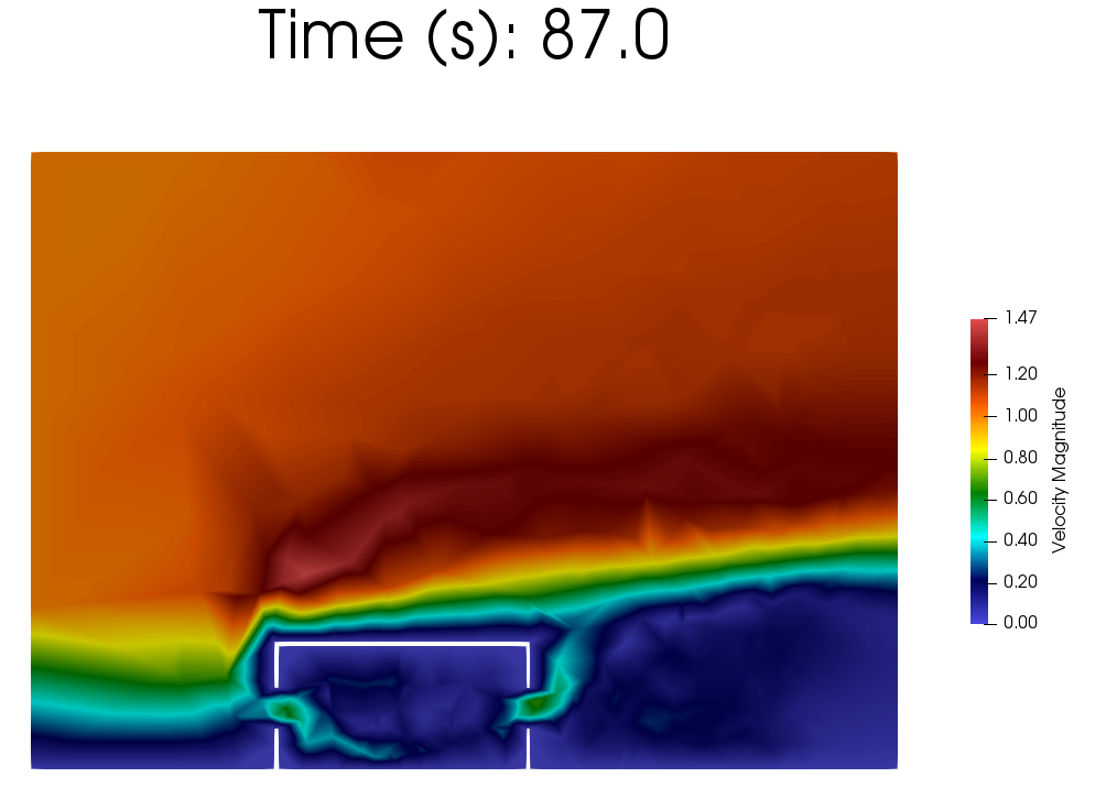
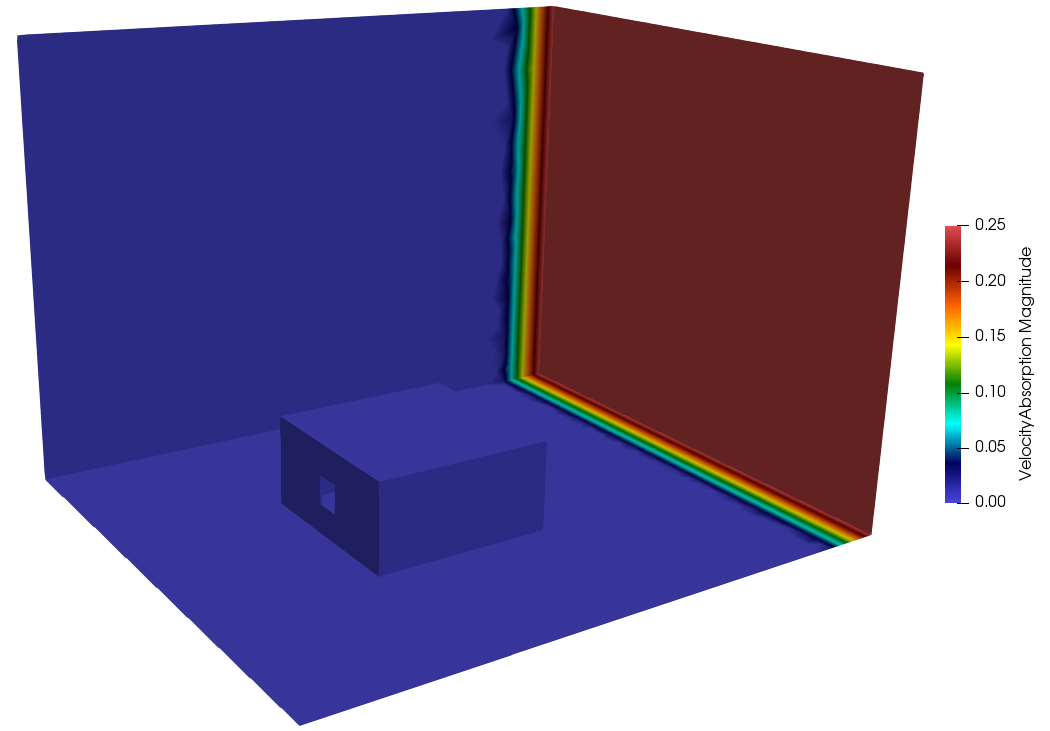
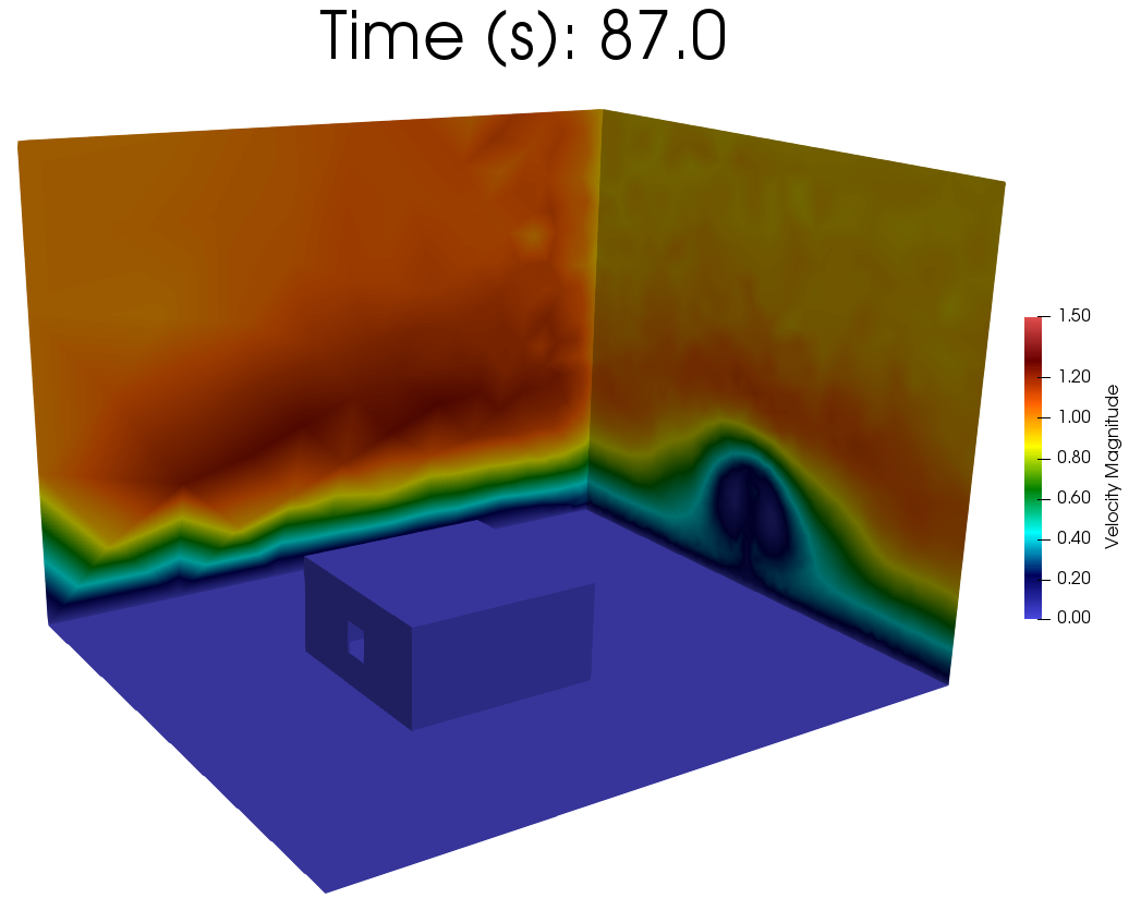
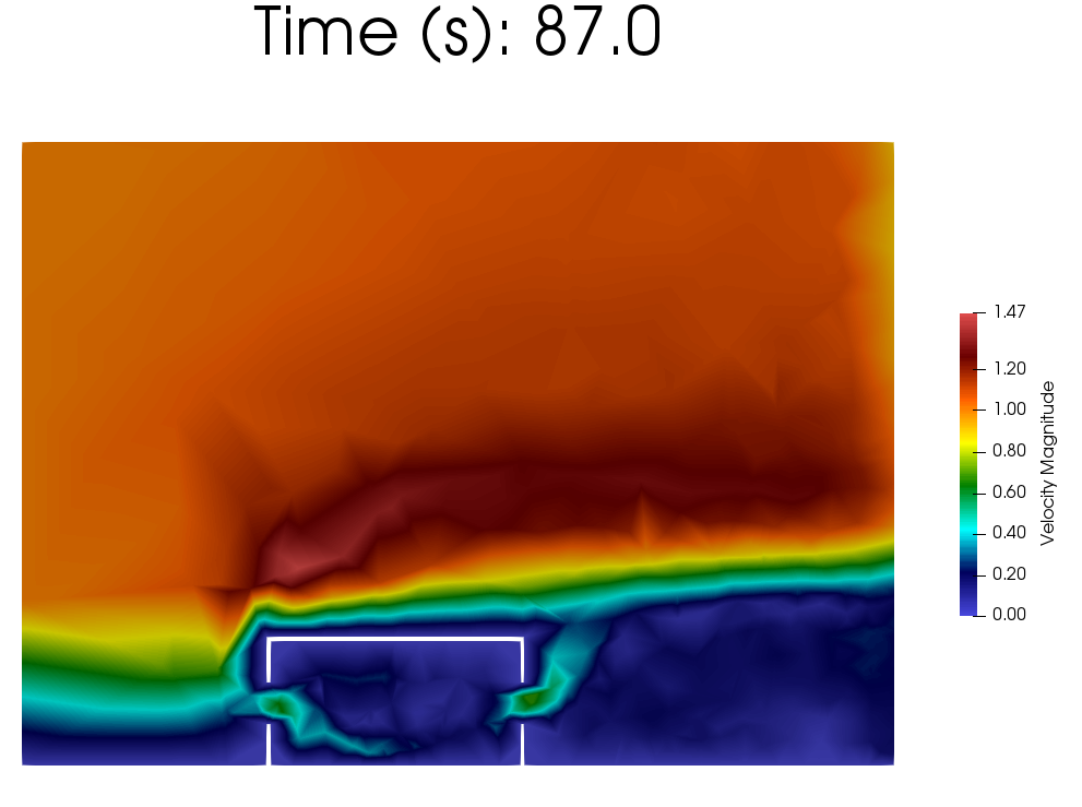
8.3 Reference temperature
In Fluidity, the option subtract_out_hydrostatic_level changes the buoyancy term. For the Boussinesq case, it changes to and this option should always be used. Note that, using Boussinesq, the reference density does not influence any of the terms in the momentum equation. It may however influence the outcome of diagnostic fields depending on density. The reference temperature, used in the equation of state, needs to correspond to the ambient temperature. This will avoid unwanted re-circulation near the boundary where the pressure is defined, i.e. at the outlet boundary of the domain in the case presented here. Effect on the pressure field of not using the proper reference temperature is shown in Figure 8.4.
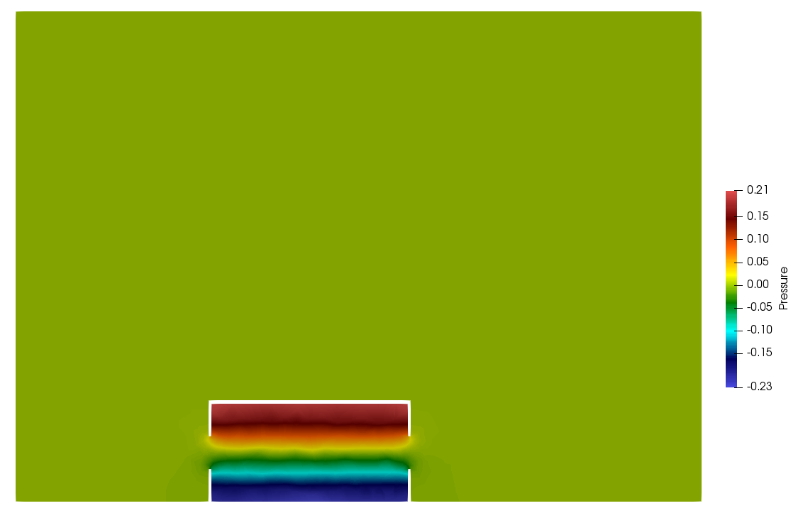
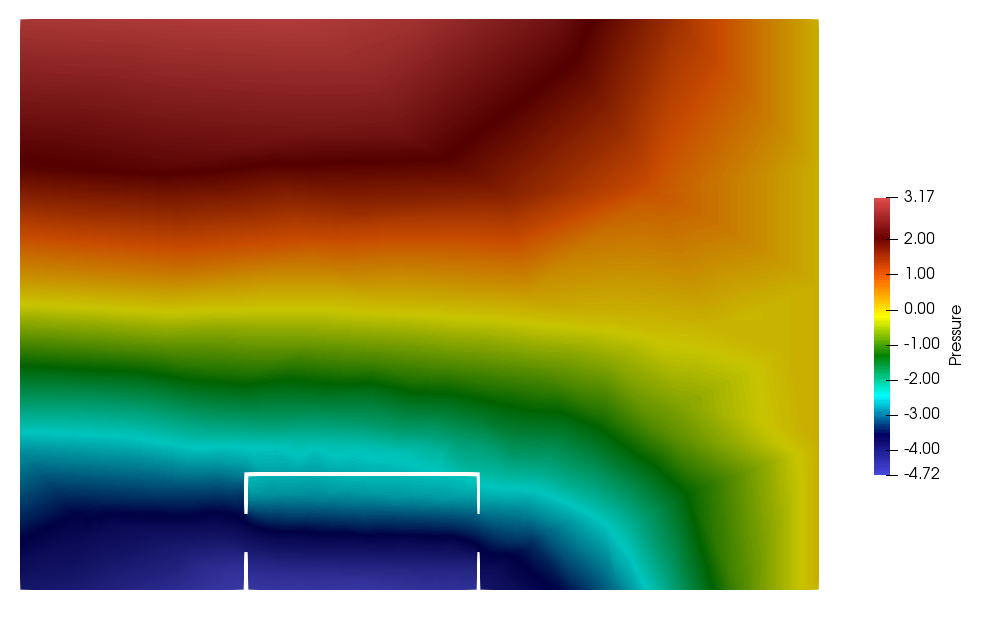
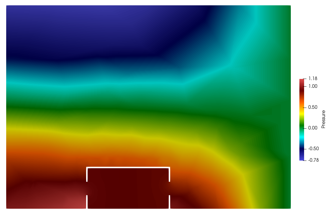
8.4 Walls boundary condition
See Section 4.5.3 for more details.
The velocity boundary conditions on solid surfaces can be applied either weakly or strongly and can represent a slip or a no-slip behaviour.
-
•
It is to be noted that when boundary conditions are applying weakly, the discrete solution will not satisfy the boundary condition exactly. Instead the solution will converge to the correct boundary condition along with the solution in the interior as the mesh is refined. An alternative way of implementing boundary conditions, so called strongly imposed boundary conditions. Although this guarantees that the Dirichlet boundary condition will be satisfied exactly, it does not at all mean that the discrete solution converges to the exact continuous solution more quickly than it would with weakly imposed boundary conditions. Strongly imposed boundary conditions may sometimes be necessary if the boundary condition needs to be imposed strictly for physical reasons. Unlike the strong form of the Dirichlet conditions, weak Dirichlet conditions do not force the solution on the boundary to be point-wise equal to the boundary condition. If boundary conditions are applied weakly, then the following options need to be turned on in Diamond:
-
–
Under Pressure field: spatial_discretisation/continuous_galerkin/
integrate_continuity_by_parts -
–
Under Velocity field: spatial_discretisation/continuous_galerkin/
advection_terms/integrate_advection_by_parts
-
–
-
•
A no-slip boundary condition is defined by the three components of the velocity being equal to zero, while a slip boundary condition corresponds to the normal component of the velocity only being equal to zero. Both are Dirichlet type.
There are two options available to apply a Dirichlet boundary condition in Fluidity:
-
•
align_bc_with_cartesian: the three components of the velocity are assigned - Always work.
-
•
align_bc_with_surface: the normal and the two tangential components of the velocity are assigned - Does not always work.
The option align_bc_with_surface in the Dirichlet type boundary condition is not well-implemented in Fluidity and not always work properly.
In summary:
-
•
The option align_bc_with_cartesian should always be preferred if possible.
-
•
Only one no-slip Dirichlet align_bc_with_surface applied strongly is allowed, while several can be used when applied weakly.
-
•
For a slip boundary condition weakly applied, align_bc_with_cartesian type for simple geometry or no_normal_flow type for any geometry should be used. The Dirichlet align_bc_with_surface type does not work.
-
•
A slip boundary condition is recommended instead of a no-slip one if the boundary layer is not going to be fully resolved with the chosen mesh, to avoid weird behaviour of the temperature field.
8.5 Consistent interpolation
This section is almost a copy-paste of the Fluidity manual [1], section 7.6 and the user can refer to it for more details. Unless you are running a simulation with discontinuous Galerkin fields, the option consistent_interpolation needs to be enabled in any prognostic and diagnostic field. Indeed, the application of adaptive re-meshing divides naturally into three sub-problems. The first is to decide what mesh is desired; the second is to actually generate that mesh. The third, discussed here, is how to interpolate any necessary data from the previous mesh to the adapted one. For the third problem, the consistent_interpolation is almost universally used. This standard method consists of evaluating the previous solution at the locations of the nodes in the adapted mesh. The choice should be consistent_interpolation, unless any of the following conditions hold:
-
•
The simulation has a discontinuous prognostic field which must be interpolated.
-
•
Conservation of some field is crucial for the dynamics.
-
•
The field is obtained using a time averaged algorithm in Fluidity.
In such cases, galerkin_projection should be applied. In the case of time averaged fields that will avoid excessive numerical diffusion.
8.6 Comparing files
Files, like *.flml files, can be compared using the Command 1:
meld is not a Fluidity tool and needs to be installed if not already using the command:
8.7 Checkpointing
When running a Fluidity simulation, checkpoint files are outputted every period, where is specified by the user under io_checkpointing (see Figure 7.3). Checkpoints are useful if a simulation needs to be restarted from a particular point in time.
The files needed to checkpoint at a certain time step (index) are the following:
-
•
The flml checkpoint file: name_index_checkpoint.flml
-
•
The CoordinateMesh msh file: name_CoordinateMesh_index_checkpoint.msh
-
•
The PressureMesh vtu file: name_PressureMesh_index_checkpoint.vtu
-
•
The VelocityMesh vtu file: name_VelocityMesh_index_checkpoint.vtu
It must be noted that if the simulation is run on parallel on processors there will be CoordinateMesh msh and halo files as well as folders with the PressureMesh and VelocityMesh vtu files on top of the pvtu files.
The new simulation will then be running using the command:
It should be repeated that there is currently a bug in Fluidity concerning the time-average field: when a simulation is run from a checkpoint the value of the previous time-average is not properly read from the checkpointed files implying that the average is then not correct. This will later be fixed but for now it is recommended to the user to specify a spin-up time higher than the checkpoint time to start a new time-average.
Chapter 9 Fluidity in parallel
9.1 When should Fluidity be run in parallel ?
As a rule of thumb, there should be 50,000 nodes per processor. If the number of nodes per processor is smaller than that, there will be no benefit in switching from serial to parallel, although the simulation should still run in parallel.
9.2 Running on a PC
In order for a simulation to run in parallel, the mesh first needs to be decomposed using flredecomp (more information on this tool is found in [1]). A mesh is decomposed (from 1 to 4 parts for example) using Command 1. It must be noted that the number of processors used to run the mpiexec command needs to be equal to the maximum number of parts in either the original or new mesh. If a mesh was to be recomposed from 4 parts to 1, the Command 2 is the one to use. Once the mesh is decomposed the simulation can be run in parallel, on 4 processors for example, using Command 3.
Note: The tool fldecomp in Fluidity is obsolete and the tool flredecomp has always to be used.
9.3 Running on CX1
Fluidity can also be run on a computer cluster, and here the example of Imperial cluster CX1 is detailed. More information on CX1 in general is available online, particularly regarding job sizing:
- •
- •
The following singlenode.pbs script shown in Code 1 will run a simulation with the pre-installed Fluidity version on the chosen single node queue.
Apart from the normal CX1 procedure, it is worth noting the loading of the pre-installed Fluidity modules with module load ese-software and module load ese-fluidity. During and after the simulation, the output can be visualised directly in the ephemeral directory. A maximum wall time in the flml can also be specified to match the one in the pbs file to ensure the simulation will be terminated on a checkpoint.
If a multinode queue is to be used, the mesh needs to be decomposed in the total number of processors used (i.e. for CX1: number of cpus number of nodes).
Chapter 10 Post-processing data obtained with Fluidity
10.1 ParaView
Simulation’s results can be viewed by loading the vtu files into ParaView. This software can be downloaded from https://www.paraview.org/, where a number of useful information can also be found, such as guides and tutorials. The interface is shown in Figure 10.1 and a number of useful features are described below:
-
•
Slice: a type of view that allows the user to view an orthogonal slice of the simulation’s results.
-
•
Glyph: a type of filter that shows the data at specific points as markers with an orientation and size defined by the input. Typically, this tool is used to display velocity vectors.
-
•
Probe: a type of filter that gives the values of the fields at a specific location.
-
•
Surface with edge: a type of render that shows the values of a field as well as the mesh used during the simulation.
-
•
Follow cullback: is found in Backface styling and allows the user to tune the rendering of the front and back faces (with regards to the camera), modifying the visualisation.
It is then recommended to play around with all ParaView features to become familiar with them.
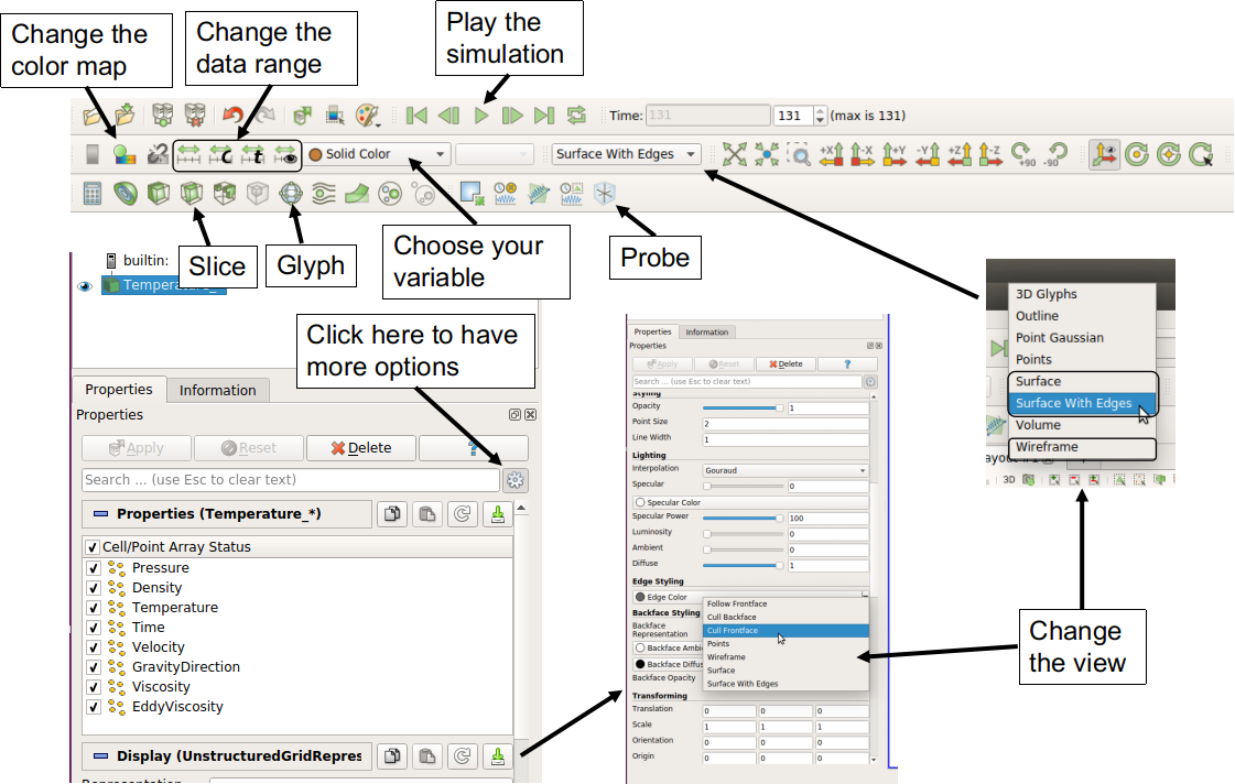
10.2 Python scripts
The results can also be visualised and analysed using python scripts. The main python library used is the library vtk. In addition, the vtktools.py and vtutools.py python modules can also be used and imported in every script. vtktools.py and vtutools.py can be found in <<FluiditySourcePath>> under /python/ and /python/fluidity/ diagnostics/, respectively. Both are including in the materials attached to this manual. Both scripts are really useful to work, manipulate and post-process *.vtu or *.pvtu data. Lots of example of python script using the vtk library can also be found online:
-
•
https://www.vtk.org/doc/nightly/html/pages.html: the sections Class to Examples and Class to Tests are plenty of python and C++ script examples.
-
•
https://lorensen.github.io/VTKExamples/site/Python/ is also full of script using vtk functions.
Documentations for vtk can also be found online:
-
•
version 5.10 https://www.vtk.org/doc/release/5.10/html/index.html
-
•
version 7.1 https://www.vtk.org/doc/release/7.1/html/
To take advantage of all the new vtk features, it is recommended to download one of the latest release available online: https://www.vtk.org/ and install it following https://www.vtk.org/Wiki/VTK/Configure_and_Build. During the installation, in the Cmake interface, use the ‘advanced mode’ (t keyboard) and make sure that VTK WRAP PYTHON is set to ON. Note that installing the vtk library is not trivial and a number of errors can occur. Please ask the help of an advanced user if needed. Once the latest version is installed, the user should use the executable vtkpython located under <<vtkPath>>/bin/. Note that they are lots of major change between versions 5 and 6 of vtk. Please refer to the following for more details:
- •
- •
Note: the probe tool provided in the vtktools.py can behave weirdly when trying to probe data near/on solid walls due to inconsistent behaviour of the vtk library. This weird behaviour might also differ depending the version of vtk you are using. Have a look of the function in vtktools.py to know why and/or ask an advanced user to explain what is happening…
The library matplotlib is the one recommended to plot data. Following are two examples of python scripts using the module vtktools.py, the library vtk and that are inspired by some functions in vtutools.py. The following examples of python script will show how to:
-
•
Compute the mass flow rate at openings: MassFlowRate.py
-
•
Compute the radius of a thermal plume: PlumeRadius.py
10.3 Mass flow rate at the openings
10.3.1 Test case
The script MassFlowRate.py is located in Scripts/MassFlowRate/. The following results and discussions are based on data obtained with example 3dBox_Case11.flml.
10.3.2 Generality and method
Equation
The mass flow rate () through an opening is defined by equation 10.1:
| (10.1) |
where is the density of the fluid, is the magnitude of the normal component of the velocity (normal to the surface considered) and is the surface of the opening.
Method
When calculating the mass flow rate at openings, to compensate the possible lack of mesh resolution, it is recommended to do an average over several planes through the opening’s thickness or (what we think to be less accurate) to compute the mass flow rate over a plane located at the middle of the opening’s thickness, i.e thickness/2. In the script MassFlowRate.py provided the first option is chosen. A Cartesian grid is defined through the opening, data are extracted for each points of this grid, then averaged to obtain the final mass flow rate through that particular plane. This procedure is repeated for several planes along the thickness of the opening. Finally, the final mass flow rate is computed averaging mass flow rates obtained for each planes.
Input variables
The user input variables are the followings:
-
•
path_simu is the path where the simulation is located.
-
•
basename is the name of the simulation.
-
•
vtu_start, vtu_end and vtu_step are respectively the first vtu file, the last vtu file and the step between those vtu files that the user want to consider. This allows the user to have the evolution of the mass flow rate as a function of the time.
-
•
ni_start, ni_end and ni_step, where i stands for the x, y and z direction, define the size of the grids that the user want consider. This allows the user to test different grid resolutions.
10.3.3 Results
The mass flow rate is evaluated at the two openings of the box. Zone1 refers to the opening on the left, i.e. the one closer to the inlet of the domain where the velocity is prescribed, while Zone2 refers to the opening on the right, i.e. closer to the outlet of the domain where the pressure is prescribed. In that particular case, the thickness of the openings is towards the x-direction, therefore the -component of the velocity is used. The Cartesian grids where the data are extracted are aligned with . Figure 10.2 shows the computed mass flow rate at the inlet and at the outlet of the box as a function of time for a grid resolution . Playing around with the script, the user will notice that for low grid resolution, the computed mass flow rate at the inlet is not equal to the one at the outlet. Increasing the resolution of the grid, the input and output mass flow rate tends to be more equal to each other, which is expected. Also, increasing the grid resolution tends to converge to the correct mass flow rate but at some point continuing increasing the grid resolution does not improve results. It is also to mention that the computed mass flow rate at the inlet and at the outlet are not strictly equal, due to lack of mesh resolution, and tends to be equal while refining the mesh at the openings.

The results are written in the text file MassFlowRate.txt where the 7 columns corresponds to:
-
1.
Resolution used in the direction
-
2.
Resolution used in the direction
-
3.
Resolution used in the direction
-
4.
Time in seconds
-
5.
Mass flow rate at the inlet of the box in
-
6.
Mass flow rate at the outlet of the box in
-
7.
Error in percentage (%) between the inlet and outlet mass flow rates
10.3.4 Numerical implementation
The results described above are implemented in a python script and the main libraries used are the followings:
10.4 Plume radius
10.4.1 Test case
The script PlumeRadius.py is located in the folder Scripts/PlumeRadius. The script can be tested using the file Case9b_Box_300.vtu (obtained from 3dBox_Case9b.flml) located in the same folder. However, in the following, pictures and plots showing results were obtained using another set of more complicated simulations not provided with this manual. Indeed, in the case presented below, the box is in the middle of the big domain with two openings at the bottom, two openings at the top and a heat source at the bottom of the box. Moreover, if the user wants to use that script then the path (path of where the data are stored), the name (name of the simulation) and the vtu_start (the number of the vtu) need to be changed in the script according to the user’s requirements. Also note that the data presented below is obtained from instantaneous data. In practice, the user should have included the time average of the velocity (and of any other interesting quantities) in the simulation and those quantities should be used to compute the time average radius of the plume. In that case, the line Vz=up.GetField(’Velocity’)[:,2] should be replaced by Vz=up.GetField(’VelocityAverage’)[:,2], assuming that VelocityAverage is the name of the time average velocity field chosen by the user in Diamond.
10.4.2 Generality
The radius of the plume is usually defined by equation 10.2:
| (10.2) |
where is the time-averaged maximum velocity and is a threshold usually equal to 0.02. In the following, it is assumed that the -axis is pointing up. Therefore, the maximum velocity is given by the -component of the velocity, i.e .
The Figure 10.3 summarises the different methods tested to compute the radius of the plume as a function of the height. All these methods are described in detail in the following sections.

10.4.3 Description of the methods
a) Algorithms
The general idea is to get the geometry of the plume at different height and deduce the radius of the plume based on the geometry. Based on equation 10.2, two methods are tested and described in the following sections:
-
•
Method I: Based on the global maximum velocity:
-
•
Method II: Based on the local maximum velocity:
Method I based on the global velocity
This method consists of generating a contour based on the global maximum velocity and then creating slice cuts at every height.


Method II based on the local velocity
This method consists of generating slices at every height, then determining the local maximum velocity and finally generating the contour of the plume.


Comparison of the two methods
Figure 10.6 shows the plume’s contour at different height generated by Algorithm 1 and Algorithm 2. The red lines are the results obtained for Algorithm 1, while black lines are the results obtained using Algorithm 2.
It can be noted that Algorithm 1 generally predicts a geometry of smaller area than the one found with Algorithm 2 (as also shown in Figure 10.6).


b) Cleaning the geometry - Step 6 of the algorithms
The process of cleaning the geometry is explained below:
-
•
The polygons within the main plume geometry are deleted. In Figure 10.7(a), for example, the polygons within the main polygon are not taken into account in the later computation of the radius. However, the area of these polygons is kept (see section 2.3.1 - method 1b to know why and have more details).
- •
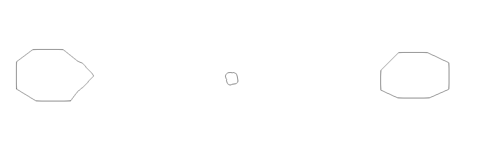
c) Radius of the plume - Step 7 of the algorithms
The computation of the radius is performed based on two different methods described in the following sections:
-
•
Method 1: the radius is computed based on the area of the polygons.
-
•
Method 2: the radius is computed based on the distance between the center and the exterior boundary of the polygons.
Method 1 based on the area
This method consists of computing the radius of the plume assuming an ideal circle, such that:
| (10.3) |
where is the total area of the plume. The aim of this method is to compute and then determine the radius of the plume based on equation 10.3. This method is explained based on Figure 10.8 geometry. Figure 10.8 shows the 2D geometry of the plume at a certain height . The geometry is composed by 3 main polygons (labelled 1, 2 and 3). The polygon 1 has also another polygon (labelled 4) within. Based on the cleaning process described in the previous paragraph, the small polygon 4 is detected. The total area is therefore computed in two different ways as follows:
-
•
Method 1a - polygon 4 is ignored.
(10.4) -
•
Method 1b - polygon 4 is taken into account and subtracted to the total area.
(10.5)
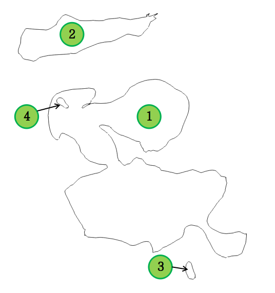
Method 2 based on the distance
In this section, the radius is computed based on the distance between a centre point of the plume and the nodes defining the exterior boundaries of the polygons (themselves defining the plume geometry) and denoted by pink dots in Figure 10.9. A simple arithmetic mean is performed:
| (10.6) |
where is the distance between the node and the centre of the plume and is the total number of nodes defining the polygons.
Now the main question consists of determining the centre of the plume. For this, two approaches are tested:
-
•
Method 2a: the centre of the plume is assumed to be the centre of the source.
-
•
Method 2b: the centre of the plume is taken locally at each height. For this, the centroid of the polygons defining the plume geometry is used as the local centre.
It has to be noted that this method is somehow not really accurate for the following reason:
- •
-
•
For both case shown in Figure 10.9, it can be observed that certain region has lot of point defining the boundary (it happens where there is sharp change in the geometry) while other regions have less nodes. Once again, the computed radius will be artificially weighted by the region where there are lots of nodes, which is not desirable.
However, comparing this method with the one using the area, the mean radii generated are quite close.
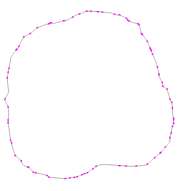
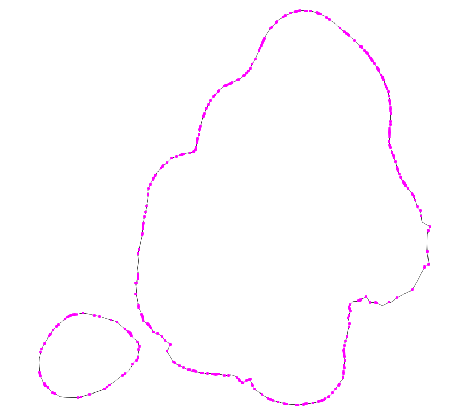
10.4.4 Outputs and plots
Summary of the methods
In summary, these methods give as output:
-
•
Method I.1.a based on the global velocity using the area of the polygons.
-
•
Method I.1.b based on the global velocity using the area of the polygons minus the area of the polygons deleted.
-
•
Method I.2.a based on the global velocity using the distance between the centre of the source and the boundaries of the polygons.
-
•
Method I.2.b based on the global velocity using the distance between the local centre and the boundaries of the polygons.
-
•
Method II.1.a based on the local velocity using the area of the polygons.
-
•
Method II.1.b based on the local velocity using the area of the polygons minus the area of the polygons deleted.
-
•
Method II.2.a based on the local velocity using the distance between the centre of the source and the boundaries of the polygons.
-
•
Method II.2.b based on the local velocity using the distance between the local centre and the boundaries of the polygons.
Text files with data
The data are written in text files and each files are explained below.
-
•
Radius_Global.txt
Radii computed by method I - Global Velocity - 5 columns-
1.
The height in meters
-
2.
computed by method I.2.a
-
3.
computed by method I.2.b
-
4.
computed by method I.1.a
-
5.
computed by method I.1.b
-
1.
-
•
Radius_Local.txt
Radii computed by method II - Local Velocity - 5 columns-
1.
The height in meters
-
2.
computed by method II.2.a
-
3.
computed by method II.2.b
-
4.
computed by method II.1.a
-
5.
computed by method II.1.b
-
1.
-
•
Centre_Global.txt
Centre of the plume computed by method I - Global Velocity - 5 columns-
1.
The height in meters
-
2.
coordinate of the local centre computed by method I.2.b
-
3.
coordinate of the local centre computed by method I.2.b
-
4.
coordinate of the source
-
5.
coordinate of the source
Note that columns 4 and 5 have constant values.
-
1.
-
•
Centre_Local.txt
Centre of the plume computed by method II - Local Velocity - 5 columns-
1.
The height in meters
-
2.
coordinate of the local centre computed by method II.2.b
-
3.
coordinate of the local centre computed by method II.2.b
-
4.
coordinate of the source
-
5.
coordinate of the source
Note that columns 4 and 5 have constant values.
-
1.
-
•
Location_VelocityZ_max.txt
Location of the velocity max in the domain - 6 columns-
1.
coordinate of the location of the maximum velocity for method II
-
2.
coordinate of the location of the maximum velocity for method II
-
3.
coordinate of the location of the maximum velocity for method II
-
4.
coordinate of the location of the maximum velocity for method I
-
5.
coordinate of the location of the maximum velocity for method I
-
6.
coordinate of the location of the maximum velocity for method I
Note that columns 4, 5 and 6 have constant values.
-
1.
Plots
This section shows examples of plots that can be obtained. Figure 10.10 shows the variation of the plume’s radius as a function of the height for all the methods presented above. Figure 10.11(a) shows the variation of the maximum velocity as a function of the height for methods I and II. Figure 10.11(b) shows the location of the plume centre as a function of the height for methods I and II. The green lines are for method I, while the blue lines are for method II. In Figure 10.11(b), the black crosses depicts the location of the maximum velocity while using method II. The global maximum velocity is depicted by black diamonds. Figure 10.12 to Figure 10.15 show the and locations of the plume centre as a function of the height for the method I.2 and II.2. The error bars depicts the radius computed by the associated method centred on the source location (Figure 10.12 and Figure 10.13) and the local plume’s centre (Figure 10.14 and Figure 10.15).
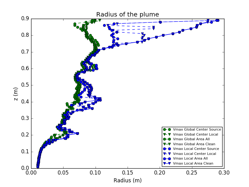
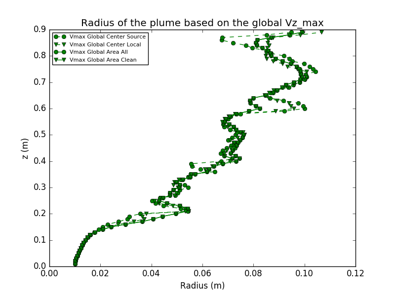

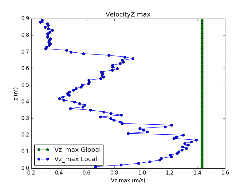
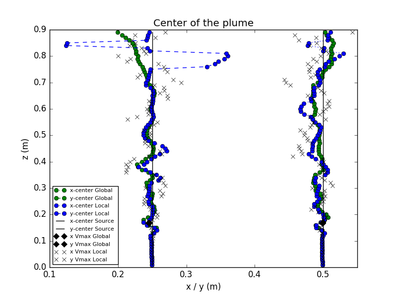

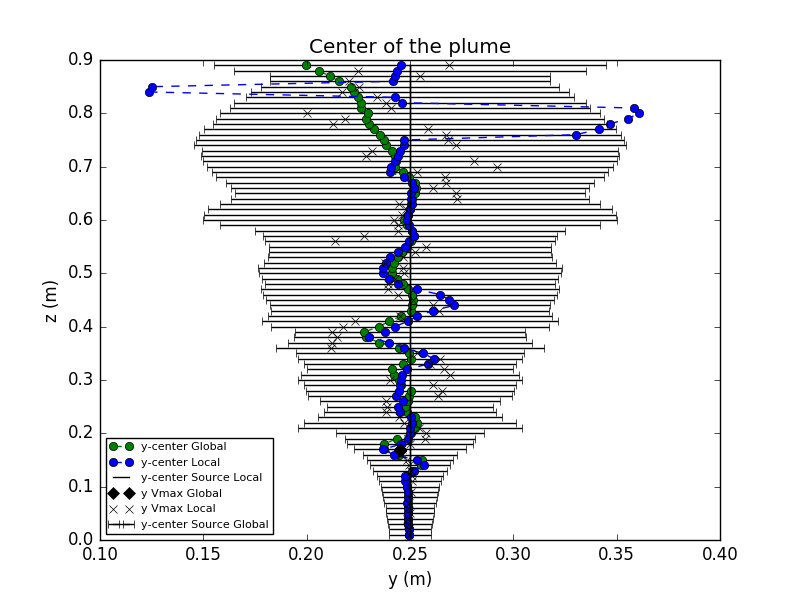

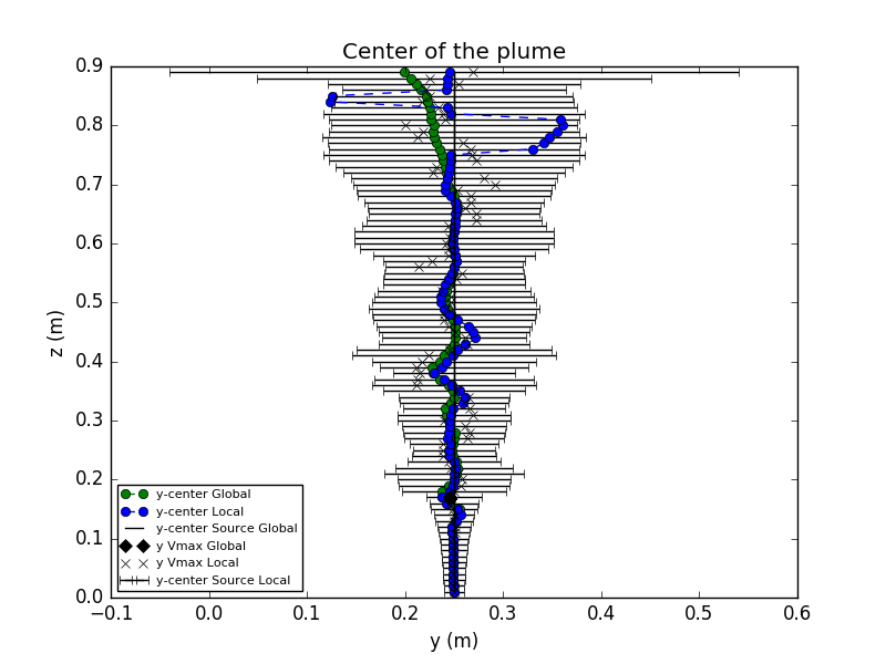
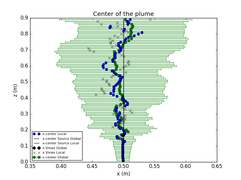
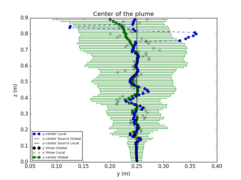


10.4.5 Numerical implementation
All the methods described above are implemented in a python script and the main libraries used are:
- •
-
•
shapely is used to play around with the geometry. For example, the centroid of the polygons and the detection of polygons within others are done using this library.
- •
10.5 *.stat file
While a Fluidity simulation is running, a *.stat file is generated, which is basically a text file that can be viewed with any text editor. This file records a number of interesting information such as the number of nodes, the maximum and minimum values of each fields… As shown in Figure 10.16, information in the *.stat file can also be viewed directly using the graphical interface statplot launched by typing in a terminal:
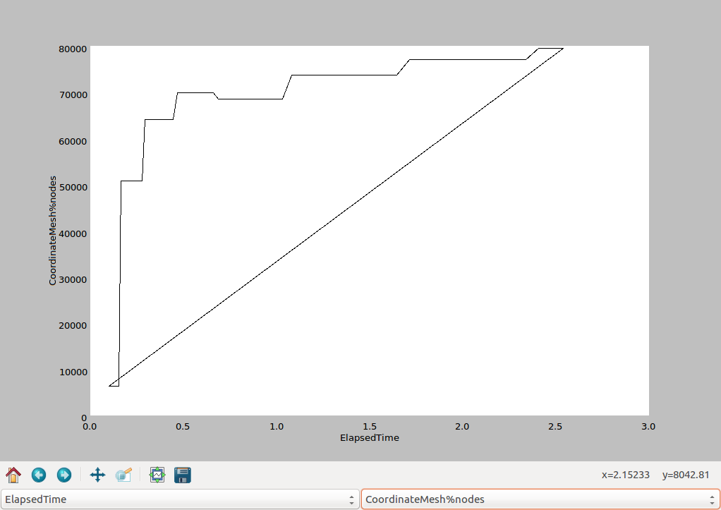

The data can also be read easily using a python script: an example of python script, StatReader.py, can be found in the folder Scripts/StatReader/. As shown in Code 7, Line 10, the fluidity_tools library is required. The *.stat file needs to be imported (Line 25 in Code 7), then the data can be extracted (see Lines 32 to 38 in Code 7). This allows the manipulation of the data and some plots are shown in Figure 10.17


10.6 fltools
A number of Fluidity tools exist and are detailed in the manual. Here are described the more useful ones. For information, the executable of these tools are located under the directory: <<FluiditySourcePath>>/bin/.
10.6.1 rename_checkpoint
When running a simulation from a checkpoint, the new simulation will have the name of the simulation following by _checkpoint and the files’ numbering will re-start at 0. Therefore, it can be useful to rename these files afterwards to visualise them as continuous files in ParaView for example. Hence, the tool rename_checkpoint allows to rename the ParaView files (*.vtu or *.pvtu) of a simulation that has been checkpointed. It is run typing in a terminal Command 2, where base_filename is the original name of the simulation before it was checkpointed and index is the index at which it was checkpointed. For example, if simulations were run from a file called Case11_Box_10_checkpoint.flml the resulting checkpointed files would have to be renamed with the command rename_checkpoint Case11_Box 10.
10.6.2 pvtu2vtu
When running a simulation in parallel, *.pvtu files are generated. When visualising these files in ParaView and particularly when using the cull frontface visualisation style, the overlapping region used during parallelisation (due to the domain decomposition) are visible, making difficult to view the results. One easy way to avoid this is to convert the *.pvtu files into *.vtu files using the tool pvtu2vtu which combines the *.pvtu obtained in parallel into *.vtu files. This tool is run typing in a terminal Command 3, where base_filename is the name of the simulation, index and last index are the first and the last index of the files to convert.
10.6.3 genpvd
Finally, genpvd can be used to generate a *.pvd file from the list of *.vtu or *.pvtu files. This will notably allow the user to have access to the simulation real time. It can be run using Command 4, where base_filename is the name of the simulation. It must be noted that checkpointed files will have to be renamed before this can be done.
Chapter 11 Others
11.1 Past and present people using Fluidity
Following are past and present people working with Fluidity to perform outdoor simulations and/or indoor-outdoor exchange simulations. This manual was initiated by Dr Laetitia Mottet, post-doc in the Earth Science and Engineering department, Imperial College London and in the Architecture department, University of Cambridge; and Carolanne Vouriot, PhD student in the Civil Engineering department, Imperial College London. It is also important to mention that Fluidity was initially developed by Prof. Christopher Pain c.pain@imperial.ac.uk, department of Earth Science and Engineering, Imperial College London.
| Complex outdoor simulations | ||||
|---|---|---|---|---|
| Since 2000 | E. Aristodemou | Senior Lecturer | London South Bank University | |
| Since 2016 | L. Mottet | Post-doc | Imperial / Cambridge | |
| Since 2017 | H. Woordward | Post-doc | Imperial | |
| Box simulations of indoor - outdoor exchanges | ||||
| Summer 2017 | Faron Hesse | MRes | ICL | H. Burridge |
| Summer 2017 | Jean-Etienne Debay | Intern | Cam | M. Davies Wykes |
| Since 2018 | Carolanne Vouriot | PhD Student | ICL | H. Burridge |
| Summer 2018 | Nouhaila Fadhi | Intern | Cam | M. Davies Wykes |
| Summer 2018 | Theresa Bischof | MSc | ICL | H. Burridge |
| Summer 2018 | Sam Charlwood | UROP | Cam | M. Davies Wykes |
Contacts: prioritise people in red if you have any questions or amendment to this manual to suggest.
-
•
Elsa Aristodemou - aristode@lsbu.ac.uk
-
•
Laetitia Mottet - l.mottet@imperial.ac.uk
-
•
Henry Burridge - h.burridge@imperial.ac.uk
-
•
Megan Davies Wykes - msd38@cam.ac.uk
-
•
Huw Woodward - h.woodward@imperial.ac.uk
-
•
Carolanne Vouriot - carolanne.vouriot12@imperial.ac.uk
11.2 Online open-source data set
Following is a non-exhaustive list of open-source experimental and/or numerical data available for indoor-outdoor exchange and urban environment simulations.
- •
-
•
Indoor-outdoor exchanges
-
–
Please contact Laetitia Mottet and/or Carolanne Vouriot if you are aware of open-source data available online, either numerical or experimental, on indoor-outdoor exchanges.
-
–
Bibliography
- [1] AMCG. Fluidity manual (Version 4.1). Imperial College London, April 2015.
- [2] Christophe Geuzaine and Jean-Francois Remacle. Gmsh: a three-dimensional finite element mesh generator with built-in pre- and post-processing facilities. International Journal for Numerical Methods in Engineering, 2009.
- [3] C.C. Pain, A.P. Umpleby, C.R.E. De Oliveira, and A.J.H. Goddard. Tetrahedral mesh optimisation and adaptivity for steady-state and transient finite element calculations. Computer Methods in Applied Mechanics and Engineering, 190:3771–3796, 2001.
- [4] E. Aristodemou, T. Bentham, C. Pain, and A. Robins. A comparison of mesh-adaptive les with wind tunnel data for flow past buildings: mean flows and velocity fluctuations. Atmospheric Environment journal, 43:6238–6253, 2009.
- [5] D. Pavlidis, G. J. Gorman, J. L. M. A. Goms, C. C. Painr, and H. ApSimon. Synthetic-eddy method for urban atmospheric flow modelling. Boundary-Layer Meteorology, 136:285–299, 2010.
- [6] E. Aristodemou, L.M. Boganegra, L. Mottet, D. Pavlidis, A. Constantinou, C.C. Pain, A. Robins, and H. ApSimon. How tall buildings affect turbulent air flows and dispersion of pollution within a neighbourhood. Environmental Pollution, 233:782–796, 2018.
- [7] J. Franke, A. Hellsten, H. Schlünzen, and B. Carissimo. Best practice guideline for the CFD simulation of flows in the urban environment, COST Action 732. COST Office, 2007.