Gravitational production of sterile neutrinos

Fotis Koutroulis¹, Oleg Lebedev², Stefan Pokorski¹

¹Institute of Theoretical Physics, Faculty of Physics, University of Warsaw,
ul. Pasteura 5, 02-093 Warsaw, Poland
²Department of Physics and Helsinki Institute of Physics,
Gustaf Hällströmin katu 2a, FI-00014 Helsinki, Finland

Abstract

We consider gravitational production of singlet fermions such as sterile neutrinos during and after inflation. The production efficiency due to classical gravity is suppressed by the fermion mass. Quantum gravitational effects, on the other hand, are expected to break conformal invariance of the fermion sector by the Planck scale–suppressed operators irrespective of the mass. We find that such operators are very efficient in fermion production immediately after inflation, generating a significant background of stable or long-lived feebly interacting particles. This applies, in particular, to sterile neutrinos which can constitute cold non–thermal dark matter for a wide range of masses, including the keV scale.

1 Introduction

The existence of right-handed neutrinos $\nu_{R}$ is motivated by the small but non-zero masses of the active neutrinos [1, 2, 3, 4, 5, 6]. In addition to generating masses, $\nu_{R}$ can be relevant to the problem of dark matter (DM). Indeed, light (mostly) right-handed neutrinos, which we will also call ‘‘sterile’’ neutrinos, can have a lifetime longer than the age of the Universe and also have the properties characteristic of dark matter, e.g. very weak interactions with the Standard Model (SM) states. This makes $\nu_{R}$ an attractive minimalistic dark matter candidate [7, 8, 9], as reviewed in [10, 11].

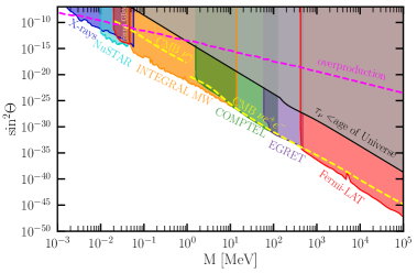
Figure 1: Constraints on the active-sterile neutrino mixing angle $\Theta$ from astrophysics and cosmology. The figure is from Ref. [15].

It is natural to assume that there are 3 right-handed neutrinos, although there could be many more of them [12]. The two heavier $\nu_{R}$ would then be responsible for the active neutrino masses, while the lightest one can play the role of dark matter [13, 14]. This is possible if the sterile-active mixing angle is tiny, which makes the lightest $\nu_{R}$ long lived. The cosmological and astrophysical constraints on this angle are shown in Fig. 1 (see [16] for further details). The most important processes are the decays $\nu_{R}\rightarrow\nu_{a}\gamma$ and $\nu_{R}\rightarrow\nu_{a}e^{-}e^{+}$, where $\nu_{a}$ is the active neutrino. These lead to the X-ray and gamma ray emission as well as to the CMB distortion, which set significant constraints on decaying neutrinos.

If the mixing angle is not too small, sterile neutrinos are produced by the Standard Model thermal bath via the Dodelson-Widrow mechanism [7]. In principle, this could generate the right amount of ‘‘warm’’ dark matter, although this possibility is now disfavored [17, 18, 19, 20, 21, 22, 23]. The corresponding constraint is shown in the figure by the ‘‘overproduction’’ line. In particular, substantial mixing angles are ruled by overabundance of dark matter.

The thermal production mechanism assumes that the initial abundance of sterile neutrinos is zero. We show that this assumption is not quite realistic [24] since particles are produced during and after inflation via gravitational effects. In particular, Planck-suppressed operators induced by quantum gravity play an important role during the inflaton oscillation epoch [25] and can readily dominate production of light fermions. The characteristic particle energy is far below the Standard Model bath temperature which makes such fermions good cold dark matter candidates, in contrast to the particles produced via the thermal emission.

In general, gravitational particle production creates a significant background of dark relics, which affects the predictions of most non-thermal dark matter models [24]. Hence, predictive models require either excellent control over quantum-gravity induced operators or a mechanism for dilution of gravitationally produced particles. An example of the latter is provided by models with an extended period of matter domination resulting in a low reheating temperature [26].

In what follows, we study gravitational fermion production during inflation and in the inflaton oscillation epoch. In these periods, the energy density and the field values are the largest, leading to most efficient particle production.

2 Fermion production during inflation

Generally, particles are produced due to the expansion of the Universe [27, 28, 29], which can be attributed to the change in the vacuum state in a time-dependent background (see [30] for a review). In what follows, we study in detail fermion production in the Friedmann Universe [31]. For our exposition to be self-contained, we start with a pedagogical introduction following Ref. [32].

Consider a Dirac fermion $\Psi$ of mass $M$ which has negligible couplings to other fields. The corresponding results for a Majorana fermion can be obtained by a simple rescaling. We assume the fermion to be light enough relative to the Hubble rate during inflation, $M\ll H$, so that there is no ‘‘energetic’’ obstacle to its production. Since the Friedmann metric is conformally flat and the fermion action is conformally invariant apart from the mass term, particle production via classical gravity is fully controlled by the fermion mass $M$. In what follows, we verify this explicitly and compute the resulting abundance of $\Psi$.

2.1 Basics

The starting point is the Dirac equation in curved space,

$$(i\gamma^{\alpha}\nabla_{\alpha}-M)\,\Psi=0\;,$$ (1)

which follows from the action $\int d^{4}x\sqrt{|g|}\bar{\Psi}(i\gamma^{\alpha}\nabla_{\alpha}-M)\,\Psi$, where $g_{\mu\nu}$ is the space-time metric, $\nabla$ is the covariant derivative and $\alpha$ is the local Lorentz index. The Friedmann metric in terms of the conformal time $x_{0}\equiv\eta$ reads

$$ds^{2}=a(x_{0})^{2}\,\eta_{\mu\nu}dx^{\mu}dx^{\nu}\;.$$ (2)

Using the Weyl transformation

$$g_{\mu\nu}=\Omega^{2}\tilde{g}_{\mu\nu}~{},~{}\Psi=\Omega^{-3/2}\tilde{\Psi}~{},~{}e_{\alpha}^{\mu}=\Omega^{-1}\tilde{e}_{\alpha}^{\mu}~{},$$ (3)

where $\Omega=a(x_{0})$ and $e_{\alpha}^{\mu}$ is the vierbein, the factor $a(x_{0})$ can be eliminated from the action apart from the mass term. Dropping the tilde over the transformed quantities, the resulting Dirac equation reads

$$(i\gamma^{\mu}\partial_{\mu}-a(\eta)M)\,\Psi=0\;,$$ (4)

which is the flat space Dirac equation with a time-dependent mass. The latter causes particle production.

The above equation can be solved as follows. The solution space is spanned by the orthonormal basis $\{U,V\}$, where the basis vectors characterized by the 3-momentum ${\bf k}$ and the spin projection $s$ have the form

$$U_{{\bf k},s}(\eta,{\bf x})={e^{i{\bf k}\cdot{\bf x}}\over(2\pi)^{3/2}}\left(\begin{matrix}u_{A,k}(\eta)\\ s\,u_{B,k}(\eta)\end{matrix}\right)\otimes h_{s}({\bf\hat{k}})\;,$$ (5)

where $k\equiv|{\bf k}|$, ${\bf\hat{k}}={\bf k}/|{\bf k}|$, $h_{s}$ are the helicity 2-spinors satisfying

$${\bf\hat{k}}\cdot\vec{\sigma}\;h_{s}=s\,h_{s}~{}~{},~{}~{}s=\pm 1\;,$$ (6)

and $\vec{\sigma}$ are the sigma matrices. $u_{A,B}$ are complex functions of time to be determined, depending on $a(\eta)$. In spherical coordinates, ${\bf\hat{k}}=(\theta,\phi)$ and

$${\bf\hat{k}}\cdot\vec{\sigma}=\left(\begin{matrix}\cos\theta&e^{-i\phi}\,\sin\theta\\ e^{i\phi}\,\sin\theta&-\cos\theta\end{matrix}\right)~{},~{}h_{-1}=\left(\begin{matrix}e^{-i\phi}\,\sin{\theta\over 2}\\ -\cos{\theta\over 2}\end{matrix}\right)~{},~{}h_{1}=\left(\begin{matrix}e^{-i\phi}\,\cos{\theta\over 2}\\ \sin{\theta\over 2}\end{matrix}\right)\;.$$ (7)

In this convention, $-i\sigma^{2}h_{s}^{*}({\bf\hat{k}})=-se^{i\phi}h_{-s}({\bf\hat{k}})$ and $h_{s}(-{\bf\hat{k}})=-h_{-s}({\bf\hat{k}})$.

The $V$-vectors can be chosen as $V_{i}=-i\gamma^{2}U_{i}^{*}$, so that

$$V_{{\bf k},s}(\eta,{\bf x})=-{e^{-i{\bf k}\cdot{\bf x}}\over(2\pi)^{3/2}}\left(\begin{matrix}-u_{B,k}^{*}(\eta)\\ s\,u_{A,k}^{*}(\eta)\end{matrix}\right)\otimes h_{s}(-{\bf\hat{k}})\,e^{i\phi}\;,$$ (8)

in the convention

$$\gamma^{0}=\left(\begin{matrix}I&0\\ 0&-I\end{matrix}\right)~{},~{}\gamma^{i}=\left(\begin{matrix}0&\sigma^{i}\\ -\sigma^{i}&0\end{matrix}\right)~{}.$$ (9)

Since

$$h^{\dagger}_{s}({\bf\hat{k}})\,h_{r}({\bf\hat{k}})=\delta_{rs}\;,$$ (10)

the orthonormality of the basis,

$$(U_{i},U_{j})=\delta_{ij}~{},~{}(U_{i},V_{j})=0\;,$$ (11)

requires

$$|u_{A}|^{2}+|u_{B}|^{2}=1\;.$$ (12)

Here the scalar product is meant in the usual sense, $(f,g)=\int d^{3}x\,f^{\dagger}g$, and following [30], we take index $i$ to be continuous. In particular, the spacial part of the wave functions is described by the orthonormal set ${e^{i{\bf k}\cdot{\bf x}}\over(2\pi)^{3/2}}$.

Using the above Ansatz, the equation of motion (EOM) reduces to

$$i\partial_{\eta}\left(\begin{matrix}u_{A}\\ u_{B}\end{matrix}\right)=\left(\begin{matrix}aM&k\\ k&-aM\end{matrix}\right)\;\left(\begin{matrix}u_{A}\\ u_{B}\end{matrix}\right)~{}.~{}$$ (13)

This implies, in particular, that the $u_{A,B}$ normalization (12) is time-independent. Note that the evolution in the $(u_{A},u_{B})$ space is unitary, i.e. SU(2). Denoting the time derivative $\partial_{\eta}$ by a prime, we reduce the system to second order differential equations,

$$u_{A}^{\prime\prime}+(iMa^{\prime}+a^{2}M^{2}+k^{2})\,u_{A}=0\,$$ (14)

$$u_{B}^{\prime\prime}+(-iMa^{\prime}+a^{2}M^{2}+k^{2})\,u_{B}=0\,,$$ (15)

where $k$ is the magnitude of the 3-momentum. The solutions must have certain asymptotic behaviour corresponding to the $in$ or $out$ vacuum. In particular, during inflation the solutions are Hankel functions of $\eta$.

In the Heisenberg picture, the field operator is expressed via creation/annihilation operators times the basis functions solving the Dirac equation,

$$\Psi(x)=\sum_{i}\left(a_{i}U_{i}+b_{i}^{\dagger}V_{i}\right)\;.$$ (16)

Here the operators satisfy the usual time-independent anti-commutation relations, $\{a_{i},a^{\dagger}_{j}\}=\delta_{ij}$, $\{b_{i},b^{\dagger}_{j}\}=\delta_{ij}$, etc. The vacuum is defined by $a_{i}|0\rangle=b_{i}|0\rangle=0$. The Hilbert space is constructed via Fock states by acting with creation operators on the vacuum.

The creation/annihilation operators are attached to a specific solution basis. Since the basis is complete at a given $\eta$, a new set of basis functions can be expressed as

$$\tilde{U}_{i}=\sum_{j}\left(\alpha_{ij}U_{j}+\beta_{ij}V_{j}\right)~{}~{},~{}~{}\tilde{V}_{i}=\sum_{j}\left(\alpha_{ij}^{*}V_{j}+\beta_{ij}^{*}U_{j}\right)\;.$$ (17)

where the second relation follows from the first one. Using orthonormality of the basis, one has

$$\beta_{ij}=(V_{j},\tilde{U}_{i})~{}~{},~{}~{}\alpha_{ij}=(U_{j},\tilde{U}_{i})\;.$$ (18)

The new basis is also orthonormal, which together with

$$\Psi=\sum_{i}\left(a_{i}U_{i}+b_{i}^{\dagger}V_{i}\right)=\sum_{i}\left(\tilde{a}_{i}\tilde{U}_{i}+\tilde{b}_{i}^{\dagger}\tilde{V}_{i}\right)\;,$$ (19)

implies

$$\tilde{a}_{i}=\sum_{j}\left(\alpha^{*}_{ij}a_{j}+\beta^{*}_{ij}b^{\dagger}_{j}\right)\;,$$ (20)

such that

$$\langle\tilde{N}_{i}\rangle\equiv\langle 0|\tilde{a}_{i}^{\dagger}\tilde{a}_{i}|0\rangle=\sum_{j}|\beta_{ij}|^{2}\;.$$ (21)

This gives the mean number of $tilded$ particles of type $i$ in the original vacuum $|0\rangle$ defined by the absence of any un-tilded particles.

Now let us consider a particular set of basis transformations which affects $u_{A,B}$ while leaving the spin and spacial components of the wave functions intact, i.e. preserves the Ansatz (5). Since $\{U,V\}$ is a complete basis, the $U$-vectors transform as

$$\tilde{U}_{{\bf k},s}=\alpha_{{\bf k},s}U_{{\bf k},s}+\beta_{{\bf k},s}V_{-{\bf k},s}$$ (22)

under the basis change by virtue of (18). Here we use a shorthand notation for the indices of $\alpha$ and $\beta$: $ij\rightarrow{{\bf k},s}$ since there is only one term in the sum. Employing the explicit parametrization of $\tilde{U},\tilde{V}$ as in (5) and computing various scalar products, one finds

$$\beta_{{\bf k},s}={\rm phase}\times(u_{A,k}\tilde{u}_{B,k}-u_{B,k}\tilde{u}_{A,k})\;,$$ (23)

where the (time-independent) phase factor is irrelevant for our purposes. Here we have used the fact $u_{A,B}$ depend only on the magnitude of the 3-momentum as is clear from (15).

The EOM (13) imply that $\beta$ is time-independent,

$$\beta^{\prime}=0\;,$$ (24)

which can also be viewed as conservation of the cross product of 2 vectors under SU(2) rotations. This conservation law is important since it allows for evaluation of $\beta$ at any convenient point in time.

2.2 Particle number calculation

The number of particles produced by inflation is given by $|\beta|^{2}$ for the 2 bases corresponding to the $in$ and $out$ states, respectively. The physical picture is as follows: we define the system initially in the $in$ state ($\eta\rightarrow-\infty$) with no particles, while the observed particle number is measured with respect to the $out$ vacuum ($\eta\rightarrow\infty$), as given by (21) in the Heisenberg picture. Eq. 13 implies that, far in the past, the system is Minkowskian since $a\rightarrow 0$ and only the $k$ terms matter. In the future, it is also Minkowskian: $a\rightarrow\infty$ but $H\rightarrow 0$, which makes the system effectively static, while the momentum terms can be neglected. Hence the $in$ and $out$ vacua are those of flat space. As usual, the mode functions are the positive frequency $\omega$ modes, $e^{-i\omega\eta}$, or more precisely,

$$\left(\begin{matrix}u_{A}\\ u_{B}\end{matrix}\right)\propto e^{-i\int\omega(\eta)d\eta}$$ (25)

with $\omega>0$. This fixes the $in$ and $out$ boundary conditions in the asymptotic regions.

Naturally, the result depends on $a(\eta)$, in particular, whether inflation is followed by a radiation-dominated or a matter-dominated expansion period. We consider both possibilities in what follows.

2.2.1 Inflation followed by radiation domination

The function $a(\eta)$ is chosen such that it describes a smooth transition from inflation at early times to radiation domination at late times [32],

$$a(\eta)=\left\{\left({1\over a_{e}H_{e}}-\eta\right)^{-1}H_{e}^{-1}~{}~{}{\rm for}~{}~{}\eta\leq 0~{}~{},~{}~{}a^{2}_{e}H_{e}\left(\eta+{1\over a_{e}H_{e}}\right)~{}~{}{\rm for}~{}\eta>0\right\}~{},$$ (26)

$$H(\eta)=\left\{H_{e}~{}~{}{\rm for}~{}~{}\eta\leq 0~{}~{},~{}~{}H_{e}\,(a_{e}/a)^{2}~{}~{}{\rm for}~{}~{}\eta>0\right\}~{},$$ (27)

where $a_{e}$ and $H_{e}$ are the scale factor and the Hubble rate at the end of inflation, respectively. Note that $H(\eta)=a^{\prime}/a^{2}$ in terms of the conformal time.

At $\eta\rightarrow-\infty$, the $aM$ terms in (13) can be neglected and the positive eigenstate of the matrix on the right hand side (RHS) is $(1/\sqrt{2},1/\sqrt{2})^{T}$. Hence the positive frequency solution is

$$\left(\begin{matrix}u_{A}\\ u_{B}\end{matrix}\right)\overset{\small{\eta\rightarrow-\infty}}{\longrightarrow}\left(\begin{matrix}{1/\sqrt{2}}\\ {1/\sqrt{2}}\end{matrix}\right)\;e^{-ik\eta}\;.$$ (28)

This fixes uniquely the $in$ solution in the inflationary regime.

At $\eta\rightarrow\infty$, the matrix is diagonal and the positive eigenvalue solution corresponds to

$$\left(\begin{matrix}u_{A}\\ u_{B}\end{matrix}\right)\overset{\small{\eta\rightarrow\infty}}{\longrightarrow}\left(\begin{matrix}1\\ 0\end{matrix}\right)\;e^{-i\int\omega(\eta)d\eta}\;,$$ (29)

with $\omega\rightarrow a(\eta)M$. This fixes uniquely the $out$ solution in the radiation domination regime.

In what follows, we construct analytical solutions for $u_{A},u_{B}$ away from $\eta\sim 0$. In this case, $a(\eta)$ can be approximated by $-{1\over H_{e}\eta}$ during inflation and by $a^{2}_{e}H_{e}\eta$ during radiation domination.

Inflationary regime. In the inflationary regime, $u_{A}$ satisfies

$$\eta^{2}u_{A}^{\prime\prime}+\left(k^{2}\eta^{2}+\left[{iM\over H_{e}}+{M^{2}\over H_{e}^{2}}\right]\right)\,u_{A}=0\;.$$ (30)

This is the Bessel-type equation, whose solution with the right asymptotics are the Hankel functions. One finds

$$u_{A}(\eta)=\sqrt{\pi k\eta\over 4}\,e^{-i{\pi\over 2}(1-iM/H_{e})}\,H^{(2)}_{{1/2}-{iM/H_{e}}}(k\eta)\;,$$ (31)

assuming $M/H_{e}\ll 1$. Using $H^{(2)}_{\nu}(-z)=-e^{i\nu\pi}H_{\nu}^{(1)}(z)$ and $\sqrt{-1}=-i$ according to the phase convention of the Hankel argument, one can rewrite it as

$$u_{A}^{in}(a)=\sqrt{\pi k\over 4aH_{e}}\,e^{i{\pi\over 2}(1-iM/H_{e})}\,H^{(1)}_{{1/2}-{iM/H_{e}}}\left({k\over aH_{e}}\right)\;.$$ (32)

The $u_{B}$ function is obtained by flipping the sign of $M$,

$$u_{B}^{in}(a)=\sqrt{\pi k\over 4aH_{e}}\,e^{i{\pi\over 2}(1+iM/H_{e})}\,H^{(1)}_{{1/2}+{iM/H_{e}}}\left({k\over aH_{e}}\right)\;.$$ (33)

Radiation-dominated regime. The equation for $u_{A}$ is

$$u_{A}^{\prime\prime}+\left(k^{2}+iMa_{e}^{2}H_{e}+\eta^{2}\,M^{2}a_{e}^{4}H_{e}^{2}\right)\,u_{A}=0\;.$$ (34)

The solution is a parabolic cylinder function $D_{\nu}(z)$. Defining

$$C={k^{2}\over 2Ma_{e}^{2}H_{e}}\;,$$ (35)

we find

$$u_{A}^{out}(\eta)=e^{-{\pi\over 4}C}D_{-iC}\left(e^{i\pi/4}\sqrt{2M\over H(\eta)}\right)\times{\rm phase}\;,$$ (36)

where the time-dependent phase is universal for $u_{A}$ and $u_{B}$, and thus irrelevant for our purposes.

The equation for $u_{B}$ is obtained by $M\rightarrow-M$ in (34). The solution vanishing at infinity is

$$u_{B}^{out}(\eta)=\sqrt{C}\,e^{-{\pi\over 4}C+{i\pi\over 4}}D_{-1-iC}\left(e^{i\pi/4}\sqrt{2M\over H(\eta)}\right)\times{\rm phase}\;,$$ (37)

where the ‘‘phase’’ is the same as that in $u_{A}$. The solution approaches zero as $1/\eta$.

We note that (29) does not fix the normalization of $u_{B}$ since it vanishes at infinity. To determine the normalization factor, one needs to make the asymptotic behaviour of the positive frequency mode more precise by including the $k/aM$ correction to the eigenstate of the matrix in (13),

$$\left(\begin{matrix}u_{A}\\ u_{B}\end{matrix}\right)\overset{\small{\eta\rightarrow\infty}}{\longrightarrow}\left(\begin{matrix}1\\ {k\over 2aM}\end{matrix}\right)\;e^{-i\int\omega(\eta)d\eta}\;,$$ (38)

while the correction to $\omega$ can be neglected. This shows that $u_{B}$ vanishes as $1/\eta$ and also fixes the normalization as in (37).

Particle production. We have obtained the solutions which are valid in two regimes: the $in$ solution works during inflation and the $out$ solution works only in the radiation-dominated regime. At the end of inflation $a\sim a_{e}$, corresponding to the transition region, both of them are approximately valid. Since $\beta$ is time-independent for the exact solutions, we can compute $\beta$ at this point. The validity of this approximation is supported by numerical analysis.

The average particle number with momentum $k$ is computed via

$$|\beta_{{\bf k},s}|^{2}=|u_{A,k}^{in}u_{B,k}^{out}-u_{B,k}^{in}u_{A,k}^{out}|^{2}\;,$$ (39)

and the total particle number density is [30]

$$n=\int{d^{3}{\bf k}\over(2\pi)^{3}a^{3}}\,|\beta_{{\bf k},s}|^{2}\;.$$ (40)

Given the analytical results, one can compute $\beta_{k}(a_{e})$ numerically for different $k$. One finds that for $M\ll H_{e}$, the $in$ solutions at $a\sim a_{e}$ approximately retain their asymptotic form, while the $out$ solutions can change drastically. The main factor determining $\beta_{k}(a_{e})$ is the value of $C$:

$$C\ll 1\Rightarrow|\beta_{k}|^{2}\sim 1/2\;,$$ (41)

$$C\gg 1\Rightarrow|\beta_{k}|^{2}\sim 0\;,$$ (42)

so $C\sim 1$ corresponds to the cut-off of particle production and 3-momenta above $a_{e}\sqrt{H_{e}M}$ are not generated. The $|\beta_{k}|^{2}$ fall-off with $k$ is fast, $\propto k^{-6}$ at large $k$, hence these modes do not contribute to the integral in any significant way.

This qualitative behavior can be understood analytically. The $in$ state does not change significantly from $a\sim 0$ to $a_{e}$ independently of the momenta as long as $M\ll H_{e}$, so

$$\left(\begin{matrix}u_{A}\\ u_{B}\end{matrix}\right)^{in}(a_{e})\sim\left(\begin{matrix}1/\sqrt{2}\\ 1/\sqrt{2}\end{matrix}\right)\times{\rm phase}\;,$$ (43)

where the overall phase is irrelevant for our purposes. For the out state, the zero argument limit of the $D$-functions, i.e. $H_{e}\gg M$, gives

$$\left(\begin{matrix}u_{A}\\ u_{B}\end{matrix}\right)^{out}(a_{e})\sim\left(\begin{matrix}e^{-\pi C/4}\sqrt{\cosh{\pi C\over 2}}\\ e^{-\pi C/4}\sqrt{\sinh{\pi C\over 2}}\end{matrix}\right)\times{\rm phase}\;.$$ (44)

This explains why $C$ acts as the main driver of particle production efficiency: for $C\gg 1$, the $in$ and $out$ states coincide up to the phase and $\beta\sim 0$. For small $C$, only $u_{A}$ is significant for the $out$ state, so $\beta\sim 1/\sqrt{2}$.

Relic abundance. We observe that the momentum cutoff corresponds to $C\sim 1$ so that production of particles with momenta larger than [32]

$$k_{*}=a_{e}\sqrt{H_{e}M}$$ (45)

is suppressed. To understand the physics of this cut-off, define $a_{M}$ as the moment when the Hubble rate equals the particle mass,

$$a_{M}:~{}~{}H(a_{M})=M\;.$$ (46)

Since $H=H_{e}(a_{e}/a)^{2}$,

$$k_{*}=a_{M}\,M\;.$$ (47)

Therefore, only particles with physical 3-momenta $k/a<M$ at the time $H=M$ are created. In other words, these particles are non-relativistic or, at best, semi-relativistic.

Inserting the step function $\theta(k_{*}-k)$ in the integral (40), we get [32]

$$n(a)\sim 4\times{1\over 2\pi^{2}}\times{1\over 2}\,{M^{3}\over 3}\,\left({a_{M}\over a}\right)^{3}\;,$$ (48)

where 4 comes from the d.o.f. of the Dirac field and $1/2$ from $|\beta_{k}|^{2}$ of the excited momentum modes. This formula implies that particle production stops when $H=M$ and after that the total particle number is conserved. The density is proportional to the conformal symmetry breaking parameter $M$ and consistent with thermal interpretation of the de Sitter space: indeed $n\sim M^{3}$ is expected at $T\sim H_{M}=M$.

The above result conforms to our expectations: massless particles (or highly relativistic ones) are not produced at all since the system becomes scale-invariant in this case. Note also that production of superheavy particles, $M>H_{\rm infl}$, would be suppressed, although this is not immediately clear in our approximation $M\ll H_{e}$ in the Hankel functions.

The abundance $Y$ of created particles can be estimated at $a=a_{M}$, after which it remains constant. It is defined by

$$Y={n\over s_{\rm SM}}~{}~{},~{}~{}s_{\rm SM}={2\pi^{2}\over 45}\,g_{*}T^{3}\;,$$ (49)

where $s_{\rm SM}$ is the entropy density of the SM thermal bath at temperature $T$ and $g_{*}$ is the effective number of degrees of freedom contributing to the entropy.

Radiation domination after inflation can correspond either to inflaton oscillations in a $\phi^{4}$ potential followed by reheating or instant reheating in an arbitrary potential, both of which lead to the same scaling $a(\eta)$ and the same relic abundance of $\Psi$. The reheating temperature $T_{R}$ is found via

$$3H_{R}^{2}M_{\rm Pl}^{2}={g_{*}(T_{R})\pi^{2}\over 30}\,T_{R}^{4}\;,$$ (50)

and $H_{e}/H_{R}=(a_{R}/a_{e})^{2}$. Since $a_{R}/a_{M}=(M/H_{R})^{1/2}$ and $s_{\rm SM}(a_{M})=(a_{R}/a_{M})^{3}\,s_{\rm SM}(a_{R})$, we have

$$Y\simeq 4.5\times 10^{-3}\;\left({M\over M_{\rm Pl}}\right)^{3/2}\;,$$ (51)

with no dependence on the Hubble rate (!) nor reheating temperature as long as $M\ll H_{e}$. The observational constraint on dark matter

$$Y\leq 4.4\times 10^{-10}\;{{\rm GeV}\over M}\;$$ (52)

then requires

$$M\lesssim 2\times 10^{8}\,{\rm GeV}\;,$$ (53)

if the fermion $\Psi$ is $stable$ or very long-lived. This is independent of the Hubble rate during inflation as long as it is larger than the fermion mass, which we find quite remarkable. The above result implies that the abundance of lighter fermions ($M\ll 10^{8}$ GeV) is negligible and there are no useful constraints.

Here we assume that $\Psi$ is Dirac, while for the Majorana fermion the abundance should be divided by 2 to account for two Majorana d.o.f.

One may imagine that the fermion with mass $2\times 10^{8}\,{\rm GeV}$ produced by gravity during inflation constitutes all of the dark matter. However, its density perturbations are not correlated with that of the inflaton, hence it is disfavored by isocurvature constraints.

2.2.2 Inflation followed by matter domination

It is possible that inflation is followed by a long period of matter domination. This is the case when the inflaton oscillations occur in a $\phi^{2}$ potential and the inflaton decays very slowly. Particle production takes place in that period so that the $out$ boundary conditions on the wave function should be imposed during the matter domination era. Although this possibility appears to be less common in the literature, we find it equally viable.

The Hubble rate scales as $a^{-3/2}$, therefore solving $a^{\prime}/a^{2}=H_{e}(a_{e}/a)^{3/2}$ with the boundary condition at $a_{e}$ corresponding to $\eta=0$, we get

$$H=H_{e}\left({a_{e}\over a}\right)^{3/2}~{}~{},~{}~{}a={1\over 4}a_{e}^{3}H_{e}^{2}\left(\eta+{2\over a_{e}H_{e}}\right)^{2}\;.$$ (54)

At $\eta\gg 1/(a_{e}H_{e})$, the EOM for $u_{A}$ reads

$$u_{A}^{\prime\prime}+\left({i\over 2}MH_{e}^{2}a_{e}^{3}\,\eta+{1\over 16}M^{2}H_{e}^{4}a_{e}^{6}\,\eta^{4}+k^{2}\right)\,u_{A}=0\;,$$ (55)

while the EOM for $u_{B}$ is obtained by the replacement $M\rightarrow-M$. The oscillation frequency squared is now a quartic polynomial in time and the exact solution is challenging to find. Hence, we solve the equation numerically. The oscillation frequency at late times is $\omega\simeq aM={1\over 4}MH_{e}^{2}a_{e}^{3}\,\eta^{2}$ such that the boundary condition at $\eta\rightarrow\infty$ becomes

$$\left(\begin{matrix}u_{A}\\ u_{B}\end{matrix}\right)^{out}\simeq\left(\begin{matrix}1\\ {2k\over MH_{e}^{2}a_{e}^{3}\,\eta^{2}}\end{matrix}\right)\times e^{-{i\over 12}MH_{e}^{2}a_{e}^{3}\,\eta^{3}}\;.$$ (56)

Using the inflationary $in$ states as before, we then compute $\beta_{k}^{2}$ at $\eta\sim 0$ finding that the effective momentum cut-off for particle production is

$$k_{*}\sim M^{1/3}H_{e}^{2/3}a_{e}\;,$$ (57)

corresponding to $k_{*}=a_{M}M$ as before.

This result can be understood qualitatively from the EOM. As one goes from large $\eta$ to its smaller values for negligible $k\rightarrow 0$, the vector $(1,0)^{T}$ remains an eigenvector of the frequency matrix. So, $u_{B}$ stays close to zero and $\beta_{k}$ takes on its near-maximal value $\sim 1/\sqrt{2}$. As one increases $k$, the $(u_{A},u_{B})^{T}$ vector starts to rotate. The $k^{2}$ term becomes significant in the EOM when $M^{2}H_{e}^{4}a_{e}^{6}\,\eta^{4}\sim k^{2}$. If the damping term is also substantial at this time, the magnitude of $u_{A}$ decreases and that of $u_{B}$ increases due to the constraint $|u_{A}|^{2}+|u_{B}|^{2}=1$. So, the transition to a different regime occurs when all the three terms in $\omega^{2}$ become equally important,

$$MH_{e}^{2}a_{e}^{3}\,\eta\sim M^{2}H_{e}^{4}a_{e}^{6}\,\eta^{4}\sim k^{2}\;,$$ (58)

which gives the above value of $k_{*}$.

Relic abundance The result (48) applies also in the matter dominated case, although the expression for $a_{M}$ changes. It implies that particle production stops at $H\sim M$, as before. Our matter domination assumption means that reheating occurs after particle production terminates,

$$H_{M}=M>H_{R}\;.$$ (59)

The relic abundance is computed at reheating, after which it remains constant. $n(a_{R})$ is obtained from (48) using the scaling $\left({a_{M}\over a_{R}}\right)^{3}={\rm const}\times{T_{R}^{4}\over M^{2}M_{\rm Pl}^{2}}\;,$ where the const depends on the number of d.o.f. One then finds for a Dirac fermion,

$$Y=8\times 10^{-3}\;{M\,T_{R}\over M_{\rm Pl}^{2}}\;,$$ (60)

where $g_{*}\sim 107$ has been assumed. This is smaller than the radiation dominated result (51) due to the constraint $M>H_{R}$, which implies $(M/M_{\rm Pl})^{1/2}>1.8\,T_{R}/M_{\rm Pl}$. For a Majorana fermion, the above $Y$ is to be divided by two.

Requiring the abundance of the fermion to be below that of dark matter, we get the constraint

$$M\lesssim 5\times 10^{14}\,\sqrt{{\rm GeV}\over T_{R}}\;{\rm GeV}\;,$$ (61)

which is weaker than the corresponding radiation domination bound. Combining it with the constraint $M>H_{R}$, one finds that $T_{R}$ must be below $10^{13}$ GeV for the above analysis to apply. The limiting value of $T_{R}$ yields (53).

We find therefore that, in the matter dominated case, the bounds on the abundance and the fermion mass are weaker than those in the radiation domination scenario.

Our conclusion is that sterile neutrino production during inflation is insignificant unless it is very heavy, $M\sim 10^{8}\,$GeV. We next consider fermion production is the postinflationary era.

3 Fermion production in the inflaton oscillation epoch

After inflation completes, the inflaton field starts oscillating around its local minimum. This creates a classical time-dependent background which naturally leads to particle production. Such particle production takes place even in the absence of direct renormalizable couplings between the inflaton and other fields. Indeed, gravity, both classical and quantum, induces gauge invariant Planck–suppressed operators among various fields. Since the inflaton field value as well as the energy scale of the system after inflation is below the Planck scale, one may use the effective field theory (EFT) approach and expand the Lagrangian in terms of operators of increasing dimension. The leading Planck-suppressed operator containing the inflaton $\phi$ and the fermion $\Psi$ has dimension 5,

$${{\cal C}\over M_{\rm Pl}}\,\phi^{2}\,\bar{\Psi}\Psi\;,$$ (62)

where ${\cal C}$ is a dimensionless Wilson coefficient. To be conservative, here we assume approximate $\phi\rightarrow-\phi$ symmetry such that operators with odd powers of $\phi$, e.g. $\phi\bar{\Psi}\Psi$, can be omitted. We also assume conserved parity which forbids the coupling $\phi^{2}\bar{\Psi}\gamma_{5}\Psi$, although this would not bring additional non-trivial effects.

The value of ${\cal C}$ is a free parameter in the EFT description and can only be computed given a complete quantum gravity theory. In particular, it can be calculated in string theory via an $n$-point function, where higher dimensional operators play an important role in phenomenology [33]. Generally, such couplings have a very different structure compared to those generated by graviton exchange [34, 35], e.g. they are not related to the energy-momentum tensor nor to lower order couplings such as $\phi\bar{\Psi}\Psi$.

It is important to note that the above operator is not conformally invariant. Quantum gravity effects generally break conformal invariance as manifested by the existence of the Planck scale itself. Classical gravity also breaks this symmetry, while the breaking is proportional to the fermion mass $M$. In particular, the above operator is induced classically by the oscillating scale factor after inflation [36, 37] with ${\cal C}\propto M$. However, at the quantum gravity level, there is no relation between $M$ and ${\cal C}$.

The operator at hand cannot be suppressed by requiring inflaton shift invariance, which is often invoked during inflation. At small field values around the minimum of the inflaton potential, this symmetry is completely broken. We find no general arguments which would lead to natural suppression of ${\cal C}$. In what follows, we will treat ${\cal C}$ as a free parameter bounded roughly by one, in order for the EFT description to apply.

At dimension 6, there is an additional operator

$${C_{6}\over M_{\rm Pl}^{2}}\,\,\phi^{2}\;\bar{\Psi}i{\not{\nabla\mkern 8.0mu}\mkern-8.0mu}{}\Psi,$$ (63)

which reduces to the above operator on-shell, $i{\not{\nabla\mkern 8.0mu}\mkern-8.0mu}{}\Psi=M\Psi$, such that ${\cal C}=C_{6}\,{M\over M_{\rm Pl}}$. Therefore, we will not consider it separately. Finally, an operator of the form $\phi\partial_{\mu}\phi\,\bar{\Psi}\gamma^{\mu}\Psi$ does not bring anything new since it is a total derivative as long as the vector current is conserved.

3.1 Fermion production rate

During preheating, we can expand the oscillating inflaton field as

$$\phi^{2}(t)=\sum_{n=-\infty}^{\infty}\zeta_{n}e^{-in\omega t}\;,$$ (64)

where $\omega$ is the oscillation frequency and the coefficients $\zeta_{n}$ are $slow$ functions of time. An oscillating background generally entails particle production.

The amplitude ${\cal M}$ for the Dirac fermion-antifermion pair production from the ‘‘vacuum’’ due to the dim-5 operator is

$$-i\int_{-\infty}^{\infty}dt\langle f|V(t)|i\rangle=-i\,{{\cal C}\over M_{\rm Pl}}\,(2\pi)^{4}\delta({\bf{p}}+{\bf{q}})\sum_{n=1}^{\infty}\zeta_{n}\,\delta(E_{p}+E_{q}-n\omega)\;\bar{u}v\;,$$ (65)

where $V(t)$ is the interaction term; $p,q$ are the 4-momenta of the created particles and $u,v$ are the relevant Dirac spinors with given momenta. For a fixed $n$ and neglecting the final state particle masses, we get

$$\sum_{\rm spin}|{\cal M}_{n}|^{2}={{\cal C}^{2}\over M_{\rm Pl}^{2}}\,2(n\,\omega)^{2}\;|\zeta_{n}|^{2}\;.$$ (66)

The reaction rate per unit volume is obtained by integrating over the phase space $\Pi$ and summing the contributions for different $n$,

$$\Gamma=\sum_{n=1}^{\infty}\Gamma_{n}=\sum_{n=1}^{\infty}\int\left(\sum_{\rm spin}|{\cal M}_{n}|^{2}\right)d\Pi={{\cal C}^{2}\over 4\pi M_{\rm Pl}^{2}}\omega^{2}\sum_{n=1}^{\infty}n^{2}\,|\zeta_{n}|^{2}\;.$$ (67)

In the $Majorana$ fermion case, there are two identical particles in the final state. Hence, the correct amplitude can be obtained with 2 different contractions, ${\cal M}_{\rm Maj}=2{\cal M}$. On the other hand, the phase space integral receives the factor of 1/2 due to the identical particles. Thus,

$$\Gamma_{\rm Maj}=2\Gamma={{\cal C}^{2}\over 2\pi M_{\rm Pl}^{2}}\omega^{2}\sum_{n=1}^{\infty}n^{2}\,|\zeta_{n}|^{2}\;.$$ (68)

3.2 Relic abundance

Unless ${\cal C}$ is large, particle production proceeds in a rather mild manner such that backreaction of the produced fermions can be neglected. Then, the particle density for Dirac fermions is found via the Boltzmann equation,

$$\dot{n}+3Hn=2\Gamma\;,$$ (69)

where the dot denotes differentiation with respect to coordinate time $t$ ($ds^{2}=dt^{2}-a(t)^{2}d{\bf x}^{2}$) and the factor of 2 comes from two particles produced in each reaction. The LHS can be written as $a^{-3}{d\over dt}(na^{3})$. To compute the integral, it is convenient to switch to variable $a$, $dt=da/(aH)$, such that

$$n\,a^{3}=\int da\,a^{2}\,{2\Gamma\over H}\;.$$ (70)

At this stage, we need to choose the $local$ inflaton potential. Let us start with the quadratic potential and generalize the result to the quartic potential later. We take

$$V={1\over 2}m_{\phi}^{2}\phi^{2}~{}~{},~{}~{}\phi(t)={\phi_{0}\over a^{3/2}}\,\cos m_{\phi}t\;,$$ (71)

where $\phi_{0}$ is the initial inflaton amplitude at $a=1$. In this case, $\omega=2m_{\phi}\,,\,\zeta_{1}={1\over 4}{\phi_{0}^{2}\over a^{3}}\;.$ Thus, for $Dirac$ fermions,

$$\Gamma={{\cal C}^{2}m_{\phi}^{2}\over 16\pi M_{\rm Pl}^{2}}\;{\phi_{0}^{4}\over a^{6}}\;,$$ (72)

while Hubble rate is

$$H={m_{\phi}\phi_{0}\over{\sqrt{6}}M_{\rm Pl}\,a^{3/2}}\;.$$ (73)

The integral is dominated by the initial moments after inflation and soon thereafter the number density becomes

$$n(t)={{\cal C}^{2}m_{\phi}\over 2\sqrt{6}\pi M_{\rm Pl}}{\phi_{0}^{3}\over a^{3}}\;,$$ (74)

meaning that the total particle number is conserved.

The relic abundance generally depends on how quickly reheating occurs. The matter-dominated (or non-relativistic) expansion period is characterized by

$$\Delta_{\rm NR}=\left({H_{e}\over H_{R}}\right)^{1/2}=a_{R}^{3/4}\;,$$ (75)

where $H_{e}$ and $H_{R}$ are the Hubble rates at the end of inflation and reheating, respectively. Here we have defined $a_{e}=1$ at the end of inflation. $\Delta_{\rm NR}\geq 1$ represents the ‘‘dilution’’ factor: since the produced fermions are relativistic, the matter-dominated expansion period dilutes their energy density. It can also be written as the ratio of the reheating temperature in case of instant reheating over the actual reheating temperature, $\Delta_{\rm NR}\simeq T_{R}^{\rm inst}/T_{R}$.

Solving for $T_{R}$, we find the relic abundance

$$Y=10^{-1}\;{\cal C}^{2}\;{H_{e}^{3/2}\,M_{\rm Pl}^{1/2}\over\Delta_{\rm NR}\,m_{\phi}^{2}}$$ (76)

for $g_{*}=107$, which makes the diluting effect of the matter-dominating era explicit.

3.3 Constraints and implications

It is more convenient to trade $m_{\phi}$ for $\phi_{0}$, which allows us to derive a universal result which is also valid for the quartic inflaton potential. Requiring $Y$ not to exceed that of dark matter, we get

$${\cal C}\lesssim 10^{-4}\;\Delta_{\rm NR}^{1/2}\;{{M_{\rm Pl}^{3/4}}H_{e}^{1/4}\over\phi_{0}}\;\sqrt{{{\rm GeV}\over M}}\;.$$ (77)

This result applies to the quartic inflaton potential $V={1\over 4}\lambda_{\phi}\phi^{4}$ as well. In this case, $\omega\simeq 0.85\sqrt{\lambda_{\phi}}\phi_{0}/a$ and $\zeta_{1}\simeq 0.25\phi_{0}^{2}/a^{2}$, leading to $Y\simeq 1.2\times 10^{-2}\;{\cal C}^{2}\;{\phi_{0}^{2}\over{M_{\rm Pl}^{3/2}}H_{e}^{1/2}}$. Then, the above constraint applies irrespective of the reheating temperature and

$$\Delta_{\rm NR}\simeq 1$$ (78)

in the quartic case. The Dirac and Majorana fermion bounds on ${\cal C}$ are very similar and only differ by a square root of 2.

To understand the strength of the above bound, let us take the typical large-field inflation values $\phi_{0}\sim M_{\rm Pl}$ and $H_{e}\sim 10^{-5}M_{\rm Pl}$. Then,

$${\cal C}\leq 10^{-5}\;\Delta_{\rm NR}^{1/2}\;\sqrt{{{\rm GeV}\over M}}\;.$$ (79)

Therefore, unless the dilution factor is very large, the Wilson coefficient has to be very small, ${\cal C}\ll 1$, for GeV or above GeV scale fermion masses. Otherwise, the Universe would be too dark. The constraint on ${\cal C}$ is weaker than the corresponding bound on the Wilson coefficient of the dim-6 operator $\phi^{4}s^{2}/M_{\rm Pl}^{2}$ for a scalar dark relic $s$ [24], as expected.

This result implies that the constraints on the Wilson coefficients of higher dimensional operators,

$${1\over M^{3}_{\rm Pl}}\phi^{4}\bar{\Psi}\Psi~{},~{}{1\over M^{5}_{\rm Pl}}\phi^{6}\bar{\Psi}\Psi~{},~{}...$$ (80)

are also non-trivial for GeV masses or above. They are weaker roughly by the factor $(M_{\rm Pl}/\phi_{0})^{p}$, where $2p+2$ is the power of the inflaton field in the corresponding operator. As long as $\phi_{0}$ is not far below the Planck scale, the constrains are significant. Therefore, full control over these operators is necessary in order to make reliable predictions.

The fermion–inflaton coupling creates an effective fermion mass during inflation, which may suppress inflationary particle production. For example, if one blindly extrapolates the coupling ${\cal C}\phi^{2}\bar{\Psi}\Psi/M_{\rm Pl}$ to large inflaton field values (where the expansion in $\phi/M_{\rm Pl}$ breaks down), the effective mass would be of order ${\cal C}\phi^{2}/M_{\rm Pl}$. This could be larger than the inflationary Hubble rate $H$, in which case particle production via inflation would be suppressed. This issue is model-dependent and since inflationary particle production is not the leading effect in any case, it is insignificant for our purposes.

An important conclusion we make from the above bound is that the quantum-gravity generated operator $\phi^{2}\bar{\Psi}\Psi/M_{\rm Pl}$ with a small Wilson coefficient can generate all of the dark matter. In particular, keV sterile neutrinos can play the role of dark matter for

$${\cal C}(M\sim{\rm keV})\simeq 10^{-2}\;,$$ (81)

when $\Delta_{\rm NR}\sim 1$. Such neutrinos, and even much lighter ones, would constitute cold dark matter. This can be seen as follows [38]: their initial energy $E_{\Psi}$ is of order $m_{\phi}^{\rm eff}$, which is $m_{\phi}$ for the quadratic and $\sqrt{\lambda_{\phi}}\phi_{0}$ for the quartic inflaton potential. On the other hand, the SM bath temperature $T$ is determined by the scale of the inflaton potential $V^{1/4}(\phi)$. Since

$$E_{\Psi}\sim m_{\phi}^{\rm eff}\ll V^{1/4}\sim T\;$$ (82)

as long as $m_{\phi}\ll\phi_{0}$ and $\lambda_{\phi}\ll 1$, the typical neutrino energy in the relativistic regime is far below the SM bath temperature. In the quadratic case, there is a further suppression factor due to the redshifting of the relativistic neutrino energy relative to $V^{1/4}$. As a result, sterile neutrinos become non-relativistic at $T\gg M$ and thus are ‘‘cold’’ at the stage of structure formation. In contrast, $\nu_{R}$ produced via the Dodelson-Widrow mechanism have the energy related to the temperature of the thermal bath and hence are ‘‘warm’’, which makes this scenario disfavored.

Decaying sterile neutrinos can produce a range of signatures, in particular, monochromatic photons. The latter could fall in the X-ray range as in the Dodelson-Widrow model, although this possibility is not theoretically favored over the others. Heavier decaying neutrinos would lead to diffuse gamma ray emission, which provides us with another avenue to probe sterile neutrino dark matter.

4 Conclusion

We have studied production of feebly interacting fermions, in particular, sterile neutrinos, via gravitational effects during and immediately after high-scale inflation. We find that these effects are important and lead to a background of long-lived or stable relics, which can account for all of the dark matter.

Sterile neutrino production via classical gravity during inflation is suppressed by its mass $M$, which represents a conformal symmetry breaking parameter. If the Universe is dominated by radiation after inflation, the neutrino abundance is given by $Y\sim 10^{-2}\,(M/M_{\rm Pl})^{3/2}$ irrespectively of the inflationary Hubble rate $H\gg M$ and the reheating temperature $T_{R}$. In the case of extended matter domination, the abundance becomes $Y\sim 10^{-2}\,M\,T_{R}/M_{\rm Pl}^{2}$. In either case, the sterile neutrino abundance is negligible unless $M\gtrsim 10^{8}\,$GeV.

After inflation, particles are efficiently produced due to inflaton ($\phi$) oscillations. In order to account for quantum gravity effects, we resort to the EFT description at $\phi<M_{\rm Pl}$ and expand the inflaton-neutrino interactions in inverse powers of $M_{\rm Pl}$, focussing on the lowest order Planck-suppressed operators such as $\phi^{2}\bar{\Psi}\Psi/M_{\rm Pl}$. Since quantum gravity breaks conformal invariance, the Wilson coefficients of these operators are not related to the mass parameter $M$ and we treat them as free parameters. We find that the above operator and its higher dimensional analogs are very efficient in particle production. Even if the corresponding Wilson coefficient is very small, $\phi^{2}\bar{\Psi}\Psi/M_{\rm Pl}$ can readily produce all of the Universe dark matter in the form of long-lived sterile neutrinos. This is the case even for keV scale (or below) sterile neutrinos. The energy of these neutrinos is not related to the temperature of the SM thermal bath $T$, unlike it is in the Dodelson-Widrow mechanism. They become non-relativistic at $T\gg M$ and thus constitute $cold$ dark matter, which is favored by the structure formation constraints.

The gravitational production mechanism is operative irrespective of the active-sterile mixing angle. It creates a background for other sterile neutrino production models such as freeze-in, etc. [40, 41, 42, 43, 44]. If the mixing angle is not too small, one expects to see signatures of decaying dark matter, for instance, monochromatic photons. This possibility remains viable in the X-ray range, as was initially expected in the Dodelson-Widrow model.
 
Acknowledgements. OL acknowledges support by Institut Pascal at Université Paris-Saclay during the Paris-Saclay Astroparticle Symposium 2023, with the support of the P2IO Laboratory of Excellence (program ‘‘Investissements d’aveni’’ ANR-11-IDEX-0003-01 Paris-Saclay and ANR-10-LABX-0038), the P2I axis of the Graduate School of Physics of Université Paris-Saclay, as well as IJCLab, CEA, IAS, OSUPS, and the IN2P3 master project UCMN. The research of S.P. has received partial financial support by the National Science Centre, Poland, grant DEC-2019/35/B/ST2/02008.

References

- [1] P. Minkowski, Phys. Lett. 67B, 421 (1977).
- [2] M. Gell-Mann, P. Ramond and R. Slansky, Conf. Proc. C 790927, 315 (1979) [arXiv:1306.4669 [hep-th]].
- [3] T. Yanagida, Conf. Proc. C 7902131, 95 (1979).
- [4] R. N. Mohapatra and G. Senjanovic, Phys. Rev. Lett. 44, 912 (1980).
- [5] J. Schechter and J. W. F. Valle, Phys. Rev. D 22, 2227 (1980).
- [6] G. Lazarides, Q. Shafi and C. Wetterich, Nucl. Phys. B 181, 287 (1981).
- [7] S. Dodelson and L. M. Widrow, Phys. Rev. Lett. 72, 17-20 (1994).
- [8] X. D. Shi and G. M. Fuller, Phys. Rev. Lett. 82, 2832 (1999).
- [9] K. Abazajian, G. M. Fuller and M. Patel, Phys. Rev. D 64, 023501 (2001).
- [10] A. Boyarsky, O. Ruchayskiy and M. Shaposhnikov, Ann. Rev. Nucl. Part. Sci. 59, 191 (2009).
- [11] A. Boyarsky, M. Drewes, T. Lasserre, S. Mertens and O. Ruchayskiy, Prog. Part. Nucl. Phys. 104, 1-45 (2019).
- [12] W. Buchmuller, K. Hamaguchi, O. Lebedev, S. Ramos-Sanchez and M. Ratz, Phys. Rev. Lett. 99, 021601 (2007).
- [13] T. Asaka, S. Blanchet and M. Shaposhnikov, Phys. Lett. B 631, 151 (2005).
- [14] T. Asaka, M. Laine and M. Shaposhnikov, JHEP 0701, 091 (2007); Erratum: [JHEP 1502, 028 (2015)].
- [15] O. Lebedev and T. Toma, JHEP 05, 108 (2023).
- [16] V. De Romeri, D. Karamitros, O. Lebedev and T. Toma, JHEP 10, 137 (2020).
- [17] A. Boyarsky, A. Neronov, O. Ruchayskiy and M. Shaposhnikov, Mon. Not. Roy. Astron. Soc. 370, 213-218 (2006).
- [18] U. Seljak, A. Makarov, P. McDonald and H. Trac, Phys. Rev. Lett. 97, 191303 (2006).
- [19] A. Boyarsky, A. Neronov, O. Ruchayskiy, M. Shaposhnikov and I. Tkachev, Phys. Rev. Lett. 97, 261302 (2006).
- [20] H. Yuksel, J. F. Beacom and C. R. Watson, Phys. Rev. Lett. 101, 121301 (2008).
- [21] K. Perez, K. C. Y. Ng, J. F. Beacom, C. Hersh, S. Horiuchi and R. Krivonos, Phys. Rev. D 95, no. 12, 123002 (2017).
- [22] M. Ackermann et al. [Fermi-LAT Collaboration], Phys. Rev. D 91, no. 12, 122002 (2015).
- [23] M. Drewes et al., JCAP 1701, 025 (2017).
- [24] O. Lebedev, JCAP 02, 032 (2023).
- [25] O. Lebedev and J. H. Yoon, JCAP 07, no.07, 001 (2022).
- [26] C. Cosme, F. Costa and O. Lebedev, [arXiv:2306.13061 [hep-ph]].
- [27] L. Parker, Phys. Rev. 183, 1057-1068 (1969); A. A. Grib and S. G. Mamaev, Yad. Fiz. 10, 1276-1281 (1969); Y. B. Zeldovich and A. A. Starobinsky, Zh. Eksp. Teor. Fiz. 61, 2161-2175 (1971).
- [28] S. G. Mamaev, V. M. Mostepanenko and A. A. Starobinsky, Zh. Eksp. Teor. Fiz. 70, 1577-1591 (1976); A. A. Grib, S. G. Mamaev and V. M. Mostepanenko, Gen. Rel. Grav. 7, 535-547 (1976); Y. B. Zel’dovich and A. A. Starobinsky, JETP Lett. 26, no.5, 252 (1977).
- [29] D. J. H. Chung, E. W. Kolb and A. Riotto, Phys. Rev. D 59, 023501 (1998); V. Kuzmin and I. Tkachev, Phys. Rev. D 59, 123006 (1999); E. W. Kolb and A. J. Long, Phys. Rev. D 96, no.10, 103540 (2017).
- [30] L. H. Ford, Rept. Prog. Phys. 84, no.11, 116901 (2021).
- [31] L. Parker, Phys. Rev. D 3, 346-356 (1971) [erratum: Phys. Rev. D 3, 2546-2546 (1971)].
- [32] D. J. H. Chung, L. L. Everett, H. Yoo and P. Zhou, Phys. Lett. B 712, 147-154 (2012).
- [33] W. Buchmuller, K. Hamaguchi, O. Lebedev and M. Ratz, Phys. Rev. Lett. 96, 121602 (2006).
- [34] M. Garny, M. Sandora and M. S. Sloth, Phys. Rev. Lett. 116, no.10, 101302 (2016).
- [35] R. T. Co, Y. Mambrini and K. A. Olive, Phys. Rev. D 106, no.7, 075006 (2022).
- [36] Y. Ema, R. Jinno, K. Mukaida and K. Nakayama, JCAP 05, 038 (2015).
- [37] Y. Ema, R. Jinno, K. Mukaida and K. Nakayama, Phys. Rev. D 94, no.6, 063517 (2016).
- [38] O. Lebedev, T. Solomko and J. H. Yoon, JCAP 02, 035 (2023).
- [39] O. Lebedev, Prog. Part. Nucl. Phys. 120, 103881 (2021).
- [40] K. Petraki and A. Kusenko, Phys. Rev. D 77, 065014 (2008).
- [41] A. Merle, V. Niro and D. Schmidt, JCAP 1403, 028 (2014).
- [42] A. Adulpravitchai and M. A. Schmidt, JHEP 1501, 006 (2015).
- [43] M. Drewes and J. U. Kang, JHEP 1605, 051 (2016).
- [44] T. Bringmann, P. F. Depta, M. Hufnagel, J. Kersten, J. T. Ruderman and K. Schmidt-Hoberg, Phys. Rev. D 107, no.7, L071702 (2023).