Neural Collapse in Multi-label Learning with
Pick-all-label Loss

Abstract

We study deep neural networks for the multi-label classification (M-lab) task through the lens of neural collapse (NC). Previous works have been restricted to the multi-class classification setting and discovered a prevalent NC phenomenon comprising of the following properties for the last-layer features: (i) the variability of features within every class collapses to zero, (ii) the set of feature means form an equi-angular tight frame (ETF), and (iii) the last layer classifiers collapse to the feature mean upon some scaling. We generalize the study to multi-label learning, and prove for the first time that a generalized NC phenomenon holds with the “pick-all-label” formulation, which we term as M-lab NC. While the ETF geometry remains consistent for features with a single label, multi-label scenarios introduce a unique combinatorial aspect we term the "tag-wise average" property, where the means of features with multiple labels are the scaled averages of means for single-label instances. Theoretically, under proper assumptions on the features, we establish that the only global optimizer of the pick-all-label cross-entropy loss satisfy the multi-label NC. In practice, we demonstrate that our findings can lead to better test performance with more efficient training techniques for M-lab learning.

1 Introduction

In recent years, deep learning showed tremendous success in classifying problems [28], thanks in part to its ability to extract salient features from data [2]. While the success extends to multi-label (M-lab) classification, the structures of the learned features in the M-lab regime is less well-understood. This work aims to fill this gap by understanding the geometric structures of features for M-lab learned via deep neural networks and utilize the structure for better training and prediction.

Recently, an intriguing phenomenon has been observed in the terminal phase of training overparameterized deep networks for the task of multi-class (M-clf) classification in which the last-layer features and classifiers collapse to simple but elegant mathematical structures: all training inputs are mapped to class-specific points in feature space, and the last-layer classifier converges to the dual of class means of the features while attaining the maximum possible margin with a simplex equiangular tight frame (Simplex ETF) structure [44]. See the top row of Figure 1 for an illustration. This phenomenon, termed Neural Collapse (NC), persists across a variety of different network architectures, datasets, and even the choices of losses [17, 74, 73, 65]. The NC phenomenon has been widely observed and analyzed theoretically [44, 10, 75] in the context of M-clf learning problems. It is applied to understand transfer learning [13, 31], and robustness [44, 23], where the line of study has significantly advanced our understanding of representation structures for M-clf using deep networks.

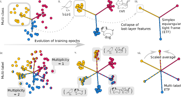
Figure 1: An illustration of neural collapse for M-clf (top row) vs. M-lab (bottom row) learning. For illustrative purposes, we consider a simple setting with the number of classes $K=3$. The individual panels are scatterplots showing the top two singular vectors of the last-layer features $\bm{H}$ at the beginning (left) and end (right) stages of training. The solid (resp. dashed) line segments represent the mean of the multiplicity $=1$ (resp. $=2$) features with the same labels. Panel i-iii. As the training progresses, the last-layer features of samples corresponding a single label, e.g., $\mathtt{bird}$, collapse tightly around its mean. Panel iv-vi. The analogous phenomenon holds in the multi-label setting. Panel iv. A training sample has multiplicity $=1$ (resp. $=2$) if it has one tag (resp. two tags). Panel vi. At the end stage of training, the feature mean of Multiplicity-2 $\{\mathtt{bird},\,\mathtt{cat}\}$ is a scaled tag-wise average of feature means of its associated multiplicity-$1$ samples, i.e., $\{\mathtt{bird}\}$ and $\{\mathtt{cat}\}$.

Our contributions.

We demonstrate a general version of the NC phenomenon in M-lab, and our study provides new insights into prediction and training for the M-lab problem. Specifically, our contributions can be highlighted as follows.

• Multi-label neural collapse phenomenon. We show that the last-layer features and classifier learned via overparameterized deep networks exhibit a more general version of NC which we term it as multi-label neural collapse (M-lab NC). Specifically, while features linked to single-label instances retain a Simplex ETF configuration and undergo collapse, the more complex features with higher label counts intriguingly represent a scaled "tag-wise average" of their single-label counterparts; see the bottom row of Figure 1 for an illustration. This new pattern, referred to as multi-label ETF, is consistently observed in the training of practical neural networks for M-lab tasks.

• Global optimality of M-lab NC. Theoretically, we study the global optimality of M-lab NC based upon a commonly used pick-all-label loss for M-lab learning. By treating the last-layer feature as free optimization variables [10, 75], we show that all global solutions exhibit the properties of M-lab NC with benign global landscape. Moreover, we show that multi-label ETF only requires balanced training samples in each class within the same multiplicity, and allows class imbalanced-ness across different multiplicities.

• M-lab NC guided prediction and training. In practice, we show that our findings lead to improved prediction and training for M-lab learning. For prediction, we propose a new one-nearest-neighbor (ONN) approach: for the given test sample, we assign its label to the tag of the nearest neighboring multi-label ETF in the feature space. Compared to the classical one-vs-all (OvA) approach for M-lab learning, ONN is much more efficient with higher test accuracy. For training, by fixing the last later to be ETF and reducing the feature dimension, our experimental results demonstrate that we can sufficiently reduce parameters without compromising overall performance.

Related works on multi-label learning.

In contrast to M-clf, where each sample has a single label, in M-lab the samples are tagged with multiple labels. As such, the final model output must be set-valued. This presents theoretical and practical challenges unique to the regime of M-lab learning, especially when the class number is large [33]. For M-lab learning, a commonly employed strategy is to decompose a given multi-label problem into several binary classification tasks [38]. The “one-versus-all” (OvA) method, also known as binary relevance (BR), involves splitting the task into several binary classification “subtasks”. Each of these subtasks requires training an separate binary classifier, one for each label [40, 4]. During testing, thresholding is used to convert the (real-valued) outputs of the model (i.e., the logits) into tags.

Although BR is simple to implement and performs well, a notable limitation is the lack of handling of dependency between labels [7]. The Pick-All-Label (PAL) approach [48, 38] can formulates the multi-label classification task in an “all-in-one” manner. Compared to OvA, the PAL approach has the advantage of not needing to train separate classifiers. However, its disadvantage is that during prediction, there is no natural thresholding rule for converting the logits to tags. In this work, we deal with this challenge by proposing the ONN technique as a principled approach, guided by our geometric analysis of M-lab, for performing prediction.

To the best of our knowledge, no work has previously analyzed the geometric structure in multi-label deep learning. Our work closes this gap by providing a generalization of the NC phenomenon to M-lab learning, and furthermore develops efficient prediction and training technique via our theoretical understandings.

Related works on neural collapse.

The phenomenon known as NC was initially identified in recent groundbreaking research [44, 17] conducted on M-clf. These studies provided empirical evidence demonstrating the prevalence of NC across various network architectures and datasets. The significance of NC lies in its elegant mathematical characterization of learned representations or features in deep learning models for M-clf. Notably, this characterization is independent of network architectures, dataset properties, and optimization algorithms, as also highlighted in a recent review paper [26]. Subsequent investigations, building upon the "unconstrained feature model" [39] or the "layer-peeled model" [10], have contributed theoretical evidence supporting the existence of NC. This evidence pertains to the utilization of a range of loss functions, including cross-entropy (CE) loss [36, 75, 10, 65], mean-square-error (MSE) loss [39, 73, 56, 46, 58, 9], and CE variants [16, 74]. More recent studies have explored other theoretical aspects of NC, such as its relationship with generalization [21, 13, 12, 11, 6], its applicability to large classes [34, 14, 24], and the progressive collapse of feature variability across intermediate network layers [21, 43, 18, 64, 47]. Theoretical findings related to NC have also inspired the development of new techniques to improve practical performance in various scenarios, including the design of loss functions and architectures [67, 75, 5], transfer learning [31, 61, 59] where a model trained on one task or dataset is adapted or fine-tuned to perform a different but related task, imbalanced learning [10, 60, 37, 62, 55, 1, 72, 49] which is a characteristic of dataset where one or more classes have significantly fewer instances compared to other classes, and continual learning [66, 63, 68] in which a model is designed to learn and adapt to new data continuously over time, rather than being trained on a fixed dataset.

Basic notations.

Throughout the paper, we use bold lowercase and upper letters, such as $\bm{a}$ and $\bm{A}$, to denote vectors and matrices, respectively. Non-bold letters are reserved for scalars. For any matrix $\bm{A}\in\mathbb{R}^{n_{1}\times n_{2}}$, we write $\bm{A}=\begin{bmatrix}\bm{a}_{1}&\dots&\bm{a}_{n_{2}}\end{bmatrix}$, so that $\bm{a}_{i}$ ($i\in\{1,\dots,n_{2}\}$) denotes the $i$-th column of $\bm{A}$. Analogously, we use the superscript notation to denote rows, i.e., $(\bm{a}^{j})^{\top}$ is the $j$-th row of $\bm{A}$ for each $j\in\{1,\dots,n_{1}\}$ with $\bm{A}^{\top}=\begin{bmatrix}\bm{a}^{1}&\dots&\bm{a}^{n_{1}}\end{bmatrix}$. For an integer $K>0$, we use $\bm{I}_{K}$ to denote an identity matrix of size $K\times K$, and we use $\bm{1}_{K}$ to denote an all-ones vector of length $K$.

Paper organization.

The rest of the paper is organized as follows. In Section 2, we lay out the basic problem formulations. In Section 3, we present our main results and discuss the implications. In Section 4, we verify our theoretical findings and demonstrate the practical implications of our result. Finally, we conclude in Section 5. All the technical details are postponed to the Appendices. For reproducible research, the code for this project can be found at

https://github.com/Heimine/NC_MLab

2 Problem Formulation

We start by reviewing the basic setup for training deep neural networks and later specialize to the problem of M-lab  with $K$ number of classes. Given a labelled training instance $(\bm{x},\bm{y})$, the goal is to learn the network parameter $\bm{\Theta}$ to fit the input $\bm{x}$ to the corresponding training label $\bm{y}$ such that

$$\bm{y}\; \approx\;\psi_{\bm{\Theta}}(\bm{x})\;=\;\underset{\text{\bf linear classifier}\;\bm{W}}{\bm{W}_{L}}\;\cdot\;\underset{\text{ \bf feature}\;\;\bm{h}\;=\;\phi_{\bm{\theta}}(\bm{x})}{\sigma\left(\bm{W}_{L-1}\cdots\sigma\left(\bm{W}_{1}\bm{x}\bm{+}\bm{b}_{1}\right)+\bm{b}_{L-1}\right)}+\bm{b}_{L},$$ (1)

where $\bm{W}=\bm{W}_{L}$ represents the last-layer linear classifier and $\bm{h}(\bm{x})=\phi_{\bm{\theta}}(\bm{x}_{k,i})$ is a deep hierarchical representation (or feature) of the input $\bm{x}$. For a $L$-layer deep network $\psi_{\bm{\Theta}}(\bm{x})$, each layer is composed of an affine transformation, followed by a nonlinear activation $\sigma(\cdot)$ (e.g., ReLU) and normalization (e.g., BatchNorm [22]).

Notations for multi-label dataset.

Let $[K]:=\left\{1,2,\dots,K\right\}$ denote the set of labels. For each $m\in[K]$, let $\binom{[K]}{m}:=\{S\subseteq[K]:|S|=m\}$ denote the set of all subsets of $[K]$ with size $m$. Throughout this work, we consider a fixed multi-label training dataset of the form $\left\{\bm{x}_{i},\bm{y}_{S_{i}}\right\}_{i=1}^{N}$, where $N$ is the size of the training set and $S_{i}$ is a nonempty proper subset of the labels. For instance, $S_{i}=\{\mathtt{cat}\}$ and $S_{i^{\prime}}=\{\mathtt{dog},\mathtt{bird}\}$. Each label $\bm{y}_{S_{i}}\in\mathbb{R}^{K}$ is a multi-hot-encoding vector:

$$\mbox{$j$-th entry of }\bm{y}_{S_{i}}=\begin{cases}1&:j\in S_{i}\\ 0&:\mbox{otherwise}.\end{cases}$$ (2)

The Multiplicity of a training sample $(\bm{x}_{i},\bm{y}_{S_{i}})$ is defined as the cardinality of $|S_{i}|$ of $S_{i}$, i.e., the number of labels or tags that is related to $\bm{x}_{i}$. We refer to a feature learned for the sample $(\bm{x}_{i},\bm{y}_{S_{i}})$ as the Multiplicity-m feature if $|S_{i}|=m$. As such, with the abuse of notation, we also refer to such $\bm{x}_{i}$ as a Multiplicity-m sample and such $\bm{y}_{S_{i}}$ as a Multiplicity-m label, respectively. Note that a multiplicity-m label is a multi-hot label that can be decomposed as a summation of one-hot multiplicity-1 labels. For example $S_{i^{\prime}}=\{\mathtt{dog},\mathtt{bird}\}$ has two tags $S_{j^{\prime}}=\{\mathtt{dog}\}$ and $S_{k^{\prime}}=\{\mathtt{bird}\}$, and then the corresponding $2$-hot label can be decomposed into the associated $1$-hot labels of $S_{j^{\prime}}=\{\mathtt{dog}\}$ and $S_{k^{\prime}}=\{\mathtt{bird}\}$. In this work, we show the relationship of labels can be generalized to study the relationship of the associated features trained via deep networks through M-lab NC.

The Multiplicity-m feature matrix $\bm{H}_{m}$ is column-wise comprised of a collection of Multiplicity-m feature vectors. Moreover, we use $M:=\max_{i\in[N]}|S_{i}|$ to denote the largest multiplicity in the training set. To distinguish imbalanced class samples between Multiplicities, for each $m\in[M]$, we use $n_{m}:=|\{i\in[N]:|S_{i}|=m\}|$ to denote the number of samples in each class of a multiplicity order $m$ (or Multiplicity $m$). Note that $M\in\{1,\dots,K-1\}$ in general, and a M-lab problem reduces to M-clf when $M=1$.

The “pick-all-labels” loss.

Since M-lab is a generalization of M-clf, recent work [38] studied various ways of converting a M-clf loss into a M-lab loss, a process referred to as reduction. In this work, we analyze the pick-all-labels (PAL) method of reducing the cross-entropy (CE) loss to a M-lab loss, which is the default option implemented by torch.nn.CrossEntropyLoss from the deep learning library PyTorch [45]. The benefit of PAL approach is that the difficult M-lab problem can be approached using insights from M-clf learning using well-understood losses such as the CE loss, which is one of the most commonly used loss functions in classification:

$$\mathcal{L}_{\mathrm{CE}}(\bm{z},\bm{y}_{k})\;:=\;-\log\left(\exp(z_{k})/\textstyle\sum_{\ell=1}^{K}\exp(z_{\ell})\right).$$

where $\bm{z}=\bm{W}\bm{h}$ is called the logits, and $\bm{y}_{k}$ is the one-hot encoding for the $k$-th class. To convert the CE loss into a M-clf loss via the PAL method, for any given label set $S$, consider decomposing a multi-hot label $\bm{y}_{S}$ as a summation of one-hot labels: $\bm{y}_{S}=\sum_{k\in S}\bm{y}_{k}$. Thus, we can define the pick-all-labels cross-entropy (PAL-CE) loss as

$$\underline{\mathcal{L}}_{\mathtt{PAL}-\mathrm{CE}}(\bm{z},\bm{y}_{S})\;:=\;\textstyle\sum_{k\in S}\mathcal{L}_{\mathrm{CE}}(\bm{z},\bm{y}_{k}).$$

In this work, we focus exclusively on the CE loss under the PAL framework, we simply write $\underline{\mathcal{L}}_{\mathtt{PAL}}$ to denote $\underline{\mathcal{L}}_{\mathtt{PAL}-\mathrm{CE}}$. However, by drawing inspiration from recent research [74], it should be noted that under the PAL framework, the phenomenon of M-lab NC can be generalized beyond cross-entropy to encompass a variety of other loss functions used for M-clf learning, such as mean squared error (MSE), label smoothing (LS), focal loss (FL), and potentially a class of Fenchel-Young Losses that unifies many well-known losses [3].

Putting it all together, training deep neural networks for M-lab learning can be stated as follows:

$$\min_{\bm{\Theta}}\tfrac{1}{N}\textstyle\sum_{i=1}^{N}\underline{\mathcal{L}}_{\mathtt{PAL}}(\bm{W}\phi_{\bm{\theta}}(\bm{x}_{i})+\bm{b},\bm{y}_{S_{i}})+\lambda\left\|\bm{\Theta}\right\|_{F}^{2},$$ (3)

where $\bm{\Theta}=\left\{\bm{W},\bm{b},\bm{\theta}\right\}$ denote all parameters and $\lambda>0$ controls the strength of weight decay. Here, weight decay prevents the norm of the linear classifier and the feature matrix goes to infinity or $0$.

Optimization under the unconstrained feature model (UFM).

Analyzing the nonconvex loss (3) can be notoriously difficult due to the highly non-linear characteristic of the deep network $\phi_{\bm{\theta}}(\bm{x}_{i})$. In this work, we simplify the study by treating the feature $\bm{h}_{i}=\phi_{\bm{\theta}}(\bm{x}_{i})$ of each input $\bm{x}_{i}$ as a free optimization variable. Analysis of NC under UFM has been extensively studied in recent works [75, 10, 23, 65, 39, 73, 56], the motivation behind the UFM is the fact that modern networks are highly overparameterized and they are universal approximators [8, 69]. More specifically, we study the following problem.

Definition 1 (Nonconvex Training Loss under UFM).

Let $\bm{Y}=[\bm{y}_{S_{1}}\cdots\bm{y}_{S_{N}}]\in\mathbb{R}^{K\times N}$ be the multi-hot encoding matrix whose $i$-th column is given by the multi-hot vector $\bm{y}_{S_{i}}\in\mathbb{R}^{K}$. We consider

$$\min_{\bm{W},\bm{H},\bm{b}}f(\bm{W},\bm{H},\bm{b})\;:=\;g(\bm{W}\bm{H}+\bm{b},\bm{Y})+\lambda_{W}\left\|\bm{W}\right\|_{F}^{2}+\lambda_{H}\left\|\bm{H}\right\|_{F}^{2}+\lambda_{b}\left\|\bm{b}\right\|_{2}^{2}$$ (4)

with the penalty $\lambda_{W},\lambda_{H},\lambda_{b}>0$.

Here, the linear classifier $\bm{W}\in\mathbb{R}^{K\times d}$, the features $\bm{H}=[\bm{h}_{1},\cdots,\bm{h}_{N}]\in\mathbb{R}^{d\times N}$, and the bias $\bm{b}\in\mathbb{R}^{K}$ are all unconstrained optimization variables, and we refer to the columns of $\bm{H}$, denoted $\bm{h}_{i}$, as the unconstrained last layer features of the input samples $\bm{x}_{i}$. Additionally, the function $g(\cdot)$ is the PAL loss, denoted by

$$g(\bm{W}\bm{H}+\bm{b},\bm{Y}) :=\tfrac{1}{N}\underline{\mathcal{L}}_{\mathtt{PAL}}(\bm{W}\bm{H}+\bm{b},\bm{Y})\;:=\;\tfrac{1}{N}\textstyle\sum_{i=1}^{N}\underline{\mathcal{L}}_{\mathtt{PAL}}(\bm{W}\bm{h}_{i}+\bm{b},\bm{y}_{S_{i}}).$$

Although the objective function is seemingly a simple extension of M-clf case, our work shows that the global optimizers of Problem (4) for M-lab learning substantially differs from that of the M-clf  that we present in the following.

3 Main Results

In this section, we show that the global minimizers of Problem (4) exhibit a more generic structure than the vanilla NC in M-clf (see Figure 1), where higher multiplicity features are formed by a scaled tag-wise average of associated Multiplicity-$1$ features that we introduce in detail below. Theoretically, we rigorously analyze the global geometry of the optimizer of Problem (4) and its nonconvex optimization landscape, and present our main results in Theorem 1.

3.1 Multi-label Neural Collapse (M-lab NC)

We assume that the training data is balanced with respect to Multiplicity-1 while high-order multiplicity is imbalanced or even has missing classes. Through empirical investigation, we discover that when a deep network is trained up to the terminal phase using the objective function (3), it exhibits the following characteristics, which we collectively term as "multi-label neural collapse" (M-lab NC):

1. Variability collapse: The within-class variability of last-layer features across different multiplicities and different classes all collapses to zero. In other words, the individual features of each class of each multiplicity concentrate to their respective class means.

2. ($\ast$) Convergence to self-duality of multiplicity-$1$ features $\bm{H}_{1}$ : The rows of the last-layer linear classifier $\bm{W}$ and the class means of Multiplicity-$1$ feature $\bm{H}$ are collinear, i.e., $\bm{h}^{\star}_{i}\propto\bm{w}^{\star k}$ when the label set $S_{i}=\{k\}$ is a singleton set.

3. ($\ast$) Convergence to the M-lab ETF: Multiplicity-1 features $\bm{H}_{1}:=\big{\{}\bm{h}_{i}^{\star}|{i:|S_{i}|=1}\big{\}}$ form a Simplex Equiangular Tight Frame, similar to the M-clf setting [44, 10, 75]. Moreover, for any higher multiplicity $m>1$, the average feature means for classes with label count $m$ are a scaled, tag-wise aggregation of the corresponding single-label ($Multiplicity-1$) feature means across the relevant label set.. In other words, $\bm{h}^{\star}_{i}\propto\sum_{k\in S_{i}}\bm{w}^{\star k}$ (see the bottom line of Figure 1). This is true regardless of class imbalance between multiplicities.

Remarks.

The M-lab NC can be viewed as a more general version of the vanilla NC in M-clf [44], where we mark the difference from the vanilla NC above by a “$(\ast)$”. The M-lab ETF implies that, in the pick-all-labels approach to multi-label classification, deep networks learn discriminant and informative features for Multiplicity-$1$ subset of the training data, and use them to construct higher multiplicity features as the tag-wise average of associated Multiplicity-$1$ features. To quantify the collapse of high multiplicity NC, we introduce a new measure $\mathcal{NC}_{m}$ in Section 4 and demonstrate that it collapses for practical neural networks during the terminal phase of training. This result is intuitive: since the multi-hot label vector can be decomposed into the sum of its tag-wise one-hot vectors, the corresponding learned features may exhibit a similar scaled tag-average phenomenon.

Moreover, in the case of data imbalancend-ess, we find that the M-lab NC holds as long as the training samples within the same multiplicity are required to be class balanced, and the number of samples between multiplicities does not need to be balanced. This can be later confirmed by our theory in Section 3.2.1. For example, the M-lab NC still holds if there are more or less training samples for the category $\mathtt{(ant,bee)}$(Multiplicity-2) than that of $\mathtt{(cat,dog,elk)}$ (Multiplicity-3).

3.2 Global Optimality & Benign Landscape Under UFM

In this subsection, we first present our major result by showing that M-lab NC achieves the global optimality to the nonconvex training loss in (4) and discuss its implications. Second, we show that the nonconvex landscape is also benign [71].

3.2.1 Global Optimality of M-lab NC

For M-lab, we show that the M-lab NC is the only global solution to the nonconvex problem in Definition 1. We consider the setting that the training data may exhibit imbalanced-ness between different multiplicities while maintaining class-balancedness within each multiplicity.

Theorem 1 (Global Optimality of M-lab NC).

In the setting of Definition 1, assume the feature dimension is no smaller than the number of classes, i.e., $d\geq K-1$, and assume the training are balanced within each multiplicity as we discussed above. Then any global optimizer $\bm{W}^{\star},\bm{H}^{\star},\bm{b}^{\star}$ of the optimization Problem (4) satisfies:

$$\textstyle w^{\star}:=\|\bm{w}^{\star 1}\|_{2}=\cdots=\|\bm{w}^{\star K}\|_{2},\quad\mbox{and}\quad\bm{b}^{\star}=b^{\star}\bm{1},$$ (5)

where either $b^{\star}=0$ or $\lambda_{\bm{b}}=0$. Moreover, the global minimizer $\bm{W}^{\star},\bm{H}^{\star},\bm{b}^{\star}$ satisfies the M-lab NC properties introduced in Section 3.1, in the sense that

• The linear classifier matrix $\bm{W}^{\star\top}\in\mathbb{R}^{d\times K}$ forms a K-simplex ETF up to scaling and rotation, i.e., for any $\bm{U}\in\mathbb{R}^{d\times d}$ s.t. $\bm{U}^{\top}\bm{U}=\bm{I}_{d}$, the rotated and normalized matrix $\bm{M}:=\frac{1}{w^{\star}}\bm{U}\bm{W}^{\star\top}$ satisfies

  $$\textstyle\bm{M}^{\top}\bm{M}=\frac{K}{K-1}\left(\bm{I}_{K}-\frac{1}{K}\bm{1}_{K}\bm{1}_{K}^{\top}\right).$$ (6)

  Tag-wise average property. For each feature $\bm{h}^{\star}_{i}$ (i.e., the $i$-th column $\bm{h}^{\star}_{i}$ of $\bm{H}^{\star}$) with $i\in[N]$, there exist unique positive real numbers $C_{1},C_{2},\dots,C_{M}>0$ such that the following holds:

  $$\bm{h}^{\star}_{i}=C_{1}\bm{w}^{\star k}\quad\qquad\mbox{when}\,\,S_{i}=\{k\},\;k\in[K],\ \ \qquad\mbox{(Multiplicity $=1$ Case)}$$ (7)

  $$\bm{h}^{\star}_{i}=C_{m}\sum_{k\in S_{i}}\bm{w}^{\star k}\ \ \mbox{when}\,\,|S_{i}|=m,\;1<m\leq M.\qquad\mbox{(Multiplicity $>1$ Case)}$$ (8)

Moreover, the function $f(\bm{W},\bm{H},\bm{b})$ in Problem (4) is a strict saddle function [15, 52, 71] with no spurious local minimum.

We discuss the high-level ideas of the proof in Section 3.2.2. The detailed proof of our results is deferred to Appendix B and Appendix C. Next, we delve into the implications of our findings from various perspectives.

The global solutions of Problem (4) satisfy M-lab NC.

Under the assumption of UFM, our findings imply that every global solution of the loss function of Problem (4) exhibits the M-lab NC that we presented in Section 3.1. First, feature variability within each class and multiplicity can be deduced from Equations (7) and (8). This occurs because all features of the designated class and multiplicity align with the (tag-wise average of) linear classifiers, meaning they are equal to their feature means with no variability. Second, the convergence of feature means to the M-lab ETF can be observed from Equations (6), (7), and (8). For Multiplicity-$1$ features $\bm{H}_{1}^{\star}$, Equation 7 implies that the feature mean $\overline{\bm{H}}_{1}^{\star}$ converges to $\bm{W}$; this, coupled with Equation 6, implies that the feature means $\overline{\bm{H}}_{1}^{\star}$ of Multiplicity-$1$ form a simplex ETF. Moreover, the structure of tag-wise average in Equation 8 implies the M-lab ETF for feature means of high multiplicity samples. Finally, the convergence of Multiplicity-$1$ features towards self-duality can be deduced from Equation 7.

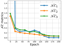
(a)

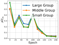
(b)

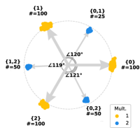
(c)

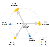
(d)

Figure 2: M-lab NC holds with imbalanced data in higher multiplicities. (a) and (b) plot metrics that measures M-lab NC on M-lab Cifar10; (c) and (d) visualize learned features on M-lab MNIST, where one multiplicity-2 class is missing in the set up which results in the reduced M-lab NC geometry. As we observe, the ETF structure for Multiplicity-1 still holds. More experimental details are deferred to Section 4.

Data imbalanced-ness in M-lab learning.

Due to the scarcity of higher multiplicity labels in the training set, in practice the imbalance of training data samples could be a more serious issue in M-lab than M-clf. It should be noted that there are two types of data imbalanced-ness: (i) the imbalanced-ness between classes within each multiplicity, and (ii) the imbalanced-ness of classes among different multiplicities. Interestingly, as long as Multiplicity-$1$ training samples remain balanced between classes, our results in Figure 2 and Figure 4 imply that the M-lab NC holds regardless of both within and among multiplicity imbalanced-ness in higher multiplicity. Given that achieving balance in Multiplicity-1 sample data is relatively easy, this implies that our result captures a common phenomenon in M-lab learning. However, if classes of Multiplicity-1 are imbalanced, we suspect a more general minority collapse phenomenon would happen [10, 55], which is worth of further investigation.

Improving M-lab prediction & training via M-lab NC.

Guided by the feature collapse phenomenon of M-lab NC, we show that we can improve the prediction accuracy and training efficiency in Section 4.2. For prediction, encoding could use an one-nearest-neighbor (ONN) approach to classify new data based on the nearest feature mean in the feature space. Empirical verification confirms that ONN encoding is more efficient and yields superior testing accuracy compared to OvA, as illustrated in Table 1. For training, as shown in Table 2, we can achieve parameter efficient training for M-lab by fixing the last layer classifier as simplex ETF and reducing the feature dimension $d$ to $K$.

Tag-wise average coefficients for M-lab ETF with high multiplicity.

The features of high multiplicity are scaled tag-wise average of Multiplicity-$1$ features, and these coefficients are simple and structured as shown in Equation 8. As illustrated in Figure 1 (i.e., $K=3$, $M=2$), the feature $\bm{h}_{i}^{\star}$ of Multiplicity-$m$ associated with class-index $S_{i}$ can be viewed as a tag-wise average of Multiplicity-$1$ features in the index set $S_{i}$. Specifically, the high multiplicity coefficients $\left\{C_{m}\right\}_{m=1}^{M}$ in Equation 8, which are shared across all features of the same multiplicity, could be expressed as

$$C_{m}=\frac{K-1}{\|\bm{W}\|_{F}^{2}}\log(\frac{K-m}{m}c_{1,m}),\quad\forall m$$

where $\left\{c_{1,m}\right\}_{m=1}^{M}$ exist.

3.2.2 Proof Ideas of Theorem 1 and Comparison with M-clf NC

We briefly outline our proofs for the global optimality in Theorem 1 as follows: essentially, our proof method first breaks down the $g(\bm{W}\bm{H}+\bm{b},\bm{Y})$ component of the objective function of Problem (4) into numerous subproblems $g_{m}(\bm{W}\bm{H}_{m}+\bm{b},\bm{Y}_{m})$, categorized by different multiplicity. We determine lower bounds for each $g_{m}$ and establish the conditions for equality attainment for each multiplicity level. Subsequently, we confirm that equality for these sets of lower bounds of different $m$ values can be attained simultaneously, thus constructing a global optimizer where the overall global objective of (4) is reached. We demonstrate that all optimizers can be recovered using this approach. As a result, our generalized proof implies M-clf NC with only single-multiplicity data.

Although our work is inspired by the recent work [75], it should be noted that our main results as well as the proving techniques used to establish them significantly differ from that of [75]. For M-lab, the derivation of optimality conditions is particularly challenging due to the combinatorial complexity of imbalanced features with higher label counts and how they interact with a single linear classifier. We elaborate on this in the following.

• We incorporate all multiplicity samples by calculating the gradient of the PAL-CE loss function to obtain the initial lower bound. The tightness condition of such bound uncovers M-lab learning’s unique “in-group and out-group” property hidden behind the combinatorial structure of high multiplicity features. Comparatively, [75] relied on Jensen’s inequality and concavity of log function which falls short under the present of high-multiplicity samples. More details can be found in Lemma 8.

• We decoupled the interplay between linear classifier across various multiplicity features by decomposing the loss into different components based on feature multiplicities. Through the decomposition, we then showed that the equality condition for each components can be achieve simultaneously. More details are provided in Lemma 2.

• We further unveil that the higher multiplicity features converge to the "scaled tag-wise average" of its associate tag feature means (Lemma 3). This requires three new supporting lemmas derived from probabilistic (Lemma 6) and matrix theory perspective (Lemma 5, 7), which is unique in M-lab learning.

3.2.3 Nonconvex Landscape Analysis

Due to the nonconvex nature of Problem (3), the characterization of global optimality alone in Theorem 1 is not sufficient for guaranteeing efficient optimization to those desired global solutions. Thus, we further study the global landscape of Problem (3) by characterizing all of its critical points, we show the following result.

Theorem 2 (Benign Optimization Landscape).

Suppose the same setting of Theorem 1, and assume the feature dimension is larger than the number of classes, i.e., $d>K$, and the number of training samples for each class are balanced within each multiplicity. Then the function $f(\bm{W},\bm{H},\bm{b})$ in Problem (4) is a strict saddle function with no spurious local minimum in the sense that:

• Any local minimizer of $f$ is a global solution of the form described in Theorem 1.

• Any critical point $(\bm{W},\bm{H},\bm{b})$ of $f$ that is not a global minimizer is a strict saddle point with negative curvatures, in the sense that there exists some direction $(\bm{\Delta}_{\bm{W}},\bm{\Delta}_{\bm{H}},\bm{\delta}_{\bm{b}})$ such that the directional Hessian $\nabla^{2}f(\bm{W},\bm{H},\bm{b})[\bm{\Delta}_{\bm{W}},\bm{\Delta}_{\bm{H}},\bm{\delta}_{\bm{b}}]<0$.

The original proof in [75] connects the nonconvex optimization problem to a convex low-rank realization and then characterizes the global optimality conditions based on the convex problem. The proof concludes by analyzing all critical points, guided by the identified optimality conditions. Because the PAL loss for M-lab is reduced from the CE loss in M-clf, the above result can be generalized from the result in [75]. We defer detailed proofs to Appendix C. Unlike Theorem 1, the result of benign landscape in Theorem 2 does not hold for $d=K-1$. The reason is that we need to construct a negative curvature direction in the null space of $\bm{W}$ for showing strict saddle points. Similar to [75], we conjecture the M-lab NC results also hold for $d=K$ and leave it for future work.

In our paper, we establish the theoretical properties of all critical points, demonstrating that the function is a strict saddle function [15] in the context of multi-label learning with respect to $(\bm{W},\bm{H})$. It’s worth noting that for strict saddle functions like PAL-CE, there exists a substantial body of prior research in the literature that provides rigorous algorithmic convergence to global minimizers. In our case, this equates to achieving a global multi-label neural collapse solution. These established methods include both first-order gradient descent techniques [15, 25, 30] and second-order trust-region methods [53], all of which ensure efficient algorithmic convergence.

4 Experiments

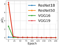
(a)

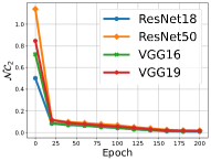
(b)

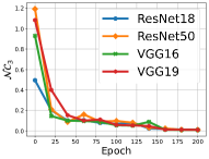
(c)

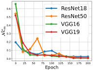
(d)

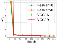
(e)

(f)

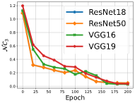
(g)

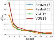
(h)

Figure 3: Prevalence of M-lab NC across different network architectures on M-lab MNIST (top) and M-lab Cifar10 (bottom). From the left to the right, the plots show the four metrics, $\mathcal{NC}_{1},\mathcal{NC}_{2},\mathcal{NC}_{3}$, and $\mathcal{NC}_{m}$, for measuring M-lab NC. More details about dataset and training setups could be found in Section A.1.

In this section, we first conduct a series of experiments to demonstrate and analyze the M-lab NC on different practical deep networks with various multi-label datasets. Second, we show that the geometric structure of M-lab NC could efficiently guide M-lablearning in both testing and training stage for better performance.

The datasets used in our experiment are real-world M-lab SVHN [42], along with synthetically generated M-lab MNIST [29] and M-lab Cifar10 [27]. The detail dataset description, generation, and visualization along with experimental setups could be found in Appendix A.

4.1 Verification of M-lab NC

Experimental demonstration of M-lab NC on practical deep networks.

When the training data (Section A.1) are balanced within multiplicities, Figure 3 shows that all practical deep networks exhibit M-lab NC during the terminal phase of training as implied by our theory. To show this, we introduce new metrics to measure M-lab NC on the last-layer features and classifiers of deep networks.

Based on theoretical results in Section 3.1, we use the original metrics $\mathcal{NC}_{1}$ (measuring the within-class variability collapse), $\mathcal{NC}_{2}$ (measuring convergence of learned classifier and feature class means to simplex ETF), and $\mathcal{NC}_{3}$ (measuring the convergence to self-duality) introduced in [44] to measure M-lab NC on Multiplicity-$1$ features $\bm{H}_{1}$ and classifier $\bm{W}$. Additionally, we also use the $\mathcal{NC}_{1}$ metric to measure variability collapse on high multiplicity features $\bm{H}_{m}\;(m>1)$. Finally, to measure M-lab ETF (the tag-wise average property) on Multiplicity-$2$ features, we propose a new angle metric $\mathcal{NC}_{m}$, which is defined as:

$$\mathcal{NC}_{m}=\frac{\text{Avg.}(\{geo_{\angle}(\overline{\bm{h}}_{i},\;\;\overline{{\bm{h}}}_{j}+\overline{{\bm{h}}}_{\ell}):(i,j,\ell)\in\mathcal{F}_{1}\})}{\text{Avg.}(\{geo_{\angle}(\overline{\bm{h}}_{i^{\prime}},\;\;\overline{{\bm{h}}}_{j^{\prime}}+\overline{{\bm{h}}}_{\ell^{\prime}}):(i^{\prime},j^{\prime},\ell^{\prime})\in\mathcal{F}_{2}\}},$$

with the sets

$$\mathcal{F}_{1} =\left\{i,j,\ell\mid|S_{i}|=2,\,|S_{j}|=|S_{\ell}|=1,\,S_{i}=S_{j}\cup S_{\ell}\right\},$$

$$\mathcal{F}_{2} =\left\{i,j,\ell\mid|S_{i}|=2,\,|S_{j}|=|S_{\ell}|=1\right\}.$$

Here, $geo{\angle}$ represents the geometric angle between two vectors, and $\overline{\bm{h}}_{i}$ is the mean of all features in the label set $S_{i}$. Intuitively, our $\mathcal{NC}_{m}$ measures the angle between features means of different label sets or classes. The numerator calculates the average angle difference between multiplicity-$2$ features means and the sum of their multiplicity-$1$ component features means. while the denominator serves as a normalization factor that is the average of all existing pairs regardless of the relationship. As training progresses, the numerator will converge to $0$, while the denominator becomes larger demonstrating the angle collapsing.

As shown in Figure 3 and Figure 4, practical networks do exhibit M-lab NC, and such a phenomenon is prevalent across network architectures and datasets. Specifically, the four metrics, evaluated on four different network architectures and two different datasets, all converge to zero as the training progresses toward the terminal phase.

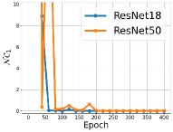
(a)

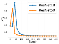
(b)

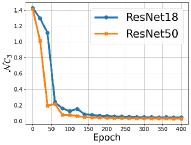
(c)

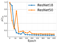
(d)

Figure 4: Prevalence of M-lab NC on the M-lab SVHN dataset. We train ResNets models on the M-lab SVHN dataset [42] for $400$ epochs and report $\mathcal{NC}_{1},\mathcal{NC}_{2},\mathcal{NC}_{3}$, and $\mathcal{NC}_{m}$, for measuring M-lab NC, respectively. See Section A.3 for more details.

M-lab NC holds despite of class imbalanced-ness in high order multiplicity labels.

Moreover, our experiments imply that maintaining balance in single-label training samples ensures the persistence of M-lab NC, even amidst imbalance in higher-order label multiplicities, across both synthetic and real-world data sets. To verify this, we create imbalanced M-lab cifar10 and MNIST datasets, and real-world M-lab SVHN dataset, with more details in Appendix A.

• Experimental results on imbalanced M-lab Cifar10 dataset. We run a ResNet18 model with this datasets (Section A.2) and report the metrics of measuring M-lab  NC in Figure 2 (a) (b). We can observe that not only $\mathcal{NC}_{1}$ to $\mathcal{NC}_{3}$ collapse to zero, but the $\mathcal{NC}_{m}$ metric is also converging zero for all $3$ groups of different size.

• Experimental results on imbalanced M-lab MNIST dataset. For Figure 2 (c) (d) on M-lab MNIST (Section A.2), we can see from the visualization of the features vectors that the scaled average property still holds despite a missing class in higher multiplicity. Here, we train a simple convolution plus multi-layer perceptron model. This implies that M-lab  NC holds even under data imbalanced-ness in high order multiplicity.

• Experimental results on imbalanced M-lab SVHN dataset. In addition, we demonstrate that M-lab NC happens independently of higher multiplicity data imbalanced-ness on real-world M-lab SVHN dataset (Section A.3). We evaluated the behavior of NC metrics on this dataset as illustrated in Figure 4, affirming the continued validity of our analysis in real-world settings.

Dataset	c10-Large		c10-Medium		c10-Small
Encoding Mechanism	OvA	ONN	OvA	ONN	OvA	ONN
Test Accuracy (%)
Overall	$78.7_{\pm 0.63}$	$\mathbf{80.5}_{\pm 0.49}$	$77.8_{\pm 0.56}$	$\mathbf{79.4}_{\pm 0.62}$	$74.0_{\pm 0.46}$	$\mathbf{76.0}_{\pm 0.32}$
Mul-1	$82.8_{\pm 0.24}$	$\mathbf{82.9}_{\pm 0.21}$	$83.2_{\pm 0.96}$	$\mathbf{83.3}_{\pm 0.97}$	$81.2_{\pm 0.18}$	$\mathbf{81.5}_{\pm 0.38}$
Mul-2	$77.5_{\pm 0.47}$	$\mathbf{79.7}_{\pm 0.65}$	$75.4_{\pm 0.57}$	$\mathbf{77.7}_{\pm 0.66}$	$69.1_{\pm 0.66}$	$\mathbf{72.3}_{\pm 0.37}$
Computational Complexity
FLOPs (B)	24.6	0.0307	19.9	0.0249	15.4	0.0192

Table 1: Test accuracy and computational complexity comparison between ONN (ours) and OvA across different multiplicity imbalance-ness. Model are trained using ResNet18 structure and average over 3 models with random initialization.

Dataset / Arch.	ResNet18		ResNet50		VGG16		VGG19
	Learned	ETF	Learned	ETF	Learned	ETF	Learned	ETF
Test IoU (%)
MLab-MNIST	99.5	99.4	99.4	99.4	99.5	99.5	99.5	99.5
MLab-Cifar10	87.7	87.7	88.9	88.6	86.9	87.4	88.7	87.0
Percentage of parameter saved (%)
MLab-MNIST	0	20.7	0	4.5	0	15.8	0	11.6
MLab-Cifar10

Table 2: Comparison of the performances and parameter efficiency between learned and fixed ETF classifier. When counting parameters, we consider all parameters that require gradient calculation during back-propagation.

4.2 Practical Implications for M-lab Learning

Finally, we show that our findings lead to improved prediction and training for M-lab learning. For prediction, Our ONN encoding approach attains greater accuracy than the OvA method with improved efficiency, eliminating the need for extra classifier training, as shown in Table 1. For training, our theory supports reducing feature dimension and maintaining a fixed classifier structure without sacrificing training accuracy as shown in Table 2. Additionally, the detail description of training dataset with experimental setup can be found in Section A.4

4.2.1 Implication I: M-lab NC guided methods for improved test performance

As discussed in Section 1, the classical OvA and PAL methods have several fundamental limitations. In this part, we show that we can improve the PAL based method by our findings. Specifically, our proposed method and comparison baseline are the following.

• Proposed one-nearest-neighbor (ONN) method: supported by the M-lab NC, features within each class collapse to their means across all multiplicities. Utilizing this, encoding new testing data into binary vectors is simplified: a one-nearest-neighbor calculation is performed between the testing data’s features and all class means.

• Classical “one-versus-all” (OvA) method: divides the task into multiple binary classification subtasks, where each needs to train an individual binary classifier for every label. During testing, thresholding is used to convert the outputs of the model (i.e., the logits) into tags.

We compared our ONN method with OvA across three synthetic M-lab Cifar-10 datasets with different data imbalanced-ness. Test accuracy is reported in table 1, where a successful prediction must perfectly match the ground truth; partial correct predictions are not counted. The detailed setup of training and dataset could be find in Section A.4. As we observe from table 1, our ONN method uniformly outperforms OvA across all data imbalanced-ness, with higher accuracy especially in higher multiplicities. Simultaneously, our ONN eliminates the necessity of training multiple binary classifiers unlike OvA, leading to substantially lower computational complexity for predictions, quantified in billions of FLOPs. Remarkably, even when dealing with the class-imbalanced real M-lab SVHN dataset, our ONN method consistently achieves an overall accuracy of $\textbf{83.6}_{\pm 0.18}\%$, surpassing $82.8_{\pm 0.42}\%$ via OvA.

4.2.2 Implication II: M-lab NC guided parameter-efficient training

With the knowledge of M-lab NC in hand, we can make direct modifications to the model architecture to achieve parameter savings without compromising performance for M-lab classification. Specifically, parameter saving could come from two folds: (i) given the existence of $\mathcal{NC}$ in the multi-label case with $d\geq K$, we can reduce the dimensionality of the penultimate features to match the number of labels (i.e., we set $d=K$); (ii) recognizing that the final linear classifier will converge to a simplex ETF as the training converges, we can initialize the weight matrix of the classifier as a simplex ETF from the start and refrain from updating it during training. By doing so, our experimental results in Table 2 demonstrate that we can achieve parameter reductions of up to $20\%$ without sacrificing the performance of the model.

5 Conclusion

In this study, we extensively analyzed the NC phenomenon in M-lab [75, 10, 23]. Based upon the UFM, our results establish that M-lab ETFs are the only global minimizers of the PAL loss function, incorporating weight decay and bias. These findings hold significant implications for improve the performance and training efficiency of M-lab tasks. We believe that our results open several interesting directions that is worth of further exploration that we discuss below.

• Dealing with data imbalanced-ness. As many multi-label datasets are imbalanced, another important direction is to investigate the more challenging cases where the Multiplicity-1 training data are imbalanced. We suspect a more general minority collapse phenomenon would happen [10, 55]. A promising approach might be employing the Simplex-Encoded-Labels Interpolation (SELI) framework, which is related to the singular value decomposition of the simplex-encoded label matrix [55]. Nonetheless, we conjecture that the scaled average property will still hold between higher multiplicity features and their multiplicity-1 features. On the other hand, when Multiplicity-1 training data are imbalanced, it is also worth studying creating a balanced dataset through data augmentation by leveraging recent advances in diffusion models [20, 57, 70].

• Designing better training loss. Prior research has underscored the significance of mitigating within-class variability collapse to improve the transferability of learned models [31]. In the context of M-labproblems, the principle of Maximal Coding Rate Reduction (MCR²) has been designed and effectively employed to foster feature diversity and discrimination, thereby preventing collapse [67, 5]. We believe that our M-lab NC could offer insights into the development of analogous loss functions for M-lablearning, with the goal of promoting diversity in features.

 

Appendix

 

Organization of Appendices

In Appendix A, We present all the datasets utilized for validating multi-label NC, guiding testing and training, along with the experimental setups introduced in this study. In Appendix B and Appendix C, we present the proofs for results from the main paper Theorem 1 (global optimality) and Theorem 2 (benign landscapes), respectively.

Appendix A Dataset Illustration and Visualization

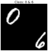
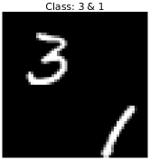
(a)

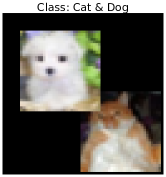
(b)

Figure 5: Illustration of synthetic multi-label MNIST (left) and Cifar10 (right) datasets.

A.1 M-lab MNIST and M-lab Cifar10 dataset

We created synthetic Multi-label MNIST [29] and Cifar10 [27] datasets by applying zero-padding to each image, increasing its width and height to twice the original size, and then combining it with another padded image from a different class. An illustration of generated multi-label samples can be found in Figure 5. To create the training dataset, for $m=1$ scenario, we randomly picked $3100$ images in each class, and for $m=2$, we generated 200 images for each combination of classes using the pad-stack method described earlier. Therefore, the total number of images in the training dataset is calculated as $10\times 3100+\binom{10}{2}\times 200=40000$. Those dataset are used to generate results in Figure 3 and Table 2.

In terms of training deep networks for M-lab, we use standard ResNet [19] and VGG [50] network architectures. Throughout all the experiments, we use an SGD optimizer with fixed batch size $128$, weight decay $(\lambda_{\bm{W}},\lambda_{\bm{H}})=(5\times 10^{-4},5\times 10^{-4})$ and momentum $0.9$. The learning rate is initially set to $1\times 10^{-1}$ and dynamically decays to $1\times 10^{-3}$ following a CosineAnnealing learning rate scheduler as described in [35]. The total number of epochs is set to $200$ for all experiments.

A.2 Multiplicity 2 imbalanced M-lab MNIST and M-lab Cifar10 dataset

Following the same padding rule described in Section A.1, the multiplicity-2 imbalanced data used to generate Figure 2 are created as follows. The cifar10 dataset has balanced Multiplicity-$1$ samples ($5000$ for each class). For the classes of Multiplicity-$2$, we divide them into $3$ groups: the large group ($500$ samples), the middle group ($50$ samples), and the small group ($5$ samples).

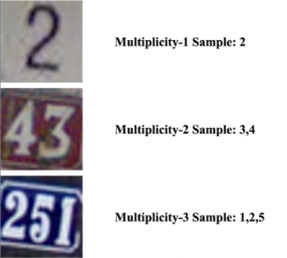
(a)

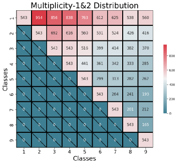
(b)

Figure 6: Illustration of M-lab SVHN dataset. As illustrated in (a), the Street View House Numbers (SVHN) Dataset [42] comprises labeled numerical characters and inherently serves as a M-lab learning dataset. We applied minimal preprocessing to achieve balance specifically within the Multiplicity-1 scenario, as evidenced by the diagonal entries in (b). Furthermore, we omitted samples with Multiplicity-4 and above, as these images posed considerable recognition challenges. Notably, the Multiplicity-2 case remained largely imbalanced, as observed in the off-diagonal entries in (b). Nonetheless, our findings remained robust and consistent in this scenario, as evidenced in Figure 4.

A.3 Multiplicity 2 imbalanced M-lab SVHN dataset

To further explore our findings, we conducted additional experiments on the practical SVHN dataset [42] alongside the synthetic datasets. In order to preserve the natural characteristics of the SVHN dataset, we applied minimal pre-processing only to ensure a balanced scenario for multiplicity-1, while leaving other aspects of the dataset untouched. The dataset are visualized in Figure 6.

A.4 Dataset used to compare test accuracy and efficiency between ONN and OvA

For training dataset, following the same generation method described in Section A.1 and symply varying data balanced-ness, the synthetic multiplicity imbalanced data used in Table 1 are generated from Cifar10 datasets. All $3$ datasets has $1500$ sample in every class in multiplicity-1, we reduce the sample in every class in multiplicity-2 to $1000$, $750$, and $500$, resulting in the “c10-Large", “c10-Medium", and “c10-Small" datasets. The testing datasets are independently generated, each with a sample size equivalent to $20\%$ of the training datasets.

Standard ResNet [19] network architecture are used for training with only fixing the last layer classifier of as $ETF$. The SGD optimizer with fixed batch size $128$ are used. Specifically, for the three Cifar-10 datasets, models are trained with weight decay $(\lambda_{\bm{W}},\lambda_{\bm{H}})=(5\times 10^{-5},10^{-5})$ with $200$ epochs with learning rate of $0.1$. For the SVHN dataset, models are trained with weight decay $(\lambda_{\bm{W}},\lambda_{\bm{H}})=(5\times 10^{-6},1.5\times 10^{-6})$ with $100$ epochs with learning rate of $0.09$. For testing with OvA, the additional linear classifiers are trained until the training loss reaches $0$, typically after approximately $2$ epochs.

Appendix B Optimality Condition

The purpose of this section is to prove Theorem 1. As such, throughout this section, we assume that we are in the situation of the statement of said theorem. Due to the additional complexity of the M-lab setting compared to the M-clf setting, analysis of the M-lab NC requires substantially more notations. These notations, which are defined in section B.1, while not necessary for stating Theorem 1, are crucial for the proofs in section B.2 .

B.1 Additional notations

For the reader’s convenience, we recall the following:

$$N :=\mbox{number of samples}$$ (9)

$$N_{m} :=\mbox{number of samples $i\in[N]$ such that $|S_{i}|=m$}$$ (10)

$$n_{m} :=N_{m}/\binom{K}{m}$$ (11)

$$\binom{[K]}{m} :=\{S\subseteq[K]:|S|=m\}$$ (12)

$$M :=\mbox{largest $m$ such that $n_{m}\neq 0$}$$ (13)

$$d :=\mbox{dimension of the last layer features}$$ (14)

B.1.1 Lexicographical ordering on subsets

For each $m\leq K$, recall from the above that the set of subsets of $[K]$ of size $m$ is denoted by the commonly used, suggestive notation $\binom{[K]}{m}$. Moreover, $|\binom{[K]}{m}|=\binom{K}{m}$.

$\rhd$ Notation convention. Assume the lexicographical ordering on $\binom{[K]}{m}$. Thus, for each $k\in\binom{K}{m}$, the $k$-th subset of $\binom{[K]}{m}$ is well-defined.

For example, when $K=5$ and $m=2$, there are $\binom{5}{2}=10$ elements in $\binom{[5]}{2}$ which, when listed in the lexicographic ordering, are

$$\underbrace{\{1,2\}}_{\mbox{1st}},\underbrace{\{1,3\}}_{\mbox{2nd}},\underbrace{\{1,4\}}_{\mbox{3rd}},\underbrace{\{1,5\}}_{\mbox{4th}},\underbrace{\{2,3\}}_{\cdots},\{2,4\},\{2,5\},\{3,4\},\{3,5\},\underbrace{\{4,5\}}_{\mbox{10th}}.$$

In general, we use the notation $S_{m,k}$ to denote the $k$-th subset of $\binom{[K]}{m}$. In other words,

$$\binom{[K]}{m}=\{S_{m,1},\,\,S_{m,2},\,\,\dots,\,\,S_{m,\binom{K}{m}}\}.$$

B.1.2 Block submatrices of the last layer feature matrix

Without the loss of generality, we assume that the sample indices $i\in[N]$ are sorted such that $|S_{i}|$ is non-decreasing, i.e., $|S_{1}|\leq\cdots\leq|S_{i}|\leq\cdots\leq|S_{N}|.$ Clearly, this does not affect the optimization problem itself. Denote the set of indices of Multiplicity-$m$ samples by $\mathcal{I}_{m}:=\{i\in[N]:|S_{i}|=m\}$. Thus, we have

$$\mathcal{I}_{1}=\{1,\dots,N_{1}\},\,\,\mathcal{I}_{2}=\{1+N_{1},\dots,N_{2}+N_{1}\},\,\,\cdots\mathcal{I}_{m}=\{1+\sum_{\ell=1}^{m}N_{\ell},\dots,N_{m}+\sum_{\ell=1}^{m}N_{\ell}\},\cdots\,\,$$

Below, it will be helpful to define the notation

$$\mathcal{I}_{m,S}:=\{i\in[N]:S_{i}=S\}$$

for each $m=1,\dots,M$ and $S\in\binom{[K]}{m}$.

$\rhd$ Notation convention. Define the block-submatrices $\bm{H}_{1},\dots,\bm{H}_{M}$ of $\bm{H}$ such that

1. $\bm{H}_{m}\in\mathbb{R}^{d\times N_{m}}$

2. $\bm{H}=\begin{bmatrix}\bm{H}_{1}&\bm{H}_{2}&\cdots&\bm{H}_{M}\end{bmatrix}$

Thus, as in the main paper, the columns of $\bm{H}_{m}$ correspond to the features of $\mathcal{I}_{m}$.

B.1.3 Decomposition of the PAL-CE loss

Define

$$g_{m}(\bm{W}\bm{H}_{m}+\bm{b},\bm{Y}):=\frac{1}{N_{m}}\sum_{i\in\mathcal{I}_{m}}\underline{\mathcal{L}}_{\mathtt{PAL}}(\bm{W}\bm{h}_{i}+\bm{b},\bm{y}_{S_{i}}).$$ (15)

Intuitively, $g_{m}$ is the contribution to $g$ from the Multiplicity-$m$ samples. More precisely, the function $g(\bm{W}\bm{H}+\bm{b},\bm{Y})$ from Equation 4 can be decomposed as

$$g(\bm{W}\bm{H}+\bm{b},\bm{Y})=\sum_{m=1}^{M}\frac{N_{m}}{N}g_{m}(\bm{W}\bm{H}_{m}+\bm{b},\bm{Y}).$$ (16)

B.1.4 Triple indices notation

Next, we state precisely the data balanced-ness condition from Theorem 1. In order to state the condition, we need some additional notations. Fix some $m\in\{1,\dots,M\}$ and let $S\in\binom{[K]}{m}$. Define

$$n_{m,S}:=\{i\in[N]:S_{i}=S\}.$$ (17)

Theorem 1 made the following data balanced-ness condition:

$$n_{m,S}=N_{m}/\binom{K}{m}=:n_{m} S\in\binom{[K]}{m}$$ for all . (18)

In other words, for a fixed $m\in[M]$, the set $\mathcal{I}_{m,S}$ has the same constant cardinality equal to $n_{m}$ ranging across all $S\in\binom{[K]}{m}$.

By the data balanced-ness condition, we have for a fixed $m=1,\dots,M$ that $\mathcal{I}_{m,S}$ have the same number of elements across all $S\in\binom{[K]}{m}$. Moreover, in our notation, we have $|\mathcal{I}_{m,S}|=n_{m}$. Below, for each $m=1,\dots,M$ and for each $S\in\binom{[K]}{m}$, choose an arbitrary ordering on $\mathcal{I}_{m,S}$ once and for all. Every sample is uniquely specified by the following three indices:

1. $m\in[M]$ the sample’s multiplicity, i.e., $m=|S|$

2. $k\in\binom{K}{m}$ the index such that $S_{m,k}$ is the label set of the sample,

3. $i\in[n_{m}]$ such that the sample is the $i$-th element of $\mathcal{I}_{m,S_{m,k}}$.

More concisely, we now introduce the

$\rhd$ Notation convention. Denote each sample by the triplet

$$(m,k,i)\quad\mbox{where}\quad m\in[M],\,\,k\in\binom{K}{m},\,\,i\in[n_{m}].$$ (19)

Below, (19) will be referred to as the triple indices notation and every sample will be referred to by its triple indices $(m,k,i)$ instead of the previous single index $i\in[N]$. Accordingly, throughout the appendix, columns of $\bm{H}$ are expressed as $\bm{h}_{m,k,i}$ instead of the previous $\bm{h}_{i}$, and thus the block submatrix $\bm{H}_{m}$ of $\bm{H}$ can be, without the loss of generality, be written as $\bm{H}_{m}=\begin{bmatrix}\bm{h}_{m,k,i}\end{bmatrix}_{m\in[M],\,\,k\in\binom{K}{m},\,\,i\in[n_{m}]}.$

Moreover, in the triple indices notation, Equation 15 can be rewritten as

$$g_{m}(\bm{W}\bm{H}_{m}+\bm{b})=\frac{1}{N_{m}}\sum_{i=1}^{n_{m}}\sum_{k=1}^{\binom{K}{m}}{\mathcal{L}_{\mathtt{PAL}}(\bm{W}\bm{h}_{m,k,i},\bm{y}_{S_{m,k}})}$$ (20)

B.2 Proofs

We will first state the proof of Theorem 1 which depends on several lemmas appearing later in the section. Thus, the proof of Theorem 1 serves as a roadmap for the rest of this section.

Proof of Theorem 1.

Recall the definition of a coercive function: a function $\varphi:\mathbb{R}^{n}\to\mathbb{R}$ is said to be coercive if $\lim_{\|x\|\to\infty}\varphi(x)=+\infty$. It is well-known that a coercive function attains its infimum which is a global minimum.

Now, note that the objective function $f(\bm{W},\bm{H},\bm{b})$ in Problem (4) is coercive due to the weight decay regularizers (the terms $\|\bm{W}\|_{F}^{2}$, $\|\bm{H}\|_{F}^{2}$ and $\|\bm{b}\|_{F}^{2}$) and that the pick-all-labels cross-entropy loss is non-negative. Thus, a global minimizer, denoted below as $(\bm{W},\bm{H},\bm{b})$, of Problem (4) exists. By Lemma B.2, we know that any critical point $(\bm{W},\bm{H},\bm{b})$ of Problem (4) satisfies

$$\bm{W}^{\top}\bm{W}=\frac{\lambda_{\bm{H}}}{\lambda_{\bm{W}}}\bm{H}\bm{H}^{\top}.$$

Let $\rho:=\|\bm{W}\|_{F}^{2}$. Thus, $\|\bm{H}\|_{F}^{2}=\frac{\lambda_{\bm{W}}}{\lambda_{\bm{H}}}\rho$

We first provide a lower bound for the PAL cross-entropy term $g(\bm{W}\bm{H}+\bm{b}\bm{1}^{\top})$ and then show that the lower bound is tight if and only if the parameters are in the form described in Theorem 1. For each $m=1,\dots,M$, let $c_{1,m}>0$ be arbitrary, to be determined below. Now by Lemma 2 and Lemma 8, we have

$$g(\bm{W}\bm{H}+\bm{b})-\Gamma_{2}\geq-\frac{1}{N}\sqrt{\sum_{m=1}^{M}\left(\frac{1}{1+c_{1,m}}\frac{m}{K-m}\right)^{2}\kappa_{m}n_{m}\binom{K}{m}^{2}}\sqrt{\frac{\lambda_{\bm{W}}}{\lambda_{\bm{H}}}}\rho$$

where $\Gamma_{2}:=\sum_{m=1}^{M}c_{2,m}$ and $c_{2,m}$ is as in Lemma 8. Therefore, we have

$$f(\bm{W},\bm{H},\bm{b}) =g(\bm{W}\bm{H}+\bm{b}^{\top})+\lambda_{\bm{W}}\|\bm{W}\|_{F}^{2}+\lambda_{\bm{H}}\|\bm{H}\|_{F}^{2}+{\lambda_{\bm{b}}}\|\bm{b}\|_{2}^{2}$$

$$\geq-\frac{1}{N}\sqrt{\sum_{m=1}^{M}\left(\frac{1}{1+c_{1,m}}\frac{m}{K-m}\right)^{2}\kappa_{m}n_{m}\binom{K}{m}^{2}}\sqrt{\frac{\lambda_{\bm{W}}}{\lambda_{\bm{H}}}}\rho+\Gamma_{2}+2\lambda_{\bm{W}}\rho+\frac{\lambda_{\bm{b}}}{2}\|\bm{b}\|_{2}^{2}$$

$$\geq-\frac{1}{N}\sqrt{\sum_{m=1}^{M}\left(\frac{1}{1+c_{1,m}}\frac{m}{K-m}\right)^{2}\kappa_{m}n_{m}\binom{K}{m}^{2}}\sqrt{\frac{\lambda_{\bm{W}}}{\lambda_{\bm{H}}}}\rho+\Gamma_{2}+2\lambda_{\bm{W}}\rho$$ (21)

where the last inequality becomes an equality whenever either $\lambda_{\bm{b}}=0$ or $\bm{b}=\bm{0}$. Furthermore, by Lemma 3, we know that the Inequality (21) becomes an equality if and only if $(\bm{W},\bm{H},\bm{b})$ satisfy the following:

$$\mbox{(I)}\quad\|\bm{w}^{1}\|_{2}=\|\bm{w}^{2}\|_{2}=\cdots=\|\bm{w}^{K}\|_{2},\quad\mbox{and}\quad\bm{b}=b\bm{1},$$

$$\mbox{(II)}\quad\frac{1}{\binom{K}{m}}\sum_{k=1}^{\binom{K}{m}}\bm{h}_{m,k,i}=\bm{0},\quad\mbox{and}\quad\sqrt{\frac{\binom{K-2}{m-1}}{n_{m}}}\bm{w}^{k}=\sum_{\ell:k\in S_{m,\ell}}{\bm{h}_{m,\ell,i}},\forall m\in[M],k\in[K],i\in[n_{m}],$$

$$\mbox{(III)}\qquad\bm{W}^{\top}\bm{W}=\frac{\rho}{K-1}\left(\bm{I}_{K}-\frac{1}{K}\bm{1}_{K}\bm{1}_{K}^{\top}\right)$$

(IV) There exist unique positive real numbers $C_{1},C_{2},\dots,C_{M}>0$ such that the following holds:

$$\bm{h}_{1,k,i}=C_{1}\bm{w}^{\ell}\quad\qquad\qquad\mbox{when}\,\,S_{1,k}=\{\ell\},\;\ell\in[K], =1$$ (Multiplicity Case)

$$\bm{h}_{m,k,i}=C_{m}\textstyle{\sum_{\ell\in S_{m,k}}}\bm{w}^{\ell}\quad\mbox{when}\,\,m>1. >1$$ (Multiplicity Case)

Note that condition (IV) is a restatement of Equation 7 and Equation 8. The choice of the $c_{1,m}$’s is given by (V) from Lemma 3. ∎

Lemma 1.

we have:

$$\bm{W}^{\top}\bm{W}=\frac{\lambda_{\bm{H}}}{\lambda_{\bm{W}}}\bm{H}\bm{H}^{\top}\quad and\quad\rho=\|\bm{W}\|_{F}^{2}=\frac{\lambda_{\bm{H}}}{\lambda_{\bm{W}}}\|\bm{H}\|_{F}^{2}$$

Proof.

The proceeds identically as in given by [75] Lemma B.2 and is thus omitted here. ∎

The following lemma is the generalization of [75] Lemma B.3 to the multilabel case for each multiplicity.

Lemma 2.

Let $(\bm{W},\bm{H},\bm{b})$ be a critical point for the objective $f$ from Problem (4). Let $c_{1,m}>0$ be arbitrary and let $\gamma_{1,m}:=\frac{1}{1+c_{1,m}}\frac{m}{K-m}$. Define $\kappa_{m}:=\left(\frac{K}{m\binom{K}{m}}\right)^{2}\binom{K-2}{m-1}$. Then

$$g(\bm{W}\bm{H}+\bm{b})-\Gamma_{2}\geq-\frac{1}{N}\sqrt{\sum_{m=1}^{M}\left(\frac{1}{1+c_{1,m}}\frac{m}{K-m}\right)^{2}\kappa_{m}n_{m}\binom{K}{m}^{2}}\sqrt{\frac{\lambda_{\bm{W}}}{\lambda_{\bm{H}}}}\rho.$$ (22)

where $\rho:=\|\bm{W}\|_{F}^{2}$, $\Gamma_{2}:=\sum_{m=1}^{M}c_{2,m}$ and $c_{2,m}$ is as in Lemma 8.

Note that $\Gamma_{2}$ depends on $c_{1,1},\,c_{1,2},\,\dots,\,c_{1,M}$ because $c_{2,m}$ depends on $c_{1,m}$ for each $m\in[M]$.

Proof.

Throughout this proof, let $\bm{z}_{m,k,i}:=\bm{W}\bm{h}_{m,k,i}+\bm{b}$ and choose the same $\gamma_{1,m},c_{2,m}$ for all $i$ and $k$. The first part of this proof aim to find the lower bound for each $g_{m}(\bm{W},\bm{H}_{m},\bm{b})$ along with conditions when the bound is tight. The rest of the proof focus on sum up $g_{m}$ to get Equation 22. Thus, using Equation 20 with the $\bm{z}_{m,k,i}$’s, we have that $g_{m}$ can be written as

$$g_{m}(\bm{W}\bm{H}_{m}+\bm{b}) =\frac{1}{N_{m}}\sum_{i=1}^{n_{m}}\sum_{k=1}^{\binom{K}{m}}{\underline{\mathcal{L}}_{\mathtt{PAL}}(\bm{z}_{m,k,i},\bm{y}_{S_{m,k}})}$$ (23)

By directly applying Lemma 8, the following lower bound holds:

$$N_{m}g_{m}(\bm{W}\bm{H}_{m}+\bm{b}) \geq\gamma_{1,m}\sum_{i=1}^{n_{m}}\sum_{k=1}^{\binom{K}{m}}{\langle\bm{1}-\tfrac{K}{m}\mathbb{I}_{S},\,\bm{W}\bm{h}_{m,k,i}+\bm{b}\rangle}+N_{m}c_{2,m}$$

which implies that

$$\ \quad\gamma_{1,m}^{-1}(g_{m}(\bm{W}\bm{H}_{m}+\bm{b})-c_{2,m})$$

$$\geq\frac{1}{N_{m}}\sum_{i=1}^{n_{m}}\sum_{k=1}^{\binom{K}{m}}{\langle\bm{1}-\tfrac{K}{m}\mathbb{I}_{S},\,\bm{W}\bm{h}_{m,k,i}+\bm{b}\rangle}$$

$$=\frac{1}{N_{m}}\sum_{i=1}^{n_{m}}\underbrace{\sum_{k=1}^{\binom{K}{m}}{\langle\bm{1}-\tfrac{K}{m}\mathbb{I}_{S},\,\bm{W}\bm{h}_{m,k,i}\rangle}}_{(\star)}+\frac{1}{N_{m}}\sum_{i=1}^{n_{m}}\underbrace{\sum_{k=1}^{\binom{K}{m}}{\langle\bm{1}-\tfrac{K}{m}\mathbb{I}_{S},\bm{b}\rangle}}_{(\star\star)}$$ (24)

To further simplify the inequality above, we break it down into two parts, namely, the feature part ($\star$) and the bias part ($\star\star$) and analyze each of them separately. We first show that the term ($\star\star$) is equal to zero. To see this, note that

$$(\star\star) =\sum_{k=1}^{\binom{K}{m}}\left(\sum_{j=1}^{K}{b_{j}}-\frac{K}{m}\sum_{j^{\prime}\in S_{m,k}}{b_{j^{\prime}}}\right)$$

$$=\sum_{k=1}^{\binom{K}{m}}\sum_{j=1}^{K}{b_{j}}-\frac{K}{m}\sum_{k=1}^{\binom{K}{m}}\sum_{j^{\prime}\in S_{m,k}}{b_{j^{\prime}}}$$

$$=K\binom{K}{m}\bar{b}-\frac{K}{m}m\binom{K}{m}\bar{b}$$

$$=0$$ (25)

where $\bar{b}=\frac{1}{K}\sum_{j=1}^{K}{b_{j}}$ and $\sum_{k=1}^{\binom{K}{m}}\sum_{j=1}^{K}{b_{j}}=K\binom{K}{m}\bar{b}$. Thus

$$\sum_{k=1}^{\binom{K}{m}}\sum_{j^{\prime}\in S_{m,k}}b_{j^{\prime}}\overset{(\diamondsuit)}{=}\sum_{j=1}^{K}\sum_{k:j\in S_{m,k}}b_{j}{=}\sum_{j=1}^{K}b_{j}\#\{k:j\in S_{m,k}\}=\sum_{j=1}^{K}\binom{K}{m}\frac{m}{K}b_{j}=m\binom{K}{m}\overline{b}.$$

Note that the equality at $(\diamondsuit)$ holds by switching the order of the summation. Now, substituting the result of Equation 25 into the Inequality (24), we have the new lower bound of $g_{m}$:

$$\gamma_{1,m}^{-1}(g_{m}(\bm{W}\bm{H}_{m}+\bm{b})-c_{2,m}) \geq\frac{1}{N_{m}}\sum_{i=1}^{n_{m}}\underbrace{\sum_{k=1}^{\binom{K}{m}}{\langle\bm{1}-\tfrac{K}{m}\mathbb{I}_{S},\,\bm{W}\bm{h}_{m,k,i}\rangle}}_{(\star)}$$ (26)

and the bound is tight when conditions are met in Lemma 8. To simplify the expression $(\star)$ we first distribute the outer layer summation and further simplify it as:

$$(\star) =\sum_{k=1}^{\binom{K}{m}}\sum_{j=1}^{K}{\bm{h}_{m,k,i}^{\top}\cdot\bm{w}^{j}}-\frac{K}{m}\sum_{k=1}^{\binom{K}{m}}\sum_{j^{\prime}\in S_{m,k}}{\bm{h}_{m,k,i}^{\top}\cdot\bm{w}^{j^{\prime}}}$$

$$=\sum_{k=1}^{\binom{K}{m}}\sum_{j=1}^{K}{\bm{h}_{m,k,i}^{\top}\cdot\bm{w}^{j}}-\frac{K}{m}\sum_{j=1}^{K}\sum_{k^{\prime}:j\in S_{k^{\prime}}}\bm{h}_{m,k^{\prime},i}^{\top}\bm{w}^{j}$$ (27)

$$=\sum_{k=1}^{\binom{K}{m}}\sum_{j=1}^{K}{\bm{h}_{m,k,i}^{\top}\cdot\bm{w}^{j}}-\frac{K}{m}\sum_{j=1}^{K}\bm{h}_{m,\{j\},i}^{\top}\bm{w}^{j}$$

$$=\sum_{j=1}^{K}\sum_{k=1}^{\binom{K}{m}}{\bm{h}_{m,k,i}^{\top}\cdot\bm{w}^{j}}-\frac{K}{m}\sum_{j=1}^{K}\bm{h}_{m,\{j\},i}^{\top}\bm{w}^{j}$$ (28)

$$=\sum_{j=1}^{K}\left(\sum_{k=1}^{\binom{K}{m}}{\bm{h}_{m,k,i}}-\frac{K}{m}\bm{h}_{m,\{j\},i}\right)^{\top}\bm{w}^{j}$$

$$=\sum_{j=1}^{K}\left(\binom{K}{m}\overline{\bm{h}}_{m,\bullet,i}-\frac{K}{m}\bm{h}_{m,\{j\},i}\right)^{\top}\bm{w}^{j}$$ (29)

where we let $\bm{h}_{m,\{j\},i}=\sum_{k:j\in S_{m,k}}{\bm{h}_{m,k,i}}$ and $\overline{\bm{h}}_{m,\bullet,i}$ be the “average” of $\bm{h}_{m,k,i}$ over all $k\in\binom{K}{m}$ defined as:

$$\overline{\bm{h}}_{m,\bullet,i}:=\frac{1}{\binom{K}{m}}\sum_{k=1}^{\binom{K}{m}}\bm{h}_{m,k,i}.$$ (30)

Similarly to $(\diamondsuit)$, the Equations (27) and (28) holds since we only switch the order of summation. Continuing simplification, we substitute the result in Equations (29) and (25) into Inequality (24) we have:

$$\gamma_{1,m}^{-1}(g_{m}(\bm{W}\bm{H}_{m}+\bm{b})-c_{2,m}) \geq\frac{1}{N_{m}}\sum_{i=1}^{n_{m}}{\sum_{j=1}^{K}\left(\binom{K}{m}\overline{\bm{h}}_{m,\bullet,i}-\frac{K}{m}\bm{h}_{m,\{j\},i}\right)^{\top}\bm{w}^{j}}$$

$$=\frac{1}{N_{m}}\sum_{i=1}^{n_{m}}{\sum_{k=1}^{K}\left(\binom{K}{m}\overline{\bm{h}}_{m,\bullet,i}-\frac{K}{m}\bm{h}_{m,\{k\},i}\right)^{\top}\bm{w}^{k}}$$

$$=\frac{1}{n_{m}}\sum_{i=1}^{n_{m}}{\sum_{k=1}^{K}\left(\overline{\bm{h}}_{m,\bullet,i}-\frac{K}{m\binom{K}{m}}\bm{h}_{m,\{k\},i}\right)^{\top}\bm{w}^{k}}$$

Further more, from the AM-GM inequality (e.g., see Lemma A.2 of [75]), we know that for any $\bm{u}$, $\bm{v}\in\mathbb{R}^{K}$ and any $c_{3,m}>0$,

$$\bm{u}^{\top}\bm{v}\leq\frac{c_{3,m}}{2}\|\bm{u}\|_{2}^{2}+\frac{1}{2c_{3,m}}\|\bm{v}\|_{2}^{2}$$ (31)

where the above AM-GM inequality becomes an equality when $c_{3,m}\bm{u}=\bm{v}$. Thus letting $\bm{u}=\bm{w}^{k}$ and $\bm{v}=\left(\overline{\bm{h}}_{m,\bullet,i}-\frac{K}{m\binom{K}{m}}\bm{h}_{m,\{k\},i}\right)^{\top}$ and applying the AM-GM inequality, we further have:

$$\gamma_{1,m}^{-1}(g_{m}(\bm{W}\bm{H}_{m}+\bm{b})-c_{2,m})$$

$$\geq\frac{1}{n_{m}}\sum_{i=1}^{n_{m}}{\sum_{k=1}^{K}\left(\overline{\bm{h}}_{m,\bullet,i}-\frac{K}{m\binom{K}{m}}\bm{h}_{m,\{k\},i}\right)^{\top}\bm{w}^{k}}$$ (32)

$$\geq\frac{1}{n_{m}}\sum_{i=1}^{n_{m}}\sum_{k=1}^{K}{\left(-\frac{c_{3,m}}{2}\|\bm{w}^{k}\|_{2}^{2}-\frac{1}{2c_{3,m}}\|\overline{\bm{h}}_{m,\bullet,i}-\frac{K}{m\binom{K}{m}}\bm{h}_{m,\{k\},i}\|_{2}^{2}\right)}$$

$$=\frac{1}{n_{m}}\sum_{i=1}^{n_{m}}\sum_{k=1}^{K}{-\frac{c_{3,m}}{2}\|\bm{w}^{k}\|_{2}^{2}}-\frac{1}{n_{m}}\sum_{i=1}^{n_{m}}\sum_{k=1}^{K}{\frac{1}{2c_{3,m}}\|\overline{\bm{h}}_{m,\bullet,i}-\frac{K}{m\binom{K}{m}}\bm{h}_{m,\{k\},i}\|_{2}^{2}}$$

$$=-\frac{c_{3,m}}{2}\|\bm{W}\|_{F}^{2}-\frac{1}{2c_{3,m}n_{m}}\sum_{i=1}^{n_{m}}\sum_{k=1}^{K}{\|\overline{\bm{h}}_{m,\bullet,i}-\frac{K}{m\binom{K}{m}}\bm{h}_{m,\{k\},i}\|_{2}^{2}}$$

$$=-\frac{c_{3,m}}{2}\|\bm{W}\|_{F}^{2}-\frac{1}{2c_{3,m}n_{m}}\sum_{i=1}^{n_{m}}\Big{(}K{\|\overline{\bm{h}}_{m,\bullet,i}\|_{2}^{2}}+\left(\frac{K}{m\binom{K}{m}}\right)^{2}\left(\sum_{k=1}^{K}{\|\bm{h}_{m,\{k\},i}\|_{2}^{2}}\right)$$

$$\qquad\qquad\qquad\qquad\qquad\qquad\qquad\qquad\qquad\qquad\qquad\qquad-2K\langle\overline{\bm{h}}_{m,\bullet,i},\ \overline{\bm{h}}_{m,\bullet,i}\rangle\Big{)}$$

$$=-\frac{c_{3,m}}{2}\|\bm{W}\|_{F}^{2}-\frac{1}{2c_{3,m}n_{m}}\sum_{i=1}^{n_{m}}\left(\left(\frac{K}{m\binom{K}{m}}\right)^{2}\left(\sum_{k=1}^{K}{\|\bm{h}_{m,\{k\},i}\|_{2}^{2}}\right)-K\|\overline{\bm{h}}_{m,\bullet,i}\|_{2}^{2}\right)$$

$$=-\frac{c_{3,m}}{2}\|\bm{W}\|_{F}^{2}-\frac{\left(\frac{K}{m\binom{K}{m}}\right)^{2}}{2c_{3,m}n_{m}}\sum_{i=1}^{n_{m}}\left(\sum_{k=1}^{K}{\|\bm{h}_{m,\{k\},i}\|_{2}^{2}}-K\|\overline{\bm{h}}_{m,\bullet,i}\|_{2}^{2}\right)$$

$$\geq-\frac{c_{3,m}}{2}\|\bm{W}\|_{F}^{2}-\frac{\left(\frac{K}{m\binom{K}{m}}\right)^{2}}{2c_{3,m}n_{m}}\sum_{i=1}^{n_{m}}\sum_{k=1}^{K}{\|\bm{h}_{m,\{k\},i}\|_{2}^{2}}$$ (33)

$$=-\frac{c_{3,m}}{2}\|\bm{W}\|_{F}^{2}-\frac{\left(\frac{K}{m\binom{K}{m}}\right)^{2}}{2c_{3,m}n_{m}}\left(\|\bm{H}_{m}\bm{D}_{m}\|_{F}^{2}\right)$$ (34)

$$=-\frac{c_{3,m}}{2}\|\bm{W}\|_{F}^{2}-\frac{\left(\frac{K}{m\binom{K}{m}}\right)^{2}\binom{K-2}{m-1}}{2c_{3,m}n_{m}}\left(\|\bm{H}_{m}\|_{F}^{2}\right)\quad\quad\quad\quad\quad\quad(\mbox{by \lx@cref{creftypecap~refnum}{lemma:pascal_norm}})$$

$$=-\frac{c_{3,m}}{2}\|\bm{W}\|_{F}^{2}-\frac{\kappa_{m}}{2c_{3,m}n_{m}}\left(\|\bm{H}_{m}\|_{F}^{2}\right),$$

where we let $\bm{D}_{m}=\mbox{diag}(\bm{Y}_{m}^{\top},\cdots,\bm{Y}_{m}^{\top})\in\mathbb{R}^{(n_{m}*\binom{K}{m})\times(n_{m}*K)}$ and $\bm{Y}_{m}\in\mathbb{R}^{K\times\binom{K}{m}}$ is the many-hot label matrix defined as follows:

$$\bm{Y}_{m}=\begin{bmatrix}\bm{y}_{S_{m,k}}\end{bmatrix}_{k\in\binom{K}{m}}.$$

The first Inequality (32) is tight whenever conditions mentioned in Lemma 8 are satisfied and the second inequality is tight if and only if

$$c_{3,m}\bm{w}^{k}=\left(\frac{K}{m\binom{K}{m}}\bm{h}_{m,\{k\},i}-\overline{\bm{h}}_{m,\bullet,i}\right)\quad\forall k\in[K],\quad i\in[n_{m}].$$ (35)

Therefore, we have

$$g_{m}(\bm{W}\bm{H}_{m}+\bm{b})-c_{2,m}\geq-\gamma_{1,m}\frac{c_{3,m}}{2}\|\bm{W}\|_{F}^{2}-\gamma_{1,m}\frac{\kappa_{m}}{2c_{3,m}n_{m}}\left(\|\bm{H}_{m}\|_{F}^{2}\right).$$ (36)

The last Inequality (33) achieves its equality if and only if

$$\overline{\bm{h}}_{m,\bullet,i}=\bm{0},\quad\forall i\in[n_{m}].$$ (37)

Plugging this into (Equation 35), we have

$$c_{3,m}\bm{w}^{k} =\frac{K}{m\binom{K}{m}}\bm{h}_{m,\{k\},i}$$

$$\implies c_{3,m}^{2} =\frac{\left(\frac{K}{m\binom{K}{m}}\right)^{2}\sum_{i=1}^{n}\sum_{k=1}^{K}{\|\bm{h}_{m,\{k\},i}\|_{F}^{2}}}{n_{m}\sum_{k=1}^{K}{\|\bm{w}^{k}}\|_{2}^{2}}$$

$$=\frac{\left(\frac{K}{m\binom{K}{m}}\right)^{2}\binom{K-2}{m-1}\|\bm{H}_{m}\|_{F}^{2}}{n_{m}\|\bm{W}\|_{F}^{2}}$$

$$=\frac{\kappa_{m}}{n_{m}}\frac{\|\bm{H}_{m}\|_{F}^{2}}{\|\bm{W}\|_{F}^{2}}$$

$$\implies c_{3,m} =\sqrt{\frac{\kappa_{m}}{n_{m}}}\frac{\|\bm{H}_{m}\|_{F}}{\|\bm{W}\|_{F}}$$

$$\implies c_{3,m}^{2} =\frac{\kappa_{m}}{n_{m}}\frac{\|\bm{H}_{m}\|_{F}^{2}}{\|\bm{W}\|_{F}^{2}}.$$

Now, note that by our definition of $\rho$ and Lemma 1, we get

$$\|\bm{H}\|_{F}^{2}=\frac{\lambda_{\bm{W}}}{\lambda_{\bm{H}}}\rho.$$ (38)

Recall from the state of the lemma that we defined $\kappa_{m}:=\left(\frac{K/m}{\binom{K}{m}}\right)^{2}\binom{K-2}{m-1}$ and that $\gamma_{1,m}:=\frac{1}{1+c_{1,m}}\frac{m}{K-m}$. Thus, continuing from Inequality (36), we have

$$\gamma_{1,m}^{-1}(g_{m}(\bm{W}\bm{H}_{m}+\bm{b})-c_{2,m})\geq-\frac{c_{3,m}}{2}\|\bm{W}\|_{F}^{2}-\frac{\kappa_{m}}{2c_{3,m}n_{m}}\|\bm{H}_{m}\|_{F}^{2}.$$

Next, let $Q>0$ be an arbitrary constant, to be determined later such that

$$\gamma_{1,m}=\frac{1}{N_{m}}Qc_{3,m}^{-1}\frac{\|\bm{H}_{m}\|_{F}^{2}}{\|\bm{W}\|_{F}^{2}},\qquad\forall m\in\{1,\dots,M\}.$$ (39)

A remark is in order: at this current point in the proof, it is unclear that such a $Q$ exists. However, in Equation 41, we derive an explicit formula for $Q$ such that Equation 39 holds. Now, given Equation 39, we have

$$g_{m}(\bm{W}\bm{H}_{m}+\bm{b})-c_{2,m}\geq\frac{1}{N_{m}}Q\left(-\frac{1}{2}\|\bm{H}_{m}\|_{F}^{2}-\frac{1}{2}\|\bm{H}_{m}\|_{F}^{2}\right)=-\frac{1}{N_{m}}Q\|\bm{H}_{m}\|_{F}^{2}.$$

Let $\Gamma_{2}:=\sum_{m=1}^{M}\frac{N_{m}}{N}c_{2,m}$. Summing the above inequality on both side over $m=1,\dots,M$ according to Equation 16, we have

$$g(\bm{W}\bm{H}+\bm{b})-\Gamma_{2}\geq-\frac{1}{N}Q\sum_{m=1}^{M}\|\bm{H}_{m}\|_{F}^{2}=-\frac{1}{N}Q\|\bm{H}\|_{F}^{2}=-\frac{1}{N}Q\frac{\lambda_{\bm{W}}}{\lambda_{\bm{H}}}\rho.$$

where the last equality is due to Equation 38. Now, we derive the expression for $Q$, which earlier we set to be arbitrary. From Equation 39, we have

$$\frac{1}{1+c_{1,m}}\frac{m}{K-m}=\gamma_{1,m}=\frac{1}{N_{m}}Q\frac{\sqrt{n_{m}}}{\sqrt{\kappa_{m}}}\frac{\|\bm{H}_{m}\|_{F}}{\|\bm{W}\|_{F}}.$$ (40)

Rearranging and using the fact that $N_{m}=\binom{K}{m}n_{m}$, we have

$$\binom{K}{m}\frac{1}{1+c_{1,m}}\frac{m}{K-m}\sqrt{\kappa_{m}n_{m}}=Q\frac{\|\bm{H}_{m}\|_{F}}{\|\bm{W}\|_{F}}.$$

Squaring both side, we have

$$\left(\frac{1}{1+c_{1,m}}\frac{m}{K-m}\right)^{2}\kappa_{m}n_{m}\binom{K}{m}^{2}=Q^{2}\frac{\|\bm{H}_{m}\|_{F}^{2}}{\|\bm{W}\|_{F}^{2}}.$$

Summing over $m=1,\dots,M$, we have

$$\sum_{m=1}^{M}\left(\frac{1}{1+c_{1,m}}\frac{m}{K-m}\right)^{2}\kappa_{m}n_{m}\binom{K}{m}^{2}=Q^{2}\sum_{m=1}^{M}\frac{\|\bm{H}_{m}\|_{F}^{2}}{\|\bm{W}\|_{F}^{2}}=Q^{2}\frac{\|\bm{H}\|_{F}^{2}}{\|\bm{W}\|_{F}^{2}}=Q^{2}\frac{\lambda_{\bm{W}}}{\lambda_{\bm{H}}}$$

Thus, we conclude that

$$Q=\sqrt{\frac{\lambda_{\bm{H}}}{\lambda_{\bm{W}}}}\sqrt{\sum_{m=1}^{M}\left(\frac{1}{1+c_{1,m}}\frac{m}{K-m}\right)^{2}\kappa_{m}n_{m}\binom{K}{m}^{2}}.$$ (41)

Substituting $Q$ into Equation 40, we get

$$\frac{1}{1+c_{1,m}}\frac{m}{K-m}=\frac{1}{\binom{K}{m}\sqrt{\kappa_{m}n_{m}}}\frac{\|\bm{H}_{m}\|_{F}}{\|\bm{W}\|_{F}}\sqrt{\frac{\lambda_{\bm{H}}}{\lambda_{\bm{W}}}}\sqrt{\sum_{m^{\prime}=1}^{M}\left(\frac{1}{1+c_{1,m^{\prime}}}\frac{m^{\prime}}{K-m^{\prime}}\right)^{2}\kappa_{m^{\prime}}n_{m^{\prime}}\binom{K}{m^{\prime}}^{2}}.$$ (42)

Finally substituting $Q$ into Section B.2,

$$g(\bm{W}\bm{H}+\bm{b})-\Gamma_{2}\geq-\frac{1}{N}\sqrt{\sum_{m=1}^{M}\left(\frac{1}{1+c_{1,m}}\frac{m}{K-m}\right)^{2}\kappa_{m}n_{m}\binom{K}{m}^{2}}\sqrt{\frac{\lambda_{\bm{W}}}{\lambda_{\bm{H}}}}\rho.$$

which concludes the proof. ∎

As a sanity check of the validity of Lemma 2, we briefly revisit the M-clf case where $M=1$. We show that our Lemma 2 recovers [75] Lemma B.3 as a special case. Now, from the definition of $\kappa_{m}$, we have that $\kappa_{1}=1$. Thus, the above expression reduces to simply

$$Q=\sqrt{\frac{\lambda_{\bm{H}}}{\lambda_{\bm{W}}n_{1}}}\frac{1}{1+c_{1,1}}\frac{1}{K-1}.$$

The lower bound from Lemma 2 reduces to simply

$$g_{1}(\bm{W}\bm{H}_{1}+\bm{b})-\gamma_{2,1}\geq-Q\rho\frac{\lambda_{\bm{W}}}{\lambda_{\bm{H}}}=-\frac{1}{1+c_{1,1}}\frac{1}{K-1}\rho\sqrt{\frac{\lambda_{\bm{W}}}{\lambda_{\bm{H}}n_{1}}}$$

which exactly matches that of [75] Lemma B.3.

Next, we show that the lower bound in Inequality (22) is attained if and only if ($\bm{W},\bm{H},\bm{b}$) satisfies the following conditions.

Lemma 3.

Under the same assumptions of Lemma 2, the lower bound in Inequality (22) is attained for a critical point ($\bm{W},\bm{H},\bm{b}$) of Problem (4) if and only if all of the following hold:

$$\mbox{(I)}\quad\|\bm{w}^{1}\|_{2}=\|\bm{w}^{2}\|_{2}=\cdots=\|\bm{w}^{K}\|_{2},\quad\mbox{and}\quad\bm{b}=b\bm{1},$$

$$\mbox{(II)}\quad\frac{1}{\binom{K}{m}}\sum_{k=1}^{\binom{K}{m}}\bm{h}_{m,k,i}=\bm{0},\quad\mbox{and}\quad\sqrt{\frac{\binom{K-2}{m-1}}{n_{m}}}\frac{\|\bm{H}_{m}\|_{F}}{\|\bm{W}\|_{F}}\bm{w}^{k}=\sum_{\ell:k\in S_{m,\ell}}{\bm{h}_{m,\ell,i}},\forall m\in[M],k\in[K],i\in[n_{m}],$$

$$\mbox{(III)}\qquad\bm{W}^{\top}\bm{W}=\frac{\rho}{K-1}\left(\bm{I}_{K}-\frac{1}{K}\bm{1}_{K}\bm{1}_{K}^{\top}\right)$$

(IV)     There exist unique positive real numbers $C_{1},C_{2},\dots,C_{M}>0$ such that the following holds:

$$\bm{h}_{1,k,i}=C_{1}\bm{w}^{\ell}\quad\qquad\qquad\mbox{when}\,\,S_{1,k}=\{\ell\},\;\ell\in[K], =1$$ (Multiplicity Case)

$$\bm{h}_{m,k,i}=C_{m}\textstyle{\sum_{\ell\in S_{m,k}}}\bm{w}^{\ell}\quad\mbox{when}\,\,m>1. >1$$ (Multiplicity Case)

(See Section B.1.1 for the notation $S_{m,k}$.)

(V)     There exists $c_{1,1},\,c_{1,2},\,\dots,\,c_{1,M}>0$ such that

$$\frac{1}{1+c_{1,m}}\frac{m}{K-m}=\frac{1}{\binom{K}{m}\sqrt{\kappa_{m}n_{m}}}\frac{\sqrt{\frac{\binom{K}{m}n_{m}m(K-m)(K-1)}{K}}*log(\frac{K-m}{m}c_{1,m})}{\rho}\cdot$$

$$\sqrt{\frac{\lambda_{\bm{H}}}{\lambda_{\bm{W}}}}\sqrt{\sum_{m^{\prime}=1}^{M}\left(\frac{1}{1+c_{1,m^{\prime}}}\frac{m^{\prime}}{K-m^{\prime}}\right)^{2}\kappa_{m^{\prime}}n_{m^{\prime}}\binom{K}{m^{\prime}}^{2}}.$$ (43)

The proof of Lemma 3 utilizes the conditions in Lemma 8, and the conditions in Equation 35 and Equation 37 during the proof of Lemma 2.

Proof.

Similar as in the proof of Lemma 2, define $\bm{h}_{m,\{k\},i}:=\sum_{\ell:k\in S_{m,\ell}}{\bm{h}_{m,\ell,i}}$
and $\overline{\bm{h}}_{m,\bullet,i}:=\frac{1}{\binom{K}{m}}\sum_{k=1}^{\binom{K}{m}}\bm{h}_{m,k,i}$. From the proof of Lemma 2, the lower bound is attained whenever the conditions in Equation 35 and Equation 37 hold, which respectively is equivalent to the following:

$$\overline{\bm{h}}_{m,\bullet,i}=\bm{0}\qquad\mbox{and}$$

$$\sqrt{\frac{\binom{K-2}{m-1}}{n_{m}}}\frac{\|\bm{H}_{m}\|_{F}}{\|\bm{W}\|_{F}}\bm{w}^{k}=\bm{h}_{m,\{k\},i},\forall m\in[M\,k\in[K],i\in[n_{m}],$$ (44)

In particular, the $m=1$ case further implies

$$\sum_{k=1}^{K}\bm{w}^{k}=\bm{0}.$$

Next, under the condition described in Equation 44, when $m=1$, if we want Inequality (22) to become an equality, we only need Inequality (32) to become an equality when $m=1$, which is true if and only if conditions in Lemma 8 holds for $\bm{z}_{1,k,i}=\bm{W}\bm{h}_{1,k,i}\forall i\in[n_{m}]$ and $\forall k\in[K]$. First let $[\bm{z}_{1,k,i}]_{j}=\bm{h}^{\top}_{1,k,i}\bm{w}^{j}+b_{j}$, we would have:

$$\sum_{j=1}^{K}[\bm{z}_{1,k,i}]_{j} =K\bar{b}\quad\mbox{and}\quad K[\bm{z}_{1,k,i}]=c_{3,1}\left(K\|\bm{w}^{k}\|_{2}^{2}\right)+Kb_{k}.$$ (45)

We pick $\gamma_{1,1}=1\beta$, where $\beta$ is defined in (B.2), to be the same for all $k\in[K]$ in multiplicity one, which also means to pick $\frac{1}{\beta}-(K-1)$ to be the same for all $k\in[K]$ within one multiplicity. Note under the first (in-group equality) and second out-group equality condition in Lemma 8 and utilize the condition (45), we have

$$\frac{1}{\beta}-(K-1) =\frac{(K-1)\mathrm{exp}(z_{out})+\mathrm{exp}(z_{in})}{\exp(z_{out})}-(K-1)$$

$$=(K-1)+\exp(z_{in}-z_{out})-(K-1)$$

$$=\exp(z_{in}-z_{out})$$

$$=\exp\left(\frac{Kz_{in}-z_{in}-(K-1)z_{out}}{K-1}\right)$$

$$=\exp\left(\frac{Kz_{in}-\sum_{j}z_{j}}{K-1}\right)$$

$$=\left(\mathrm{exp}\left(\frac{\sum_{j}{z_{j}}-Kz_{in}}{K-1}\right)\right)^{-1}$$

$$=\left(\mathrm{exp}\left(\frac{\sum_{j}{z_{j}}-Kz_{k}}{K-1}\right)\right)^{-1}$$

$$=\exp\left(\frac{K}{K-1}\left(\bar{b}-c_{3,1}\|\bm{w}^{k}\|_{2}^{2}\right)-b_{k}\right)^{-1}$$

Since the scalar $\gamma_{1,1}$ is picked the same for one $m$, but the above equality we have

$$c_{3,1}\|\bm{w}^{k}\|_{2}^{2}-b_{k}=c_{3,1}\|\bm{w}^{\ell}\|_{2}^{2}-b_{\ell}\quad\forall\ell\neq k.$$ (46)

this directly follows after Equation ($29$) from the proof in Lemma B.4 of [75] to conclude all the conditions except the scaled average condition, which we address next. To this end, we use the second condition in (44) which asserts for $m\geq 2$ that:

$$\sqrt{\frac{n_{m}}{\binom{K-2}{m-1}}}\frac{\|\bm{W}\|_{F}}{\|\bm{H}_{m}\|_{F}}\bm{h}_{m,\{k\},i}=\bm{w}^{k}$$

$$\implies \sqrt{\frac{n_{1}}{\binom{K-2}{1-1}}}\frac{\|\bm{W}\|_{F}}{\|\bm{H}_{1}\|_{F}}\bm{h}_{1,\{k\},i}=\sqrt{n_{1}}\frac{\|\bm{W}\|_{F}}{\|\bm{H}_{1}\|_{F}}\bm{h}_{1,k,i}=\bm{w}^{k}=\sqrt{\frac{n_{m}}{\binom{K-2}{m-1}}}\frac{\|\bm{W}\|_{F}}{\|\bm{H}_{m}\|_{F}}\bm{h}_{m,\{k\},i}$$

$$\implies \bm{h}_{m,\{k\},i}=\sqrt{\frac{n_{1}\binom{K-2}{m-1}}{n_{m}}}\frac{\|\bm{H}_{m}\|_{F}}{\|\bm{H}_{1}\|_{F}}\bm{h}_{1,k,i}=c_{h,m}\bm{h}_{1,k,i}$$ (47)

where $c_{h,m}=\sqrt{\frac{n_{1}\binom{K-2}{m-1}}{n_{m}}}\frac{\|\bm{H}_{m}\|_{F}}{\|\bm{H}_{1}\|_{F}}$. Let $\widetilde{\bm{H}}_{1}$ (resp. $\widetilde{\bm{H}}_{m}$) be the block-submatrix corresponding to the first $K$ columns of $\bm{H}_{1}$ (resp. first $\binom{K}{m}$ columns of $\bm{H}_{m}$). Define $\widetilde{\bm{Y}}_{1}$ and $\widetilde{\bm{Y}}_{m}$ similarly. Then, Section B.2 can be equivalently stated in the following matrix form:

$$c_{h,m}\widetilde{\bm{H}}_{1} =\widetilde{\bm{H}}_{m}\widetilde{\bm{Y}}_{m}^{\top}$$

Let $\bm{P}_{m}=\widetilde{\bm{Y}}_{m}^{\top}(\widetilde{\bm{Y}}_{m}^{\top})^{\dagger}$ be the projection matrix onto the subspace $\widetilde{\bm{Y}}_{m}$, then we have

$$\widetilde{\bm{H}}_{m}\bm{P}_{m}=\widetilde{\bm{H}}_{m}\widetilde{\bm{Y}}_{m}^{\top}(\widetilde{\bm{Y}}_{m}^{\top})^{\dagger}=c_{h,m}\widetilde{\bm{H}}_{1}(\widetilde{\bm{Y}}_{m}^{\top})^{\dagger},$$

which simplifies as

$$\widetilde{\bm{H}}_{m}\bm{P}_{m}=c_{h,m}\widetilde{\bm{H}}_{1}(\widetilde{\bm{Y}}_{m}^{\top})^{\dagger}.$$

Applying Lemma 4 to the LHS and Lemma 6 to the RHS we have

$$\widetilde{\bm{H}}_{m} =c_{h,m}\widetilde{\bm{H}}_{1}(\tau_{m}\widetilde{\bm{Y}}_{m}+\eta_{m}\bm{\Theta})$$

$$\widetilde{\bm{H}}_{m} =c_{h,m}\cdot\tau_{m}\widetilde{\bm{H}}_{1}\widetilde{\bm{Y}}_{m}$$

and substituting $\widetilde{\bm{H}}_{1}$ using the relationship between $\widetilde{\bm{H}}_{1}$ and $\bm{W}$, namely, $c_{h,1}\cdot(\bm{W}^{\top})=\widetilde{\bm{H}}_{1}$, we now have

$$\widetilde{\bm{H}}_{m}=c_{h,m}\cdot\tau_{m}\cdot c_{1,m}(\bm{W}^{\top}\widetilde{\bm{Y}}_{m})$$

where

$$C_{m} =c_{h,m}\cdot c_{h,1}\cdot\tau_{m}$$

$$=\sqrt{\frac{n_{1}}{n_{m}\binom{K-2}{m-1}}}\frac{\|\bm{H}_{m}\|_{F}}{\|\bm{H}_{1}\|_{F}}\cdot\sqrt{\frac{1}{n_{1}}}\frac{\|\bm{H}_{1}\|_{F}}{\|\bm{W}\|_{F}}$$

$$=\sqrt{\frac{1}{n_{m}\binom{K-2}{m-1}}}\frac{\|\bm{H}_{m}\|_{F}}{\|\bm{W}\|_{F}}$$

This proves (IV). Finally, to proof (V), following from Equation 42 in the proof of Lemma 2, we only need to further simplify $\|\bm{H}_{m}\|_{F}$.

We first establish a connection the between $\|\bm{W}\bm{H}_{m}\|_{F}^{2}$ and $\|\bm{H}_{m}\|_{F}^{2}$. By definition of Frobenius norm and the last layer classifier $\bm{W}$ is an ETF with expression $\bm{W}^{\top}\bm{W}=\frac{\rho}{K-1}\left(\bm{I}_{K}-\frac{1}{K}\bm{1}_{K}\bm{1}_{K}^{\top}\right)$, we have

$$\|\bm{W}\bm{H}_{m}\|_{F}^{2} =tr(\bm{W}\bm{H}_{m}\bm{H}_{m}^{\top}\bm{W}^{\top})$$

$$=\frac{\rho}{K-1}tr(\bm{H}_{m}\bm{H}_{m}^{\top}(\bm{I}_{K}-\bm{1}_{K}\bm{1}_{K}^{\top}))$$

$$=\frac{\rho}{K-1}\|\bm{H}_{m}\|_{F}^{2}$$

Since variability within feature already collapse at this point, we can express $\|\bm{W}\bm{H}_{m}\|_{F}^{2}$ in terms of $z_{m,in}$ and $z_{m,out}$:

$$\|\bm{W}\bm{H}_{m}\|^{2}_{F}=\frac{\rho}{K-1}\|\bm{H}_{m}\|_{F}^{2}=\binom{K}{m}n_{m}(mz_{m,in}^{2}+(K-m)z_{m,out}^{2}).$$

From the second equality we could express $\|\bm{H}_{m}\|$ as:

$$\|\bm{H}_{m}\|_{F}=\sqrt{\frac{\binom{K}{m}n_{m}(K-1)}{\rho}(mz_{m,in}^{2}+(K-m)z_{m,out}^{2})}$$ (48)

Recall from Lemma 8, we have the following equation to express $z_{m,in}$ and $z_{m,out}$

$$z_{in}-z_{m,out}=log(\frac{K-m}{m}c_{1,m}).$$

As column sum of $\bm{H}_{m}$ equals to $\bm{0}$, the column sum of $\bm{W}\bm{H}_{m}$ also equals to $\bm{0}$ as well. Given the extra constrain of in-group equality and out-group equality from Lemma 8, it yields:

$$mz_{m,in}+(K-m)z_{m,out}=0$$

Now we could solve for $z_{m,in}$ and $z_{m,out}$ in terms of $c_{1,m}$

$$z_{m,in}=\frac{K-m}{K}log\left(\frac{K-m}{m}c_{1,m}\right)$$

$$z_{m,out}=-\frac{m}{K}log\left(\frac{K-m}{m}c_{1,m}\right)$$

Substituting above expression for $z_{m,in}$ and $z_{m,out}$ into Equation 48, we have

$$\|\bm{H}_{m}\|_{F}=\sqrt{\frac{\binom{K}{m}n_{m}m(K-m)(K-1)}{\rho K}}\log(\frac{K-m}{m}c_{1,m})$$

Finally, we substituting the above expression of $\|\bm{H}_{m}\|_{F}$ in to Equation 42 and conclude:

$$\frac{1}{1+c_{1,m}}\frac{m}{K-m}=\frac{1}{\binom{K}{m}\sqrt{\kappa_{m}n_{m}}}\frac{\sqrt{\frac{\binom{K}{m}n_{m}m(K-m)(K-1)}{K}}*log(\frac{K-m}{m}c_{1,m})}{\rho}\cdot$$

$$\sqrt{\frac{\lambda_{\bm{H}}}{\lambda_{\bm{W}}}}\sqrt{\sum_{m^{\prime}=1}^{M}\left(\frac{1}{1+c_{1,m^{\prime}}}\frac{m^{\prime}}{K-m^{\prime}}\right)^{2}\kappa_{m^{\prime}}n_{m^{\prime}}\binom{K}{m^{\prime}}^{2}}.$$

Revisiting and combining results from (IV) and (V), we have the scaled-average constant $C_{m}$ to be

$$C_{m} =\sqrt{\frac{1}{n_{m}\binom{K-2}{m-1}}}\frac{\sqrt{\frac{\binom{K}{m}n_{m}m(K-m)(K-1)}{\rho K}}\log(\frac{K-m}{m}c_{1,m})}{\|\bm{W}\|_{F}}$$

$$=\frac{K-1}{\rho}\log(\frac{K-m}{m}c_{1,m})$$

where $c_{1,m}$ is a solution to the system of equation Lemma 3. Note that Lemma 3 hold for all $m$. Thus, we could construct a system of equation whose variable are $c_{1,1},\cdots,c_{1,m}$. Even when missing some multiplicity data, we sill have same number of variable $c_{1,m}$ as equations. We numerically verifies that under various of UFM model setting (i.e. different number of class and different number of multiplicities), $c_{1,m}$ does solves the above system of equation. ∎

Lemma 4.

Let let $\bm{P}_{m}=\widetilde{\bm{Y}}_{m}^{\top}(\widetilde{\bm{Y}}_{m}^{\top})^{\dagger}$ be the projection matrix then we have, $\widetilde{\bm{H}}_{m}\bm{P}_{m}=\widetilde{\bm{H}}_{m}$

Proof.

As $\bm{P}_{m}$ is a projection matrix, we have that $\|\widetilde{\bm{H}}_{m}\|^{2}_{F}=\|\widetilde{\bm{H}}_{m}\bm{P}_{m}\|^{2}_{F}$ if and only if $\widetilde{\bm{H}}_{m}=\widetilde{\bm{H}}_{m}\bm{P}_{m}$. So it is suffice to show that $\|\widetilde{\bm{H}}_{m}\|^{2}_{F}=\|\widetilde{\bm{H}}_{m}\bm{P}_{m}\|^{2}_{F}$. We denote $\bm{W}\widetilde{\bm{H}}_{m}\bm{P}_{m}$ as the projection solution and by lemma 5 we have that

$$\bm{W}\widetilde{\bm{H}}_{m}\bm{P}_{m}=\bm{W}\widetilde{\bm{H}}_{m},$$

which further implies that the projection solution $\bm{W}\widetilde{\bm{H}}_{m}\bm{P}_{m}$ also solves $g$

$$g(\bm{W}\widetilde{\bm{H}}_{m},\widetilde{\bm{Y}})=g(\bm{W}\widetilde{\bm{H}}_{m}\bm{P}_{m},\widetilde{\bm{Y}}).$$

When it comes to the regularization term, by minimum norm projection property, we have $\|\widetilde{\bm{H}}_{m}\|^{2}_{F}\geq\|\widetilde{\bm{H}}_{m}\bm{P}_{m}\|^{2}_{F}$. Note if the projection solution results in a strictly smaller frobenious norm i.e. $\|\widetilde{\bm{H}}_{m}\|^{2}_{F}>\|\widetilde{\bm{H}}_{m}\bm{P}_{m}\|^{2}_{F}$, then $f(\bm{W},\widetilde{\bm{H}}_{m}\bm{P}_{m},\bm{b})<f(\bm{W},\widetilde{\bm{H}}_{m},\bm{b})$, this contradict the assumption that $\bm{Z}_{m}=\bm{W}\widetilde{\bm{H}}_{m}$ is the global solutions of $f$. Thus, the only possible outcomes is that $\|\widetilde{\bm{H}}_{m}\|^{2}_{F}=\|\widetilde{\bm{H}}_{m}\bm{P}_{m}\|^{2}_{F}$, which complete the proof. ∎

Lemma 5.

We want to show that the optimal global solution of $f$, $\bm{W}\widetilde{\bm{H}}_{m}\bm{P}_{m}$, is the same after projected on to the space of $\widetilde{\bm{Y}}_{m}$, i.e., $\bm{W}\widetilde{\bm{H}}_{m}\bm{P}_{m}=\bm{W}\widetilde{\bm{H}}_{m}$

Proof.

Let $\bm{Z}_{m}=\bm{W}\widetilde{\bm{H}}_{m}$ denote the global minimizer of the loss function $f$ for an arbitrary multiplicity $m$. Since $\bm{Z}_{m}$ has both the in-group and out-group equality property, we could express it as

$$\bm{Z}_{m}=d_{1}\widetilde{\bm{Y}}_{m}+d_{2}\bm{\Theta},$$

for some constant $d_{1}$, $d_{2}$, and all-one matrix $\bm{\Theta}$ of proper dimension. Note that it is suffice to show that $\bm{Z}_{m}$ lives in the subspace of which the projection matrix $\bm{P}_{m}$ projects onto. By lemma 6, as $(\widetilde{\bm{Y}}_{m}^{\top})^{\dagger}$ is the Moore–Penrose pseudo-inverse of $\widetilde{\bm{Y}}_{m}^{\top}$ by, we could rewrite $\bm{P}_{m}$ as

$$\bm{P}_{m} =\widetilde{\bm{Y}}_{m}^{\top}(\widetilde{\bm{Y}}_{m}^{\top})^{\dagger}$$

$$=\widetilde{\bm{Y}}_{m}^{\top}\left(\widetilde{\bm{Y}}_{m}\widetilde{\bm{Y}}_{m}^{\top}\right)^{\dagger}\widetilde{\bm{Y}}_{m}$$

$$=\widetilde{\bm{Y}}_{m}^{\top}\left(\widetilde{\bm{Y}}_{m}\widetilde{\bm{Y}}_{m}^{\top}\right)^{-1}\widetilde{\bm{Y}}_{m}.$$

Hence we can see that the subspace which $\bm{P}_{m}$ projects onto is spanned by columns/rows of $\widetilde{\bm{Y}}_{m}$. In order to show that $\bm{Z}_{m}=d_{1}\widetilde{\bm{Y}}_{m}+d_{2}\bm{\Theta}$ is in the subspace spanned by columns of $\widetilde{\bm{Y}}_{m}$, it is suffice to see that the columns sum of $\widetilde{\bm{Y}}_{m}=\frac{m}{K}\binom{K}{m}\bm{1}$. Thus, we finished the proof. ∎

Lemma 6.

The Moore-Penrose pseudo-inverse of $\widetilde{\bm{Y}}_{m}^{\top}$ has the form $(\widetilde{\bm{Y}}_{m}^{\top})^{\dagger}=\tau_{m}\widetilde{\bm{Y}}_{m}+\eta_{m}\bm{\Theta}$, where $\bm{\Theta}$ is the all-one matrix with proper dimension and $\tau_{m}=\frac{a+c}{bc}$, $\eta_{m}=-\frac{a}{bc}$, for $a=\frac{m-1}{k-1}\binom{K-1}{m-1}$, $b=\frac{m}{k}\binom{K}{m}$, $c=\frac{m}{k-1}\binom{K-1}{m}$.

Proof.

First, we have the column sum of $\widetilde{\bm{Y}}_{m}$ can be written as a constant times an all-one vector

$$\sum_{j}^{\binom{K}{m}}{(\widetilde{\bm{Y}}_{m})_{:,j}}=\frac{m}{K}\binom{K}{m}\bm{1}$$ (49)

This property could be seen from a probabilistic perspective. We let $i\in[K]$ be fixed and deterministic, and let $S\subseteq[K]$ be a random subset of size $m$ generating by sampling without replacement. Then

$$Pr\{i\notin S\}=\frac{K-1}{K}\times\frac{K-2}{K-1}\times\cdots\times\frac{K-m}{K-m+1}=\frac{K-m}{K}.$$

This implies that $Pr\{i\in S\}=\frac{m}{K}$ and each entry of the column sum result is exactly $\frac{m}{K}\binom{K}{m}$ as we sum up all $\binom{K}{m}$ columns of $\widetilde{\bm{Y}}_{m}$.

Second, the label matrix $\widetilde{\bm{Y}}_{m}$ has the property that

$$\widetilde{\bm{Y}}_{m}\widetilde{\bm{Y}}_{m}^{\top}=\begin{bmatrix}b&&a\\ &\ddots&\\ a&&b\end{bmatrix},\quad\widetilde{\bm{Y}}_{m}(\bm{\Theta}-\widetilde{\bm{Y}}_{m}^{\top})=\begin{bmatrix}0&&c\\ &\ddots&\\ c&&0\end{bmatrix},$$ (50)

where $a=\frac{m-1}{k-1}\binom{K-1}{m-1},\quad$ $b=\frac{m}{k}\binom{K}{m},\quad$ $c=\frac{m}{k-1}\binom{K-1}{m}$. Again, from a probabilistic perspective, any off-diagonal entry of the product $\widetilde{\bm{Y}}_{m}\widetilde{\bm{Y}}_{m}^{\top}$ is equal to $(\widetilde{\bm{Y}}_{m})_{i,:}(\widetilde{\bm{Y}}_{m})_{i^{\prime},:}^{\top}$, for $i\neq i^{\prime}$. Note that $(\widetilde{\bm{Y}}_{m})_{i,:}$ is a row vector of length $\binom{K}{m}$, whose entry are either $0$ or $1$ and the results of $(\widetilde{\bm{Y}}_{m})_{i,:}(\widetilde{\bm{Y}}_{m})_{i^{\prime},:}^{\top}$ would only increase by one if both $(\widetilde{\bm{Y}}_{m})_{i,j}=1$ and $(\widetilde{\bm{Y}}_{m})_{i^{\prime},j}^{\top}=1$ for $j\in[\binom{K}{m}]$. From the previous property we know that there is $\frac{m}{K}$ probability that $(\widetilde{\bm{Y}}_{m})_{i,j}=1$. In addition, conditioned on $(\widetilde{\bm{Y}}_{m})_{i,j}=1$, there are $\frac{m-1}{K-1}$ probability that $(\widetilde{\bm{Y}}_{m})_{i^{\prime},j}=1$. Thus, $a=\frac{m}{K}\frac{m-1}{K-1}\binom{K}{m}=\frac{m-1}{K-1}\binom{K-1}{m-1}$. For similar reasoning, we can see that conditioned on $(\widetilde{\bm{Y}}_{m})_{i,j}=1$, there are $1-\frac{m-1}{K-1}=\frac{K-m}{K-1}$ probability that $(\bm{\Theta}_{i^{\prime},j}-(\widetilde{\bm{Y}}_{m})_{i^{\prime},j})=1$. Thus, $c=\frac{m}{K}\frac{K-m}{K-1}\binom{K}{m}=\frac{m}{K-1}\binom{K-1}{m}$. For the similar probabilistic argument, it is easy to see that diagonal of $\widetilde{\bm{Y}}_{m}\widetilde{\bm{Y}}_{m}^{\top}$ are all $b=\frac{m}{K}\binom{K}{m}$ and diagonal of $\widetilde{\bm{Y}}_{m}(\bm{\Theta}-\widetilde{\bm{Y}}_{m}^{\top})$ are all $0$. Then by the second property (Equation 50), we are about to cook up a left inverse of $\widetilde{\bm{Y}}^{\top}$:

$$\frac{1}{b}\left(\widetilde{\bm{Y}}\widetilde{\bm{Y}}^{\top}-\frac{a}{c}(\widetilde{\bm{Y}}(\bm{\Theta}-\widetilde{\bm{Y}}^{\top}))\right) =\bm{I}$$

$$\widetilde{\bm{Y}}\left(\frac{1}{b}\widetilde{\bm{Y}}^{\top}-\frac{a}{bc}\bm{\Theta}+\frac{a}{bc}\widetilde{\bm{Y}}^{\top}\right) =\bm{I}$$

$$\widetilde{\bm{Y}}\left(\frac{a+c}{bc}\widetilde{\bm{Y}}^{\top}-\frac{a}{bc}\bm{\Theta}\right) =\bm{I}$$

$$\left(\frac{a+c}{bc}\widetilde{\bm{Y}}-\frac{a}{bc}\bm{\Theta}\right)\widetilde{\bm{Y}}^{\top} =\bm{I}$$

Let, $\tau_{m}=\frac{a+c}{bc}$, $\eta_{m}=-\frac{a}{bc}$, then the pseudo-inverse of $\widetilde{\bm{Y}}^{\top}$, namely $(\widetilde{\bm{Y}}^{\top})^{\dagger}$ could be written as

$$(\widetilde{\bm{Y}}^{\top})^{\dagger}=\tau_{m}\widetilde{\bm{Y}}+\eta_{m}\bm{\Theta}$$

This inverse is also the Moore–Penrose inverse which is unique since it satisfies that:

$$\widetilde{\bm{Y}}^{\top}(\widetilde{\bm{Y}}^{\top})^{\dagger}\widetilde{\bm{Y}}^{\top}=\widetilde{\bm{Y}}^{\top}\bm{I}=\widetilde{\bm{Y}}^{\top}$$ (51)

$$(\widetilde{\bm{Y}}^{\top})^{\dagger}\widetilde{\bm{Y}}^{\top}(\widetilde{\bm{Y}}^{\top})^{\dagger}=\bm{I}(\widetilde{\bm{Y}}^{\top})^{\dagger}=(\widetilde{\bm{Y}}^{\top})^{\dagger}$$ (52)

$$(\widetilde{\bm{Y}}^{\top}(\widetilde{\bm{Y}}^{\top})^{\dagger})^{\top}=\widetilde{\bm{Y}}^{\top}(\widetilde{\bm{Y}}^{\top})^{\dagger}$$ (53)

$$((\widetilde{\bm{Y}}^{\top})^{\dagger}\widetilde{\bm{Y}}^{\top})^{\top}=(\widetilde{\bm{Y}}^{\top})^{\dagger}\widetilde{\bm{Y}}^{\top}$$ (54)

∎

Lemma 7.

We would like to show the following equation holds:

$$\|\bm{H}_{m}\bm{D}_{m}\|_{F}^{2}=\binom{K-2}{m-1}\|\bm{H}_{m}\|_{F}^{2}$$

Proof.

Note due to how we construct $\bm{D}_{m}$, it is suffice to show that $\|\widetilde{\bm{H}}_{m}\widetilde{\bm{Y}}_{m}^{\top}\|_{F}^{2}=\binom{K-2}{m-1}\|\widetilde{\bm{H}}_{m}\|_{F}^{2}$. Recall the definition that $a=\frac{m-1}{k-1}\binom{K-1}{m-1}$ and $b=\frac{m}{k}\binom{K}{m}$. By unwinding the definition of binomial coefficient and simplifying factorial expressions, we can see that $b-a=\binom{K-2}{m-1}$. Along with the assumption that columns sum of $\widetilde{\bm{H}}_{m}$ is $\bm{0}$ i.e. $\overline{\bm{h}}_{m,\bullet,i}=\bm{0},\quad\forall i\in[n_{m}]$ and the property described in Equation 50, we have

$$\|\widetilde{\bm{H}}_{m}\widetilde{\bm{Y}}_{m}^{\top}\|_{F}^{2}=\binom{K-2}{m-1}\|\widetilde{\bm{H}}_{m}\|_{F}^{2}$$

$$\iff \|\tau_{m}\widetilde{\bm{H}}_{1}\widetilde{\bm{Y}}_{m}\widetilde{\bm{Y}}_{m}^{\top}\|_{F}^{2}=\binom{K-2}{m-1}\|\tau_{m}\widetilde{\bm{H}}_{1}\widetilde{\bm{Y}}_{m}\|_{F}^{2}$$

$$\iff \tau_{m}^{2}(b-a)^{2}\|\widetilde{\bm{H}}_{1}\|_{F}^{2}=\tau_{m}^{2}(b-a)\|\widetilde{\bm{H}}_{1}\widetilde{\bm{Y}}_{m}\|_{F}^{2}$$

$$\iff (b-a)\|\widetilde{\bm{H}}_{1}\|_{F}^{2}=\|\widetilde{\bm{H}}_{1}\widetilde{\bm{Y}}_{m}\|_{F}^{2}$$

$$\iff (b-a)\|\widetilde{\bm{H}}_{1}\|_{F}^{2}=Tr(\widetilde{\bm{H}}_{1}\widetilde{\bm{Y}}_{m}\widetilde{\bm{Y}}_{m}\widetilde{\bm{H}}_{1}^{\top})$$

$$\iff (b-a)\|\widetilde{\bm{H}}_{1}\|_{F}^{2}=Tr((b-a)\widetilde{\bm{H}}_{1}\widetilde{\bm{H}}_{1}^{\top})$$

$$\iff (b-a)\|\widetilde{\bm{H}}_{1}\|_{F}^{2}=(b-a)\|\widetilde{\bm{H}}_{1}\|_{F}^{2}$$

Thus, we complete the proof. ∎

The following result is a M-lab generalization of Lemma B.5 from [75]:

Lemma 8.

Let $S\subseteq\{1,\dots,K\}$ be a subset of size $m$ where $1\leq m<K$. Then for all $\bm{z}=(z_{1},\dots,z_{K})^{\top}\in\mathbb{R}^{K}$ and all $c_{1,m}>0$, there exists a constant $c_{2,m}$ such that

$$\mathcal{L}_{\mathtt{PAL}}(\bm{z},\bm{y}_{S})\geq\frac{1}{1+c_{1,m}}\frac{m}{K-m}\cdot\langle\bm{1}-\tfrac{K}{m}\mathbb{I}_{S},\,\bm{z}\rangle+c_{2,m}.$$ (55)

In fact, we have

$$c_{2,m}:=\frac{c_{1,m}m}{c_{1,m}+1}\log(m)+\frac{mc_{1,m}}{1+c_{1,m}}\log\left(\frac{c_{1,m}+1}{c_{1,m}}\right)+\frac{m}{c_{1,m}+1}\log\left((K-m)(c_{1,m}+1)\right).$$

The Inequality (55) is tight, i.e., achieves equality, if and only if $\bm{z}$ satisfies all of the following:

1. For all $i,j\in S$, we have $z_{i}=z_{j}$ (in-group equality). Let $z_{\mathrm{in}}\in\mathbb{R}$ denote this constant.

2. For all for all $i,j\in S^{c}$, we have $z_{i}=z_{j}$ (out-group equality). Let $z_{\mathrm{out}}\in\mathbb{R}$ denote this constant.

3. $z_{\mathrm{in}}-z_{\mathrm{out}}=\log\left(\tfrac{(K-m)}{m}c_{1,m}\right)=\log\left(\gamma_{1,m}^{-1}-\tfrac{(K-m)}{m}\right)$.

Proof.

Let $\bm{z}$ and $c_{1,m}$ be fixed. For convenience, let $\gamma_{1,m}:=\frac{1}{1+c_{1,m}}\frac{m}{K-m}$. Below, let $z_{\mathrm{in}},z_{\mathrm{out}}\in\mathbb{R}$ be arbitrary to be chosen later. Define $\bm{z}^{*}=(z_{1}^{*},\dots,z_{K}^{*})\in\mathbb{R}^{K}$ such that

$$z_{k}^{*}=\begin{cases}z_{\mathrm{in}}&:k\in S\\ z_{\mathrm{out}}&:k\in S^{c}.\end{cases}$$ (56)

For any $\bm{z}\in\mathbb{R}^{K}$, recall from the definition of pick-all-labels cross-entropy loss that

$$\mathcal{L}_{\mathtt{PAL}}(\bm{z},\bm{y}_{S})=\sum_{k\in S}{\mathcal{L}_{\mathrm{CE}}(\bm{z},\bm{y}_{k})}$$

In particular, the function $\bm{z}\mapsto\mathcal{L}_{\mathtt{PAL}}(\bm{z},\bm{y}_{S})$ is a sum of strictly convex functions and is itself also strictly convex. Thus, the first order Taylor approximation of $\mathcal{L}_{\mathtt{PAL}}(\bm{z},\bm{y}_{S})$ around $\bm{z}^{*}$ yields the following lower bound:

$$\mathcal{L}_{\mathtt{PAL}}(\bm{z},\bm{y}_{S}) \geq\mathcal{L}_{\mathtt{PAL}}(\bm{z}^{*},\bm{y}_{S})+\langle\nabla\mathcal{L}_{\mathtt{PAL}}(\bm{z}^{*},\bm{y}_{S}),\ \bm{z}-\bm{z}^{*}\rangle$$

$$=\langle\nabla\mathcal{L}_{\mathtt{PAL}}(\bm{z}^{*},\bm{y}_{S}),\ \bm{z}\rangle+\mathcal{L}_{\mathtt{PAL}}(\bm{z}^{*},\bm{y}_{S})-\langle\nabla\mathcal{L}_{\mathtt{PAL}}(\bm{z}^{*},\bm{y}_{S}),\ \bm{z}^{*}\rangle$$ (57)

Next, we calculate $\nabla\mathcal{L}_{\mathtt{PAL}}(\bm{z}^{*},\bm{y}_{S})$. First, we observe that

$$\nabla\mathcal{L}_{\mathtt{PAL}}(\bm{z}^{*},\bm{y}_{S})=\sum_{k\in S}{\nabla\mathcal{L}_{\mathrm{CE}}(\bm{z}^{*},\bm{y}_{k})}.$$

Recall the well-known fact that the gradient of the cross-entropy is given by

$$\nabla\mathcal{L}_{\mathrm{CE}}(\bm{z}^{*},\bm{y}_{k})=\mathrm{softmax}(\bm{z}^{*})-\bm{y}_{k}.$$ (58)

Below, it is useful to define

$$\alpha:=\frac{\mathrm{exp}(z_{\mathrm{in}}^{*})}{\sum_{j}{\mathrm{exp}(z_{j}^{*})}}\quad\mbox{and}\quad\beta:=\frac{\mathrm{exp}(z_{\mathrm{out}}^{*})}{\sum_{j}{\mathrm{exp}(z_{j}^{*})}}$$

where $\sum_{j}{\mathrm{exp}(z_{j}^{*})}=m\mathrm{exp}(z_{\mathrm{in}}^{*})+(K-m)\mathrm{exp}(z_{\mathrm{out}}^{*})$. In view of this notation and the definition of $\bm{z}^{*}$ in Equation 56, we have

$$\mathrm{softmax}(\bm{z}^{*})=\alpha\mathbb{I}_{S}+\beta\mathbb{I}_{S^{c}}$$ (59)

where we recall that $\mathbb{I}_{S}$ and $\mathbb{I}_{S^{c}}\in\mathbb{R}^{K}$ are the indicator vectors for the set $S$ and $S^{c}$, respectively. Thus, combining Equation 58 and Equation 59, we get

$$\nabla\mathcal{L}_{\mathtt{PAL}}(\bm{z}^{*},\bm{y}_{S})=\sum_{k\in S}{\nabla\mathcal{L}_{\mathrm{CE}}(\bm{z}^{*},\bm{y}_{k})}=\sum_{k\in S}{\left(\alpha\mathbb{I}_{S}+\beta\mathbb{I}_{S^{c}}-\bm{y}_{k}\right)}=m(\alpha\mathbb{I}_{S}+\beta\mathbb{I}_{S^{c}})-\mathbb{I}_{S}.$$

The above right-hand-side can be rewritten as

$$m(\alpha\mathbb{I}_{S}+\beta\mathbb{I}_{S^{c}})-\mathbb{I}_{S} =(m\alpha-1)\cdot\mathbb{I}_{S}+m\beta\cdot\mathbb{I}_{S^{c}}$$

$$=(m\alpha-1+m\beta-m\beta)\cdot\mathbb{I}_{S}+m\beta\cdot\mathbb{I}_{S^{c}}$$

$$=m\beta\cdot\bm{1}-(m\beta+1-m\alpha)\cdot\mathbb{I}_{S}$$

$$=m\beta\cdot\left(\bm{1}-\frac{m\beta+1-m\alpha}{m\beta}\cdot\mathbb{I}_{S}\right).$$

Note that from Equation 59 we have $m\alpha+(K-m)\beta=1$. Manipulating this expression algebraically, we have

$$m\alpha+(K-m)\beta=1$$

$$\iff k-m=\frac{1-m\alpha}{\beta}$$

$$\iff\frac{1}{\beta}\left(\frac{1}{m}-\alpha\right)=\frac{K}{m}-1$$

$$\iff 1+\frac{1}{m\beta}-\frac{\alpha}{\beta}=\frac{K}{m}$$

$$\iff\frac{m\beta+1-m\alpha}{m\beta}=\frac{K}{m}.$$

Putting it all together, we have

$$\nabla\mathcal{L}_{\mathtt{PAL}}(\bm{z}^{*},\bm{y}_{S})=m\beta\cdot(\bm{1}-\tfrac{K}{m}\cdot\mathbb{I}_{S}).$$

Thus, combining Equation 57 with the above identity, we have

$$\mathcal{L}_{\mathtt{PAL}}(\bm{z},\bm{y}_{S})\geq m\beta\cdot\langle\bm{1}-\tfrac{K}{m}\cdot\mathbb{I}_{S},\ \bm{z}\rangle+\mathcal{L}_{\mathtt{PAL}}(\bm{z}^{*},\bm{y}_{S})-m\beta\cdot\langle\bm{1}-\tfrac{K}{m}\cdot\mathbb{I}_{S},\bm{z}^{*}\rangle.$$ (60)

Let

$$c_{2,m}:=\mathcal{L}_{\mathtt{PAL}}(\bm{z}^{*},\bm{y}_{S})-m\beta\cdot\langle\bm{1}-\tfrac{K}{m}\cdot\mathbb{I}_{S},\bm{z}^{*}\rangle$$ (61)

Note that this definition depends on $\beta$, which in terms depends in $z^{*}_{\mathrm{in}}$ and $z^{*}_{\mathrm{out}}$ which we have not yet defined. To define these quantities, note that in order to derive Equation 55 from Equation 60, a sufficient condition is to ensure that

$$\frac{1}{1+c_{1,m}}\frac{m}{K-m}=m\beta=\frac{m\exp(z_{\mathrm{out}}^{*})}{\sum_{j}\exp(z_{j}^{*})}=\frac{1}{\exp(z_{\mathrm{in}}^{*}-z_{\mathrm{out}}^{*})+\frac{(K-m)}{m}}$$ (62)

Rearranging, the above can be rewritten as

$$(1+c_{1,m})\tfrac{K-m}{m}=\exp(z_{\mathrm{in}}^{*}-z_{\mathrm{out}}^{*})+\tfrac{(K-m)}{m}\iff c_{1,m}=\tfrac{m}{K-m}\exp(z_{\mathrm{in}}^{*}-z_{\mathrm{out}}^{*})$$

or, equivalently, as

$$z_{\mathrm{in}}^{*}-z_{\mathrm{out}}^{*}=\log\left(\tfrac{(K-m)}{m}c_{1,m}\right).$$ (63)

Thus, if we choose $z_{\mathrm{in}}^{*},z_{\mathrm{out}}^{*}$ such that the above holds, then Equation 55 holds.

Finally, we compute the closed-form expression for $c_{2,m}$ defined in Equation 61, which we restate below for convenience:

$$c_{2,m}:=\mathcal{L}_{\mathtt{PAL}}(\bm{z}^{*},\bm{y}_{S})-m\beta\cdot\langle\bm{1}-\tfrac{K}{m}\cdot\mathbb{I}_{S},\bm{z}^{*}\rangle$$

The expression for $m\beta$ is given at Equation 62. Moreover, we have

$$\langle\bm{1}-\tfrac{K}{m}\cdot\mathbb{I}_{S},\bm{z}^{*}\rangle=mz_{\mathrm{in}}+(K-m)z_{\mathrm{out}}-\tfrac{K}{m}mz_{\mathrm{in}}=-(K-m)(z_{\mathrm{in}}-z_{\mathrm{out}}).$$

Thus, we have

$$-m\beta\cdot\langle\bm{1}-\tfrac{K}{m}\cdot\mathbb{I}_{S},\bm{z}^{*}\rangle =\frac{(K-m)(z_{\mathrm{in}}-z_{\mathrm{out}})}{\exp(z_{\mathrm{in}}^{*}-z_{\mathrm{out}}^{*})+\frac{(K-m)}{m}}$$

$$=\frac{(K-m)\log\left(\tfrac{(K-m)}{m}c_{1,m}\right)}{\tfrac{(K-m)}{m}c_{1,m}+\frac{(K-m)}{m}}$$

$$=\frac{m}{c_{1,m}+1}\log\left(\tfrac{(K-m)}{m}c_{1,m}\right).$$

On the other hand,

$$\mathcal{L}_{\mathtt{PAL}}(\bm{z}^{*},\bm{y}_{S})=\sum_{k\in S}\mathcal{L}_{\mathrm{CE}}(\bm{z}^{*},\bm{y}_{k})$$

Now,

$$\mathcal{L}_{\mathrm{CE}}(\bm{z}^{*},\bm{y}_{k}) =-\log([\mathrm{softmax}(\bm{z}^{*})]_{k})$$

$$=-\log(\exp(z^{*}_{\mathrm{in}})/(m\exp(z^{*}_{\mathrm{in}})+(K-m)\exp(z^{*}_{\mathrm{out}})))$$

$$=\log(m+(K-m)\exp(z^{*}_{\mathrm{out}}-z^{*}_{\mathrm{in}}))$$

$$=\log\left(m+(K-m)(1/\exp(z^{*}_{\mathrm{in}}-z^{*}_{\mathrm{out}}))\right)$$

$$=\log\left(m+(K-m)\frac{1}{\tfrac{(K-m)}{m}c_{1,m}}\right)\qquad\quad\quad\mbox{by \lx@cref{creftypecap~refnum}{equation:zin-zout-c1m-relation}}$$

$$=\log\left(m+m\frac{1}{c_{1,m}}\right)$$

$$=\log\left(m\left(\frac{c_{1,m}+1}{c_{1,m}}\right)\right)$$

Thus

$$\mathcal{L}_{\mathtt{PAL}}(\bm{z}^{*},\bm{y}_{S})=m\log\left(m\left(\frac{c_{1,m}+1}{c_{1,m}}\right)\right).$$

Putting it all together, we have

$$c_{2,m}=m\log\left(m\left(\frac{c_{1,m}+1}{c_{1,m}}\right)\right)+\frac{m}{c_{1,m}+1}\log\left(\tfrac{(K-m)}{m}c_{1,m}\right).$$

$$m\log\left(m\left(\frac{c_{1,m}+1}{c_{1,m}}\right)\right)=m\log(m)+m\log\left(\frac{c_{1,m}+1}{c_{1,m}}\right)$$

$$\frac{m}{c_{1,m}+1}\log\left(\tfrac{(K-m)}{m}c_{1,m}\right)=\frac{m}{c_{1,m}+1}\log\left((K-m)c_{1,m}\right)-\frac{m}{c_{1,m}+1}\log(m)$$

Putting it all together, we have

$$c_{2,m} =m\log\left(m\left(\frac{c_{1,m}+1}{c_{1,m}}\right)\right)+\frac{m}{c_{1,m}+1}\log\left(\tfrac{(K-m)}{m}c_{1,m}\right)$$ (64)

$$=m\log(m)+m\log\left(\frac{c_{1,m}+1}{c_{1,m}}\right)+\frac{m}{c_{1,m}+1}\log\left((K-m)c_{1,m}\right)-\frac{m}{c_{1,m}+1}\log(m)$$ (65)

$$=\frac{c_{1,m}m}{c_{1,m}+1}\log(m)+m\log\left(\frac{c_{1,m}+1}{c_{1,m}}\right)+\frac{m}{c_{1,m}+1}\log\left((K-m)c_{1,m}\right)$$ (66)

Next, for simplicity, let us drop the subscript and simply write $c:=c_{1,m}$. Then

$$m\log\left(\frac{c+1}{c}\right)+\frac{m}{c+1}\log\left((K-m)c\right)$$

$$=\frac{m}{1+c}\log\left(\frac{c+1}{c}\right)+\frac{mc}{1+c}\log\left(\frac{c+1}{c}\right)+\frac{m}{c+1}\log\left((K-m)c\right)\qquad\because\tfrac{1}{1+c}+\tfrac{c}{1+c}=1$$

$$=\frac{m}{1+c}\log\left(\frac{c+1}{c}\right)+\frac{mc}{1+c}\log\left(\frac{c+1}{c}\right)+\frac{m}{c+1}\log\left((K-m)c\right)$$

$$\qquad+\frac{m}{c+1}\log\left((K-m)(c+1)\right)-\frac{m}{c+1}\log\left((K-m)(c+1)\right)\qquad\because\mbox{add a ``zero''}$$

$$=\frac{m}{1+c}\log\left(\frac{c+1}{c}\right)+\frac{mc}{1+c}\log\left(\frac{c+1}{c}\right)+\frac{m}{c+1}\log\left(\frac{c}{c+1}\right)\qquad\because\mbox{property of $\log$}$$

$$\qquad+\frac{m}{c+1}\log\left((K-m)(c+1)\right)$$

$$=\frac{mc}{1+c}\log\left(\frac{c+1}{c}\right)+\frac{m}{c+1}\log\left((K-m)(c+1)\right)\qquad\because\log(\tfrac{c+1}{c})=-\log(\tfrac{c}{c+1})$$

To conclude, we have

$$c_{2,m}=\frac{c_{1,m}m}{c_{1,m}+1}\log(m)+\frac{mc_{1,m}}{1+c_{1,m}}\log\left(\frac{c_{1,m}+1}{c_{1,m}}\right)+\frac{m}{c_{1,m}+1}\log\left((K-m)(c_{1,m}+1)\right)$$

as desired. ∎

Appendix C Nonconvex Landscape Analysis

Proof of Theorem 2.

We note that the proof for Theorem 3.2 in [75] could be directly extended in our analysis. More specifically, the proof in [75] relies on a connection for the original loss function to its convex counterpart, in particular, letting $\bm{Z}=\bm{W}\bm{H}\in\mathbb{R}^{K\times N}$ with $N=\sum_{m}{n_{m}}$ and $\alpha=\frac{\lambda_{\bm{H}}}{\lambda_{\bm{W}}}$, the original proof first shows the following fact:

$$\min_{\bm{H}\bm{W}=\bm{Z}}\;\lambda_{\bm{W}}||\bm{W}||_{F}^{2}+\lambda_{\bm{H}}||\bm{H}||_{F}^{2}\; =\;\sqrt{\lambda_{\bm{W}}\lambda_{\bm{H}}}\min_{\bm{H}\bm{W}=\bm{Z}}\;\frac{1}{\sqrt{\alpha}}(||\bm{W}||_{F}^{2}+\alpha||\bm{H}||_{F}^{2})$$

$$=\;\sqrt{\lambda_{\bm{W}}\lambda_{\bm{H}}}||\bm{Z}||_{*}.$$

With the above result, the original proof relates the original loss function

$$\min_{\bm{W},\bm{H},\bm{b}}\;f(\bm{W},\bm{H},\bm{b})\;:=\;g(\bm{W}\bm{H}+\bm{b}\bm{1}^{\top})\;+\;\lambda_{\bm{W}}||\bm{W}||_{F}^{2}+\lambda_{\bm{H}}||\bm{H}||_{F}^{2}+\lambda_{\bm{b}}||\bm{b}||_{2}^{2}$$

with

$$g(\bm{W}\bm{H}+\bm{b}\bm{1}^{\top}):=\frac{1}{N}\sum_{k=1}^{K}\sum_{i=1}^{n}\mathcal{L}_{\mathrm{CE}}(\bm{W}\bm{h}_{k,i}+\bm{b},\bm{y}_{k}),$$

to a convex problem:

$$\min_{\bm{Z}\in\mathbb{R}^{K\times N},\;\bm{b}\in\mathbb{R}^{K}}\;\widetilde{f}(\bm{Z},\bm{b})\;:=\;g(\bm{Z}+\bm{b}\bm{1}^{\top})+\sqrt{\lambda_{\bm{W}}\lambda_{\bm{H}}}||\bm{Z}||_{*}+\lambda_{\bm{b}}||\bm{b}||_{2}^{2}.$$

In our analysis, by letting $\widetilde{g}(\bm{W}\bm{H}+\bm{b}\bm{1}^{\top}):=\frac{1}{Nm}\sum_{m=1}^{m}\sum_{i=1}^{n_{m}}\sum_{k=1}^{\binom{K}{m}}\mathcal{L}_{\mathtt{PAL}}(\bm{W}\bm{h}_{m,k,i}+\bm{b},\bm{y}_{S_{m,k}})$, we can directly apply the original proof for our problem. For more details, we refer readers to the proof of Theorem 3.2 in [75].

∎

References

- [1] Tina Behnia, Ganesh Ramachandra Kini, Vala Vakilian, and Christos Thrampoulidis. On the implicit geometry of cross-entropy parameterizations for label-imbalanced data. In International Conference on Artificial Intelligence and Statistics, pages 10815–10838. PMLR, 2023.
- [2] Yoshua Bengio, Aaron Courville, and Pascal Vincent. Representation learning: A review and new perspectives. IEEE transactions on pattern analysis and machine intelligence, 35(8):1798–1828, 2013.
- [3] Mathieu Blondel, André FT Martins, and Vlad Niculae. Learning with fenchel-young losses. Journal of Machine Learning Research, 21:1–69, 2020.
- [4] Klaus Brinker, Johannes Fürnkranz, and Eyke Hüllermeier. A unified model for multilabel classification and ranking. In Proceedings of the 2006 conference on ECAI 2006: 17th European Conference on Artificial Intelligence August 29–September 1, 2006, Riva del Garda, Italy, pages 489–493, 2006.
- [5] Kwan Ho Ryan Chan, Yaodong Yu, Chong You, Haozhi Qi, John Wright, and Yi Ma. Redunet: A white-box deep network from the principle of maximizing rate reduction. The Journal of Machine Learning Research, 23(1):4907–5009, 2022.
- [6] Mayee Chen, Daniel Y Fu, Avanika Narayan, Michael Zhang, Zhao Song, Kayvon Fatahalian, and Christopher Ré. Perfectly balanced: Improving transfer and robustness of supervised contrastive learning. In International Conference on Machine Learning, pages 3090–3122. PMLR, 2022.
- [7] Weiwei Cheng, Eyke Hüllermeier, and Krzysztof J Dembczynski. Bayes optimal multilabel classification via probabilistic classifier chains. In International Conference on Machine Learning, pages 279–286, 2010.
- [8] G Cybenko. Approximation by superposition of sigmoidal functions. Mathematics of Control, Signals and Systems, 2(4):303–314, 1989.
- [9] Hien Dang, Tho Tran, Stanley Osher, Hung Tran-The, Nhat Ho, and Tan Nguyen. Neural collapse in deep linear networks: From balanced to imbalanced data. In International Conference on Machine Learning, 2023.
- [10] Cong Fang, Hangfeng He, Qi Long, and Weijie J Su. Exploring deep neural networks via layer-peeled model: Minority collapse in imbalanced training. Proceedings of the National Academy of Sciences, 118(43):e2103091118, 2021.
- [11] Tomer Galanti. A note on the implicit bias towards minimal depth of deep neural networks. arXiv preprint arXiv:2202.09028, 2022.
- [12] Tomer Galanti, András György, and Marcus Hutter. Generalization bounds for transfer learning with pretrained classifiers. arXiv preprint arXiv:2212.12532, 2022.
- [13] Tomer Galanti, András György, and Marcus Hutter. On the role of neural collapse in transfer learning. In International Conference on Learning Representations, 2022.
- [14] Peifeng Gao, Qianqian Xu, Peisong Wen, Huiyang Shao, Zhiyong Yang, and Qingming Huang. A study of neural collapse phenomenon: Grassmannian frame, symmetry, generalization. arXiv preprint arXiv:2304.08914, 2023.
- [15] Rong Ge, Furong Huang, Chi Jin, and Yang Yuan. Escaping from saddle points—online stochastic gradient for tensor decomposition. In Proceedings of The 28th Conference on Learning Theory, pages 797–842, 2015.
- [16] Florian Graf, Christoph Hofer, Marc Niethammer, and Roland Kwitt. Dissecting supervised contrastive learning. In International Conference on Machine Learning, pages 3821–3830. PMLR, 2021.
- [17] XY Han, Vardan Papyan, and David L Donoho. Neural collapse under mse loss: Proximity to and dynamics on the central path. In International Conference on Learning Representations, 2022.
- [18] Hangfeng He and Weijie J. Su. A law of data separation in deep learning. Proceedings of the National Academy of Sciences, 120(36):e2221704120, 2023.
- [19] Kaiming He, Xiangyu Zhang, Shaoqing Ren, and Jian Sun. Deep residual learning for image recognition. In Proceedings of the IEEE conference on Computer Vision and Pattern Recognition, pages 770–778, 2016.
- [20] Jonathan Ho, Ajay Jain, and Pieter Abbeel. Denoising diffusion probabilistic models. Advances in Neural Information Processing Systems, 33:6840–6851, 2020.
- [21] Like Hui, Mikhail Belkin, and Preetum Nakkiran. Limitations of neural collapse for understanding generalization in deep learning. arXiv preprint arXiv:2202.08384, 2022.
- [22] Sergey Ioffe and Christian Szegedy. Batch normalization: Accelerating deep network training by reducing internal covariate shift. In International Conference on Machine Learning, pages 448–456. PMLR, 2015.
- [23] Wenlong Ji, Yiping Lu, Yiliang Zhang, Zhun Deng, and Weijie J Su. An unconstrained layer-peeled perspective on neural collapse. In International Conference on Learning Representations, 2022.
- [24] Jiachen Jiang, Jinxin Zhou, Peng Wang, Qing Qu, Dustin Mixon, Chong You, and Zhihui Zhu. Generalized neural collapse for a large number of classes. arXiv preprint arXiv:2310.05351, 2023.
- [25] Chi Jin, Rong Ge, Praneeth Netrapalli, Sham M Kakade, and Michael I Jordan. How to escape saddle points efficiently. In International conference on machine learning, pages 1724–1732. PMLR, 2017.
- [26] Vignesh Kothapalli. Neural collapse: A review on modelling principles and generalization. Transactions on Machine Learning Research, 2023.
- [27] Alex Krizhevsky, Geoffrey Hinton, et al. Learning multiple layers of features from tiny images. Master’s thesis, Department of Computer Science, University of Toronto, 2009.
- [28] Yann LeCun, Yoshua Bengio, and Geoffrey Hinton. Deep learning. nature, 521(7553):436–444, 2015.
- [29] Yann LeCun, Corinna Cortes, and CJ Burges. Mnist handwritten digit database. at&t labs, 2010.
- [30] Jason D Lee, Ioannis Panageas, Georgios Piliouras, Max Simchowitz, Michael I Jordan, and Benjamin Recht. First-order methods almost always avoid strict saddle points. Mathematical Programming, 176:311–337, 2019.
- [31] Xiao Li, Sheng Liu, Jinxin Zhou, Xinyu Lu, Carlos Fernandez-Granda, Zhihui Zhu, and Qing Qu. Principled and efficient transfer learning of deep models via neural collapse. arXiv preprint arXiv:2212.12206, 2022.
- [32] Tsung-Yi Lin, Priya Goyal, Ross Girshick, Kaiming He, and Piotr Dollár. Focal loss for dense object detection. In Proceedings of the IEEE international conference on computer vision, pages 2980–2988, 2017.
- [33] Weiwei Liu, Haobo Wang, Xiaobo Shen, and Ivor W Tsang. The emerging trends of multi-label learning. IEEE transactions on pattern analysis and machine intelligence, 44(11):7955–7974, 2021.
- [34] Weiyang Liu, Longhui Yu, Adrian Weller, and Bernhard Schölkopf. Generalizing and decoupling neural collapse via hyperspherical uniformity gap. In The Eleventh International Conference on Learning Representations, 2023.
- [35] Ilya Loshchilov and Frank Hutter. SGDR: Stochastic gradient descent with warm restarts. In International Conference on Learning Representations, 2017.
- [36] Jianfeng Lu and Stefan Steinerberger. Neural collapse under cross-entropy loss. Applied and Computational Harmonic Analysis, 59:224–241, 2022. Special Issue on Harmonic Analysis and Machine Learning.
- [37] Yiping Lu, Wenlong Ji, Zachary Izzo, and Lexing Ying. Importance tempering: Group robustness for overparameterized models. arXiv preprint arXiv:2209.08745, 2022.
- [38] Aditya K Menon, Ankit Singh Rawat, Sashank Reddi, and Sanjiv Kumar. Multilabel reductions: what is my loss optimising? Advances in Neural Information Processing Systems, 32, 2019.
- [39] Dustin G Mixon, Hans Parshall, and Jianzong Pi. Neural collapse with unconstrained features. Sampling Theory, Signal Processing, and Data Analysis, 2022.
- [40] Jose M Moyano, Eva L Gibaja, Krzysztof J Cios, and Sebastián Ventura. Review of ensembles of multi-label classifiers: models, experimental study and prospects. Information Fusion, 44:33–45, 2018.
- [41] Jishnu Mukhoti, Viveka Kulharia, Amartya Sanyal, Stuart Golodetz, Philip Torr, and Puneet Dokania. Calibrating deep neural networks using focal loss. Advances in Neural Information Processing Systems, 33:15288–15299, 2020.
- [42] Yuval Netzer, Tao Wang, Adam Coates, Alessandro Bissacco, Bo Wu, and Andrew Y. Ng. Reading digits in natural images with unsupervised feature learning. In NIPS Workshop on Deep Learning and Unsupervised Feature Learning 2011, 2011.
- [43] Vardan Papyan. Traces of class/cross-class structure pervade deep learning spectra. Journal of Machine Learning Research, 21(252):1–64, 2020.
- [44] Vardan Papyan, XY Han, and David L Donoho. Prevalence of neural collapse during the terminal phase of deep learning training. Proceedings of the National Academy of Sciences, 117(40):24652–24663, 2020.
- [45] Adam Paszke, Sam Gross, Francisco Massa, Adam Lerer, James Bradbury, Gregory Chanan, Trevor Killeen, Zeming Lin, Natalia Gimelshein, Luca Antiga, et al. Pytorch: An imperative style, high-performance deep learning library. Advances in Neural Information Processing Systems, 32, 2019.
- [46] Akshay Rangamani and Andrzej Banburski-Fahey. Neural collapse in deep homogeneous classifiers and the role of weight decay. In ICASSP 2022-2022 IEEE International Conference on Acoustics, Speech and Signal Processing (ICASSP), pages 4243–4247. IEEE, 2022.
- [47] Akshay Rangamani, Marius Lindegaard, Tomer Galanti, and Tomaso A Poggio. Feature learning in deep classifiers through intermediate neural collapse. In International Conference on Machine Learning, pages 28729–28745. PMLR, 2023.
- [48] Sashank J Reddi, Satyen Kale, Felix Yu, Daniel Holtmann-Rice, Jiecao Chen, and Sanjiv Kumar. Stochastic negative mining for learning with large output spaces. In The 22nd International Conference on Artificial Intelligence and Statistics, pages 1940–1949. PMLR, 2019.
- [49] Saurabh Sharma, Yongqin Xian, Ning Yu, and Ambuj Singh. Learning prototype classifiers for long-tailed recognition. arXiv preprint arXiv:2302.00491, 2023.
- [50] Karen Simonyan and Andrew Zisserman. Very deep convolutional networks for large-scale image recognition. CoRR, abs/1409.1556, 2014.
- [51] Leslie N Smith. Cyclical focal loss. arXiv preprint arXiv:2202.08978, 2022.
- [52] Ju Sun, Qing Qu, and John Wright. When are nonconvex problems not scary? In NIPS Workshop on Nonconvex Optimization for Machine Learning, 2015.
- [53] Ju Sun, Qing Qu, and John Wright. Complete dictionary recovery over the sphere ii: Recovery by riemannian trust-region method. IEEE Transactions on Information Theory, 63(2):885–914, 2016.
- [54] Christian Szegedy, Vincent Vanhoucke, Sergey Ioffe, Jon Shlens, and Zbigniew Wojna. Rethinking the inception architecture for computer vision. In Proceedings of the IEEE conference on Computer Vision and Pattern Recognition, pages 2818–2826, 2016.
- [55] Christos Thrampoulidis, Ganesh Ramachandra Kini, Vala Vakilian, and Tina Behnia. Imbalance trouble: Revisiting neural-collapse geometry. In Advances in Neural Information Processing Systems, volume 35, pages 27225–27238, 2022.
- [56] Tom Tirer and Joan Bruna. Extended unconstrained features model for exploring deep neural collapse. In International Conference on Machine Learning, 2022.
- [57] Brandon Trabucco, Kyle Doherty, Max Gurinas, and Ruslan Salakhutdinov. Effective data augmentation with diffusion models. arXiv preprint arXiv:2302.07944, 2023.
- [58] Peng Wang, Huikang Liu, Can Yaras, Laura Balzano, and Qing Qu. Linear convergence analysis of neural collapse with unconstrained features. In OPT 2022: Optimization for Machine Learning (NeurIPS 2022 Workshop), 2022.
- [59] Zijian Wang, Yadan Luo, Liang Zheng, Zi Huang, and Mahsa Baktashmotlagh. How far pre-trained models are from neural collapse on the target dataset informs their transferability. In Proceedings of the IEEE/CVF International Conference on Computer Vision, pages 5549–5558, 2023.
- [60] Liang Xie, Yibo Yang, Deng Cai, and Xiaofei He. Neural collapse inspired attraction-repulsion-balanced loss for imbalanced learning. Neurocomputing, 2023.
- [61] Shuo Xie, Jiahao Qiu, Ankita Pasad, Li Du, Qing Qu, and Hongyuan Mei. Hidden state variability of pretrained language models can guide computation reduction for transfer learning. In Empirical Methods in Natural Language Processing, 2022.
- [62] Yibo Yang, Shixiang Chen, Xiangtai Li, Liang Xie, Zhouchen Lin, and Dacheng Tao. Inducing neural collapse in imbalanced learning: Do we really need a learnable classifier at the end of deep neural network? In Advances in Neural Information Processing Systems, 2022.
- [63] Yibo Yang, Haobo Yuan, Xiangtai Li, Zhouchen Lin, Philip Torr, and Dacheng Tao. Neural collapse inspired feature-classifier alignment for few-shot class-incremental learning. In The Eleventh International Conference on Learning Representations, 2023.
- [64] Can Yaras, Peng Wang, Wei Hu, Zhihui Zhu, Laura Balzano, and Qing Qu. The law of parsimony in gradient descent for learning deep linear networks. arXiv preprint arXiv:2306.01154, 2023.
- [65] Can Yaras, Peng Wang, Zhihui Zhu, Laura Balzano, and Qing Qu. Neural collapse with normalized features: A geometric analysis over the riemannian manifold. In Advances in Neural Information Processing Systems, 2022.
- [66] Longhui Yu, Tianyang Hu, Lanqing HONG, Zhen Liu, Adrian Weller, and Weiyang Liu. Continual learning by modeling intra-class variation. Transactions on Machine Learning Research, 2023.
- [67] Yaodong Yu, Kwan Ho Ryan Chan, Chong You, Chaobing Song, and Yi Ma. Learning diverse and discriminative representations via the principle of maximal coding rate reduction. Advances in Neural Information Processing Systems, 33:9422–9434, 2020.
- [68] Yuexiang Zhai, Shengbang Tong, Xiao Li, Mu Cai, Qing Qu, Yong Jae Lee, and Yi Ma. Investigating the catastrophic forgetting in multimodal large language models. arXiv preprint arXiv:2309.10313, 2023.
- [69] Chiyuan Zhang, Samy Bengio, Moritz Hardt, Benjamin Recht, and Oriol Vinyals. Understanding deep learning (still) requires rethinking generalization. Communications of the ACM, 64(3):107–115, 2021.
- [70] Huijie Zhang, Jinfan Zhou, Yifu Lu, Minzhe Guo, Liyue Shen, and Qing Qu. The emergence of reproducibility and consistency in diffusion models. arXiv preprint arXiv:2310.05264, 2023.
- [71] Yuqian Zhang, Qing Qu, and John Wright. From symmetry to geometry: Tractable nonconvex problems. arXiv preprint arXiv:2007.06753, 2020.
- [72] Zhisheng Zhong, Jiequan Cui, Yibo Yang, Xiaoyang Wu, Xiaojuan Qi, Xiangyu Zhang, and Jiaya Jia. Understanding imbalanced semantic segmentation through neural collapse. In Proceedings of the IEEE/CVF Conference on Computer Vision and Pattern Recognition, pages 19550–19560, 2023.
- [73] Jinxin Zhou, Xiao Li, Tianyu Ding, Chong You, Qing Qu, and Zhihui Zhu. On the optimization landscape of neural collapse under mse loss: Global optimality with unconstrained features. In International Conference on Machine Learning, pages 27179–27202. PMLR, 2022.
- [74] Jinxin Zhou, Chong You, Xiao Li, Kangning Liu, Sheng Liu, Qing Qu, and Zhihui Zhu. Are all losses created equal: A neural collapse perspective. Advances in Neural Information Processing Systems, 2022.
- [75] Zhihui Zhu, Tianyu Ding, Jinxin Zhou, Xiao Li, Chong You, Jeremias Sulam, and Qing Qu. A geometric analysis of neural collapse with unconstrained features. Advances in Neural Information Processing Systems, 34:29820–29834, 2021.