Attitude Takeover Control for Noncooperative Space Targets Based on Gaussian Processes with Online Model Learning

Abstract

One major challenge for autonomous attitude takeover control for on-orbit servicing of spacecraft is that an accurate dynamic motion model of the combined vehicles is highly nonlinear, complex and often costly to identify online, which makes traditional model-based control impractical for this task. To address this issue, a recursive online sparse Gaussian Process (GP)-based learning strategy for attitude takeover control of noncooperative targets with maneuverability is proposed, where the unknown dynamics are online compensated based on the learnt GP model in a semi-feedforward manner. The method enables the continuous use of on-orbit data to successively improve the learnt model during online operation and has reduced computational load compared to standard GP regression. Next to the GP-based feedforward, a feedback controller is proposed that varies its gains based on the predicted model confidence, ensuring robustness of the overall scheme. Moreover, rigorous theoretical proofs of Lyapunov stability and boundedness guarantees of the proposed method-driven closed-loop system are provided in the probabilistic sense. A simulation study based on a high-fidelity simulator is used to show the effectiveness of the proposed strategy and demonstrate its high performance.

Attitude takeover control, Gaussian process, machine learning, noncooperative space target, on-orbit servicing.

1 INTRODUCTION

In recent years, there has been a rapid development in on-orbit servicing (OOS) applications such as on-orbit refueling, on-orbit maintenance, on-orbit assembly, orbit transfer, and active space debris removal [1]. An entire OOS mission consists of the following four distinct phases: long-range guidance, final approaching, on-orbit capture, and post-capture. In the post-capture phase, a combined spacecraft is formed through the connection of the servicing spacecraft (referred to as the “servicer”) and the target using robot manipulators or tethers. The servicer is supposed to “take over” the attitude control of the target, such that the control torque for the combined spacecraft is completely provided by the servicer. This autonomous attitude takeover control for the combined spacecraft plays a key role in the subsequent tasks (such as refueling and debris removal) and has become an important component to ensure the success of OOS missions.

Capture and post-capture control for cooperative targets have significantly matured and have been applied in some executed OOS missions [2, 3]. However, for other OOS missions, such as on-orbit maintenance and debris removal, the targets are usually noncooperative and the mission needs to be conducted under the following specs: 1) sufficient knowledge of the structure of the target, mass properties, and state of motion is not a priori available; 2) no communication link can be established to send messages between the servicer and target; 3) no pre-designed capture interface is present on the target. With the increasing diversity of OOS missions, the targets can also display partial failure characteristics, i.e., still have weak attitude controllability despite the failure of actuators. Hence, for upcoming OOS missions, the attitude control for the post-capture combined spacecraft is likely be more challenging. First, noncooperative characteristics of the target in terms of 2) necessitate robustness and disturbance rejection capabilities of the servicer. Furthermore, in view of 1) and 3), no accurate model can be assumed to be available for the dynamics of the combined spacecraft. Hence, traditional model-based control methods can suffer from the unknown uncertainties and unmodeled dynamics that can be encountered during such missions, and can result in significant loss of performance or even stability. Additionally, it is not feasible to effectively identify the mass properties of the combined spacecraft in real-time due to the external unmeasured input caused by the attitude maneuverability of the target.

In scientific literature, already promising studies have been obtained for post-capture attitude takeover control. The pioneering work in this field has mainly concentrated on designing model-based controllers on the basis of an accurately identified model. For this purpose, Bergmann et al. in [4] have proposed an online inertia identification algorithm, where the mass properties of a rigid spacecraft are estimated by the analytic solution of the motion equation under free rotation. In [5], Murotsu et al. have developed a parameter identification method based on the conservation of momentum. Ma et al. in [6] have further extended this work to scenarios under unknown spacecraft systems by a two-step identification method. Christidi-Loumpasefski et al. in [7, 8] have proposed momentum-conservation-based methods to fully identify the parameters of free-flying system dynamics with unmeasurable sloshing states. In recent years, visual CCD cameras [9] and deep learning [10] have also been proposed for estimation of inertia parameters of the combined spacecraft. However, these methods are not applicable to scenarios where the target still has attitude maneuverability.

In contrast to parameter identification and model-based control approaches, an effective alternative approach to deal with the unknown dynamics of the combined spacecraft is adaptive control. In [11], a backstepping-based robust adaptive controller has been proposed for attitude stabilization of a tumbling tethered combined spacecraft. By involving an improved adaptive sliding mode controller to reduce the total angular momentum of the system, Zhang et al. in [12] have presented a coordinated control approach for the combined spacecraft without precise inertia information. Kang et al. in [13] have considered the situation of non-cooperative body attachment, and designed an adaptive control strategy for rapid stabilization with high precision in different scenarios. A hybrid controller has been derived in [14] for a flexible combined spacecraft in the presence of model uncertainties, input constraints, external disturbances, and actuator faults. Moreover, to further improve the adaptability of the controller, neural network (NN) and fuzzy logic-based control approaches have attracted great attention recently (see, e.g., [15, 16, 17]). However, it is usually essential for adaptive control approaches to make assumptions on the existence of upper bounds on the model uncertainty, external disturbances, etc. to ensure the stability of the closed-loop system, which can be conservative for an attitude takeover task. On the other hand, parametric modeling methods such as NN and fuzzy logic inherently have the disadvantages of being complex and fragile in terms of their generalization capability beyond the training region, and can be sensitive in terms of the selected network structure, activation functions, hyperparameter tuning, initialization, and signal normalization.

Note that the above references involve system models to facilitate the controller design, i.e., model-based control. In contrast, there are some results of “model-free” control for the combined spacecraft. In [18], a model-free prescribed performance adaptive attitude controller has been proposed for the flexible combined spacecraft dynamics. In [19], a low-complexity model-free control strategy has been presented based on the prescribed performance technique. In [20], an inertia-free control approach has been derived for the combined spacecraft which facilitates “appointed-time” stability of the system. However, it should be mentioned that these model-free control strategies are implicitly dependent on the assumed inertia of the system through their hyperparameter choices. Hence, the parameters in these model-free control laws need to be tuned based on model information and practical experience, which makes the “model freeness” of these methods questionable.

In view of all the aforementioned developed approaches and the identified challenges, the current shortcomings in the area of combined spacecraft attitude takeover control are summarized as:

(i) General identification-based control approaches are not applicable to the task scenario where the target still has attitude maneuverability (low frequent unknown excitation).

(ii) Performance of adaptive control methods is highly sensitive to hyperparameter choices. Inadequate selection may lead to degradation of the overall control performance and even loss of stability.

To address these issues, the emerging approaches of machine learning-based control offer better capabilities for capturing unmodeled dynamics and achieving superior performance over the existing methods. As one of the promising tools, GP [21] has been increasingly successful in the field of nonparametric modeling. It is a flexible function estimator that also provides a characterization of the uncertainty of the estimate in a computationally efficient manner compared to NNs and fuzzy logics. Powerful results have been achieved for GP-based learning control for robot arms [22], quadrotors [23], race cars [24], etc. However, there are still some technical barriers to the design of GP-based learning control for the attitude takeover problem: (a) The standard GP is not suitable for large training data sets, which will lead to high computational load for the onboard computer. (b) Most GP-based learning control methods do not perform online updating which is needed to address the time-varying disturbances during the system operation. To solve this issue, various online GP approaches have been developed to update the GP model during control operation. A sparse online GP (SOGP) method has been first proposed in [25], which efficiently approximates the Kullback-Leibler divergence, i.e., the distance, between the current GP model and the new data pair and updates the GP estimate based on this distance. This work has been further extended and applied in model reference adaptive control [26, 27], incremental backstepping control [28], etc. Similarly, another online GP approach is evolving GP [29, 30], which updates the training data set online using various types of information criteria, and has been utilized in model predictive control [31]. However, both of the above methods still involve a “dictionary” update and re-computation of the Gram matrix at each time step, which is a computationally costly operation.

To overcome the aforementioned challenges, this paper proposes an innovative GP-based online learning strategy for post-capture attitude takeover control with unknown dynamics and attitude maneuverability of the target, as an extension of our previous work presented in [32]. The main contributions of this paper are as follows:

• A novel GP-based learning control strategy for attitude takeover that is applicable even under attitude maneuverability of the target.

• A novel recursive online sparse form of the GP estimator that facilitates efficient continuous learning of unknown time-varying uncertainties during operation. A crucial advantage of the approach is that no online re-tuning of the hyperparameters, nor update of the data-dictionary is required at every time-moment, which ensures low online computational cost.

• Proven stability guarantee of the closed-loop operation with the proposed method, ensuring that the attitude orientation error remains ultimately bounded around the origin with high probability.

• Verification of the proposed method in a high-fidelity simulation study.

The remainder of this paper is organized as follows. Section II covers the problem formulation and control objectives. The proposed recursive online sparse GP regression algorithm is detailed in Section III. The GP-based adaptive learning control procedure and its rigorous stability analysis are presented in Section IV. Numerical simulation results are provided in Section V, followed by the conclusions in Section VI.

Notation: $\mathbb{R}$, $\mathbb{Z}$, $\mathbb{N}$, and ${\mathbb{Q}}^{3}$ denote the sets of real numbers, integers, nonnegative integers, and unit quaternions, $\mathbb{R}_{0}^{+}$ corresponds to nonnegative real numbers, while $\mathbb{S}^{n\times n}$ is the set of real symmetric matrices of dimension $n\times n$. The 2-norm of a vector or a matrix is denoted as $\|\cdot\|$, while, for a given Hilbert space $\mathcal{H}$, the corresponding norm is denoted by $\|\cdot\|_{\mathcal{H}}$. $\lambda_{\rm{min}}(\cdot)$ and $\lambda_{\rm{max}}(\cdot)$ are the minimum and maximum eigenvalues of a matrix, respectively. $\mathrm{vec}(\bm{x}_{1},...,\bm{x}_{n})=[\bm{x}_{1}^{\top}\ \cdots\ \bm{x}_{n}^{\top}]^{\top}$ denotes the column-wise composition of vectors. Additionally, $\bm{I}_{n}$ is a $n\times n$ identity matrix and the projection ${\centerdot}^{\times}:\mathbb{R}^{3}\to\mathbb{R}^{3\times 3}$ gives a skew-symmetric matrix, ensuring that $\bm{a}^{\times}\bm{b}=\bm{a}\times\bm{b}$ for all $\bm{a},\bm{b}\in\mathbb{R}^{3}$ where $\times$ corresponds to the cross-product operator. $\mathbb{I}_{\mathrm{I}}^{j}=\{s\in\mathbb{Z}\mid i\leq s\leq j\}$ denotes an index set.

2 Problem Formulation

2.1 Uncertain System Model

After successful docking to the target, the combined spacecraft, as considered in this paper, contains three parts: the servicer, the target, and the manipulators. As shown in Fig. 1, the servicer can capture the interface ring on the target by using its two manipulators. To describe the motion dynamics of the combined spacecraft, first assume that it can be described as a single rigid body, which also means that the manipulator arms do not introduce additional dynamics. This simplified motion dynamics of the combined spacecraft are given by [33]

$$\dot{\bm{q}}=\frac{1}{2}(q_{0}\bm{I}_{3}+\bm{q}^{\times})\bm{\omega},\quad\dot{q_{0}}=-\frac{1}{2}\bm{q}^{\top}\bm{\omega},$$ (1)

where $\bm{Q}\!=\![q_{0}~{}\bm{q}^{\top}]^{\top}\in{\mathbb{Q}}^{3}$ denotes the unit quaternion describing the attitude of the spacecraft in terms of rotation of the body frame $\mathcal{F}_{\mathrm{B}}$ w.r.t. the inertial frame $\mathcal{F}_{\mathrm{I}}$, while $\bm{\omega}\in\mathbb{R}^{3}$ is the angular velocity of the spacecraft expressed in $\mathcal{F}_{\mathrm{B}}$.

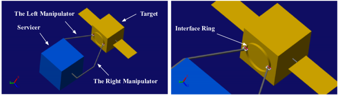
Figure 1: A snapshot of the combined spacecraft

In this paper, the problem of attitude orientation control is considered, i.e., the combined spacecraft is required to realize a commanded desired orientation. Let $\bm{Q}_{\mathrm{d}}=[q_{\mathrm{d}0}~{}\bm{q}_{\mathrm{d}}^{\top}]^{\top}\in{\mathbb{Q}}^{3}$ denote the desired attitude, corresponding to a desired body frame $\mathcal{F}_{\mathrm{D}}$, and $\bm{\omega}_{\mathrm{d}}\in\mathbb{R}^{3}$ the desired angular velocity, respectively. Thus, the attitude error $\bm{Q}_{\mathrm{e}}=[q_{\mathrm{e}0}~{}\bm{q}_{\mathrm{e}}^{\top}]^{\top}$ of $\mathcal{F}_{\mathrm{B}}$ w.r.t. $\mathcal{F}_{\mathrm{D}}$ can be calculated by $\bm{Q}_{\mathrm{e}}=\bm{Q}_{\mathrm{d}}^{*}\otimes\bm{Q}$, where $\bm{Q}_{\mathrm{d}}^{*}=[q_{\mathrm{d}0}~{}-\!\bm{q}_{\mathrm{d}}^{\top}]^{\top}$ denotes the conjugate of $\bm{Q}_{\mathrm{d}}$, and the symbol “$\otimes$” refers to the product operator for any two quaternions $\bm{Q}_{i}=[q_{i0}~{}\bm{q}_{i}^{\top}]^{\top}$ and $\bm{Q}_{j}=[q_{j0}~{}\bm{q}_{j}^{\top}]^{\top}$:

$$\bm{Q}_{i}\otimes\bm{Q}_{j}=\left[\begin{array}[]{c}q_{i0}q_{j0}-\bm{q}_{i}^{\top}\bm{q}_{j}\\ q_{i0}\bm{q}_{j}+q_{j0}\bm{q}_{i}+\bm{q}_{i}^{\times}\bm{q}_{j}\end{array}\right].$$

The attitude error kinematics can be derived as:

$$\dot{\bm{q}}_{\mathrm{e}}=\frac{1}{2}(q_{\mathrm{e}0}\bm{I}_{3}+\bm{q}_{\mathrm{e}}^{\times})\bm{\omega}_{\mathrm{e}},\quad\dot{q}_{\mathrm{e}0}=-\frac{1}{2}\bm{q}_{\mathrm{e}}^{\top}\bm{\omega}_{\mathrm{e}}$$ (2)

where $\bm{\omega}_{\mathrm{e}}=\bm{\omega}-\bm{C}(\bm{Q}_{\mathrm{e}})\bm{\omega}_{\mathrm{d}}$, and the rotation matrix is $\bm{C}(\bm{Q}_{\mathrm{e}})=\bm{I}_{3}-2q_{\mathrm{e}0}\bm{q}_{\mathrm{e}}^{\times}+2\bm{q}_{\mathrm{e}}^{\times}\bm{q}_{\mathrm{e}}^{\times}$. Because the problem of set point control of the attitude is studied in this paper, the desired angular velocity is set as $\bm{\omega}_{\mathrm{d}}=\mathbf{0}$, giving $\bm{\omega}_{\mathrm{e}}=\bm{\omega}$. Hence, the attitude error kinematics (2) can be written as:

$$\dot{\bm{q}}_{\mathrm{e}}=\frac{1}{2}(q_{\mathrm{e}0}\bm{I}_{3}+\bm{q}_{\mathrm{e}}^{\times})\bm{\omega},\quad\dot{q}_{\mathrm{e}0}=-\frac{1}{2}\bm{q}_{\mathrm{e}}^{\top}\bm{\omega}.$$ (3)

Furthermore, the attitude dynamics are given by:

$$\bm{J}_{\mathrm{c}}\dot{\bm{\omega}}=-\bm{\omega}^{\times}\bm{J}_{\mathrm{c}}\bm{\omega}+\bm{u}+\bm{\tau}_{\mathrm{d}},$$ (4)

where $\bm{J}_{\mathrm{c}}\in\mathbb{R}^{3\times 3}$ is the positive-definite symmetric inertia matrix, $\bm{u}\in\mathbb{R}^{3}$ is the control torque, while $\bm{\tau}_{\mathrm{d}}\in\mathbb{R}^{3}$ is an external torque expressed in $\mathcal{F}_{\mathrm{B}}$ representing time-varying disturbances. Note that $\bm{\tau}_{\mathrm{d}}$ can be seen as a collection of additional unconsidered dynamics such as manipulator arm dynamics, rotating solar panels, solar pressure, gravity gradient, etc. Obviously, if $\bm{\tau}_{\mathrm{d}}=\bm{0}$ and $\bm{J}_{\mathrm{c}}$ is accurately known or identified, global asymptotic stability can be easily guaranteed by model-based control, ensuring that the closed-loop trajectory $(\bm{Q}_{\mathrm{e}},\bm{\omega})$ converges to the stable equilibrium $(\bm{1},\bm{0})$.

However, the true value of $\bm{J}_{\mathrm{c}}$ is hard to determine accurately by online parameter identification when the servicer is executing an OOS mission, particularly under maneuvering capability of the target. Similarly, $\bm{\tau}_{\mathrm{d}}$ can be partly reconstructed by space environment models, but some residual uncertainties always remain.

To be able to express some known baseline dynamics w.r.t. the real dynamics of the spacecraft, introduce $\bm{J}_{\mathrm{c}}={\bm{J}}_{\mathrm{c}0}+\tilde{\bm{J}_{\mathrm{c}}}$, where ${\bm{J}}_{\mathrm{c}0}\in\mathbb{R}^{3\times 3}$ represents the nonsingular symmetric nominal inertia matrix of the combined spacecraft, and $\tilde{\bm{J}_{\mathrm{c}}}\in\mathbb{R}^{3\times 3}$ denotes the inertia deviation resulting from the capture and non-nominal characteristics of the target. The inverse of $\bm{J}_{\mathrm{c}}$ can be computed as:

$$\bm{J}_{\mathrm{c}}^{-1}={\bm{J}}_{\mathrm{c}0}^{-1}+\tilde{\bm{J}_{\mathrm{c}}}^{*}$$ (5)

where $\tilde{\bm{J}}_{\mathrm{c}}^{*}=-(\bm{I}_{3}+\bm{J}_{\mathrm{c}0}^{-1}\tilde{\bm{J}}_{\mathrm{c}})^{-1}\bm{J}_{\mathrm{c}0}^{-1}\tilde{\bm{J}}_{\mathrm{c}}\bm{J}_{\mathrm{c}0}^{-1}$.

Thus, the attitude error dynamics of combined spacecraft with uncertainties can be fomulated as

$$\left\{\begin{array}[]{ll}\dot{\bm{q}}_{\mathrm{e}}&=\frac{1}{2}(q_{\mathrm{e}0}\bm{I}_{3}+\bm{q}_{\mathrm{e}}^{\times})\bm{\omega}\\ \dot{\bm{\omega}}&=-\bm{J}_{\mathrm{c}0}^{-1}\bm{\omega}^{\times}\bm{J}_{\mathrm{c}0}\bm{\omega}+\bm{J}_{\mathrm{c}0}^{-1}\bm{u}+\bm{J}_{\mathrm{c}0}^{-1}\bm{d}(\bm{\omega},\bm{u})\end{array}\right.$$ (6)

where $\bm{d}(\bm{\omega},\bm{u})=-\bm{J}_{\mathrm{c}0}\tilde{\bm{J}}_{\mathrm{c}}^{*}(\bm{\omega}^{\times}\bm{J}_{\mathrm{c}0}\bm{\omega})-\bm{\omega}^{\times}\tilde{\bm{J}}_{\mathrm{c}}^{*}\bm{\omega}-\bm{J}_{\mathrm{c}0}\tilde{\bm{J}}_{\mathrm{c}}^{*}\bm{\omega}^{\times}\tilde{\bm{J}}_{\mathrm{c}}^{*}\bm{\omega}+\bm{J}_{\mathrm{c}0}\tilde{\bm{J}}_{\mathrm{c}}^{*}\bm{u}+(\bm{I}_{3}+\bm{J}_{\mathrm{c}0}\tilde{\bm{J}}_{\mathrm{c}}^{*})\bm{\tau}_{\mathrm{d}}$. The dynamic model can be written in a compact form:

$$\dot{\bm{x}}=\underbrace{\bm{f}(\bm{x},\bm{u})}_{{\text{nominal model}}}~{}+~{}\bm{B}\!\underbrace{\breve{\bm{\Delta}}(\bm{x},\bm{u})}_{\text{unknown model}}$$ (7)

where $\bm{x}=\mathrm{vec}(\bm{q}_{\mathrm{e}},\bm{\omega})\in\mathbb{R}^{6}$ is the state vector of the combined spacecraft, $\bm{B}=[\mathbf{0}_{3\times 3}~{}\bm{I}_{3}]^{\top}\in\mathbb{R}^{6\times 3}$ is a projection matrix, $\bm{f}(\bm{x},\bm{u})$ denotes the known, nominal part of the dynamics which has the following form:

$$\bm{f}(\bm{x},\bm{u})=\left[\begin{array}[]{c}\frac{1}{2}(q_{\mathrm{e}0}\bm{I}_{3}+\bm{q}_{\mathrm{e}}^{\times})\bm{\omega}\\ -\bm{J}_{\mathrm{c}0}^{-1}\bm{\omega}^{\times}\bm{J}_{\mathrm{c}0}\bm{\omega}+\bm{J}_{\mathrm{c}0}^{-1}\bm{u}\end{array}\right]\in\mathbb{R}^{6}.$$ (8)

The state and control-dependent unknown model $\breve{\bm{\Delta}}(\bm{x},\bm{u})=\bm{J}_{\mathrm{c}0}^{-1}\bm{d}(\bm{\omega},\bm{u})\in\mathbb{R}^{3}$ includes the model uncertainties and the reactive attitude maneuvering torque of the target. Note that $\breve{\bm{\Delta}}$ also implicitly depends on $t$ because it contains the time-varying external disturbance $\bm{\tau}_{\mathrm{d}}(t)$. In order to be able to design a controller, the system is required to satisfy the following non-restrictive conditions:

Condition 1

There exists known and bounded constants $\lambda_{J}$, $\lambda_{c}>0$, such that the nominal part of the inertia matrix satisfies $\lambda_{\rm{max}}(\bm{J}_{\mathrm{c}0})\leq\lambda_{J}$ and $\lambda_{\rm{min}}(\bm{J}_{\mathrm{c}0})\geq\lambda_{c}$.

Condition 2

The unknown function $\breve{\bm{\Delta}}$ is globally bounded.

The combined spacecraft performs as a “black box” data-generating system, i.e., only input and output data is available from it, just in case of a real spacecraft.

Assumption 1

Measurements of the state (sampling of $\bm{x}(t)$) are obtained online under the sampling time $T_{\mathrm{s}}\in\mathbb{R}^{+}$. The sampling provided value of the states is denoted as $\bm{q}_{\mathrm{e}}[k]:=\bm{q}_{\mathrm{e}}(kT_{\mathrm{s}})$, $\bm{\omega}[k]:=\bm{\omega}(kT_{\mathrm{s}})$, and $\bm{x}[k]:=\bm{x}(kT_{\mathrm{s}})$. Also, we assume that an approximation of the state derivatives $\dot{\bm{x}}[k]$ can be obtained by numerical differentiation. The approximation error can be considered as being part of the measurement noise. Additionally, the control input $\bm{u}$ is generated via ideal zero-order-hold (ZOH) actuation with no delay and synchronized with the sampling, which means that the discrete control signal will be kept constant until the next sampling moment:

$$\bm{u}(t):=\bm{u}[k],~{}\forall t\in(kT_{\mathrm{s}},(k+1)T_{\mathrm{s}}].$$ (9)

2.2 Control Objectives

The primary goal of this paper is to design an adaptive online learning attitude takeover control strategy for the combined spacecraft in the presence of unknown dynamics and attitude maneuverability of the target, such that the attitude of the combined spacecraft follows the desired orientation $\bm{Q}_{\mathrm{d}}$, while the attitude error $\bm{Q}_{\mathrm{e}}$ and the angular velocity $\bm{\omega}$ are ultimately uniformly bounded, and converge to a small set containing the origin.

3 Gaussian Process for Online Model Learning

To achieve the aforementioned control objectives, in this section, our goal is to construct a data-driven and probabilistic model ${\bm{\Delta}}$ of the unknown dynamics $\breve{\bm{\Delta}}$ from previously collected measurement data, and improve the accuracy of the regressed model gradually as more data becomes available and track possible time variation of $\breve{\bm{\Delta}}$.

3.1 Gaussian Process Regression

GP regression (GPR) is a powerful non-parametric framework for learning nonlinear functions from data, where the GP itself can be seen as a distribution over functions [21]. The main advantage of GPR is that it not only provides the estimated mean of the unknown function, but also its variance, which implies the regression accuracy, namely, the model confidence. To approximate the unknown function $\breve{\bm{\Delta}}$, we consider $\bm{\Delta}(\tilde{\bm{x}})$ as a GP which is trained based on the following data set consisting of $N$ collected sampled measurements:

$$\mathcal{D}_{N}=\{{\bm{y}[i]},~{}{\tilde{\bm{x}}[i]}\}_{i=1}^{N}$$ (10)

where the state-input pairs ${\tilde{\bm{x}}[k]}=\mathrm{vec}({\bm{x}[k]},{\bm{u}[k]})\in\mathbb{R}^{9}$ and ${\bm{y}[k]}=\breve{\bm{\Delta}}({\tilde{\bm{x}}[k]})+{\bm{\epsilon}[k]}\triangleq\dot{\bm{x}}[k]-\bm{f}({\bm{x}[k]}),{\bm{u}[k]})+{\bm{\epsilon}[k]}$ denote the training inputs and outputs, respectively, and ${\bm{\epsilon}[k]}$ represents the independent and identically distributed (i.i.d.) measurement noise with ${\bm{\epsilon}[k]}\sim\mathcal{N}(\mathbf{0},{\sigma}^{2}_{\mathrm{\epsilon}}\bm{I})$ and additional approximation error resulting from numerical differentiation.

A vectorial Gaussian process $\mathcal{GP}:\mathbb{R}^{9}\to\mathbb{R}^{3}$ assigns to every point $\bm{\tilde{x}}\in\mathbb{R}^{9}$ a random variable $\mathcal{GP}(\bm{\tilde{x}})$ taking values in $\mathbb{R}^{3}$ such that, for any finite set $\{{\tilde{\bm{x}}[\tau]}\}_{\tau=1}^{N}\subset\mathbb{R}^{3}$, the joint probability distribution of $\mathcal{GP}\left({\tilde{\bm{x}}[1]}\right),\ldots,\mathcal{GP}\left({\tilde{\bm{x}}[N]}\right)$ is multi-dimensional Gaussian. This constitutes a prior distribution over functions, which is denoted by:

$$\bm{\Delta}(\bm{\tilde{x}})\sim\mathcal{GP}(\bm{\mu}(\bm{\tilde{x}}),~{}\bm{\kappa}(\bm{\tilde{x}},\bm{\tilde{x}}^{\prime})),$$ (11)

where $\bm{\mu}(\bm{\tilde{x}})$ is the mean function and $\bm{\kappa}\left(\tilde{\bm{x}},\tilde{\bm{x}}^{\prime}\right)\triangleq\operatorname{cov}\left(\bm{\Delta}(\tilde{\bm{x}}),\bm{\Delta}\left(\tilde{\bm{x}}^{\prime}\right)\right)$ is the positive semi-definite covariance function which corresponds to a measure of correlation of any two data points $(\tilde{\bm{x}},\tilde{\bm{x}}^{\prime})$. Furthermore, the GP model is usually implemented for each dimension of the GP output separately, i.e. in terms of scalar-valued ${\Delta}_{j}(\bm{\tilde{x}})\sim\mathcal{GP}({\mu}_{j}(\bm{\tilde{x}}),~{}{\kappa}_{j}(\bm{\tilde{x}},\bm{\tilde{x}}^{\prime}))$ which approximates the corresponding $\breve{\Delta}_{j}$ with ${j\in\mathbb{I}_{1}^{3}}$. The structure of the multi-dimensional GP is illustrated in Fig. 2, where the outputs are assumed to be uncorrelated, i.e., $\breve{\Delta}_{j}$ is mutually independent, resulting in the choice of $\bm{\kappa}=\mathrm{diag}(\kappa_{1},\kappa_{2},\kappa_{3})$. It should be noted that this assumption is commonly used in GP-based control approaches and it is mild for a real spacecraft task. In this paper, the kernel function is chosen from the exponential family, i.e., the Squared Exponential Automatic Relevance Determination (SEARD) is taken as a prior due to its universal approximation capability:

$$\kappa_{j}\left(\bm{\tilde{x}},\bm{\tilde{x}}^{\prime}\right)\!=\!\sigma_{{\rm{f}},j}^{2}\exp\left(-\frac{1}{2}(\bm{\tilde{x}}-\bm{\tilde{x}}^{\prime})^{\top}\bm{\Lambda}_{j}^{-1}(\bm{\tilde{x}}-\bm{\tilde{x}}^{\prime})\right)$$ (12)

where the diagonal matrix $\bm{\Lambda}_{j}=\mathrm{diag}(\lambda_{j,1}^{2},\ldots,\lambda_{j,9}^{2})$ and $\sigma_{{\rm{f}},j}^{2}\in\mathbb{R}^{+}$ are the length-scale hyperparameters and signal variance, respectively. In order to be able to capture the unknown function $\breve{\bm{\Delta}}$ using the chosen kernel defined GP (11), the following condition is required to be satisfied:

Condition 3

Each ${{\breve{{\Delta}}}_{j}}$ has a bounded reproducing kernel Hilbert Space (RKHS) norm w.r.t. the chosen kernel ${\kappa}_{j}(\bm{\tilde{x}},\bm{\tilde{x}}^{\prime})$, that is, $\|{{\breve{{\Delta}}}_{j}}\|_{\mathcal{H}}<\infty$.

Remark 1

The RKHS norm of ${\breve{{\Delta}}}_{j}$ can be interpreted as a quantitative assessment of the function smoothness, indicating that the function is “well-behaved” w.r.t. the selected kernel.

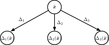
Figure 2: Illustration of the multi-dimensional GP structure.

According to the training data set (10), we define $\tilde{\bm{X}}={\rm{vec}}({\tilde{\bm{x}}[1]},\ldots,{\tilde{\bm{x}}[N]})$ and $\bm{Y}_{j}={\rm{vec}}\left({\bm{y}_{j}[1]},\ldots,{\bm{y}_{j}[N]}\right)$ for $j\in\mathbb{I}_{1}^{3}$. The Gaussian prior for the function $\bm{\Delta}$ and the model likelihood of $\mathcal{D}_{N}$ is denoted as:

$$\mathbb{P}(\bm{\Delta}_{j}) =\mathcal{N}(\bm{\Delta}_{j}\!\mid\!\textbf{0},\bm{K}_{N,j})$$ (13a)

$$\mathbb{P}(\bm{Y}_{j}\!\mid\!\bm{\Delta}_{j}) =\mathcal{N}\left(\bm{Y}_{j}\!\mid\!\bm{\Delta}_{j},\sigma^{2}_{\epsilon,j}\bm{I}_{N}\right)$$ (13b)

where the so-called Gram matrix $\bm{K}_{N,j}\in\mathbb{S}^{N\times N}$ represents the symmetric and semi-definite covariance matrix on the training set $\mathcal{D}_{N}$:

$$\bm{K}_{N,j}\!=\!\!\left[\!\begin{array}[]{ccc}\kappa_{j}\left({\tilde{\bm{x}}[1]},{\tilde{\bm{x}}[1]}\right)&\cdots&\kappa_{j}\left({\tilde{\bm{x}}[1]},{\tilde{\bm{x}}[N]}\right)\\ \vdots&\ddots&\vdots\\ \kappa_{j}\left({\tilde{\bm{x}}[N]},{\tilde{\bm{x}}[1]}\right)&\cdots&\kappa_{j}\left({\tilde{\bm{x}}[N]},{\tilde{\bm{x}}[N]}\right)\end{array}\!\right]$$ (14)

and $\bm{\Delta}_{j}={\rm{vec}}(\Delta_{j}({\tilde{\bm{x}}[1]}),\ldots,\Delta_{j}({\tilde{\bm{x}}[N]})$.

According to Bayes’ Theorem, the posterior distribution can be obtained by maximum a posterior (MAP) estimation:

$$\mathbb{P}(\bm{\Delta}_{j}\!\mid\!\bm{Y}_{j})=\frac{\mathbb{P}(\bm{Y}_{j}\!\mid\!\bm{\Delta}_{j})\mathbb{P}(\bm{\Delta}_{j})}{\mathbb{P}(\bm{Y}_{j})}\\ \propto\mathcal{N}\bigr{(}\bm{\Delta}_{j}\!\mid\!\bm{K}_{N,j}\left(\bm{K}_{N,j}+\sigma^{2}_{\epsilon,j}\bm{I}_{N}\right)^{-1}\bm{Y}_{j},\\ \sigma^{2}_{\epsilon,j}\bm{K}_{N,j}\left(\bm{K}_{N,j}+\sigma^{2}_{\epsilon,j}\bm{I}_{N}\right)^{-1}\bigr{)}.$$ (15)

Then, the predictive distribution of $\Delta_{j}({\bm{\tilde{x}}}^{*})$ on a test point ${\bm{\tilde{x}}}^{*}$ can be derived as:

$$\mathbb{P}(\Delta_{j}^{*} \!\mid\!\tilde{\bm{x}}^{*},\mathcal{D}_{N})$$ (16)

$$=\int\mathbb{P}\left(\Delta_{j}^{*}\!\mid\!\tilde{\bm{x}}^{*},\bm{\Delta}_{j},\tilde{\bm{X}}\right)\mathbb{P}(\bm{\Delta}_{j}\!\mid\!\bm{Y}_{j})\mathrm{d}\bm{\Delta}_{j}$$

$$=\mathcal{N}(\mu_{{\Delta},{j}}(\bm{\tilde{x}}^{*}),\sigma^{2}_{{\Delta},{j}}(\bm{\tilde{x}}^{*}))$$

where the first term inside the integral satisfies the joint distribution:

$$\mathbb{P}\left(\Delta_{j}^{*}\!\mid\!\tilde{\bm{x}}^{*},\bm{\Delta}_{j},\tilde{\bm{X}}\right)$$ (17)

$$=\mathcal{N}\left(\Delta_{j}^{*}\!\mid\!\bm{K}_{*N,j}\bm{K}_{N,j}^{-1}\bm{\Delta}_{j},k_{**,j}-\bm{K}_{*N,j}\bm{K}_{N,j}^{-1}\bm{K}_{N*,j}\right).\vspace{0.1cm}$$

Combining  (15), (16) and (17), we can obtain the posterior mean and variance function for each dimension $j$:

$$\mu_{{\Delta},{j}}(\bm{\tilde{x}}^{*}) =\bm{K}_{*N,j}(\bm{K}_{N}^{j}+\sigma_{\epsilon,j}^{2}\bm{I})^{-1}\bm{Y}_{j},$$ (18a)

$$\sigma^{2}_{{\Delta},{j}}(\bm{\tilde{x}}^{*}) ={k}_{**,j}\!-\!\bm{K}_{*N,j}(\bm{K}_{N,j}\!+\!\sigma_{\epsilon,j}^{2}\bm{I})^{-1}\!\bm{K}_{N*,j},$$ (18b)

which gives a predictive vectorial GP with mean and variance:

$$\bm{\mu}_{\Delta}(\bm{\tilde{x}}^{*}) ={\rm{vec}}(\mu_{{\Delta},{1}}(\bm{\tilde{x}}^{*}),\mu_{{\Delta},{2}}(\bm{\tilde{x}}^{*}),\mu_{{\Delta},{3}}(\bm{\tilde{x}}^{*})),$$ (19a)

$$\bm{\Sigma}_{\Delta}(\bm{\tilde{x}}^{*}) =\mathrm{diag}(\sigma^{2}_{{\Delta},{1}}(\bm{\tilde{x}}^{*}),\sigma^{2}_{{\Delta},{2}}(\bm{\tilde{x}}^{*}),\sigma^{2}_{{\Delta},{3}}(\bm{\tilde{x}}^{*})).$$ (19b)

Furthermore, to obtain an optimal choice of the hyperparameters$\bm{\theta}_{j}=\mathrm{vec}(\sigma_{\epsilon,j}^{2},\sigma_{{\rm{f}},j}^{2},\lambda_{j,1},\ldots,\lambda_{j,9})$, the GP model (11) is trained by maximizing the log-likelihood $\mathcal{L}(\bm{\theta}_{j})=\log\mathcal{N}\left(\mathbf{0},~{}\bm{K}_{N,j}+\sigma^{2}_{\epsilon,j}\bm{I}_{N}\right)$ w.r.t. $\bm{\theta}_{j}$ for each dimension $j$:

$$\hat{\bm{\theta}}_{j}\in\arg\max_{\bm{\theta}_{j}}\mathcal{L}(\bm{\theta}_{j}),$$ (20)

which optimization problem can be efficiently solved by a conjugate gradient-based algorithm [35].

3.2 Recursive Online Sparse GP Regression

As we could see in (20), the computational complexity for the conjugate gradient-based algorithm is $\mathcal{O}(N^{3})$ per iteration, which is cubic in terms of the size of the training data set. According to (18a) and (18b), the computational complexity for predictive mean and variance per test case is $\mathcal{O}(N)$ and $\mathcal{O}(N^{2})$, respectively. Thus, the standard GP is not suitable for large training data sets. However, it is essential to collect a large number of data pairs to explore the state space as much as possible and ensure a sufficiently high regression accuracy. Furthermore, the GP model presented in Section III.3.1 is an offline modeling approach, i.e., the trained GP model is kept fixed online and considered to be sufficient to describe the various on-orbit scenarios. Nevertheless, for the combined spacecraft takeover control missions, the unknown part of the dynamics ${\breve{\bm{\Delta}}}$ may be time-varying due to further attitude maneuvers of the target. Therefore, this section proposes a recursive online sparse GP algorithm (denoted by ROSGP), which significantly reduces the computational complexity of the data-driven model learning while making full use of the online streaming data to update the GP model in real time.

3.2.1 Sparse GP with inducing points

As discussed in Section III.3.1, the diagonal assumption for the prior covariance function $\bm{\kappa}$ allows for the training of the predictive distribution independently for each dimension $j$. Thus, for the simplicity of notation, we will drop the indexing for the output dimension $j$.

We will introduce a novel generalization of the original sparse GP with inducing inputs (SPGP) [36] approach in terms of an efficient online update step. For this we first briefly summarize the SPGP method. The main idea of sparse GP is to find a set of inducing inputs $\bm{\tilde{X}}_{\mathrm{u}}=\mathrm{vec}(\bm{\tilde{x}}_{\mathrm{u},1},...,\bm{\tilde{x}}_{\mathrm{u},M})$ corresponding to inducing outputs $\bm{\Delta}_{\mathrm{u}}=\!\mathrm{vec}({\Delta}_{\mathrm{u},1},...,{\Delta}_{\mathrm{u},M})$ of size $M\ll N$. Akins to (13a), the inducing points follow the Gaussian prior distribution:

$$\mathbb{P}(\bm{\Delta}_{\mathrm{u}})=\mathcal{N}(\bm{\Delta}_{\mathrm{u}}\!\mid\!\mathbf{0},\bm{K}_{M})$$ (21)

where $\bm{K}_{M}\in\mathbb{S}^{M\times M}$ denotes the Gram matrix in terms of inducing inputs. According to the fully independent training conditional approximation (FITC), given the GP inputs with (21), the function values $\bm{\Delta}={\rm{vec}}(\Delta({\tilde{\bm{x}}[1]}),\ldots,\Delta({\tilde{\bm{x}}[N]})$ are i.i.d. Then, the model likelihood is

$$\mathbb{P}(\bm{Y}\!\mid\!\tilde{\bm{X}},\bm{\Delta}_{\mathrm{u}},\bm{\tilde{X}}_{\mathrm{u}}) =\prod_{i=1}^{N}\mathbb{P}({\bm{y}[i]}\!\mid\!{\tilde{\bm{x}}[i]},\bm{\Delta}_{\mathrm{u}},\bm{\tilde{X}}_{\mathrm{u}})$$ (22)

$$=\mathcal{N}(\bm{Y}\!\mid\!\bm{K}_{NM}\bm{K}_{M}^{-1}\bm{\Delta}_{\mathrm{u}},\bm{\Gamma}+\sigma_{\epsilon}^{2}\bm{I}_{N})$$

where $[\bm{K}_{MN}]_{i,j}={\kappa}({\bm{\tilde{x}}_{\mathrm{u},i}},{\tilde{\bm{x}}[j]})$ denotes the covariance matrix between $\mathcal{D}_{M}$ and $\mathcal{D}_{N}$, $\bm{Q}_{N}=\bm{K}_{NM}\bm{K}_{M}^{-1}\bm{K}_{MN}$ can be seen as an approximation of $\bm{K}_{N}$, and $\bm{\Gamma}=\mathrm{diag}\left(\bm{K}_{N}-\bm{Q}_{N}\right)\in\mathbb{R}^{N\times N}$ represents the diagonal covariance matrix which obtains its diagonal structure from the independence between $\bm{\Delta}$ and $\bm{\Delta}_{\mathrm{u}}$.

On the basis of the Bayes’s Theorem and the Gaussian prior (21), the approximated posterior distribution is given by the MAP estimate:

$$\mathbb{P}(\bm{\Delta}_{\mathrm{u}} \!\mid\!\bm{Y},\bm{\tilde{X}}_{\mathrm{u}},\tilde{\bm{X}})\propto\mathbb{P}(\bm{Y}\!\mid\!\bm{\Delta}_{\mathrm{u}},\bm{\tilde{X}}_{\mathrm{u}},\tilde{\bm{X}})\mathbb{P}(\bm{\Delta}_{\mathrm{u}})$$ (23)

$$=\mathcal{N}\left(\bm{\Delta}_{\mathrm{u}}\!\mid\!\bm{K}_{NM}\bm{Q}_{M}^{-1}\bm{K}_{MN}(\bm{\Gamma}+\sigma_{\epsilon}^{2}\bm{I}_{N}\right)^{-1}\bm{Y},$$

$$~{}~{}~{}~{}~{}~{}~{}~{}~{}~{}~{}~{}~{}~{}~{}~{}\qquad\qquad\quad\bm{K}_{M}\bm{Q}_{M}^{-1}\bm{K}_{M})$$

where $\bm{Q}_{M}=\bm{K}_{M}+\bm{K}_{MN}(\bm{\Gamma}+\sigma_{\epsilon}^{2}\bm{I}_{N})^{-1}\bm{K}_{NM}$.

Consequently, the associated posterior distribution of ${\Delta}({\bm{\tilde{x}}}^{*})$ at a new test point $\bm{\tilde{x}}^{*}$ is computed by

$$\mathbb{P}(\Delta^{*}| \mathcal{D}_{N},\bm{\tilde{x}}^{*},\bm{\tilde{X}}_{\mathrm{u}})=\mathcal{N}(\mu_{\Delta}(\bm{\tilde{x}}^{*}),\sigma^{2}_{{\Delta}}(\bm{\tilde{x}}^{*}))$$ (24)

with predictive mean and variance as:

$$\mu_{{\Delta}}(\bm{\tilde{x}}^{*}) =\bm{K}_{*M}\bm{Q}_{M}^{-1}\bm{K}_{MN}\left(\bm{\Gamma}+\sigma_{\epsilon}^{2}\bm{I}_{N}\right)^{-1}\bm{Y},$$ (25a)

$$\sigma^{2}_{{\Delta}}(\bm{\tilde{x}}^{*}) =k_{**}-\bm{K}_{*M}\left(\bm{K}_{M}^{-1}-\bm{Q}_{M}^{-1}\right)\bm{K}_{M*}.$$ (25b)

The inducing data points $\mathcal{D}_{M}=\{\bm{\Delta}_{\mathrm{u}},\tilde{\bm{X}}_{\mathrm{u}}\}$ can be seen as additional hyper-parameters and are optimized along with the original GP hyperparameters $\bm{\theta}=\operatorname{vec}\left(\sigma_{\epsilon}^{2},\sigma_{\mathrm{f}}^{2},\lambda_{1},\ldots,\lambda_{9}\right)$ by maximizing the marginal likelihood function, which can be computed by integrating (21) and (22):

$$\mathbb{P}(\bm{Y}) =\int\mathbb{P}(\bm{Y}\!\mid\!\tilde{\bm{X}},\bm{\Delta}_{\mathrm{u}},\bm{\tilde{X}}_{\mathrm{u}})\mathbb{P}(\bm{\Delta}_{\mathrm{u}})\mathrm{d}\bm{\Delta}_{\mathrm{u}}$$ (26)

$$=\mathcal{N}\left(\mathbf{0},\bm{Q}_{N}+\bm{\Gamma}+\sigma_{\epsilon}^{2}\bm{I}_{N}\right).$$

To initialize the optimization, one reliable approach is to pick random points from the original data set $\mathcal{D}_{N}$.

It is worth mentioning that the inverse of $\bm{K}_{N}+\sigma^{2}_{\epsilon}\bm{I}_{N}$ is reduced to the inverse of the diagonal matrix $\bm{\Gamma}+\sigma_{\epsilon}^{2}\bm{I}_{N}$. In the SPGP based on the FITC assumption, the computational load $\mathcal{O}(M^{2}N)$ mainly comes from the matrix multiplication $\bm{K}_{MN}(\bm{\Gamma}+\sigma_{\epsilon}^{2}\bm{I}_{N})^{-1}\bm{K}_{NM}$. Subsequently, for each test point $\bm{\tilde{x}}^{*}$, the computational complexity for corresponding predictive mean and variance is decreased to $\mathcal{O}(M)$ and $\mathcal{O}(M^{2})$, respectively. Moreover, compared to the marginal likelihood of the standard GP, $\bm{Q}_{N}$ is a low-rank approximation of Gram matrix $\bm{K}_{N}$, which reduces the computational complexity from $\mathcal{O}(N^{3})$ to $\mathcal{O}(M^{2}N)$ during the hyperparameter training. Similar to the standard GP, the SPGP model can be trained by maximizing the log form of the likelihood (26) to find the optimal hyperparameters and $\mathcal{D}_{M}$ by means of a conjugate gradient-based algorithm, which has a computational complexity of $\mathcal{O}(M^{2}N+3MN)$ per iteration.

3.2.2 Recursive Online Sparse GP Regression Algorithm

In this subsection, a novel online update strategy for SPGP is proposed, where the offline trained GP model is recursively updated with the online measurement data sampled at the current time moment $k\in\mathbb{N}$.

Equation (25a) can be rewritten into a linear combination of $M$ kernel functions with the current time moment $k$:

$${\mu}_{\Delta,k}(\bm{\tilde{x}})=\sum_{j=1}^{M}\alpha_{j}\kappa(\tilde{\bm{x}}_{\mathrm{u},j},{\tilde{\bm{x}}[k]})=\bm{\alpha}^{\!\top}\![k]\bm{K}_{M{[k]}}$$ (27)

where $\bm{\alpha}[0]=\bm{Q}_{M}^{-1}\bm{K}_{MN}\left(\bm{\Gamma}+\sigma_{\epsilon}^{2}\bm{I}_{N}\right)^{-1}\bm{Y}\in\mathbb{R}^{M}$ is the initial weight vector obtained from offline training and $[\bm{K}_{M{[k]}}]_{j}=\kappa(\tilde{\bm{x}}_{\mathrm{u},j},{\tilde{\bm{x}}[k]})$ is the corresponding kernel slice evaluated at the input $\bm{\tilde{x}}[k]$.

At time moment $k$, consider the data set $\mathcal{D}_{k}$ given in (10). Define a performance index $\mathcal{W}(\bm{\alpha})$ w.r.t. $\bm{\alpha}$ over the extended data set $\mathcal{D}_{k}=\mathcal{D}_{k-1}\cup{({y}[k],\bm{\tilde{x}}[k])}$ which contains $N_{k}$ data pairs:

$$\mathcal{W}(\bm{\alpha})=\sum_{i=1}^{N_{k}}\lambda^{N_{k}-i}\left(y[i]-\bm{\alpha}^{\top}\bm{K}_{Mi}\right)^{2}+\varsigma\lambda^{N_{k}+1}\|\bm{\alpha}\|^{2}$$ (28)

where $[\bm{K}_{Mi}]_{j}=\kappa(\tilde{\bm{x}}_{\mathrm{u},j},{\tilde{\bm{x}}[i]})$, $0<\lambda\leq 1$ is a user-defined parameter, also known as the forgetting factor. The choice of parameter $\varsigma$ will be discussed later in this section. The weight vector ${\bm{\alpha}[k]}$ at step $k$ is taken as the minimizer of (28), i.e.:

$${\bm{\alpha}[k]}=\arg\min_{\bm{\alpha}\in\mathbb{R}^{M}}\mathcal{W}(\bm{\alpha}).$$ (29)

The optimization problem (29) has an analytical solution. Note that

$${\bm{\Phi}[k]}{\bm{\alpha}[k]}{\bm{\rho}[k]}$$ (30)

where

$${\bm{\Phi}[k]} =\sum_{i=1}^{N_{k}}\lambda^{N_{k}-i}\bm{K}_{Mi}\bm{K}_{Mi}^{\top}+\varsigma\lambda^{N_{k}+1}\bm{I}_{M},$$ (31a)

$${\bm{\rho}[k]} =\sum_{i=1}^{N_{k}}\lambda^{N_{k}-i}\bm{K}_{Mi}y[i].$$ (31b)

Next, (31a) and (31b) can be written in a separate form:

$${\bm{\Phi}[k]} =\lambda{\bm{\Phi}[k-1]}+\bm{K}_{M{[k]}}\bm{K}_{M{[k]}}^{\top},$$ (32a)

$${\bm{\rho}[k]} =\lambda{\bm{\rho}[k-1]}+\bm{K}_{M{[k]}}{y}[k].$$ (32b)

Using formula Woodbury’s matrix inverse for (32a), one has:

$$\bm{\Phi}^{-1}[k]=\lambda^{-1}\bm{\Phi}^{-1}[k-1]-\lambda^{-1}{\bm{L}[k]}\bm{K}_{M{[k]}}^{\top}\bm{\Phi}^{-1}[k-1]$$ (33)

where

$${\bm{L}[k]}=\frac{\lambda^{-1}\bm{\Phi}^{-1}[k-1]\bm{K}_{M{[k]}}}{1+\lambda^{-1}\bm{K}_{M{[k]}}^{\top}\bm{\Phi}^{-1}[k-1]\bm{K}_{M{[k]}}}.$$ (34)

For the convenience of notation, we define ${\bm{P}[k]}=\bm{\Phi}^{-1}[k]$. Thus, from (33) and (34), we have:

$${\bm{P}[k]} =\lambda^{-1}{\bm{P}[k-1]}-\lambda^{-1}{\bm{L}[k]}\bm{K}_{M{[k]}}^{\top}{\bm{P}[k-1]},$$ (35a)

$${\bm{L}[k]} ={\bm{P}[k]}\bm{K}_{M{[k]}}.$$ (35b)

Subsequently, combining (30), (32b), (33), and (34), one can derive:

$${\bm{\alpha}[k]}={\bm{\alpha}[k-1]}-{\bm{L}[k]}\bm{K}_{M{[k]}}^{\top}{\bm{\alpha}[k-1]}+{\bm{L}[k]}{y}[k]$$ (36)

Finally, the weight vector ${\bm{\alpha}[k]}$ can be recursively updated by:

$${\bm{\alpha}[k]}={\bm{\alpha}[k-1]}+{\bm{L}[k]}{r}[k]$$ (37)

where ${r}[k]={y}[k]-\bm{\alpha}^{\top}_{j}[k-1]\bm{K}_{M{[k]}}$.

Remark 2

The online update routine starts from the initial weight vector $\bm{\alpha}[0]$ and the initial user-defined matrix $\bm{P}[0]$. $\bm{\alpha}[0]$ can be obtained by offline training of the GP and $\bm{P}[0]$ is usually selected as $\bm{P}[0]=\varsigma^{-1}\bm{I}_{M}$ with $0<\varsigma\leq 1$. The choice of $\varsigma$ is on the basis of the confidence level of the offline trained GP.

Remark 3

It is worth mentioning that, the convergence of the proposed recursive online sparse GP is inherently guaranteed because it minimizes the performance index (28) at each iterative step.

Remark 4

Compared with the existing online GP methods, such as SOGP [25, 27], and the evolving GP in [30, 31], the proposed recursive online sparse GP do not involve any re-optimization of the hyperparameters nor it requires data-dictionary update at every time step, which ensures low online computational cost.

4 GP-based Online Learning Control

Recalling the control objective given in Section II. 2.2, the goal of this paper is to design a GP-based online learning control strategy to ensure that, for a given attitude set point $\bm{Q}_{\mathrm{d}}=[q_{\mathrm{d}0}~{}\bm{q}_{\mathrm{d}}^{\top}]^{\top}\in{\mathbb{Q}}^{3}$, the closed-loop error and velocity states $(\bm{Q}_{\mathrm{e}},\bm{\omega})$ converge to $(\bm{1},\bm{0})$ even under the unknown dynamics and attitude maneuverability of target. Furthermore, the proposed ROSGP algorithm is employed to derive a probabilistic model of $\breve{\bm{\Delta}}(\tilde{\bm{x}})$, which is utilized for feedforward compensation of the unknown function.

4.1 Controller Design

In order to design the controller, we begin by considering the following lemmas and conditions.

Lemma 1

Consider a GP trained on $\mathcal{D}_{N}$ collected from system (7), which satisfies Condition 3. The estimation error $\|\bm{\mu}_{\Delta}(\bm{\tilde{x}})-{\breve{\bm{\Delta}}}(\bm{\tilde{x}})\|$ is bounded for all $\bm{\tilde{x}}$ on the compact set $\Omega\subset\mathbb{R}^{9}$ with probability $(1-\delta)^{3}$:

$$\mathbb{P}\{\forall\bm{\tilde{x}}\!\in\!\Omega,~{}\|\bm{\mu}_{\Delta}(\bm{\tilde{x}})\!-\!{\breve{\bm{\Delta}}}(\bm{\tilde{x}})\|\leq\|\bm{\beta}\|\|\bm{\Sigma}_{\Delta}^{1/2}(\bm{\tilde{x}})\|\}\geq(1-\delta)^{3}$$ (38)

where $\delta\in(0,1)$, $\bm{\beta}=\mathrm{vec}(\beta_{1},\beta_{2},\beta_{3})$ denotes:

$$\beta_{j}=\sqrt{2\|{\breve{\Delta}}_{j}\|_{\mathcal{H}}^{2}+300\gamma_{j}\log^{3}((N+1)/{\delta})},$$ (39)

and $\gamma_{j}=\max\frac{1}{2}\log|{\bm{I}_{N}+\sigma_{\epsilon,j}^{-2}\bm{K}_{N,j}}|$ represents the maximum information gain w.r.t. the kernel $\kappa_{j},\forall j\in\mathbb{I}_{1}^{3}$.

Proof.

See [37, Lemma 2]. This lemma is a vectorial generalization of the scalar case given in [38]. ∎

Proposition 1

Consider a GP recursively trained on the initial data set $\mathcal{D}_{N}$ and online samples obtained during time interval $[0,k]$ from system (7) which satisfies Condition 3. The estimation error $\|\bm{\mu}_{\Delta,k}(\bm{\tilde{x}})-{\breve{\bm{\Delta}}}(\bm{\tilde{x}})\|$ is bounded for all $\bm{\tilde{x}}$ on the compact set $\Omega\subset\mathbb{R}^{9}$ with probability $(1-\delta)^{3}$:

$$\mathbb{P}\{\forall\bm{\tilde{x}}\!\in\!\Omega,~{}\|\bm{\mu}_{\Delta,k}(\bm{\tilde{x}})\!-\!{\breve{\bm{\Delta}}}(\bm{\tilde{x}})\| \leq\|\bm{\beta}\|\|\bm{\Sigma}_{\Delta}^{1/2}(\bm{\tilde{x}})\|\}$$ (40)

$$\geq(1-\delta)^{3}$$

where $\bm{\mu}_{\Delta,k}(\bm{\tilde{x}})$ represents the predictive mean of the recursively updated GP given by (27) at time $k\in\mathbb{N}$.

The proof of Proposition 1 follows the lines of the proof of Lemma 1. Proposition 1 ensures the boundedness of the GP regression error between the true function ${\breve{\bm{\Delta}}}(\bm{\tilde{x}})$ and the recursively updated predictive mean function $\bm{\mu}_{\Delta,k}(\bm{\tilde{x}})$ with a high probability, where the error bound is proportional to the predictive standard deviation [39].

Based on the online adapted GP, we propose the following controller:

$$\bm{u}{[k]}=-\bm{\zeta}_{\mathrm{p}}(\breve{k}_{\mathrm{p}},\bm{\Sigma}_{\Delta}(\tilde{\bm{x}}{[k]}))\bm{q}_{\mathrm{e}}{[k]}-\bm{\zeta}_{\mathrm{d}}(\breve{k}_{\mathrm{d}},\bm{\Sigma}_{\Delta}(\tilde{\bm{x}}{[k]}))\bm{\omega}{[k]}\\ -\bm{J}_{\mathrm{c}0}\bm{\mu}_{\Delta,k}(\tilde{\bm{x}}{[k]})+\bm{\omega}^{\times}{[k]}\bm{J}_{\mathrm{c}0}\bm{\omega}{[k]},$$ (41)

where ${k\in\mathbb{N}}$ is the discrete time and $[\bm{{\mu}}_{\Delta,k}]_{j}=\bm{\alpha}^{\top}_{j}[k]\bm{K}^{j}_{M+}$, ${j\in\mathbb{I}_{1}^{3}}$ is the predictive mean updated at $k$-th step according to the ROSGP algorithm proposed in Section 3.3.2. The functions $\bm{\zeta}_{\mathrm{p}}$ and $\bm{\zeta}_{\mathrm{d}}$ correspond to the feedback gains of the proposed control law, parameterized in terms of $\breve{k}_{\mathrm{p}}\in\mathbb{R}^{n_{\mathrm{p}}}$, $\breve{k}_{\mathrm{d}}\in\mathbb{R}^{n_{\mathrm{d}}}$. These functions are chosen such that the following condition is satisfied:

Condition 4

For given sets $\mathbb{S}_{\ast}\subseteq{\mathbb{S}}^{3\times 3}$ and $\mathbb{K}_{\ast}\subseteq\mathbb{R}$, the symmetric functions $\bm{\zeta}_{\mathrm{p}},\bm{\zeta}_{\mathrm{d}}:\mathbb{S}^{3\times 3}\to\mathbb{S}^{3\times 3}$ are monotone increasing w.r.t. $K$ and bounded in the sense that the minimum $\underline{\zeta}_{\tau}$ of $\sigma_{\mathrm{min}}(\bm{\zeta}_{\tau}(K,\breve{k}_{\tau})$ and the maximum $\bar{\zeta}_{\tau}$ of $\sigma_{\mathrm{min}}(\bm{\zeta}_{\tau}(K,\breve{k}_{\tau})$ exist over $K\in\mathbb{S}_{\ast}$ and $\breve{k}_{\tau}\in\mathbb{K}_{\ast}^{n_{\tau}}$ where $\sigma_{\mathrm{min}}$ and $\sigma_{\mathrm{max}}$ corresponds to the minimum and maximum singular values and $\tau\in\{\mathrm{p},\mathrm{d}\}$. Then

$$\underline{\zeta}_{\mathrm{p}}\|\bm{w}\|^{2} \leq\bm{w}^{\top}\bm{\zeta}_{\mathrm{p}}{(\breve{k}_{\mathrm{p}},K)}\bm{w}\leq\bar{\zeta}_{\mathrm{p}}\|\bm{w}\|^{2}$$

$$\underline{\zeta}_{\mathrm{d}}\|\bm{w}\|^{2} \leq\bm{w}^{\top}\bm{\zeta}_{\mathrm{d}}{(\breve{k}_{\mathrm{d}},K)}\bm{w}\leq\bar{\zeta}_{\mathrm{d}}\|\bm{w}\|^{2}$$

holds for all $\bm{w}\in\mathbb{R}^{3}$.

There is a wide class of $\bm{\zeta}$ functions such that Condition 4 is satisfied. For instance, if ${\mathbb{S}_{\ast}}$ and $K_{\ast}$ are bounded sets, then polynomial functions can be selected for $\bm{\zeta}_{\sigma}$. Otherwise, they can be chosen as saturated functions such as sigmoid or Gauss functions. Furthermore, $\breve{k}_{\mathrm{p}}$ and $\breve{k}_{\mathrm{d}}$ can be seen as tuning parameters that can be adjusted based on practical experience w.r.t. nominal controller design and do not require extensive tuning procedures.

The implementation of the controller is summarized in Algorithm 1.

4.2 Stability Analysis

In order to conduct the stability analysis of the proposed scheme, we take the assumption that $T_{\mathrm{s}}$ is small enough such that $\bm{x}(t)\approx\bm{x}[k]$ for $t\in(kT_{\mathrm{s}},(k+1)T_{\mathrm{s}}]$, which is reasonable in case of $10$-$50$ Hz sampling based attitude control of a satellite. This simplifies our analysis as instead of sampled data related issues we can focus on the interplay between the GP-based adaptive control law and the motion dynamics of the combined spacecraft. For this reason we will treat (41) as a continuous time control law and consider $\bm{\alpha}$ varying continuously with time $t$.

Algorithm 1 GP-based online learning control strategy for attitude takeover tasks

1:Initialization: Choose $\bm{Q}_{0}$, $\bm{Q}_{\mathrm{d}}$, $\bm{\omega}_{0}$, $\breve{k}_{\mathrm{p}}$, $\breve{k}_{\mathrm{d}}$, $\lambda$, $\bm{P}[0]$,  $k=0$, $T_{\mathrm{s}}$, $N$.

2:Offline Training Phase:

3:Generate training data set $\mathcal{D}_{N}$;

4:Train GP model to optimise $\hat{\bm{\theta}}$ and $\bm{\alpha}[0]$.

5:Online Control Phase:

6:for $k=1,2,...,$ do

7:     Observe the current $\tilde{\bm{x}}[k]$ and $\bm{y}[k]$;

8:     Update:

9:      ${\bm{P}[k]}\!\leftarrow\!\lambda^{-1}{\bm{P}[k-1]}\!-\!\lambda^{-1}\!{\bm{L}[k]}\!\bm{K}_{M{[k]}}^{\top}{\bm{P}[k-1]}$

10:      ${\bm{L}[k]}\leftarrow{\bm{P}[k]}\bm{K}_{M{[k]}}$

11:      ${r}[k]\leftarrow{y}[k]-\bm{\alpha}^{\top}[k-1]\bm{K}_{M{[k]}}$

12:      ${\bm{\alpha}[k]}\leftarrow{\bm{\alpha}[k-1]}+{\bm{L}[k]}{r}[k]$

13:     Compute $\bm{\mu}_{\Delta,k}$ and $\bm{\Sigma}_{\Delta}$ with (27) and (25b);

14:     Compute $\bm{u}{[k]}$ using (41);

15:     Apply $\bm{u}(t)\!=\!\bm{u}{[k]}$ on the system for $t\!\in\![kT_{\mathrm{s}},\!(k+1)T_{\mathrm{s}}]$

16:end for

Assume that the true model uncertainty $\breve{\bm{\Delta}}(\tilde{\bm{x}}(t))=\bm{J}_{\mathrm{c}0}^{-1}\bm{d}(\tilde{\bm{x}}(t))$ at time moment $t$ can be parameterized as $\bm{d}(\tilde{\bm{x}}{(t)})=\bm{J}_{\mathrm{c}0}\breve{\bm{\alpha}}^{\top}(t)\bm{K}_{M{(t)}}$, where $\breve{\bm{\alpha}}(t)$ denotes the true value of the weight for time $t$. Define $\tilde{\bm{\alpha}}(t)=\bm{\alpha}(t)-\breve{\bm{\alpha}}(t)$ as the deviation of the weight for the time moment $t$. Substituting the controller (41) into (6) yields the closed-loop system:

$$\bm{J}_{\mathrm{c}0}\dot{\bm{\omega}}{(t)}=-\bm{\zeta}_{\mathrm{p}}(\breve{k}_{\mathrm{p}},\bm{\Sigma}_{\Delta}{(t)})\bm{q}_{\mathrm{e}}{(t)}-\bm{\zeta}_{\mathrm{d}}(\breve{k}_{\mathrm{d}},\bm{\Sigma}_{\Delta}{(t)})\bm{\omega}{(t)}\\ -\bm{J}_{\mathrm{c}0}\tilde{\bm{\alpha}}^{\top}\!(t)\bm{K}_{M{(t)}}.$$ (42)

The following theorem shows boundedness of the closed-loop signals.

Theorem 1

Consider that the combined spacecraft (7) which satisfies Conditions 1-3 and Assumption 1. Under the proposed GP-based learning control law (41), satisfying Condition 4, where the unknown function $\breve{\bm{\Delta}}$ is modeled by a multi-dimensional GP (11) that is recursively online updated according to Algorithm 1, $\bm{Q}_{\mathrm{e}}$, $\bm{\omega}$ and $\tilde{\bm{\alpha}}$ are guaranteed to be ultimately uniformly bounded.

Proof.

Consider the radially unbounded Lyapunov function:

$$V_{0}(t)=\frac{1}{2}\bm{\omega}^{\top}{(t)}\bm{J}_{\mathrm{c}0}\bm{\omega}{(t)}+\int_{t-T_{\mathrm{s}}}^{t}\!\!\tilde{\bm{\alpha}}^{\top}({\tau})\tilde{\bm{\alpha}}({\tau})\mathrm{d}{\tau}.$$ (43)

By differentiating (43) along the system trajectories (42),

$$\dot{V}_{0}(t) =\!\bm{\omega}^{\top}\!{(t)}(-\bm{\zeta}_{\mathrm{p}}(\breve{k}_{\mathrm{p}},\bm{\Sigma}_{\Delta}{(t)})\bm{q}_{\mathrm{e}}{(t)}\!-\!\bm{\zeta}_{\mathrm{d}}(\breve{k}_{\mathrm{d}},\!\bm{\Sigma}_{\Delta}{(t)})\bm{\omega}{(t)}$$

$$~{}~{}-\!\bm{J}_{\mathrm{c}0}\tilde{\bm{\alpha}}^{\!\top}\!(t)\bm{K}_{M{(t)}})\!+\!\tilde{\bm{\alpha}}^{\!\top}\!(t)\tilde{\bm{\alpha}}(t)-\tilde{\bm{\alpha}}^{\!\top}\!(t-T_{\mathrm{s}})\tilde{\bm{\alpha}}(t-T_{\mathrm{s}})$$

$$\leq-\underline{\zeta}_{\mathrm{d}}\|\bm{\omega}{(t)}\|^{2}-\bm{\omega}^{\top}\!\bm{\zeta}_{\mathrm{p}}(\breve{k}_{\mathrm{p}},\bm{\Sigma}_{\Delta}{(t)})\bm{q}_{\mathrm{e}}{(t)}$$

$$~{}~{}-\bm{\omega}^{\!\top}\!{(t)}\bm{J}_{\mathrm{c}0}\tilde{\bm{\alpha}}^{\!\top}\!(t)\bm{K}_{M{(t)}}+\tilde{\bm{\alpha}}^{\!\top}\!(t)\tilde{\bm{\alpha}}(t)$$

$$~{}~{}-\tilde{\bm{\alpha}}^{\!\top}\!(t-T_{\mathrm{s}})\tilde{\bm{\alpha}}(t-T_{\mathrm{s}}).$$ (44)

Furthermore, from (37), we have:

$$\tilde{\bm{\alpha}}(t) =\bm{\alpha}(t-T_{\mathrm{s}})+\bm{L}(t)r(t)-\breve{\bm{\alpha}}(t),$$ (45)

$$=\tilde{\bm{\alpha}}(t-T_{\mathrm{s}})+\bm{L}(t)r(t)+\breve{\bm{\alpha}}(t-T_{\mathrm{s}})-\breve{\bm{\alpha}}(t).$$

Define $\bm{\Psi}{(t)}=\breve{\bm{\alpha}}(t-T_{\mathrm{s}})-\breve{\bm{\alpha}}(t)$ and $\bm{\Theta}{(t)}=\bm{L}(t)r(t)$. Then, it follows that:

$$\tilde{\bm{\alpha}}^{\!\top}\!(t)\tilde{\bm{\alpha}}(t)=\tilde{\bm{\alpha}}^{\!\top}\!(t-T_{\mathrm{s}})\tilde{\bm{\alpha}}(t-T_{\mathrm{s}})+2\tilde{\bm{\alpha}}^{\top}(t-T_{\mathrm{s}})\bm{\Theta}{(t)}\\ +2\tilde{\bm{\alpha}}^{\!\top}\!(t-T_{\mathrm{s}})\bm{\Psi}{(t)}+2\bm{\Theta}^{\!\top}\!{(t)}\bm{\Psi}{(t)}.$$ (46)

Using the special case of Young’s inequality $\bm{x}^{\top}{\bm{y}}\leq\frac{1}{2}\bm{x}^{\top}\bm{x}+\frac{1}{2}\bm{y}^{\top}\bm{y}$, the following inequalities can be derived:

$$2\tilde{\bm{\alpha}}^{\!\top}\!(t-T_{\mathrm{s}})\bm{\Theta}{{(t)}} \leq\|\tilde{\bm{\alpha}}(t-T_{\mathrm{s}})\|^{2}+\|\bm{\Theta}{{(t)}}\|^{2}$$ (47a)

$$2\tilde{\bm{\alpha}}^{\!\top}\!(t-T_{\mathrm{s}})\bm{\Psi}{{(t)}} \leq\|\tilde{\bm{\alpha}}(t-T_{\mathrm{s}})\|^{2}+\|\bm{\Psi}{{(t)}}\|^{2}$$ (47b)

$$-\bm{\omega}^{\!\top}\!{{(t)}}\bm{\zeta}_{\mathrm{p}}(\breve{k}_{\mathrm{p}},\bm{\Sigma}_{\Delta}{{(t)}})\bm{q}_{\mathrm{e}}{{(t)}} \leq\frac{1}{2}\bar{{\zeta}}_{\mathrm{p}}^{2}+\frac{1}{2}\|\bm{\omega}{{(t)}}\|^{2}$$ (47c)

$$-\bm{\omega}^{\!\top}\!{{(t)}}\bm{J}_{\mathrm{c}0}\tilde{\bm{\alpha}}^{\!\top}\!(t)\bm{K}_{M{(t)}} \leq\frac{1}{2}\lambda_{J}^{2}\bar{\sigma}_{\mathrm{f}}^{4}\|\tilde{\bm{\alpha}}(t)\|^{2}+\frac{1}{2}\|\bm{\omega}{{(t)}}\|^{2}$$ (47d)

where $\bar{\sigma}_{\mathrm{f}}=\mathrm{sup}~{}\sigma_{\mathrm{f},j}$, $j\in\mathbb{I}_{1}^{3}$. Substituting the inequalities (47a)-(47d) into (44) leads to:

$$\dot{V}_{0}(t)\leq-(\underline{\zeta}_{\mathrm{d}}-1)\|\bm{\omega}{{(t)}}\|^{2}-\gamma\|\tilde{\bm{\alpha}}(t)\|^{2}+\frac{1}{2}\bar{\zeta}_{\mathrm{p}}^{2}\\ +(\frac{1}{2}\lambda_{J}^{2}\bar{\sigma}_{\mathrm{f}}^{4}+1+\gamma)(3\|\tilde{\bm{\alpha}}(t-T_{\mathrm{s}})\|^{2}+3\|\bm{\Psi}(t)\|^{2}+3\|\bm{\Theta}(t)\|^{2})\\ -\|\tilde{\bm{\alpha}}(t-T_{\mathrm{s}})\|^{2},$$ (48)

where $\gamma$ is a positive constant. Furthermore, according to the definition of $\bm{\Psi}$ and $\bm{\Theta}$, it is reasonable to assume that $\bm{\Psi}$ and $\bm{\Theta}$ are bounded, that is, $\|\bm{\Psi}{(t)}\|\leq\bar{\phi}$ and $\|\bm{\Theta}{(t)}\|\leq\bar{\xi}$. If $\underline{\zeta}_{\mathrm{d}}-1>0$ and $1-3(\frac{1}{2}\lambda_{J}^{2}\bar{\sigma}_{\mathrm{f}}^{4}+1+\gamma)>0$ are satisfied, then the time derivative of $V_{0}$ can be given as:

$$\dot{V}_{0}(t)\leq-\eta\|\bm{\omega}{(t)}\|^{2}-\gamma\|\tilde{\bm{\alpha}}(t)\|^{2}+\varpi$$ (49)

where $\eta=\underline{\zeta}_{\mathrm{d}}-1$, $\varpi=\frac{1}{2}\bar{\zeta}_{\mathrm{p}}^{2}+3(\frac{1}{2}\lambda_{J}^{2}\bar{\sigma}_{\mathrm{f}}^{4}+1+\gamma)(\bar{\phi}^{2}+\bar{\xi}^{2})$. Clearly, equation (49) indicates that $\bm{\omega}{(t)}$ and $\tilde{\bm{\alpha}}(t)$ are ultimately uniformly bounded in the set:

$$\Omega_{0}\!=\!\!\left\{{(\bm{\omega},\tilde{\bm{\alpha}})\in\mathbb{R}^{3}\times\mathbb{R}^{3}}\Big{|}\|\bm{\omega}\|^{2}\leq\frac{\varpi}{\eta},\|\tilde{\bm{\alpha}}\|^{2}\leq\frac{\varpi}{\gamma}\right\}$$ (50)

Furthermore, in view of the natural boundedness of the quaternion, one can conclude that the system state $(\bm{Q}_{\mathrm{e}},\bm{\omega})$ is ultimately uniformly bounded. ∎

Theorem 1 implies the existence of the ultimate bound of system states $(\bm{Q}_{\mathrm{e}},\bm{\omega})$. However, because $\varpi$ is an unknown constant, the specific size of the ultimate bound is hard to know. Next, we will make a step further to quantify the ultimate bound of system states $(\bm{Q}_{\mathrm{e}},\bm{\omega})$ by taking Proposition 1 into consideration.

Theorem 2

Consider that the combined spacecraft (7) which satisfies Conditions 1-3 and Assumption 1. Under the proposed GP-based learning control law (41), satisfying Condition 4 and where the unknown function $\breve{\bm{\Delta}}$ is modeled by a multi-dimensional GP (11) that is recursively online updated according to Algorithm 1, $\bm{Q}_{\mathrm{e}}$ and $\bm{\omega}$ are guaranteed to be ultimately uniformly bounded with a probability of $(1-\delta)^{3}$.

Proof.

Consider the Lyapunov function candidate as:

$$V_{1} =(\bm{\zeta}_{\mathrm{p}}(\breve{k}_{\mathrm{p}},\bm{\Sigma}_{\Delta})+\nu\bm{\zeta}_{\mathrm{d}}(\breve{k}_{\mathrm{d}},\bm{\Sigma}_{\Delta}))((1-q_{\mathrm{e}0})^{2}+\bm{q}_{\mathrm{e}}^{\top}\bm{q}_{\mathrm{e}})$$ (51)

$$~{}~{}+\frac{1}{2}\bm{\omega}^{\top}\bm{J}_{\mathrm{c}0}\bm{\omega}+\nu\bm{q}_{\mathrm{e}}^{\top}\bm{J}_{\mathrm{c}0}\bm{\omega},$$

where $\nu>0$ is a constant. The proof for the positive-definiteness of $V_{1}$ can be found in [40].

By differentiating $V_{1}$ and employing the closed-loop system and controller, one can derive:

$$\dot{V}_{1} =(\bm{\zeta}_{\mathrm{p}}(\breve{k}_{\mathrm{p}},\bm{\Sigma}_{\Delta})+\nu\bm{\zeta}_{\mathrm{d}}(\breve{k}_{\mathrm{d}},\bm{\Sigma}_{\Delta}))\bm{q}_{\mathrm{e}}^{\top}\bm{\omega}$$ (52)

$$\quad+(\bm{\omega}+\nu\bm{q}_{\mathrm{e}})^{\top}(-\bm{\zeta}_{\mathrm{p}}(\breve{k}_{\mathrm{p}},\bm{\Sigma}_{\Delta})\bm{q}_{\mathrm{e}}-\bm{\zeta}_{\mathrm{d}}(\breve{k}_{\mathrm{d}},\bm{\Sigma}_{\Delta})\bm{\omega}$$

$$\quad-\bm{J}_{\mathrm{c}0}\bm{\mu}_{\Delta,k}(\tilde{\bm{x}})+\bm{d}(\tilde{\bm{x}}))+\frac{1}{2}\nu\bm{\omega}^{\top}(q_{\mathrm{e}0}\bm{I}_{3}+\bm{q}_{\mathrm{e}}^{\times})\bm{J}_{\mathrm{c}0}\bm{\omega}$$

According to Cauchy-Schwartz inequality and $\|q_{\mathrm{e}0}\bm{I}_{3}+\bm{q}_{\mathrm{e}}^{\times}\|=1$:

$$\dot{V}_{1} =-\nu\bm{\zeta}_{\mathrm{p}}(\breve{k}_{\mathrm{p}},\bm{\Sigma}_{\Delta})\|\bm{q}_{\mathrm{e}}\|^{2}-\bm{\zeta}_{\mathrm{d}}(\breve{k}_{\mathrm{d}},\bm{\Sigma}_{\Delta})\|\bm{\omega}\|^{2}$$ (53)

$$~{}~{}~{}+\frac{1}{2}\nu\bm{\omega}^{\top}(q_{\mathrm{e}0}\bm{I}_{3}+\bm{q}_{\mathrm{e}}^{\times})\bm{J}_{\mathrm{c}0}\bm{\omega}$$

$$\quad+(\bm{\omega}+\nu\bm{q}_{\mathrm{e}})^{\top}(\bm{d}(\tilde{\bm{x}})-\bm{J}_{\mathrm{c}0}\bm{\mu}_{\Delta,k}(\tilde{\bm{x}}))$$

$$\leq-\nu\underline{\zeta}_{\mathrm{p}}\|\bm{q}_{\mathrm{e}}\|^{2}-\lambda_{J}(\underline{\zeta}_{\mathrm{d}}-\frac{1}{2}\nu)\|\bm{\omega}\|^{2}$$

$$~{}~{}~{}+(\bm{\omega}+\nu\bm{q}_{\mathrm{e}})^{\top}(\bm{d}(\tilde{\bm{x}})-\bm{J}_{\mathrm{c}0}\bm{\mu}_{\Delta,k}(\tilde{\bm{x}}))$$

Further combining Proposition 1 with (53), it can be deduced that:

$$\mathbb{P}\{\dot{V}_{1} \leq-\lambda_{\rm{min}}(\bm{M}_{l})\|\bm{x}\|^{2}+\lambda_{J}(\|\bm{\omega}\|+\nu\|\bm{q}_{\mathrm{e}}\|)\|\bm{\beta}\|\|\bm{\Sigma}^{1/2}_{\Delta}\|\}$$ (54)

$$\qquad\qquad\qquad\geq(1-\delta)^{3}$$

holds for all $t\in\mathbb{R}_{0}^{+}$ where

$$\bm{M}_{l}=\left[\begin{array}[]{cc}\nu\underline{\zeta}_{\mathrm{p}}&0\\ 0&\underline{\zeta}_{\mathrm{d}}-\frac{1}{2}\nu\lambda_{J}\end{array}\right].$$ (55)

From the definition of ${V}_{1}$, we have:

$${V}_{1}\leq\bm{x}^{\top}\bm{M}_{s}\bm{x}\leq\lambda_{\rm{max}}(\bm{M}_{s})\|\bm{x}\|^{2},$$ (56)

$$\quad\bm{M}_{s}=\left[\begin{array}[]{cc}2(\bar{\zeta}_{\mathrm{p}}+\nu\bar{\zeta}_{\mathrm{d}})&\frac{1}{2}\nu\lambda_{J}\\ \frac{1}{2}\nu\lambda_{J}&\frac{1}{2}\lambda_{J}\end{array}\right]$$

Moreover, we can derive the boundedness of $\bm{q}_{\mathrm{e}}$ and $\bm{\omega}$, which indicates that:

$$\|\bm{q}_{\mathrm{e}}\|\leq\sqrt{\frac{{V}_{1}}{\bar{\zeta}_{\mathrm{p}}+\nu\bar{\zeta}_{\mathrm{d}}}},\quad\|\bm{\omega}\|\leq\sqrt{\frac{2{V}_{1}}{\lambda_{c}}}.$$ (57)

Consequently, from (54), (56) and (57), one can readily derive:

$$\mathbb{P}\bigg{\{}\dot{V}_{1}\leq-\frac{\lambda_{\rm{min}}(\bm{M}_{l})}{\lambda_{\rm{max}}(\bm{M}_{s})}{V}_{1}\\ +\lambda_{J}\left(\sqrt{\frac{2{V}_{1}}{\lambda_{c}}}+\nu\sqrt{\frac{{V}_{1}}{\bar{\zeta}_{\mathrm{p}}+\nu\bar{\zeta}_{\mathrm{d}}}}\right)\varepsilon\bigg{\}}\geq(1-\delta)^{3},$$ (58)

holds for all $t\in\mathbb{R}_{0}^{+}$ where $\varepsilon\geq\|\bm{\beta}\|\|\bm{\Sigma}_{\Delta}^{1/2}\|$.

Next, we will take a step further to estimate the ultimately uniform bound for attitude error $\bm{q}_{\mathrm{e}}$ and angular velocity $\bm{\omega}$. Defining $W=\sqrt{V_{1}}$, we have that $\dot{W}=\dot{{V}}_{1}/(2\sqrt{{V}_{1}})$ holds when $V_{1}\not=0$, that is:

$$\mathbb{P}\left\{\dot{W}\leq-\frac{\lambda_{\rm{min}}(\bm{M}_{l})}{2\lambda_{\rm{max}}(\bm{M}_{s})}{W}+\frac{\lambda_{J}\varepsilon}{\sqrt{2}}\vartheta\right\}\geq(1-\delta)^{3}$$ (59)

with $\vartheta=\left(\sqrt{\frac{1}{2\lambda_{c}}}+\nu\sqrt{\frac{1}{2(\bar{\zeta}_{\mathrm{p}}+\nu\bar{\zeta}_{\mathrm{d}})}}\right)$. Integrating the inequality in (59) leads to:

$$0\leq\sqrt{V_{1}(t)}\leq\left(\sqrt{V_{1}(0)}-s_{1}\right)e^{-s_{2}t}+s_{1}$$ (60)

where

$$s_{1}=\frac{\sqrt{2}\lambda_{J}\varepsilon\vartheta\lambda_{\rm{max}}(\bm{M}_{s})}{\lambda_{\rm{min}}(\bm{M}_{l})},\quad s_{2}=\frac{\lambda_{\rm{min}}(\bm{M}_{l})}{2\lambda_{\rm{max}}(\bm{M}_{s})}.$$

Thus, when $t\to\infty$, one can derive:

$$\lim_{t\to\infty}\sup\sqrt{V_{1}(t)}\leq s_{1}$$ (61)

Recalling (57), we can finally compute the bound of $\bm{q}_{\mathrm{e}}$ and $\bm{\omega}$ that:

$$\lim_{t\to\infty}\sup\|\bm{q}_{\mathrm{e}}{(t)}\|=\frac{s_{1}}{\sqrt{\bar{\zeta}_{\mathrm{p}}+\nu\bar{\zeta}_{\mathrm{d}}}},$$ (62a)

$$\lim_{t\to\infty}\sup\|\bm{\omega}{(t)}\|=\sqrt{\frac{2}{\lambda_{c}}}s_{1}.$$ (62b)

Furthermore, due to $2(\bar{\zeta}_{\mathrm{p}}+\nu\bar{\zeta}_{\mathrm{d}})(1-q_{\mathrm{e}0})\leq V_{1}$, we have:

$$\lim_{t\to\infty}\sup\|q_{\mathrm{e}0}{(t)}\| \geq 1-\frac{\lim_{t\to\infty}\sup{V_{1}(t)}}{2(\bar{\zeta}_{\mathrm{p}}+\nu\bar{\zeta}_{\mathrm{d}})}$$

$$\geq 1-\frac{s_{1}^{2}}{2(\bar{\zeta}_{\mathrm{p}}+\nu\bar{\zeta}_{\mathrm{d}})}.$$ (63)

Then,

$$\lim_{t\to\infty}\sup\|\bm{q}_{\mathrm{e}}{(t)}\| =\lim_{t\to\infty}\sup\sqrt{1-q_{\mathrm{e}0}^{2}}$$

$$\leq\sqrt{1-(1-\frac{s_{1}^{2}}{2(\bar{\zeta}_{\mathrm{p}}+\nu\bar{\zeta}_{\mathrm{d}})})^{2}}.$$ (64)

Comparing (64) and (62a), it can be concluded that the upper bound for $\bm{q}_{\mathrm{e}}$ is further reduced. Hence, the system states $\bm{q}_{\mathrm{e}}$ and $\bm{\omega}$ ultimately converge to the compact set $\Omega_{1}$ and $\Omega_{2}$ within the probability $(1-\delta)^{3}$:

$$\Omega_{1} =\left\{\bm{Q}_{\mathrm{e}}\in{\mathbb{Q}}^{3}\ \Big{|}\ \|\bm{q}_{\mathrm{e}}\|\leq\sqrt{1-(1-\frac{s_{1}^{2}}{2(\bar{\zeta}_{\mathrm{p}}+\nu\bar{\zeta}_{\mathrm{d}})})^{2}}\right\}$$

$$\Omega_{2} =\left\{\bm{\omega}\in\mathbb{R}^{3}\ \Big{|}\ \|\bm{\omega}\|\leq\sqrt{\frac{2}{\lambda_{c}}}s_{1}\right\}$$

This completes the proof. ∎

The block diagram of the closed-loop control system is shown in Fig. 3.

Figure 3: Block diagram of the proposed control strategy.

Remark 5

Compared to the existing attitude takeover controllers for the combined spacecraft, such as NN-based compensation [16] and adaptive control in [13], the advantages of the proposed GP-based online learning controller are as follows:

1) As a nonparametric modeling approach, the predictive outputs of GP are inherently probabilistic. The GP variance quantifies the confidence level of the predicted uncertainty, while the mean corresponds to the estimated uncertainty. Both the mean and the variance are incorporated into the control scheme, where the latter effectively improves the robustness of the algorithm. To the best of the authors’ knowledge, existing results for the uncertainty quantification of NN mainly include Monte Carlo methods, dropout, and Bayesian ANNs. These approaches are generally complex and computationally too demanding to be applied in a real implementation on a spacecraft.

2) In contrast to the manual time-consuming tuning process for the hyperparameters of the NN-based adaptive control scheme, the hyperparameters of the GP scheme, such as $\bm{\theta}_{j}=\operatorname{vec}(\sigma_{\epsilon,j}^{2},\sigma_{\mathrm{f},j}^{2},\lambda_{j,1},\ldots,\lambda_{j,9})$, are automatically tuned by marginalized likelihood based optimization, while the remaining parameters of the adaptive feedback controller, such as $\breve{k}_{\mathrm{p}}$ and $\breve{k}_{\mathrm{d}}$, can be designed by practical experience with PD control design for such systems with known nominal inertia matrix $\bm{J}_{\mathrm{c0}}$ and does not require extensive tuning procedures.

3) As a data-driven adaptive approach, the proposed GP-based learning controller only needs an initial “rough” model of the unknown dynamics that is learnt with only a small amount of data and needs no extensive exploration of the entire state space before safe execution of the mission. Subsequently, the initial GP model is updated online as new operational data becomes available to ensure continuous adaption and performance improvement of the controller.

5 Simulation Results

In this section, simulation results under various on-orbit scenarios are presented to illustrate the effectiveness of our proposed control strategy.

5.1 Simulation Platform

A SimMechanics-based, high-fidelity simulator has been developed for the combined spacecraft to accurately characterize its attitude motion under the considered model uncertainties and target maneuvering, and act as the physical system and data-generator for the proposed online learning control strategy. As shown in Fig. 4, the system consists of two components, namely the servicer and the target. The servicer, simplified as a cubesat, is equipped with two robotic arms on each side for capturing the target. Each arm is composed of three segments, and once capture is completed, the joints are locked in a specific configuration. The target is also modeled as a cube with solar panels on both sides and a capture interface in the form of a docking ring. For the simplicity of the study, each component in the system is considered as a rigid body without flexibility.

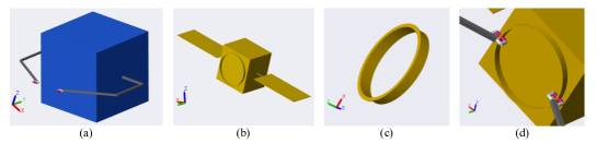
Figure 4: Parts the combined spacecraft assembly: (a) Servicer spacecraft, (b) Target spacecraft, (c) Docking ring on the target, (d) Capture point.

The simulation platform can be seen as a black-box system, i.e. the attitude motion equations in the analytical form are “packaged” within Simulink, and only the I/O ports are used for the proposed adaptive control algorithm, just as it would be the case for a real spacecraft. The physical parameters considered in the simulator are given in Table. 1, which are mainly based on [41]. Note that appropriate modifications have been done to make this scenario more suitable for implementation in Matlab/SimMechanics.

Table 1: Physical parameters of the combined spacecraft

		Parameter	Value
Servicer	Body	Size (m)	$2\times 2\times 2$
		Inertia ($\rm{kg}\cdot m^{2}$)	$\rm{diag}(405,405,405)$
		Mass (kg)	1080
	Robotic Arm	Length per link (m)	0.73, 1, 2
		Mass per link (kg)	6
		Inertia per link ($\rm{kg}\cdot m^{2}$)	$\rm{diag}(0.03,0.73,0.73)$
Target	Body	Size (m)	$2\times 2\times 2$
		Inertia ($\rm{kg}\cdot m^{2}$)	$\rm{diag}(36.8,37.5,36.8)$
		Mass (kg)	75
	Others	Size of solar panels (m)	$1.5\times 0.8\times 0.01$
		Size of docking ring (m)	0.423/0.443 (I/O)

The studied simulation scenario is as follows. The target is a partially malfunctioning satellite working in a sun-oriented mode. Thus, after being captured by the servicer, the target attempts to perform active attitude maneuvers throughout the takeover task, i.e., when the servicer applies a control torque to the target that leads to a deviation from its initial attitude orientation, the target will generate a competitive torque against the control torque to keep its attitude. The unknown model uncertainties considered in this example consist of two parts, the unknown dynamics corresponding to additional robot arms, flexible solar panels, etc., and the additional dynamics caused by the target-generated torque. The active attitude control law for the target is chosen to be of the PD form:

$$\bm{u}_{\mathrm{t}}=-\bm{K}_{\mathrm{pt}}\bm{q}_{\mathrm{et}}-\bm{K}_{\mathrm{dt}}\bm{\omega}_{\mathrm{t}}$$ (65)

where the subscript “t” denotes the target-related variables, $\bm{K}_{\mathrm{pt}}=0.02\bm{J}_{\mathrm{t}}$, $\bm{K}_{\mathrm{dt}}=0.05\bm{J}_{\mathrm{t}}$, $\bm{q}_{\mathrm{et}}=\bm{q}_{\mathrm{dt}}^{-1}\otimes\bm{q}_{\mathrm{t}}$, $\bm{q}_{\mathrm{dt}}$ is the vector part of initial quaternion of the target relative to the inertial coordinate system $\mathcal{F}_{\mathrm{I}}$. Note that (65) is part of the black-box simulation system and it is not known by the servicer.

5.2 Adaptive Control Under Unknown Model Uncertainties

After docking, the initial Euler angle for the combined spacecraft is $[15~{}5~{}-20]^{\circ}$, and the initial angular velocity is $\bm{\omega}_{0}=[0.01~{}0.02~{}-0.01]^{\top}$ rad/s. In this simulation scenario, the attitude orientation of the combined spacecraft is forced to converge to $\bm{Q}_{\mathrm{d}}=[1~{}0~{}0~{}0]^{\top}$, which corresponds to an attitude stabilization task. Generally, there are two options to construct the training data set $\mathcal{D}_{N}$: Either just using the transient data of the closed-loop system or applying excitation torque on the spacecraft. In this paper, only the transient data regarding orientation change with a baseline PD controller is collected, which represents a low-profile scenario. That is, the training data is collected during the control process in the first 50s of the simulation. With a sampling frequency of 10 Hz, the size of the collected training set is $N=500$. Considering the sensor-based measurement of $\bm{q}_{\mathrm{e}}$ and $\bm{\omega}$, the training outputs are corrupted by a Gaussian white noise $\epsilon[k]$ with $\epsilon[k]\sim\mathcal{N}(0,0.05)$. The feedback gain for the baseline controller follows $\bm{K}_{\mathrm{p0}}=0.1\bm{J}_{\mathrm{c}0}$, $\bm{K}_{\mathrm{d0}}=0.3\bm{J}_{\mathrm{c}0}$, where the nominal inertia matrix of the combined spacecraft is selected as $\bm{J}_{\mathrm{c}0}=\rm{diag}(600,450,600)~{}kg\cdot m^{2}$. It is worth mentioning that the value of $\bm{J}_{\mathrm{c}0}$ is simply selected based on the known inertia matrix of the servicer.

For the obtained data set $\mathcal{D}_{N}$, both a sparse and a standard GP are trained, of which the hyperparameters of both are optimized by the conjugated gradient descent algorithm. Specifically, in the case of ROSGP, the inducing points are initialized randomly inside $\mathcal{D}_{N}$ with the size of $M=50$ and the initial $\bm{\alpha}[0]$ is computed according to (25a). The initial value of $\bm{P}$ is set to $\bm{P}[0]=10^{2}\bm{I}_{M}$. Then, at $t=50$s, the controller is updated to (41) where the recursive update routine is activated. The feedback gain functions $\bm{\zeta}_{\mathrm{p}}(\breve{k}_{\mathrm{p}},\bm{\Sigma}_{\Delta})$ and $\bm{\zeta}_{\mathrm{d}}(\breve{k}_{\mathrm{d}},\bm{\Sigma}_{\Delta})$ are selected as linear functions of the variance: $\bm{\zeta}_{\mathrm{p}}(\breve{k}_{\mathrm{p}},\bm{\Sigma}_{\Delta})=\bm{J}_{\mathrm{c}0}(\breve{k}_{\mathrm{p}}+0.1{\bm{\Sigma}_{\Delta}^{1/2}})$ and $\bm{\zeta}_{\mathrm{d}}(\breve{k}_{\mathrm{d}},\bm{\Sigma}_{\Delta})=\bm{J}_{\mathrm{c}0}(\breve{k}_{\mathrm{d}}+0.2{\bm{\Sigma}_{\Delta}^{1/2}})$ with $\breve{k}_{\mathrm{p}}=0.02$ and $\breve{k}_{\mathrm{d}}=0.05$. It can be easily verified that $\bm{\zeta}_{\mathrm{p}}(\cdot)$ and $\bm{\zeta}_{\mathrm{d}}(\cdot)$ satisfy Condition 4 because the GP predictive variance is bounded by $\sup k_{**,j}$ for $j\in\mathbb{I}_{1}^{3}$. Furthermore, the selection of parameters $\breve{k}_{\mathrm{p}}$ and $\breve{k}_{\mathrm{d}}$ is based on practical experience with PD control design for such systems with known nominal inertia matrix $\bm{J}_{\mathrm{c0}}$, and does not require extensive tuning procedures.

The proposed recursive online sparse GP-based learning controller is compared to:

• Baseline PD controller: This is the initial controller to generate the training data set during the first 50s, and it is kept fixed after $t=50$s.

• Standard GP-based controller: This controller keeps the same structure and parameters as the proposed controller (41), but it is based only on an initial trained GP without the recursive online update strategy.

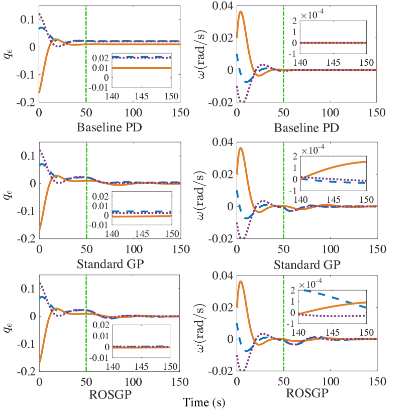
Figure 5: Trajectories of $\bm{q}_{\mathrm{e}}$ and $\bm{\omega}$ under the considered controllers. The lines in each subplot describe the three components of these signals. It can be observed that the ROSGP performs the best in terms of the steady-error of $\bm{q}_{\mathrm{e}}$ due to its capability of online GP compensation, while the baseline PD controller achieves the smallest steady-state error in terms of $\bm{\omega}$ at the expense of high-gain feedback.

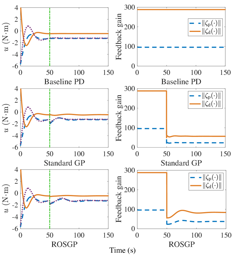
Figure 6: Control inputs $\bm{u}$ and the norm of feedback gain under the considered controllers. It can be observed that the high-gain feedback of the baseline PD controller remains fixed throughout the entire task, while the GP-based controllers can adaptively adjust the feedback gain according to the GP predictive variance, keeping it at a low level while ensuring pointing accuracy.

Figure 7: A Pareto-front-like comparison of the normalized feedback gain and system error between the baseline PD and proposed ROSGP-based controllers. The color indicates the control efforts during the task. It is apparent that at the same level of system error, the ROSGP-based controller requires a relatively small feedback gain.

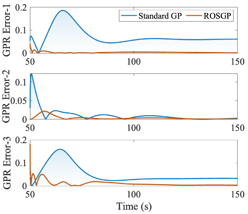
Figure 8: Absolute value of the GP estimation error $\|\mu_{\Delta,j}-\breve{\Delta}_{j}\|$ for each dimension $j$ evaluated over time under the stabilization scenario.

The trajectories of the system states, control inputs, together with the feedback gain are depicted in Figs. 5-6, where the green line indicates that the controller updates at 50s. Simulation results show that all three controllers succeed in achieving the attitude stabilization task for the combined spacecraft. Also, as shown in Fig. 6, the feedback gain of baseline PD remains constant during the entire task, and the two GP-based controllers can adapt its gain with the predictive variance. It is worth mentioning that the ROSGP performs the best in terms of final pointing error, because the unknown function $\breve{\bm{\Delta}}(\tilde{\bm{x}})$ in the combined spacecraft dynamics is real-time compensated by the predictive mean $\bm{\mu}_{\Delta}(\tilde{\bm{x}})$ of the trained GP model and further completed by the ROSGP algorithm with online adaption. However, it is more cautious hence its settling time is slightly slower which can be seen in terms of the slower convergence of the angular velocity. Additionally, while the baseline PD controller remains the largest steady-state error of $\bm{q}_{\mathrm{e}}$ without the GP compensation, it seems to achieve the smallest steady-state error of $\bm{\omega}$, nonetheless, at the expense of high-gain feedback. This can also be seen in Fig.  7, where the Pareto-front-like figure shows the relationship between the normalized feedback gain $\sqrt{\|\bm{\zeta}_{\mathrm{p}}(\cdot)\|^{2}+\|\bm{\zeta}_{\mathrm{d}}(\cdot)\|^{2}}$ and system error $\sqrt{\|\bm{q}_{\mathrm{e}}\|^{2}+\|\bm{\omega}\|^{2}}$ of the two controllers in 30 simulation cases. The color indicates the control efforts $\int_{50}^{150}\|\bm{u}\|\mathrm{d}t$ during the task. It is clear that the proposed ROSGP-based controller requires a relatively modest feedback gain at the same level of system error.

The absolute value of the two GP estimation errors $\|\mu_{\Delta,j}-\breve{\Delta}_{j}\|$ is depicted in Fig. 8. One can see that there exists a significant estimation error between the predictive mean of standard GP and true function due to the initial data set $\mathcal{D}_{N}$ collected in the first 50s is not sufficient to describe the whole state space. In contrast, the model accuracy is adaptively enhanced by the proposed ROSGP, and the full compensation for the unknown function $\breve{\bm{\Delta}}(\tilde{\bm{x}})$ is achieved.

5.3 Adaptive Control Under Re-maneuver Scenario

During the on-orbit takeover control tasks, the combined spacecraft often needs to perform additional new tasks after attitude stabilization, such as maneuvering to a new attitude orientation for awaiting further missions. This new attitude orientation may be far from the initial training data set $\mathcal{D}_{N}$, which poses a significant challenge for the GP-based learning control strategy. Therefore, it is essential to verify the generalization performance and control effectiveness of the proposed GP-based online learning control strategy in untrained areas.

Consider the following scenario: On the basis of the effective attitude stabilization in the first 150s, the combined spacecraft is required to re-maneuver to a new attitude orientation $\bm{Q}_{\mathrm{d}}=[0.899~{}-0.30~{}0.20~{}-0.10]^{\top}$. Meanwhile, to further illustrate the superior performance of the proposed ROSGP-based control strategy, rougher conditions are considered in this scenario. In addition to larger uncertainties resulting from the re-orientation outside the trained area and competitive torque of the target maneuver, large time-varying external disturbances that may result from the movement of an extra robotic arm, fuel sloshing, and flexible vibrations of solar panels, etc., are applied to the combined spacecraft from 150s, and can be modeled as $\bm{\tau}_{\mathrm{d}}(t)=[0.5\sin 0.1t,-\sin 0.15t,1.5\sin(-0.15t+1.5)]^{\top}\rm{N\cdot m}$.

To show the advantages of the proposed GP-based learning control strategy, the NN-based adaptive control scheme (denoted by ANN) in [16] is applied in the considered scenario. In this ANN approach, radial basis functions (RBF) are chosen as the activation functions to estimate and compensate the unknown uncertainties. The NN structure $\hat{\bm{\Delta}}=\hat{\bm{\Theta}}^{\top}\bm{\Phi}_{\rho}$ used to estimate the unknown dynamics $\breve{\bm{\Delta}}$ contains 10 neurons with centers $c_{i}\in\mathbb{R}^{6}$ ($i\in\mathbb{I}_{1}^{10}$) randomly distributed in $[-2,2]^{6}$ and widths $\sigma_{i}=2$. Each element of the initial NN weights $\hat{\bm{\Theta}}(0)$ is chosen between $\pm 0.5$ randomly. The adaptive law for the NN weight is given by: $\dot{\hat{\Theta}}=\bm{F}_{\rho}\Phi_{\rho}\bm{r}^{\top}-k_{\rho}\bm{F}_{\rho}\|\bm{r}\|\hat{\Theta}$ where $\bm{r}=\bm{\omega}+\epsilon\bm{q}_{\mathrm{e}}$. The parameters for the ANN controller are selected as $\bm{F}_{\rho}=200\bm{I}_{3}$, $k_{\rho}=1$, $\bm{\Lambda}=0.1\bm{I}_{3}$, $\epsilon=0.1$. It should be emphasized that the choice of all the aforementioned parameters in the ANN method is required to be tuned manually, for which there are no comprehensive tuning rules. For a fair comparison, the previously used control scenario was used where the GP-based feedforward has been substituted by the ANN compensation term.

Figure 9: Trajectories of $\bm{q}_{\mathrm{e}}$ and $\bm{\omega}$ under the considered controllers and additional torque disturbances. Due to the torque disturbances, only ROSGP can achieve reasonably low steady-state error.

Figure 10: Control inputs $\bm{u}$ and the norm of the feedback gain under the considered controllers. One can observe that the feedback gain of GP-based controllers can vary according to the predictive variance of GP in the untrained areas.

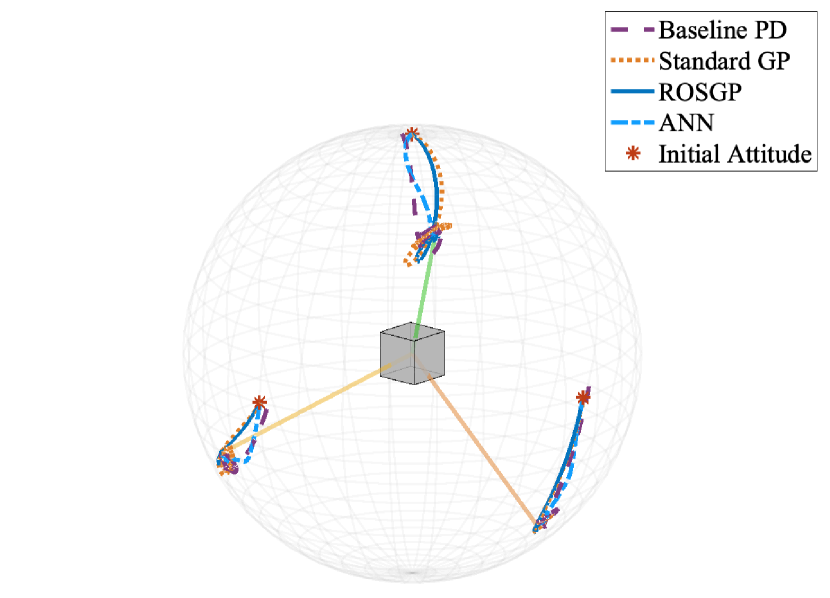
Figure 11: 3-D trajectories of the spacecraft under the considered controllers.

Figure 12: Value of the true uncertain dynamics (given by blue) for each angular acceleration, the mean of the learnt ROSGP (given by red), and the 95% confidence interval (given by shaded blue) evaluated at the true state values at time $t$ when re-maneuvers to the untrained area.

The trajectories of the system states, control inputs, together with the feedback gain under these settings are depicted in Figs. 9-10. It can be seen that under the additional disturbances, both the dynamic response and steady-state error of the baseline PD and standard GP-based schemes are obviously unsatisfactory and fail to sufficiently well perform the attitude re-orientation task, resulting in an oscillating behavior around the equilibrium points. The reason is that the high-gain feedback of the baseline PD controller is not capable of dealing with such large uncertainties anymore, which also cannot be precisely captured by the offline-trained standard GP model. The performance of the proposed ROSGP-based controller is significantly better compared to the baselines, mainly resulting from the online adaptation of the GP compensation strategy. Particularly, compared with ANN method, the system states converge faster under the proposed ROSGP-based controller because of the adaptive feedback gains with GP predictive variance. A 3D illustration of the trajectories of the axes of $\mathcal{F}_{\mathrm{B}}$ is shown in Fig. 11, where the gray cube in the center represents the combined spacecraft. One can observe that the trajectories under the baseline PD controller show an obvious limit cycle behavior around the desired orientation. This phenomenon can be further demonstrated by Fig. 12.

As shown in Fig. 12, the predictive variance (depicted by a shaded area of 95% confidence interval) keeps at a low level from 50s to 150s during the stabilization task. Next, the predictive variance increases significantly from 150s when the combined spacecraft re-maneuvers to an area outside the training data set. This makes it so that the feedback gain of the two GP-based learning controllers appropriately increases to further mitigate the suddenly appearing time-varying disturbance.

Figure 13: Absolute value of the estimation error $e_{\Delta,j}$ for each dimension $j$ under the considered controllers evaluated over time under the re-orientation scenario.

Figure 13 shows the absolute value of the estimation error $e_{\Delta,j}=\|\mu_{\Delta,j}-\breve{\Delta}_{j}\|$ of the two GPs and $e_{\Delta,j}=\|\hat{\Delta}_{j}-\breve{\Delta}_{j}\|$ of the ANN starting from 150s, i.e., the re-maneuver task begins. It can be observed that despite the presence of target attitude maneuvers, external time-varying disturbances, and unlearnt dynamics, the ROSGP still has the capability of online learning of complicated time-varying uncertainties and compensating for them. Therefore, despite realizing an attitude re-orientation in a previously unseen area of the state space, the set point error can always be maintained at a low level with superior transient performance. It should be noted that the ANN method results in a comparable estimation error w.r.t. the proposed ROSGP, but this comes at the cost of a significant manual tuning of the hyperparameters of the ANN scheme.

In addition, the computation time for a 400s long simulation (on a MacOS Monterey, 10-core M1 Pro, 16GB RAM) under different controllers is illustrated as follows. Particularly, the time costs of the standard GP and ROSGP-based controller during model training is $5.59$s and $2.71$s while during task execution of a $400$s long trajectory. The average computation time of the standard GP, ROSGP, and ANN-based controller per control cycle is $16.36$ms, $3.31$ms, and $3.99$ms (which are realizable under the sampling time $T_{\mathrm{s}}=100$ms), respectively. This shows that the computational load of the proposed control strategy is quite small, and does not require extensive parameter tuning procedures. Thus, the results are consistent with the expected performance of the control system design, indicating that the proposed strategy can efficiently, yet accurately learn the unknown function online, and achieve high-precision control of the attitude takeover task.

5.4 Monte Carlo Simulation

Finally, Monte Carlo simulation is conducted to comprehensively analyze the effectiveness and generalization of the proposed control strategy under different physical parameter values and user chosen controller parameters. Table. 2 presents the range of the selected random parameters in the Monte Carlo simulation.

Table 2: Randomized parameter ranges in the Monte Carlo study.

Randomized Parameters	Range
$m_{\mathrm{t}}$, kg	[50,100]
$\bm{J}_{\mathrm{t}}$, kg$\cdot$m2	$\rm{diag}[50\pm 50,~{}50\pm 50,~{}50\pm 50]$
$\bm{Q}_{0}$	${\mathbb{Q}}^{3}$
$\bm{\omega}_{0}$, rad/s	[-0.1,0.1]$\times$[-0.1,0.1]$\times$[-0.1,0.1]
Baseline $\bm{K}_{\mathrm{p}}$	$[0.08,~{}0.25]\bm{J}_{\mathrm{c}0}$
Baseline $\bm{K}_{\mathrm{d}}$	$[0.28,0.55]\bm{J}_{\mathrm{c}0}$
$\bm{P}[0]$	[1, 1000]$\bm{I}_{M}$
$\bm{K}_{\mathrm{pt}}$	$[0.01,0.3]\bm{J}_{\mathrm{t}}$
$\bm{K}_{\mathrm{dt}}$	$[0.02,0.8]\bm{J}_{\mathrm{t}}$
Amplitude of $\bm{\tau}_{\mathrm{d}}(t)$	[-0.5,0.5]$\times$[-0.5,0.5]$\times$[-0.5,0.5]

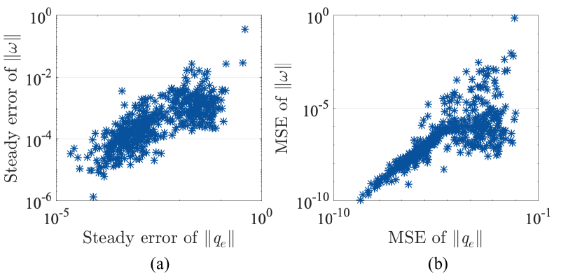
Figure 14: Distributions of (a) steady-state error and (b) MSE of $\bm{q}_{\mathrm{e}}$ and $\bm{\omega}$.

Figure 14 presents the distributions of the steady-state error and mean square error (MSE) of $\bm{q}_{\mathrm{e}}$ and $\bm{\omega}$ from 500 Monte Carlo simulations, respectively, where each “*” represents a simulation case under random conditions. It can be observed that the overwhelming majority of the simulation cases correspond to good performance, where the steady-state error of the attitude quaternion is less than $1\times 10^{-2}$ and that of attitude angular velocity is less than $1\times 10^{-2}\rm{rad/s}$. Additionally, the MSE of attitude quaternion is less than $1\times 10^{-4}$, and that of attitude angular velocity is less than $1\times 10^{-4}\rm{rad/s}$. The results illustrate the generalization performance of the proposed ROSGP-based controller.

In summary, the simulation results show that the proposed GP-based online learning control strategy presented in (41) and Algorithm 1 is highly effective and its implementation is feasible for OOS attitude takeover tasks even in the presence of target attitude maneuverability.

6 CONCLUSION

This paper presents an effective GP-based online learning control strategy for attitude takeover control of noncooperative targets with attitude maneuverability. A novel recursive online sparse GP algorithm is introduced to ensure the successive online learning of the unknown dynamics, while the computational load is kept low, making the approach well applicable in resource-constrained onboard scenarios. The proposed method has probabilistic guarantees for a user-defined bound of the pointing error. The introduced approach provides new perspectives into the attitude controller design of spacecrafts with unknown dynamics, especially in cases where the moment of inertia cannot be identified. The properties and effectiveness of our proposed strategy have been analyzed and demonstrated by numerical simulations based on a high-fidelity simulator.

References

- [1] A. Flores-Abad, O. Ma, K. Pham, and S. Ulrich A review of space robotics technologies for on-orbit servicing Prog. Aerosp. Sci., vol. 68, pp. 1–26, 2014.
- [2] D. Pinard, S. Reynaud, P. Delpy, and S. E. Strandmoe Accurate and autonomous navigation for the ATV Aerosp. Sci. Technol., vol. 11, no. 6, pp. 490–498, 2007.
- [3] H. Liu, Z. Li, Y. Liu, M. Jin, F. Ni, and Y. Liu Key technologies of TianGong-2 robotic hand and its on-orbit experiments Sci. Sin. Technol., vol. 48, no. 12, pp. 1313–1320, 2018.
- [4] E. Bergmann, B. K. Walker, and D. R. Levy Mass property estimation for control of asymmetrical satellites J. Guid., Control, Dyn., vol. 10, no. 5, pp. 483–491, 1987.
- [5] Y. Murotsu, K. Senda, M. Ozaki, and S. Tsujio Parameter identification of unknown object handled by free-flying space robot J. Guid., Control, Dyn., vol. 17, no. 3, pp. 488–494, 1994.
- [6] O. Ma, H. Dang, and K. Pham On-orbit identification of inertia properties of spacecraft using a robotic arm J. Guid., Control, Dyn., vol. 31, no. 6, pp. 1761–1771, 2008.
- [7] O.-O. Christidi-Loumpasefski and E. Papadopoulos On the parameter identification of free-flying space manipulator systems Robot. Auton. Syst., vol. 160, p. 104310, 2023.
- [8] O.-O. Christidi-Loumpasefski, G. Rekleitis, E. Papadopoulos, and F. Ankersen On system identification of space manipulator systems including their fuel sloshing effects IEEE Robot. Autom. Lett., vol. 8, no. 5, pp. 2446–2453, 2023.
- [9] Q. Meng, J. Liang, and O. Ma Identification of all the inertial parameters of a non-cooperative object in orbit Aerosp. Sci. Technol., vol. 91, pp. 571–582, 2019.
- [10] W. Chu, S. Wu, Z. Wu, and Y. Wang Least square based ensemble deep learning for inertia tensor identification of combined spacecraft Aerosp. Sci. Technol., vol. 106, p. 106189, 2020.
- [11] P. Huang, D. Wang, Z. Meng, F. Zhang, and J. Guo Adaptive postcapture backstepping control for tumbling tethered space robot-target combination J. Guid., Control, Dyn., vol. 39, no. 1, pp. 150–156, 2015.
- [12] B. Zhang, B. Liang, Z. Wang, Y. Mi, Y. Zhang, and Z. Chen Coordinated stabilization for space robot after capturing a noncooperative target with large inertia Acta Astronaut, vol. 134, pp. 75–84, 2017.
- [13] G. Kang, J. Wu, C. Jin, and X. Chen Adaptive controller design for satellite attached by non-cooperative object Chin. J. Aeronaut., vol. 33, no. 3, pp. 1006–1015, 2020.
- [14] C. Liu, X. Yue, and Z. Yang Are nonfragile controllers always better than fragile controllers in attitude control performance of post-capture flexible spacecraft? Aerosp. Sci. Technol., vol. 118, p. 107053, 2021.
- [15] H. Leeghim, Y. Choi, and H. Bang Adaptive attitude control of spacecraft using neural networks Acta Astronaut, vol. 64, no. 7, pp. 778–786, 2009.
- [16] P. Huang, D. Wang, Z. Meng, F. Zhang, and Z. Liu Impact dynamic modeling and adaptive target capturing control for tethered space robots with uncertainties IEEE/ASME Trans. Mechatronics, vol. 21, no. 5, pp. 2260–2271, 2016.
- [17] K. Ning, B. Wu, and C. Xu Event-triggered adaptive fuzzy attitude takeover control of spacecraft Adv. Space. Res, vol. 67, no. 6, pp. 1761–1772, 2021.
- [18] C. Wei, J. Luo, H. Dai, and J. Yuan Adaptive model-free constrained control of postcapture flexible spacecraft: a Euler-Lagrange approach J. Vib. Contr., vol. 24, no. 20, pp. 4885–4903, 2018.
- [19] J. Luo, Z. Yin, C. Wei, and J. Yuan Low-complexity prescribed performance control for spacecraft attitude stabilization and tracking Aerosp. Sci. Technol., vol. 74, pp. 173–183, 2018.
- [20] Y. Fan and W. Jing Inertia-free appointed-time prescribed performance tracking control for space manipulator Aerosp. Sci. Technol., p. 106896, 2021.
- [21] C. E. Rasmussen Gaussian processes in machine learning In Advanced Lectures on Machine Learning. Berlin, Germany: Springer, 2004, pp. 63–71.
- [22] T. Beckers, D. Kulić, and S. Hirche Stable Gaussian process based tracking control of Euler–Lagrange systems Automatica, vol. 103, pp. 390–397, 2019.
- [23] Y. Liu and R. Tóth Learning based model predictive control for quadcopters with dual Gaussian process In Proc. IEEE Conf. Decis. Control (CDC). Austin, TX, USA, December 14-17, 2021, pp. 1515–1521.
- [24] J. Kabzan, L. Hewing, A. Liniger, and M. N. Zeilinger Learning-based model predictive control for autonomous racing IEEE Robot. Automat. Lett., vol. 4, no. 4, pp. 3363–3370, 2019.
- [25] L. Csató and M. Opper Sparse on-line Gaussian processes Neural Comput., vol. 14, no. 3, pp. 641–668, 2002.
- [26] R. C. Grande, G. Chowdhary, and J. P. How Experimental validation of bayesian nonparametric adaptive control using Gaussian processes J. Aerosp. Inform. Syst., vol. 11, no. 9, pp. 565–578, 2014.
- [27] G. Chowdhary, H. A. Kingravi, J. P. How, and P. A. Vela Bayesian nonparametric adaptive control using Gaussian processes IEEE Trans. Neural Netw. Learn. Syst., vol. 26, no. 3, pp. 537–550, 2014.
- [28] D. I. Ignatyev, H.-S. Shin, and A. Tsourdos Sparse online Gaussian process adaptation for incremental backstepping flight control Aerosp. Sci. Technol., vol. 136, p. 108157, 2023.
- [29] D. Petelin and J. Kocijan Control system with evolving Gaussian process models In Proc. IEEE Workshop on Evolving and Adaptive Intelligent Systems (EAIS), 2011, pp. 178–184.
- [30] J. Kocijan Modelling and control of dynamic systems using Gaussian process models. Springer, 2016.
- [31] M. Maiworm, D. Limon, and R. Findeisen Online learning-based model predictive control with gaussian process models and stability guarantees Int. J. Robust Nonlinear Control, vol. 31, no. 18, pp. 8785–8812, 2021.
- [32] G. Ma, Y. Liu, Y. Lyu, and P. Wang Learning-based attitude takeover control for noncooperative space targets with unknown dynamics In Proc. IEEE Chin. Control Conf. (CCC). Shanghai, China, July, 2021, pp. 2233–2238.
- [33] B. Wie Space Vehicle Dynamics and Control. Reston, VA, USA: AIAA Education Series, 2008.
- [34] Z. Chen and B. Wang How priors of initial hyperparameters affect Gaussian process regression models Neurocomputing, vol. 275, pp. 1702–1710, 2018.
- [35] R. L. Burden, J. D. Faires, and A. M. Burden Numerical analysis. 10th ed. Boston, MA, USA: Cengage Learning, 2014.
- [36] E. Snelson and Z. Ghahramani Sparse Gaussian processes using pseudo-inputs Adv. Neural Inf. Process. Syst., vol. 18, pp. 1257–1264, 2005.
- [37] J. Umlauft, L. Pöhler, and S. Hirche An uncertainty-based control Lyapunov approach for control-affine systems modeled by Gaussian process IEEE Control Syst. Lett., vol. 2, no. 3, pp. 483–488, 2018.
- [38] N. Srinivas, A. Krause, S. M. Kakade, and M. W. Seeger Information-theoretic regret bounds for Gaussian process optimization in the bandit setting IEEE Trans. Inf. Theory, vol. 58, no. 5, pp. 3250–3265, 2012.
- [39] J. Umlauft and S. Hirche Feedback linearization based on Gaussian processes with event-triggered online learning IEEE Trans. Automat. Control, vol. 65, no. 10, pp. 4154–4169, 2019.
- [40] H. Gui and A. H. de Ruiter Robustness analysis and performance tuning for the quaternion proportional–derivative attitude controller J. Guid., Control, Dyn., vol. 41, no. 10, pp. 2308–2317, 2018.
- [41] P. Huang, M. Wang, Z. Meng, F. Zhang, Z. Liu, and H. Chang Reconfigurable spacecraft attitude takeover control in post-capture of target by space manipulators J. Franklin Inst., vol. 353, no. 9, pp. 1985–2008, 2016.