COPF: Continual Learning Human Preference through Optimal Policy Fitting

Abstract

The technique of Reinforcement Learning from Human Feedback (RLHF) is a commonly employed method to improve pre-trained Language Models (LM), enhancing their ability to conform to human preferences. Nevertheless, the current RLHF-based LMs necessitate full retraining each time novel queries or feedback are introduced, which becomes a challenging task because human preferences can vary between different domains or tasks. Retraining LMs poses practical difficulties in many real-world situations due to the significant time and computational resources required, along with concerns related to data privacy. To address this limitation, we propose a new method called Continual Optimal Policy Fitting (COPF), in which we estimate a series of optimal policies using the Monte Carlo method, and then continually fit the policy sequence with the function regularization. COPF involves a single learning phase and doesn’t necessitate complex reinforcement learning. Importantly, it shares the capability with RLHF to learn from unlabeled data, making it flexible for continual preference learning. Our experimental results show that COPF outperforms strong Continuous learning (CL) baselines when it comes to consistently aligning with human preferences on different tasks and domains.

1 Introduction

In the realm of natural language processing (NLP), large language models (LLMs) are vital tools with the potential to bridge human language and machine understanding. Learning human preferences is a crucial step towards ensuring that language models not only generate responses that are useful to users but also adhere to ethical and societal norms, namely helpful and harmless responses [1]. However, they face a fundamental challenge in aligning with human preferences and values, hindering their full potential. Traditional alignment methods, namely Reinforcement Learning from Human Feedback (RLHF)[2, 3], involve supervised fine-tuning (SFT), reward model (RM) training, and policy model training. This complex pipeline lacks flexibility for continual learning (CL) of human preferences, hence existing work[1] often necessitates retraining models to adapt to dynamic preferences. Hence, there is a pressing need for research into continual alignment methods to address this limitation, enabling LLMs to better adhere to evolving human preferences and values while generating helpful responses.

In this paper, we propose an innovative approach to address these challenges by enhancing the utility of the Deterministic Policy Optimization (DPO)[4] algorithm, a non-reinforcement learning, and a non-continual learning method. DPO, rooted in rigorous reinforcement learning theory, offers promising advantages but suffers from three critical limitations:

1. DPO is not supported for evolving human preferences which is common in real-world applications.

2. Instability during the initial training phase, characterized by a substantial gap between reward estimate 3.1 and the ground-truth reward function.

3. A tendency to over-optimize[5] by increasing positive sample generation probability while decreasing negative sample generation probability, leading to text degeneration[6] responses.

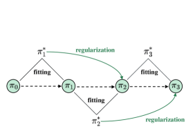
(a) framework

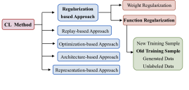
(b) taxonomy

Figure 1: (a) The framework of COPF. The optimal policy $\pi_{t}^{*}$ $(t=1,2,3)$ is derived from the policy $\pi_{t-1}$. The optimal policy $\pi_{t}^{*}$ is utilized as the fitting objective of $\pi_{t}$ and the regularization term of $\pi_{t+1}$. (b) A state-of-the-art and elaborated taxonomy [7] of representative continual learning methods. Bold indicates the category to which our method belongs.

To overcome these limitations, we introduce improvements to DPO’s theoretical optimization objectives. Our approach, as illustrated in Figure 1(a), involves employing Monte Carlo estimation to derive a sequence of optimal policies ($\pi^{*}_{1}\rightarrow\pi^{*}_{2}\rightarrow\pi^{*}_{3}$) in tasks with continuously changing human preferences. This estimation is then incorporated into the probability distribution for positive and negative examples of the optimal policies based on real data. We directly fit this probability distribution, and retain a small amount of old task data while recording their distributions under the optimal policy. Meanwhile, when learning new tasks, we employ a function regularization[7] strategy to maintain performance on previous tasks.

To the best of our knowledge, we are the first to study the CL of alignment methods. For fair evaluation, we construct the first benchmark for continuous learning of human preferences based on different human preference data (Section 4.3), including Helpful and Harmless preference (HH)[1] data, Standard Human Preference (SHP)[8] data, Reddit TL;DR summary[2] human preference data provided by CarperAI , and the enhanced IMDB[9] Sentiment Text Generation benchmark released by RL4LMs [10].

In summary, our work presents a novel approach, termed "COPF" which leverages improvements to DPO’s theoretical foundations. By doing so, we tackle the challenges associated with learning human preferences in a continual learning scenario, ultimately achieving SOTA performance.

2 Preliminaries

2.1 Static Alignment

Reinforcement Learning from Human Feedback. The recent RLHF pipeline consists of three phases: 1) supervised fine-tuning (SFT); 2) preference sampling and reward learning and 3) reinforcement-learning optimization. In the SFT phases, the language model is fine-tuned with supervised learning (maximum likelihood) on the downstream tasks. In the reward learning phase, human annotators rank multiple answers {$y_{1}$, $y_{2}$, …, $y_{n}$} for a prompt x based on human preferences, generating human feedback data. Then, this feedback data is used to train a reward model, which assigns higher scores to pairs consisting of prompts and answers that are preferred by humans. In the RL Fine-Tuning phase, the mainstream methods maximize a KL-constrained reward objective like

$$\max_{\pi_{\theta}}\mathbb{E}_{x\sim\mathcal{D},y\sim\pi_{\theta}(y\mid x)}\bigl{[}r_{\phi}(x,y)\bigr{]}-\beta\mathbb{D}_{\textrm{KL}}\bigl{[}\pi_{\theta}(y\mid x)\mid\mid\pi_{ref}(y\mid x)\bigr{]}$$ (1)

where $\beta$ is a parameter controlling the deviation from the base reference policy $\pi_{ref}$, namely the initial SFT model $\pi_{sft}$. Because language generation operates discretely, this objective lacks differentiability and is generally optimized using reinforcement learning techniques. The recent approaches [1, 3, 2] reconstruct the reward function ${r(x,y)=r_{\phi}(x,y)-\beta(\log\pi_{\theta}(y\mid x)-\log\pi_{ref}(y\mid x))}$, and maximize using PPO [11].

Direct Preference Optimization. Previous work DPO[4] proposes a direct optimization objective, which requires no reward learning and reinforcement-learning optimization. The objective of DPO is based on the optimal solution to the KL-constrained reward maximization objective:

$$\pi_{r}(y\mid x)=\frac{1}{Z(x)}\pi_{ref}(y\mid x)\exp\left(\frac{1}{\beta}r(x,y)\right)$$ (2)

where $Z(x)=\sum_{y}\pi_{ref}(y\mid x)\exp\left(\frac{1}{\beta}r(x,y)\right)$ is the partition function. In the RLHF scenario, x represents the prompt, and y represents a potential response. Specifically, we first take the logarithm of both sides of Eq.2 and then with some algebra we obtain:

$$r(x,y)=\beta\log\frac{\pi_{r}(y\mid x)}{\pi_{ref}(y\mid x)}+\beta\log Z(x).$$ (3)

When collecting human feedback data, it is common to generate two or multiple answers for a single prompt (which can come from different models or even humans) and then rank the answers based on human preferences. Based on the Eq. 2 and the Bradley-Terry (BT) model, DPO proposes a direct policy objective:

$$\mathcal{L}_{\text{DPO}}(\pi_{\theta};\pi_{ref})=-\mathbb{E}_{(x,y_{w},y_{l})\sim\mathcal{D}}\left[\log\sigma\left(\beta\log\frac{\pi_{\theta}(y_{w}\mid x)}{\pi_{ref}(y_{w}\mid x)}-\beta\log\frac{\pi_{\theta}(y_{l}\mid x)}{\pi_{ref}(y_{l}\mid x)}\right)\right]$$ (4)

2.2 Continual Alignment

In the static alignment, the dataset typically consists of a fixed, static set of examples that are collected and labeled for a specific task. The dataset remains constant throughout the training process. In the continual alignment scenario, the human preference dataset evolves over time, often consisting of a sequence of tasks or domains. Each task or domain may have its own set of data, and these tasks are presented to the model sequentially. The order in which tasks are presented can vary, and the model needs to adapt to new tasks without forgetting previously learned ones.

In this paper, we consider that there is a sequence of tasks $\mathbb{T}=\{\mathcal{T}_{1},\mathcal{T}_{2},...\}$ to learn, and a sequence of corresponding human preference datasets $\mathbb{D}=\{\mathcal{D}_{1},\mathcal{D}_{2},...\}$. The initial policy is the SFT model, namely, $\pi_{0}=\pi_{SFT}$. For each task $\mathcal{T}_{t}(t=1,2,...)$, the policy $\pi_{t}$ is initialized by $\pi_{t-1}$ and there is a latent scoring function (i.e. the reward model) $r_{t}(x,y)$ can be learned from $\mathcal{D}_{t}$. A naive $r_{t}(x,y)$ is that $r_{t}(x,y_{w})=1$ and $r_{t}(x,y_{l})=0$. To mitigate forgetting, we maintain a replay memory buffer $\mathbb{R}=\{\mathcal{R}_{1},\mathcal{R}_{2},...\}$, where $\mathcal{R}_{i}\subset\mathcal{D}_{i}$ ($i=1,2,...,t$) stores training data from 1% of historical tasks. When learning new tasks, the data in the replay memory is merged with the training data of the new task.

3 Method

3.1 Motivation of the Method

The DPO method derives the maximum likelihood optimization solution from the theory of reinforcement learning, and its theoretical foundation is rigorous. However, the optimization process of DPO has two flaws.

• Suboptimal learning results: The gradient of the loss function $\mathcal{L}_{\text{DPO}}$ with respect to the parameters $\theta$ can be written as:

  $$\nabla_{\theta}\mathcal{L}_{\text{DPO}}(\pi_{\theta};\pi_{ref})=\\ -\beta\mathbb{E}_{(x,y_{w},y_{l})\sim\mathcal{D}}\bigg{[}\underbrace{\sigma(\hat{r}_{\theta}(x,y_{l})-\hat{r}_{\theta}(x,y_{w}))}_{\text{higher weight when reward estimate is wrong}}\bigg{[}\underbrace{\nabla_{\theta}\log\pi(y_{w}\mid x)}_{\text{increase likelihood of $y_{w}$}}-\underbrace{\nabla_{\theta}\log\pi(y_{l}\mid x)}_{\text{decrease likelihood of $y_{l}$}}\bigg{]}\bigg{]},$$

  where $\hat{r}_{\theta}(x,y)=\beta\log\frac{\pi_{\theta}(y\mid x)}{\pi_{ref}(y\mid x)}$ is the reward implicitly defined by the language model $\pi_{\theta}$ and reference model $\pi_{ref}$ . In the DPO paper, the author claims that the weight term $\sigma(\hat{r}_{\theta}(x,y_{l})-\hat{r}_{\theta}(x,y_{w}))$ represents how much higher the implicit reward model rates the dispreferred completions. Compared $\hat{r}_{\theta}(x,y)$ with the $r(x,y)$ in Eq 3 , the term $\pi_{\theta}(y\mid x)$ has a significant gap from the $\pi_{r}(y\mid x)$ in the true reward function at the beginning of optimization. Hence, the implicit reward model still has a gap with the true reward model in the learning process, which may lead to suboptimal learning results.

• The risk of over-optimization: In the learning process of DPO, the $\log\pi_{\theta}(y_{w}|x)$ is increased, and the $\log\pi_{\theta}(y_{l}|x)$ is declined. Hence, the weight term $\sigma(\hat{r}_{\theta}(x,y_{l})-\hat{r}_{\theta}(x,y_{w}))=\sigma(\beta\log\pi_{\theta}(y_{w}|x)-\beta\log\pi_{\theta}(y_{l}|x)+\beta\log\pi_{ref}(y_{l}|x)-\beta\log\pi_{ref}(y_{w}|x))$ is also increasing, which exacerbates the widening gap between $\log\pi_{\theta}(y_{w}|x)$ and $\log\pi_{\theta}(y_{l}|x)$ and leads to over-optimization[5] and text degeneration[6]. Although it is possible to control the increase in the gap by the max-margin strategy[12], it introduces a new hyper-parameter to determine the maximal margin.

3.2 Continual Optimal Policy Fitting

Previous works[4, 13], prove that the optimal solution to the KL-constrained reward maximization objective takes the form of Eq. 2. Based on this, we conclude that the optimal policy of task $\mathcal{T}_{t}$ is

$$\pi^{*}_{t}(y|x)=\frac{1}{Z_{t}(x)}\pi_{t-1}(y|x)exp(\frac{1}{\beta}r_{t}(x,y))$$ (5)

where $Z_{t}(x)=\Sigma_{y}\pi_{t-1}(y|x)exp(\frac{1}{\beta}r_{t}(x,y))$ is the partition function, $x\in\mathcal{D}_{t}$ denotes the prompt, $y\in$ denotes the possible response. For the estimation $\pi^{*}_{t}(y|x)$, we suppose that there are $J_{x}$ responses of each prompt $x$ and the partial order annotated by humans is $y_{1}^{x}\prec y_{2}^{x}\prec...\prec y_{J_{x}}^{x}$.

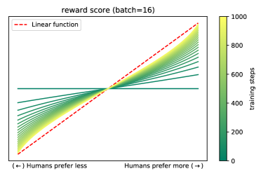
Figure 2: The score distribution of pairwise reward learning.

Step-1: Construct reward function

We introduce 2 methods to determine reward function.

Linear reward: We simulate training the reward model using a pairwise loss function $\mathcal{L}_{ranking}=-\log(\sigma(r_{\theta}(x,y_{w})-r_{\theta}(x,y_{l})))$, where $y_{w}$ and $y_{l}$ represent the human choose and human rejected response respectivey. We found that the reward scores are approximately linearly related to human preferences. We provide theoretical derivations in the Appendix Section A.1. Previous works [14, 15, 16, 17] present the reward as a linear combination of pre-trained features or hand-crafted features. Recent work[18] gets enhanced performance by modeling a linear reward function according to regret which is the negated sum of an optimal policy’s advantage in the segment. Inspired by this, we propose a linear reward according to human preference

$$r_{t}(x,y_{j}^{x})=Adv(x,y_{j}^{x})+\delta(x)$$ (6)

for approximating the well trained reward function, where $j=1,2,...,{J_{x}}$ represents the degree of human preference, the function $\delta(x)$ depends solely on the prompt $x$, $Adv(x,y_{j}^{x})\triangleq\frac{2j-J_{x}-1}{J_{x}}\in(-1,1)$ denotes the advantage score. For a given prompt $x$, if the question is easy to answer, the average reward score should be positive ($\delta(x)>0$), if the question is hard then the average reward score should be negative ($\delta(x)<0$).

Gaussian reward: The Gaussian distribution is also observed in well-trained reward scores[19]. Inspired by this observation, we attempt to modeling the advantage score, i.e., the extra reward one response can obtain compared with the expected reward, by a normal distribution and regulating the advantage score distribution dynamically during training, ensuring that the variances and means are maintained within a reasonable range.

We split the reward $r(x,y)$ into the advantage score $Adv(x,y)$ and the expected reward $E_{y\sim\pi({\cdot|x})}r(x,y)$, where $Adv(x,y)\sim N(0,\sigma)$, $\sigma$ is hyperparameter. Given a prompt $x$, and partially-ordered set of responses $\mathcal{Y}^{x}=\{y_{1}^{x}\prec y_{2}^{x}\prec...\prec y_{J_{x}}^{x}\}$. We sample $J_{x}$ values $\{R_{1}<R_{2}<...<R_{J_{x}}\}$ from the distribution $N(0,\sigma)$, and define $Adv(x,y_{j}^{x})\triangleq{R_{j}}$. Overall, the reward function can be writen as

$$r_{t}(x,y_{j}^{x})=Adv(x,y_{j}^{x})+\delta(x)$$ (7)

for approximating the well trained reward function, where $j=1,2,...,{J_{x}}$ represents the degree of human preference, the expectation $\delta(x)=E_{y\sim\pi({\cdot|x})}r(x,y)$ depends solely on the prompt $x$. In Step-2, we theoretically prove that there is no need to calculate specific values for $\delta(x)$ and partition function $Z(x)$.

Step-2: Calculate the distribution of sampling space $P^{*}_{y\in\mathcal{Y}^{x},t}(y|x)$.

We sample $y$ multiple times to obtain the partially-ordered set $\mathcal{Y}^{x}=\{y_{1}^{x}\prec y_{2}^{x}\prec...\prec y_{J_{x}}^{x}\}$. Due to $\pi^{*}_{t}(y|x)$ is based on the partition function $Z_{t}(x)$ which is hard to estimate. We calculate the re-normalized distribution $P^{*}_{y\in\mathcal{Y}^{x},t}(y|x)$: KL loss task $\mathcal{T}_{t}$:

$$P^{*}_{y\in\mathcal{Y}^{x},t}(y|x) \triangleq\frac{\pi^{*}_{t}(y|x)}{\Sigma_{y^{{}^{\prime}}\in\mathcal{Y}^{x}}\pi^{*}_{t}(y^{{}^{\prime}}|x)}$$ (8)

$$=\frac{\cancel{\frac{1}{Z_{t}(x)}}\cdot\pi_{t-1}(y|x)\cdot exp(\frac{1}{\beta}Adv(x,y))\cdot\cancel{exp(\frac{1}{\beta}\delta(x))}}{\Sigma_{y^{{}^{\prime}}\in\mathcal{Y}^{x}}\cancel{\frac{1}{Z_{t}(x)}}\cdot\pi_{t-1}(y^{{}^{\prime}}|x)\cdot exp(\frac{1}{\beta}Adv(x,y^{{}^{\prime}}))\cdot\cancel{exp(\frac{1}{\beta}\delta(x))}}$$

$$=\frac{\pi_{t-1}(y|x)exp(\frac{1}{\beta}Adv(x,y))}{\Sigma_{y^{{}^{\prime}}\in\mathcal{Y}^{x}}\pi_{t-1}(y^{{}^{\prime}}|x)exp(\frac{1}{\beta}Adv(x,y^{{}^{\prime}}))}$$

Step-3: Fit the distribution $P^{*}_{y\in\mathcal{Y}^{x},t}(y|x)$.

Next, we directly fit the re-normalized probability $P^{*}_{y\in\mathcal{Y}^{x},t}(y|x)$ by minimizing the KL loss task $\mathcal{T}_{t}$:

$$L_{t}^{fit}({\theta}_{t}) =\mathbb{E}_{x\sim{\mathcal{D}_{t}}}\Sigma_{y\in\mathcal{Y}^{x}}D_{KL}(P_{y\in\mathcal{Y}^{x},t}(y|x,{\theta}_{t}),P^{*}_{y\in\mathcal{Y}^{x},t}(y|x))$$ (9)

where $\theta_{t}$ denotes the parameters of the policy model $\pi_{t}(y|x)$ at task $\mathcal{T}_{t}$ $(t=1,2,...)$, and $P_{y\in\mathcal{Y}^{x},t}(y|x,{\theta})$ denotes the re-normalized probability of current model:

$$P_{y\in\mathcal{Y}^{x},t}(y|x,{\theta}_{t})\triangleq\frac{\pi_{t}(y|x)}{\Sigma_{y^{{}^{\prime}}\in\mathcal{Y}^{x}}\pi_{t}(y^{{}^{\prime}}|x)}$$ (10)

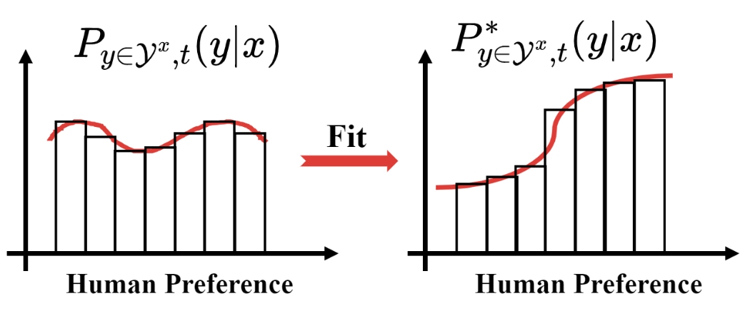
Figure 3: Fitting of $P^{*}_{y\in\mathcal{Y}^{x},t}(y|x)$

Steps 2-3 can be implemeted by 4 lines of codes under the pytorch environment:

⬇

scale_opt = (1 / beta * rm_score.detach()).exp()

P_optimal = P_ref * scale_opt / (P_ref * scale_opt).sum()

P_policy = P_current / P_current.sum()

RDPO_loss = F.kl_div(P_policy.log(), P_optimal)

Step-4: Function Regularization of $\pi_{t}$.

To preserve the old knowledge, we calculate a regularization loss to ensure that the new and old optimal policies do not differ too significantly in terms of the distribution of old human preferences. In detail, for each replay sample $x\in{\mathcal{R}_{i}}$ $(i=1,2,...,t-1)$ , the new policy $\pi_{t}$ is regularized to not differ significantly from the optimzal policy $\pi_{i}^{*}$. Hence, the regularization loss is

$$L_{t}^{reg}({\theta}_{t})=\mathbb{E}_{x\sim{\cup_{i=1}^{i=t-1}\mathcal{R}_{i}}}\Sigma_{i=1}^{t-1}\boldsymbol{I_{\mathcal{R}_{i}}}(x)\cdot\Sigma_{y\in\mathcal{Y}^{x}}D_{KL}(P_{y\in\mathcal{Y}^{x},t}(y|x,{\theta}_{t}),P^{*}_{y\in\mathcal{Y}^{x},i}(y|x))$$ (11)

where $\{\boldsymbol{I_{\mathcal{R}_{i}}}(x)\}_{i=1}^{i=t-1}$ is the set of indicator functions, namely, the task identifier. The final training loss of task $\mathcal{T}_{t}$ is:

$$L_{t}^{train}({\theta}_{t})=\left\{\begin{array}[]{lr}L_{t}^{fit}({\theta}_{t})&x\in{\mathcal{D}_{t}}\\ L_{t}^{reg}({\theta}_{t})&x\in{\cup_{i=1}^{i=t-1}\mathcal{R}_{i}}\end{array}\right.$$ (12)

3.3 Continual Learning on Unlabeled Data

In the above steps of COPF, we learn a policy based on the human preference dataset, where the reward score is determined based on the preference order annotated by humans. We name this mode the hard reward score mode. Inspired by the learned reward model in the RLHF pipeline, we introduce the reward value head, named the linear reward score mode, to learn the human preference scoring on the labeled data at the meanwhile optimal policy fitting process. We find that the reward model head does not need to learn an independent model, like the RLHF pipeline.

In detail, we introduce a value head $\mathcal{V}$ and utilize the pairwise ranking loss $\mathcal{L}_{ranking}$ to learn an RM score, where $\mathcal{L}_{ranking}=-\log(\sigma(r_{\theta}(x,y_{w})-r_{\theta}(x,y_{l})))$, where $y_{w}$ and $y_{l}$ represent the human choose and human rejected response respectively. The final training loss is the sum of $L_{t}^{train}({\theta}_{t})$ and $\mathcal{L}_{ranking}$. After learning the labeled data, the reward value head can be used to score the unlabeled data, and ranking unlabeled responses. (Section 4.5). Based on this ranking, we can utilize the hard mode of the COPF method.

3.4 Comparison with other methods

We compare COPF with current alignment methods in table 1.

Table 1: Compare COPF with other alignment methods.

Method	RL or Non-RL	Online or Offline	Pairwise or Listwise	Token-wise or Trajectory-wise	Invariance [20]	Reward Model	Reference Model	Critic Model	Num of Models	Continual Learning
PPO[11]	RL	online	pairwise	token-wise	no	yes	yes	yes	4	no
NLPO[10]	RL	online	pairwise	token-wise	no	yes	yes	yes	4	no
P3O[20]	RL	online	pairwise	trajectory-wise	yes	yes	yes	no	3	no
PRO[21]	non-RL	offline	listwise	trajectory-wise	-	no	no	no	1	no
DPO[4]	non-RL	offline	pairwise	trajectory-wise	-	no	yes	no	2	no
RAFT[22]	non-RL	both	listwise	trajectory-wise	yes	yes	no	no	2	no
RRHF[23]	non-RL	offline	listwise	trajectory-wise	yes	yes	no	no	2	no
CoH[24]	non-RL	offline	pairwise	trajectory-wise	-	no	no	no	1	no
COPF	non-RL	both	listwise	trajectory-wise	-	no	yes	no	2	yes

Comparison with DPO:

1. DPO uses the log ratio as a reward value, while COPF uses a custom reward (linear or gaussian).

2. DPO employs pairwise training, while COPF uses listwise training.

3. DPO maximizes the gap between wins and losses, while COPF fits the distribution of the optimal policy on the sampled dataset.

Comparison with PRO:

1. PRO enhances the probability of top-ranked samples occupying all sampled instances, while COPF fits the optimal policy distribution.

2. PRO is optimized based on intuitive reasoning and does not use a reference model, while COPF is derived from reinforcement learning theory as an optimization objective and requires the use of a reference model.

4 Experiments

4.1 Datasets

Stanford Human Preferences (SHP) Dataset[8]: SHP is a dataset of 385K collective human preferences over responses to questions/instructions in 18 different subject areas, from cooking to legal advice. The preferences are meant to reflect the helpfulness of one response over another and are intended to be used for training RLHF reward models and NLG evaluation models (e.g., SteamSHP).

Helpful and Harmless (HH) [1]: The HH-RLHF dataset is collected by two separate datasets using slightly different versions of the user interface. The helpfulness dataset is collected by asking crowdworkers to have open-ended conversations with models, asking for help, and advice, or for the model to accomplish a task, and to choose the more helpful model response. The harmlessness or red-teaming dataset is collected by asking crowd workers to attempt to elicit harmful responses from our models and to choose the more harmful response offered by the models.

Reddit TL;DR: For each Reddit post in the Reddit TL;DR [25] dataset, multiple summaries are generated using various models. These models include pre-trained ones used as zero-shot summary generators, as well as supervised fine-tuned models (12B, 6B, and 1.3B) specifically trained on the Reddit TL;DR dataset. Additionally, the human-written TL;DR (reference) is considered as a sample for comparison.

IMDB: We consider the IMDB dataset for the task of generating text with positive sentiment. The IMDB text continuation task aims to positively complete the movie review when given a partial review as a prompt. In this task, a trained sentiment classifier DistilBERT[26] is provided as a reward function to train the RL agents and evaluate their task performance. The naturalness of the trained model is evaluated with a perplexity score. The dataset consists of 25k training, 5k validation, and 5k test examples of movie review text with sentiment labels of positive and negative. The input to the model is a partial movie review text (up to 64 tokens) that needs to be completed (generating 48 tokens) by the model with a positive sentiment while retaining fluency. For RL methods, we use a sentiment classifier that is trained on pairs of text and labels as a reward model which provides sentiment scores indicating how positive a given piece of text is.

4.2 Baselines

Supervise fine-tuning (SFT) directly learns the human-labeled summary through the cross-entropy loss. We combine SFT with classic continual learning methods.

• SFT-Online L2Reg penalizes the updating of model parameters through an L2 loss $L_{2}^{t}(\theta)=\sum_{i}({\theta}^{i}_{t}-{\theta}^{i}_{t-1})^{2}$. This regularization term mitigates the forgetting issue by applying a penalty for every parameter change.

• SFT-EWC [27] uses fisher information to measure the parameter importance to old tasks, then slows down the update of the important parameters by L2 regularization.

• SFT-MAS [28] computes the importance of the parameters of a neural network in an unsupervised and online manner to restrict the updating of parameters in the next task.

• SFT-AGM [29] is an improved version of GEM [30], which enjoys better performance than GEM, while being almost as computationally and memory efficient as EWC and other regularization based methods.

• SFT-LwF [31] is a knowledge-distillation-based method, which computes a smoothed version of the current responses for the new examples at the beginning of each task, minimizing their drift during training.

• SFT-TFCL [32] proposes to timely update the importance weights of the parameter regularization by detecting plateaus in the loss surface.

• SFT-DER++[33] addresses the General Continual Learning (GCL) problem by mixing rehearsal with knowledge distillation and regularization, in which the logits and ground truth labels of part of old data are saved into the memory buffer for replaying.

Recent alignment methods are not support for continual, we improve those methods with continual tricks.

Ranking-based Approachs[4, 21, 20, 23, 22] rank human preferences over a set of responses and directly incorporate the ranking information into the LLMs fine-tuning stage.

• DPO^C[4] is an offline approach that can directly align LM with human preference data, drawing from the closed-form solution of the Contextual Bandit with KL control problem.

• PRO^C[21] learns preference ranking data by initiating with the first prefered response, deems subsequent responses as negatives, then dismisses the current response in favor of the next.

• RRHF^C[23] aligns with human preference by a list rank loss and finds that the SFT training objective is more effective and efficient than KL-divergence in preventing LLMs from over-fitting

Language-based Approach directly use natural language to inject human preference via SFT.

• CoH^C[24] directly incorporates human preference as a pair of parallel responses discriminated as low-quality or high-quality using natural language prefixes. CoH only applies the fine-tuning loss to the actual model outputs, rather than the human feedback sequence and the instructions. During inference, CoH directly puts position feedback (e.g.,good) after the input instructions to encourage the LLMs to produce high-quality outputs.

4.3 Tasks and Evaluation Metrics

Table 2: Various tasks, input and output types, and the metrics used in the TIL settings.

Dataset	Task	Input	Output	Preference Metric	Naturalness Metric(s)
IMDB[9]	Text Continuation	Partial Movie Review	A positive completion of the movie review.	70M sentiment classifier DistilBERT	RougeL, BLEU-4, METEOR
HH-RLHF[1]	Helpful & Harmless Question Answering	Question	A helpful and harmless answer to the question	2.7B SteamSHP- flan-t5-xl model
Reddit TL;DR[2]	Summarization	Reddit POST	Summarized POST	6.7B GPT-J reward model by Carper-AI

Task Incremental Learning (TIL) setting: The policy is required with continuous learning across three distinct tasks: the QA task on the HH-RLHF dataset, the summary task on the Reddit TL;DR dataset, and the positive file review generation task on the IMDB dataset.

Evaluation metrics for TIL: As shown in Table 2, we utilize 3 preference metrics and 3 naturalness metrics to evaluate the performance of the model. In detail, we employ the SteamSHP-flan-t5-xl model [8], developed by Stanford, as the preference model (PM) for assessing responses to HH-RLHF prompts. Additionally, we utilize the 6.7B gpt-j reward model , released by Carper-AI, to evaluate summaries of Reddit posts. Furthermore, we gauge the positivity of generated film reviews by assessing them using the distilbert-imdb model [26].

Domain Incremental Learning (DIL) setting: The policy is required to continuously learn from three segments of the SHP dataset. The SHP dataset comprises 18 domains, which we have divided into three parts. To elaborate, we have trained 18 preference models (PM), each corresponding to one of the 18 domains. Subsequently, we assess the performance of each PM across all 18 domains. We record the performance decline observed when a PM trained on one domain is evaluated on the others. Finally, we partition the 18 domains into three groups based on the highest observed performance decline. Further details can be found in the Appendix Section B.

Evaluation metrics for DIL: We employ the SteamSHP-flan-t5-xl model [8], developed by Stanford, as the preference model (PM) for assessing responses to SHP prompts. The SteamSHP-flan-t5-xl model is trained on the combination of the SHP (all 18 domains) and the HH-RLHF human preference data.

Evaluation Metric for Continual Learning

Overall performance is typically evaluated by average accuracy (AA)[34, 30] and average incremental accuracy (AIA) [35, 36]. In our evaluation setting, the accuaracy is replaced by the Preference Metric (0-1). Let ${a}_{k,j}\in[0,1]$ denote the Preference Score evaluated on the test set of the $j$-th task after incremental learning of the $k$-th task ($j\leq k$). The two metrics at the $k$-th task are then defined as

$${{\rm{AA}}_{k}}=\frac{1}{k}\sum_{j=1}^{k}{a}_{k,j},$$ (13)

$${{\rm{AIA}}_{k}}=\frac{1}{k}\sum_{i=1}^{k}{\rm{AA}}_{i},$$ (14)

where AA represents the overall performance at the current moment and AIA further reflects the historical variation.

Memory stability can be evaluated by forgetting measure (FM) [34] and backward transfer (BWT) [30]. As for the former, the forgetting of a task is calculated by the difference between its maximum performance obtained in the past and its current performance:

$$f_{j,k}=\max_{i\in\{1,...,k-1\}}({a}_{i,j}-{a}_{k,j}),\forall j<k.$$ (15)

FM at the $k$-th task is the average forgetting of all old tasks:

$${{\rm{FM}}_{k}}=\frac{1}{k-1}\sum_{j=1}^{k-1}f_{j,k}.$$ (16)

As for the latter, BWT evaluates the average influence of learning the $k$-th task on all old tasks:

$${\rm{BWT}}_{k}=\frac{1}{k-1}\sum_{j=1}^{k-1}({a}_{k,j}-{a}_{j,j}),$$ (17)

where the forgetting is usually reflected as a negative BWT.

4.4 Results of Continual Learning from Human Preferences

Table 3 shows the test results of continual learning from human preferences on the TIL setting. Figure 4 shows the valid results of continual learning from human preferences on TIL setting.

Table 3: The performances at last task in the TIL scenario. Italic indicates methods based on Supervised Fine-Tuning that did not use pair data and only utilized prompt and chosen data. For fair comparison, all baselines utilize 1% historical replay data. COPF^L and COPF^G denote the linear and gaussian reward respectively. Due to the original CoH, DPO and PRO methods are not supported for continual learning, we introduce the CoH^C, DPO^C and PRO^C by adding the Function Regularization loss for continual learning. All of experiments are based on the Llama-7b PLM.

Method / Taxonomy	HH-RLHF	Reddit TL:DR	IMDB	Overall performance		Memory stability
	SteamSHP (↑)	Gpt-J (↑)	DistillBert (↑)	AA (↑)	AIA (↑)	BWT (↑)	FM (↓)
L2-Reg / function regularization	0.797	0.812	0.812	0.807	0.807	-0.028	0.031
EWC[27] / weight regularization	0.803	0.821	0.826	0.817	0.821	-0.026	0.026
MAS[28] / weight regularization	0.807	0.819	0.812	0.813	0.819	-0.027	0.027
AGM[29] / gradient projection	0.812	0.827	0.832	0.824	0.829	-0.022	0.024
LwF[31] / function regularization	0.813	0.841	0.833	0.829	0.820	-0.024	0.024
TFCL[32] / weight regularization	0.813	0.832	0.829	0.825	0.821	-0.021	0.021
DER++[33] / experience replay	0.815	0.837	0.841	0.831	0.836	-0.017	0.019
CoHC[24] / experience replay	0.807	0.883	0.825	0.838	0.854	-0.027	0.027
PROC[21] / experience replay	0.795	0.876	0.854	0.842	0.857	-0.038	0.038
RRHFC[23] / experience replay	0.807	0.867	0.861	0.845	0.848	-0.020	0.020
DPOC[4] / function regularization	0.825	0.875	0.844	0.848	0.862	-0.026	0.026
COPFL / function regularization	0.836	0.877	0.876	0.863	0.851	0.006	-0.006
COPFG / function regularization	0.856	0.895	0.815	0.855	0.878	-0.021	0.021

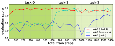
(a) COPF replay ratio : 0.01

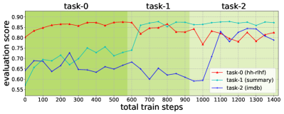
(b) DPO replay ratio : 0.01

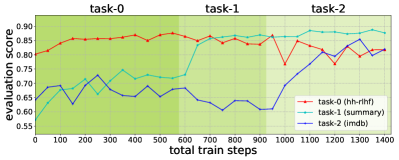
(c) PRO replay ratio : 0.01

(d) RRHF replay ratio : 0.01

Figure 4: Evaluation curves of TIL setting.

4.5 Can COPF make effective use of unlabeled prompts?

In this section, we discuss how the COPF policy makes use of unlabeled prompts. Standard RLHF methods can leverage additional unlabeled prompts by labeling LM generations with the learned reward model. Inspired by the learned reward model, we introduce the reward value head, namely the linear reward score mode, to learn the human preference scoring on the labeled data at the meanwhile of optimal policy fitting process. We find that the two objectives are not in conflict.

Table 4: Performance on DIL setting in which part of data is unlabeled.

	Domains 1-6	Domains 7-12	Domains 13-18	Overall performance		Memory stability
Method	SteamSHP (↑)	SteamSHP (↑)	SteamSHP (↑)	AA (↑)	AIA (↑)	BWT (↑)	FM (↓)
COPFL / label	0.881	0.901	0.909	0.897	0.873	0.027	-0.015
COPFL / task-2 unlabel	0.881	0.912	0.913	0.902	0.874	0.033	-0.020
COPFL / task-1,2 unlabel	0.873	0.883	0.904	0.887	0.870	0.015	0.000

After learning about the labeled data, we utilize the LM with the value head as explicit RM. We suppose that for each prompt $x$, there are multiple responses $\mathbf{{Y}}^{x}=\{y_{1}^{x},y_{2}^{x},...,y_{J_{x}}^{x}\}$ without knowing the human preference order. The responses can be generated by the trained policy or collected by other models or humans, like the PPO method. Then we utilize the explicit reward model to sort responses in set $\mathbf{{Y}}^{x}$. We conduct an experiment on the SHP dataset under the DIL setting. The LM is trained in the first 6 domains to learn the ability to score and to align with human preference. Then the LM with a value head is treated as an explicit RM to score the the unlabeled pairwise data. Here, we utilize the same prompts and responses in the SHP data, but the preference order is sorted by the explicit RM.

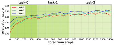
(a) DIL on labeled data

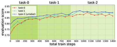
(b) DIL on ublabeled task-2

Figure 5: Evaluation curves of DIL setting.

Figure 5 shows the results of continual learning from human preferences on DIL setting. In Table 4, we compare the learning results on unlabeled prompts and on the original SHP data. An observation from the learning results is that learning on unlabeled task-2 has better performance than learning on all labeled tasks.

5 Related Work

5.1 Taxonomy of representative continual learning methods

As illustrated in Figure 1(b), within the realm of continual learning, several noteworthy methodologies emerge, encompassing the regularization-based approach, replay-based techniques, optimization-based strategies, representation-based methodologies, and architecture-based innovations [7].

The Regularization-Based Approach orchestrates the introduction of explicit regularization terms, thereby striving to strike a harmonious balance between the acquisition of new skills and the retention of past knowledge. Weight regularization [27, 28, 34]is concerned with tempering the fluctuation of network parameters, often achieved by integrating a quadratic penalty term into the loss function. In contrast, function regularization[31, 37] turns its focus to the intermediate or final output of the prediction function.

The Replay-Based Approach presents a multifaceted strategy encompassing three distinct sub-directions. The initial approach, experience replay[38], revolves around the retention of a limited cache of prior training samples within a compact memory buffer. The second approach, generative replay or pseudo-rehearsal [39], entails the training of an additional generative model tasked with reproducing synthetic data samples. In contrast, feature replay[40] diverges from its counterparts by maintaining feature-level distributions, bypassing the replication of entire data samples.

The Optimization-Based Approach navigates the terrain of continual learning through explicit design and manipulation of optimization programs. This includes techniques such as gradient projection[30], and meta-learning[41]. Gradient projection serves as a mechanism for constraining parameter updates, ensuring alignment with the trajectory of experience replay. Meta-learning, often referred to as "learning-to-learn" within the context of continual learning, endeavors to cultivate a data-driven inductive bias adaptable to various scenarios, thus eliminating the need for manual design.

The Representation-Based Approach leverages the strengths of self-supervised learning (SSL)[42] and large-scale pre-training[43] to enhance the quality of representations at both the initialization and continual learning stages. This category encompasses self-supervised learning (primarily employing contrastive loss) for continual learning, pre-training for downstream continual learning, and continual pre-training (CPT)[44] or continual meta-training[45].

The Architecture-Based Approach addresses inter-task interference by fashioning task-specific parameters. This approach can be dissected into three distinct paradigms: parameter allocation[46], where dedicated parameter subspaces are allocated to each task, either maintaining a fixed or dynamic network architecture; model decomposition[47], which explicitly segregates a model into task-sharing and task-specific components, with the latter typically being expandable; and modular networks[48], which harness parallel sub-networks or sub-modules to facilitate differentiated learning of incremental tasks, devoid of pre-defined task-sharing or task-specific components.

5.2 Learning from Human Preferences

Learning from human preferences has been studied in the game field [49, 50, 51, 52] and has recently been introduced into the NLP domain. Previous work [2] utilizes the PPO algorithm to fine-tune a language model (LM) for summarization and demonstrates that RLHF can improve the LM’s generalization ability, which serves as the technology prototype for InstructGPT [3] and ChatGPT . Learning LMs from feedback can be divided into two categories: human or AI feedback. Recent works such as HH-RLHF [1] and InstructGPT [3] collect human preferences to train a reward model and learn a policy through it. ILF [53] proposes to learn from natural language feedback, which provides more information per human evaluation. Since human annotation can be expensive, learning from AI feedback (RLAIF) [54, 55, 56] is proposed, but current methods are only effective for reducing harmless outputs, while helpful outputs still require human feedback. Furthermore, recent works study the empirical challenges of using RL for LM-based generation. NLPO [10] proposes to improve training stability and exhibits better performance than PPO for NLP tasks by masking invalid actions. [5] investigates scaling laws for reward model overoptimization when learning from feedback.

Preference-based Reinforcement Learning (PbRL) relies on binary preferences generated by an unknown ’scoring’ function, as opposed to conventional reward-based learning [57, 58]. While various PbRL algorithms are available, some of which can recycle off-policy preference data, they typically begin by explicitly estimating the latent scoring function (i.e., the reward model) and subsequently optimizing it [59, 57, 60, 61, 62]. Due to the complexity of the RLHF pipeline and the high memory demands and suboptimal utilization of computational resources by the PPO algorithm, recent works [4, 22, 23] begin exploring non-reinforcement learning methods to directly learn human preferences.

6 Conclusion

While Reinforcement Learning from Human Feedback (RLHF) is a widely-used technique to enhance pre-trained Language Models (LM) for better alignment with human preferences, the need for full retraining when introducing new queries or feedback presents significant challenges. This retraining process is impractical in many real-world scenarios due to time, computational, and privacy concerns. Our proposed method, Continual Optimal Policy Fitting (COPF), overcomes these limitations, offering a single-phase, reinforcement learning-free approach that effectively aligns with human preferences across various tasks and domains, making it a promising advancement in preference learning. The experiments indicate that COPF can outperform existing continual learning methods in both task and domain continual learning scenarios.

Appendix A Theory analysis

A.1 The optimization of pairwise ranking loss

The gradients of $\mathcal{L}_{ranking}=-\log(\sigma(r_{\theta}(x,y_{w})-r_{\theta}(x,y_{l})))=-\log(\sigma(r_{w}-r_{l}))$ according to $r_{w}$ and $r_{l}$ respectively are:

$$\frac{\partial\mathcal{L}_{ranking}}{\partial{r_{w}}}=-(1-\sigma(r_{w}-r_{l}))$$ (18)

$$\frac{\partial\mathcal{L}_{ranking}}{\partial{r_{l}}}=1-\sigma(r_{w}-r_{l})$$ (19)

Considering that the partially-ordered set $\mathcal{Y}^{x}=\{y_{1}^{x}\prec y_{2}^{x}\prec...\prec y_{J_{x}}^{x}\}$, according to Eq 18 and Eq 19, the accumulation of gradient according to $r_{j}$ is

$$G_{j}=\Sigma_{k=1}^{j-1}-(1-\sigma(r_{j}-r_{k}))+\Sigma_{k=j+1}^{J_{x}}(1-\sigma(r_{k}-r_{j}))$$ (20)

where $r_{k}$ $(k=1,2,...,J_{x})$ denotes the reward score of response $y_{k}^{x}$. We suppose that the initial reward $r_{j}$ is close to zero. In the early stages of training, the reward value $r_{j}$ is approximated to $0-\eta\cdot{G_{i}}\approx(j-1)\cdot 0.5\eta-(J_{x}-j)\cdot 0.5\eta=\eta\cdot j-0.5\eta(J_{x}+1)$ which exhibits a linear relationship with the degree of human preference $j$.

Appendix B Task design for DIL

To create more challenging DIL tasks, we individually trained 18 reward models (based on Llama-7b) on 18 domains of SHP data and evaluated each reward model on the test set of the 18 domains, resulting in an accuracy difference matrix of size 18x18 as shown in Figure 6. In this matrix, the row coordinates represent the training domains, and the column coordinates represent the evaluation domains. The elements in the matrix represent the relative decrease in performance on the evaluation domain compared to the training domain (both evaluated on test sets from various domains). Based on this accuracy difference matrix, we divided the 18 domains into 3 groups (each has 6 domains). This division ensures that there will be a significant performance decrease, i.e., larger out-of-group generalization error, when evaluated on domains from different groups.

For example, the RM trained on the first gourp (explainlikeimfive, anthropology, …, changemyview) has large performance decrease on the third group (legaladivce, baking, …, vet).

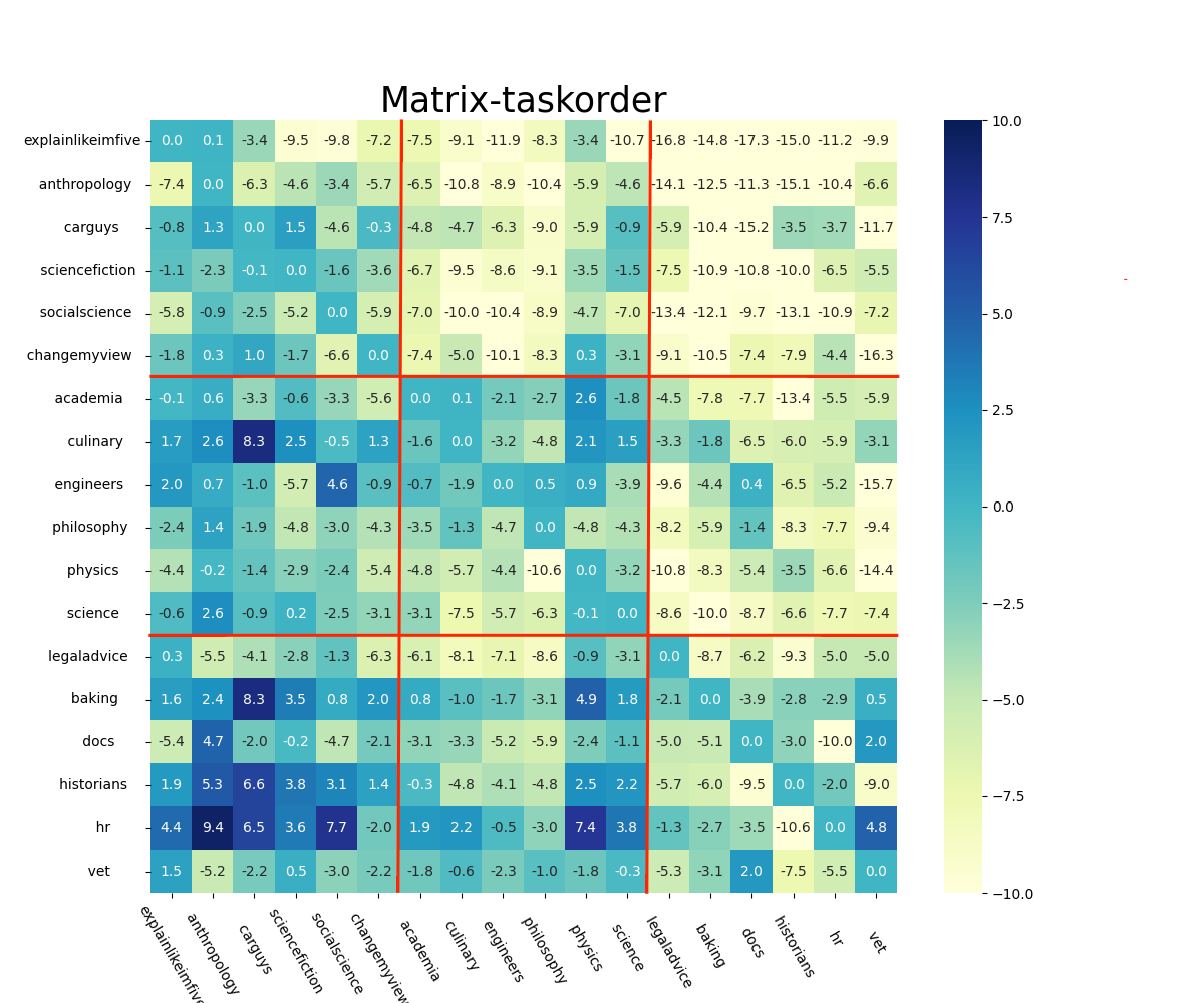
Figure 6: Enter Caption

References

- [1] Yuntao Bai, Andy Jones, Kamal Ndousse, Amanda Askell, Anna Chen, Nova DasSarma, Dawn Drain, Stanislav Fort, Deep Ganguli, Tom Henighan, Nicholas Joseph, Saurav Kadavath, Jackson Kernion, Tom Conerly, Sheer El-Showk, Nelson Elhage, Zac Hatfield-Dodds, Danny Hernandez, Tristan Hume, Scott Johnston, Shauna Kravec, Liane Lovitt, Neel Nanda, Catherine Olsson, Dario Amodei, Tom Brown, Jack Clark, Sam McCandlish, Chris Olah, Ben Mann, and Jared Kaplan. Training a helpful and harmless assistant with reinforcement learning from human feedback, 2022.
- [2] Nisan Stiennon, Long Ouyang, Jeff Wu, Daniel M. Ziegler, Ryan Lowe, Chelsea Voss, Alec Radford, Dario Amodei, and Paul F. Christiano. Learning to summarize from human feedback. CoRR, abs/2009.01325, 2020.
- [3] Long Ouyang, Jeff Wu, Xu Jiang, Diogo Almeida, Carroll L. Wainwright, Pamela Mishkin, Chong Zhang, Sandhini Agarwal, Katarina Slama, Alex Ray, John Schulman, Jacob Hilton, Fraser Kelton, Luke Miller, Maddie Simens, Amanda Askell, Peter Welinder, Paul Christiano, Jan Leike, and Ryan Lowe. Training language models to follow instructions with human feedback, 2022.
- [4] Rafael Rafailov, Archit Sharma, Eric Mitchell, Stefano Ermon, Christopher D Manning, and Chelsea Finn. Direct preference optimization: Your language model is secretly a reward model. In ICML 2023 Workshop The Many Facets of Preference-Based Learning, 2023.
- [5] Leo Gao, John Schulman, and Jacob Hilton. Scaling laws for reward model overoptimization, 2022.
- [6] Shaojie Jiang, Ruqing Zhang, Svitlana Vakulenko, and Maarten de Rijke. A simple contrastive learning objective for alleviating neural text degeneration, 2022.
- [7] Liyuan Wang, Xingxing Zhang, Hang Su, and Jun Zhu. A comprehensive survey of continual learning: Theory, method and application, 2023.
- [8] Kawin Ethayarajh, Yejin Choi, and Swabha Swayamdipta. Understanding dataset difficulty with -usable information. In Kamalika Chaudhuri, Stefanie Jegelka, Le Song, Csaba Szepesvari, Gang Niu, and Sivan Sabato, editors, Proceedings of the 39th International Conference on Machine Learning, volume 162 of Proceedings of Machine Learning Research, pages 5988–6008. PMLR, 17–23 Jul 2022.
- [9] Andrew L. Maas, Raymond E. Daly, Peter T. Pham, Dan Huang, Andrew Y. Ng, and Christopher Potts. Learning word vectors for sentiment analysis. In Proceedings of the 49th Annual Meeting of the Association for Computational Linguistics: Human Language Technologies, pages 142–150, Portland, Oregon, USA, June 2011. Association for Computational Linguistics.
- [10] Rajkumar Ramamurthy, Prithviraj Ammanabrolu, Kianté Brantley, Jack Hessel, Rafet Sifa, Christian Bauckhage, Hannaneh Hajishirzi, and Yejin Choi. Is reinforcement learning (not) for natural language processing?: Benchmarks, baselines, and building blocks for natural language policy optimization. 2022.
- [11] John Schulman, Filip Wolski, Prafulla Dhariwal, Alec Radford, and Oleg Klimov. Proximal policy optimization algorithms. CoRR, abs/1707.06347, 2017.
- [12] Yixin Liu, Pengfei Liu, Dragomir Radev, and Graham Neubig. BRIO: Bringing order to abstractive summarization. In Proceedings of the 60th Annual Meeting of the Association for Computational Linguistics (Volume 1: Long Papers), pages 2890–2903, Dublin, Ireland, May 2022. Association for Computational Linguistics.
- [13] Xue Bin Peng, Aviral Kumar, Grace Zhang, and Sergey Levine. Advantage-weighted regression: Simple and scalable off-policy reinforcement learning. arXiv preprint arXiv:1910.00177, 2019.
- [14] Daniel Brown, Russell Coleman, Ravi Srinivasan, and Scott Niekum. Safe imitation learning via fast bayesian reward inference from preferences. In International Conference on Machine Learning, pages 1165–1177. PMLR, 2020.
- [15] Paul F Christiano, Jan Leike, Tom Brown, Miljan Martic, Shane Legg, and Dario Amodei. Deep reinforcement learning from human preferences. Advances in neural information processing systems, 30, 2017.
- [16] Riad Akrour, Marc Schoenauer, and Michèle Sebag. April: Active preference learning-based reinforcement learning. In Machine Learning and Knowledge Discovery in Databases: European Conference, ECML PKDD 2012, Bristol, UK, September 24-28, 2012. Proceedings, Part II 23, pages 116–131. Springer, 2012.
- [17] Marc Schoenauer, Riad Akrour, Michele Sebag, and Jean-Christophe Souplet. Programming by feedback. In Eric P. Xing and Tony Jebara, editors, Proceedings of the 31st International Conference on Machine Learning, volume 32 of Proceedings of Machine Learning Research, pages 1503–1511, Bejing, China, 22–24 Jun 2014. PMLR.
- [18] W Bradley Knox, Stephane Hatgis-Kessell, Serena Booth, Scott Niekum, Peter Stone, and Alessandro Allievi. Models of human preference for learning reward functions. arXiv preprint arXiv:2206.02231, 2022.
- [19] Baolin Peng, Linfeng Song, Ye Tian, Lifeng Jin, Haitao Mi, and Dong Yu. Stabilizing rlhf through advantage model and selective rehearsal, 2023.
- [20] Tianhao Wu, Banghua Zhu, Ruoyu Zhang, Zhaojin Wen, Kannan Ramchandran, and Jiantao Jiao. Pairwise proximal policy optimization: Harnessing relative feedback for llm alignment, 2023.
- [21] Feifan Song, Bowen Yu, Minghao Li, Haiyang Yu, Fei Huang, Yongbin Li, and Houfeng Wang. Preference ranking optimization for human alignment, 2023.
- [22] Hanze Dong, Wei Xiong, Deepanshu Goyal, Yihan Zhang, Winnie Chow, Rui Pan, Shizhe Diao, Jipeng Zhang, Kashun Shum, and Tong Zhang. Raft: Reward ranked finetuning for generative foundation model alignment, 2023.
- [23] Zheng Yuan, Hongyi Yuan, Chuanqi Tan, Wei Wang, Songfang Huang, and Fei Huang. Rrhf: Rank responses to align language models with human feedback without tears, 2023.
- [24] Hao Liu, Carmelo Sferrazza, and Pieter Abbeel. Chain of hindsight aligns language models with feedback, 2023.
- [25] Michael Völske, Martin Potthast, Shahbaz Syed, and Benno Stein. TL;DR: Mining Reddit to learn automatic summarization. In Proceedings of the Workshop on New Frontiers in Summarization, pages 59–63, Copenhagen, Denmark, September 2017. Association for Computational Linguistics.
- [26] Victor Sanh, Lysandre Debut, Julien Chaumond, and Thomas Wolf. Distilbert, a distilled version of BERT: smaller, faster, cheaper and lighter. CoRR, abs/1910.01108, 2019.
- [27] James Kirkpatrick, Razvan Pascanu, Neil Rabinowitz, Joel Veness, Guillaume Desjardins, Andrei A. Rusu, Kieran Milan, John Quan, Tiago Ramalho, Agnieszka Grabska-Barwinska, Demis Hassabis, Claudia Clopath, Dharshan Kumaran, and Raia Hadsell. Overcoming catastrophic forgetting in neural networks. Proceedings of the National Academy of Sciences, 114(13):3521–3526, 2017.
- [28] Rahaf Aljundi, Francesca Babiloni, Mohamed Elhoseiny, Marcus Rohrbach, and Tinne Tuytelaars. Memory aware synapses: Learning what (not) to forget. In Vittorio Ferrari, Martial Hebert, Cristian Sminchisescu, and Yair Weiss, editors, Proceedings of the European Conference on Computer Vision (ECCV), pages 144–161, Cham, 2018. Springer International Publishing.
- [29] Arslan Chaudhry, Marc’Aurelio Ranzato, Marcus Rohrbach, and Mohamed Elhoseiny. Efficient lifelong learning with A-GEM. In 7th International Conference on Learning Representations, ICLR 2019, New Orleans, LA, USA, May 6-9, 2019. OpenReview.net, 2019.
- [30] David Lopez-Paz and Marc’Aurelio Ranzato. Gradient episodic memory for continual learning. In Isabelle Guyon, Ulrike von Luxburg, Samy Bengio, Hanna M. Wallach, Rob Fergus, S. V. N. Vishwanathan, and Roman Garnett, editors, Advances in Neural Information Processing Systems 30: Annual Conference on Neural Information Processing Systems 2017, December 4-9, 2017, Long Beach, CA, USA, pages 6467–6476, 2017.
- [31] Zhizhong Li and Derek Hoiem. Learning without forgetting. IEEE Trans. Pattern Anal. Mach. Intell., 40(12):2935–2947, dec 2018.
- [32] Rahaf Aljundi, Klaas Kelchtermans, and Tinne Tuytelaars. Task-free continual learning. In The IEEE Conference on Computer Vision and Pattern Recognition (CVPR), June 2019.
- [33] Pietro Buzzega, Matteo Boschini, Angelo Porrello, Davide Abati, and SIMONE CALDERARA. Dark experience for general continual learning: a strong, simple baseline. In H. Larochelle, M. Ranzato, R. Hadsell, M.F. Balcan, and H. Lin, editors, Advances in Neural Information Processing Systems, volume 33, pages 15920–15930. Curran Associates, Inc., 2020.
- [34] Arslan Chaudhry, Puneet K. Dokania, Thalaiyasingam Ajanthan, and Philip H. S. Torr. Riemannian walk for incremental learning: Understanding forgetting and intransigence. In Proceedings of the European Conference on Computer Vision (ECCV), 2018.
- [35] Arthur Douillard, Matthieu Cord, Charles Ollion, Thomas Robert, and Eduardo Valle. Podnet: Pooled outputs distillation for small-tasks incremental learning. In Computer Vision–ECCV 2020: 16th European Conference, Glasgow, UK, August 23–28, 2020, Proceedings, Part XX 16, pages 86–102. Springer, 2020.
- [36] Saihui Hou, Xinyu Pan, Chen Change Loy, Zilei Wang, and Dahua Lin. Learning a unified classifier incrementally via rebalancing. In Proceedings of the IEEE/CVF conference on computer vision and pattern recognition, pages 831–839, 2019.
- [37] Francisco M Castro, Manuel J Marín-Jiménez, Nicolás Guil, Cordelia Schmid, and Karteek Alahari. End-to-end incremental learning. In Proceedings of the European conference on computer vision (ECCV), pages 233–248, 2018.
- [38] Long-Ji Lin. Self-improving reactive agents based on reinforcement learning, planning and teaching. Mach. Learn., 8(3–4):293–321, May 1992.
- [39] Fan-Keng Sun, Cheng-Hao Ho, and Hung-Yi Lee. LAMOL: language modeling for lifelong language learning. In 8th International Conference on Learning Representations, ICLR 2020, Addis Ababa, Ethiopia, April 26-30, 2020. OpenReview.net, 2020.
- [40] Xialei Liu, Chenshen Wu, Mikel Menta, Luis Herranz, Bogdan Raducanu, Andrew D Bagdanov, Shangling Jui, and Joost van de Weijer. Generative feature replay for class-incremental learning. In Proceedings of the IEEE/CVF Conference on Computer Vision and Pattern Recognition Workshops, pages 226–227, 2020.
- [41] Khurram Javed and Martha White. Meta-learning representations for continual learning. In H. Wallach, H. Larochelle, A. Beygelzimer, F. d'Alché-Buc, E. Fox, and R. Garnett, editors, Advances in Neural Information Processing Systems, volume 32. Curran Associates, Inc., 2019.
- [42] Jhair Gallardo, Tyler L Hayes, and Christopher Kanan. Self-supervised training enhances online continual learning. arXiv preprint arXiv:2103.14010, 2021.
- [43] Sanket Vaibhav Mehta, Darshan Patil, Sarath Chandar, and Emma Strubell. An empirical investigation of the role of pre-training in lifelong learning, 2022.
- [44] Rujun Han, Xiang Ren, and Nanyun Peng. ECONET: Effective continual pretraining of language models for event temporal reasoning. In Proceedings of the 2021 Conference on Empirical Methods in Natural Language Processing, pages 5367–5380, Online and Punta Cana, Dominican Republic, November 2021. Association for Computational Linguistics.
- [45] Pablo Sprechmann, Siddhant M. Jayakumar, Jack W. Rae, Alexander Pritzel, Adrià Puigdomènech Badia, Benigno Uria, Oriol Vinyals, Demis Hassabis, Razvan Pascanu, and Charles Blundell. Memory-based parameter adaptation. In 6th International Conference on Learning Representations, ICLR 2018, Vancouver, BC, Canada, April 30 - May 3, 2018, Conference Track Proceedings. OpenReview.net, 2018.
- [46] Joan Serra, Didac Suris, Marius Miron, and Alexandros Karatzoglou. Overcoming catastrophic forgetting with hard attention to the task. In International conference on machine learning, pages 4548–4557. PMLR, 2018.
- [47] Sayna Ebrahimi, Franziska Meier, Roberto Calandra, Trevor Darrell, and Marcus Rohrbach. Adversarial continual learning. In Computer Vision–ECCV 2020: 16th European Conference, Glasgow, UK, August 23–28, 2020, Proceedings, Part XI 16, pages 386–402. Springer, 2020.
- [48] Andrei A Rusu, Neil C Rabinowitz, Guillaume Desjardins, Hubert Soyer, James Kirkpatrick, Koray Kavukcuoglu, Razvan Pascanu, and Raia Hadsell. Progressive neural networks. arXiv preprint arXiv:1606.04671, 2016.
- [49] W. Bradley Knox and Peter Stone. Tamer: Training an agent manually via evaluative reinforcement. In 2008 7th IEEE International Conference on Development and Learning, pages 292–297, 2008.
- [50] James MacGlashan, Mark K. Ho, Robert Loftin, Bei Peng, Guan Wang, David L. Roberts, Matthew E. Taylor, and Michael L. Littman. Interactive learning from policy-dependent human feedback. In Doina Precup and Yee Whye Teh, editors, Proceedings of the 34th International Conference on Machine Learning, volume 70 of Proceedings of Machine Learning Research, pages 2285–2294. PMLR, 06–11 Aug 2017.
- [51] Paul F Christiano, Jan Leike, Tom Brown, Miljan Martic, Shane Legg, and Dario Amodei. Deep reinforcement learning from human preferences. In I. Guyon, U. Von Luxburg, S. Bengio, H. Wallach, R. Fergus, S. Vishwanathan, and R. Garnett, editors, Advances in Neural Information Processing Systems, volume 30. Curran Associates, Inc., 2017.
- [52] Garrett Warnell, Nicholas Waytowich, Vernon Lawhern, and Peter Stone. Deep tamer: Interactive agent shaping in high-dimensional state spaces. In Proceedings of the Thirty-Second AAAI Conference on Artificial Intelligence and Thirtieth Innovative Applications of Artificial Intelligence Conference and Eighth AAAI Symposium on Educational Advances in Artificial Intelligence, AAAI’18/IAAI’18/EAAI’18. AAAI Press, 2018.
- [53] Jérémy Scheurer, Jon Ander Campos, Tomasz Korbak, Jun Shern Chan, Angelica Chen, Kyunghyun Cho, and Ethan Perez. Training language models with language feedback at scale, 2023.
- [54] Yuntao Bai, Saurav Kadavath, Sandipan Kundu, Amanda Askell, Jackson Kernion, Andy Jones, Anna Chen, Anna Goldie, Azalia Mirhoseini, Cameron McKinnon, Carol Chen, Catherine Olsson, Christopher Olah, Danny Hernandez, Dawn Drain, Deep Ganguli, Dustin Li, Eli Tran-Johnson, Ethan Perez, Jamie Kerr, Jared Mueller, Jeffrey Ladish, Joshua Landau, Kamal Ndousse, Kamile Lukosuite, Liane Lovitt, Michael Sellitto, Nelson Elhage, Nicholas Schiefer, Noemi Mercado, Nova DasSarma, Robert Lasenby, Robin Larson, Sam Ringer, Scott Johnston, Shauna Kravec, Sheer El Showk, Stanislav Fort, Tamera Lanham, Timothy Telleen-Lawton, Tom Conerly, Tom Henighan, Tristan Hume, Samuel R. Bowman, Zac Hatfield-Dodds, Ben Mann, Dario Amodei, Nicholas Joseph, Sam McCandlish, Tom Brown, and Jared Kaplan. Constitutional ai: Harmlessness from ai feedback, 2022.
- [55] Ethan Perez, Saffron Huang, Francis Song, Trevor Cai, Roman Ring, John Aslanides, Amelia Glaese, Nat McAleese, and Geoffrey Irving. Red teaming language models with language models. In Proceedings of the 2022 Conference on Empirical Methods in Natural Language Processing, pages 3419–3448, Abu Dhabi, United Arab Emirates, December 2022. Association for Computational Linguistics.
- [56] Deep Ganguli, Liane Lovitt, Jackson Kernion, Amanda Askell, Yuntao Bai, Saurav Kadavath, Ben Mann, Ethan Perez, Nicholas Schiefer, Kamal Ndousse, Andy Jones, Sam Bowman, Anna Chen, Tom Conerly, Nova DasSarma, Dawn Drain, Nelson Elhage, Sheer El-Showk, Stanislav Fort, Zac Hatfield-Dodds, Tom Henighan, Danny Hernandez, Tristan Hume, Josh Jacobson, Scott Johnston, Shauna Kravec, Catherine Olsson, Sam Ringer, Eli Tran-Johnson, Dario Amodei, Tom Brown, Nicholas Joseph, Sam McCandlish, Chris Olah, Jared Kaplan, and Jack Clark. Red teaming language models to reduce harms: Methods, scaling behaviors, and lessons learned, 2022.
- [57] Róbert Busa-Fekete, Balázs Szörényi, Paul Weng, Weiwei Cheng, and Eyke Hüllermeier. Preference-based reinforcement learning: evolutionary direct policy search using a preference-based racing algorithm. Machine learning, 97:327–351, 2014.
- [58] Aadirupa Saha, Aldo Pacchiano, and Jonathan Lee. Dueling rl: Reinforcement learning with trajectory preferences. In International Conference on Artificial Intelligence and Statistics, pages 6263–6289. PMLR, 2023.
- [59] Ashesh Jain, Brian Wojcik, Thorsten Joachims, and Ashutosh Saxena. Learning trajectory preferences for manipulators via iterative improvement. Advances in neural information processing systems, 26, 2013.
- [60] Paul F Christiano, Jan Leike, Tom Brown, Miljan Martic, Shane Legg, and Dario Amodei. Deep reinforcement learning from human preferences. Advances in neural information processing systems, 30, 2017.
- [61] Dorsa Sadigh, Anca D Dragan, Shankar Sastry, and Sanjit A Seshia. Active preference-based learning of reward functions. 2017.
- [62] Andras Kupcsik, David Hsu, and Wee Sun Lee. Learning dynamic robot-to-human object handover from human feedback. Robotics Research: Volume 1, pages 161–176, 2018.