Physics-Informed with Power-Enhanced Residual Network for Interpolation and Inverse Problems

Abstract

This paper introduces a novel neural network structure called the Power-Enhancing residual network, designed to improve interpolation capabilities for both smooth and non-smooth functions in 2D and 3D settings. By adding power terms to residual elements, the architecture boosts the network’s expressive power. The study explores network depth, width, and optimization methods, showing the architecture’s adaptability and performance advantages. Consistently, the results emphasize the exceptional accuracy of the proposed Power-Enhancing residual network, particularly for non-smooth functions. Real-world examples also confirm its superiority over plain neural network in terms of accuracy, convergence, and efficiency. The study also looks at the impact of deeper network. Moreover, the proposed architecture is also applied to solving the inverse Burgers’ equation, demonstrating superior performance. In conclusion, the Power-Enhancing residual network offers a versatile solution that significantly enhances neural network capabilities. The codes implemented are available at: https://github.com/CMMAi/ResNet_for_PINN.

1 Introduction

Deep neural networks have revolutionized the field of machine learning and artificial intelligence, achieving remarkable success in various applications, including image recognition, natural language processing, and reinforcement learning. Moreover, their adaptability extends beyond these domains, as evidenced by their effective integration with physics-informed approaches [1]. One significant development in this domain was the introduction of residual networks, commonly known as ResNets [2, 3], which demonstrated unprecedented performance in constructing deep architectures and mitigating the vanishing gradient problem. ResNets leverage skip connections to create shortcut paths between layers, resulting in a smoother loss function. This permits efficient gradient flow, thus enhancing training performance across various sizes of neural networks [4]. Our research aligns closely with theirs, particularly in our exploration of skip connections’ effects on loss functions. In 2016, Veit et al. [5] unveiled a new perspective on ResNet, providing a comprehensive insight. Velt’s research underscored the idea that residual networks could be envisioned as an assembly of paths with varying lengths. These networks effectively employed shorter paths for training, effectively resolving the vanishing gradient problem and facilitating the training of exceptionally deep models. Jastrzębski et al.’s research [6] highlighted Residual Networks’ iterative feature refinement process numerically. Their findings emphasized how residual connections guided features along negative gradients between blocks, and show that effective sharing of residual layers mitigates overfitting.

In related engineering work, Lu et al. [7] leveraged recent neural network progress via a multifidelity (MFNN) strategy (MFNN: refers to a neural network architecture that combines outputs from multiple models with varying levels of fidelity or accuracy) for extracting material properties from instrumented indentation (see [7], Fig. 1(D) ). The proposed MFNN in this study incorporates a residual link that connects the low-fidelity output to the high-fidelity output at each iteration, rather than between layers. Wang et al. [8] proposed an improved fully-connected neural architecture. The key innovation involves integrating two transformer networks to project input variables into a high-dimensional feature space. This architecture combines multiplicative interactions and residuals, resulting in improved predictive accuracy, but with the cost of CPU time.

In this paper, we propose a novel architecture called the Power-Enhancing SkipResNet, aimed at advancing the interpolation capabilities of deep neural networks for smooth and non-smooth functions in 2D and 3D domains. The key objectives of this research are as follows:

• Introduces the “Power-Enhancing SkipResNet” architecture.

• Enhances network’s expressive power for improved accuracy and convergence.

• Outperforms conventional plain neural networks.

• Conducts extensive experiments on diverse interpolation scenarios and inverse Burger’s equation.

• Demonstrates benefits of deeper architectures.

Through rigorous analysis and comparisons, we demonstrate the advantages of the proposed architecture in terms of accuracy and convergence speed.

The remainder of this paper is organized as follows: Section 2 reviews the neural network and its application for solving interpolation problems. In Section 3, we briefly presents physics informed neural network for solving inverse Burgers’ equation. Section 4 discusses the residual network and the proposed Power-Enhancing SkipResNet, explaining the incorporation of power terms and its potential benefits. Section 5 presents the experimental setup and the evaluation of results and discusses the findings. Finally, Section 6 concludes the paper with a summary of contributions and potential future research directions.

2 Neural Networks

In this section, we will explore the utilization of feedforward neural networks for solving interpolation problems, specifically focusing on constructing accurate approximations of functions based on given data points.

2.1 Feedforward Neural Networks

The feedforward neural network, also known as a multilayer perceptron (MLP), serves as a foundational architecture in artificial neural networks. Comprising interconnected layers of neurons, the information flow progresses unidirectionally from the input layer through hidden layers to the output layer. This process, termed “feedforward,” entails transforming input data into desired output predictions. The core constituents of a feedforward neural network are its individual neurons. A neuron computes a weighted sum of its inputs, augmented by a bias term, before applying an activation function to the result.

For a neuron with $n$ number of inputs (data points) in the given layer $i$, where inputs are denoted as $\mathcal{X}=[{\rm{x}}_{1},{\rm{x}}_{2},\ldots,{\rm{x}}_{n}]$, weights as $\mathbf{w}=[w_{1},w_{2},\ldots,w_{n}]$, and bias $b_{i}$, the output $z_{i}$ is computed as:

$$z_{i}=\sum_{j=1}^{n}w_{j}{\rm{x}}_{j}+b_{i}$$ (1)

where $\rm{x}_{j}$ has a dimension of $d$ such that ${\rm{x}}=(x_{1},x_{2},\ldots,x_{d})$. The output is then transformed using an activation function $h(\cdot)$:

$$y_{i}=h(z_{i})$$ (2)

It is important to note that while hidden layers utilize activation functions to introduce non-linearity, the last layer (output layer) typically does not apply an activation function to its outputs.

2.2 Neural Networks for Interpolation

In the context of interpolation problems, feedforward neural networks can be leveraged to approximate functions based on a given set of data points. The primary objective is to construct a neural network capable of accurately predicting function values at points not explicitly included in the provided dataset.

2.2.1 Training Process

The training of the neural network involves adjusting its weights and biases to minimize the disparity between predicted outputs and actual data values. This optimization process is typically driven by algorithms such as gradient descent, which iteratively update network parameters to minimize a chosen loss function.

2.2.2 Loss Function for Interpolation

In interpolation tasks, the selection of an appropriate loss function is crucial. One common choice is the mean squared error (MSE), which quantifies the discrepancies between predicted values, denoted as $N$, and the true data values, denoted as $u$, at each data point, represented as ${{\rm{x}}_{j}}$. The MSE is calculated over a total of $n$ data points using the formula:

$$MSE=\frac{1}{n}\sum^{n}_{j=1}(u({\rm{x}}_{j})-N({\rm{x}}_{j}))^{2}$$ (3)

This loss function guides the optimization process, steering the network toward producing accurate predictions.

3 PINN for Solving Inverse Burgers’ Equation

In this section, we explore the application of Physics-Informed Neural Networks (PINN) [1] to solve the inverse Burgers’ equation in one dimension. The 1D Burgers’ equation is given by:

$$\frac{\partial u}{\partial t}+\lambda_{1}u\frac{\partial u}{\partial x}=\lambda_{2}\frac{\partial^{2}u}{\partial x^{2}}$$ (4)

where $u({\rm x})=u(x,t)$ is the solution, and $\lambda_{1}$ and $\lambda_{2}$ are coefficients to be determined. Here, $x\in[-1,1]$ and $t\in[0,1]$ represent two dimensions, space and time respectively.

In the context of solving the inverse Burgers’ equation, we combine the power of neural networks (Fig. 1(I)) with the physical governing equation (Fig. 1(II)) to form PINN. Utilizing the universal approximation theorem, we approximate the solution $N(x,t)\approx u(x,t)$. By automatically differentiating the network, we can compute derivatives such as $N_{t}=\frac{\partial N}{\partial t}$, $N_{xx}=\frac{\partial^{2}N}{\partial x^{2}}$, etc. We define the function $g(x,t)$ representing the residual of the Burgers’ equation as:

$$g(x,t)=N_{t}+\lambda_{1}NN_{x}-\lambda_{2}N_{xx}$$ (5)

The PINNs loss function is given by (Fig. 1(II)):

$$MSE_{g}=\frac{1}{n_{c}}\sum^{n_{c}}_{i=1}(g(x^{i},t^{i}))^{2}$$ (6)

where $n_{c}$ is the number of collocation points and pairs of $(x,t)$ specify the space and time values. In this inverse problem, we know the true data, so we compute the loss with respect to the reference solution as well (Fig. 1(I)):

$$MSE_{u}=\frac{1}{n}\sum^{n}_{j=1}\left(u(x^{i},t^{i})-N(x^{j},t^{j})\right)^{2}$$ (7)

where $n$ represents the number of data locations. The total loss function minimized during training is:

$$MSE=MSE_{u}+MSE_{g}$$ (8)

We aim to minimize $MSE$ to obtain the neural network parameters $(\mathbf{w},b_{i})$ and the Burgers’ equation parameters $\lambda_{1}$ and $\lambda_{2}$.

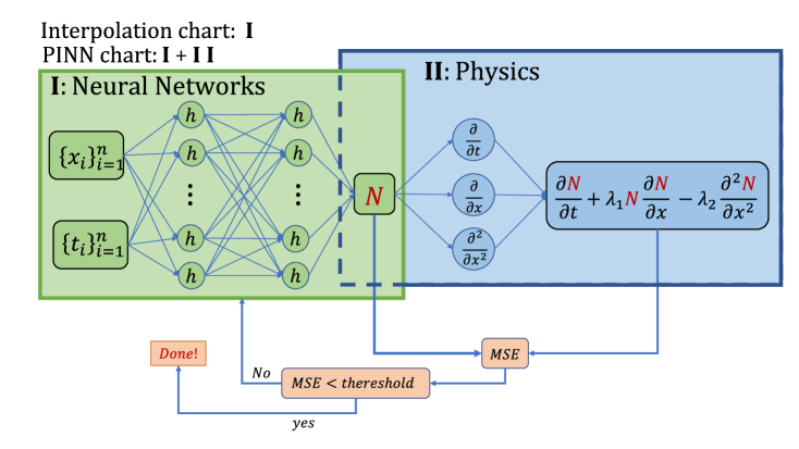
Figure 1: The neural network (interpolation stage) + physics (inverse Burger’s equation). Here, $x$ and $t$ represent two dimensions, each including $n$ examples.

4 Residual Network

Residual networks, commonly referred to as ResNets [2, 3], have become a prominent architecture in neural networks. They are characterized by their residual modules, denoted as $f_{i}$, and skip connections that bypass these modules, enabling the construction of deep networks. This allows for the creation of residual blocks, which are sets of layers within the network. In contrast with Fig. 2(a), which illustrates the plain neural network, Fig. 2(b) showcases the network architecture incorporating ResNet features. To simplify notation, the initial pre-processing and final steps are excluded from our discussion. Therefore, the definition of the output $y_{i}$ for the $i$-th layer is given as follows:

$$y_{i}=f_{i}(y_{i-1})+y_{i-1}.$$ (9)

Here, $f_{i}(x)$ encompasses a sequence of operations, including linear transformations (1), element-wise activation functions (2), and normalization techniques.

In this study, we propose a power-enhanced variant of the ResNet that skips every other layer, denoted as the “Power-Enhanced SkipResNet.” The modification involves altering the recursive definition in (9) as follows:

$$\left\{\begin{aligned} y_{i}&=f_{i}(y_{i-1})+y^{p}_{i-1},&\text{for}\quad i=1,3,5,\ldots\\ y_{i}&=f_{i}(y_{i-1}),&\text{for}\quad i=2,4,6,\ldots\end{aligned}\right.$$ (10)

This novel configuration, illustrated in Fig. 2(c), introduces the use of a power term $y^{p}_{i-1}$ for specific layers, enhancing the expressive power of the network.

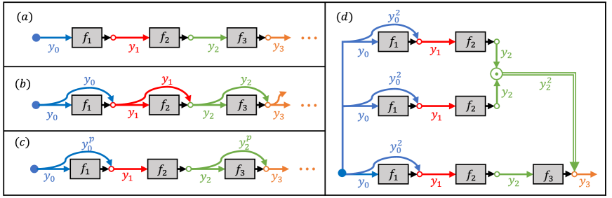
Figure 2: Three neural network architectures: (a) plain neural network (Plain NN), (b) residual network (ResNet), (c) power-enhanced SkipResNet, and (d) Unraveled SQR-SkipResNet (plot (c) with $p=2$) where $\odot$ denotes element-wise multiplication.

For the purpose of comparison among Plain NN, ResNet, and SQR-SkipResNet (Figs. 2(a)-(c), respectively), we evaluate the output of the third hidden layer concerning the input $y_{0}=\mathcal{X}$. The results for the plain neural network are as follows:

$$y_{3} =f_{3}(y_{2})$$

$$=f_{3}(f_{2}(y_{1}))$$

$$=f_{3}(f_{2}(f_{1}(y_{0})))$$ (11)

Meanwhile, the corresponding ResNet formulation is as follows [5]:

$$y_{3} =f_{3}(y_{2})+y_{2}$$

$$=f_{3}(f_{2}(y_{1})+y_{1})+\left[f_{2}(y_{1})+y_{1}\right]$$

$$=f_{3}(f_{2}(f_{1}(y_{0})+y_{0})+f_{1}(y_{0})+y_{0})+\left[f_{2}(f_{1}(y_{0})+y_{0})+f_{1}(y_{0})+y_{0}\right]$$ (12)

Finally, the formulation of the first three hidden layers for the SQR-SkipResNet is as follows:

$$y_{3} =f_{3}(y_{2})+y_{2}^{p}$$

$$=f_{3}(f_{2}(y_{1}))+\left[f_{2}(y_{1})\right]^{p}$$

$$=f_{3}(f_{2}(f_{1}(y_{0})+y_{0}^{p}))+\left[f_{2}(f_{1}(y_{0})+y_{0}^{p})\right]^{p}$$ (13)

Figure 2(d) visually represents the “expression tree” for the case with $p=2$, providing an insightful illustration of the data flow from input to output. The graph demonstrates the existence of multiple paths that the data can traverse. Each of these paths represents a distinct configuration, determining which residual modules are entered and which ones are skipped.

Our extensive numerical experiments support our approach, indicating that a power of 2 is effective for networks with fewer than 30 hidden layers. However, for deeper networks, a larger power can contribute to network stability. Nonetheless, deploying such deep networks does not substantially enhance accuracy and notably increases CPU time. In tasks like interpolation and solving PDEs, a power of 2 generally suffices, and going beyond may not justify the added complexity in terms of accuracy and efficiency

5 Numerical Results

In this study, we employ the notations $n$, $n_{l}$, and $n_{n}$ to represent the number of data points (training), layers, and neurons in each layer, respectively. In all following examples, unless otherwise mentioned, we consider $100^{2}$ validation data points. We also introduce three distinct types of error measurements between exact $u$ and approximated $N$ solutions:

1. Mean Square Error: The training errors shown in the plotted graphs, relative to the iteration number, are computed using the mean square error criterion.
   

   $$\text{Mean Square Error}=\frac{1}{n}\sum_{i=1}^{n}\left({u}_{i}-{N}_{i}\right)^{2}$$

2. Relative L2 Norm Error: The validation errors, calculated over the test data and presented in the plotted graphs concerning the iteration number, are measured using the relative L2 norm error metric.
   

   $$\text{Relative L2 Norm Error}=\frac{\|{u}-{N}\|_{2}}{\|{u}\|_{2}}$$

3. Maximum Absolute Error: When visualizing errors across the entire domain, whether in 2D or 3D scenarios, the error represented on the contour error plot is referred to as the maximum absolute error. It is important to note that the contour bars are scaled according to the largest error in the plot.
   

   $$\text{Maximum Absolute Error}=\max\left|{u}-{N}\right|$$

These error metrics provide valuable insights into the accuracy and convergence of the methods used in this study. In this section four methods will be investigated.

1. Plain NN: A conventional neural network without any additional modifications or residual connections (see Fig. 2(a)).

2. ResNet: A residual neural network architecture where the output of each layer is obtained by adding the residual to the layer’s output (see Fig. 2(b)).

3. SkipResNet: An extension of ResNet, where the residual connection is applied every other layer, alternating between including and excluding the residual connection (see Fig. 2(c) where $p=1$).

4. SQR-SkipResNet: An innovative variation of the ResNet architecture, where the squared residual is added every other layer. In this approach, the output of each alternate layer is obtained by squaring the previous layer’s output and adding the squared residual to it (see Fig. 2(c)-(d) where $p=2$).

In all our experiments, we primarily employ L-BFGS-B (Limited-memory Broyden-Fletcher-Goldfarb-Shanno with Box constraints) and occasionally, for comparison, we also use Adam (Adaptive Moment Estimation). Convergence, particularly with L-BFGS-B optimization, is identified by satisfying preset tolerance levels for gradient or function value change, or by reaching the defined maximum number of iterations, with a gradient tolerance of $1\times 10^{-9}$, and a change in function value tolerance of $1\times 10^{-9}$.

The numerical experiments were executed on a computer equipped with an Intel(R) Core(TM) i9-9900 CPU operating at 3.10GHz with a total of 64.0 GB of RAM.

Example 1

For the first example, three test functions are investigated and depicted in Fig. 3. The top panel of Fig. 3 displays the 3D surface plot of the test functions, while the bottom panel presents the corresponding contour plots. F1 is a smooth function, originally introduced by Franke [9], which has been extensively used for studying radial basis function (RBF) interpolation. On the other hand, F2 and F3 are non-smooth functions [10].

$${{\rm F1}(x_{1},x_{2})} =\frac{3}{4}\exp\left[\frac{-1}{4}\left((9x_{1}-2)^{2}+(9x_{2}-2)^{2}\right)\right]+\frac{3}{4}\exp\left[\frac{-1}{49}(9x_{1}+1)^{2}-\frac{1}{10}(9x_{2}+1)^{2}\right]$$

$$+\frac{1}{2}\exp\left[\frac{-1}{4}\left((9x_{1}-7)^{2}+(9x_{2}-3)^{2}\right)\right]-\frac{1}{5}\exp\left[-(9x_{1}-4)^{2}-(9x_{2}-7)^{2}\right],$$

$${{\rm F2}(x_{1},x_{2})} =\frac{0.0025}{(x_{1}-1.01)^{2}+(x_{2}-1.01)^{2}},$$

$${{\rm F3}(x_{1},x_{2})} =\frac{1}{9}\left[64-81\left(\left|x_{1}-\frac{1}{2}\right|+\left|x_{2}-\frac{1}{2}\right|\right)\right]-\frac{1}{2}.$$

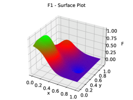
(a) F1

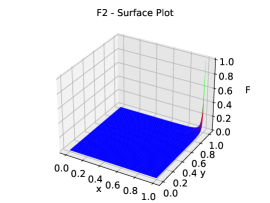
(b) F2

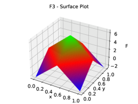
(c) F3

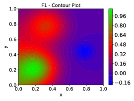
(d) F1

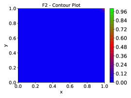
(e) F2

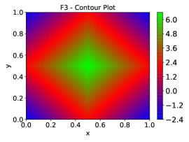
(f) F3

Figure 3: The profile of the F1, F2, and F3

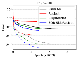
(a) $n=500$

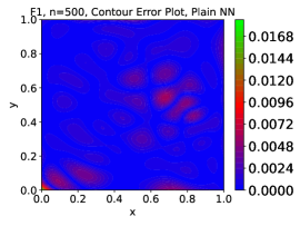
(b) Plain NN

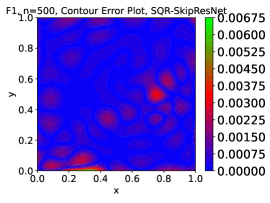
(c) SQR-SkipResNet

Figure 4: The profiles of training on F1 for different number of collocation points $n$. Dotted-line curves denote training error, and solid-line curves denote validation error.

First we investigate the performance of four neural networks: Plain NN, ResNet, SkipResNet, and SQR-SkipResNet. The entire analysis is based on the network with $n_{l}=10$, and each layer contains 50 neurons ($n_{n}$). Figure. 4 shows the results of interpolation using $500$ training data and $100^{2}$ validation data. Figure 4(a) presents the Mean Squared Error (MSE) over training (dashed line) and Relative L2 Norm over validation (solid line) data points. Figure 4(b)-4(c) show the maximum absolute errors for Plain NN and SQR-SkipResNet, respectively.

Our observations from these plots are as follows:

1. Plot (a) indicates that the ResNet is not accurate enough compared to the other three networks, both during training and validation. This pattern has been consistently observed in various examples, and we will no longer investigate the ResNet performance.

2. As indicated by the plot, it can be observed that the Plain NN necessitates approximately 2400 iterations for convergence, whereas the proposed SQR-SkipResNet achieves convergence in a significantly reduced 1400 iterations. Additionally, the latter method exhibits higher accuracy compared to the former.

3. Plot (a) also shows that SkipResNet performs somewhat between Plain NN and SQR-SkipResNet. This behavior has been observed in different examples conducted by the authors, but we do not plan to further investigate this method.

4. Contour error plots for both Plain NN and SQR-SkipResNet are presented in plots (b) and (c) respectively. These plots highlight that the maximum absolute error achieved with SQR-SkipResNet exhibits a remarkable improvement of approximately 60% compared to Plain NN.

Therefore, a higher accuracy and better convergence are observed when using SQR-SkipResNet compared to other algorithms.

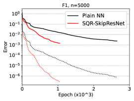
(a) $n=5000$

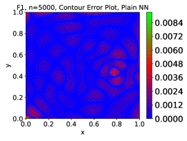
(b) Plain NN

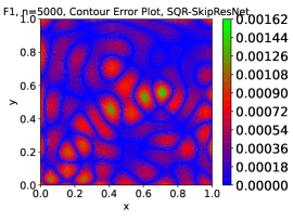
(c) SQR-SkipResNet

Figure 5: Example 1: The profiles of (a) training and validation results on F1 with 5000 data points. Dotted-line curves denote training error, and solid-line curves denote validation error. The corresponding contour error plots for (b) the plain NN and (c) SQR-SkipResNet.

Fig. 5 illustrates the outcomes obtained through the utilization of a large number of data points, $n=5000$, employed for the interpolation of F1. A better convergence from Fig. 5(a) can be observed using the proposed SQR-SkipResNet compared to Plain NN. The Plain NN yields a maximum absolute error of $9.07\times 10^{-3}$ in 113 seconds, whereas the proposed SQR-SkipResNet approach achieves a significantly reduced error of $1.56\times 10^{-3}$ in only 55 seconds, shown in Fig. 5(b)-5(c), respectively. This represents an improvement of approximately $82.8\%$ in terms of error reduction and a substantial $51.3\%$ reduction in CPU processing time. A comparison between Fig. 4(a) and Fig. 5(a) reveals that a greater number of data values results in an improved convergence rate for the proposed SQR-SkipResNet, whereas the Plain NN exhibits a slightly higher iteration number.

More investigations on the performance of the SQR-SkipResNet has been done by interpolating the non-smooth functions F2 and F3. Figure 6 presents the interpolation results for F2 on the top panel and F3 on the bottom panel with $n=1000$. The corresponding training and validation error with respect to the epoch are shown in the first column. The second and third columns show the interpolated surface using Plain NN and SQR-SkipResNet, respectively. Clearly, a better surface interpolation has been carried using the proposed method. More details are listed in Table 1. This table shows that the accuracy using the SQR-SkipResNet is slightly better than Plain NN, however it is worth nothing that these functions are non-smooth and a slightly changes in error would affect the quality of interpolation tremendously as shown in Fig. 6. However to reach a better accuracy, the SQR-SkipResnet requires larger number of iterations and consequently the higher CPU time. This can be seen as the trade-off that SQR-SkipResNet makes for interpolating non-smooth functions to obtain better accuracy, in contrast to the smaller CPU time it requires for interpolating smooth functions.

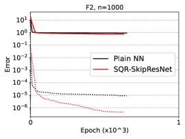
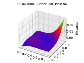
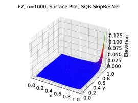
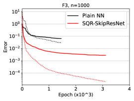
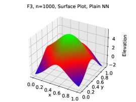
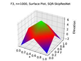
Figure 6: Example 1: The profile of the F2, and F3

Table 1: Example 1: Maximum absolute errors and CPU time (t) for F2-F3.

function	Plain NN		SQR-SkipResNet
	error	t(s)	error	t(s)
F2	9.71e-01	22	8.59e-01	27
F3	7.98e-01	51	8.57e-02	132

Example 2

In this example, we demonstrate the performance of the proposed method in a real case study. Specifically, we interpolate the Mt. Eden or Maungawhau volcano in Auckland, NZ, as depicted in Fig. 7 [11]. The available data consists of 5307 elevation points uniformly distributed in a mesh grid area of size 10 by 10 meters. Plot (b) shows the 3D surface, and plot (c) presents the contour plot of the volcano.

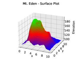
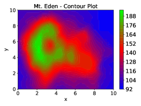
Figure 7: Example 2: (a) An image showcasing the Mt. Eden or Maungawhau volcano located in Auckland, New Zealand [11]. (b) A 3D surface representation generated from a dataset containing $n=5307$ data points. (c) A contour plot providing insights into the topography of Mt. Eden.

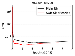
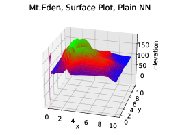
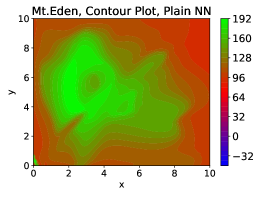
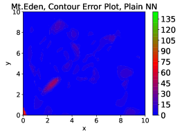
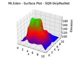
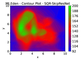
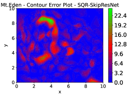
Figure 8: Example 2: Maximum absolute error for Mt. Eden interpolation using L-BFGS-B optimizer with $n=200$, $n_{n}=50$, and $n_{l}=5$.

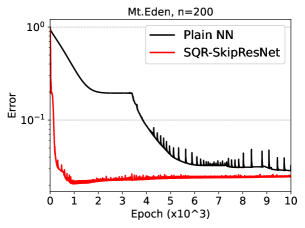
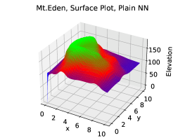
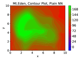
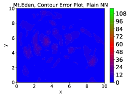
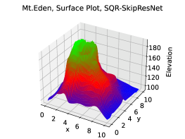
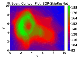
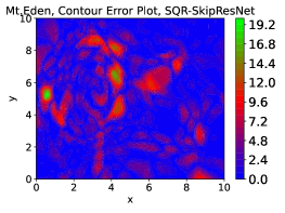
Figure 9: Example 2: Mt. Eden interpolation results using Adam optimizer with $n=200$, $n_{n}=50$, and $n_{l}=5$.

In the first experiment, we utilize only 200 collocation points, 5 hidden layers with $n_{n}=100$, and we optimize the training using L-BFGS-B. The remaining data, 5107 data points, are used for validation. The results are shown in Fig. 8, which illustrates the relative L2 norm error over the test data. Evidently, SQR-SkipResNet achieves higher accuracy with fewer iterations. The convergence time for SQR-SkipResNet is 68 seconds, and it requires 4600 iterations to converge. On the other hand, Plain NN requires 80 seconds and 5600 iterations to achieve convergence.

Additionally, we provide more details on the interpolated surface and accuracy in Fig. 8. The second row shows the interpolated surface using Plain NN, while the third row shows the results obtained with SQR-SkipResNet. Specifically, plots 8(b) and 8(e) depict the interpolated surfaces for Plain NN and SQR-SkipResNet, respectively. Similarly, plots 8(c) and 8(f) display the contour plots for both methods. Finally, plots 8(d) and 8(g) represent the contour error plots, measured by the maximum absolute error, for Plain NN and SQR-SkipResNet, respectively.

Clearly, the results using SQR-SkipResNet significantly outperform those from Plain NN. The accuracy of Plain NN, specifically in terms of the maximum absolute error, improves significantly (500%) when using the SQR-SkipResNet architecture. This underscores the superiority of SQR-SkipResNet in achieving more accurate and reliable interpolation results.

Table 2: Example 2: Maximum absolute errors (m) for Mt. Eden interpolation using Adam optimizer for various number of training data points $n$, neurons $n_{n}$ and layers $n_{l}$.

$n$	$n_{n}$	$n_{l}$	Plain NN	SQR-SkipResNet
200	50	5	✗	12.9
		10	✗	32.6
	100	5	114	19.6
		10	✗	25.5
1000	50	5	21.6	4.77
		10	✗	14.0
	100	5	7.36	6.28
		10	✗	7.78

In our second experiment, we repeat the the previous example but this time we use Adam optimizer with the learning rate of 1.0E-3, and 10k iteration. The organization of plots are as the previous example. Plot 9(a) shows that SQR-SkipResNet works much more accurate from the beginning of the iterations with much less fluctuation compare with Plain NN (compare plots 9 (b) and 9(e), respectively, and its corresponding contour plots in 9(c) and 9(f)). We also see that the interpolated surface when using the SQR-SkipResNet (plot 9(g)) can be completely better than Plain NN (plot 9(d)). The accuracy with respect to the maximum absolute error for the latter one is about 462% better than the Plain NN. A comparisopn between these two optimizers, L-BFGS-B (Fig. 8 and Fig. 9) shows a better performance using Adam for both Plain NN and proposed SQR-SkipResNet.

Therefore, we further investigate the impact of the number of data points $n$, neurons $n_{n}$, and layers $n_{l}$ as listed in Table 2. In this table, ✗ denotes cases where training failed. When training fails, the interpolated surface remains partly flat and partly non-smooth. we have the following observations:

• As $n$ increases, smaller errors obtained.

• With a fixed number of neurons $n_{n}$, the errors are smaller when the number of layers is $n_{l}=5$ compared to $n_{l}=10$.

• With a fixed number of layers $n_{l}$, the errors are smaller when the number of neurons is $n_{n}=50$ compared to $n_{n}=100$.

• Plain NN failed to train in 5 cases, while the proposed method exhibited successful performance.

Finally we see that in all cases, SQR-SkipResNet led to better accuracy compare to Plain NN.

Example 3

In the concluding example regarding the interpolation problems, we analyze the effectiveness of the proposed neural network in a 3D example, specifically using the Stanford bunny model, as depicted in Fig. 10. The entire bunny model has been scaled by a factor of 10. A distribution of points over the bunny’s surface is illustrated in Fig. 10, comprising a total of 8171 data points. The validation error is performed using the following test function (refer to [12], F4):

$${\rm F4}(x_{1},x_{2},x_{3})=\frac{1}{3}\exp\left[-\frac{81}{16}\left((x_{1}-0.5)^{2}+(x_{2}-0.5)^{2}+(x_{3}-0.5)^{2}\right)\right]$$

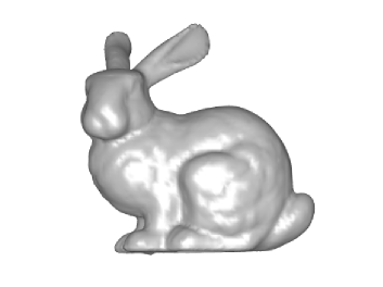
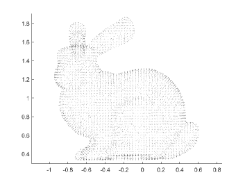
Figure 10: Example 3: The Stanford Bunny.

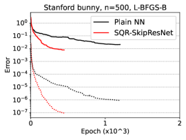
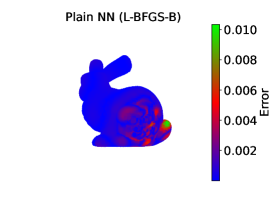
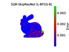
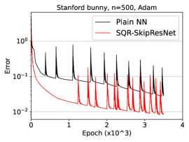
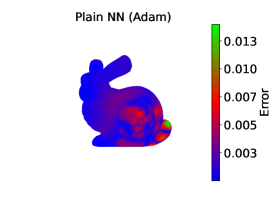
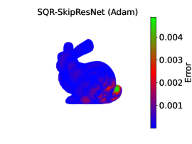
Figure 11: Example 3: Error profile comparison for the Stanford Bunny model using L-BFGS-B (top panel) and Adam optimizers (bottom panel). Training errors are indicated by the dotted line, and validation errors are represented by the solid line.

In Fig. 11, the training process (dotted line) is depicted with 500 data values, while the remaining 7671 points are reserved for validation error assessment (solid line). The top panel showcases results obtained using the L-BFGS-B optimizer, while the bottom panel displays outcomes achieved through the Adam optimizer. As demonstrated in Fig. 11, the SQR-SkipResNet surpasses the Plain NN in terms of accuracy and convergence rate across both the training and test datasets. The recorded CPU times amount to 35 seconds for Plain NN and 15 seconds for SQR-SkipResNet. Plots (b) and (c) offer insight into the maximum absolute error, highlighting an accuracy improvement of approximately 70% when implementing the proposed network architecture.

Moreover, the lower panel of the figure reveals that the efficacy of the SQR-SkipResNet method persists even when utilizing the Adam optimizer. Plot (a) illustrates a more rapid convergence rate for the proposed method when evaluated against test data. The plots (b) and (c) portraying the maximum absolute error clearly exhibit significantly improved accuracy achieved through the proposed approach. This consistent superiority serves to highlight the distinct advantages of the SQR-SkipResNet approach over its alternatives. In comparing the L-BFGS-B and Adam optimizers, it becomes evident that the former displays enhanced performance in both accuracy and CPU time, accomplishing the desired accuracy level more efficiently.

One might wonder about the advantages of employing deep neural networks and their computational implications. To illustrate this aspect, we emphasize the significance of network depth in neural networks, as shown in Fig. 12, specifically focusing on F4 with $n=500$ data points and employing the L-BFGS-B optimizer. The results presented here encompass scenarios with 5, 10, and 20 hidden layers, each consisting of 50 neurons.

Examining plot (a), which illustrates the validation error using the Plain NN, we note that increasing the number of hidden layers from 5 to 10 results in a decreased convergence rate. Interestingly, increasing the number of layers to 20, denoted by $n_{l}=20$, leads to the most favorable convergence rate when compared to the cases of $n_{l}=5$ and $n_{l}=10$. Regarding accuracy, variations in the number of layers yield only marginal changes in accuracy. However, the network with 20 hidden layers displays the highest error.

Conversely, in the case of SQR-SkipResNet, a deeper network correlates with improved convergence rate and enhanced accuracy. This suggests that deeper hidden layers can identify features when embedded within an appropriate neural network architecture for this particular example. This stands in contrast to our findings in the second example (Table 2), which highlighted the problem-dependent nature of selecting an optimal number of layers. In this context, the recorded CPU times for models with 5 and 20 hidden layers amount to 19 and 16 seconds, respectively. This observation suggests that deeper networks may not necessarily result in longer CPU times; rather, they can potentially expedite training due to improved convergence rates, as evident in this case.

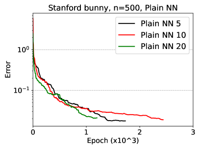
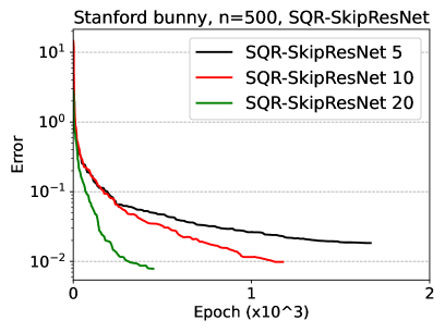
Figure 12: Example 3: Profiles of the validation errors for interpolating the the Stanford bunny for different number of layers using (a) Plain NN and (b) SQR-SkipResNet.

Example 4

In our final example, we delve into the performance evaluation of the proposed SQR-SkipResNet for solving the inverse problem, specifically focusing on the Burgers’ equation. The ground truth coefficients are $\lambda_{1}=1$ and $\lambda_{2}=\nu=\frac{1}{100\pi}=0.003183$, while the initial estimates are $\lambda_{1}=2.0$ and $\lambda_{2}=0.2$. The outcomes of the investigation are presented in Figure 13, which showcases the results obtained during training and validation for $n=500$ using the L-BFGS-B optimizer.

Further analysis is conducted for different network architectures. Figure 13(a) demonstrates the outcomes for the configuration $(n_{l},n_{n})=(10,50)$, revealing improved accuracy for both collocation and validation data when employing the proposed method. The predicted values of $\lambda_{1}$ using SQR-SkipResNet and Plain NN show errors of 0.25% and 0.35%, respectively, when compared with the exact results. Additionally, the percentage errors for predicting $\lambda_{1}$ and $\lambda_{2}$ are 1.55% and 3.29% for SQR-SkipResNet and Plain NN, respectively. Extending this analysis, Fig. 13(b) showcases the results for $(n_{l},n_{n})=(20,50)$. It is evident that a deeper network architecture leads to enhanced accuracy when utilizing the proposed method. Notably, as the number of hidden layers increases, Plain NN demonstrates larger errors. This effect is more pronounced in Fig. 13(c), which presents the results for a large number of hidden layers $(n_{l}=50)$. Consequently, we can conclude that the proposed neural network architecture not only improves accuracy but also exhibits greater stability concerning varying numbers of hidden layers.

Comparing the two plots, we observe that the accuracy difference between Plain NN and SQR-SkipResNet becomes more pronounced as the network size increases. This emphasizes the crucial role of architecture selection in achieving stable results.

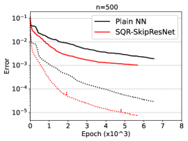
(a) $(n_{l},n_{n})=(10,50)$.

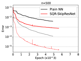
(b) $(n_{l},n_{n})=(20,50)$.

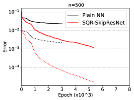
(c) $(n_{l},n_{n})=(50,50)$.

Figure 13: Example 4: Profiles of training (dotted line) and validation error (solid line) for different number of layers.

6 Conclusion

Throughout this study, we conducted a series of experiments to assess how different neural network setups, including Plain NN and SQR-SkipResNet, perform when it comes to interpolating both smooth and complex functions. Our findings consistently showed that SQR-SkipResNet outperforms other architectures in terms of accuracy. This was especially evident when dealing with non-smooth functions, where SQR-SkipResNet displayed improved accuracy, although it might take slightly more time to converge. We also applied our approach to real-world examples, like interpolating the shape of a volcano and the Stanford bunny. In both cases, SQR-SkipResNet exhibited better accuracy, convergence, and computational time compared to Plain NN.

Furthermore, while opting for a deeper network might at times lead to reduced accuracy for both Plain NN and SQR-SkipResNet, we observed that this outcome is influenced by the specific problem. For instance, when dealing with the complicated geometry of the Stanford Bunny and its smooth function, we noticed that deeper networks yielded enhanced accuracy, quicker convergence, and improved CPU efficiency. Regardless of whether deeper networks are suitable, the proposed method demonstrated superior performance. As the effectiveness of network depth varies based on the problem, our approach offers a more favorable architecture choice for networks of different depths.

Additionally, when applied to solve the inverse Burgers’ equation using a physics-informed neural network, our proposed architecture showcased significant accuracy and stability improvements across different numbers of hidden layers, unlike Plain NN. Prospective studies might delve into further optimizations, extensions, and applications of the SQR-SkipResNet framework across diverse domains, particularly for addressing a broad range of inverse problems coupled with PINN methodologies.

References

- [1] Raissi, M., P. Perdikaris, and G.E. Karniadakis, Physics-informed neural networks: A deep learning framework for solving forward and inverse problems involving nonlinear partial differential equations. Journal of Computational Physics, 378: p. 686-707, 2019.
- [2] Kaiming He, Xiangyu Zhang, Shaoqing Ren, and Jian Sun. Deep residual learning for image recognition. arXiv preprint arXiv:1512.03385, 2015.
- [3] Kaiming He, Xiangyu Zhang, Shaoqing Ren, and Jian Sun. Identity mappings in deep residual networks. arXiv preprint arXiv:1603.05027, 2016.
- [4] Hao Li, Zheng Xu, Gavin Taylor, Christoph Studer, Tom Goldstein: Visualizing the Loss Landscape of Neural Nets, arxiv.1712.09913v3, 2018.
- [5] Veit, A., M. Wilber, and S. Belongie, Residual networks behave like ensembles of relatively shallow networks, in Proceedings of the 30th International Conference on Neural Information Processing Systems. Curran Associates Inc.: Barcelona, Spain. p. 550–558, 2016.
- [6] S. Jastrzębski, Arpit D, Ballas N, Verma V, Che T, Bengio Y: Residual Connections Encourage Iterative Inference. arXiv:1710.04773, 2017.
- [7] Lu, Lu., M. Dao, P. Kumar, U. Ramamurty, G.E. Karniadakis, and S. Suresh, Extraction of mechanical properties of materials through deep learning from instrumented indentation. Proceedings of the National Academy of Sciences, 117(13): p. 7052-7062, 2020.
- [8] Wang, S., Y. Teng, and P. Perdikaris, Understanding and Mitigating Gradient Flow Pathologies in Physics-Informed Neural Networks. SIAM Journal on Scientific Computing, 43(5): p. A3055-A3081, 2021.
- [9] R. Franke, Scattered data interpolation: tests of some methods, Mathematics of Computation 38 , 181–200, 1982.
- [10] C.-S. Chen, A. Noorizadegan, C.S. Chen, D.L. Young, On the selection of a better radial basis function and its shape parameter in interpolation problems, Applied Mathematics and Computation 442, 12771, 2023.
- [11] denizunlusu / Getty Images. (n.d.). Mt Eden, or Maungawhau, is a significant Māori site. Retrieved from https://www.lonelyplanet.com/articles/top-things-to-do-in-auckland
- [12] Mira Bozzini, Milvia Rossini. Testing methods for 3d scattered data interpolation. Multivariate Approximation and Interpolation with Applications, 20, 2002.