Abstract

We study the real-valued combinatorial pure exploration of the multi-armed bandit in the fixed-budget setting. We first introduce the Combinatorial Successive Asign (CSA) algorithm, which is the first algorithm that can identify the best action even when the size of the action class is exponentially large with respect to the number of arms. We show that the upper bound of the probability of error of the CSA algorithm matches a lower bound up to a logarithmic factor in the exponent. Then, we introduce another algorithm named the Minimax Combinatorial Successive Accepts and Rejects (Minimax-CombSAR) algorithm for the case where the size of the action class is polynomial, and show that it is optimal, which matches a lower bound. Finally, we experimentally compare the algorithms with previous methods and show that our algorithm performs better.

1 Introduction

The multi-armed bandit (MAB) model is an important framework in online learning since it is useful to investigate the trade-off between exploration and exploitation in decision-making problems (Auer et al.,, 2002; Audibert et al.,, 2009). Although investigating this trade-off is intrinsic in many applications, some application domains only focus on obtaining the optimal object, e.g., an arm or a set of arms, among a set of candidates, and do not care about the loss or rewards that occur during the exploration procedure. This learning problem called the pure exploration (PE) task has received much attention (Bubeck et al.,, 2009; Audibert et al.,, 2010).

One of the important sub-fields among PE of MAB is the combinatorial pure exploration of the MAB (CPE-MAB)(Chen et al.,, 2014; Gabillon et al.,, 2016; Chen et al.,, 2017). In the CPE-MAB, we have a set of $d$ stochastic arms, where the reward of each arm $s\in\{1,\ldots,d\}$ follows an unknown distribution with mean $\mu_{s}$, and an action class $\mathcal{A}$, which is a collection of subsets of arms with certain combinatorial structures. Then, the goal is to identify the best action from the action class $\mathcal{A}$ by pulling a single arm each round. There are mainly two settings in the CPE-MAB. One is the fixed confidence setting, where the player tries to identify the optimal action with high probability with as few rounds as possible, and the other is the fixed-budget setting, where the player tries to identify the optimal action with a fixed number of rounds (Chen et al.,, 2014; Katz-Samuels et al.,, 2020; Wang and Zhu, 2022a, ). Abstractly, the goal is to identify $\boldsymbol{\pi}^{*}$, which is the optimal solution for the following constraint optimization problem:

$$\begin{array}[]{ll@{}ll}\text{maximize}_{\boldsymbol{\pi}}&\boldsymbol{\mu}^{\top}\boldsymbol{\pi}&\\ \text{subject to}&\boldsymbol{\pi}\in\mathcal{A},&\end{array}$$ (1)

where $\boldsymbol{\mu}$ is a vector whose $s$-th element is the mean reward of arm $s$ and $\top$ denotes the transpose.

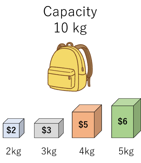
Figure 1: A simple sketch of the knapsack problem. We want to know how many of each item should be included in the bag to maximize the total value. Here, the total weight of every item cannot exceed 10kg, which is the capacity of the bag.

Although CPE-MAB can be applied to many models which can be formulated as (1), most of the existing works in CPE-MAB (Chen et al.,, 2014; Wang and Zhu, 2022b, ; Gabillon et al.,, 2016; Chen et al.,, 2017; Du et al.,, 2021; Chen et al.,, 2016) assume $\mathcal{A}\subseteq\{0,1\}^{d}$. This means that although we can apply the CPE-MAB framework to the shortest path problem (Sniedovich,, 2006), top-$K$ arms identification (Kalyanakrishnan and Stone,, 2010), matching (Gibbons,, 1985), and spanning trees (Pettie and Ramachandran,, 2002), we cannot apply it to problems where $\mathcal{A}\subset\mathbb{R}^{d}$, such as the optimal transport problem (Villani,, 2008), the knapsack problem (Dantzig and Mazur,, 2007), and the production planning problem (Pochet and Wolsey,, 2010). For instance, in the knapsack problem shown in Figure 1, actions are not binary vectors since, for each item, we can put more than one in the bag, e.g., one blue one and two orange ones.

To overcome this limitation, Nakamura and Sugiyama, 2023a introduced the real-valued CPE-MAB (R-CPE-MAB), where the action class is a set of real vectors, i.e., $\mathcal{A}\subset\mathbb{R}^{d}$. Though they have investigated the R-CPE-MAB in the fixed confidence setting, there is still room for investigation in the fixed-budget setting. To the best of our knowledge, the only existing work that can be applied to the fixed-budget R-CPE-MAB is the Peace algorithm introduced by Katz-Samuels et al., (2020). However, there are some issues with the Peace algorithm. Firstly, since the Peace algorithm requires enumerating all the actions in advance, it is impractical when $\mathcal{A}$ is exponentially large in $d$. Secondly, there is a hyper-parameter for it, and one needs to carefully choose them for the feasibility of the Peace algorithm (Yang and Tan,, 2022). Finally, it needs an assumption that the rewards follow a standard normal distribution, which may not be satisfied in real-world applications.

In this work, we first introduce a parameter-free algorithm named the Combinatorial Successive Asign (CSA) algorithm, which is a generalized version of the Combinatorial Successive Accepts and Rejects (CSAR) algorithm proposed by Chen et al.,(2014) for the ordinary CPE-MAB. The CSA algorithm is the first algorithm that can be applied to the fixed-budget R-CPE-MAB even when the size of the action class $\mathcal{A}$ is exponentially large in $d$. We show that the upper bound of the probability of error of the CSA algorithm matches a lower bound up to a logarithmic factor in the exponent.

Since the CSA algorithm does not match a lower bound, we introduce another algorithm named the Minimax Combinatorial Successive Accepts and Rejects (Minimax-CombSAR) algorithm inspired by Yang and Tan, (2022) for the case where the size of the action class is polynomial. In Section 4, we show that the Minimax-CombSAR algorithm is optimal, which means that the upper bound of the probability of error of the best action matches a lower bound. We also show that the Minimax-CombSAR algorithm has only one hyper-parameter, and is easily interpreted.

Finally, we report the results of numerical experiments. First, we show that the CSA algorithm can identify the best action in a knapsack problem, where the size of the action class can be exponentially large in $d$. Then, when the size of the action class is polynomial in $d$, we show that the Minimax-CombSAR algorithm performs better than the CSA algorithm and the Peace algorithm in identifying the best action in a knapsack problem.

2 Problem Formulation

In this section, we formally define our R-CPE-MAB model. Suppose we have $d$ arms, numbered $1,\ldots,d$. Assume that each arm $s\in[d]$ is associated with a reward distribution $\phi_{s}$, where $[d]=\{1,\ldots,d\}$. We assume all reward distributions have $R$-sub-Gaussian tails for some known constant $R>0$. Formally, if $X$ is a random variable drawn from $\phi_{s}$ for some $s\in[d]$, then, for all $\lambda\in\mathbb{R}$, we have $\mathbb{E}[\exp(\lambda X-\lambda\mathbb{E}[X])]\leq\exp(R^{2}\lambda^{2}/2)$. It is known that the family of $R$-sub-Gaussian tail distributions includes all distributions that are supported on $[a,b]$, where $(b-a)/2=R$, and also many unbounded distributions such as Gaussian distributions with variance $R^{2}$ (Rivasplata,, 2012; Rinaldo and Bong,, 2018). Let $\boldsymbol{\mu}=(\mu_{1},\ldots,\mu_{d})^{\top}$ denote the vector of expected rewards, where each element $\mu_{s}=\mathbb{E}_{X\sim\phi_{s}}[X]$ denotes the expected reward of arm $s$ and $\top$ denotes the transpose. With a given $\boldsymbol{\nu}$, let us consider the following linear optimization problem:

$$\begin{array}[]{ll@{}ll}\text{maximize}_{\boldsymbol{\pi}}&\boldsymbol{\nu}^{\top}\boldsymbol{\pi}&\\ \text{subject to}&\boldsymbol{\pi}\in\mathcal{C}\subset\mathbb{R}_{\geq 0}^{d}.&\end{array}$$ (2)

Here, $\mathcal{C}$ is a problem-dependent feasible region of $\boldsymbol{\pi}$, which satisfies some combinatorial structures. Then, for any $\boldsymbol{\nu}\in\mathbb{R}^{d}$, we denote by $\boldsymbol{\pi}^{\boldsymbol{\nu},\mathcal{C}}$ the solution of (2). We define the action class $\mathcal{A}$ as the set of vectors that contains optimal solutions of (2) for any $\boldsymbol{\nu}$, i.e.,

$$\mathcal{A}=\left\{\boldsymbol{\pi}^{\boldsymbol{\nu,\mathcal{C}}}\in\mathbb{R}_{\geq 0}^{d}\ |\ \forall\boldsymbol{\nu}\in\mathbb{R}^{d}\right\}.$$ (3)

We assume that the size of $\mathcal{A}$ is finite and denote it by $K$. This assumption is relatively mild since, for instance, in linear programming, the optimal solution can always be found at one of the vertices of the feasible region (Ahmadi,, 2016).

Also, let $\texttt{POSSIBLE-PI}(s)=\{x\in\mathbb{R}\ |\ \exists\boldsymbol{\pi}\in\mathcal{A},\pi_{s}=x\}$, where $\pi_{s}$ denote the $s$-th element of $\boldsymbol{\pi}$. We can see POSSIBLE-PI($s$) as the set of all possible values that an action in the action set can take as the $s$-th element. Let us denote the size of $\texttt{POSSIBLE-PI}(s)$ by $B_{s}$. Note that $K$, the size of $\mathcal{A}$, can be exponentially large in $d$, i.e., $|\mathcal{A}|=\mathcal{O}(\prod_{s=1}^{d}B_{s})$.

We assume we have offline oracles which efficiently solve the linear optimization problem (2) once $\nu$ is given. For instance, algorithms which output $\boldsymbol{\pi}^{*}({\boldsymbol{\nu}})~{}=~{}\mathop{\rm arg~{}max}\limits_{\boldsymbol{\pi}\in\mathcal{A}}\boldsymbol{\nu}^{\top}\boldsymbol{\pi}$ in polynomial or pseudo-polynomial time in $d$.

The player’s objective is to identify the best action $\boldsymbol{\pi}^{*}=\mathop{\rm arg~{}max}\limits_{\boldsymbol{\pi}\in\mathcal{A}}\boldsymbol{\mu}^{\top}\boldsymbol{\pi}$ by pulling a single arm each round. The player is given a budget $T$, and cannot pull arms more than $T$ times. The player outputs an action $\boldsymbol{\pi}^{\mathrm{out}}$ at the end, and she is evaluated by the probability of error, which is formally $\Pr\left[\boldsymbol{\pi}^{\mathrm{out}}\neq\boldsymbol{\pi}^{*}\right]$.

3 Lower Bound of the Fixed-Budget R-CPE-MAB

In this section, we show a lower bound of the probability of error in R-CPE-MAB. As preliminaries, let us introduce some notions. First, we introduce $\boldsymbol{\pi}^{(s)}$ as follows (Nakamura and Sugiyama, 2023b, ):

$$\boldsymbol{\pi}^{(s)}=\mathop{\rm arg~{}min}\limits_{\boldsymbol{\pi}\in\mathcal{A}\setminus\left\{\boldsymbol{\pi}^{*}\right\}}\frac{\boldsymbol{\mu}^{\top}\left(\boldsymbol{\pi}^{*}-\boldsymbol{\pi}\right)}{\left|\pi^{*}_{s}-\pi_{s}\right|}.$$ (4)

Intuitively, among the actions whose $s$-th element is different from $\boldsymbol{\pi}^{*}$, $\boldsymbol{\pi}^{(s)}$ is the action which is the most difficult to determine whether it is the best action or not. We also introduce the notion G-gap (Nakamura and Sugiyama, 2023b, ) as follows:

$$\Delta_{s} = \min_{{\boldsymbol{\pi}\in\mathcal{A}\setminus\left\{\boldsymbol{\pi}^{*}\right\}}}\frac{\boldsymbol{\mu}^{\top}\left(\boldsymbol{\pi}^{*}-\boldsymbol{\pi}\right)}{\left|\pi^{*}_{s}-\pi_{s}\right|}$$ (5)

$$= \frac{\boldsymbol{\mu}^{\top}\left(\boldsymbol{\pi}^{*}-\boldsymbol{\pi}^{(s)}\right)}{\left|\pi_{s}^{*}-\pi^{(s)}_{s}\right|}.$$

G-Gap was first introduced in Nakamura and Sugiyama, 2023b as a natural generalization of the notion gap in the CPE-MAB literature (Chen et al.,, 2014, 2016, 2017). This was introduced as a key notion that characterizes the difficulty of the problem instance.

In Theorem 1, we show that the sum of the inverse of squared G-Gaps,

$$\mathbf{H}=\sum_{s=1}^{d}\left(\frac{1}{\Delta_{s}}\right)^{2},$$ (6)

appears in the lower bound of the probability of error of R-CPE-MAB, which implies that it characterizes the difficulty of the problem instance.

Theorem 1.

For any action class and any algorithm that returns an action $\boldsymbol{\pi}^{\mathrm{out}}$ after $T$ times of arm pulls, the probability of error is at least

$$\mathcal{O}\left(\exp\left(-\frac{T}{\mathbf{H}}\right)\right).$$ (7)

We show the proof in Appendix A. If $\mathcal{A}$ is a set of $d$ dimensional standard basis, R-CPE-MAB becomes the standard best arm identification problem whose objective is to identify the best arm with the largest expected reward among $d$ arms (Bubeck et al.,, 2009; Audibert et al.,, 2010; Carpentier and Locatelli,, 2016). From Carpentier and Locatelli, (2016), a lower bound is $\mathcal{O}\left(\exp\left(-\frac{T}{\log(d)\mathbf{H}}\right)\right)$ for the standard best arm identification problem. It is a future work that whether the lower bound is $\mathcal{O}\left(\exp\left(-\frac{T}{\log(d)\mathbf{H}}\right)\right)$ for general action classes.

4 The Combinatorial Successive Assign (CSA) Algorithm

In this section, we first introduce the CSA algorithm, which can be seen as a generalization of the CSAR algorithm (Chen et al.,, 2014). This algorithm can be applied to fixed-budget R-CPE-MAB even when the size of the action class $\mathcal{A}$ is exponentially large in $d$. Then, we show an upper bound of the probability of error of the best action of the CSA algorithm. We also discuss the number of times offline oracles have to be called.

4.1 CSA Algorithm

In this subsection, we introduce the CSA algorithm, a fully parameter-free algorithm for fixed-budget R-CPE-MAB that works even when the action set $\mathcal{A}$ can be exponentially large in $d$.

We first define the constrained offline oracle which is used in the CSA algorithm.

Definition 1 (Constrained offline oracle).

Let $\boldsymbol{S}=\{(e,x)|(e,x)\in\mathbb{Z}\times\mathbb{R}\}$ be a set of tuples. A constrained offline oracle is denoted by $\mathrm{COracle}$: $\mathbb{R}^{d}\times\boldsymbol{S}\rightarrow\mathcal{A}\ \cup\perp$ and satisfies

$$\mathrm{COracle}(\boldsymbol{\mu},\boldsymbol{S})=\left\{\begin{array}[]{ll}\mathop{\rm arg~{}max}\limits_{\boldsymbol{\pi}\in\mathcal{A}_{\boldsymbol{S}}}\boldsymbol{\mu}^{\top}\boldsymbol{\pi}&(\mathrm{if}\ \mathcal{A}_{\boldsymbol{S}}\neq\emptyset),\\ \perp&(\mathrm{if}\ \mathcal{A}_{\boldsymbol{S}}=\emptyset),\\ \end{array}\right.$$

where we define $\mathcal{A}_{\boldsymbol{S}}=\left\{\boldsymbol{\pi}\in\mathcal{A}\ |\ \forall(e,x)\in\boldsymbol{S},\pi_{e}=x\right\}$ as the collection of feasible actions and $\perp$ is a null symbol.

Here, we can see that a COracle is a modification of an offline oracle specified by $\boldsymbol{S}$. In other words, for all $(e,x)$ in $\boldsymbol{S}$, the COracle outputs an action whose $e$-th element is $x$; otherwise, it outputs the null symbol. In Appendix B, we discuss how to construct such COracles for some combinatorial problems, such as the optimal transport problem and the knapsack problem.

We introduce the CSA algorithm in Algorithm 1. The CSA algorithm divides the budget into $d$ rounds. In each round, we pull each of the remaining arms the same number of times (line 5). At each round $t$, the CSA outputs the empirically best action $\hat{\boldsymbol{\pi}}(t)$ (line 6), chooses a single arm $p(t)$ (line 14), and assigns $\hat{\pi}_{p(t)}(t)$ for the $e$-th element of $\boldsymbol{\pi}^{\mathrm{out}}$. Indices that are assigned are maintained in $\boldsymbol{F}(t)$, and arms $s\in F(t)$ will no longer be pulled in the next rounds. The pair of the index and the assigned value for $\boldsymbol{\pi}^{\mathrm{out}}$, $\boldsymbol{S}(t)$, is updated at every round (line 16).

Algorithm 1 CSA: Combinatorial Successive Assign Algorithm

0:  Budget: $T\geq 0$; COracle: $\rightarrow\mathcal{A}\cup\{\perp\}$

1:  Define $\tilde{\log}(n)=\sum_{i=1}^{d}\frac{1}{i}$

2:  $\tilde{T}_{0}\leftarrow 0$, $\boldsymbol{F}(t)\leftarrow\emptyset$, $\boldsymbol{S}(t)=\emptyset$

3:  for $t=1\ \mathrm{to}\ d$ do

4:     $\tilde{T}(t)\leftarrow\lceil\frac{T-d}{\tilde{\log}(d)(d-t+1)}\rceil$

5:     Pull each arm $e\in[d]\setminus F(t)$ for $\tilde{T}(t)-\tilde{T}_{t-1}$ times

6:     $\hat{\boldsymbol{\pi}}(t)\leftarrow\mathrm{COracle}(\hat{\boldsymbol{\mu}}(t),\boldsymbol{S}(t))$

7:     if $\hat{\boldsymbol{\pi}}(t)=\perp$ then

8:        Fail: set ${\boldsymbol{\pi}}^{\mathrm{out}}\leftarrow\perp$ and return ${\boldsymbol{\pi}}^{\mathrm{out}}$

9:     end if

10:     for all  $e$ in $[d]\setminus\boldsymbol{F}(t)$ do

11:        $\texttt{CHECK(e)}\leftarrow\texttt{POSSIBLE-PI(e)}\setminus\left\{\hat{\pi}_{e}(t)\right\}$

12:        $\tilde{\boldsymbol{\pi}}^{e}(t)\leftarrow\mathop{\rm arg~{}max}\limits_{x\in\texttt{CHECK(e)}}\mathrm{COracle}(\hat{\boldsymbol{\mu}}(t),\boldsymbol{S}(t)\cup(e,x))$

13:     end for

14:     $p(t)\leftarrow\mathop{\rm arg~{}max}\limits_{e\in[d]\setminus F(t)}\frac{\langle\hat{\boldsymbol{\mu}}(t),\hat{\boldsymbol{\pi}}(t)-\tilde{\boldsymbol{\pi}}^{e}(t)\rangle}{\hat{\pi}_{e}(t)-\tilde{\pi}^{e}_{e}(t)}$

15:     $\boldsymbol{F}(t+1)\leftarrow\boldsymbol{F}(t)\cup\{p(t)\}$

16:     $\boldsymbol{S}(t+1)\leftarrow\boldsymbol{S}(t)\cup\{(p(t),\hat{\pi}_{p(t)}(t)\}$

17:  end for

18:  // Convert $\boldsymbol{S}(d+1)$ to $\boldsymbol{\pi}^{\mathrm{out}}$

19:  for $(e,x)\ \mathrm{in}\ \boldsymbol{S}(d+1)$ do

20:     // The $e$-th element of $\boldsymbol{\pi}^{\mathrm{out}}$ is $x$

21:     $\pi^{\mathrm{out}}_{e}=x$

22:  end for

23:  return  ${\boldsymbol{\pi}}^{\mathrm{out}}$

4.2 Theoretical Analysis of CSA Algorithm

Here, we first discuss an upper bound of the probability of error. Then, we discuss the number of times we call the offline oracle.

4.2.1 An Upper Bound of the Probability of Error

Here, we show an upper bound of the probability of error of the CSA algorithm. Let $\Delta_{(1)},\ldots,\Delta_{(d)}$ be a permutation of $\Delta_{1},\ldots,\Delta_{d}$ such that $\Delta_{(1)}\leq\cdots\leq\Delta_{(d)}$. Also, let us define

$$\mathbf{H}_{2}=\max_{s\in[d]}\frac{s}{\Delta^{2}_{(s)}}.$$

One can verify that $\mathbf{H}_{2}$ is equivalent to $\mathbf{H}$ up to a logarithmic factor: $\mathbf{H}_{2}\leq\mathbf{H}\leq\log(2d)\mathbf{H}_{2}$ (Audibert et al.,, 2010).

Theorem 2.

Given any $T>d$, action class $\mathcal{A}\subset\mathbb{R}^{d}$, and $\boldsymbol{\mu}\in\mathbb{R}^{d}$, the CSA algorithm uses at most $T$ samples and outputs a solution $\boldsymbol{\pi}^{\mathrm{out}}\in\mathcal{A}\cup\{\perp\}$ such that

$$\Pr\left[\boldsymbol{\pi}^{\mathrm{out}}\neq\boldsymbol{\pi}^{*}\right]$$ (8)

$$\leq d^{2}\exp\left(-\frac{T-d}{2(2+L^{2})^{2}R^{2}\tilde{\log}(d)U_{\mathcal{A}}^{2}\mathbf{H}_{2}}\right),$$

where $L=\max_{e\in[d],\boldsymbol{\pi}^{1},\boldsymbol{\pi}^{2},\boldsymbol{\pi}^{3}\in\mathcal{A},\pi^{1}_{e}\neq\pi^{3}_{e}}\frac{\left|\pi^{1}_{e}-\pi^{2}_{e}\right|}{\left|\pi^{1}_{e}-\pi^{3}_{e}\right|}$, $\tilde{\log}(d)\triangleq\sum_{s=1}^{d}\frac{1}{s}$, and $U_{\mathcal{A}}=\max_{\boldsymbol{\pi},\boldsymbol{\pi}^{\prime}\in\mathcal{A},e\in\{s\in[d]\ |\ \pi_{s}\neq\pi^{\prime}_{s}\}}\frac{\sum_{s=1}^{d}|\pi_{s}-\pi^{\prime}_{s}|}{|\pi_{e}-\pi^{\prime}_{e}|}$.

We can see that the CSA algorithm is optimal up to a logarithmic factor in the exponent. Since $L=1$ and $U_{\mathcal{A}}=\mathrm{width}(\mathcal{A})$ in the ordinary CPE-MAB, we can confirm that Theorem 2 can be seen as a natural generalization of Theorem 3 in Chen et al., (2014), which shows an upper bound of the probability of error of the CSAR algorithm.

4.2.2 The Oracle Complexity

Next, we discuss the oracle complexity, the number of times we call the offline oracle (Ito et al.,, 2019; Xu and Li,, 2021). Note that, in the CSA algorithm, we call the COracle $\mathcal{O}(d\sum_{s=1}^{d}B_{s})$ times (line 12). Therefore, if each COracle call invokes the offline oracle $N$ times, the oracle complexity is $\mathcal{O}\left(Nd\sum_{s=1}^{d}B_{s}\right)$. Finally, if the time complexity of each oracle call is $Z$, then the total time complexity of the CSA algorithm is $\mathcal{O}\left(ZNd\sum_{s=1}^{d}B_{s}\right)$.

Below, we discuss the oracle complexity of the CSA algorithm in some specific combinatorial problems such as the knapsack problem and the optimal transport problem. Note that the Minimax-CombSAR algorithm and Peace algorithm Katz-Samuels et al., (2020) have to enumerate all the actions in advance, where the number may be exponentially large in $d$. We show that the CSA algorithm mitigates the curse of dimensionality.

The Knapsack Problem (Dantzig and Mazur,, 2007). In the knapsack problem, we have $d$ items. Each item $s\in[d]$ has a weight $w_{s}$ and value $v_{s}$. Also, there is a knapsack whose capacity is $W$ in which we put items. Our goal is to maximize the total value of the knapsack, not letting the total weight of the items exceed the capacity of the knapsack. Formally, the optimization problem is given as follows:

$$\begin{array}[]{ll@{}ll}\text{maximize}_{\boldsymbol{\boldsymbol{\pi}}\in\mathcal{A}}&\sum_{s=1}^{d}v_{s}\pi_{s}&\\ \\ \text{subject to}&\sum_{s=1}^{d}\pi_{s}w_{s}\leq W,&\end{array}$$

where $\pi_{s}\in\mathbb{Z}_{\geq 0}$ denotes the number of item $s$ in the knapsack. Here, if we assume the weight of each item is known, but the value is unknown, we can apply the R-CPE-MAB framework to the knapsack problem, where we estimate the values of items. The knapsack problem is NP-complete (Garey and Johnson,, 1979). Hence, it is unlikely that the knapsack problem can be solved in polynomial time. However, it is well known that the knapsack problem can be solved in pseudo-polynomial time $\mathcal{O}(dW)$ if we use dynamic programming (Kellerer et al.,, 2004; Fujimoto,, 2016). It finds the optimal solution by constructing a table of size $dW$ whose $(s,w)$-th element represents the maximum total value that can be achieved if the sum of the weights does not exceed $w$ using up to the $s$th item. In some cases, it is sufficient to assume $\mathcal{O}(dW)$ time-complexity is enough, and therefore, we use this dynamic programming method as the offline oracle. We can construct the COrcale for the knapsack problem by calling this offline oracle once (see Appendix B.1 for details). Therefore, the CSA algorithm calls the offline oracle $\mathcal{O}(1\times d\sum_{s=1}^{d}B_{s})=\mathcal{O}(d\sum_{s=1}^{d}B_{s})$ times, and the total time complexity of the CSA algorithm is $\mathcal{O}(dW\times d\sum_{s=1}^{d}B_{s})=\mathcal{O}(d^{2}\sum_{s=1}^{d}B_{s}W)$. This is much more computationally friendly than the Peace algorithm with time complexity $\mathcal{O}\left(\prod_{s=1}^{d}B_{s}\right)$.

The Optimal Transport (OT) Problem (Peyré and Cuturi,, 2019). OT can be regarded as the cheapest plan to deliver resources from $m$ suppliers to $n$ consumers, where each supplier $i$ and consumer $j$ have supply $s_{i}$ and demand $d_{j}$, respectively. Let $\boldsymbol{\gamma}\in\mathbb{R}^{m\times n}_{\geq 0}$ be the cost matrix, where $\gamma_{ij}$ denotes the cost between supplier $i$ and demander $j$. Our objective is to find the optimal transportation matrix

$$\boldsymbol{\pi}^{*}=\mathop{\rm arg~{}min}\limits_{\boldsymbol{\pi}\in\mathcal{G}(\boldsymbol{s},\boldsymbol{d})}\sum_{i,j}\pi_{ij}\gamma_{ij},$$ (9)

where

$$\mathcal{G}(\boldsymbol{s},\boldsymbol{d})\triangleq\left\{\boldsymbol{\Pi}\in\mathbb{R}^{m\times n}_{\geq 0}\,\middle|\,\boldsymbol{\Pi}\boldsymbol{1}_{n}=\boldsymbol{s},\boldsymbol{\Pi}^{\top}\boldsymbol{1}_{m}=\boldsymbol{d}\right\}.$$ (10)

Here, $\boldsymbol{s}=(s_{1},\ldots,s_{m})$ and $\boldsymbol{d}=(d_{1},\ldots,d_{n})$. $\pi_{ij}$ represents how much resources one sends from supplier $i$ to demander $j$. Here, if we assume that the cost is unknown and changes stochastically, e.g., due to some traffic congestions, we can apply the R-CPE-MAB framework to the optimal transport problem, where we estimate the cost of each edge $\left(i,j\right)$ between supplier $i$ and consumer $j$.

Once $\boldsymbol{\gamma}$ is given, we can compute $\boldsymbol{\pi}^{*}$ in $\mathcal{O}(l^{3}\log l)$, where $l=\max\left(m,n\right)$, by using network simplex or interior point methods (Cuturi,, 2013), and we can use them as the offline oracle. It is known that the solution of linear programming can always be found at one of the vertices of the feasible region (Ahmadi,, 2016), and therefore the size of the action space $\mathcal{A}=\left\{\boldsymbol{\pi}^{\boldsymbol{\nu,\mathcal{G}(\boldsymbol{s},\boldsymbol{d})}}\in\mathbb{R}_{\geq 0}^{m\times n}\ |\ \forall\boldsymbol{\nu}\in\mathbb{R}^{m\times n}\right\}$ is finite. However, it is difficult to construct $\left\{\texttt{POSSIBLE-PI}\left(\left(i,j\right)\right)\right\}_{i\in[m],j\in[n]}$ in general to run the CSA algorithm. On the other hand, if $\boldsymbol{s}$ and $\boldsymbol{d}$ are both integer vectors, we can construct $\left\{\texttt{POSSIBLE-PI}\left(\left(i,j\right)\right)\right\}_{i\in[m],j\in[n]}$ thanks to the fact that $\mathcal{A}=\left\{\boldsymbol{\pi}^{\boldsymbol{\nu,\mathcal{G}(\boldsymbol{s},\boldsymbol{d})}}\in\mathbb{Z}_{\geq 0}^{m\times n}\ |\ \forall\boldsymbol{\nu}\in\mathbb{R}^{m\times n}\right\}$ is a set of non-negative integer matrices (Goodman and O’Rourke,, 1997). In this case, all actions are restricted to non-negative integers, and $\texttt{POSSIBLE-PI}(i,j)=\left\{0,1,\ldots,\min\left(s_{i},d_{j}\right)\right\}$. In Appendix B.2, we show that the COracle can be constructed by calling the offline oracle once. Therefore, we call the offline oracle $\mathcal{O}\left(1\times mn\sum_{s=1}^{mn}B_{s}\right)=\mathcal{O}(mn\sum_{s=1}^{mn}B_{s})$ times, and the total time complexity is $\mathcal{O}\left(l^{3}\log lmn\sum_{s=1}^{mn}B_{s}\right)$, where $l=\max\left(m,n\right)$. Again, this is much more computationally friendly than the Peace algorithm with time complexity $\mathcal{O}\left(\prod_{s=1}^{d}B_{d}\right)$.

A General Case When $K(=|\mathcal{A}|)=\mathrm{poly}(d).$ In some cases, we can enumerate all the possible actions in $\mathcal{A}$. For instance, one may use some prior knowledge of each arm, which is sometimes obtainable in the real world, to narrow down the list of actions, and make the size of the action class $\mathcal{A}$ polynomial in $d$. In Appendix B.3, we show that the time complexity of the COracle is $\mathcal{O}\left(dK+K\log K\right)$, and therefore the total time complexity of the CSA algorithm is $\mathcal{O}\left((dK+K\log K)\cdot d\sum_{s=1}^{d}B_{s}\right)$.

5 The Minimax-CombSAR Algorithm for R-CPE-MAB where $|\mathcal{A}|=\mathrm{poly}(d)$

In this section, we show an algorithm for fixed-budget R-CPE-MAB named the Minimax Combinatorial Successive Accept (Minimax-CombSAR) algorithm, for the case where we can assume that the size of $\mathcal{A}$ is polynomial in $d$. Let $\mathcal{A}~{}=~{}\{\boldsymbol{\pi}^{1}~{}=~{}\boldsymbol{\pi}^{*},\boldsymbol{\pi}^{2},\ldots,\boldsymbol{\pi}^{K}\}$, where $\boldsymbol{\mu}^{\top}\boldsymbol{\pi}^{i}\geq\boldsymbol{\mu}^{\top}\boldsymbol{\pi}^{i+1}$, for all $i\in[K-1]$. The Minimax-CombSAR algorithm is inspired by the Optimal Design-based Linear Best Arm Identification (OD-LinBAI) algorithm Yang and Tan, (2022), which eliminates actions in order from those considered suboptimal and finally outputs the remaining action as the optimal action. For the Minimax-CombSAR algorithm, we show an upper bound of the probability of error.

5.1 Minimax-CombSAR Algorithm

We show the Minimax-CombSAR in Algorithm 2. Here, we explain it at a higher level.

We have $\lceil\log d\rceil$ phases in the Minimax-CombSAR algorithm, and it maintains an active action set $\mathbb{A}(r)$ in each phase $r$. In each phase $r\in[\lceil\log d\rceil]$, it pulls arms $m(r)=\frac{T^{\prime}-d\lceil\log_{2}d\rceil}{B/2^{r-1}}$ times in total, where $B=2^{\left\lceil\log_{2}d\right\rceil}-1$ and $\beta\in[0,1]$ is a hyperparameter, and $T^{\prime}=T-\left\lfloor\frac{T}{d}\beta\right\rfloor\times d$. In each phase, we compute an allocation vector $\boldsymbol{p}(r)\in\left\{\boldsymbol{v}\in\mathbb{R}^{d}\ |\ \sum_{s=1}^{d}v_{s}=1\right\}\triangleq\Pi_{d}$, and pull each arm $s$ $\lceil p_{s}(r)\cdot m(r)\rceil$ times. Then, at the end of each phase $r$, it eliminates a subset of possibly suboptimal actions. Eventually, there is only one action $\boldsymbol{\pi}^{\mathrm{out}}$ in the active action set, which is the output of the algorithm.

The key to identifying the best action with high confidence is the choice of the allocation vector $\boldsymbol{p}(r)$, which determines how many times we pull each arm in phase $r$.

Algorithm 2 Minimax Combinatorial Successive Accept Algorithm

0:  Budget: $T\geq 0$, initialization parameter: $\beta$, action set: $\mathbb{A}(1)=\mathcal{A}$

1:  // Initialization

2:  for $s\in[d]$ do

3:     Pull arm $s$ $\left\lfloor\frac{T}{d}\beta\right\rfloor$ times and update $\hat{\mu}_{s}(1)$

4:     $T_{s}(r)\leftarrow\left\lfloor\frac{T}{d}\beta\right\rfloor$

5:  end for

6:  $T^{\prime}\leftarrow T-\left\lfloor\frac{T}{d}\beta\right\rfloor\times d$

7:  for $r=1\ \mathrm{to}\ \lceil\log_{2}d\rceil$ do

8:     $m(r)=\frac{T^{\prime}-d\lceil\log_{2}d\rceil}{B/2^{r-1}}$

9:     Compute $\boldsymbol{p}(r)$ according to (13) or (15)

10:     for $s\in[d]$ do

11:        Pull arm $s$ $\left\lceil p_{s}(r)\cdot m(r)\right\rceil$ times

12:        Update $\hat{\mu}_{s}(r+1)$ with the observed samples

13:     end for

14:     For each action $\boldsymbol{\pi}\in\mathbb{A}(r)$, estimate the expected reward: $\langle\hat{\boldsymbol{\mu}}(r+1),\boldsymbol{\pi}\rangle$

15:     Let $\mathbb{A}(r+1)$ be the set of $\left\lceil\frac{d}{2^{r}}\right\rceil$ actions in $\mathbb{A}(r)$ with the largest estimates of the expected rewards

16:  end for

16:  The only action $\boldsymbol{\pi}^{\mathrm{out}}$ in $\mathbb{A}(\lceil\log_{2}d\rceil+1)$

Choice of $\boldsymbol{p}(r)$

We discuss how to choose an allocation vector that is beneficial to identify the best action. Let us denote the number of times arm $s$ is pulled before phase $r$ starts by $T_{s}(r)$. Also, we denote by $\hat{\mu}_{s}(r)$ the empirical mean of the reward from arm $s$ before phase $r$ starts. Then, at the end of phase $r$, from Hoeffding’s inequality (Hoeffding,, 1963), we have

$$\Pr\left[\left|(\hat{\boldsymbol{\mu}}(r+1)-\boldsymbol{\mu})^{\top}(\boldsymbol{\pi}^{a}-\boldsymbol{\pi}^{b})\right|\geq\epsilon\right]$$ (11)

$$\leq \exp\left(-\frac{\epsilon^{2}}{\kappa^{a,b,\boldsymbol{p}}(r)R^{2}}\right)$$

for any $\boldsymbol{\pi}^{a},\boldsymbol{\pi}^{b}\in\mathcal{A}$, and $\epsilon\in\mathbb{R}$. Here, $\hat{\boldsymbol{\mu}}(r+1)=(\hat{\mu}_{1}(r+1),\ldots,\hat{\mu}_{d}(r+1))^{\top}$ and

$$\kappa^{a,b,\boldsymbol{p}}(r)=\sum_{s=1}^{d}\frac{\left(\pi^{a}_{s}-\pi^{b}_{s}\right)^{2}}{T_{s}(r)+\lceil p_{s}(r)\cdot m(r)\rceil}.$$ (12)

(11) shows that the empirical difference $\hat{\boldsymbol{\mu}}^{\top}(\boldsymbol{\pi}^{a}-\boldsymbol{\pi}^{b})$ between $\boldsymbol{\pi}^{a}$ and $\boldsymbol{\pi}^{b}$ is closer to the true difference ${\boldsymbol{\mu}}^{\top}(\boldsymbol{\pi}^{a}-\boldsymbol{\pi}^{b})$ with high probability if we make $\kappa^{a,b,\boldsymbol{p}}(r)$ small. In that case, we have a higher chance to distinguish whether $\boldsymbol{\pi}^{a}$ is better than $\boldsymbol{\pi}^{b}$ or not. However, when we have more than two actions in $\mathbb{A}(r)$,

$$\boldsymbol{p}^{a,b}(r)=\mathop{\rm arg~{}min}\limits_{\boldsymbol{p}\in\Pi_{d}}\kappa^{a,b,\boldsymbol{p}}(r)$$

is not necessarily a good allocation vector for investigating the true difference between other pairs of actions in $\mathbb{A}(r)$. Therefore, we propose the following allocation vector as an alternative:

$$\boldsymbol{p}^{\mathrm{min}}(r)\triangleq\mathop{\rm arg~{}min}\limits_{\boldsymbol{p}\in\Pi_{d}}\max_{\boldsymbol{\pi}^{a},\boldsymbol{\pi}^{b}\in\mathcal{A}}\kappa^{a,b,\boldsymbol{p}}(r).$$ (13)

(13) takes a minimax approach, which computes an allocation vector that minimizes the maximum value of the right-hand side of (11) among all of the pairs of actions in $\mathbb{A}(r)$. Since (13) is a $d$-dimensional non-linear optimization problem, it becomes computationally costly as $d$ grows. Thus, another possible choice of the allocation vector is as follows:

$$\boldsymbol{q}^{\mathrm{min}}(r) \triangleq \mathop{\rm arg~{}min}\limits_{\boldsymbol{p}\in\Pi_{d}}\max_{\boldsymbol{\pi}^{a},\boldsymbol{\pi}^{b}\in\mathcal{A}}\lambda^{a,b,\boldsymbol{p}}(r),$$ (14)

where $\lambda^{a,b,\boldsymbol{p}}=\sum_{s=1}^{d}\frac{\left(\pi^{a}_{s}-\pi^{b}_{s}\right)^{2}}{p_{s}(r)\cdot m(r)}$. For specific actions $\boldsymbol{\pi}^{k},\boldsymbol{\pi}^{l}\in\mathcal{A}$, from the method of Lagrange multipliers (Hoffmann and Bradley,, 2009), we have

$$\boldsymbol{q}^{k,l}(r) \triangleq \mathop{\rm arg~{}min}\limits_{\boldsymbol{p}\in\Pi_{d}}\lambda^{k,l,\boldsymbol{p}}(r)$$

$$= \left(\frac{\left|\pi^{k}_{1}-\pi^{l}_{1}\right|}{\sum_{s=1}^{d}\left|\pi^{k}_{s}-\pi^{l}_{s}\right|},\ldots,\frac{\left|\pi^{k}_{d}-\pi^{l}_{d}\right|}{\sum_{s=1}^{d}\left|\pi^{k}_{s}-\pi^{l}_{s}\right|}\right)^{\top},$$

and therefore, $\boldsymbol{q}^{\mathrm{min}}(r)$ in (14) can be written explicitly as follows:

$$\boldsymbol{q}^{\mathrm{min}}(r) =\boldsymbol{q}^{i,j}(r)$$

$$=\left(\frac{\left|\pi^{i}_{1}-\pi^{j}_{1}\right|}{\sum_{s=1}^{d}\left|\pi^{i}_{s}-\pi^{j}_{s}\right|},\ldots,\frac{\left|\pi^{i}_{d}-\pi^{j}_{d}\right|}{\sum_{s=1}^{d}\left|\pi^{i}_{s}-\pi^{j}_{s}\right|}\right)^{\top},$$ (15)

where $\boldsymbol{\pi}^{i},\boldsymbol{\pi}^{j}=\mathop{\rm arg~{}max}\limits_{\boldsymbol{\pi}^{k},\boldsymbol{\pi}^{l}\in\mathcal{A}}\lambda^{k,l,\boldsymbol{p}}(r)$. If we use (15) for the allocation vector instead of computing (13), we do not have to solve a $d$-dimensional non-linear optimization problem, and thus is computationally more friendly.

In some cases, actions in $\mathcal{A}$ can be sparse, and $\boldsymbol{p}(1)$ can also be sparse. If $\boldsymbol{p}(1)$ is sparse, we may only have a few samples for some arms, and therefore accidentally eliminate the best action in the first phase in line 15 of Algorithm 2. To cope with this problem, we have the initialization phase (lines 2–5) to pull each arm $\left\lfloor\frac{T}{d}\beta\right\rfloor$ times, where $\beta\in[0,1]$ is a hyperparameter. Intuitively, $\beta$ represents how much of the total budget will be spent on the initialization phase. If $\beta$ is too small, we may accidentally eliminate the best action in the early phase, and if it is too large, we may not have enough budget to distinguish between the best action and the next best action.

5.2 Theoretical Analysis of Minimax-CombSAR

Here, in Theorem 3, we show an upper bound of the probability of error of the Minimax-CombSAR algorithm.

Theorem 3.

For any problem instance in fixed-budget R-CPE-MAB, the Minimax-CombSAR algorithm outputs an action $\boldsymbol{\pi}^{\mathrm{out}}$ satisfying

$$\Pr\left[\boldsymbol{\pi}^{\mathrm{out}}\neq\boldsymbol{\pi}^{*}\right]$$

$$\leq\left(\frac{4K}{d}+3\log_{2}d\right)\exp\left(-\frac{T^{\prime}-\left\lceil\log_{2}d\right\rceil}{R^{2}V^{2}}\cdot\frac{1}{\mathbf{H}_{2}}\right),$$ (16)

where $V=\max_{\boldsymbol{\pi}^{i}\in\mathcal{A}\setminus\{\boldsymbol{\pi}^{*}\}}\left(\sum\limits_{s=1}^{d}\frac{\left|\pi^{1}_{s}-\pi^{i}_{s}\right|}{\left|\pi^{1}_{s(i)}-\pi^{i}_{s(i)}\right|}\right)^{2}$ and $s(i)=\mathop{\rm arg~{}max}\limits_{s\in[d]}\left|\pi^{1}_{s}-\pi^{i}_{s}\right|$.

We can see that the Minimax-CombSAR algorithm is an optimal algorithm whose upper bound of the probability of error matches the lower bound shown in (7) since we have $\mathbf{H}_{2}\leq\mathbf{H}\leq\log(2d)\mathbf{H}_{2}$.

5.3 Comparison with Katz-Samuels et al., (2020)

Here, we compare the Minimax-CombSAR algorithm with the Peace algorithm introduced in Katz-Samuels et al., (2020). The upper bound of the Peace algorithm can be written as follows:

$$\Pr\left[\boldsymbol{\pi}^{\mathrm{out}}\neq\boldsymbol{\pi}^{*}\right]$$ (17)

$$\leq 2\left\lceil\log\left(d\right)\right\rceil\exp\left(-\frac{T}{c^{\prime}\log(d)\left(\gamma_{*}+\rho_{*}\right)}\right),$$

where

$$\gamma_{*}=\inf_{\boldsymbol{\lambda}\in\Pi_{d}}\mathbb{E}_{\boldsymbol{\eta}\sim\mathcal{N}\left(0,I\right)}\left[\sup_{\boldsymbol{\pi}\in\mathcal{A}\setminus\left\{\boldsymbol{\pi}^{*}\right\}}\frac{\left(\boldsymbol{\pi}^{*}-\boldsymbol{\pi}\right)^{\top}\boldsymbol{A}\left(\lambda\right)^{\frac{1}{2}}\boldsymbol{\eta}}{\boldsymbol{\mu}^{\top}\left(\boldsymbol{\pi}^{*}-\boldsymbol{\pi}\right)}\right],$$

$$\rho_{*}=\min_{\boldsymbol{\lambda}\in\Pi_{d}}\max_{\boldsymbol{\pi}\in\mathcal{A}\setminus\{\boldsymbol{\pi}^{*}\}}\frac{\sum_{s=1}^{d}\frac{\left|\pi^{*}_{s}-\pi_{s}\right|^{2}}{\lambda_{s}}}{\Delta^{2}_{\boldsymbol{\pi}^{*},\boldsymbol{\pi}}},$$

and $c^{\prime}$ is a problem-dependent constant. Here, $\boldsymbol{A}\left(\boldsymbol{\lambda}\right)$ is a diagonal matrix whose $(i,i)$ element is $\lambda_{i}$. In general, it is not clear whether the upper bound of the Minimax-CombSAR algorithm in (2) is tighter than that of the Peace algorithm shown in (17). In the experiment section, we compare the two algorithms numerically and show that our algorithm outperforms the Peace algorithm.

6 Experiment

In this section, we numerically compare the CSA, Minimax-CombSAR, and Peace algorithms. Here, the goal is to identify the best action for the knapsack problem. In the knapsack problem, we have $d$ items. Each item $s\in[d]$ has a weight $w_{s}$ and value $v_{s}$. Also, there is a knapsack whose capacity is $W$ in which we put items. Our goal is to maximize the total value of the knapsack, not letting the total weight of the items exceed the capacity of the knapsack. Formally, the optimization problem is given as follows:

$$\begin{array}[]{ll@{}ll}\text{maximize}_{\boldsymbol{\boldsymbol{\pi}}\in\mathcal{A}}&\sum_{s=1}^{d}v_{s}\pi_{s}&\\ \\ \text{subject to}&\sum_{s=1}^{d}\pi_{s}w_{s}\leq W,&\end{array}$$

where $\pi_{s}$ denotes the number of item $s$ in the knapsack. Here, the weight of each item is known, but the value is unknown, and therefore has to be estimated. In each time step, the player chooses an item $s$ and gets an observation of value $v_{s}$, which can be regarded as a random variable from an unknown distribution with mean $v_{s}$.

First, we run an experiment where we assume $|\mathcal{A}|$ is exponentially large in $d$. We see the performance of the CSA algorithm with different budgets. Next, we compare the CSA, Minimax-CombSAR, and Peace algorithms, where we can assume that $|\mathcal{A}|$ is polynomial in $d$.

6.1 When $|\mathcal{A}|$ is Exponentially Large in $d$

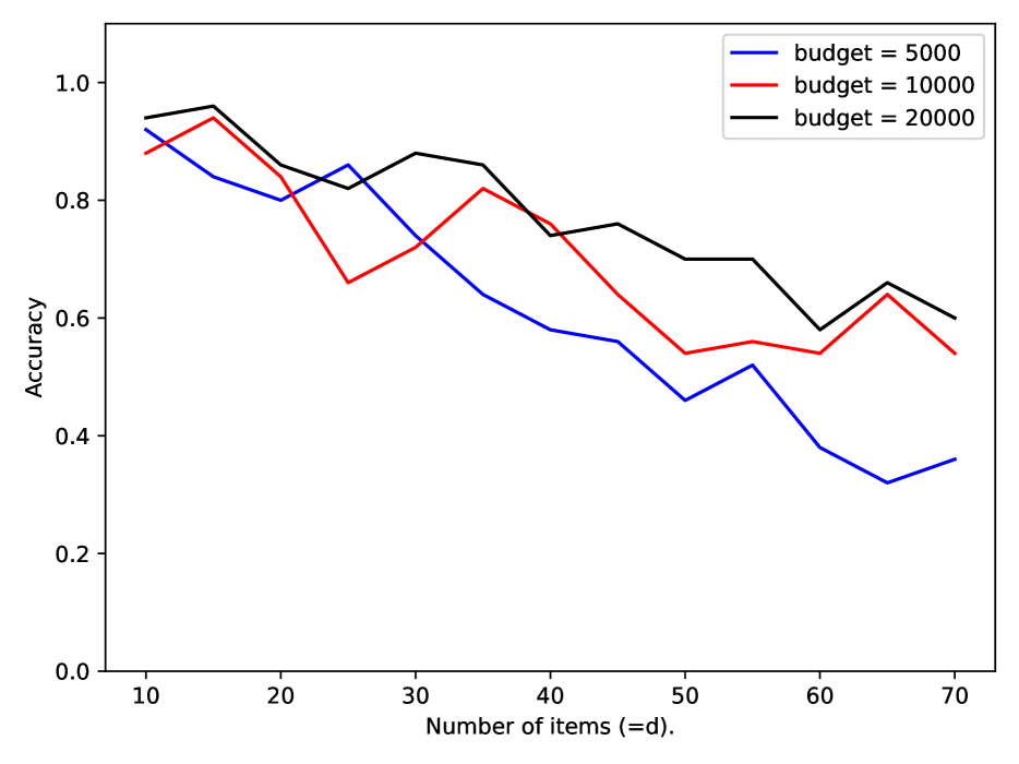
Figure 2: The percentage of the best actions correctly identified by the CSA algorithm in the knapsack problem with different budgets. The horizontal axis represents the number of items $d$. We ran the experiments fifty times for each $d$.

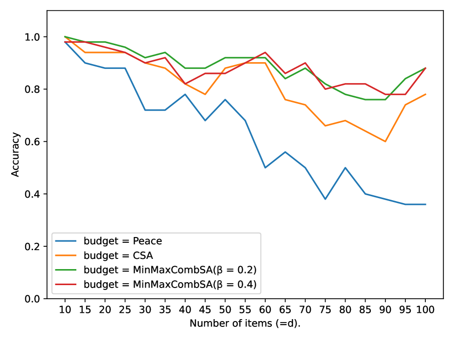
Figure 3: Comparison of the percentage of the best actions correctly identified by the CSA, Minimax-CombSAR, and Peace algorithms. The horizontal axis represents the number of items $d$. We ran the experiments fifty times for each $d$.

Here, we assume $|\mathcal{A}|$ is exponentially large in $d$. Therefore, we can not use the Minimax-CombSAR and the Peace algorithm since they have to enumerate all the possible actions. Here, we see how many times out of 50 experiments the CSA algorithm identified the best action.

For our experiment, we generated the weight of each item $s$, $w_{s}$, uniformly from $\{1,2,\ldots,200\}$. For each item $s$, we generated $v_{s}$ as $v_{s}=w_{s}\times x$, where $x$ is a uniform sample from $[1.0,1.1]$. The capacity of the knapsack was $W=200$. Each time we chose an item $s$, we observed a value $v_{s}+\epsilon$ where $\epsilon$ is a noise from $\mathcal{N}(0,1)$. We set $R=1$. We show the result in Figure 2. The larger the dimension $d$ is, and the smaller the budget $T$ is, the fewer times the optimal actions are correctly identified, which is consistent with the theoretical result of Theorem 2.

6.2 When $|\mathcal{A}|$ is Polynomial in $d$.

Here, we assume that we have prior knowledge of the rewards of arms, i.e., knowledge of the values of the items. We assumed that we know each $v_{s}$ is in $[w_{s},1.1\times w_{s}]$, and used this prior knowledge to generate the action class $\mathcal{A}$ in the following procedure. We first generated a vector $\boldsymbol{v}^{\prime}$ whose $s$-th element $v^{\prime}_{s}$ was uniformly sampled from $[w_{s},1.1\times w_{s}]$, and then solved the knapsack problem with $v^{\prime}_{s}$ and added the obtained solution $\boldsymbol{\pi}$ to $\mathcal{A}$. We repeated this 2000 times; therefore $|\mathcal{A}|\leq 2000$. In this experiment, the budget was $T=50000$. For the Minimax-CombSAR algorithm, we set $\beta=0.2,0.4$. We ran forty experiments for each $d\in\{10,15,\ldots,100\}$. We showed the result in Figure 3. We can see that the Minimax-CombSAR algorithm outperforms the other two algorithms for almost every $d$. Also, the CSA algorithm outperforms the Peace algorithm for almost every $d$.

7 Conclusion

In this paper, we studied the fixed-budget R-CPE-MAB. We first introduced the CSA algorithm, which is the first algorithm that can identify the best action even when the size of the action class is exponentially large with respect to the number of arms. However, it still has an extra logarithmic term in the exponent. Then, we proposed an optimal algorithm named the Minimax-CombSAR algorithm, which, although it is applicable only when the action class is polynomial, matches a lower bound. We showed that both of the algorithms outperform the existing methods.

Checklist

The checklist follows the references. For each question, choose your answer from the three possible options: Yes, No, Not Applicable. You are encouraged to include a justification to your answer, either by referencing the appropriate section of your paper or providing a brief inline description (1-2 sentences). Please do not modify the questions. Note that the Checklist section does not count towards the page limit. Not including the checklist in the first submission won’t result in desk rejection, although in such case we will ask you to upload it during the author response period and include it in camera ready (if accepted).

In your paper, please delete this instructions block and only keep the Checklist section heading above along with the questions/answers below.

1. For all models and algorithms presented, check if you include:

   1. A clear description of the mathematical setting, assumptions, algorithm, and/or model. [Yes]

   2. An analysis of the properties and complexity (time, space, sample size) of any algorithm. [Yes]

   3. (Optional) Anonymized source code, with specification of all dependencies, including external libraries. [Yes]

2. For any theoretical claim, check if you include:

   1. Statements of the full set of assumptions of all theoretical results. [Yes]

   2. Complete proofs of all theoretical results. [Yes]

   3. Clear explanations of any assumptions. [Yes]

3. For all figures and tables that present empirical results, check if you include:

   1. The code, data, and instructions needed to reproduce the main experimental results (either in the supplemental material or as a URL). [Yes]

   2. All the training details (e.g., data splits, hyperparameters, how they were chosen). [Yes]

   3. A clear definition of the specific measure or statistics and error bars (e.g., with respect to the random seed after running experiments multiple times). [Yes]

   4. A description of the computing infrastructure used. (e.g., type of GPUs, internal cluster, or cloud provider). [Yes]

4. If you are using existing assets (e.g., code, data, models) or curating/releasing new assets, check if you include:

   1. Citations of the creator If your work uses existing assets. [Yes]

   2. The license information of the assets, if applicable. [Not Applicable]

   3. New assets either in the supplemental material or as a URL, if applicable. [Yes]

   4. Information about consent from data providers/curators. [Yes]

   5. Discussion of sensible content if applicable, e.g., personally identifiable information or offensive content. [Not Applicable]

5. If you used crowdsourcing or conducted research with human subjects, check if you include:

   1. The full text of instructions given to participants and screenshots. [Not Applicable]

   2. Descriptions of potential participant risks, with links to Institutional Review Board (IRB) approvals if applicable. [Not Applicable]

   3. The estimated hourly wage paid to participants and the total amount spent on participant compensation. [Not Applicable]

Appendix A Proof of Theorem 1

Here, we prove Theorem 1. For the reader’s convenience, we restate the Theorem. See 1 We follow a similar discussion to Carpentier and Locatelli, (2016). This is a lower bound that will hold in the much easier problem where the learner knows that the bandit setting she is facing is one of only $d$ given bandit settings. This lower bound ensures that even in this much simpler case, the learner will make a mistake.

Let $\mathcal{N}(\mu,1)$ denote the Gaussian distribution of mean $\mu$ and unit variance. For any $k\in[d]$, we write $\nu_{k}:=\mathcal{N}\left(\mu_{k},1\right)$. Also, for any $k\in[d]$, we define $\nu^{\prime}_{k}$ as follows:

$$\nu^{\prime}_{k}:=\left\{\begin{array}[]{lll}\mathcal{N}(\mu_{k}+2\Delta_{k},1)&(\mathrm{if}\ \pi^{*}_{k}<\pi_{k}^{(k)})\\ \mathcal{N}(\mu_{k}-2\Delta_{k},1)&(\mathrm{if}\ \pi^{*}_{k}>\pi_{k}^{(k)})\end{array}.\right.$$

Recall that $\Delta_{k}=\frac{\boldsymbol{\mu}^{\top}\left(\boldsymbol{\pi}^{*}-\boldsymbol{\pi}^{(k)}\right)}{\left|\pi_{k}^{*}-\pi^{(k)}_{k}\right|}$ and $\boldsymbol{\pi}^{(k)}=\mathop{\rm arg~{}min}\limits_{\boldsymbol{\pi}\neq\boldsymbol{\pi}^{*}}\frac{\boldsymbol{\mu}^{\top}\left(\boldsymbol{\pi}^{*}-\boldsymbol{\pi}\right)}{\left|\pi^{*}_{k}-\pi_{k}\right|}$.

For any $s\in[d]$, we define the product distributions $\mathcal{G}^{s}$ as $\nu_{1}^{s}\otimes\cdots\otimes\nu_{d}^{s}$, where for $1\leq k\leq d$,

$$\nu^{s}_{k}:=\nu_{k}\mathbf{1}\left[k\neq s\right]+\nu^{\prime}_{k}\mathbf{1}\left[k=s\right].$$ (18)

The bandit problem associated with distribution $\mathcal{G}^{s}$, and that we call “the bandit problem $s$” is such that, for any $1\leq k\leq d$, arm $k$ has distribution $\nu^{s}_{k}$, i.e., all arms have distribution $\nu_{k}$ except for arm $s$ that has distribution $\nu^{\prime}_{k}$. We denote by $\boldsymbol{\mu}^{(s)}$ the vector of expected rewards of bandit problem $s$, i.e., $\mu^{(s)}_{k}=\mu_{k}$ for $k\neq s$, $\mu^{(s)}_{k}=\mu_{k}+2\Delta_{k}$ for $k=s$ and $\pi^{*}_{k}<\pi_{k}^{(k)}$, $\mu^{(s)}_{k}=\mu_{k}-2\Delta_{k}$ for $k=s$ and $\pi^{*}_{k}>\pi_{k}^{(k)}$. For any $1\leq s\leq d$, $\mathbb{P}_{s}:=\mathbb{P}_{\left(\mathcal{G}^{s}\right)^{\otimes T}}$ for the probability distribution of the bandit problem $s$ according to all the samples that a strategy could possibly collect up to horizon $T$, i.e., according to the samples $(X_{k,u})_{1\leq k\leq d,1\leq u\leq T}\sim\left(\mathcal{G}^{s}\right)^{\otimes T}$. Also, we define $\mathbb{P}_{0}:=\mathbb{P}_{\left(\mathcal{G}^{0}\right)^{\otimes T}}$, where $\mathcal{G}^{0}:=\nu_{1}\otimes\cdots\otimes\nu_{d}$.

In the bandit problem $s$, $\boldsymbol{\pi}^{*}$ is no longer the best action since the difference of the expected reward between $\boldsymbol{\pi}^{*}$ and $\boldsymbol{\pi}^{(s)}$ is

$$\sum_{e\in[d]\setminus s}\mu_{e}(\pi^{*}_{e}-\pi_{e}^{(s)})-2\Delta_{s}\times\left|\pi^{*}_{s}-\pi_{s}^{(s)}\right|$$ (19)

$$\leq -\boldsymbol{\mu}^{\top}\left(\boldsymbol{\pi}^{*}-\boldsymbol{\pi}^{(s)}\right)<0.$$

We denote by $\boldsymbol{\pi}^{*,(s)}$ the best action in the bandit problem $s$.

Now, we prove Theorem LABEL:LowerBoundTheorem.

Step 1: Definition of KL-divergence

For two distributions $\nu$ and $\nu^{\prime}$ defined on $\mathbb{R}$, and that are such that $\nu$ is absolutely continuous with respect to $\nu^{\prime}$, we write

$$\mathrm{KL}(\nu,\nu^{\prime})=\int_{\mathbb{R}}\log\left(\frac{d\nu(x)}{d\nu^{\prime}(x)}\right)d\nu(x),$$ (20)

for the Kullback Leibler divergence between distribution $\nu$ and $\nu^{\prime}$. For any $k\in[d]$, let us write

$$\mathrm{KL}_{k}\triangleq\mathrm{KL}(\nu_{k},\nu^{\prime}_{k})=\frac{1}{2}\left(\mu_{a}-\mu_{b}\right)^{2}.$$ (21)

for the Kullback-Leibler divergence between two Gaussian distributions $\mathcal{N}(\mu_{a},1)$ and $\mathcal{N}(\mu_{b},1)$.

Let $1\leq t\leq T$. Also, let us fix $e\in[d]$, and think of bandit instance $e$. We define the quantity:

$$\widehat{\mathrm{KL}}_{s,t} = \frac{1}{t}\sum_{u=1}^{t}\log\left(\frac{d\nu_{s}}{d\nu^{\prime}_{s}}\left(X_{s,u}\right)\right)$$ (22)

$$= \begin{cases}\frac{1}{t}\sum_{u=1}^{t}-\Delta_{s}\left(X_{s,u}-\mu_{s}-2\Delta_{s}\right)&\text{if$\pi^{*}_{s}>\pi^{(s)}_{s}$ and $e\neq s$,}\\ \frac{1}{t}\sum_{u=1}^{t}\Delta_{s}\left(X_{s,u}-\mu_{s}+2\Delta_{s}\right)&\text{if $\pi^{*}_{s}<\pi^{(s)}_{s}$and $e\neq s$,}\\ 0&\text{if $e=s$}\end{cases}$$

where $X_{s,u}\sim_{\mathrm{i.i.d}}\nu_{s}^{e}$ for any $u\leq t$.

Next, let us define the following event:

$$\xi=\left\{\forall 1\leq s\leq d,\forall 1\leq t\leq T,\left|\widehat{\mathrm{KL}}_{s,t}\right|-\mathrm{KL}_{s}\leq\sqrt{2\Delta_{s}^{2}\frac{\log(12Td)}{t}}\right\}.$$ (23)

The following lemma shows a concentration bound for $\left|\widehat{\mathrm{KL}}_{s,t}\right|$.

Lemma 1.

It holds that

$${\Pr}_{e}\left[\xi\right]\geq\frac{5}{6}$$ (24)

Proof.

When $e=s$, $\left|\widehat{\mathrm{KL}}_{s,t}\right|-\mathrm{KL}_{s}\leq\sqrt{2\Delta_{s}^{2}\frac{\log(12Td)}{t}}$ holds for any $t$. Therefore, we think of $e\neq s$. Since $X_{s,t}$ is a $1$-sub-Gaussian random variable, we can see that $\widehat{\mathrm{KL}}_{s,t}$ is a $\frac{{\Delta_{s}}^{2}}{t}$-sub-Gaussian random variable from (22). We can apply the Hoeffding’s inequality to this quantity, and we have that with probability larger than $1-\frac{1}{6dT}$,

$$\left|\widehat{\mathrm{KL}}_{s,t}\right|-\mathrm{KL}_{s}\leq\sqrt{\frac{2\Delta_{s}^{2}\log(12Td)}{t}}$$ (25)

∎

Step2: A change of measure

Let $\mathcal{ALG}$ denote the active strategy of the learner, that returns some action $\boldsymbol{\pi}_{\mathrm{out}}$ after pulling arms $T$ times in total. Let $(T_{s})_{1\leq s\leq T}$ denote the number of samples collected by $\mathcal{ALG}$ on each arm. These quantities are stochastic but it holds that $\sum_{s=1}^{d}T_{s}=T$. For any $1\leq s\leq d$, let us write

$$t_{s}=\mathbb{E}_{0}[T_{s}].$$ (26)

It holds also that $\sum_{s=1}^{d}t_{s}=T$.

We recall the change of measure identity (Audibert et al.,, 2010), which states that for any measurable event $\mathcal{E}$ and for any $1\leq s\leq d$,

$${\Pr}_{s}\left[\mathcal{E}\right]=\mathbb{E}_{0}\left[\mathbbm{1}\left[\mathcal{E}\right]\exp\left(-T_{s}\widehat{\mathrm{KL}}_{s,T_{s}}\right)\right],$$ (27)

where $\mathbbm{1}$ denotes the indicator function.

Then, we consider the following event:

$$\mathcal{E}_{s}=\left\{\boldsymbol{\pi}_{\mathrm{out}}=\boldsymbol{\pi}^{*}\right\}\cap\left\{\xi\right\}\cap\left\{T_{s}\leq 6t_{s}\right\},$$ (28)

i.e., the event where the algorithm outputs action $\boldsymbol{\pi}^{*}$ at the end, where $\xi$ holds, and where the number of times arm $s$ is pulled is smaller than $6t_{s}$. From (28), we have

$${\Pr}_{s}[\mathcal{E}_{s}] = \mathbb{E}_{0}\left[\mathbbm{1}\left[\mathcal{E}_{s}\right]\exp\left(-T_{s}\widehat{\mathrm{KL}}_{s,T_{s}}\right)\right]$$ (29)

$$\geq \mathbb{E}_{0}\left[\mathbbm{1}\left[\mathcal{E}_{s}\right]\exp\left(-T_{s}\mathrm{KL}_{s}-\sqrt{2T_{s}\Delta_{s}^{2}\log(12Td)}\right)\right]$$ (30)

$$\geq \mathbb{E}_{0}\left[\mathbbm{1}\left[\mathcal{E}_{s}\right]\exp\left(-6t_{s}\mathrm{KL}_{s}-\sqrt{2T\Delta_{s}^{2}\log(12Td)}\right)\right]$$ (31)

$$\geq \exp\left(-6t_{s}\mathrm{KL}_{s}-\sqrt{2T\Delta_{s}^{2}\log(12Td)}\right){\Pr}_{0}\left[\mathcal{E}_{s}\right],$$ (32)

since on $\mathcal{E}_{s}$, we have that $\xi$ holds and that $T_{s}\leq 6t_{s}$, and $\mathbb{E}_{0}\left[\widehat{\mathrm{KL}}_{s,t}\right]=\mathrm{KL}_{s}$ for any $t\leq T$.

Step 3: Lower bound on $\Pr_{0}\left[\mathcal{E}_{1}\right]$ for any reasonable algorithm
Assume that the algorithm $\mathcal{ALG}$ is a $\delta$-correct algorithm. Then, we have ${\Pr}_{0}\left[\boldsymbol{\pi}_{\mathrm{out}}\neq\boldsymbol{\pi}^{*}\right]\leq\delta$. From the Markov’s inequality, we have

$${\Pr}_{0}[T_{s}\geq 6t_{s}]\leq\frac{\mathbb{E}_{0}T_{s}}{6t_{s}}=\frac{1}{6},$$ (33)

since $\mathbb{E}_{0}\left[T_{s}\right]=t_{s}$ for algorithm $\mathcal{ALG}$.

Combining Lemma 1, (33), and the fact that $\mathcal{ALG}$ is a $\delta$-correct algorithm, by the union bound, we have

$${\Pr}_{0}\left[\mathcal{E}_{s}\right]\geq 1-\left(1/6+\delta+1/6\right)=\frac{2}{3}-\delta.$$ (34)

This fact combined with (32), (21), and the fact that ${\Pr}_{s}\left[\boldsymbol{\pi}_{\mathrm{out}}\neq\boldsymbol{\pi}^{*,(s)}\right]\geq\Pr_{s}\left[\mathcal{E}_{s}\right]$, we have

$${\Pr}_{s}\left[\boldsymbol{\pi}_{\mathrm{out}}\neq\boldsymbol{\pi}^{*,(s)}\right] \geq \left(\frac{2}{3}-\delta\right)\exp\left(-6t_{s}\mathrm{KL}_{s}-\sqrt{2T\Delta_{s}^{2}\log(12Td)}\right)$$

$$= \left(\frac{2}{3}-\delta\right)\exp\left(-12t_{s}\left(\Delta_{s}\right)^{2}-\sqrt{2T\Delta_{s}^{2}\log(12Td)}\right)$$

since $\mathrm{KL}_{s}=2\Delta_{s}^{2}$.

Step 4: Conclusion. Since $\mathbf{H}=\sum\limits_{s=1}^{d}\left(\frac{1}{\Delta_{s}}\right)^{2}$ and $\sum\limits_{s=1}^{d}t_{s}=T$, there exists $e\in[d]$ such that

$$t_{e}\leq\frac{T}{\mathbf{H}\Delta_{e}^{2}},$$ (35)

as the contradiction yields an immediate contradiction. For this $e$, it holds by (A) that

$${\Pr}_{e}\left[\boldsymbol{\pi}_{\mathrm{out}}\neq\boldsymbol{\pi}^{*,(e)}\right]\geq\left(\frac{2}{3}-\delta\right)\exp\left(-12\frac{T}{\mathbf{H}}-2\sqrt{T\Delta_{e}^{2}\log(6Td)}\right).$$ (36)

This concludes the proof.

Appendix B How to construct COracles

Here, we show how to construct COracles once $\boldsymbol{\mu}$ and $\boldsymbol{S}(t)$ are given for some specific combinatorial problems.

B.1 COracle for the Knapsack Problem

Here, we show that we can construct the COracle for the knapsack problem by calling the offline oracle once. Let $\boldsymbol{S}^{1}(t)$ be the set that collects only the first component of each of all elements in $\boldsymbol{S}(t)$. Also, let $W_{\mathrm{done}}=\sum\limits_{(e,x)\in\boldsymbol{S}(t)}xw_{e}$. If $W-W_{\mathrm{done}}<0$, the COracle outputs $\perp$. Otherwise, we call the offline oracle and solve the following optimization problem:

$$\begin{array}[]{ll@{}ll}\text{maximize}_{\boldsymbol{\xi}}&\sum\limits_{s\in[d]\setminus\boldsymbol{S}^{1}(t)}\mu_{s}\xi_{s}&\\ \\ \text{subject to}&\sum\limits_{s\in\boldsymbol{S}^{1}(t)}\xi_{s}w_{s}\leq W-W_{\mathrm{done}}.&\end{array}$$

Then, we return $\mathrm{COracle}(\boldsymbol{\mu},\boldsymbol{S}(t))=\boldsymbol{S}(t)\cup\boldsymbol{\xi}$.

B.2 COracle for the Optimal Transport Problem

Here, in Algorithm 3, we show the COracle for the optimal transport problem, which calls the offline oracle once. First, let us define $\boldsymbol{S}^{1}(t)$ as the set that collects only the first element of each of all elements in $\boldsymbol{S}(t)$. Then, let us define $\boldsymbol{\pi}^{\mathrm{CO}}$ as the final output of the COracle. Also, let us define $\boldsymbol{s}^{\prime}$ and $\boldsymbol{d}^{\prime}$ as follows:

$$\forall i\in[m],j\in[n],x\in\texttt{POSSIBLE-PI}((i,j)),\ {s}^{\prime}_{i}=\left\{\begin{array}[]{ll}x&(\mathrm{if}\ ((i,j),x)\in\boldsymbol{S}(t),\\ 0&(\mathrm{otherwise}),\\ \end{array}\right.$$ (39)

and

$$\forall i\in[m],j\in[n],x\in\texttt{POSSIBLE-PI}((i,j)),\ {d}^{\prime}_{j}=\left\{\begin{array}[]{ll}x&(\mathrm{if}\ ((i,j),x)\in\boldsymbol{S}(t),\\ 0&(\mathrm{otherwise}).\\ \end{array}\right.$$ (42)

Also, let us define $\boldsymbol{\pi}^{\prime}\in\mathbb{R}^{m\times n}$ whose $(i,j)$-th element is defined as follows:

$$\forall i\in[m],j\in[n],x\in\texttt{POSSIBLE-PI}((i,j)),\ \boldsymbol{\pi}^{\prime}_{ij}=\left\{\begin{array}[]{ll}x&(\mathrm{if}\ ((i,j),x)\in\boldsymbol{S}(t),\\ 0&(\mathrm{otherwise}).\\ \end{array}\right.$$ (45)

Intuitively, for any $((i,j),x)\in\boldsymbol{S}(t)$, we have to send resources from supplier $i$ to demander $j$ for a value of $s^{\prime}_{i}(=d^{\prime}_{j})$. This means that we have resources of $s_{i}-s^{\prime}_{i}$ left to send from supplier $i$, and $d_{j}-d^{\prime}_{j}$ left to send to demander $j$. Since we can not send a negative value of resources, $s_{i}-s^{\prime}_{i}\geq 0$ and $d_{j}-d^{\prime}_{j}\geq 0$ have to be satisfied.

From the above discussion, we can formally write $\boldsymbol{\pi}^{\mathrm{CO}}$ as follows:

$$\boldsymbol{\pi}^{\mathrm{CO}}=\left\{\begin{array}[]{ll}\sum_{i,j}\pi^{\prime}_{ij}\gamma_{ij}+\mathop{\rm arg~{}min}\limits_{\boldsymbol{\pi}^{\prime\prime}\in\mathcal{G}\left(\boldsymbol{s}-\boldsymbol{s}^{\prime},\boldsymbol{d}-\boldsymbol{d}^{\prime}\right)}\sum_{i,j}\pi^{\prime\prime}_{ij}\gamma^{\prime}_{ij}&(\text{ if there is no negative value in neither $\boldsymbol{s}-\boldsymbol{s}^{\prime}$ nor $\boldsymbol{d}-\boldsymbol{d}^{\prime}$}),\\ \perp&(\mathrm{otherwise}).\\ \end{array}\right.$$ (48)

Here, $\boldsymbol{\gamma}^{\prime}$ is defined as

$$\forall i\in[m],j\in[n],x\in\texttt{POSSIBLE-PI}((i,j)),\ {\gamma}^{\prime}_{ij}=\left\{\begin{array}[]{ll}-\infty&(\mathrm{if}\ ((i,j),x)\in\boldsymbol{S}(t),\\ \gamma_{ij}&(\mathrm{otherwise}),\\ \end{array}\right.$$ (51)

to not let $\boldsymbol{\pi}^{\mathrm{CO}}$ send materials more than the amount determined by $\boldsymbol{S}(t)$.

Algorithm 3 COracle for the Optimal Transport Problem

0:  Cost matrix: $\boldsymbol{\gamma}$, supply vector $\boldsymbol{s}\in\mathbb{R}^{m}$, demand vector $\boldsymbol{d}\in\mathbb{R}^{n}$, $\boldsymbol{S}(t)$

1:  $\boldsymbol{\pi}^{\prime}\leftarrow\boldsymbol{0}^{m\times n}$

2:  for $((i,j),x)$ in $\boldsymbol{S}(t)$ do

3:     $\pi^{\prime}_{ij}\leftarrow x$

4:     $s_{i}\leftarrow s_{i}-x$

5:     $d_{j}\leftarrow d_{j}-x$

6:     $\gamma_{ij}\leftarrow-\infty$

7:     if $s_{i}<0$ or $d_{j}<0$ then

8:        Return $\perp$

9:     end if

10:  end for

11:  Compute $\boldsymbol{\pi}^{\prime\prime}=\mathop{\rm arg~{}min}\limits_{\boldsymbol{\pi}\in\mathcal{G}(\boldsymbol{s},\boldsymbol{d})}\sum_{i,j}\pi_{ij}\gamma_{ij}$ using the offline oracle

12:  Return $\boldsymbol{\pi}^{\mathrm{CO}}=\boldsymbol{\pi}^{\prime}+\boldsymbol{\pi}^{\prime\prime}$

B.3 COracle for a General Case When $K(=|\mathcal{A}|)=\mathrm{poly}(d)$

Here, we show the time complexity of the COracle when the size of the action class is polynomial in $d$. If $\mathcal{A}_{S}$ is an empty set, the COracle returns $\perp$. Otherwise, we return $\boldsymbol{\pi}^{\mathrm{return}}=\mathop{\rm arg~{}max}\limits_{\boldsymbol{\pi}\in\mathcal{A}_{S}}\boldsymbol{\mu}^{\top}\boldsymbol{\pi}$. The time complexity to construct $\mathcal{A}_{S}$ is $\mathcal{O}(dK)$. This is because, for each action $\boldsymbol{\pi}\in\mathcal{A}$, we check every dimension to see if $\boldsymbol{\pi}\in\mathcal{A}_{S}$. Then, the time complexity of finding $\boldsymbol{\pi}^{\mathrm{return}}$ from $\mathcal{A}_{S}$ is $\mathcal{O}(K\log K)$. Therefore the time complexity of the COracle is $\mathcal{O}\left(dK+K\log K\right)$.

Appendix C Proof of Theorem 2

Here, we prove Theorem 2. We first introduce some notions that are useful to prove it. Then, we show some preparatory lemmas that are needed to prove Theorem 2.

C.1 Preparatories

Let us introduce some notions that are useful to prove the theorem.

C.1.1 Arm-Value Pair

We define an arm-value pair set $\boldsymbol{M}(\boldsymbol{\pi})\subset[d]\times\mathbb{R}$ of $\boldsymbol{\pi}$ as follows:

$$\boldsymbol{M}(\boldsymbol{\pi})=\{(e,\pi_{e})\ |\ \forall e\in[d]\}.$$

Also, we define the arm-value pair family $\mathcal{M}$ as follows:

$$\mathcal{M}=\{\boldsymbol{M}(\boldsymbol{\pi})\ |\ \forall\boldsymbol{\pi}\in\mathcal{A}\}.$$

For any arm-value pair set $\boldsymbol{M}\in\mathcal{M}$, we denote by $M_{e}$ the second component of the ordered pair whose first component is $e$, i.e., $M_{e}=x$ for any $(e,x)\in\boldsymbol{M}$. Also, we call $M_{e}$ the $e$-th element of $\boldsymbol{M}$.

For any two different arm-value pair set $\boldsymbol{M},\boldsymbol{M}^{\prime}\in\mathcal{M}$, we define an operator $\boxminus$ such that the $e$-th element of $\boldsymbol{M}^{\prime}\boxminus\boldsymbol{M}\subset[d]\times\mathbb{R}$, $(\boldsymbol{M}^{\prime}\boxminus\boldsymbol{M})_{e}$, is defined as follows:

$$(\boldsymbol{M}^{\prime}\boxminus\boldsymbol{M})_{e}=\left\{\begin{array}[]{lll}M^{\prime}_{e}-M_{e}&(\mathrm{if}\ M^{\prime}_{e}>M_{e})\\ 0&(\mathrm{if}\ M^{\prime}_{e}\leq M_{e})\end{array}.\right.$$ (54)

C.1.2 Exchange Class

We define an exchange set $b$ as an ordered pair of sets $b=(\boldsymbol{b}^{+},\boldsymbol{b}^{-})$, where $\boldsymbol{b}^{+},\boldsymbol{b}^{-}\subset[d]\times\mathbb{R}\setminus\{0\}$. We say $\boldsymbol{b}^{+}$ (or $\boldsymbol{b}^{-}$) has as $e$-changer if it has an element whose first component is $e$. For any $\boldsymbol{b}^{+}$ (or $\boldsymbol{b}^{-}$), we denote by $b^{+}_{e}$ the second component of the ordered pair whose first component is $e$, i.e., $b^{+}_{e}=x$ for any $(e,x)\in\boldsymbol{b}^{+}$. Also, for any $b=(\boldsymbol{b}^{+},\boldsymbol{b}^{-})$, we do not let both $\boldsymbol{b}^{+}$ and $\boldsymbol{b}^{-}$ have $e$-changers.

Next, for any arm-value pair set $\boldsymbol{M}\in\mathcal{M}$, exchange set $b=(\boldsymbol{b}^{+},\boldsymbol{b}^{-})$, and $e\in[d]$, we define operator $\oplus$ such that the $e$-the element of $\boldsymbol{M}\oplus b\subset[d]\times\mathbb{R}$, $(\boldsymbol{M}\oplus b)_{e}$, is defined as follows:

$$(\boldsymbol{M}\oplus b)_{e}=\left\{\begin{array}[]{lll}M_{e}+b^{+}_{e}&(\mathrm{if}\ \boldsymbol{b}^{+}\ \mathrm{has\ an\ \mathit{e-}changer})\\ M_{e}-b^{-}_{e}&(\mathrm{if}\ \boldsymbol{b}^{-}\ \mathrm{has\ an\ \mathit{e-}changer})\\ M_{e}&(\mathrm{if\ neither}\ \boldsymbol{b}_{+}\ \mathrm{nor}\ \boldsymbol{b}^{-}\ \mathrm{has\ an\ \mathit{e-}changer})\\ \end{array}.\right.$$ (55)

Similarly, for any arm-value pair set $\boldsymbol{M}\in\mathcal{M}$, exchange set $b=(\boldsymbol{b}^{+},\boldsymbol{b}^{-})$, and $e\in[d]$, we define operator $\ominus$ such that the $e$-the element of $\boldsymbol{M}\ominus b\subset[d]\times\mathbb{R}$, $(\boldsymbol{M}\ominus b)_{e}$, is defined as follows:

$$(\boldsymbol{M}\ominus b)_{e}=\left\{\begin{array}[]{lll}M_{e}-b^{+}_{e}&(\mathrm{if}\ \boldsymbol{b}^{+}\ \mathrm{has\ an\ \mathit{e-}changer})\\ M_{e}+b^{-}_{e}&(\mathrm{if}\ \boldsymbol{b}^{-}\ \mathrm{has\ an\ \mathit{e-}changer})\\ M_{e}&(\mathrm{if\ neither}\ \boldsymbol{b}^{+}\ \mathrm{nor}\ \boldsymbol{b}^{-}\ \mathrm{has\ an\ \mathit{e-}changer})\\ \end{array}.\right.$$ (56)

We call a collection of exchange sets $\mathcal{B}$ an exchange class for $\mathcal{M}$ if $\mathcal{B}$ satisfies the following property. For any $\boldsymbol{M},\boldsymbol{M}^{\prime}\in\mathcal{M}$ and $e\in[d]$, where $(\boldsymbol{M}\boxminus\boldsymbol{M}^{\prime})_{e}>0$, there exists an exchange set $b=(\boldsymbol{b}^{+},\boldsymbol{b}^{-})\in\mathcal{B}$ that satisfies the following five constraints: (a) $b^{-}_{e}=(\boldsymbol{M}\boxminus\boldsymbol{M}^{\prime})_{e}$ (b) $\boldsymbol{b}^{+}\subseteq\boldsymbol{M}^{\prime}\boxminus\boldsymbol{M}$, (c) $\boldsymbol{b}^{-}\subseteq\boldsymbol{M}\boxminus\boldsymbol{M}^{\prime}$, (d)$(\boldsymbol{M}\oplus b)\in\mathcal{M}$ and (e) $(\boldsymbol{M}^{\prime}\ominus b)\in\mathcal{M}$.

For any $\boldsymbol{a}\subset[d]\times\mathbb{R}$, let $a_{e}$ denote the second component of the ordered pair whose first component is $e$, i.e., $a_{e}=x$ for any $(e,x)\in\boldsymbol{a}$. Then, let $\boldsymbol{\chi}(\boldsymbol{a})\in\mathbb{R}^{d}$ denote the vector defined as follows:

$$\chi_{e}(\boldsymbol{a})=\left\{\begin{array}[]{lll}a_{e}&(\text{if $\boldsymbol{a}$ has an element whose first component is $e$ })\\ 0&(\text{otherwise})\end{array}.\right.$$ (59)

Also, for any exchange set $b$, we define $\boldsymbol{\chi}(b)=\boldsymbol{\chi}(\boldsymbol{b}^{+})-\boldsymbol{\chi}(\boldsymbol{b}^{-})$.

C.2 Preparatory Lemmas

Here, let us introduce some lemmas that are useful to prove the theorem. Below, we define $\boldsymbol{M}^{*}=\boldsymbol{M}(\boldsymbol{\pi}^{*})$.

Lemma 2 (Interpolation Lemma).

Let $\mathcal{B}$ be an exchange class of $\mathcal{M}$, and $\boldsymbol{M},\boldsymbol{M}^{\prime}$ be two different members of $\mathcal{M}$. Then, for any $e\in\{s\in[d]\ |\ M_{s}\neq M^{\prime}_{s}\}$, there exists an exchange set $b=(\boldsymbol{b}^{+},\boldsymbol{b}^{-})\in\mathcal{B}$, which satisfies the following five constraints: (a) $b^{-}_{e}=(\boldsymbol{M}\boxminus\boldsymbol{M}^{\prime})_{e}$ or $b^{+}_{e}=(\boldsymbol{M}^{\prime}\boxminus\boldsymbol{M})_{e}$, (b) $\boldsymbol{b}^{-}\subseteq(\boldsymbol{M}\boxminus\boldsymbol{M}^{\prime})$, (c) $\boldsymbol{b}^{+}\subseteq\boldsymbol{M}^{\prime}\boxminus\boldsymbol{M}$, (d) $(\boldsymbol{M}\oplus b)\in\mathcal{M}$ and (e)$(\boldsymbol{M}^{\prime}\ominus b)\in\mathcal{M}$. Moreover, if $\boldsymbol{M}^{\prime}=\boldsymbol{M}^{*}$, then we have

$$\frac{\langle\boldsymbol{\mu},\boldsymbol{\chi}(b)\rangle}{\chi_{e}(b)}\geq\Delta_{e}.$$ (60)

Proof.

We decompose our proof into two cases.

Case (1): $(\boldsymbol{M}\boxminus\boldsymbol{M}^{\prime})_{e}>0$

By the definition of the exchange class, we know that there exists $b=(\boldsymbol{b}^{+},\boldsymbol{b}^{-})\in\mathcal{B}$ which satisfies that there is an $e\in[d]$ where (a) $b^{-}_{e}=(\boldsymbol{M}\boxminus\boldsymbol{M}^{\prime})_{e}$, (b) $\boldsymbol{b}^{-}\subseteq(\boldsymbol{M}\boxminus\boldsymbol{M}^{\prime})$, (c) $\boldsymbol{b}^{+}\subseteq\boldsymbol{M}^{\prime}\boxminus\boldsymbol{M}$, (d) $(\boldsymbol{M}\oplus b)\in\mathcal{M}$ and (e)$(\boldsymbol{M}^{\prime}\ominus b)\in\mathcal{M}$. Therefore the five constraints are satisfied.

Case (2): $(\boldsymbol{M}^{\prime}\boxminus\boldsymbol{M})_{e}>0$

Using the definition of the exchange class, we see that there exists $b=(\boldsymbol{c}^{+},\boldsymbol{c}^{-})\in\mathcal{B}$ such that (a) $c^{-}_{e}=(\boldsymbol{M}^{\prime}\boxminus\boldsymbol{M})_{e}$, (b) $\boldsymbol{c}^{-}\subseteq(\boldsymbol{M}^{\prime}\boxminus\boldsymbol{M})$, (c) $\boldsymbol{c}^{+}\subseteq(\boldsymbol{M}\boxminus\boldsymbol{M}^{\prime})$, (d) $(\boldsymbol{M}\oplus b)\in\mathcal{M}$, and (e) $(\boldsymbol{M}^{\prime}\ominus b)\in\mathcal{M}$. We construct $b=(\boldsymbol{b}^{+},\boldsymbol{b}^{-})$ by setting $\boldsymbol{b}^{+}=\boldsymbol{c}^{-}$ and $\boldsymbol{b}^{-}=\boldsymbol{c}^{+}$. Notice that, by the construction of $b$, we have $\boldsymbol{M}\oplus b=\boldsymbol{M}\ominus c$ and $\boldsymbol{M}^{\prime}\ominus b=\boldsymbol{M}^{\prime}\oplus c$. Therefore, it is clear that $b$ satisfies the five constraints of the lemma.

Next, let us think when $\boldsymbol{M}^{\prime}=\boldsymbol{M}^{*}$ for both cases. Let us consider

$$\boldsymbol{\pi}^{1}=\mathop{\rm arg~{}min}\limits_{\boldsymbol{\pi}\in\mathcal{M}\setminus\boldsymbol{\pi}^{*}}\frac{\langle\boldsymbol{\mu},\boldsymbol{\pi}^{*}-\boldsymbol{\pi}\rangle}{\left|\pi^{*}_{e}-\pi_{e}\right|}.$$ (61)

Note that, by the definition of the G-Gap, we have $\frac{\langle\boldsymbol{\mu},\boldsymbol{\pi}^{*}-\boldsymbol{\pi}^{1}\rangle}{\left|\pi^{*}_{e}-\pi^{1}_{e}\right|}=\Delta_{e}$. We define $\boldsymbol{\pi}^{0}$ such that $\boldsymbol{M}(\boldsymbol{\pi}^{0})=\boldsymbol{M}(\boldsymbol{\pi}^{*})\ominus b$. Note that we already have $\boldsymbol{M}(\boldsymbol{\pi}^{0})\in\mathcal{M}$. We can see that

$$\frac{\langle\boldsymbol{\mu},\boldsymbol{\chi}(b)\rangle}{\left|\chi_{e}(b)\right|}=\frac{\langle\boldsymbol{\mu},\boldsymbol{\pi}^{*}-\boldsymbol{\pi}^{0}\rangle}{\left|\pi^{*}_{e}-\pi^{0}_{e}\right|}\geq\Delta_{e},$$ (62)

where the inequality follows from the definition of G-Gap. ∎

Next, we establish the confidence bounds used for the analysis of the CSA algorithm.

Lemma 3.

Given a phase $t\in[d]$, we define random events $\tau_{t}$ as follows:

$$\tau(t)=\left\{\forall s\in[d]\setminus F(t),|\hat{\mu}_{s}(t)-\mu_{s}|<\frac{\Delta_{(d-t+1)}}{(2+L^{2})U_{\mathcal{A}}}\right\},$$ (63)

where $L=\max_{e\in[d],\boldsymbol{\pi}^{1},\boldsymbol{\pi}^{2},\boldsymbol{\pi}^{3}\in\mathcal{A}}\frac{\left|\pi^{1}_{e}-\pi^{2}_{e}\right|}{\left|\pi^{1}_{e}-\pi^{3}_{e}\right|}$. Then, we have

$$\Pr\left[\bigcap_{t=1}^{d}\tau(t)\right]\geq 1-d^{2}\exp\left(-\frac{T-d}{2\left(2+L^{2}\right)^{2}R^{2}\tilde{\log}(d)U^{2}_{\mathcal{M}}\mathbf{H}_{2}}\right)$$ (64)

Proof.

Fix some $t\in[d]$ and active arm $s\in[d]\setminus F(t)$ of phase $t$. Note that arm $s$ has been pulled for $\tilde{T}(t)$ times during the first $t$ phases. Therefore, by Hoeffding’s inequality, we have

$$\Pr\left[\left|\hat{\mu}_{s}(t)-\mu_{s}\right|\geq\frac{\Delta_{(d-t+1)}}{(2+L^{2})U_{\mathcal{A}}}\right]\leq 2\exp\left(-\frac{\tilde{T}(t)\Delta^{2}_{(d-t+1)}}{2\left(2+L^{2}\right)^{2}R^{2}U^{2}_{\mathcal{A}}}\right).$$ (65)

By plugging the definition of $\tilde{T}(t)$, the quantity $\tilde{T}(t)\Delta^{2}_{(d-t+1)}$ on the right hand side of (65) can be further bounded by

$$\tilde{T}(t)\Delta^{2}_{(d-t+1)} \geq \frac{T-d}{\tilde{\log}(d)(d-t+1)}\Delta^{2}_{(d-t+1)}$$

$$\geq \frac{T-d}{\tilde{\log}(d)\mathbf{H}_{2}},$$

where the last inequality follows from the definition of $\mathbf{H}_{2}=\max_{s\in[d]}\frac{s}{\Delta^{2}_{(s)}}$. By plugging the last equality into (65), we have

$$\Pr\left[\left|\hat{\mu}_{s}(t)-\mu_{s}\right|\geq\frac{\Delta_{(d-t+1)}}{(2+L^{2})U_{\mathcal{A}}}\right]\leq 2\exp\left(-\frac{T-d}{2\left(2+L^{2}\right)^{2}R^{2}\tilde{\log}(d)U^{2}_{\mathcal{A}}\mathbf{H}_{2}}\right).$$ (66)

Using (66) and a union bound for all $t\in[d]$ and all $s\in[d]\setminus F(t)$, we have

$$\Pr\left[\bigcap_{t=1}^{d}\tau(t)\right] \geq 1-2\sum_{t=1}^{d}(d-t+1)\exp\left(-\frac{T-d}{2\left(2+L^{2}\right)^{2}R^{2}\tilde{\log}(d)U^{2}_{\mathcal{A}}\mathbf{H}_{2}}\right)$$

$$\geq 1-d^{2}\exp\left(-\frac{T-d}{2\left(2+L^{2}\right)^{2}R^{2}\tilde{\log}(d)U^{2}_{\mathcal{M}}\mathbf{H}_{2}}\right)$$

∎

The following lemma builds the confidence bound of inner products.

Lemma 4.

Fix a phase $t\in[d]$. Suppose that random event $\tau(t)$ occurs. For any vector $\boldsymbol{a}\in\mathbb{R}^{d}$, we have

$$|\langle\hat{\boldsymbol{\mu}}(t),\boldsymbol{a}\rangle-\langle\boldsymbol{\mu},\boldsymbol{a}\rangle|<\frac{\Delta_{(d-t+1)}}{(2+L^{2})U_{\mathcal{A}}}\|\boldsymbol{a}\|_{1}.$$ (67)

Proof.

Suppose that $\tau_{t}$ occurs. We have

$$|\langle\hat{\boldsymbol{\mu}}(t),\boldsymbol{a}\rangle-\langle\boldsymbol{\mu},\boldsymbol{a}\rangle| = |\langle\hat{\boldsymbol{\mu}}(t)-\boldsymbol{\mu},\boldsymbol{a}\rangle|$$

$$= \left|\sum_{s=1}^{d}(\hat{\mu}_{s}(t)-\mu_{s})a_{s}\right|$$

$$\leq \sum_{s=1}^{d}|\hat{\mu}_{s}(t)-\mu_{s}||a_{s}|$$

$$< \frac{\Delta_{(d-t+1)}}{(2+L^{2})U_{\mathcal{A}}}\sum_{i=1}^{d}|a_{s}|$$

$$= \frac{\Delta_{(d-t+1)}}{(2+L^{2})U_{\mathcal{A}}}\|\boldsymbol{a}\|_{1},$$

where (C.2) follows from the definition of $\tau_{t}$ in (63). ∎

C.3 Main Lemmas

Let $\boldsymbol{R}(t)=\{(e,x)\ |\ \forall e\in[d],\forall x\in\texttt{POSSIBLE-PI(e)},(e,x)\notin\boldsymbol{S}(t)\}$. We begin with a technical lemma that characterizes several useful lemma properties of $\boldsymbol{S}(t)$ and $\boldsymbol{R}(t)$.

Lemma 5.

Fix a phase $t\in[d]$. Suppose that $\boldsymbol{S}(t)\subseteq\boldsymbol{M}^{*}$ and $\boldsymbol{R}(t)\cap\boldsymbol{M}^{*}=\emptyset$. Let $\boldsymbol{M}$ be a set such that $\boldsymbol{S}(t)\subseteq\boldsymbol{M}$ and $\boldsymbol{R}(t)\cap\boldsymbol{M}=\emptyset$. Let $\boldsymbol{a}$ and $\boldsymbol{b}$ be two sets satisfying that $\boldsymbol{a}\subseteq\boldsymbol{M}\setminus\boldsymbol{M}^{*}$, $\boldsymbol{b}\subseteq\boldsymbol{M}^{*}\setminus\boldsymbol{M}$ and $\boldsymbol{a}\cap\boldsymbol{b}=\emptyset$. Then, we have

$\boldsymbol{S}(t)\subseteq\left(\boldsymbol{M}\setminus\boldsymbol{a}\cup\boldsymbol{b}\right)$   and   $\boldsymbol{R}(t)\cap(\boldsymbol{M}\setminus\boldsymbol{a}\cup\boldsymbol{b})=\emptyset$

Proof.

We first prove the first part as follows:

$$\boldsymbol{S}(t)\cap\left(\boldsymbol{M}\setminus\boldsymbol{a}\cup\boldsymbol{b}\right) = \left(\boldsymbol{S}(t)\cap\left(\boldsymbol{M}\setminus\boldsymbol{a}\right)\right)\cup\left(\boldsymbol{S}(t)\cap\boldsymbol{b}\right)$$

$$= \boldsymbol{S}(t)\cap\left(\boldsymbol{M}\setminus\boldsymbol{a}\right)$$

$$= \left(\boldsymbol{S}(t)\cap\boldsymbol{M}\right)\setminus\boldsymbol{a}$$

$$= \boldsymbol{S}(t)\setminus\boldsymbol{a}$$ (70)

$$= \boldsymbol{S}(t),$$ (71)

where (C.3) holds since we have $\boldsymbol{S}(t)\cap\boldsymbol{b}\subseteq\boldsymbol{S}(t)\cap(\boldsymbol{M}^{*}\setminus\boldsymbol{M})\subseteq\boldsymbol{M}\cap(\boldsymbol{M}^{*}\setminus\boldsymbol{M})=\emptyset$; (70) follows from $\boldsymbol{S}(t)\subseteq\boldsymbol{M}$; and (71) follows from $\boldsymbol{a}\subseteq\boldsymbol{M}\setminus\boldsymbol{M}^{*}$ and $\boldsymbol{S}(t)\subseteq\boldsymbol{M}^{*}$ which implies that $\boldsymbol{a}\cap\boldsymbol{S}(t)=\emptyset$. Notice that $\boldsymbol{S}(t)\subseteq(\boldsymbol{M}\setminus\boldsymbol{a}\cup\boldsymbol{b})$.

Then, we proceed to prove the second part in the following

$$\boldsymbol{R}(t)\cap(\boldsymbol{M}\setminus\boldsymbol{a}\cup\boldsymbol{b}) = (\boldsymbol{R}(t)\cap(\boldsymbol{M}\setminus\boldsymbol{a}))\cup(\boldsymbol{R}(t)\cap\boldsymbol{b})$$

$$= \boldsymbol{R}(t)\cap(\boldsymbol{M}\setminus\boldsymbol{a})$$

$$= (\boldsymbol{R}(t)\cap\boldsymbol{M})\setminus\boldsymbol{a}$$

$$= \emptyset\setminus\boldsymbol{a}=\emptyset,$$ (73)

where (C.3) follows from the fact that $\boldsymbol{R}(t)\cap\boldsymbol{b}\subseteq\boldsymbol{R}(t)\cap(\boldsymbol{M}^{*}\setminus M)\subseteq R(t)\cap\boldsymbol{M}^{*}=\emptyset$; and (73) follows from the fact that $\boldsymbol{R}(t)\cap\boldsymbol{M}=\emptyset$.

∎

Let $\hat{\boldsymbol{M}}(t)=\boldsymbol{M}(\hat{\boldsymbol{\pi}}(t))$. The next lemma provides an important insight into the correctness of the CSA algorithm. Informally speaking, suppose that the algorithm does not make an error before phase $t$. Then, we show that, if arm $e$ has a gap $\Delta_{e}$ larger than the “reference gap” $\Delta_{(d-t+1)}$ of phase $t$, then arm $e$ must be correctly clarified by $\hat{\boldsymbol{M}}(t)$, i.e., $M_{e}(t)=M^{*}_{e}$.

Lemma 6.

Fix any phase $t>0$. Suppose that event $\tau_{t}$ occurs. Also, assume that $\boldsymbol{S}(t)\subseteq\boldsymbol{M}^{*}$ and $\boldsymbol{R}(t)\cap\boldsymbol{S}(t)=\emptyset$. Let $e\in[d]\setminus\boldsymbol{F}(t)$ be an active arm. Suppose that $\Delta_{(d-t+1)}\leq\Delta_{e}$. Then, we have $(e,\pi^{*}_{e})\in\boldsymbol{M}^{*}\cap\boldsymbol{S}(t)$.

Proof.

Suppose that $(e,\pi^{*}_{e})\notin(\boldsymbol{M}^{*}\cap\hat{\boldsymbol{M}}(t))$. This is equivalent to the following

$$(e,\pi^{*}_{e})\in(\boldsymbol{M}^{*}\cap\lnot\hat{\boldsymbol{M}}(t))\cup(\lnot\boldsymbol{M}^{*}\cap\hat{\boldsymbol{M}}(t))$$ (74)

(74) can be further rewritten as

$$(e,\pi^{*}_{e})\in(\boldsymbol{M}^{*}\setminus\hat{\boldsymbol{M}}(t))\cup(\hat{\boldsymbol{M}}(t)\setminus\boldsymbol{M}^{*}).$$ (75)

From this assumption, it is easy to see that $\hat{\boldsymbol{M}}(t)\neq\boldsymbol{M}^{*}$. Therefore, we can apply Lemma 2. We know that there exists $b=(\boldsymbol{b}^{+},\boldsymbol{b}^{-})\in\mathcal{B}$ such that (a) ${b}^{-}_{e}=(\hat{\boldsymbol{M}}(t)\boxminus\boldsymbol{M}^{*})_{e}$ or ${b}^{+}_{e}=(\boldsymbol{M}^{*}\boxminus\hat{\boldsymbol{M}}(t))_{e}$, (b) $\boldsymbol{b}^{-}\subseteq(\hat{\boldsymbol{M}}(t)\boxminus\boldsymbol{M}^{*})$, (c) $\boldsymbol{b}^{+}\subseteq\boldsymbol{M}^{*}\boxminus\hat{\boldsymbol{M}}(t)$, (d) $(\hat{\boldsymbol{M}}(t)\oplus b)\in\mathcal{M}$, (e) $(\boldsymbol{M}^{*}\ominus b)\in\mathcal{M}$, and $\frac{\langle\boldsymbol{\mu},\boldsymbol{\chi}(b)\rangle}{\chi_{e}(b)}\geq\Delta_{e}>0$.

Using Lemma 5, we see that $(\hat{\boldsymbol{M}}(t)\oplus b)\cap\boldsymbol{R}(t)=\emptyset$, $\boldsymbol{S}(t)\subseteq(\hat{\boldsymbol{M}}(t)\oplus b)$, and $(\boldsymbol{b}^{+}\cup\boldsymbol{b}^{-})\cap(\boldsymbol{S}(t)\cup\boldsymbol{R}(t))=\emptyset$.

Recall the definition $\hat{\boldsymbol{M}}(t)\in\mathop{\rm arg~{}max}\limits_{\boldsymbol{M}\in\mathcal{M},\boldsymbol{S}(t)\subseteq\boldsymbol{M},\boldsymbol{R}(t)\cap\boldsymbol{M}=\emptyset}\langle\hat{\boldsymbol{\mu}}(t),\boldsymbol{\pi}(\boldsymbol{M})\rangle$ and also recall that $\hat{\boldsymbol{M}}(t)\oplus b\in\mathcal{M}$. Therefore, we obtain that

$$\frac{\langle\hat{\boldsymbol{\mu}}(t),\boldsymbol{\pi}(\hat{\boldsymbol{M}}(t))\rangle}{\chi_{e}(b)}\geq\frac{\langle\hat{\boldsymbol{\mu}},\boldsymbol{\pi}(\hat{\boldsymbol{M}}(t)\oplus b)\rangle}{\chi_{e}(b)}.$$ (76)

On the other hand, we have

$$\frac{\langle\hat{\boldsymbol{\mu}}(t),\boldsymbol{\pi}(\hat{\boldsymbol{M}}(t)\oplus b)\rangle}{\chi_{e}(b)} = \frac{\langle\hat{\boldsymbol{\mu}}(t),\boldsymbol{\pi}(\hat{\boldsymbol{M}}(t))+\boldsymbol{\chi}(b)\rangle}{\chi_{e}(b)}$$

$$= \frac{\langle\hat{\boldsymbol{\mu}}(t),\boldsymbol{\pi}(\hat{\boldsymbol{M}}(t))\rangle}{{\chi_{e}(b)}}+\frac{\langle\hat{\boldsymbol{\mu}}(t),\boldsymbol{\chi}(b)\rangle}{{\chi_{e}(b)}}$$

$$> \frac{\langle\hat{\boldsymbol{\mu}}(t),\boldsymbol{\pi}(\hat{\boldsymbol{M}}(t))\rangle}{{\chi_{e}(b)}}+\frac{\langle\boldsymbol{\mu},\boldsymbol{\chi}(b)\rangle}{{\chi_{e}(b)}}-\frac{\Delta_{(d-t+1)}}{(2+L^{2})U_{\mathcal{A}}}\frac{\|\boldsymbol{\chi}(b)\|}{{\chi_{e}(b)}}$$

$$\geq \frac{\langle\hat{\boldsymbol{\mu}}(t),\boldsymbol{\pi}(\hat{\boldsymbol{M}}(t))\rangle}{{\chi_{e}(b)}}+\frac{\langle\boldsymbol{\mu},\boldsymbol{\chi}(b)\rangle}{{\chi_{e}(b)}}-\frac{\Delta_{e}}{(2+L^{2})U_{\mathcal{A}}}\frac{\|\boldsymbol{\chi}(b)\|}{{\chi_{e}(b)}}$$

$$\geq \frac{\langle\hat{\boldsymbol{\mu}}(t),\boldsymbol{\pi}(\hat{\boldsymbol{M}}(t))\rangle}{{\chi_{e}(b)}}+\frac{\langle\boldsymbol{\mu},\boldsymbol{\chi}(b)\rangle}{{\chi_{e}(b)}}-\frac{\Delta_{e}}{(2+L^{2})}$$ (79)

$$\geq \frac{\langle\hat{\boldsymbol{\mu}}(t),\boldsymbol{\pi}(\hat{\boldsymbol{M}}(t))\rangle}{{\chi_{e}(b)}}+\frac{1+L^{2}}{2+L^{2}}\Delta_{e}$$ (80)

$$\geq \frac{\langle\hat{\boldsymbol{\mu}}(t),\boldsymbol{\pi}(\hat{\boldsymbol{M}}(t))\rangle}{{\chi_{e}(b)}}.$$ (81)

This means that $\langle\hat{\boldsymbol{\mu}}(t),\boldsymbol{\pi}(\hat{\boldsymbol{M}}(t)\oplus b)\rangle>\langle\hat{\boldsymbol{\mu}}(t),\boldsymbol{\pi}(\hat{\boldsymbol{M}}(t))\rangle$. This contradicts the definition of $\hat{\boldsymbol{\pi}}(t)$, and therefore, we have $(e,\pi^{*}_{e})\in(\boldsymbol{M}^{*}\cap\hat{\boldsymbol{M}}(t))$.

∎

The next lemma takes a step further. Hereinafter, we denote $\tilde{\boldsymbol{M}}^{e}(t)$ as $\boldsymbol{M}(\tilde{\boldsymbol{\pi}}^{e}(t))$.

Lemma 7.

Fix any phase $t>0$. Suppose that event $\tau_{t}$ occurs. Also, assume that $\boldsymbol{S}(t)\subseteq M^{*}$ and $\boldsymbol{R}(t)\cap\boldsymbol{M}^{*}=\emptyset$. Let $e\in[d]\setminus\boldsymbol{F}(t)$ satisfy $\Delta_{(d-t+1)}\leq\Delta_{e}$. Then, we have

$$\frac{\langle\hat{\boldsymbol{\mu}}(t),\hat{\boldsymbol{\pi}}(t)-\tilde{\boldsymbol{\pi}}^{e}(t)\rangle}{\left|\hat{\pi}_{e}(t)-\tilde{\pi}^{e}_{e}(t)\right|}>\frac{L+1/L}{2+L^{2}}\Delta_{(d-t+1)}.$$ (82)

Proof.

By Lemma 6, we see that

$$(e,{\pi}^{*}_{e})\in(\boldsymbol{M}^{*}\cap\boldsymbol{S}(t)).$$ (83)

From the definition of $\tilde{\boldsymbol{M}}^{e}(t)$, which ensures that $\tilde{M}^{e}_{e}(t)\neq M^{*}_{e}$, we have $(e,{\pi}^{*}_{e})\in(\boldsymbol{M}^{*}\setminus\tilde{\boldsymbol{M}}^{e}(t))$.

Hence, we apply Lemma 2. There exists $b=(\boldsymbol{b}^{+},\boldsymbol{b}^{-})\in\mathcal{B}$ such that (a) ${b}^{-}_{e}=\left(\tilde{\boldsymbol{M}}^{e}(t)\boxminus\boldsymbol{M}^{*}\right)_{e}$ or $b^{+}_{e}=\left(\boldsymbol{M}^{*}\boxminus\tilde{\boldsymbol{M}}^{e}(t)\right)_{e}$, (b) $\boldsymbol{b}^{-}\subseteq(\tilde{\boldsymbol{M}}^{e}(t)\boxminus\boldsymbol{M}^{*})$, (c) $\boldsymbol{b}^{+}\subseteq\boldsymbol{M}^{*}\boxminus\tilde{\boldsymbol{M}}^{e}(t)$, (d) $(\tilde{\boldsymbol{M}}^{e}(t)\oplus b)\in\mathcal{M}$, (e) $\boldsymbol{M}^{*}\ominus b\in\mathcal{M}$, and $\frac{\langle\boldsymbol{\mu},\boldsymbol{\chi}(b)\rangle}{\chi_{e}(b)}\geq\Delta_{e}$.

Define $\overline{\boldsymbol{M}}^{e}(t)\triangleq\tilde{\boldsymbol{M}}^{e}(t)\oplus b$. Using Lemma 5, we have $\boldsymbol{S}(t)\subseteq\overline{\boldsymbol{M}}^{e}(t)$ and $\boldsymbol{R}(t)\cap\overline{\boldsymbol{M}}^{e}(t)=\emptyset$. Since $\overline{\boldsymbol{M}}^{e}(t)\in\mathcal{M}$ and by definition $\hat{\boldsymbol{M}}(t)=\mathop{\rm arg~{}max}\limits_{\boldsymbol{M}\in\mathcal{M},\boldsymbol{S}_{t}\subseteq M,\boldsymbol{R}_{t}\cap\boldsymbol{M}=\emptyset}\langle\hat{\boldsymbol{\mu}},\boldsymbol{\pi}(\boldsymbol{M})\rangle$, we have

$$\frac{\langle\hat{\boldsymbol{\mu}}(t),\boldsymbol{\pi}(\hat{\boldsymbol{M}}(t))\rangle}{\left|\hat{\pi}_{e}(t)-\tilde{\pi}^{e}_{e}(t)\right|}\geq\frac{\langle\hat{\boldsymbol{\mu}}(t),\boldsymbol{\pi}(\overline{\boldsymbol{M}}^{e}(t))\rangle}{\left|\hat{\pi}_{e}(t)-\tilde{\pi}^{e}_{e}(t)\right|}.$$ (84)

Hence, we have

$$\frac{\langle\hat{\boldsymbol{\mu}}(t),\hat{\boldsymbol{\pi}}(t)-\tilde{\boldsymbol{\pi}}^{e}(t)\rangle}{\left|\hat{\pi}_{e}(t)-\tilde{\pi}^{e}_{e}(t)\right|} \geq \frac{\langle\hat{\boldsymbol{\mu}}(t),\boldsymbol{\pi}(\overline{\boldsymbol{M}}^{e}(t))-\tilde{\boldsymbol{\pi}}^{e}(t)\rangle}{\left|\hat{\pi}_{e}(t)-\tilde{\pi}^{e}_{e}(t)\right|}$$

$$= \frac{\langle\hat{\boldsymbol{\mu}}(t),\boldsymbol{\pi}(\tilde{\boldsymbol{M}}^{e}(t)\oplus b)\rangle}{\left|\hat{\pi}_{e}(t)-\tilde{\pi}^{e}_{e}(t)\right|}-\frac{\langle\hat{\boldsymbol{\mu}}(t),\boldsymbol{\pi}(\tilde{\boldsymbol{M}}^{e}(t))\rangle}{\left|\hat{\pi}_{e}(t)-\tilde{\pi}^{e}_{e}(t)\right|}$$

$$= \frac{\langle\hat{\boldsymbol{\mu}}(t),\boldsymbol{\pi}(\tilde{\boldsymbol{M}}^{e}(t))+\boldsymbol{\chi}(b)\rangle}{\left|\hat{\pi}_{e}(t)-\tilde{\pi}^{e}_{e}(t)\right|}-\frac{\langle\hat{\boldsymbol{\mu}}(t),\boldsymbol{\pi}(\tilde{\boldsymbol{M}}^{e}(t))\rangle}{\left|\hat{\pi}_{e}(t)-\tilde{\pi}^{e}_{e}(t)\right|}$$

$$= \frac{\langle\hat{\boldsymbol{\mu}}(t),\boldsymbol{\chi}(b)\rangle}{\left|\hat{\pi}_{e}(t)-\tilde{\pi}^{e}_{e}(t)\right|}$$

$$> \frac{\chi_{e}(b)}{\left|\hat{\pi}_{e}(t)-\tilde{\pi}^{e}_{e}(t)\right|}\left(\frac{\langle\boldsymbol{\mu},\boldsymbol{\chi}(b)\rangle}{\chi_{e}(b)}-\frac{\Delta_{(d-t+1)}}{(2+L^{2})U_{\mathcal{A}}}\frac{\|\boldsymbol{\chi}(b)\|_{1}}{\chi_{e}(b)}\right)$$ (86)

$$\geq \frac{\chi_{e}(b)}{\left|\hat{\pi}_{e}(t)-\tilde{\pi}^{e}_{e}(t)\right|}\left(\frac{\langle\boldsymbol{\mu},\boldsymbol{\chi}(b)\rangle}{\chi_{e}(b)}-\frac{\Delta_{e}}{(2+L^{2})U_{\mathcal{A}}}\frac{\|\boldsymbol{\chi}(b)\|_{1}}{\chi_{e}(b)}\right)$$ (87)

$$\geq \frac{\chi_{e}(b)}{\left|\hat{\pi}_{e}(t)-\tilde{\pi}^{e}_{e}(t)\right|}\cdot\frac{1+L^{2}}{2+L^{2}}\Delta_{e}$$

$$\geq \frac{L+1/L}{2+L^{2}}\Delta_{e}$$

$$\geq \frac{L+1/L}{2+L^{2}}\Delta_{(d-t+1)},$$ (89)

where (C.3) follows from Lemma LABEL:Lemma1; (86) follows from Lemma LABEL:Lemma17, the assumption on event $\tau_{t}$; (87) follows from the assumption that $\Delta_{e}\geq\Delta_{(d-t+1)}$; (C.3) holds since $b\in\mathcal{B}$ and therefore $\frac{\|\boldsymbol{\chi}(b)\|_{1}}{\left|\hat{\pi}_{e}(t)-\tilde{\pi}^{e}_{e}(t)\right|}\leq U_{\mathcal{A}}$; (89) follows from the fact that $\frac{\langle\boldsymbol{\mu},\boldsymbol{\chi}(b)\rangle}{\left|\hat{\pi}_{e}(t)-\tilde{\pi}^{e}_{e}(t)\right|}\geq\Delta_{e}$. ∎

The next lemma shows that, during phase $t$, if $\Delta_{e}\leq\Delta_{(d-t+1)}$ for some $e$, then the empirical gap between $\boldsymbol{\pi}(t)$ and $\tilde{\boldsymbol{\pi}}^{e}(t)$ is smaller than $\frac{1}{3}\Delta_{(d-t+1)}$.

Lemma 8.

Fix any phase $t>0$. Suppose that event $\tau_{t}$ occurs. Also, assume that $\boldsymbol{S}(t)\subseteq\boldsymbol{M}^{*}$ and $\boldsymbol{R}(t)\subseteq\boldsymbol{M}^{*}=\emptyset$. Suppose an active arm $e\in[d]\setminus\boldsymbol{F}(t)$ satisfies that $M^{*}_{e}\neq M_{e}(t)$. Then, we have

$$\frac{\langle\hat{\boldsymbol{\mu}}(t),\hat{\boldsymbol{\pi}}(t)-\tilde{\boldsymbol{\pi}}^{e}(t)\rangle}{\left|\hat{\pi}_{e}(t)-\tilde{\pi}^{e}_{e}(t)\right|}\leq\frac{L}{2+L^{2}}\Delta_{(d-t+1)},$$ (90)

where $b=$.

Proof.

Fix any exchange class $\mathcal{B}=\mathop{\rm arg~{}min}\limits_{\mathcal{B}^{\prime}\in\mathrm{Exchange(\mathcal{M})}}\mathrm{width}(\mathcal{B}^{\prime})$.

From the assumption that $M^{*}_{e}\neq\hat{M}_{e}(t)$, we can apply Lemma 2, and have (a)$b^{-}_{e}=(\hat{\boldsymbol{M}}(t)\boxminus\boldsymbol{M}^{*})_{e}$ or ${b}^{+}_{e}=(\boldsymbol{M}^{*}\boxminus\hat{\boldsymbol{M}}(t))_{e}$, (b) $\boldsymbol{b}^{-}\subseteq\hat{\boldsymbol{M}}(t)\boxminus\boldsymbol{M}^{*}$, (c) $\boldsymbol{b}^{+}\subset\boldsymbol{M}^{*}\boxminus\hat{\boldsymbol{M}}(t)$, (d) $\hat{\boldsymbol{M}}(t)\oplus b\in\mathcal{M}$ (e) $\boldsymbol{M}^{*}\ominus b\in\mathcal{M}$, and $\frac{\langle\boldsymbol{\mu},\boldsymbol{\chi}(b)\rangle}{\chi_{e}(b)}\geq\Delta_{e}>0$.

Define $\overline{\boldsymbol{M}}^{e}(t)\triangleq\hat{\boldsymbol{M}}(t)\oplus b$, and let $\overline{\boldsymbol{\pi}}^{e}(t)=\boldsymbol{\pi}(\overline{\boldsymbol{M}}^{e}(t))$. We claim that

$$\langle\hat{\boldsymbol{\mu}}(t),\tilde{\boldsymbol{\pi}}^{e}(t)\rangle\geq\langle\hat{\boldsymbol{\mu}},\overline{\boldsymbol{\pi}}^{e}(t)\rangle.$$ (91)

From the definition of $\tilde{\boldsymbol{M}}^{e}(t)$ in Algorithm 1, we only need to show that (a): $\hat{\pi}_{e}(t)\neq\overline{\pi}_{e}(t)$ and (b): $\boldsymbol{S}(t)\subseteq\overline{\boldsymbol{M}}^{e}(t)$ and $\boldsymbol{R}(t)\cap\overline{\boldsymbol{M}}^{e}(t)=\emptyset$. Since, either $\boldsymbol{b}^{+}$ or $\boldsymbol{b}^{{}^{-}}$ has an $e$-changer, the $e$-th element of $\overline{\boldsymbol{\pi}}(t)$ is different from that of $\hat{\boldsymbol{\pi}}(t)$. Next, we notice that this follows directly from Lemma 5 by setting $M=\hat{\boldsymbol{M}}(t)$. Hence, we have shown that (91) holds.

Therefore, we have

$$\frac{\langle\hat{\boldsymbol{\mu}}(t),\hat{\boldsymbol{\pi}}(t)-\tilde{\boldsymbol{\pi}}^{e}(t)\rangle}{\left|\hat{\pi}_{e}(t)-\tilde{\pi}^{e}_{e}(t)\right|} \leq \frac{\langle\hat{\boldsymbol{\mu}}(t),\hat{\boldsymbol{\pi}}(t)-\overline{\boldsymbol{\pi}}^{e}(t)\rangle}{\left|\hat{\pi}_{e}(t)-\tilde{\pi}^{e}_{e}(t)\right|}$$ (92)

$$\leq \frac{\langle\hat{\boldsymbol{\mu}}(t),\boldsymbol{\pi}(t)-\left(\boldsymbol{\pi}(t)+\boldsymbol{\chi}(b)\right)\rangle}{\left|\hat{\pi}_{e}(t)-\tilde{\pi}^{e}_{e}(t)\right|}$$

$$= -\frac{\langle\hat{\boldsymbol{\mu}}(t),\boldsymbol{\chi}(b)\rangle}{\left|\hat{\pi}_{e}(t)-\tilde{\pi}^{e}_{e}(t)\right|}$$

$$\leq \frac{\chi_{e}(b)}{\left|\hat{\pi}_{e}(t)-\tilde{\pi}^{e}_{e}(t)\right|}\cdot\left(-\frac{\langle{\boldsymbol{\mu}},\boldsymbol{\chi}(b)\rangle}{\chi_{e}(b)}+\frac{\Delta_{(d-t+1)}}{(2+L^{2})\mathrm{U_{\mathcal{M}}}}\frac{\|\boldsymbol{\chi}(b)\|_{1}}{\chi_{e}(b)}\right)$$

$$\leq \frac{\chi_{e}(b)}{\left|\hat{\pi}_{e}(t)-\tilde{\pi}^{e}_{e}(t)\right|}\cdot\frac{\Delta_{(d-t+1)}}{(2+L^{2})}$$

$$\leq \frac{L}{2+L^{2}}\Delta_{(d-t+1)}$$

∎

C.4 Proof of Theorem 2

For the reader’s convenience, we first restate Theorem 2 as follows. See 2

Proof.

First, we show that the algorithm takes at most $T$ samples. Note that exactly one arm is pulled for $\tilde{T}_{1}$ times, one arm is pulled $\tilde{T}_{2}$ times, …, and one arm is pulled $\tilde{T}_{d}$ times. Therefore, the total number of samples used by the algorithm is bounded by

$$\sum_{t=1}^{d}\tilde{T}_{t} \leq \sum_{t=1}^{d}\left(\frac{T-d}{\tilde{\log}(d)(d-t+1)}+1\right)$$

$$= \frac{T-d}{\tilde{\log}(d)}\tilde{\log}(d)+d=T.$$

By Lemma 3, we know that the event $\tau=\bigcap_{t=1}^{T}\tau_{t}$ occurs with probability at least $1-d^{2}\exp\left(\frac{T-d}{R^{2}\tilde{\log}(d)U^{2}_{\mathcal{A}}\mathbf{H}_{2}}\right)$. Therefore, we only need to prove that, under event $\tau$ the algorithm outputs $\boldsymbol{M}^{*}$. We will assume that event $\tau$ occurs in the rest of the proof.

We prove the theorem by induction. Fix a phase $t\in[d]$. Suppose that the algorithm does not make any error before phase $t$, i.e., $\boldsymbol{S}(t)\subseteq\boldsymbol{M}^{*}$ and $\boldsymbol{R}(t)\cap\boldsymbol{M}^{*}\neq\emptyset$. We show that the algorithm does not err at phase $t$.

At the beginning of phase $t$, there are exactly $t-1$ inactive arms, i.e., $|F(t)|=t-1$. Therefore, there must exist an active arm $e(t)\in[d]\setminus\boldsymbol{F}(t)$, such that $\Delta_{e(t)}=\Delta_{(d-t+1)}$. Hence, by Lemma 7, we have

$$\frac{\langle\hat{\boldsymbol{\mu}}(t),\boldsymbol{\pi}(t)-\tilde{\boldsymbol{\pi}}^{e(t)}(t)\rangle}{\left|\hat{\pi}_{e(t)}(t)-\tilde{\pi}^{e(t)}_{e(t)}(t)\right|}\geq\frac{L+1/L}{2+L^{2}}\Delta_{(d-t+1)},$$ (94)

where $b$ is an exchange set of $\hat{\boldsymbol{M}}(t)$ and $\tilde{\boldsymbol{M}}^{e}(t)$.

Notice that the algorithm makes an error in phase $t$ if and only if $(p(t),\hat{\pi}_{p(t)}(t))\in(\boldsymbol{M}^{*}\cap\lnot\hat{\boldsymbol{M}}(t))\cup(\lnot\boldsymbol{M}^{*}\cap\hat{\boldsymbol{M}}(t))$.

Suppose that $(p(t),\hat{\pi}_{p(t)}(t))\in(\boldsymbol{M}^{*}\cap\lnot\hat{\boldsymbol{M}}(t))\cup(\lnot\boldsymbol{M}^{*}\cap\hat{\boldsymbol{M}}(t))$. From Lemma 8, we have

$$\frac{\langle\hat{\boldsymbol{\mu}}(t),\hat{\boldsymbol{\pi}}(t)-\tilde{\boldsymbol{\pi}}^{p(t)}(t)\rangle}{\left|\hat{\pi}_{p(t)}-\tilde{\pi}^{p(t)}_{p(t)}\right|}\leq\frac{L}{2+L^{2}}\Delta_{(d-t+1)}.$$ (95)

By combining (94) and (95), we see that

$$\frac{\langle\hat{\boldsymbol{\mu}}(t),\hat{\boldsymbol{\pi}}(t)-\tilde{\boldsymbol{\pi}}^{p(t)}(t)\rangle}{\left|\hat{\pi}_{p(t)}(t)-\tilde{\pi}^{p(t)}_{p(t)}(t)\right|}\leq\frac{L}{2+L^{2}}\Delta_{(d-t+1)}<\frac{L+1/L}{2+L^{2}}\Delta_{(d-t+1)}\leq\frac{\langle\hat{\boldsymbol{\mu}}(t),\hat{\boldsymbol{\pi}}(t)-\tilde{\boldsymbol{\pi}}^{e(t)}(t)\rangle}{\hat{\pi}_{e(t)}(t)-\tilde{\pi}^{e(t)}_{e(t)}(t)}.$$ (96)

However, (96) is contradictory to the definition of

$$p(t)=\mathop{\rm arg~{}max}\limits_{e\in[d]\setminus F(t)}\frac{\langle\hat{\boldsymbol{\mu}}(t),\hat{\boldsymbol{\pi}}(t)-\tilde{\boldsymbol{\pi}}(t)\rangle}{\hat{\pi}_{e}(t)-\tilde{\pi}^{e}_{e}(t)}.$$ (97)

Therefore, we have proven that $(p(t),\hat{\pi}_{p(t)}(t))\notin(\boldsymbol{M}^{*}\cap\lnot\hat{\boldsymbol{M}}(t))\cup(\lnot\boldsymbol{M}^{*}\cap\hat{\boldsymbol{M}}(t))$. This means that the algorithm does not err at phase $t$, or equivalently $\boldsymbol{S}(t+1)\subseteq\boldsymbol{M}^{*}$ and $\boldsymbol{R}(t+1)\cap\boldsymbol{M}^{*}=\emptyset$. By induction, we have proven that the algorithm does not err at any phase $t\in[d]$.

Hence, we have $\boldsymbol{S}(d+1)\subseteq\boldsymbol{M}^{*}$ and $\boldsymbol{R}(d+1)\subseteq\lnot\boldsymbol{M}^{*}$ in the final phase. This means that $\boldsymbol{S}(d+1)=\boldsymbol{M}^{*}$, and therefore, $\boldsymbol{\pi}^{\mathrm{out}}=\boldsymbol{\pi}^{*}$ after phase $d$. ∎

Appendix D Proof of Theorem 3

We first introduce some useful lemmas to prove Theorem 3. Lemma 9 shows that Algorithm 2 pulls arms no more than $T$ times. Recall that $B=2^{\left\lceil\log_{2}d\right\rceil}-1$ and $T^{\prime}=T-\left\lfloor\frac{T}{d}\beta\right\rfloor\times d$.

Lemma 9.

Algorithm 2 terminates in phase $\lceil\log_{2}d\rceil$ with no more than a total of $T$ arm pulls.

Proof.

The total number of arm pulls $T_{\mathrm{total}}$ is bounded as follows.

$$T_{\mathrm{total}} = \left\lfloor\frac{T}{d}\beta\right\rfloor\times d+\sum_{r=1}^{\lceil\log_{2}d\rceil}\sum_{s\in[d]}\lceil p_{s}(r)\cdot m(r)\rceil$$

$$\leq \left\lfloor\frac{T}{d}\beta\right\rfloor\times d+\sum_{r=1}^{\lceil\log_{2}d\rceil}(d+\frac{T^{\prime}-d\lceil\log_{2}d\rceil}{B/2^{r-1}})$$

$$\leq \left\lfloor\frac{T}{d}\beta\right\rfloor\times d+d\lceil\log_{2}d\rceil+\frac{2^{\lceil\log_{2}d\rceil}-1}{B}(T^{\prime}-d\lceil\log_{2}d\rceil)$$

$$= T.$$

∎

Let us write $\Delta^{\prime}_{(i)}=\langle\boldsymbol{\mu},\boldsymbol{\pi}^{1}-\boldsymbol{\pi}^{i}\rangle$. Note that $\boldsymbol{\mu}^{\top}\boldsymbol{\pi}^{i}\geq\boldsymbol{\mu}^{\top}\boldsymbol{\pi}^{i+1}$ for all $i\in[K-1]$. Lemma 10 bounds the probability that a certain action has its estimate of the expected reward larger than that of the best action at the end of phase $r$.

Lemma 10.

For a fixed realization of $\mathbb{A}(r)$ satisfying $\boldsymbol{\pi}^{*}\in\mathbb{A}(r)$, for any action $\boldsymbol{\pi}^{i}\in\mathbb{A}(r)$,

$$\Pr\left[\hat{\boldsymbol{\mu}}^{\top}(r+1)\boldsymbol{\pi}^{1}<\hat{\boldsymbol{\mu}}^{\top}(r+1)\boldsymbol{\pi}^{i}\right]\leq\exp\left(-\frac{2{\Delta_{(i)}^{\prime}}^{2}}{\sum\limits_{s=1}^{d}\frac{(\pi^{1}_{s}-{\pi}_{s}^{i})^{2}}{T_{s}(r+1)}R^{2}}\right).$$ (98)

Proof.

For any $i\in\{2,\ldots,K\}$, we have

$$\Pr\left[\hat{\boldsymbol{\mu}}^{\top}(r+1)\boldsymbol{\pi}^{1}<\hat{\boldsymbol{\mu}}^{\top}(r+1)\boldsymbol{\pi}^{i}\right] \leq \Pr\left[\left\langle\hat{\boldsymbol{\mu}}(r+1)-\boldsymbol{\mu},\boldsymbol{\pi}^{1}-\boldsymbol{\pi}^{i}\right\rangle<-\Delta^{\prime}_{(i)}\right]$$ (99)

$$\leq \exp\left(-\frac{2{\Delta_{(i)}^{\prime}}^{2}}{\sum\limits_{s=1}^{d}\frac{(\pi^{1}_{s}-{\pi}_{s}^{i})^{2}}{T_{s}(r+1)}R^{2}}\right),$$

where the last inequality follows from Hoeffding’s inequality (Hoeffding,, 1963).

If we use allocation vector (15), (99) can be upper bounded by

$$(\ref{Lemma10Inequality}) \leq \exp\left(-\frac{2{\Delta^{\prime}_{(i)}}^{2}}{\sum\limits_{e=1}^{d}\frac{(\pi^{1}_{e}-{\pi}_{e}^{i})^{2}}{\lceil p_{s}(r)m(r)\rceil}R^{2}}\right)$$

$$\leq \exp\left(-\frac{2{\Delta^{\prime}_{(i)}}^{2}}{R^{2}{V^{\prime}}^{2}}\cdot\frac{T^{\prime}-\lceil\log_{2}d\rceil}{B/2^{r-1}}\right)$$

$$\leq \exp\left(-\frac{{\Delta^{\prime}_{(i)}}^{2}}{R^{2}{V^{\prime}}^{2}}\cdot\frac{T^{\prime}-\lceil\log_{2}d\rceil}{d/2^{r-1}}\right)$$

where $V^{\prime}=\sum\limits_{e=1}^{d}\left|\pi_{e}^{1}-\pi_{e}^{i}\right|$. ∎

Next, we bound the error probability of a single phase $r$ in Lemma 11.

Lemma 11.

Assume that the best action is not eliminated prior to phase $r$, i.e., $\boldsymbol{\pi}^{1}\notin\mathbb{A}(r)$. Then, the probability that the best action is eliminated in phase $r+1$ is bounded as

$$\Pr\left[\boldsymbol{\pi}^{1}\notin\mathcal{A}_{r}|\boldsymbol{\pi}^{1}\in\mathcal{A}_{r-1}\right]\leq\left\{\begin{array}[]{ll}\frac{4K}{d}\exp\left(\frac{T^{\prime}-\left\lceil\log_{2}d\right\rceil}{R^{2}V^{2}}\cdot\frac{{\Delta_{(i_{r})}}^{2}}{i_{r}}\right)&(\text{when}\ r=1)\\ 3\exp\left(\frac{T^{\prime}-\left\lceil\log_{2}d\right\rceil}{R^{2}V^{2}}\cdot\frac{{\Delta_{(i_{r})}}^{2}}{i_{r}}\right)&(\text{when}\ r>1),\end{array}\right.$$ (103)

where $i_{r}=\left\lceil\frac{d}{2^{r+1}}\right\rceil+1$ and

$$V=\max_{\boldsymbol{\pi}\in\mathcal{A}\setminus\{\boldsymbol{\pi}^{*}\},s\in\{e\in[d]\ |\ \pi^{*}_{e}\neq\pi_{e}\ \}}\frac{\sum_{u=1}^{d}\left|\pi^{*}_{u}-\pi_{u}\right|}{\left|\pi^{*}_{s}-\pi_{s}\right|}.$$ (104)

Proof.

Define $\mathbb{B}(r+1)$ as the set of actions in $\mathbb{A}(r)$ excluding the best action and $\lceil\frac{d}{2^{r+1}}\rceil-1$ suboptimal actions with the largest expected rewards. We have $|\mathbb{B}(r+1)|=|\mathbb{A}(r)|-\lceil\frac{d}{2^{r+1}}\rceil$.

Let us think of bijective function $p:[d]\rightarrow[d]$, which satisfies the following:

$$\forall s\in[d],\ \Delta_{(p(s))}=\Delta_{s}.$$ (105)

Also, we denote the inverse mapping of $f$ by $f^{-1}$. Next, for any $i\in[d]$, we define $s(i)$ as follows:

$$s(i)=\mathop{\rm arg~{}max}\limits_{s\in[d]}|\pi^{1}_{s}-\pi^{i}_{s}|.$$

Then, from the definition of $\{\Delta_{s}\}_{s=1,\ldots,d}$, we have

$$\frac{\Delta^{\prime}_{(i)}}{|\pi^{1}_{s(i)}-\pi^{i}_{s(i)}|}\geq\Delta_{s(i)}=\Delta_{(p(s(i)))}.$$ (106)

Also, we have

$$\min_{i\in\mathbb{B}(r+1)}\Delta_{(p(s(i)))}\geq\Delta_{\left(\left\lceil\frac{d}{2^{r+1}}\right\rceil+1\right)}.$$ (107)

If the best action is eliminated in phase $r$, then at least $\lceil\frac{d}{2^{r}}\rceil-\lceil\frac{d}{2^{r+1}}\rceil+1$ actions of $\mathbb{B}(r+1)$ have their estimates of the expected rewards larger than that of the best action.

Let $N(r)$ denote the number of actions in $\mathbb{B}(r+1)$ whose estimates of the expected rewards are larger than that of the best action. By Lemma 10, we have

$$\mathbb{E}\left[N_{r}\right] = \sum_{i\in\mathcal{B}_{r}}\Pr\left[\hat{\boldsymbol{\mu}}^{\top}(r+1)\boldsymbol{\pi}^{1}<\hat{\boldsymbol{\mu}}^{\top}(r+1)\boldsymbol{\pi}^{i}\right]$$ (108)

$$\leq \sum_{i\in\mathcal{B}_{r}}\exp\left(-\frac{{\Delta^{\prime}_{(i)}}^{2}}{R^{2}{V^{\prime}}^{2}}\cdot\frac{T^{\prime}-\lceil\log_{2}d\rceil}{d/2^{r-1}}\right)$$

$$\leq |\mathcal{B}_{r}|\max_{i\in\mathbb{B}(r+1)}\exp\left(-\frac{{\Delta^{\prime}_{(i)}}^{2}}{R^{2}{V^{\prime}}^{2}}\cdot\frac{T^{\prime}-\lceil\log_{2}d\rceil}{d/2^{r-1}}\right)$$

$$= |\mathcal{B}_{r}|\max_{i\in\mathbb{B}(r+1)}\exp\left(-\frac{|\pi^{1}_{s(i)}-\pi^{i}_{s(i)}|^{2}\Delta^{2}_{(p(s(i))}}{R^{2}{V^{\prime}}^{2}}\cdot\frac{T^{\prime}-\lceil\log_{2}d\rceil}{d/2^{r-1}}\right)$$

$$\leq \left(\left|\mathcal{A}_{r-1}\right|-\left\lceil\frac{d}{2^{r+1}}\right\rceil\right)\exp\left(\frac{T^{\prime}-\left\lceil\log_{2}d\right\rceil}{R^{2}V^{2}}\cdot\frac{{\Delta_{\left(\left\lceil\frac{d}{2^{r+1})}\right\rceil+1\right)}}^{2}}{\left\lceil\frac{d}{2^{r+1})}\right\rceil+1}\right)$$

$$\leq \left(\left|\mathcal{A}_{r-1}\right|-\left\lceil\frac{d}{2^{r+1}}\right\rceil\right)\exp\left(\frac{T^{\prime}-\left\lceil\log_{2}d\right\rceil}{R^{2}V^{2}}\cdot\frac{{\Delta_{\left(\left\lceil\frac{d}{2^{r+1})}\right\rceil+1\right)}}^{2}}{\left\lceil\frac{d}{2^{r+1})}\right\rceil+1}\right),$$

where (108) follows from (106), (D) follows from (107), and

$$V=\max_{\boldsymbol{\pi}\in\mathcal{A}\setminus\{\boldsymbol{\pi}^{*}\},s\in\{e\in[d]\ |\ \pi^{*}_{e}\neq\pi_{e}\ \}}\frac{\sum_{u=1}^{d}\left|\pi^{*}_{u}-\pi_{u}\right|}{\left|\pi^{*}_{s}-\pi_{s}\right|}.$$ (110)

Then, together with Markov’s inequality, we obtain

$$\Pr\left[\boldsymbol{\pi}^{1}\notin\mathcal{A}_{r}\right] \leq \Pr\left[N_{r}\geq\left\lceil\frac{d}{2^{r}}\right\rceil-\left\lceil\frac{d}{2^{r+1}}\right\rceil+1\right]$$ (111)

$$\leq \frac{\mathbb{E}\left[N_{r}\right]}{\left\lceil\frac{d}{2^{r}}\right\rceil-\left\lceil\frac{d}{2^{r+1}}\right\rceil+1}$$

$$\leq \frac{\left|\mathcal{A}_{r-1}\right|-\left\lceil\frac{d}{2^{r+1}}\right\rceil}{\left\lceil\frac{d}{2^{r}}\right\rceil-\left\lceil\frac{d}{2^{r+1}}\right\rceil+1}\exp\left(\frac{T^{\prime}-\left\lceil\log_{2}d\right\rceil}{R^{2}V^{2}}\cdot\frac{\Delta_{\left(\left\lceil\frac{d}{2^{r+1})}\right\rceil+1\right)}}{\left\lceil\frac{d}{2^{r+1})}\right\rceil+1}\right)$$

When $r=1$, we have $\left|\mathcal{A}_{r-1}\right|=K$. Thus,

$$\frac{\left|\mathcal{A}_{r-1}\right|-\left\lceil\frac{d}{2^{r+1}}\right\rceil}{\left\lceil\frac{d}{2^{r}}\right\rceil-\left\lceil\frac{d}{2^{r+1}}\right\rceil+1} = \frac{K-\left\lceil\frac{d}{2^{r+1}}\right\rceil}{\left\lceil\frac{d}{2^{r}}\right\rceil-\left\lceil\frac{d}{2^{r+1}}\right\rceil+1}$$ (112)

$$\leq \frac{K}{\frac{d}{2}-\frac{d}{2^{2}}}$$

$$\leq \frac{4K}{d}.$$

When $r>1$, we have $\left|\mathcal{A}_{r-1}\right|=\left\lceil\frac{d}{2^{r-1}}\right\rceil$. Thus,

$$\frac{\left|\mathcal{A}_{r-1}\right|-\left\lceil\frac{d}{2^{r+1}}\right\rceil}{\left\lceil\frac{d}{2^{r}}\right\rceil-\left\lceil\frac{d}{2^{r+1}}\right\rceil+1} = \frac{\left\lceil\frac{d}{2^{r-1}}\right\rceil-\left\lceil\frac{d}{2^{r+1}}\right\rceil}{\left\lceil\frac{d}{2^{r}}\right\rceil-\left\lceil\frac{d}{2^{r+1}}\right\rceil+1}$$ (113)

$$\leq \frac{\frac{d}{2^{r-1}}+1-\left\lceil\frac{d}{2^{r+1}}\right\rceil}{\frac{d}{2^{r}}-\left\lceil\frac{d}{2^{r+1}}\right\rceil+1}$$

$$\leq \frac{3\cdot\frac{d}{2^{r+1}}+\frac{d}{2^{r+1}}-\left\lceil\frac{d}{2^{r+1}}\right\rceil+1}{\frac{d}{2^{r+1}}+\frac{d}{2^{r+1}}-\left\lceil\frac{d}{2^{r+1}}\right\rceil+1}$$

$$\leq 3,$$

where the last inequality results from the fact that for any $x,y>0$, $\frac{3x+y}{x+y}\leq 3$.

Therefore, for this specific realization of $\mathcal{A}_{r-1}$ satisfying $1\in\mathcal{A}_{r-1}$,

$$\Pr\left[\boldsymbol{\pi}^{1}\notin\mathcal{A}_{r}|\boldsymbol{\pi}^{1}\in\mathcal{A}_{r-1}\right]\leq\left\{\begin{array}[]{ll}\frac{4K}{d}\exp\left(\frac{T^{\prime}-\left\lceil\log_{2}d\right\rceil}{R^{2}V^{2}}\cdot\frac{{\Delta_{(i_{r})}}^{2}}{i_{r}}\right)&(\text{when}\ r=1)\\ 3\exp\left(\frac{T^{\prime}-\left\lceil\log_{2}d\right\rceil}{R^{2}V^{2}}\cdot\frac{{\Delta_{(i_{r})}}^{2}}{i_{r}}\right)&(\text{when}\ r>1),\end{array}\right.$$ (116)

where $i_{r}=\lceil\frac{d}{2^{r+1}}+1\rceil$. ∎

Finally, we prove Theorem 3.

Proof of Theorem 3.

We have

$$\Pr\left[\boldsymbol{\pi}^{\mathrm{out}}\neq\boldsymbol{\pi}^{1}\right] = \Pr\left[\boldsymbol{\pi}^{1}\notin\mathcal{A}_{\lceil\log_{2}d\rceil}\right]$$ (117)

$$\leq \sum_{r=1}^{\lceil\log_{2}d\rceil}\Pr\left[\boldsymbol{\pi}^{1}\notin\mathcal{A}_{r}|\boldsymbol{\pi}^{1}\in\mathcal{A}_{r-1}\right]$$

$$\leq \frac{4K}{d}\exp\left(\frac{T^{\prime}-\left\lceil\log_{2}d\right\rceil}{R^{2}V^{2}}\cdot\frac{{\Delta}^{2}_{(i_{1})}}{i_{1}}\right)+\sum_{s=1}^{d}3\exp\left(\frac{T^{\prime}-\left\lceil\log_{2}d\right\rceil}{R^{2}V^{2}}\cdot\frac{{\Delta}^{2}_{(i_{r})}}{i_{r}}\right)$$

$$\leq \left(\frac{4K}{d}+3\left(\lceil\log_{2}d\rceil-1\right)\right)\exp\left(\frac{T^{\prime}-\left\lceil\log_{2}d\right\rceil}{R^{2}V^{2}}\cdot\frac{1}{\max_{1\leq s\leq d}\frac{s}{{\Delta_{(s)}}^{2}}}\right)$$

$$< \left(\frac{4K}{d}+3\log_{2}d\right)\exp\left(\frac{T^{\prime}-\left\lceil\log_{2}d\right\rceil}{R^{2}V^{2}}\cdot\frac{1}{\mathbf{H}_{2}}\right),$$

where

$$\mathbf{H}_{2}=\max_{1\leq s\leq d}\frac{s}{\Delta_{(s)}^{2}}.$$

∎

References

- Ahmadi, (2016) Ahmadi, A. A. (2016). Lec11p1, ORF363/COS323.
- Audibert et al., (2010) Audibert, J.-Y., Bubeck, S., and Munos, R. (2010). Best arm identification in multi-armed bandits. In The 23rd Conference on Learning Theory, pages 41–53.
- Audibert et al., (2009) Audibert, J.-Y., Munos, R., and Szepesvári, C. (2009). Exploration–exploitation tradeoff using variance estimates in multi-armed bandits. Theor. Comput. Sci., 410:1876–1902.
- Auer et al., (2002) Auer, P., Cesa-Bianchi, N., and Fischer, P. (2002). Finite-time analysis of the multiarmed bandit problem. Machine Learning, 47:235–256.
- Bubeck et al., (2009) Bubeck, S., Munos, R., and Stoltz, G. (2009). Pure exploration in multi-armed bandits problems. In International Conference on Algorithmic Learning Theory.
- Carpentier and Locatelli, (2016) Carpentier, A. and Locatelli, A. (2016). Tight (lower) bounds for the fixed budget best arm identification bandit problem. In Annual Conference Computational Learning Theory.
- Chen et al., (2016) Chen, L., Gupta, A., and Li, J. (2016). Pure exploration of multi-armed bandit under matroid constraints. In Proceedings of the 29th Conference on Learning Theory, COLT 2016, New York, USA, June 23-26, 2016, volume 49 of JMLR Workshop and Conference Proceedings, pages 647–669. JMLR.org.
- Chen et al., (2017) Chen, L., Gupta, A., Li, J., Qiao, M., and Wang, R. (2017). Nearly optimal sampling algorithms for combinatorial pure exploration. In Kale, S. and Shamir, O., editors, Proceedings of the 2017 Conference on Learning Theory, volume 65 of Proceedings of Machine Learning Research, pages 482–534. PMLR.
- Chen et al., (2014) Chen, S., Lin, T., King, I., Lyu, M. R., and Chen, W. (2014). Combinatorial pure exploration of multi-armed bandits. In Proceedings of the 27th International Conference on Neural Information Processing Systems - Volume 1, NIPS’14, page 379–387, Cambridge, MA, USA. MIT Press.
- Cuturi, (2013) Cuturi, M. (2013). Sinkhorn distances: Lightspeed computation of optimal transport. In Burges, C., Bottou, L., Welling, M., Ghahramani, Z., and Weinberger, K., editors, Advances in Neural Information Processing Systems, volume 26. Curran Associates, Inc.
- Dantzig and Mazur, (2007) Dantzig, T. and Mazur, J. (2007). Number: The Language of Science. A Plume book. Penguin Publishing Group.
- Du et al., (2021) Du, Y., Kuroki, Y., and Chen, W. (2021). Combinatorial pure exploration with bottleneck reward function. In Advances in Neural Information Processing Systems, volume 34, pages 23956–23967. Curran Associates, Inc.
- Fujimoto, (2016) Fujimoto, N. (2016). A pseudo-polynomial time algorithm for solving the knapsack problem in polynomial space. In Chan, T.-H. H., Li, M., and Wang, L., editors, Combinatorial Optimization and Applications, pages 624–638, Cham. Springer International Publishing.
- Gabillon et al., (2016) Gabillon, V., Lazaric, A., Ghavamzadeh, M., Ortner, R., and Bartlett, P. (2016). Improved learning complexity in combinatorial pure exploration bandits. In Gretton, A. and Robert, C. C., editors, Proceedings of the 19th International Conference on Artificial Intelligence and Statistics, volume 51 of Proceedings of Machine Learning Research, pages 1004–1012, Cadiz, Spain. PMLR.
- Garey and Johnson, (1979) Garey, M. R. and Johnson, D. S. (1979). Computers and Intractability: A Guide to the Theory of NP-Completeness (Series of Books in the Mathematical Sciences). W. H. Freeman, first edition edition.
- Garey and Johnson, (1990) Garey, M. R. and Johnson, D. S. (1990). Computers and Intractability; A Guide to the Theory of NP-Completeness. W. H. Freeman & Co., USA.
- Gibbons, (1985) Gibbons, A. (1985). Algorithmic Graph Theory. Cambridge University Press.
- Goodman and O’Rourke, (1997) Goodman, J. E. and O’Rourke, J., editors (1997). Handbook of Discrete and Computational Geometry. CRC Press, Inc., USA.
- Hoeffding, (1963) Hoeffding, W. (1963). Probability inequalities for sums of bounded random variables. Journal of the American Statistical Association, 58(301):13–30.
- Hoffmann and Bradley, (2009) Hoffmann, L. and Bradley, G. (2009). Calculus for Business, Economics, and the Social and Life Sciences, Brief. McGraw-Hill Companies,Incorporated.
- Ito et al., (2019) Ito, S., Hatano, D., Sumita, H., Takemura, K., Fukunaga, T., Kakimura, N., and Kawarabayashi, K.-I. (2019). Oracle-efficient algorithms for online linear optimization with bandit feedback. In Wallach, H., Larochelle, H., Beygelzimer, A., d'Alché-Buc, F., Fox, E., and Garnett, R., editors, Advances in Neural Information Processing Systems, volume 32. Curran Associates, Inc.
- Kalyanakrishnan and Stone, (2010) Kalyanakrishnan, S. and Stone, P. (2010). Efficient selection of multiple bandit arms: Theory and practice. In Proceedings of the 27th International Conference on International Conference on Machine Learning, ICML’10, page 511–518, Madison, WI, USA. Omnipress.
- Katz-Samuels et al., (2020) Katz-Samuels, J., Jain, L., Karnin, Z., and Jamieson, K. (2020). An empirical process approach to the union bound: Practical algorithms for combinatorial and linear bandits. In Proceedings of the 34th International Conference on Neural Information Processing Systems, NIPS’20, Red Hook, NY, USA. Curran Associates Inc.
- Kellerer et al., (2004) Kellerer, H., Pferschy, U., and Pisinger, D. (2004). Knapsack Problems. Springer, Berlin, Germany.
- (25) Nakamura, S. and Sugiyama, M. (2023a). Combinatorial pure exploration of multi-armed bandit with a real number action class.
- (26) Nakamura, S. and Sugiyama, M. (2023b). Thompson sampling for real-valued combinatorial pure exploration of multi-armed bandit.
- Pettie and Ramachandran, (2002) Pettie, S. and Ramachandran, V. (2002). An optimal minimum spanning tree algorithm. J. ACM, 49(1):16–34.
- Peyré and Cuturi, (2019) Peyré, G. and Cuturi, M. (2019). Computational optimal transport: With applications to data science. Foundations and Trends® in Machine Learning, 11(5-6):355–607.
- Pochet and Wolsey, (2010) Pochet, Y. and Wolsey, L. A. (2010). Production Planning by Mixed Integer Programming. Springer Publishing Company, Incorporated, 1st edition.
- Rinaldo and Bong, (2018) Rinaldo, A. and Bong, H. (2018). 36-710: Advanced statistical theory. lecture 3.
- Rivasplata, (2012) Rivasplata, O. (2012). Subgaussian random variables : An expository note.
- Sniedovich, (2006) Sniedovich, M. (2006). Dijkstra’s algorithm revisited: the dynamic programming connexion. Control and Cybernetics, 35:599–620.
- Villani, (2008) Villani, C. (2008). Optimal transport – Old and new, volume 338, pages xxii+973.
- (34) Wang, S. and Zhu, J. (2022a). Thompson sampling for (combinatorial) pure exploration. In Proceedings of the 39 th International Conference on Machine Learning, Baltimore, Maryland, USA.
- (35) Wang, S. and Zhu, J. (2022b). Thompson sampling for (combinatorial) pure exploration. In Proceedings of the 39 th International Conference on Machine Learning, Baltimore, Maryland, USA.
- Xu and Li, (2021) Xu, H. and Li, J. (2021). Simple combinatorial algorithms for combinatorial bandits: corruptions and approximations. In de Campos, C. P., Maathuis, M. H., and Quaeghebeur, E., editors, Proceedings of the Thirty-Seventh Conference on Uncertainty in Artificial Intelligence, UAI 2021, Virtual Event, 27-30 July 2021, volume 161 of Proceedings of Machine Learning Research, pages 1444–1454. AUAI Press.
- Yang and Tan, (2022) Yang, J. and Tan, V. (2022). Minimax optimal fixed-budget best arm identification in linear bandits. In Proceedings of the 36th International Conference on Neural Information Processing Systems.