Singlet fission spin dynamics from molecular structure: a modular computational pipeline

Abstract

Singlet fission, which has applications in areas ranging form solar energy to quantum information, relies critically on transitions within a multi-spin manifold. These transitions are driven by fluctuations in the spin-spin exchange interaction, which have been linked to changes in nuclear geometry or exciton migration. Whilst simple calculations have supported this mechanism, to date little effort has been made to model realistic fluctuations which are informed by the actual structure and properties of physical materials. In this paper, we develop a modular computational pipeline for calculating singlet fission spin dynamics by way of electronic structural calculations, molecular dynamics, and numerical models of spin dynamics. The outputs of this pipeline aid in the interpretation of measured spin dynamics and allow us to place constraints on geometric fluctuations which are consistent with these observations.

I Introduction

Singlet fission (SF) is the rapid, spin conserving process in which one singlet excitation splits into two triplet excitations of lower energy. This requires that the energy of one singlet state in a given material is approximately matched to the energy of two triplet states.Smith and Michl (2010) SF has the potential to increase the thermodynamic efficiency of solar energy harvesting devices via exciton downconversion Hanna and Nozik (2006); Tayebjee, Gray-Weale, and Schmidt (2012), while the ability to optically access spin-polarised excitons on fast timescalesTayebjee et al. (2017) has been investigated as a route to dynamic nuclear polarization (photo-DNP)Kawashima et al. (2022) and in quantum information.Jacobberger et al. (2022) Exploiting SF-derived spin through these applications requires that we understand the origins of these unique spin properties and the relationship of spin functionality to molecular structure. In this work, we demonstrate a computational pipeline for modelling SF spin dynamics commencing from a molecular structure.

Figure 1 (a) shows a basic model of singlet fission where photoexcited singlet $S_{1}$ decays into a triplet-pair multiexciton ${}^{1}(TT)_{0}$Merrifield, Avakian, and Groff (1969); Merrifield (1971). The ${}^{1}(TT)_{0}$ multiexciton can then dissociate to free triplets $(T+T)$ and/or dephase to ${}^{2S+1}(TT)_{m}$ spin states of triplet or quintet multiplicity. Another $(TT)$ loss pathway is triplet-channel annihilation, ${}^{3}(TT)_{m}\rightarrow{}^{3}T_{m}$, where triplet multiexcitons annihilates non-radiatively to give triplet excitons.He et al. (2022) Transient electron spin resonance studies (tr-ESR) have found ${}^{5}(TT)_{m}$ quintets ($S=2$) as precursors to free triplet formation,Tayebjee et al. (2017); Weiss et al. (2017) and it has been suggested that high yields of quintets may reduce energy losses in SF photovoltaics by inhibiting multiexciton recombinationChen et al. (2019).

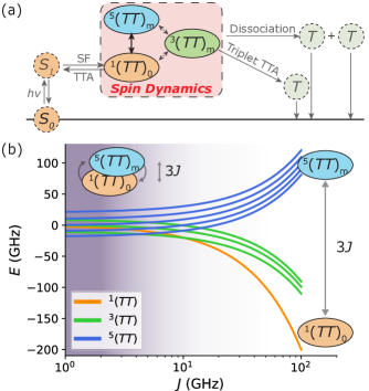
Figure 1: (a) In singlet fission (SF) a singlet exciton decays to an $S=0$ triplet-pair, ${}^{1}(TT)_{0}$, which may dephase to access different spin states ${}^{2S+1}(TT)_{m}~{}(S=0,1,2)$. (b) Energies of triplet pair spin states as a function of exchange coupling $J$.When $J$ is small, spin states are poorly defined and mix freely (shaded area) but at large $J$ spin mixing does not occur.

The spin Hamiltonian for the coupled triplet pair ${}^{2S+1}(TT)_{m}$ can be written as the sum of Zeeman interaction $\hat{H}_{\textrm{Z}}$, zero-field splitting term $\hat{H}_{\textrm{zfs}}$, and intertriplet exchange interaction $\hat{H}_{\textrm{ee}}$ Merrifield, Avakian, and Groff (1969); Merrifield (1971)

$$\hat{H} =\hat{H}_{\textrm{Z}}+\hat{H}_{\textrm{zfs}}+\hat{H}_{\textrm{ee}},$$ (1a)

$$\hat{H}_{\textrm{ee}} =J\hat{S}_{1}\cdot\hat{S}_{2},$$ (1b)

where $J$ is the isotropic exchange integral describing single electron exchange between the two triplet pairs—effectively, a measure of through-bond or through-space contact between the two tripletsKollmar et al. (1982).

Spin dephasing of the ${}^{2S+1}(TT_{m})$ multiexciton is highly sensitive to the magnitude of the $J$ exchange term. Spin mixing to form quintets is only efficient when the exchange term $J$ is small relative to zero field splitting parameter $D$ (1 (b), left),Collins, McCamey, and Tayebjee (2019); Weiss et al. (2017) but the well-resolved ${}^{5}(TT)$ quintets observed in tr-ESR are consistent with a $J$ that is large at the time of measurement (1 (b), right). These seemingly contradictory requirements for $J$ to be both small (for ${}^{5}(TT)_{m}$ formation) and large (consistent with experiment) have led to suggestions that $J$ must fluctuate over timeWeiss et al. (2017); Tayebjee et al. (2017); Nagashima et al. (2018); Collins, McCamey, and Tayebjee (2019); Kobori et al. (2020); Collins et al. (2022), which is supported by recent theoretical works showing the ability of simple $J(t)$ models to drive high quintet yields over experimentally relevant timescales.Collins, McCamey, and Tayebjee (2019); Kobori et al. (2020); Collins et al. (2022)

Building on recent findingsCollins, McCamey, and Tayebjee (2019); Kobori et al. (2020); Collins et al. (2022) that SF quintets can form with abstracted models of $J(t)$, we now extend this approach to calculate SF spin dynamics for molecular materials undergoing molecular dynamics calculated from physical models.

II Methodology

We introduce a modular process for simulating the singlet fission spin dynamics of molecular materials. This model provides an end-to-end pathway from electronic structure calculations to fundamental spin physics, bridging the disciplinary gap between chemistry and spin physics by using molecule-specific properties as input parameters for numerical simulations of spin dynamics. We apply this model to the spin dynamics of a well known pentacene dimer, BP1Trinh et al. (2017)(Fig. 2). BP1 is known to undergo singlet fissionTrinh et al. (2017) and has two principle degrees of internal rotational freedom due to the single (1,4)-phenylene bridge. We anticipate that either of these rotations will modulate $J$ via changes in exciton delocalisation.Collins, McCamey, and Tayebjee (2019); Ringström et al. (2022)

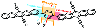
Figure 2: Modelled pentacene dimer BP1. Thermally accessible ring rotations occur about carbon-carbon single bonds and are fully parametrised by a two-dimensional geometry coordinate $\bm{X}(\theta,\phi)$. For real BP1 $\mathrm{R=Si(^{i}Pr)_{3}}$; here $\mathrm{R=H}$ to reduce computational complexity.

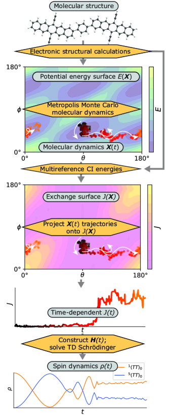
Figure 3: An end-to-end pathway from molecular structure to SF spin dynamics. We model knownTrinh et al. (2017) SF material BP1 over reduced geometry coordinate $\bm{X}(\theta,\phi)$ (Fig. 2). Processes are indicated with yellow boxes and information products are shown in grey lozenges: as the overall schema is modular, the basic procedures used here could easily be replaced with more sophisticated alternatives.

By restricting our analysis to a geometry coordinate $\bm{X}(\theta,\phi)$ containing only the pentacene-pentacene dihedral $\theta$ and pentacene-bridge dihedral $\phi$, the complexity of our calculations can be reduced from an intractable (3N-6) nuclear degrees of freedom to a computationally feasible 2 dimensions.

The schema of the overall model is shown in Fig. 3. First, we use single-reference electronic structural calculations to obtain a potential energy surface (PES) $E(\bm{X})$. We use this PES as the input for a simple Monte Carlo molecular dynamics simulation, generating time-dependent conformation trajectories $\bm{X}(t)$. We then use multireference configuration interaction calculations in a (4e,4o) active spaceSchmidt (2019) to obtain a surface of spin-spin exchange energies, $J(\bm{X})$, and project the previously-obtained molecular dynamics $\bm{X}(t)$ onto this surface to obtain time-dependent exchange trajectories $J(t)$. Finally, the calculated exchange trajectories $J(t)$ are incorporated into the system spin Hamiltonian (Eq. 1a) to obtain spin dynamics of the system as solutions to the time-dependent Schrödinger equation using previously reported methods.Collins, McCamey, and Tayebjee (2019)

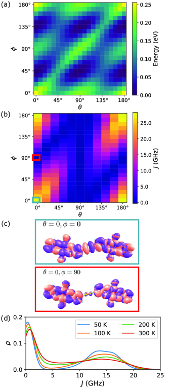
Figure 4: (a) PES for BP1 in the triplet pair $(TT)$ state. (b) The variation of exchange coupling as a function of $\theta$ and $\phi$. Coloured circles indicate where the geometries in (c) lie on the surface. (c) The eight highest energy molecular orbitals with electron density determined by ROHF. The orbitals are rendered for a co-planar geometry (blue) and an orthogonal geometry (red) to illustrate the difference in orbital overlap across the bridge. (d) Probability distribution of exchange $J$ when BP1 is at thermal equilibrium.

III Results

III.1 Potential Energy Surfaces

The ground state PES of BP1 was calculated at the B3LYP Becke (1993)/6-31G(d) Petersson et al. (1988); Petersson and Al‐Laham (1991) level of theory, implemented in Gaussian Frisch et al. (2016). The bulky triisopropyl silane (TIPS) functional groups do not contribute significantly to BP1’s electronic characterKöhler and Bässler (2015) and were substituted with hydrogen atoms to reduce computational complexity, consistent with previous work. Pun et al. (2018) A relaxed potential energy surface scan over a $21\times 21$ point grid spanning $180$ degrees was then completed for the constrained degrees of freedom $\theta$ and $\phi$ (Fig. 2). Due to the symmetry of the molecule, the two $180$ degree scans span the unique energy surface of the configuration space.

The ${}^{2S+1}(TT)_{m}$ triplet pair excited state involves a double excitation and cannot be calculated using standard single reference calculations such as DFT or HF theory Jensen (2007). In contrast, ground states of a given spin multiplicity are straightforward to calculate. We thus approximated the $(TT)$ triplet pair state as equivalent to the lowest energy ($\hat{S}=2$) quintet, allowing us to obtain the excited triplet-pair PES of BP1 with a single-reference relaxed scan across $\theta$ and $\phi$ at the ROHF/6-31G(d) level, drawing on prior work in this areaSchmidt (2019). Figure 4(a) shows the resultant PES for BP1 in the triplet pair state. Approximating the triplet pair state as the ground-state quintet fails to capture the spin-spin interactions that distinguish ${}^{5}(TT)_{m}$ from the other ${}^{M}(TT)_{m}$ states, but the energy scale of these interactions are $\sim 10^{5}$ smaller than the electronic PESTayebjee et al. (2017) and are thus unlikely to influence nuclear conformational dynamics. As the ground and triplet pair states were calculated at different levels of theory (B3LYP and ROHF respectively), direct comparison of the resultant energies is not reasonable. Only the comparative energies within the surfaces are relevant to simulate the dynamics of BP1 and are sufficient for our model.

For both singlet and quintet states, the calculated PES consists of four local minima separated by rotational barriers of $0.1$-$0.3\text{ eV}$. One dimensional slices along the $\theta$ and $\phi$ axes resemble double well potentials with minima located at approximately $35\degree$ and $145\degree$. This is comparable to experimentally determined parameters of biphenylImamura and Hoffmann (1968); Bastiansen and Samdel (1985), a structurally analogous compound, which has an $\approx 0.1\text{ eV}$ barrier to rotation about minima located at approximately $\pm 35\degree$. In the triplet state, the locations of the double well minima are shifted slightly towards planarity and the rotational barrier decreases in height.

III.2 Exchange Coupling

The inter-triplet exchange coupling $J$ was obtained from the energetic separation ($\Delta_{SQ}$) of the singlet and quintet spin states, where $\Delta_{SQ}=3J$ Kollmar et al. (1982); Benk and Sixl (1981). These energies were calculated using a multireference configuration interaction (CI) approach within a (4e,4o) active space, following a methodology previously applied to a model system of ethylene dimersSchmidt (2019). The CI active space was constructed from the four highest-energy orbitals obtained through ROHF/6-31G(d) calculations of the ground-state. Calculations were implemented in the GAMESS program Schmidt et al. (1993), with all determinants considered. Energies of the near-degenerate ${}^{1}(TT)$, ${}^{3}(TT)$, and ${}^{5}(TT)$ spin states were obtained over the $\bm{X}(\theta,\phi)$ coordinate and used to determine the sign and magnitude of $J$. An example output of this calculation can be found in Appendix A.

The coordinate-dependent exchange surface of BP1, $J(\bm{X})$, is shown in Figure 4 (b). Consistent with expectations, $J\simeq 0$ wherever at least one chromophore is orthogonal to the phenyl bridge ($[\phi-\theta]=90\degree,270\degree,\dots$) or where both chromophores are orthogonal ($\theta=90\degree,270\degree,\dots$). The sign of $J$ is almost always positive ($J\geq 0$), meaning that the system shows antiferromagnetic coupling with ${}^{5}(TT)_{0}$ at a higher energy than the ${}^{1}(TT)_{0}$ singlet which differs from some previous reportsRugg et al. (2022); Hasobe et al. (2022). However, there are rare geometries where orthogonal ring orientations result in no orbital overlap and weakly ferromagnetic spin-spin coupling—i.e., where $J\lesssim 0$ (Fig. 4 (c)).

For pentacene dimers such as BP1, the zero field splitting parameter $D$ is on the order of $1$ GHz Tayebjee et al. (2017). As the calculated exchange coupling $J(\bm{X})$ ranges from $J\sim 0$ GHz to $J\sim 30$ GHz, BP1 is able to satisfy the requirement that conformational dynamics must access $J(t)$ values that are sometimes small and sometimes large relative to $D$. This supports the argument that low-energy dynamics on a simple intramolecular coordinate $\bm{X}$ are sufficient to drive spin state mixing via dynamic exchange fluctuations.

The time-averaged occupancy of the exchange surface is determined by thermal Boltzmann statistics of the electronic PES, with $J(t)$ primarily sampling $J(\bm{X})$ values corresponding to local minima of $E(\bm{X})$. Figure 4 (d) shows probability distributions of $J$ weighted by Boltzmann statistics of the underlying $E(\bm{X})$ PES. We find that conformational energy minima $E(\bm{X})$ correspond to $J(\bm{X})$ regions of both large and small $J$ relative to $D$ (Fig. 4 (b)). Intermediate values of $J$ are less populated, supporting the validity of recent workCollins et al. (2022) modelling trajectories through this space as hops between large and small $J$. As temperature increases, the distributions flatten and these intermediate values become more accessible to the molecule although a small bias towards low values of $J$ is retained.

III.3 Metropolis Monte Carlo Simulations

III.3.1 Dynamics of unrestricted BP1

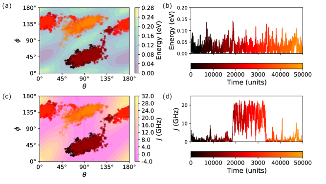
Figure 5: (a) Simulated molecular dynamics $\bm{X}(t)$ obtained by metropolis Monte Carlo evolution over the quintet PES of BP1 at 200 K. (b) Long periods of local exploration within an energy minimum are broken up by infrequent site-hopping over higher-energy saddle points to access adjacent locally-stable conformations. (c) $\bm{X}(t)$ mapped onto the calculated exchange surface $J(\bm{X})$. (d) Transitions between local energy minima produce a noisy step function in exchange space. The colour map indicates the progression of time from the start of the simulation (black) to the end of the simulation (yellow).

The molecular dynamics of BP1 over geometry coordinate $\bm{X}(\theta,\phi)$ were simulated using a Metropolis Monte Carlo algorithm. Simulations were completed as follows (see Appendix B for details): (i) The molecule was initialised in a conformation sampled randomly from the Boltzmann-weighted ground state PES occupancy. (ii) The two dimensional PES of the quintet state (as a surrogate for $(TT)$) was then sampled using a Metropolis-Hastings algorithm modified from prior workTiana, Sutto, and Broglia (2007). (iii) The trajectories produced by the algorithm were mapped onto the exchange surface calculated by CI and used to generate a time dependent value for exchange $J(t)$.

Figure 5 shows a typical trajectory for BP1 at 200 K, demonstrating the ability of this model to capture both low-energy fluctuations around a conformational energy minimum and higher-energy hops between adjacent minima. These molecular dynamics trajectories $\bm{X}(t)$ can then be projected onto the exchange surface $J(\bm{X})$ (Fig. 5 (c)) to obtain a trajectory of dynamics-induced fluctuating exchange, $J(t)$ (d). The exchange fluctuations calculated by this approach appear as noisy step functions: the steps between $J\approx 0$ and $J\approx 15~{}\mathrm{GHz}$ result from rapid transient passage between different locally-stable conformations, while the superimposed noise comes from low-energy dynamics within a conformational energy minimum.

The form of $J(t)$ was found to be robust to changes in the model parameters. The length scale of steps and the maximum individual step-size impact the rate at which transitions occur and the variance in exchange space. However, the core behaviour of a step function between two regimes of $J$ is reproduced.

It is important to note the gas phase PESs calculated in Section III.1 are not ideal analogs for molecules in the condensed phases used for experimental studies of singlet fission (molecular solvents for room-temperature optical measurements, or frozen glasses for low-temperature spin resonance). Nevertheless, these energy landscapes provide a straightforward proof of concept that can be substituted by more accurate models in future iterations of this analytic schema.

III.3.2 Restricting large-amplitude chromophore dynamics

Experimental spin resonance measurements of SF molecular dimers typically occur in frozen solution at cryogenic temperatures or with the molecules held in solid matrices Tayebjee et al. (2017); Sakai et al. (2018); Pun et al. (2019). Whether large changes in geometry can still occur in these systems is not settled Kobori et al. (2020). While the local heating effect of high-energy laser photoexcitation may temporarily allow thermal access to molecular dynamics, large-amplitude dynamics involving bulky chromophore rotations seem unlikely under these circumstances.Concistrè et al. (2014). We thus consider the case of restricted molecular dynamics in which the local environment prevents inter-chromophore rotations of the bulky pentacene groups, freezing $\theta$ such that all dynamics occur on the chromophore-bridge coordinate $\phi$.Illig et al. (2016); Kwon et al. (2015); Nobukawa et al. (2013). Modelling the impact of restricted motion on SF spin dynamics may help inform the types of geometry changes required for SF.

Restricting the $\theta$ degree of freedom only allows transitions between conformations that are accessible via bridge rotations ($\phi$). Figure 6 depicts these allowed transitions in energy and exchange space, showing that the previously-observed step changes in $J$ do not occur in the absence of inter-chromophore rotations. Instead, the trajectories in exchange space are simply thermal fluctuations within the fixed high- or low-$J$ conformation as defined by the initial interchromopore angle $\theta$. In the low exchange regime, $J\sim 0$ GHz, spin states will be able to mix but will never form long-lived states with well defined spin such as those observed in nutation experiments Tayebjee et al. (2017). In contrast, if the molecule is in the large exchange regime $J\sim 15$ GHz, coherent mixing between the singlet and quintet spin states is prohibited. Well-defined $(TT)$ spin states with $S\neq 0$ may still be accessed through other pathways such as stochastic spin-mixing in a high-$J$ manifoldCollins et al. (2022), but these results suggest that acene dimers with a single (1,4-phenylene) bridging motif may have limited pathways for accessing high-spin $(TT)$ states when in restricted environments. Molecules with additional degrees of freedom and multiple conformational minima, such as poly(1,4)-phenylene bridges,Tayebjee et al. (2017) are more likely to enable variation between high- and low-$J$ in restricted geometries.

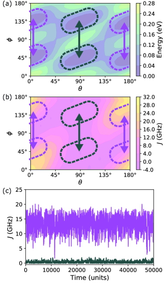
Figure 6: Effect of freezing chromophore-chromophore dynamics $(\theta)$ and only allowing bridge rotations $(\phi)$, as might occur in a solid matrix. (a) Conformational dynamics between locally-stable geometries are still possible, but (b) no longer result in large $J$ changes. (c) Instead, $J(t)$ fluctuates within high-exchange or low-exchange regimes (purple and grey lines, respectively) showing thermal noise without step changes.

III.4 Spin Dynamics

The initial product of SF is a pair of triplet excitons localised on coupled but separate molecular sites. Here we treat the spin Hamiltonian of the triplet pair following the methodology outlined previouslyCollins, McCamey, and Tayebjee (2019); Collins et al. (2022). The Hamiltonian can be written as the sum of the Zeeman interaction ($\hat{H}_{\textrm{Z}}$) from an externally applied magnetic field ($\bm{B}$), the zero-field splitting interactions ($\hat{H}_{\textrm{zfs}}$), and a time-dependent intertriplet exchange interaction ($\hat{H}_{\textrm{ee}}$)

$$\hat{H} = \hat{H}_{\textrm{Z}}+\hat{H}_{\textrm{zfs}}+\hat{H}_{\textrm{ee}},$$ (2a)

$$\hat{H}_{\textrm{Z}} = \mu_{\textrm{B}}g\sum_{i=1,2}\sum_{j=x,y,z}B_{j}\hat{S}_{ij},$$ (2b)

$$\hat{H}_{\textrm{zfs}} = \sum_{i=1,2}\hat{S}_{i}\cdot\bm{D}_{i}\cdot\hat{S}_{i},$$ (2c)

$$\hat{H}_{\textrm{ee}} = J(t)\hat{S}_{1}\cdot\hat{S}_{2},$$ (2d)

where $\mu_{\textrm{B}}$ is the Bohr magneton, $g$ is the Landé g-factor, and $\hat{S}_{i}$ represents the spin operator for the triplet pair on the $i$th chromophore. $\bm{D}_{i}$ is the ZFS tensor of the $i$th chromophore, which is often described by axiality and rhombicity parameters $D$ and $E$ along with an orientation term.

In this work, we apply our simulated Monte Carlo trajectories to obtain a realistic form for $J(t)$ and additionally, incorporate a time dependent ZFS interaction into the model. $J(t)$ is determined directly by the method described above. The time-dependent ZFS interaction was modelled by defining a time-dependent rotation matrix $R_{\textrm{rel}}(\Theta_{1,2})$ that describes the relative inter-triplet orientation of the chromophores over the course of the trajectory. The relative orientation was parameterised by three Euler angles in the $zyz$ convention, $\Theta_{1,2}=(\theta_{z},\theta_{y},\theta_{z}^{\prime})$.

$$\bm{D}_{2} = R_{\textrm{rel}}\bm{D}_{1}R_{\textrm{rel}}^{T},$$ (3)

$$R_{\textrm{rel}} = R_{z}(\theta_{z}^{\prime})R_{y}(\theta_{y})R_{z}(\theta_{z}),$$ (4)

This orientation was approximated by the chromophore-chromophore dihedral $\theta$ over time. As $\theta$ varies, $\bm{D}_{1}$ remains fixed along the $z$-axis while $\bm{D}_{2}$ rotates about the $y$-axis as a function of $R_{\textrm{rel}}(t)=R_{\textrm{rel}}(0,\theta(t),0)$. The parameters of our spin Hamiltonian for BP1 are summarised in Table 1. The time-dependent Schrödinger equation for this system was then solved using the mesolve function in Python quantum toolbox software QuTip Johansson, Nation, and Nori (2012).

Table 1: Parameters used to model the spin Hamiltonian of BP1. Fixed parameters ($g,D,E$ and $\bm{B})$ are from literature.Tayebjee et al. (2017)

Parameter	Value
${g_{x}=g_{y}=g_{z}}$	2.002
${D}$	1138 MHz
${E}$	19 MHz
$\boldsymbol{B}=(B_{x},B_{y},B_{z})$	(0,0,350mT)
$J(t)$	$J(\bm{X}(t))$
$\bm{D}_{i}$	$R_{\textrm{rel}}\bm{D}_{j}R_{\textrm{rel}}^{T}$
$R_{\textrm{rel}}(t)$	$R_{\textrm{rel}}\Bigl{(}0,\theta(t),0\Bigr{)}$

Simulated molecular dynamics trajectories take place over a period of Monte Carlo ‘time’, $t_{\textrm{MC}}$, related to the number of steps taken during the simulation. This $t_{\textrm{MC}}$ time unit is purely a function of the numerical simulation and does not possess physical significance. To model $J(t)$ in physically significant time units, $t_{\textrm{MC}}$ was scaled to a period of real time $t=\alpha t_{\textrm{MC}}$ where $\alpha$ is the timescale parameter. To determine realistic values of $\alpha$, upper and lower bounds for minima transition rates were estimated. With $D\simeq 1$GHz, the oscillation between the ${}^{1}(TT)_{0}$ and ${}^{5}(TT)_{0}$ states when mixed by the ZFS interaction has period $\sim 1$ ns.Collins, McCamey, and Tayebjee (2019) If transitions between $J$ regimes occur much faster than $D$, these processes become decoupled and stochastic $J$-fluctuations are no longer effective at mixing different spin states. Quintets have been observed with coherence times on the order of $\sim 100$ ns at temperatures below $100$ K Weiss et al. (2017); Tayebjee et al. (2017). By assuming quintets rapidly decohere after transitioning to $J\sim 0$ GHz, time spent in the large exchange regime can be considered an upper bound for coherence times. Hence, the average $t_{\textrm{MC}}$ spent in large exchange minima before transitioning was compared and scaled to experimental values of $D$ and coherence times to give a realistic range for $\alpha$ ($\alpha=0.5$ ps to $50$ ps). This approach to scaling Monte Carlo time is sufficient to demonstrate the viability of quintet formation by conformation-induced exchange fluctuations, but cannot provide ab initio predictions of dynamics without scaling. A logical next step beyond the scope of this work would be to replace or re-scale the Monte Carlo trajectories used here with results from molecular dynamics simulations.

III.4.1 Quintet Formation Via Simulated Trajectories

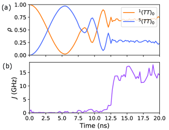
Figure 7: (a) ${}^{1}(TT)_{0}$ and ${}^{5}(TT)_{0}$ projections of the system wavefunction $\psi(t)$ evolving under (b) modelled time-dependent exchange coupling. Initially, the singlet and quintet states mix while $J\simeq 0$. Then, when $J$ quickly becomes too large for the spin states to be mixed by $\hat{H}_{zfs}$, the probability density stabilises.

As in Fig. 5, $J(t)$ dynamics for the unrestricted BP1 dimer appear as a noisy step function between regimes of high and low $J$. Figure 7 shows a numerical solution to the time-dependent Schrödinger equation for a sample $J(t)$ trajectory with $\alpha=3\times 10^{-2}$ ns, demonstrating that these dynamics can lead to well-resolved ${}^{5}(TT)$ quintet multiexcitons. In this trajectory, BP1 is initially in a low-$J$ conformation where ${}^{5}(TT)_{0}$ and ${}^{1}(TT)_{0}$ mix coherently. The system then jumps to a new conformation with $J\approx 15$ GHz, resolving the spin states in energy and freezing mixing with a significant expected population of the $\hat{S}=2$ quintet. Having demonstrated the ability of this model to reproduce quintet formation in a single molecule, we now move to consider the population-averaged spin dynamics of an ensemble of molecules evolving according to this model.

III.4.2 Population Dynamics

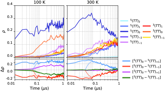
Figure 8: The spin dynamics of an ensemble of 50 BP1 molecules over time at $100$ and $300$ Kelvin. Upper plots depict the population densities while lower plots display the difference in spin populations (spin polarisation). Dotted lines imitate the signal observed by time resolved ESR by filtering the densities with an exponential envelope that rises in at $t=50$ ns to imitate the response time of the experimental apparatus. Rapid formation of the ${}^{5}(TT)_{0}$ quintet occurs for all temperatures with the formation of the ${}^{3}(TT)_{0}$ triplet strongly temperature dependent. The spin densities converge as mixing allows all states other than ${}^{5}(TT)_{2}$ to be populated.

Ensemble simulations of $50$ molecules with motion scaled to $\mathrm{1~{}\mu{}s}$ (details in Appendix C) show spin dynamics qualitatively consistent with experimental observations Tayebjee et al. (2017); Weiss et al. (2017)(Fig. 8). Quintets are populated within $\sim 1$ ns by molecules initialised in $J\sim 0$ GHz minima, allowing immediate spin mixing. At later times, $m_{s}\neq 0$ quintets form more slowly via $\hat{H}_{zfs}$-mediated mixing. As $J_{iso}(t)\geq 0$ and $B>0$, the $m_{s}>0$ ${}^{5}(TT)_{m}$ sublevels remain separated from ${}^{1}(TT)$ by the Zeeman interaction and a bias is seen towards the formation of $m_{s}\leq 0$ spin states. Here the $m_{s}=-1$ quintet is formed preferentially as $J$ is less frequently on resonance with the ${}^{1}(TT)_{0}{}\leftrightarrow{}^{5}(TT)_{-2}$ crossing. These conditions of $B>0$ and $J>0$ also mean that the $m_{s}>0$ quintet states do not easily mix with ${}^{1}(TT)_{0}$ and form slowly. Additionally, the mixing of the triplet with singlet and quintet states is limited by the symmetry of the chromophores Bayliss et al. (2016) and the rate of formation is slow. At low temperatures, where molecules are likely to stay confined to local minima for long periods, the triplet state ${}^{3}(TT)_{0}$ forms with significant polarization from the rest of the triplet manifold.

The formation of polarised spin states is necessarily a transient, kinetic phenomenon: over very long time periods, all spin states are populated and tend towards a near-equal Boltzmann population distribution. Increasing the temperature of the system decreases the time spent in a single local energy minimum and increases the frequency of exchange variations. This inhibits the slow mixing of the ${}^{3}(TT)_{0}$ triplet and increases the number of spin transitions that see a resonant frequency of $J$, and we see less spin polarisation and rapid decay of the initial ${}^{5}(TT)_{0}$ excess at $300$K compared to $100$K. Transitions from the high-$J$ local energy minima to the $J\sim 0$ GHz global minima (Fig. 4(d)) also occur more rapidly at high temperatures, leading to a greater population of ${}^{5}(TT)_{0}$ at early times.

IV Discussion

IV.1 Comparison to Experimental Findings

The results above show that conformation-induced exchange fluctuations in molecular SF dimers can drive spin dynamics and quintet formation. In addition, our simulations suggest that the ${}^{5}(TT)_{\pm 1,2}$ and ${}^{3}(TT)_{0,\pm 1}$ states form with significant initial spin polarisation. The polarisations of these spin states can be probed experimentally with transient electron spin resonance (ESR) spectroscopyTayebjee et al. (2017); Weiss et al. (2017), which measures the $B$-dependent absorption and/or emission of microwaves corresponding to $\Delta m=\pm 1$ spin-spin transitions. Where overlapping transitions exist, resolving the spectra and interpreting the signal can be complex due to the overlap of multiple transitions occurring at the same field. Most relevant to these works, the ${}^{5}(TT)_{\pm 1\leftrightarrow 2}$ and ${}^{3}(TT)_{0\leftrightarrow\pm 1}$ transitions overlap with those of free triplets (${}^{3}T_{0\leftrightarrow\pm 1}$). meaning that the delayed cw-ESR signal previously attributed to free tripletsTayebjee et al. (2017); Weiss et al. (2017) may also have contributions from these spin states. Very recently, ${}^{5}(TT)_{\pm 1\leftrightarrow 2}$ transitions have been experimentally observed for the first time via coherent pulsed ESR (p-ESR)MacDonald et al. (2023), confirming that SF spin dynamics are more complex than first thought.

IV.2 Comparison to Theoretical Models

Proposed models for exchange fluctuation include nuclear reorganisation from small to large exchange regimesCollins, McCamey, and Tayebjee (2019), stochastic switching between two stable regimes (e.g a double potential energy well)Kobori et al. (2020); Collins et al. (2022) and harmonic oscillations within a varying exchange regimeCollins et al. (2022). The quintets formed can be categorised as fast (those that form coherently via ZFS mixing at $J\sim 0$Collins, McCamey, and Tayebjee (2019)), and slow (those that form via stochastic exchange fluctuations at $J>>D$Collins et al. (2022)). The model we present here can inform the validity of each of these theoretical approaches and guide parameter choice for their implementation.

The formation of a fast population of quintets via mixing in a $J\sim 0$ conformation before transitioning to $J>>D$Collins, McCamey, and Tayebjee (2019) is consistent with the PES, exchange surface and simulated dynamics of BP1. These transitions are expected to occur rapidly relative to the time spent in each regime given the high energy of intermediate geometries. Our results are also consistent with a kinetic switching model driven by minima hopping. For these types of exchange fluctuations to occur, it is predicted that large-scale chromophore motions may be required (Section III.3.2).

Recent work has demonstrated that (slow) quintets can be formed when the dimer is confined to a large $J$ regime. Collins et al.Collins et al. (2022) found that diabatic ${}^{1}(TT)_{0}{}\leftrightarrow{}^{5}(TT)_{0}$ transitions can be driven by noise in the exchange signal. When our BP1 model restricts large-scale chromophore motions, a noisy, high $J$ signal, consistent with this approach is observed (Fig. 6 (c)).

Based on this work, we can identify two qualitatively different dynamic regimes, which are likely to lead to two different quintet ensembles, consistent with theoretical modelsCollins, McCamey, and Tayebjee (2019); Collins et al. (2022). The first ensemble, driven by relatively slow dynamical transitions between high and low exchange, forms rapidly ($\sim$ ns) and has short coherence times ($<<\mu$s) whilst the other, fluctuations within a high exchange geometric minima, can lead to stochastic generation of quintets Collins et al. (2022) which take longer to form ($\sim\mu$s), and have longer coherence times ($\sim\mu$s). Relaxation to a $J\sim 0$ minima will allow quintets to decohere by ZFS mixing. As such, the time between minima transitions may provide an upper bound on the coherence time of quintets. Similarly, as the molecule must transition to a $J>>D$ minima for non-stationary quintets to become well defined, the hopping rate places a lower bound on formation time. From this, we see that our BP1 model is consistent either with fast quintets (if minima hops occur with frequency $f\sim$ GHz) or with slow quintets ($f<$ MHz), but not both. Calibrating the timescale of our simulation with short molecular dynamics calculations should help determine which of these mechanisms dominate. The occurrence of both mechanisms simultaneously may be explained by more complex PESs for dimers with additional bridge degrees of freedom. This may allow some dimers to ‘trapped’ within the large $J$ regime while others have the ability to transition between regimes easily. A mixture of molecules in which some have large-scale chromophore motions restricted and/or enabled by solvent interactions may also arise.

IV.3 Implications for Molecular Design

Molecular design is increasingly used to enhance the properties of SF materialsPun et al. (2019); Kobori et al. (2020); Jacobberger et al. (2022). A computational pipeline from molecular structure through to spin dynamics is likely to prove useful as a test-bed for such design. Our results support experimental evidenceNakamura et al. (2021) that more flexible dimers allow quintet states to be formed more rapidly. Rapid population of the quintet manifold prevents decay of the multiexcition via triplet-triplet annihilation and may be beneficial for the quantum yield of SF photovoltaic devicesChen et al. (2019). Decay into low $J$ minima allows quintet spin states to relax and may limit coherence times. Rigid dimers may produce slowly formed, long-lived coherent states that will be beneficial for quantum information applications. The ability to propagate molecular structure data through to simulated spin dynamics could allow novel designs to be developed and suitability assessed.

V Conclusion

We have developed a modular computational pipeline from molecular structure data to physically informed spin dynamics. The model affirms recent observations that the dynamics of the ${}^{1}(TT)_{0}$ state are more complex than models which proceed in a step-wise fashion through the spin manifolds might suggest. The links between the conformational dynamics of the host molecule and evolution of spin states is an important consideration in understanding singlet fission in sufficient detail to design new materials for technological functions. We also show that a number of spin states may contribute to ESR signals previously attributed to free triplets. This methodology informs the validity of existing theoretical approximations for $J(t)$. It’s modular design means it can readily be adapted to other approaches and help determine physically sensible spin simulation parameters. The ability to probe the impact of molecular structure changes on spin dynamics means this pipeline has the potential to form a test bed for molecular design.

Appendix A Determining Exchange

The GAMESS input files for the ROHF and CI calculations are shown in Code Excerpts LABEL:lst:orbs_CI and LABEL:lst:CI_input respectively. The outputs of this calculation were the energies of the lowest 12 $S_{Z}=0$ electronic configurations across the molecular geometry space of the calculations an example of which is shown in Table 2. In this typical output, the lowest three energy states can be identified as the ground singlet state $S_{0}S_{0}$, and the two singly excited triplet states, $\frac{1}{\sqrt{2}}(T_{1}S_{0}+S_{0}T_{1})$ and $\frac{1}{\sqrt{2}}(T_{1}S_{0}-S_{0}T_{1})$, with $\hat{S}=0,1,1$ respectively. The coupled triplet pairs that form the net singlet, triplet and quintet states, ${}^{1}(TT)_{0},^{3}(TT)_{0}$ and ${}^{5}(TT)_{0}$, were then identified as states $4,5$ and $6$. The value for $J$ for a particular geometry was then calculated as the energy difference of state 4 and 6 from GAMESS CI output. The sign of $J$ was determined by whether the $\hat{S}=2$ state was higher or lower (positive or negative $J$) in energy with respect to the $\hat{S}=0$ state.

STATE	ENERGY ($E_{h}$)	SPIN	$\mathbf{S_{z}}$
1	-2213.6207827296	0.00	0.00
2	-2213.6081174362	1.00	0.00
3	-2213.6081009926	1.00	0.00
4	-2213.5954441562	0.00	0.00
5	-2213.5954398750	1.00	0.00
6	-2213.5954313346	2.00	0.00
$\vdots$	$\vdots$	$\vdots$	$\vdots$

Table 2: Example output from the CI calculation

⬇

1#ROHF Calculation to optimize the orbitals for quintet states

2

3 $CONTRL SCFTYP=ROHF RUNTYP=ENERGY

4 MULT=5 ICHARG=0 MAXIT=70

5 $END

6 $DET DISTCI=4 $END

7 $TRANS MPTRAN=2 DIRTRF=.T. AOINTS=DIST $END

8 $MCSCF FULLNR=.F. SOSCF=.T. FOCAS=.F. $END

9 $P2P P2P=.T. DLB=.T. $END

10 $SCF DIIS=.T. SOSCF=.F. $END

11 $SYSTEM TIMLIM=200 MWORDS=200 $END

12 $BASIS GBASIS=N31 NGAUSS=6 NDFUNC=1 $END

13 $GUESS GUESS=HUCKEL $END

14

15 $DATA

16 C58H30

17C1

18CARBON 6.0 -7.682556 -3.647399 0.969669

19CARBON 6.0 -8.027450 -2.518207 0.758059

20. . . . .

21. . . . .

22. . . . .

23HYDROGEN 1.0 1.581654 1.973303 -1.961982

24 $END

Code Excerpt 1: GAMESS input file to determine the orbital occupancy for the quintet state

⬇

1 $SYSTEM TIMLIM=120 MWORDS=500 MEMDDI=8275 $END

2 $CONTRL SCFTYP=NONE RUNTYP=ENERGY

3 MULT=1 ICHARG=0 NOSYM=1

4 CITYP=ALDET

5 $END

6! INTTYP=HONDO ICUT=11 ITOL=30

7 $DET DISTCI=4 $END

8 $TRANS MPTRAN=2 DIRTRF=.T. AOINTS=DIST $END

9 $MCSCF FULLNR=.F. SOSCF=.T. FOCAS=.F. NORB=191 $END

10 $P2P P2P=.T. DLB=.T. $END

11 $SCF DIIS=.T. SOSCF=.F. $END

12 $GUESS GUESS=MOREAD NORB=250 $END

13 $CIDET NCORE=187 NACT=4 NELS=4 NSTATE=12 $END

14

15 $DATA

16 C58H30

17C1 0

18CARBON 6.0 -8.1194440000 3.3501300000 1.5728110000

19 N31 6

20 D 1

21 1 0.8000000000 1.00000000

22.

23.

24.

25 $END

26

27--- OPEN SHELL ORBITALS --- GENERATED AT 12:29:02 12-SEP-2021

28 C58H30

29E(ROHF)= -2213.5581888708, E(NUC)= 5863.4923252874, 17 ITERS

30 $VEC

31 1 1-4.69803246E-09-8.95132119E-09-4.64815196E-09-4.38787828E-09 7.06539514E-10

32 .

33 .

34 .

35 $END

36 POPULATION ANALYSIS

37CARBON 6.53685 -0.53685 6.25662 -0.25662

38. . . . .

39. . . . .

40. . . . .

41HYDROGEN 1.0 1.581654 1.973303 -1.961982

42

43 MOMENTS AT POINT 1 X,Y,Z= -0.000263 0.006091 -0.002655

44 DIPOLE 0.064093 -0.101306 0.075525

Code Excerpt 2: Configuration Interaction Calculation with a (4,4) active space (four electrons constrained to the four highest energy orbitals of the ROHF quintet).

Appendix B Metropolis Monte Carlo Simulations

B.1 Selection of the Metropolis Monte Carlo Method

The pentacene dimer BP1 has two principle degrees of internal rotational freedom about the its single (1,4)-phenylene bridge. The single carbon-carbon bond linking each pentacene chromophore to the phenylene bridge is analogous to the well described internal degree of freedom of biphenylImamura and Hoffmann (1968). Hence, we use the known behaviour of biphenyl to inform our model of BP1 molecular dynamics.

Gas phase biphenyl dynamics are well described by quantised oscillations within and between the potential wells of the biphenyl potential energy surface Chalyavi et al. (2012). Because BP1 singlet fission measurements are in general completed in solution or thin films Tayebjee et al. (2017); Weiss et al. (2017) these oscillations are likely to be rapidly damped by interactions with the solvent Traiphol et al. (2007). Addititionaly, the rotation of the molecule is strongly coupled to the phonon bath of the solution and will proceed in stochastic intra/inter-potential well jumps Banerjee, Yashonath, and Bagchi (2016). Considering the biphenyl energy surfaces and observations of dynamics in solution, we can construct some essential conditions. These conditions are the minimum that must be met to realistically sample from the internal rotational space of BP1 over time.

1. If the system starts in a non equilibrium conformation it will relax back to the energetic minima over some characteristic time.

2. At equilibrium, occupation of energy states will be distributed according to the Boltzmann distribution.

3. The system will stochastically ‘jump’ from one orientation to the next with the transition rate dependent on the energy gap between the two orientations (size of phonon required).

4. Large rotations will be inhibited by the solution and thus rare.

Standard molecular dynamics techniques involve the integration over the equations of motion of the system Mousseau and Barkema (1998). For molecules containing hundreds of atoms, this approach is extremely resource intensive and limits the possible simulation time to $\sim 10^{-9}$ seconds Landau and Binder (2005). Further, the behaviour of molecules in solution is dominated by interactions with the environment  Berkelbach, Hybertsen, and Reichman (2013). This renders the problem more tractable to an open quantum systems approach where the exchange of phonons is explicitly dealt with Breuer and Petruccione (2002); Casanova (2018). The open quantum systems approach requires a degree of complexity in its treatment of the phonon bath that is outside the scope of this paper. Without experimental testing or theoretical modelling of key parameters such as the solution density of states, the assumptions required also limit this approach.

In contrast, the Metropolis algorithm allows for the phonon bath to be treated implicitly Landau and Binder (2005). The algorithm has been used widely to simulate stochastic trajectories and can couple the potential energy landscape to rotation probability, implicitly playing the role of a heat bath Landau and Binder (2005). It can be summarised by the following Metropolis et al. (1953):

1. Choose an initial state $x_{i}$.

2. Wait an amount of time $t_{i}$ distributed around some characteristic time $\tau$. $\tau$ represents the average amount of time between jumps, the time taken to absorb or emit a phonon.

3. Randomly choose a new state to step to $x_{i}^{\prime}=x_{i}+\delta$. The distribution will be problem specific, and likely a free parameter to optimise.

4. Calculate the energy change $\Delta U$ which results from this displacement. If $\Delta U<0$ the move is accepted, $x_{i+1}=x_{i}^{\prime}$. Return to step (2).

5. If $\Delta U>0$, choose a random number $\eta$ uniformly from $0<\eta<1$

6. If $\eta<e^{-\Delta U/k_{B}T}$, accept the move. Here $T$ is the temperature and $k_{B}$ is the Boltzmann constant. Else if $\eta\geq e^{-\Delta U/k_{B}T}$, reject the move and $x_{i+1}=x_{i}$. Return to step (2).

The properties of this algorithm have been extensively studied and it meets many of the requirements outlined above. Firstly, when a system is in equilibrium, the ensemble average of the orientations satisfies the Boltzmann distribution by construction Metropolis et al. (1953). This satisfies requirement (i) and (ii). The method also clearly meets requirement (iii) due to the energy dependencies of step (5) and (6). Work by Tiana et al. has demonstrated that under specific conditions the Metropolis algorithm can reproduce the dynamics of similar stochastic systems Tiana, Sutto, and Broglia (2007), supporting the viability of modelling BP1 in this way.

B.2 Model Implementation

The Metropolis Monte Carlo algorithm was applied to BP1 by linearly interpolating the two dimensional ground and quintet PES’ (Section III.1) into continuous surfaces. With these surfaces obtained, simulations were run as follows:

1. Using the BP1 ground state PES, determine the ground state probability distribution for geometries at input temperature $T$ by calculating the Boltzmann distribution over a $100x100$ square grid. This provides $10000$ initial geometries to choose from with respective probabilities $p_{i}$

   $$p_{i}=\frac{e^{-\epsilon_{i}/K_{B}T}}{\sum_{j=1}^{N}e^{-\epsilon_{j}/K_{B}T}}.$$ (5)

   For a system at thermal equilibrium, Eq. 5 describes the probability ($p_{i}$) the molecule is in the $i$th of $N$ possible conformations at a given timeLandau and Binder (2005). Similarly, $\epsilon_{i}$ and $\epsilon_{J}$ are the energies of the $i$th and $j$th configuration respectively. $K_{B}$ is the Boltzmann constant and $T$ is the temperature of the system.

2. Choose an initial geometry $\bm{X}_{i}(\theta_{i},\phi_{i})$ by drawing from the ground state probability distribution.

   • The selection can be biased to model particular situations. For example, to model the ’freezing in’ of the bulky chromophores by the solvent, the molecule initial conformations can be confined to $\theta_{i}-R<\theta<\theta_{i}+R$.

3. Wait an amount of time $t_{i}$ Lorentz distributed around the characteristic time $\tau$ with scale factor $\gamma_{\tau}$.

4. Randomly choose a new state to step to $\bm{X}_{i}^{\prime}(\theta_{i}^{\prime},\phi_{i}^{\prime})=\bm{X}_{i}(\theta_{i}+\delta\theta,\phi_{i}+\delta\phi)$. This is done by drawing a vector which has orientation uniformly chosen between $0\degree$ and $360\degree$, and which has magnitude drawn from a Lorentz distribution centered on zero with scale factor $\lambda$. The magnitude of the vector cannot be larger than $\delta_{max}$.

5. Using the quintet PES, calculate the energy change $\Delta U$ which results from this displacement. If $\Delta U<0$ the move is accepted, $\bm{X}_{i+1}(\theta_{i+1},\phi_{i+1})=\bm{X}_{i}^{\prime}(\theta_{i}^{\prime},\phi_{i}^{\prime})$. Return to step (2). If the simulation time is greater than $t_{max}$, end the simulation.

6. If $\Delta U>0$, choose a random number $\eta$ uniformly from $0<\eta<1$

7. If $\eta<e^{-\Delta U/k_{B}T}$, accept the move. Here $T$ is the temperature and $k_{B}$ is the Boltzmann constant. Else if $\eta\geq e^{-\Delta U/k_{B}T}$, reject the move and $\theta_{i+1}=\theta_{i}$. Return to step (2). If the simulation time is greater than $t_{max}$, end the simulation.

8. Map the resulting trajectory onto the exchange surface to determine $J$ as a function of Monte Carlo time.

The relevant parameters for this algorithm are described in Table 3. A flowchart of the steps involved is depicted in Fig. 9.

Parameter	Application To Model
$\boldsymbol{T}$	The temperature the simulation is run at. The temperature determines the ground state probability distribution and the Metropolis acceptance ratio $e^{-\Delta U/k_{B}T}$. Thus, the resulting dynamics of the model are strongly dependent on $T$.
$\mathbf{t_{max}}$	The maximum simulation time. This determines how many steps will be taken before the simulation finishes. It should be chosen to ensure that enough Monte Carlo time is simulated for the dynamics of interest (transitions between local minima) to be observed. It is important to note that this is Monte Carlo time and relating this timescale to physical timescales must be done by comparing the simulation behaviour to physical observables or other molecular dynamics models.
$\boldsymbol{\tau}$	The location parameter for the Lorentz distribution of time between steps. $\tau$ represents the time taken to absorb or emit a phonon. This value should be inversely proportional to temperatureTiana, Sutto, and Broglia (2007) ensuring that a hot molecule moves frequently relative to a cold molecule. As only the ratio $\frac{\tau}{t_{max}}$ impacts the dynamics observed, $\tau$ was arbitrarily set to $\frac{100}{T}$ for all simulations. This means that at 100 K the molecule will step on average every 1 unit of time, at 200 K every $\frac{1}{2}$ units of time and so on.
$\boldsymbol{\gamma_{\tau}}$	The scale factor of the Lorentz distribution with location parameter $\tau$ describing time steps.
$\boldsymbol{\lambda}$	The scale factor for the the Lorentz distribution describing the size of steps in configuration space. The distribution is centered on zero and this factor determines the length scale over which the molecule regularly steps (see Fig. 9). This parameter implicitly models the characteristics of the phonon bath and interactions of the molecule with the solution. If $\lambda$ is small, large steps are rare. this means the absorption or release of large phonons required for large changes in geometry are rare.
$\boldsymbol{\delta_{max}}$	The maximum angular distance the molecule is allowed to move in one step. This determines whether large hops across the space are allowed or if the dynamics are constrained to a ’nearest neighbour’ model of traversing the space where only small individual steps are allowed.
$\mathbf{R}$	The restriction parameter. This parameter is used to model the impact of restricting the chromophore-chromophore degree of freedom ($\theta$) to a maximum amplitude of $R\degree$ from the value it was initialised in, only allowing the full rotation of the central bridge ($\phi$). This is a restriction that is expected to occur in frozen solution and will be probed to determine its impact on experimental observables. This is not applicable to the 1D model.

Table 3: The parameters of the Metropolis Monte Carlo model.

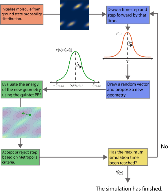
Figure 9: The basic steps of the Metropolis Monte Carlo model.

B.3 Code for Metropolis Monte Carlo simulation

⬇

1#############################################################################

2b1 = np.linspace(AMIN,AMAX,ANUM)

3b2= np.linspace(BMIN,BMAX,BNUM)

4J = interpolate.RectBivariateSpline(b1[:], b2[::2], JDATA[:,::2],kx=1,ky=1)

5E = interpolate.RectBivariateSpline(b1,b2,Q_Es,kx=1,ky=1) # define interpolated energy surface to move on

6G = interpolate.RectBivariateSpline(b1,b2,G_Es) # define ground state energy surface

7#############################################################################

8def find_pop_density(x,y,T):

9 K = 1.380649e-23 #define boltzmann constant

10 sump = 0

11 for a in x:

12 for b in y:

13 sump+= (np.exp(-(G(a,b))/(K*T)))[0][0]

14 G_prob = (np.exp(-(G(x,y))/(K*T))/sump)

15 return G_prob

16

17def find_pop_densityEx(x,y,T):

18 K = 1.380649e-23 #define boltzmann constant

19 sump = 0

20 for a in x:

21 for b in y:

22 sump+= (np.exp(-(E(a,b))/(K*T)))[0][0]

23 E_prob = (np.exp(-(E(x,y))/(K*T))/sump)

24 return E_prob

25

26def prob(E0,E1,T):

27 K = 1.380649e-23

28 return np.exp(-(E1-E0)/(K*T))

29

30def find_nearest(array, value):

31 array = np.asarray(array)

32 idx = (np.abs(array - value)).argmin()

33 return array[idx]

34#############################################################################

35def runsim(deltamax,vi = init ,T = temp, sim_time = tmax, tstep = twidth, runs = N, xw = width, Trajplot = True, trajnum = Nt, densplot=True, Jsurf=True,

36 Jt=True,restricted=[False,None,None]):

37 #Define the 2D mesh

38 x, y = np.linspace(AMIN,AMAX,100), np.linspace(BMIN,BMAX,100)

39 X,Y = np.meshgrid(y,x)

40 theta_grid = [x,y]

41 theta_gridr=[[],[]]

42 theta_grid[0] = theta_grid[0].tolist()

43 theta_grid[1] = theta_grid[1].tolist()

44 gridsize = 180/len(theta_grid[0]) #define the increment between grid points

45 xwidth = xw/gridsize #define average increment to step in grid space by the average distance specified by xw

46 dens = find_pop_density(x,y,T)

47

48 t = 0 #initialise time =0

49 deltat=0

50 K = 1.380649e-23 #define boltzmann constant

51 tau = tstep # set average wait time between steps (was 1e-12sec) now written in nanosec

52 twidth = 0.5 # Distribution varince aroun which tau is centred

53 tlist = [] #setup arrays to store time, angles and change in angles

54 thetas = [[],[]]

55 deltas=[[],[]]

56

57 a = []

58 traj= [] #create a list to store trajectories in

59 l = 0 #initialise tlist length to zero

60 starts=[[],[]]

61 for i in range(0,runs):

62 if vi == ’rand’:

63 xi, yi = random.choice(theta_grid[0]), random.choice(theta_grid[1])

64 x0, y0 = xi, yi

65 starts[0].append(xi)

66 starts[1].append(yi)

67 elif vi == ’mins’:

68 ch = random.choices(dens.ravel(),weights= dens.ravel())

69 coord = np.where(dens==ch)

70 x0,y0 = x[coord[0]],y[coord[1]]

71 starts[0].append(x0)

72 starts[1].append(y0)

73

74 else:

75 x0, y0 = find_nearest(theta_grid[0], vi[0]), find_nearest(theta_grid[1], vi[1]) #map arbitray start points

76

77 #Limit grid according to xlim and ylim in restricted argument

78 if restricted[0] == True and restricted[1]!= None:

79 xmin = x0 - restricted[1]

80 xmax = x0 + restricted[1]

81 if xmax>180:

82 xmax = xmax -180

83 if xmin<0:

84 xmin = xmin +180

85 if restricted[0] == False or restricted[1]== None:

86 xmin = 0

87 xmax = 180

88 if restricted[0] == True and restricted[2]!= None:

89 ymin = y0 - restricted[2]

90 ymax = y0 + restricted[2]

91 if ymax>180:

92 ymax = ymax -180

93 if ymin<0:

94 ymin = ymin +180

95 if restricted[0] == False or restricted[2]== None:

96 ymin = 0

97 ymax = 180

98

99 thetas[0].append(x0)

100 thetas[1].append(y0)

101 tlist.append(0)

102 t = 0

103 c = 0

104 rjct = [[],[]]

105 while t < sim_time:

106 deltat=0

107 while deltat <=0 or deltat>50*tau/T:

108 deltat = stats.cauchy.rvs(loc=tau/T, scale=twidth, size=1)[0]

109 t += deltat #step forward a random amount of time to interact with bath

110 tlist.append(t)

111 E0 = E(x0,y0)

112 J0 = J(x0,y0)

113

114 angle = random.uniform(0, 2.0*np.pi)

115 mag=1000

116 while abs(mag) > deltamax:

117 mag = stats.cauchy.rvs(loc=0, scale=xw, size=1)[0] #

118 #mag = stats.cauchy.rvs(loc=0, scale=xw, size=1)[0]

119 vector = [mag * np.cos(angle), mag * np.sin(angle)] # scaling factor xw

120

121 x1 = x0 +vector[0]

122 y1 = y0 +vector[1]

123

124 #This section updates the index of each angle, evaluates the step size and finally updates the new coordinates

125 #for after the step

126 f=0

127 g=0

128

129 while x1 > 180:

130 x1 = x1 - 180

131 f=1

132 while x1 < 0:

133 x1 = 180 + x1

134 f=2

135

136 if f == 1:

137 delta1 = 180 - abs(x0-x1)

138 elif f== 2:

139 delta1 = -(180 - abs(x0-x1))

140 elif f == 0:

141 delta1 = x0 - x1

142

143 while y1 > 180:

144 y1 = y1 - 180

145 g=1

146 while y1 < 0:

147 y1 = 180 + y1

148 g=2

149

150 if g == 1:

151 delta2 = 180 - abs(y0-y1)

152 elif g== 2:

153 delta2 = -(180 - abs(y0-y1))

154 elif g == 0:

155 delta2 = y0 - y1

156

157 #Here we evaluate the energy of the step and implement the metropolis algorithm

158 E1 = E(x1,y1)

159 if xmin<xmax and xmin>x1 or x1>xmax :

160 E1 = 1000000000

161 if xmin>xmax and x1>xmax and x1<xmin:

162 E1 = 1000000000

163 if ymin<ymax and ymin>y1 or y1>ymax :

164 E1 = 1000000000

165 if ymin>ymax and y1>ymax and y1<ymin:

166 E1 = 1000000000

167 pcut = random.random()

168 if prob(E0,E1,T) > pcut:

169 x0 = x1

170 y0 = y1

171 a.append(1)

172 elif prob(E0,E1,T) <= pcut:

173 delta = 0

174 a.append(0)

175 rjct[0].append(x1)

176 rjct[1].append(y1)

177 thetas[0].append(x0)

178 thetas[1].append(y0)

179 deltas[0].append(delta1)

180 deltas[1].append(delta2)

181

182 if i < trajnum:

183 traj.append([tlist[l:],thetas[0][l:], thetas[1][l:], rjct[0][l:],rjct[1][l:]])

184 l = len(tlist)

185#############################################################################

Code Excerpt 3: Metropolis Monte Carlo simulation for 2-D surfaces

Appendix C Spin Dynamics Calculations

To investigate the ensemble spin dynamics that evolve from Monte Carlo BP1 trajectories, we explored the impact of changes in temperature, hopping rate and chromophore restriction. The simulation length $t_{max}$ was fixed at $20000$ units of Monte Carlo time. This was chosen to allow a number of transitions to occur between local energy minima within each simulation. The full procedure is listed below and the relevant code for the simulation of these dynamics is found in Code Excerpt LABEL:lst:QuTip_model.

1. Generate 50 molecular dynamics trajectories using the Metropolis Monte Carlo model at temperature $T$ and with chromophore restriction $R$. The remaining parameters were fixed according to Table 4.

2. For each trajectory, attain $J(t)$ and $\theta(t)$ by linearly interpolating the values of $J$ and $\theta$ between each time step and scaling the units of time such that $t_{max}=$ Timescale.

3. Solve the time-dependent Schrödinger equation with spin Hamiltonian,

   $$\hat{H}(t)=\hat{H}_{Z}+\hat{H}_{ZFS}(t)+\hat{H}_{EX}(t),$$ (6)

   $$\hat{H}_{Z}=\mu_{B}g\sum_{i=1,2}\sum_{j=x,y,z}B_{j}\hat{S}_{ij},$$ (7)

   $$\hat{H}_{ZFS}(t)=\sum_{i=1,2}\hat{S}_{i}\cdot\mathbf{D_{i}}\left(\theta(t)\right)\cdot\hat{S}_{i},$$ (8)

   $$\hat{H}_{EX}(t)=J(t)\hat{S}_{1}\cdot\hat{S}_{2},$$ (9)

   using the mesolve function of QuTip. The parameters that define this spin Hamiltonian are listed inTable 4. This step is the most computationally expensive. To make the many simulations feasible, the time-dependent functions are only sampled by QuTip at 100 points as the state evolves.

4. Repeat steps (2) and (3) for each timescale in Table 4.

5. Repeat steps (1) through (4) for all combinations of the temperature (T) and restriction (R) parameters in Table 4.

Parameter	Value
${T}$	10, 50, 100, 200, 300, 500 ($\degree K$)
${t_{max}}$	20000
${\tau}$	$\frac{100}{T}$
${\gamma_{\tau}}$	0.5
${\lambda}$	$1\degree$
${\delta_{max}}$	$180\degree$
${R}$	None, $10\degree$

Parameter	Value
${g_{x}=g_{y}=g_{z}}$	2.002
${D}$	1138 MHz
${E}$	19 MHz
$\boldsymbol{B}=(B_{x},B_{y},B_{z})$	(0,0,350mT)
Timescale	10, 100, 1000 (ns)

Table 4: The parameters of the Monte Carlo (left) and spin dynamics (right) simulations.

Resonance Frequency of $J$ (GHz)	Avoided Crossing(s)
$0.00$	${}^{1}(TT)_{0}\sim{{}^{3}(TT)_{0}}\sim{{}^{5}(TT)_{0}}$ ${}^{3}(TT)_{\pm 1}\sim{{}^{5}(TT)_{\pm 1}}$
$3.27$	${}^{1}(TT)_{0}\sim{{}^{5}(TT)_{-1}}$
$4.90$	${}^{3}(TT)_{0}\sim{{}^{5}(TT)_{-1}}$ ${}^{3}(TT)_{+1}\sim{{}^{5}(TT)_{0}}$ ${}^{3}(TT)_{-1}\sim{{}^{5}(TT)_{-2}}$
$6.54$	${}^{1}(TT)_{0}\sim^{5}(TT)_{-2}$
$9.81$	${}^{1}(TT)_{0}\sim{{}^{3}(TT)_{-1}}$ ${}^{3}(TT)_{0}\sim{{}^{5}(TT)_{-2}}$ ${}^{3}(TT)_{+1}\sim{{}^{5}(TT)_{-1}}$
$14.71$	${}^{3}(TT)_{1}\sim{{}^{5}(TT)_{-2}}$

Table 5: The magnitude of $J$ at which the avoided crossings between spin states, denoted by $\sim$, occur.

⬇

1#############################################################################

2#set up the qutip hamiltonians / quantum objects

3#set constants to units of Gz (hence time is in ns)

4g = 2.002

5D_zfs = 1138e-3 #in units of GHz

6E_zfs = 19e-3 #in units of GHz

7B = 350*10**(-3) #in units of Tesla

8mu = scp.physical_constants[’Bohr magneton in Hz/T’][0]*10**(-9) #GHz/T

9#############################################################################

10#Define I of spin-1 hilbert space

11I = qt.qeye(3)

12#define pauli matrices for spin-1 hilbert space

13sx,sy,sz = qt.jmat(1,’x’),qt.jmat(1,’y’),qt.jmat(1,’z’)

14#define spin operators for triplet pair

15sx2 = qt.tensor(sx,I) + qt.tensor(I,sx) # spin projection operators

16sy2 = qt.tensor(sy,I) + qt.tensor(I,sy)

17sz2 = qt.tensor(sz,I) + qt.tensor(I,sz)

18S2 = sx2**2 + sy2**2 + sz2**2 # Total spin S^2

19#############################################################################

20# define our 9 eigenstates of S^2 to project onto

21states = (S2 + sz2).eigenstates()[1]

22psi0 = states[0]

23S0 = states[0]*qt.dag(states[0])

24Tmin1 = states[1]*qt.dag(states[1])

25T0 = states[2]*qt.dag(states[2])

26Tplus1 = states[3]*qt.dag(states[3])

27Qmin2 = states[4]*qt.dag(states[4])

28Qmin1 = states[5]*qt.dag(states[5])

29Q0 = states[6]*qt.dag(states[6])

30Qplus1 = states[7]*qt.dag(states[7])

31Qplus2 = states[8]*qt.dag(states[8])

32#############################################################################

33#Define exchange hamiltonian (sans J(t))

34Hex = (qt.tensor(sz,sz) + qt.tensor(sx,sx) + qt.tensor(sy,sy))

35#define ZFS tensor

36zfst = [[E_zfs-D_zfs/3,0,0],[0,-E_zfs-D_zfs/3,0],[0,0,2*D_zfs/3]] #for molecule along z axis (eul = 0)

37#############################################################################

38#Define the function that takes a MC trajectory and timescale as input and outputs spin densities over #time

39def qutip_evol(trajectory,qutip_time,new_name):

40 #start = time.perf_counter()

41 #Set time grid

42 t= np.linspace(0 ,qutip_time-0.01,100)

43 S0_t = []

44 Q0_t = []

45 #Interpolate J(t) and theta(t)

46 theta_t = interpolate.interp1d(trajectory[0], np.array(trajectory[2]).squeeze()*np.pi/180,kind=’linear’)

47 Js = J.ev(trajectory[1],trajectory[2]).squeeze()

48

49 #smoothing option to reduce cost of noisy signals

50 #N=10000

51 #Jsmooth=uniform_filter1d(Js, size=N)

52 #evaluate = interpolate.interp1d(np.array(trajectory[0]), Jsmooth.squeeze(),kind=’linear’)

53 evaluate = interpolate.interp1d(np.array(trajectory[0]), J.ev(trajectory[1],trajectory[2]).squeeze(),kind=’linear’)

54 #define our function J(t) as the interpolated function

55 def J_t(t,args):

56 return evaluate(t)

57 #Define rotation matrix for relative angle of two chromophores

58 def R_rel(z1,y,z2):

59 Rz1 = np.matrix([[np.cos(z1),-np.sin(z1),0],[np.sin(z1),np.cos(z1),0],[0,0,1]])

60 Ry = np.matrix([[np.cos(y),0,np.sin(y)],[0,1,0],[-np.sin(y),0,np.cos(y)]])

61 Rz2 = np.matrix([[np.cos(z2),-np.sin(z2),0],[np.sin(z2),np.cos(z2),0],[0,0,1]])

62 r = np.matmul(Rz2,Ry,Rz1)

63 return r

64

65 #Define rotation matrix for molecule in relation to B-field

66 def R_B(z1,y,z2):

67 Rz1 = np.matrix([[np.cos(z1),-np.sin(z1),0],[np.sin(z1),np.cos(z1),0],[0,0,1]])

68 Ry = np.matrix([[np.cos(y),0,np.sin(y)],[0,1,0],[-np.sin(y),0,np.cos(y)]])

69 Rz2 = np.matrix([[np.cos(z2),-np.sin(z2),0],[np.sin(z2),np.cos(z2),0],[0,0,1]])

70 r = np.matmul(Rz2,Ry,Rz1)

71 return r

72

73 #define total rotation matrix as combo of both

74 def erot(eul):

75 return np.matmul(R_rel(eul[0],eul[1],eul[2]),R_B(eul[3],eul[4],eul[5]))

76

77 #define time dependent elements of the rotation matrix

78 def R00(t,args):

79 r = np.matmul(np.transpose(erot([0,theta_t(t),0,0,0,0])),np.matmul(zfst,erot([0,theta_t(t),0,0,0,0])))

80 return r[0,0]

81 def R11(t,args):

82 r = np.matmul(np.transpose(erot([0,theta_t(t),0,0,0,0])),np.matmul(zfst,erot([0,theta_t(t),0,0,0,0])))

83 return r[1,1]

84 def R22(t,args):

85 r = np.matmul(np.transpose(erot([0,theta_t(t),0,0,0,0])),np.matmul(zfst,erot([0,theta_t(t),0,0,0,0])))

86 return r[2,2]

87 def R01(t,args):

88 r = np.matmul(np.transpose(erot([0,theta_t(t),0,0,0,0])),np.matmul(zfst,erot([0,theta_t(t),0,0,0,0])))

89 return r[0,1]

90 def R02(t,args):

91 r = np.matmul(np.transpose(erot([0,theta_t(t),0,0,0,0])),np.matmul(zfst,erot([0,theta_t(t),0,0,0,0])))

92 return r[0,2]

93 def R12(t,args):

94 r = np.matmul(np.transpose(erot([0,theta_t(t),0,0,0,0])),np.matmul(zfst,erot([0,theta_t(t),0,0,0,0])))

95 return r[1,2]

96

97 # Construct ZFS hamiltonian with time dependent elements

98 def zfs(zfst,eul):

99 sx,sy,sz = qt.jmat(1,’x’),qt.jmat(1,’y’),qt.jmat(1,’z’)

100 R = np.matmul(np.transpose(erot(eul)),np.matmul(zfst,erot(eul)))

101 H = R[0,0]*(sx**2)+R[1,1]*(sy**2)+R[2,2]*(sz**2)+R[0,1]*(sx*sy+sy*sx)+R[0,2]*(sx*sz+sz*sx)+R[1,2]*(sy*sz+sz*sy)

102 return H

103

104 #Here we have created a time evolving quantum object by making the rotation matrix time dependent

105 #as it stands this only changes the relative orientation of one chromophore and keeps B along z- axis

106 Hzfs1 = qt.QobjEvo([[qt.tensor(sx**2,I), R00], [qt.tensor(sy**2,I),R11], [qt.tensor(sz**2,I),R22],

107 [qt.tensor(sx*sy+sy*sx,I),R01], [qt.tensor(sx*sz+sz*sx,I),R02], [qt.tensor(sy*sz+sz*sy,I),R12]])

108

109 Hzfs = Hzfs1 + qt.tensor(I,zfs(zfst,np.zeros(6))) # we pick one zfs tensor to be our axis and rotate # the other by the relative orientation of the two.

110

111 #define Zeeman hamiltonian

112 Hz = mu*B*g*(qt.tensor(sz,I) + qt.tensor(I,sz))

113 Hz = mu*B*g*(qt.tensor(sz,I) + qt.tensor(I,sz))

114 #Define exchange hamiltonian

115 Hex1 = qt.QobjEvo([[Hex,J_t]])

116

117 #Define total hamiltonian as sum of zeeman, zfs and exhange

118 Ht = Hz + Hzfs + Hex1

119

120 #define time evolved state as a func of time

121 options= qt.Options(nsteps=8000)

122 state_t=qt.mesolve(Ht,psi0,t,options=options).states

123 return t,state_t,theta_t,J_t

Code Excerpt 4: Relevant code for the construction of the Qutip Model