Hypergraph motifs and their extensions beyond binary

Abstract

Hypergraphs naturally represent group interactions, which are omnipresent in many domains: collaborations of researchers, co-purchases of items, and joint interactions of proteins, to name a few. In this work, we propose tools for answering the following questions in a systematic manner: (Q1) what are the structural design principles of real-world hypergraphs? (Q2) how can we compare local structures of hypergraphs of different sizes? (Q3) how can we identify domains from which hypergraphs are?

We first define hypergraph motifs (h-motifs), which describe the overlapping patterns of three connected hyperedges. Then, we define the significance of each h-motif in a hypergraph as its occurrences relative to those in properly randomized hypergraphs. Lastly, we define the characteristic profile (CP) as the vector of the normalized significance of every h-motif. Regarding Q1, we find that h-motifs’ occurrences in $11$ real-world hypergraphs from $5$ domains are clearly distinguished from those of randomized hypergraphs. In addition, we demonstrate that CPs capture local structural patterns unique to each domain, and thus comparing CPs of hypergraphs addresses Q2 and Q3. The concept of CP is naturally extended to represent the connectivity pattern of each node or hyperedge as a vector, which proves useful in node classification and hyperedge prediction.

Our algorithmic contribution is to propose MoCHy, a family of parallel algorithms for counting h-motifs’ occurrences in a hypergraph. We theoretically analyze their speed and accuracy and show empirically that the advanced approximate version MoCHy-A⁺ is up to $25\times$ more accurate and $32\times$ faster than the basic approximate and exact versions, respectively.

Furthermore, we explore ternary hypergraph motifs that extends h-motifs by taking into account not only the presence but also the cardinality of intersections among hyperedges. This extension proves beneficial for all previously mentioned applications.

1 Introduction

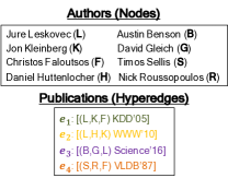
(a) Example data: coauthorship relations

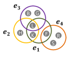
(b) Hypergraph representation

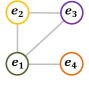
(c) Line-graph representation

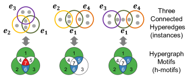
(d) H-motifs and instances

Figure 1: (a) Example: co-authorship relations. (b) Hypergraph: the hypergraph representation of (a). (c) Line Graph: the line-graph representation of (b). (d) Hypergraph Motifs: example h-motifs and their instances in (b).

Complex systems consisting of pairwise interactions between individuals or objects are naturally expressed in the form of graphs. Nodes and edges, which compose a graph, represent individuals (or objects) and their pairwise interactions, respectively. Thanks to their powerful expressiveness, graphs have been used in a wide variety of fields, including social network analysis, web, bioinformatics, and epidemiology. Global structural patterns of real-world graphs, such as power-law degree distribution barabasi1999emergence ; faloutsos1999power and six degrees of separation kang2010radius ; watts1998collective , have been extensively investigated.

In addition to global patterns, real-world graphs exhibit patterns in their local structures, which differentiate graphs in the same domain from random graphs or those in other domains. Local structures are revealed by counting the occurrences of different network motifs milo2004superfamilies ; milo2002network , which describe the patterns of pairwise interactions between a fixed number of connected nodes (typically $3$, $4$, or $5$ nodes). As a fundamental building block, network motifs have played a key role in many analytical and predictive tasks, including community detection benson2016higher ; li2019edmot ; tsourakakis2017scalable ; yin2017local , classification chen2013identification ; lee2019graph ; milo2004superfamilies , and anomaly detection becchetti2010efficient ; shin2020fast .

Despite the prevalence of graphs, interactions in several complex systems are groupwise rather than pairwise: collaborations of researchers, co-purchases of items, joint interactions of proteins, tags attached to the same web post, to name a few. These group interactions cannot be represented by edges in a graph. Suppose three or more researchers coauthor a publication. This co-authorship cannot be represented as a single edge, and creating edges between all pairs of the researchers cannot be distinguished from multiple papers coauthored by subsets of the researchers.

This inherent limitation of graphs is addressed by hypergraphs, which consist of nodes and hyperedges. Each hyperedge is a subset of any number of nodes, and it represents a group interaction among the nodes. For example, the coauthorship relations in Figure 1(a) are naturally represented as the hypergraph in Figure 1(b). In the hypergraph, seminar work leskovec2005graphs coauthored by Jure Leskovec (L), Jon Kleinberg (K), and Christos Faloutsos (F) is expressed as the hyperedge $e_{1}=\{L,K,F\}$, and it is distinguished from three papers coauthored by each pair, which, if they exist, can be represented as three hyperedges $\{K,L\}$, $\{F,L\}$, and $\{F,K\}$.

The successful investigation and discovery of local structural patterns in real-world graphs motivate us to explore local structural patterns in real-world hypergraphs. However, network motifs, which proved to be useful for graphs, are not trivially extended to hypergraphs. Due to the flexibility in the size of hyperedges, it is possible to form $2^{n}$ distinct hyperedges with a given set of $n$ nodes. As a result, the potential number of hypergraphs is $2^{2^{n}}$, which is extraordinarily large even for a small number of nodes. This implies that there can be numerous possible interactions among hyperedges, highlighting the complexity of hypergraph structures.

In this work, taking these challenges into consideration, we define $26$ hypergraph motifs (h-motifs) so that they describe overlapping patterns of three connected hyperedges (rather than nodes). As seen in Figure 1(d), h-motifs describe the overlapping pattern of hyperedges $e_{1}$, $e_{2}$, and $e_{3}$ by the emptiness of seven subsets: $e_{1}\setminus e_{2}\setminus e_{3}$, $e_{2}\setminus e_{3}\setminus e_{1}$, $e_{3}\setminus e_{1}\setminus e_{2}$, $e_{1}\cap e_{2}\setminus e_{3}$, $e_{2}\cap e_{3}\setminus e_{1}$, $e_{3}\cap e_{1}\setminus e_{2}$, and $e_{1}\cap e_{2}\cap e_{3}$. As a result, every overlapping pattern is described by a unique h-motif, independently of the sizes of hyperedges. While this work focuses on overlapping patterns of three hyperedges, h-motifs are easily extended to four or more hyperedges.

We count the number of each h-motif’s instances in $11$ real-world hypergraphs from $5$ different domains. Then, we measure the significance of each h-motif in each hypergraph by comparing the count of its instances in the hypergraph against the counts in properly randomized hypergraphs. Lastly, we compute the characteristic profile (CP) of each hypergraph, defined as the vector of the normalized significance of every h-motif. Comparing the counts and CPs of different hypergraphs leads to the following observations:

• Structural design principles of real-world hypergraphs that are captured by frequencies of different h-motifs are clearly distinguished from those of randomized hypergraphs.

• Hypergraphs from the same domains have similar CPs, while hypergraphs from different domains have distinct CPs (see Figure 2). In other words, CPs successfully capture local structure patterns unique to each domain.

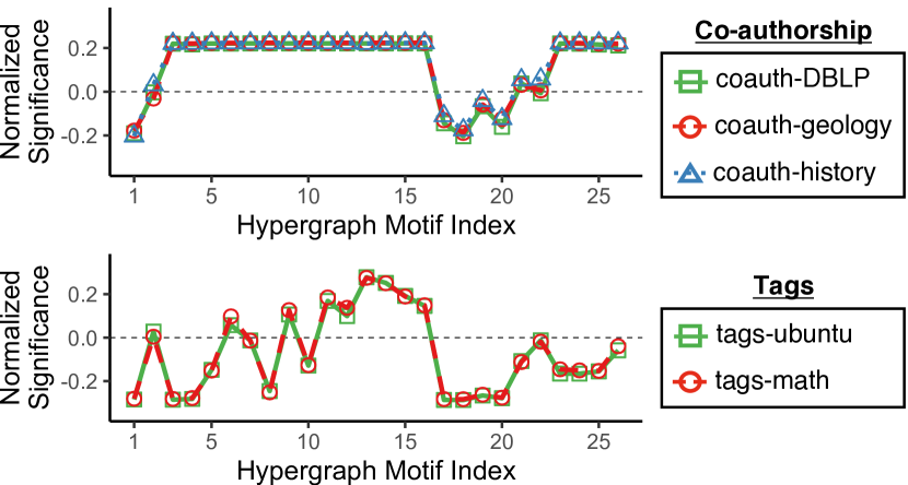
Figure 2: Distributions of h-motifs’ instances precisely characterize local structural patterns of real-world hypergraphs. Note that the hypergraphs from the same domains have similar distributions, while the hypergraphs from different domains do not. See Section 6.3 for details.

Similarly, h-motifs can also be employed to summarize the connectivity pattern of each node or hyperedge. Specifically, for each node, we can calculate its node profile (NP), a 26-element vector with each element indicating the frequency of each motif’s instances within the node’s ego-network. Likewise, the hyperedge profile (HP) of a hyperedge is a 26-element vector with each element representing the count of each motif’s instances that involve the hyperedge. We demonstrate empirically that NPs and HPs effectively capture local connectivity patterns, serving as valuable features for node classification and hyperedge prediction tasks.

Our algorithmic contribution is to design MoCHy (Motif Counting in Hypergraphs), a family of parallel algorithms for counting h-motifs’ instances, which is the computational bottleneck of the aforementioned process. Note that since multi-way overlaps are taken into consideration, counting the instances of h-motifs is more challenging than counting the instances of network motifs, which are defined solely based on pairwise interactions. We provide one exact version, named MoCHy-E, and two approximate versions, named MoCHy-A and MoCHy-A⁺. Empirically, MoCHy-A⁺ is up to $25\times$ more accurate than MoCHy-A, and it is up to $32\times$ faster than MoCHy-E, with little sacrifice of accuracy. These empirical results are consistent with our theoretical analyses.

Additionally, we investigate ternary hypergraph motifs (3h-motifs) as a promising extension of h-motifs. While h-motifs focus only on the emptiness of seven subsets derived from intersections among hyperedges, 3h-motifs further differentiate patterns based on the cardinality of these subsets. In particular, 3h-motifs consider whether the cardinality of each non-empty subset surpasses a specific threshold or not, resulting in $431$ distinct patterns. We demonstrate that employing 3h-motifs instead of h-motifs leads to performance improvements in all the previously mentioned applications, i.e., hypergraph (domain) classification, node classification, and hyperedge prediction.

In summary, our contributions are summarized as follows:

• Novel Concepts: We introduce h-motifs, which capture the local structures of hypergraphs, independently of the sizes of hyperedges or hypergraphs. We extend this concept to 3h-motifs, allowing for a more detailed distinction of local structures.

• Fast and Provable Algorithms: We develop MoCHy, a family of parallel algorithms for counting h-motifs’ instances. We show theoretically and empirically that the advanced version significantly outperforms the basic ones, providing a better trade-off between speed and accuracy.

• Discoveries in $11$ Real-world Hypergraphs: We show that h-motifs and 3h-motifs reveal local structural patterns that are shared by hypergraphs from the same domains but distinguished from those of random hypergraphs and hypergraphs from other domains (see Figure 2).

• Machine Learning Applications: We empirically demonstrate that h-motifs allow for the extraction of effective features in three machine-learning tasks, and employing 3h-motifs enables the extraction of even stronger features.

Reproducibility: The code and datasets used in this work are available at https://github.com/jing9044/MoCHy-with-3h-motif.

This paper is an extension of our previous work lee2020hypergraph , which first introduced the concept of h-motifs and related counting algorithms. In this extended version, we investigate various extensions of h-motifs, including 3h-motifs (Section 5 and Appendices G and H). Furthermore, we develop an advanced on-the-fly algorithm for improved space efficiency (Section 4.4) and establish accuracy guarantees for the approximate counting algorithms in the form of sample concentration bounds (Theorems 4.4 and 4.7). We also evaluate the effectiveness of h-motifs for machine learning applications on three tasks using 7 to 11 datasets (Section 6.5 and Appendices J and K). We especially demonstrate the superior performance of 3h-motifs over their variants and h-motifs in these tasks (Sections 6.4 and 6.5, and Appendix L). Finally, we measure and compare the importance of different h-motifs in characterizing hypergraph structures and their correlation with global structural properties (Section 6.3 and Appendix E).

In Section 2, we introduce h-motifs and related concepts. In Section 3, we describe how we use these concepts to characterize hypergraphs, hyperedges, and nodes. In Section 4, we present exact and approximate algorithms for counting instances of h-motifs, and we analyze their theoretical properties. In Section 5, we extend h-motifs to 3h-motifs. In Section 6, we provide experimental results. After discussing related work in Section 7, we offer conclusions and future research directions in Section 8.

2 Proposed Concepts

Table 1: Frequently-used symbols.

Notation	Definition
$G=(V,E)$	hypergraph with nodes $V$ and hyperedges $E$
$E=\{e_{1},...,e_{|E|}\}$	set of hyperedges
$E_{v}$	set of hyperedges that contains a node $v$
$\wedge$	set of hyperwedges in $G$
$\wedge_{ij}$	hyperwedge consisting of $e_{i}$ and $e_{j}$
$\bar{G}=(E,\wedge,\omega)$	line graph representation of $G$
$\omega(\wedge_{ij})$	the number of nodes shared between $e_{i}$ and $e_{j}$
$N_{e_{i}}$	set of neighbors of $e_{i}$ in $\bar{G}$
$h(\{e_{i},e_{j},e_{k}\})$	h-motif corresponding to an instance $\{e_{i},e_{j},e_{k}\}$
$M[t]$	count of h-motif $t$’s instances

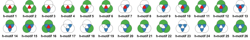
Figure 3: The 26 h-motifs studied in this work. In each Venn diagram, uncolored regions are empty without containing any nodes, while colored regions include at least one node. H-motifs 17 - 22 are open, while the others are closed.

In this section, we introduce preliminary concepts, and based on them, we define the proposed concept, i.e., hypergraph motifs. Refer to Table 1 for the notations frequently used in the paper.

2.1 Preliminaries and Notations

We introduce some preliminary concepts and notations.

Hypergraph: Consider a hypergraph $G=(V,E)$, where $V$ and $E:=\{e_{1},e_{2},...,e_{|E|}\}$ are sets of nodes and hyperedges, respectively. Each hyperedge $e_{i}\in E$ is a non-empty subset of $V$, and we use $|e_{i}|$ to denote the number of nodes in it. For each node $v\in V$, we use $E_{v}:=\{e_{i}\in E:v\in e_{i}\}$ to denote the set of hyperedges that include $v$. We say two hyperedges $e_{i}$ and $e_{j}$ are adjacent if they share any member, i.e., if $e_{i}\cap e_{j}\neq\varnothing$. Then, for each hyperedge $e_{i}$, we denote the set of hyperedges adjacent to $e_{i}$ by $N_{e_{i}}:=\{e_{j}\in E:e_{i}\cap e_{j}\neq\varnothing\}$ and the number of such hyperedges by $|N_{e_{i}}|$. Similarly, we say three hyperedges $e_{i}$, $e_{j}$, and $e_{k}$ are connected if there exists at least one hyperedge among them that is adjacent to the other two.

Hyperwedges: We define a hyperwedge as an unordered pair of adjacent hyperedges. We denote the set of hyperwedges in $G$ by $\wedge:=\{\{e_{i},e_{j}\}\in{E\choose 2}:e_{i}\cap e_{j}\neq\varnothing\}$. We use $\wedge_{ij}\in\wedge$ to denote the hyperwedge consisting of $e_{i}$ and $e_{j}$. In the example hypergraph in Figure 1(b), there are four hyperwedges: $\wedge_{12}$, $\wedge_{13}$, $\wedge_{23}$, and $\wedge_{14}$.

Figure 4: The patterns that cannot be obtained from three distinct hyperedges. For example, any three hyperedges corresponding to the leftmost pattern are necessarily identical. However, according to our definition of hypergraphs in Section 2.1, every hyperedge is unique. Thus, there should be no instance of the pattern.

Line Graph: We define the line graph (a.k.a., projected graph) of a hypergraph $G=(V,E)$ as $\bar{G}=(E,\wedge,\omega)$, where $\wedge$ is the set of hyperwedges and $\omega(\wedge_{ij}):=|e_{i}\cap e_{j}|$. That is, in the line graph $\bar{G}$, hyperedges in $G$ act as nodes, and two of them are adjacent if and only if they share any member. To be more precise, $\bar{G}$ is a weighted variant of a line graph, where each edge is assigned a weight equal to the size of overlap of the corresponding hyperwedge in $G$. Note that for each hyperedge $e_{i}\in E$, $N_{e_{i}}$ is the set of neighbors of $e_{i}$ in $\bar{G}$, and $|N_{e_{i}}|$ is its degree in $\bar{G}$. Figure 1(c) shows the line graph of the example hypergraph in Figure 1(b).

Incidence Graph: We define the incidence graph (a.k.a., star expansion) of a hypergraph $G=(V,E)$ as $G^{\prime}=(V^{\prime},E^{\prime})$ where $V^{\prime}:=V\cup E$ and $E^{\prime}:=\{(v,e)\in V\times E:v\in e\}$. That is, in the bipartite graph $G^{\prime}$, $V$ and $E$ are the two subsets of nodes, and there exists an edge between $v\in V$ and $e\in E$ if and only if $v\in e$.

2.2 Hypergraph Motifs (H-Motifs)

We introduce hypergraph motifs, which are basic building blocks of hypergraphs. Then, we discuss their properties and generalization.

Definition and Representation: Hypergraph motifs (or h-motifs in short) are designed for describing the overlapping patterns of three connected hyperedges. Specifically, given a set $\{e_{i},e_{j},e_{k}\}$ of three connected hyperedges, h-motifs describe its overlapping pattern by the emptiness of the following seven sets: (1) $e_{i}\setminus e_{j}\setminus e_{k}$, (2) $e_{j}\setminus e_{k}\setminus e_{i}$, (3) $e_{k}\setminus e_{i}\setminus e_{j}$, (4) $e_{i}\cap e_{j}\setminus e_{k}$, (5) $e_{j}\cap e_{k}\setminus e_{i}$, (6) $e_{k}\cap e_{i}\setminus e_{j}$, and (7) $e_{i}\cap e_{j}\cap e_{k}$. Formally, a h-motif is defined as a binary vector of size $7$ whose elements represent the emptiness of the above sets, respectively, and as seen in Figure 1(d), h-motifs are naturally represented in the Venn diagram. Equivalently, when we leave at most one node in each of the above subsets, h-motifs can be defined based on the isomorphism between sub-hypergraphs consisting of three connected hyperedges. While there can be $2^{7}$ h-motifs, $26$ h-motifs remain once we exclude symmetric ones, those that cannot be obtained from distinct hyperedges (see Figure 4), and those that cannot be obtained from connected hyperedges. The 26 cases, which we call h-motif 1 through h-motif 26, are visualized in the Venn diagram in Figure 3.

Instances of H-motifs: Consider a hypergraph $G=(V,E)$. A set of three connected hyperedges is an instance of h-motif $t$ if their overlapping pattern corresponds to h-motif $t$. The count of each h-motif’s instances is used to characterize the local structure of $G$, as discussed in the following sections.

Open and Closed H-motifs: A h-motif is closed if all three hyperedges in its instances are adjacent to (i.e., overlapped with) each other. If its instances contain two non-adjacent (i.e., disjoint) hyperedges, a h-motif is open. In Figure 3, h-motifs $17$ - $22$ are open; the others are closed.

Properties of H-motifs: From the definition of h-mot-ifs, the following desirable properties are immediate:

• Exhaustivity: h-motifs capture overlapping patterns of all possible three connected hyperedges.

• Unicity: overlapping pattern of any three connected hyperedges is captured by at most one h-motif.

• Size Independence: h-motifs capture overlapping patterns independently of the sizes of hyperedges. Note that there can be infinitely many combinations of sizes of three connected hyperedges.

Note that the exhaustiveness and the uniqueness imply that overlapping pattern of any three connected hyperedges is captured by exactly one h-motif.

Why Multi-way Overlaps?: Multi-way overlaps (e.g., the emptiness of $e_{1}\cap e_{2}\cap e_{3}$ and $e_{1}\setminus e_{2}\setminus e_{3}$) play a key role in capturing the local structural patterns of real-world hypergraphs. Taking only the pairwise overlaps (e.g., the emptiness of $e_{1}\cap e_{2}$, $e_{1}\setminus e_{2}$, and $e_{2}\setminus e_{1}$) into account limits the number of possible overlapping patterns of three distinct hyperedges to just eight, significantly limiting their expressiveness and thus usefulness. Specifically, $12$ (out of $26$) h-motifs have the same pairwise overlaps, while their occurrences and significances vary substantially in real-world hypergraphs. For example, in Figure 1, $\{e_{1},e_{2},e_{4}\}$ and $\{e_{1},e_{3},e_{4}\}$ have the same pairwise overlaps, while their overlapping patterns are distinguished by h-motifs.

3 Characterization using H-motifs

In this section, we outline the process of using h-motifs to summarize local structural patterns within a hypergraph, as well as those around individual nodes and hyperedges, for the purpose of characterizing them.

3.1 Hypergraph Characterization

What are the structural design principles of real-world hypergraphs distinguished from those of random hypergraphs? Below, we introduce the characteristic profile (CP), which is a tool for answering the above question using h-motifs.

Randomized Hypergraphs: While one might try to characterize the local structure of a hypergraph by absolute counts of each h-motif’s instances in it, some h-motifs may naturally have many instances. Thus, for more accurate characterization, we need random hypergraphs to be compared against real-world hypergraphs. In the network motif literature, configuration models have been widely employed for this purpose milo2004superfamilies ; milo2002network . These models generate random graphs while preserving the degree distribution of the original graph. Using the configuration model does not introduce an excessive level of randomness, maintaining a meaningful and controlled comparison with the original graph.

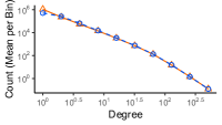
(a) Node: coauth-DBLP

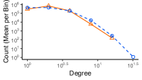
(b) Hyperedge: coauth-DBLP

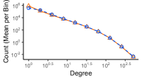
(c) Node: coauth-geology

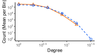
(d) Hyperedge: coauth-geology

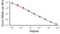
(e) Node: coauth-history

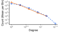
(f) Hyperedge: coauth-history

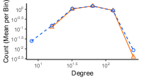
(g) Node: contact-primary

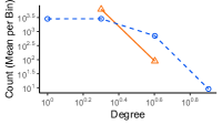
(h) Hyperedge: contact-primary

(i) Node: contact-high

(j) Hyperedge: contact-high

(k) Node: email-Enron

(l) Hyperedge: email-Enron

(m) Node: email-Eu

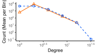
(n) Hyperedge: email-Eu

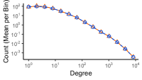
(o) Node: tags-ubuntu

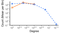
(p) Hyperedge: tags-ubuntu

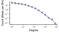
(q) Node: tags-math

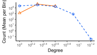
(r) Hyperedge: tags-math

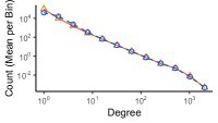
(s) Node: threads-ubuntu

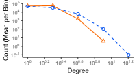
(t) Hyperedge: threads-ubuntu

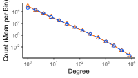
(u) Node: threads-math

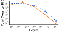
(v) Hyperedge: threads-math

Figure 17: Degree distributions of nodes and size distributions of hyperedges in real-world hypergraphs and the corresponding random hypergraphs.

In line with prior research, we used a configuration model extended to hypergraphs to obtain random hypergraphs. Specifically, we employ the Chung-Lu model aksoy2017measuring , which is a configuration model designed to generate random bipartite graphs while preserving in expectation the degree distributions of the original graph aksoy2017measuring (for a precise theoretical description, please refer to Eq.(20) in Appendix F). We first apply this model to the incidence graph $G^{\prime}$ of the input hypergraph $G$ to obtain randomized bipartite graphs, and then we transform them into random hypergraphs. The empirical distributions of node degrees and hyperedge sizes in the random hypergraphs closely resemble those in $G$, as shown in Figure 17 in Appendix F, where we also provide pseudocode of the process (Algorithm 6) and its theoretical properties.

Significance of H-motifs: We measure the significance of each h-motif in a hypergraph by comparing the count of its instances against the count of them in randomized hypergraphs. Specifically, the significance of a h-motif $t$ in a hypergraph $G$ is defined as

$$\Delta_{t}:=\frac{M[t]-M_{rand}[t]}{M[t]+M_{rand}[t]+\epsilon},\vspace{-1mm}$$ (1)

where $M[t]$ is the number of instances of h-motif $t$ in $G$, and $M_{rand}[t]$ is the average number of instances of h-motif $t$ in randomized hypergraphs. We fixed $\epsilon$ to $1$ throughout this paper. This way of measuring significance was proposed for network motifs milo2004superfamilies as an alternative of normalized Z scores, which can be dominated by few network motifs with small variances. Specifically, when the variance of the occurrences of a specific network motif in randomized graphs is very small, the Z-score becomes significantly large, and thus the Z-score of the particular network motif may dominate all others, regardless of its absolute occurrences.

Characteristic Profile (CP): By normalizing and concatenating the significances of all h-motifs in a hypergraph, we obtain the characteristic profile (CP), which summarizes the local structural pattern of the hypergraph. Specifically, the characteristic profile of a hypergraph $G$ is a vector of size $26$, where each $t$-th element is

$$CP_{t}:=\frac{\Delta_{t}}{\sqrt{\sum_{t=1}^{26}\Delta_{t}^{2}}}.\vspace{-1mm}$$ (2)

Note that, for each $t$, $CP_{t}$ is between $-1$ and $1$. The CP is used in Section 6.3 to compare the local structural patterns of real-world hypergraphs from diverse domains.

3.2 Hyperedge Characterization

Each individual hyperedge can also be characterized by the h-motif instances that contain it.

Hyperedge Profile (HP): Specifically, given a hypergraph $G=(V,E)$, the hyperedge profile (HP) of a hyperedge $e\in E$ is a $26$-element vector, where each $t$-th element is the number of h-motif $t$’s instances that include $e$. It should be noticed that, for HPs, we use absolute counts of h-motif instances rather than their normalized significances. Normalized significances are introduced for CPs to enable direct comparison of hypergraphs at different scales, specifically with varying numbers of nodes and hyperedges. Since comparisons between individual hyperedges, such as for the purpose of hyperedge prediction within a hypergraph, may be free from such issues, we simply use the absolute counts of h-motif instances when defining HPs. In Section 6.5, we demonstrate the effectiveness of HPs as input features in hyperedge prediction tasks.

3.3 Node Characterization

Similarly, we characterize each node by the h-motif instances in its ego network. Below, we introduce three types of ego-networks in hypergraphs, and based on these, we elaborate on the node characterization method.

Hypergraph Ego-networks: Comrie and Kleinberg comrie2021hypergraph defined three distinct types of ego-networks. For each node $v\in V$ in a hypergraph $G=(V,E)$, we denote the neighborhood of $v$ (including $v$ itself) by $V_{v}:=\bigcup_{e_{i}\in E_{v}}e_{i}$, where $E_{v}:=\{e_{i}\in E:v\in e_{i}\}$. The star ego-network of $v$ is a subhypergraph of $G$ with $V_{v}$ as its node set and $E_{v}$ (i.e., the hyperedges that contain $v$) as its hyperedge set. The radial ego-network of $v$ a subhypergraph of $G$ with $V_{v}$ as its node set and $R_{v}:=\{e_{i}\in E:e_{i}\subseteq V_{v}\}$ (i.e., the hyperedges that are subsets of the neighborhood of $v$) as its hyperedge set. Lastly, the contracted ego-network of $v$ has $V_{v}$ as its node set and $C_{v}:=\bigcup_{e_{i}\in E}\{e_{i}\cap V_{v}\}\setminus\emptyset$ as its hyperedge set, and mathematically, the contracted ego-network of $v$ is the subhypergraph of $G$ induced by $V_{v}$. Note that $E_{v}\subseteq R_{v}\subseteq C_{v}$. Compared to $E_{v}$, $R_{v}$ additionally includes hyperedges that consist only of the neighbors of $v$ but not include $v$. Compared to $R_{v}$, $C_{v}$ additionally includes the non-empty intersection of each hyperedge and the neighborhood of $v$.

Node Profile (NP): Given a hypergraph $G=(V,E)$, the node profile (NP) of a node $v\in V$ is a $26$-element where each $t$-th element is the number of h-motif $t$’s instances within an ego-network of $v$. Note that, as for HPs, we use the absolute counts of h-motifs, instead of their normalized significances, for NPs. Depending on the types of ego-networks, we define star node profiles (SNPs), radial node profiles (RNPs), and contracted node profiles (CNPs). In Appendix K, we provide an empirical comparison of these three types of NPs in the context of a node classification task. The results show that using RNPs consistently yields better performance than SNPs or CNPs, indicating that additional complete hyperedges (i.e., $R_{v}\setminus E_{v}$) are helpful, while partial ones extracted from hyperedges (i.e., $C_{v}\setminus R_{v}$) are not.

4 Proposed Algorithms

Given a hypergraph, how can we count the instances of each h-motif? Once we count them in the original and randomized hypergraphs, the significance of each h-motif and the CP are obtained immediately by Eq. (1) and Eq. (2).

In this section, we present MoCHy (Motif Counting in Hypergraphs), which is a family of parallel algorithms for counting the instances of each h-motif in the input hypergraph. We first describe line-graph construction, which is a preprocessing step of every version of MoCHy. Then, we present MoCHy-E, which is for exact counting. After that, we present two different versions of MoCHy-A, which are sampling-based algorithms for approximate counting. Lastly, we discuss parallel and on-the-fly implementations.

Throughout this section, we use $h(\{e_{i},e_{j},e_{k}\})$ to denote the h-motif that describes the connectivity pattern of an h-motif instance $\{e_{i},e_{j},e_{k}\}$. We also use $M[t]$ to denote the count of instances of h-motif $t$.

Input : input hypergraph: $G=(V,E)$

Output : line graph: $\bar{G}=(E,\wedge,\omega)$

$\wedge\leftarrow\varnothing$

3 $\omega\leftarrow$ map whose default value is $0$

4 for each hyperedge $e_{i}\in E$ (in parallel)  do

5       for each node $v\in e_{i}$  do

6             for each hyperedge $e_{j}\in E_{v}$ where $j>i$  do

7                   $\wedge\leftarrow\wedge\cup\{\wedge_{ij}\}$

8                   $\omega(\wedge_{ij})=\omega(\wedge_{ij})+1$

return $\bar{G}=(E,\wedge,\omega)$

(Preprocess)

Algorithm 1 Line Graph Construction

(Preprocess)

Remarks: The problem of counting h-motifs’ occurrences bears some similarity to the classic problem of counting network motifs’ occurrences. However, differently from network motifs, which are defined solely based on pairwise interactions, h-motifs are defined based on triple-wise interactions (e.g., $e_{i}\cap e_{j}\cap e_{k}$). One might hypothesize that our problem can easily be reduced to the problem of counting the occurrences of network motifs, and thus existing solutions (e.g., bressan2019motivo ; pinar2017escape ) are applicable to our problem. In order to examine this possibility, we consider the following two attempts:

1. Represent pairwise relations between hyperedges using the line graph, where each edge $\{e_{i},e_{j}\}$ indicates $e_{i}\cap e_{j}\neq\emptyset$.

2. Represent pairwise relations between hyperedges using the directed line graph where each directed edge $e_{i}\rightarrow e_{j}$ indicates $e_{i}\cap e_{j}\neq\emptyset$ and at the same time $e_{i}\not\subset e_{j}$.

The number of possible connectivity patterns (i.e., network motifs) among three distinct connected hyperedges is just two (i.e., closed and open triangles) and eight in (a) and (b), respectively. In both cases, instances of multiple h-motifs are not distinguished by network motifs, and the occurrences of h-motifs can not be inferred from those of network motifs.

In addition, another computational challenge stems from the fact that triple-wise and even pair-wise relations between hyperedges need to be computed from the input hypergraph, while pairwise relations between edges are given in graphs. This challenge necessitates the precomputation of partial relations, described in the next subsection.

4.1 Line Graph Construction (Algorithm 1)

As a preprocessing step, every version of MoCHy builds the line graph $\bar{G}=(E,\wedge,\omega)$ (see Section 2.1) of the input hypergraph $G=(V,E)$, as described in Algorithm 1. To find the neighbors of each hyperedge $e_{i}$ (line 1), the algorithm visits each hyperedge $e_{j}$ that contains $v$ and satisfies $j>i$ (line 1) for each node $v\in e_{i}$ (line 1). Then for each such $e_{j}$, it adds $\wedge_{ij}=\{e_{i},e_{j}\}$ to $\wedge$ and increments $\omega(\wedge_{ij})$ (lines 1 and 1). The time complexity of this preprocessing step is given in Lemma 1.

Lemma 1 (Complexity of Line Graph Construction).

The expected time complexity of Algorithm 1 is $O(\sum_{\wedge_{ij}\in\wedge}|e_{i}\cap e_{j}|)$.

Proof.

If all sets and maps are implemented using hash tables, the expected time complexity of lines 1 and 1 is $O(1)$ in expectation with uniform hash functions, and they are executed $|e_{i}\cap e_{j}|$ times for each $\wedge_{ij}\in\wedge$. ∎

Since $|\wedge|<\sum_{e_{i}\in E}|{N}_{e_{i}}|$ and $|e_{i}\cap e_{j}|\leq|e_{i}|$, Eq. (3) holds.

$$\sum\nolimits_{\wedge_{ij}\in\wedge}|e_{i}\cap e_{j}|<\sum\nolimits_{e_{i}\in E}(|e_{i}|\cdot|N_{e_{i}}|).$$ (3)

Input :    (1) input hypergraph: $G=(V,E)$

(2) line graph: $\bar{G}=(E,\wedge,\omega)$

Output : exact count of each h-motif $t$’s instances $M[t]$

$M\leftarrow$ map whose default value is $0$

1 for each hyperedge $e_{i}\in E$ (in parallel) do

2       for each unordered hyperedge pair $\{e_{j},e_{k}\}\in$ $N_{e_{i}}\choose 2$ do

3             if $e_{j}\cap e_{k}=\varnothing$ or $i<\min(j,k)$ then

4                   $M[h(\{e_{i},e_{j},e_{k}\})]\mathrel{+}=1$

return $M$

Algorithm 2 MoCHy-E: Exact H-motif Counting

4.2 Exact H-motif Counting (Algorithm 2)

We present MoCHy-E (MoCHy Exact), which counts the instances of each h-motif exactly. The procedures of MoCHy-E are described in Algorithm 2. For each hyperedge $e_{i}\in E$ (line 2), each unordered pair $\{e_{j},e_{k}\}$ of its neighbors, where $\{e_{i},e_{j},e_{k}\}$ is an h-motif instance, is considered (line 2). If $e_{j}\cap e_{k}=\varnothing$ (i.e., if the corresponding h-motif is open), $\{e_{i},e_{j},e_{k}\}$ is considered only once. However, if $e_{j}\cap e_{k}\neq\varnothing$ (i.e., if the corresponding h-motif is closed), $\{e_{i},e_{j},e_{k}\}$ is considered two more times (i.e., when $e_{j}$ is chosen in line 2 and when $e_{k}$ is chosen in line 2). Based on these observations, given an h-motif instance $\{e_{i},e_{j},e_{k}\}$, the corresponding count $M[h(\{e_{i},e_{j},e_{k}\})]$ is incremented (line 2) only if $e_{j}\cap e_{k}=\varnothing$ or $i<\min(j,k)$ (line 2). This guarantees that each instance is counted exactly once. The time complexity of MoCHy-E is given in Theorem 4.1, which uses Lemma 2.

Lemma 2 (Complexity of Computing $h(\{e_{i},e_{j},e_{k}\})$).

Given the input hypergraph $G=(V,E)$ and its line graph $\bar{G}=(E,\wedge,\omega)$, for each h-motif instance $\{e_{i},e_{j},e_{k}\}$, the expected time for computing $h(\{e_{i},e_{j},e_{k}\})$ is $O(\min\\ (|e_{i}|,|e_{j}|,|e_{k}|))$.

Proof.

Assume $|e_{i}|=\min(|e_{i}|,|e_{j}|,|e_{k}|)$, without loss of generality, and all sets and maps are implemented using hash tables. As defined in Section 2.2, $h(\{e_{i},e_{j},e_{k}\})$ is computed in $O(1)$ time from the emptiness of the following sets: (1) $e_{i}\setminus e_{j}\setminus e_{k}$, (2) $e_{j}\setminus e_{k}\setminus e_{i}$, (3) $e_{k}\setminus e_{i}\setminus e_{j}$, (4) $e_{i}\cap e_{j}\setminus e_{k}$, (5) $e_{j}\cap e_{k}\setminus e_{i}$, (6) $e_{k}\cap e_{i}\setminus e_{j}$, and (7) $e_{i}\cap e_{j}\cap e_{k}$. We check their emptiness from their cardinalities. We obtain $e_{i}$, $e_{j}$, and $e_{k}$, which are stored in $G$, and their cardinalities in $O(1)$ time. Similarly, we obtain $|e_{i}\cap e_{j}|$, $|e_{j}\cap e_{k}|$, and $|e_{k}\cap e_{i}|$, which are stored in $\bar{G}$, in $O(1)$ time in expectation with uniform hash functions. Then, we compute $|e_{i}\cap e_{j}\cap e_{k}|$ in $O(|e_{i}|)$ time in expectation by checking for each node in $e_{i}$ whether it is also in both $e_{j}$ and $e_{k}$. From these cardinalities, we obtain the cardinalities of the six other sets in $O(1)$ time as follows:

$$(1)\ |e_{i}\setminus e_{j}\setminus e_{k}|=|e_{i}|-|e_{i}\cap e_{j}|-|e_{k}\cap e_{i}|+|e_{i}\cap e_{j}\cap e_{k}|,$$

$$(2)\ |e_{j}\setminus e_{k}\setminus e_{i}|=|e_{j}|-|e_{i}\cap e_{j}|-|e_{j}\cap e_{k}|+|e_{i}\cap e_{j}\cap e_{k}|,$$

$$(3)\ |e_{k}\setminus e_{i}\setminus e_{j}|=|e_{k}|-|e_{k}\cap e_{i}|-|e_{j}\cap e_{k}|+|e_{i}\cap e_{j}\cap e_{k}|,$$

$$(4)\ |e_{i}\cap e_{j}\setminus e_{k}|=|e_{i}\cap e_{j}|-|e_{i}\cap e_{j}\cap e_{k}|,$$

$$(5)\ |e_{j}\cap e_{k}\setminus e_{i}|=|e_{j}\cap e_{k}|-|e_{i}\cap e_{j}\cap e_{k}|,$$

$$(6)\ |e_{k}\cap e_{i}\setminus e_{j}|=|e_{k}\cap e_{i}|-|e_{i}\cap e_{j}\cap e_{k}|.$$

Hence, the expected time complexity of computing
$h(\{e_{i},e_{j},e_{k}\})$ is $O(|e_{i}|)=O(\min(|e_{i}|,|e_{j}|,|e_{k}|))$. ∎

Theorem 4.1 (Complexity of MoCHy-E).

The expected time complexity of Algorithm 2 is $O(\sum_{e_{i}\in E}(|N_{e_{i}}|^{2}\cdot|e_{i}|))$.

Proof.

Assume all sets and maps are implemented using hash tables. The total number of triples $\{e_{i},e_{j},e_{k}\}$ considered in line 2 is $O(\sum_{e_{i}\in E}|N_{e_{i}}|^{2})$. By Lemma 2, for such a triple $\{e_{i},e_{j},e_{k}\}$, the expected time for computing $h(\{e_{i},e_{j},e_{k}\})$ is $O(|e_{i}|)$. Thus, the total expected time complexity of Algorithm 2 is $O(\sum_{e_{i}\in E}(|e_{i}|\cdot|N_{e_{i}}|^{2}))$, which dominates that of the preprocessing step (see Lemma 1 and Eq. (3)). ∎

Extension of MoCHy-E to H-motif Enumeration:
Since MoCHy-E visits all h-motif instances to count them, it is extended to the problem of enumerating every h-motif instance (with its corresponding h-motif), as described in Algorithm 3. The time complexity remains the same.

Input :    (1) input hypergraph: $G=(V,E)$

(2) line graph: $\bar{G}=(E,\wedge,\omega)$

Output : h-motif instances and their corresponding h-motifs

for each hyperedge $e_{i}\in E$ (in parallel)  do

1       for each unordered hyperedge pair $\{e_{j},e_{k}\}\in$ $N_{e_{i}}\choose 2$ do

2             if $e_{j}\cap e_{k}=\varnothing$ or $i<\min(j,k)$ then

3                   write($e_{i}$, $e_{j}$, $e_{k}$, $h(\{e_{i},e_{j},e_{k}\})$)

Algorithm 3 MoCHy-E_ENUM for H-motif Enumeration

Input :    (1) input hypergraph: $G=(V,E)$

(2) line graph: $\bar{G}=(E,\wedge,\omega)$

(3) number of samples: $s$

Output : estimated count of each h-motif $t$’s instances: $\bar{M}[t]$

$\bar{M}[t]\leftarrow$ map whose default value is $0$

1 for $n\leftarrow 1...s$ (in parallel) do

2       $e_{i}\leftarrow$ sample a uniformly random hyperedge

3       for each hyperedge $e_{j}\in N_{e_{i}}$ do

4             for each hyperedge $e_{k}\in(N_{e_{i}}\cup N_{e_{j}}\setminus\{e_{i},e_{j}\})$ do

5                   if $e_{k}\not\in N_{e_{i}}$ or $j<k$ then

6                         $\bar{M}[h(\{e_{i},e_{j},e_{k}\})]\mathrel{+}=1$

7 for each h-motif $t$ do

8       $\bar{M}[t]\leftarrow\bar{M}[t]\cdot\tfrac{|E|}{3s}$

return $\bar{M}$

Algorithm 4 MoCHy-A: Approximate H-motif Counting Based on Hyperedge Sampling

4.3 Approximate H-motif Counting

We present two different versions of MoCHy-A (MoCHy Approximate), which approximately count the instances of each h-motif. Both versions yield unbiased estimates of the counts by exploring the input hypergraph partially through hyperedge and hyperwedge sampling, respectively.

MoCHy-A: Hyperedge Sampling (Algorithm 4):

MoCHy-A (Algorithm 4) is based on hyperedge sampling. It repeatedly samples $s$ hyperedges from the hyperedge set $E$ uniformly at random with replacement (line 4). For each sampled hyperedge $e_{i}$, the algorithm searches for all h-motif instances that contain $e_{i}$ (lines 4-4), and to this end, the $1$-hop and $2$-hop neighbors of $e_{i}$ in the line graph $\bar{G}$ are explored. After that, for each such instance $\{e_{i},e_{j},e_{k}\}$ of h-motif $t$, the corresponding count $\bar{M}[t]$ is incremented (line 4). Lastly, each estimate $\bar{M}[t]$ is rescaled by multiplying it with $\frac{|E|}{3s}$ (lines 4-4), which is the reciprocal of the expected number of times that each of the h-motif $t$’s instances is counted. This rescaling makes each estimate $\bar{M}[t]$ unbiased, as formalized in Theorem 4.2.

Theorem 4.2 (Bias and Variance of MoCHy-A).

For every h-motif t, Algorithm 4 provides an unbiased estimate $\bar{M}[t]$ of the count $M[t]$ of its instances, i.e.,

$$\mathbb{E}[\bar{M}[t]]=M[t].$$ (4)

The variance of the estimate is

$$\mathbb{V}\mathrm{ar}[\bar{M}[t]]=\frac{1}{3s}\cdot M[t]\cdot(|E|-3)+\frac{1}{9s}\sum_{l=0}^{2}p_{l}[t]\cdot(l|E|-9),$$ (5)

where $p_{l}[t]$ is the number of pairs of h-motif $t$’s instances that share $l$ hyperedges.

Proof.

See Appendix A. ∎

The time complexity of MoCHy-A is given in Theorem 4.3.

Theorem 4.3 (Complexity of MoCHy-A).

The expected time complexity of Algorithm 4 is $O(\frac{s}{|E|}\sum_{e_{i}\in E}(|e_{i}|\cdot|N_{e_{i}}|^{2}))$.

Proof.

Assume all sets and maps are implemented using hash tables. For a sample hyperedge $e_{i}$, computing $N_{e_{i}}\cup N_{e_{j}}$ for every $e_{j}\in N_{e_{i}}$ takes $O(\sum_{e_{j}\in N_{e_{i}}}(|N_{e_{i}}|+|N_{e_{j}}|))$ time in expectation with uniform hash functions if we compute $N_{e_{i}}\cup N_{e_{j}}$ by checking whether each hyperedge $e\in N_{e_{j}}$ is also in $N_{e_{i}}$. By Lemma 2, computing $h(\{e_{i},e_{j},e_{k}\})$ for all considered h-motif instances takes $O(\min(|e_{i}|,|e_{j}|)\cdot\sum_{e_{j}\in N_{e_{i}}}$ $|N_{e_{i}}|+|N_{e_{j}}|)$ time in expectation. Thus, the expected time complexity for processing a sample $e_{i}$ is

$$O(\min(|e_{i}|,|e_{j}|)\cdot\sum\nolimits_{e_{j}\in N_{e_{i}}}(|N_{e_{i}}|+|N_{e_{j}}|))\\ =O(|e_{i}|\cdot|N_{e_{i}}|^{2}+\sum\nolimits_{e_{j}\in N_{e_{i}}}(|e_{j}|\cdot|N_{e_{j}}|)),$$

which can be written as

$$O(\sum\nolimits_{e_{i}\in E}(\mathbb{1}(e_{i}\text{ is sampled})\cdot|e_{i}|\cdot|N_{e_{i}}|^{2})\\ +\sum\nolimits_{e_{j}\in E}(\mathbb{1}(e_{j}\text{ is adjacent to the sample})\cdot|e_{j}|\cdot|N_{e_{j}}|)).$$

From this, linearity of expectation, $\mathbb{E}[\mathbb{1}(e_{i}$ is sampled$)]=\frac{1}{|E|}$, and $\mathbb{E}[\mathbb{1}(e_{j}$ is adjacent to the sample$)]=\frac{|N_{e_{j}}|}{|E|}$, the expected time complexity per sample hyperedge becomes $O(\frac{1}{|E|}$ $\sum_{e_{i}\in E}(|e_{i}|\cdot|N_{e_{i}}|^{2}))$. Hence, the expected total time complexity for processing $s$ samples is
$O(\frac{s}{|E|}\sum_{e_{i}\in E}(|e_{i}|\cdot|N_{e_{i}}|^{2}))$.∎

We also obtain concentration inequalities of MoCHy-A (Theorem 4.4) using Hoeffding’s inequality (Lemma 3), and the inequalities particularly depend on the number of samples and the number of instances of each h-motif.

Lemma 3 (Hoeffding’s Inequality hoeffding1994probability ).

Let $X_{1}$, $X_{2}$, $\dots$, $X_{n}$ be independent random variables with $a_{j}\leq X_{j}\leq b_{j}$ for every $j\in\{1,2,\dots,n\}$. Consider the sum of random variables $X=X_{1}+\dots+X_{n}$, and let $\mu=\mathbb{E}[X]$. Then for any $\tau>0$, we have

$$\Pr[|X-\mu|\geq\tau]\leq 2\exp\left(-\frac{2\tau^{2}}{\sum_{j=1}^{n}(b_{j}-a_{j})^{2}}\right).$$

Theorem 4.4 (Concentration Bound of MoCHy-A).

Let $d_{\max}[t]=\max_{e\in E[t]}|N_{e}|$ where $E[t]:=\bigcup_{h(e_{i},e_{j},e_{j})=t}$ $\{e_{i},e_{j},e_{k}\}$. For any $\epsilon,\delta>0$, if $M[t]>0$ and the number of samples $s>\frac{1}{18\epsilon^{2}}\left(\frac{|E|d_{\max}[t]^{2}}{M[t]}\right)^{2}\log(\frac{2}{\delta})$, then $\Pr(|\bar{M}[t]-M[t]|\geq M[t]\cdot\epsilon)\leq\delta$ holds for each $t\in\{1,2,\dots,26\}$.

Proof.

See Appendix B. ∎

Input :    (1) input hypergraph: $G=(V,E)$

(2) line graph: $\bar{G}=(E,\wedge,\omega)$

(3) number of samples: $r$

Output : estimated count of each h-motif $t$’s instances: $\hat{M}[t]$

$\hat{M}\leftarrow$ map whose default value is $0$

1 for $n\leftarrow 1...r$ (in parallel) do

2       $\wedge_{ij}\leftarrow$ a uniformly random hyperwedge

3       for each hyperedge $e_{k}\in(N_{e_{i}}\cup N_{e_{j}}\setminus\{e_{i},e_{j}\})$ do

4             $\hat{M}[h(\{e_{i},e_{j},e_{k}\})]\mathrel{+}=1$

5      

6for each h-motif $t$ do

7       if 17 $\leq$ t $\leq$ 22 then $\triangleright$ open h-motifs

8             $\hat{M}[t]\leftarrow\hat{M}[t]\cdot\tfrac{|\wedge|}{2r}$

9      else $\triangleright$ closed h-motifs

10             $\hat{M}[t]\leftarrow\hat{M}[t]\cdot\tfrac{|\wedge|}{3r}$

return $\hat{M}$

Algorithm 5 MoCHy-A⁺: Approximate H-motif Counting Based on Hyperwedge Sampling

MoCHy-A⁺: Hyperwedge Sampling (Algorithm 5):

MoCHy-A⁺ (Algorithm 5) provides a better trade-off between speed and accuracy than MoCHy-A. Differently from MoCHy-A, which samples hyperedges, MoCHy-A⁺ is based on hyperwedge sampling. It selects $r$ hyperwedges uniformly at random with replacement (line 5), and for each sampled hyperwedge $\wedge_{ij}\in\wedge$, it searches for all h-motif instances that contain $\wedge_{ij}$ (lines 5-5). To this end, the hyperedges that are adjacent to $e_{i}$ or $e_{j}$ in the line graph $\bar{G}$ are considered (line 5). For each such instance $\{e_{i},e_{j},e_{k}\}$ of h-motif $t$, the corresponding estimate $\hat{M}[t]$ is incremented (line 5). Lastly, each estimate $\hat{M}[t]$ is rescaled so that it unbiasedly estimates $M[t]$, as formalized in Theorem 4.5. To this end, it is multiplied by the reciprocal of the expected number of times that each instance of h-motif $t$ is counted.

Theorem 4.5 (Bias and Variance of MoCHy-A⁺).

For every h-motif t, Algorithm 5 provides an unbiased estimate $\hat{M}[t]$ of the count $M[t]$ of its instances, i.e.,

$$\mathbb{E}[\hat{M}[t]]=M[t].$$ (6)

For every closed h-motif $t$, the variance of the estimate is

$$\mathbb{V}\mathrm{ar}[\hat{M}[t]]=\frac{1}{3r}\cdot M[t]\cdot(|\wedge|-3)+\frac{1}{9r}\sum_{n=0}^{1}q_{n}[t]\cdot(n|\wedge|-9),$$ (7)

where $q_{n}[t]$ is the number of pairs of h-motif $t$’s instances that share $n$ hyperwedges. For every open h-motif $t$, the variance is

$$\mathbb{V}\mathrm{ar}[\hat{M}[t]]=\frac{1}{2r}\cdot M[t]\cdot(|\wedge|-2)+\frac{1}{4r}\sum_{n=0}^{1}q_{n}[t]\cdot(n|\wedge|-4).$$ (8)

Proof.

See Appendix C. ∎

The time complexity of MoCHy-A⁺ is given in Theorem 4.6.

Theorem 4.6 (Complexity of MoCHy-A⁺).

The expected time complexity of Algorithm 5 is $O(\frac{r}{|\wedge|}\sum_{e_{i}\in E}(|e_{i}|\cdot|N_{e_{i}}|^{2}))$.

Proof.

Assume all sets and maps are implemented using hash tables. For a sample hyperwedge $\wedge_{ij}$, computing $N_{e_{i}}\cup N_{e_{j}}$ takes $O(|N_{e_{i}}|+|N_{e_{j}}|)$ time in expectation with uniform hash functions if we compute $N_{e_{i}}\cup N_{e_{j}}$ by checking whether each hyperedge $e\in N_{e_{j}}$ is also in $N_{e_{i}}$. By Lemma 2, computing $h(\{e_{i},e_{j},e_{k}\})$ for all considered h-motif instances takes $O(\min(|e_{i}|,|e_{j}|)\cdot|N_{e_{i}}|+|N_{e_{j}}|)$ time in expectation. Thus, the expected time complexity for processing a sample $\wedge_{ij}$ is $O(\min(|e_{i}|,|e_{j}|)\cdot(|N_{e_{i}}|+|N_{e_{j}}|))=O(|e_{i}|\cdot|N_{e_{i}}|+|e_{j}|\cdot|N_{e_{j}}|),$ which can be written as

$$O(\sum\nolimits_{e_{i}\in E}(\mathbb{1}(e_{i}\text{ is included in the sample})\cdot|e_{i}|\cdot|N_{e_{i}}|)\\ +\sum\nolimits_{e_{j}\in E}(\mathbb{1}(e_{j}\text{ is included in the sample})\cdot|e_{j}|\cdot|N_{e_{j}}|)).$$

From this, linearity of expectation, $\mathbb{E}[\mathbb{1}(e_{i}$ is included in the sample$)]=\frac{|N_{e_{i}}|}{|\wedge|}$, and $\mathbb{E}[\mathbb{1}(e_{j}$ is included in the sample$)]=\frac{|N_{e_{j}}|}{|\wedge|}$, the expected time complexity per sample hyperwedge is $O(\frac{1}{|\wedge|}\sum_{e_{i}\in E}(|e_{i}|\cdot|N_{e_{i}}|^{2}))$. Hence, the total time complexity for processing $r$ samples is $O(\frac{r}{|\wedge|}\sum_{e_{i}\in E}(|e_{i}|\cdot|N_{e_{i}}|^{2}))$.∎

Additionally, we derive concentration inequalities for MoCHy-A⁺ (Theorem 4.7), following a similar approach to that of Theorem 4.4, but with different minimum sample sizes for guaranteeing the same bound.

Theorem 4.7 (Concentration Bound of MoCHy-A⁺).

Let $d_{\max}[t]=\max_{e\in E_{[t]}}|N_{e}|$ where $E[t]:=\bigcup_{h(e_{i},e_{j},e_{j})=t}$ $\{e_{i},e_{j},e_{k}\}$. For each $t\in\{1,\dots,26\}$ such that $M[t]>0$ and for any $\epsilon,\delta>0$, a sufficient condition of being $\Pr(|\hat{M}[t]-M[t]|\geq M[t]\cdot\epsilon)\leq\delta$ is $r>\frac{1}{18\epsilon^{2}}\left(\frac{|\Lambda|d_{\max}[t]}{M[t]}\right)^{2}$ $\log(\frac{2}{\delta})$, if h-motif $t$ is closed, and $r>\frac{1}{8\epsilon^{2}}\left(\frac{|\Lambda|d_{\max}[t]}{M[t]}\right)^{2}$ $\log(\frac{2}{\delta})$, if motif $t$ is open.

Proof.

See Appendix D. ∎

Comparison of MoCHy-A and MoCHy-A⁺: Empirically, MoCHy-A⁺ provides a better trade-off between speed and accuracy than MoCHy-A, as presented in Section 6.7. We provide an analysis that supports this observation. Assume that the numbers of samples in both algorithms are set so that $\alpha=\frac{s}{|E|}=\frac{r}{|\wedge|}$. For each h-motif $t$, since both estimates $\bar{M}[t]$ of MoCHy-A and $\hat{M}[t]$ of MoCHy-A⁺ are unbiased (see Eqs. (4) and (6)), we only need to compare their variances. By Eq. (5), $\mathbb{V}\mathrm{ar}[\bar{M}[t]]=O(\frac{M[t]+p_{1}[t]+p_{2}[t]}{\alpha})$, and by Eq. (7) and Eq. (8), $\mathbb{V}\mathrm{ar}[\hat{M}[t]]=O(\frac{M[t]+q_{1}[t]}{\alpha})$. By definition, $q_{1}[t]\leq p_{2}[t]$, and thus $\frac{M[t]+q_{1}[t]}{\alpha}\leq\frac{M[t]+p_{1}[t]+p_{2}[t]}{\alpha}$. Moreover, in real-world hypergraphs, $p_{1}[t]$ tends to be several orders of magnitude larger than the other terms (i.e., $p_{2}[t]$, $q_{1}[t]$, and $M[t]$), and thus $\bar{M}[t]$ of MoCHy-A tends to have larger variance (and thus larger estimation error) than $\hat{M}[t]$ of MoCHy-A⁺. Despite this fact, as shown in Theorems 4.3 and 4.6, MoCHy-A and MoCHy-A⁺ have the same time complexity, $O(\alpha\cdot\sum_{e_{i}\in E}(|e_{i}|\cdot|N_{e_{i}}|^{2}))$. Hence, MoCHy-A⁺ is expected to give a better trade-off between speed and accuracy than MoCHy-A, as confirmed empirically in Section 6.7.

Regarding the concentration lower bounds of the number of samples (Theorems 4.4 and 4.7), the ratio of the bound in MoCHy-A to that MoCHy-A⁺ is $\frac{|E|\cdot d_{\max}[t]}{|\wedge|}$ for each closed h-motif $t$, and $\frac{4|E|\cdot d_{\max}[t]}{9|\wedge|}$ for each open h-motif $t$. In real-world datasets (refer to Table 2 in Section 6.1), the maximum value (across all h-motifs) of $\frac{|E|\cdot d_{\max}[t]}{|\wedge|}$ varies from $5$ (in the contact-primary) to $500$ (in the coauth-history). That is, MoCHy-A⁺ requires fewer samples than MoCHy-A for the same bound, thereby supporting the empirical superiority of MoCHy-A⁺ over MoCHy-A. However, it is important to note a limitation in this comparison of bounds. Our concentration bounds may not be optimal since they are based on worst-case scenarios, relying on the term $d_{\max}[t]$.

4.4 Parallel and On-the-fly Implementations

We discuss parallelization of MoCHy and then on-the-fly computation of line graphs.

Parallelization: All versions of MoCHy and line-graph construction are easily parallelized as highlighted in Algorithms 1-5. Specifically, we can parallelize line-graph construction and MoCHy-E by letting multiple threads process different hyperedges (in line 1 of Algorithm 1 and line 2 of Algorithm 2) independently in parallel. Similarly, we can parallelize MoCHy-A and MoCHy-A⁺ by letting multiple threads sample and process different hyperedges (in line 4 of Algorithm 4) and hyperwedges (in line 5 of Algorithm 5) independently in parallel. The estimated counts of the same h-motif obtained by different threads are summed up only once before they are returned as outputs. We present some empirical results in Section 6.7.

H-motif Counting without Line Graphs: If the input hypergraph $G$ is large, computing its line graph $\bar{G}$ (Algorithm 1) is time and space-consuming. Specifically, building $\bar{G}$ takes $O(\sum_{\wedge_{ij}\in\wedge}|e_{i}\cap e_{j}|)$ time (see Lemma 1) and requires $O(|E|+|\wedge|)$ space, which often exceeds $O(\sum_{e_{i}\in E}$ $|e_{i}|)$ space required for storing $G$. Thus, instead of precomputing $\bar{G}$ entirely, we can build it incrementally while memoizing partial results within a given memory budget. We apply this idea to MoCHy-A⁺, resulting in the following two versions of the algorithm:

• On-the-fly MoCHy-A⁺ (Basic): This is a strightfoward application of the memoization idea to MoCHy-A⁺ (Algorithm 5). We compute the neighborhood of a hyperedge $e_{i}\in E$ in $\bar{G}$ (i.e., $\{(k,\omega(\wedge_{ik})):k\in N_{e_{i}}\}$) only if (1) a hyperwedge with $e_{i}$ (e.g., $\wedge_{ij}$) is sampled (in line 5) and (2) its neighborhood is not memoized. The computed neighborhood is memoized with priority based on the degree $|N_{e_{i}}|$ of $e_{i}$ in $\bar{G}$. That is, if the memoization budget is exceeded, we evict the memoized neighborhood of hyperedges in decreasing order of their degrees in $\bar{G}$ until the budget is met. This is because the neighborhood of high-degree hyperedges is frequently retrieved, despite a higher computational cost. According to our preliminary studies, this memoization scheme based on degree demonstrates faster speeds compared to memoizing the neighborhood of random hyperedges or least recently used (LRU) hyperedges.

• On-the-fly MoCHy-A⁺ (Adv.): This is an improved version that considers the order in which hyperwedges are processed. It first collects a list $W$ of sampled hyperwedges and groups the hyperwedges consisting of the same hyperedge. Between the two hyperedges forming a hyperwedge, the one with the larger neighborhood is used to group the hyperwedge. The hyperwedges are processed group by group, and thus hyperwedges consisting of the same hyperedges are more likely to be processed consecutively, thereby increasing the chance of utilizing memoized neighborhoods before they are evicted. As a result, On-the-fly MoCHy-A⁺ (Adv.) is empirically faster than On-the-fly MoCHy-A⁺ (Basic), as shown in Section 6.7.

For details of On-the-fly MoCHy-A⁺ (Basic) and On-the-fly MoCHy-A⁺ (Adv.), refer to Algorithms 8 and 9, respectively, in Appendix I.

5 Extensions of H-motifs

In this section, we explore two distinct approaches to extending the concept of h-motifs. We especially define ternary hypergraph motifs, which demonstrate consistent advantages for a variety of real-world applications.

5.1 Extensions Beyond Binary

As defined in Section 2.2, h-motifs describe overlapping patterns of three hyperedges solely based on the emptiness of the seven subsets derived from their intersections. That is, for each subset, h-motifs classify it into binary states, non-empty or empty, which corresponds to being colored or uncolored in Figure 3. This coarse classification inevitably results in the loss of detailed information within the intersections. Below, we introduce ternary hypergraph motifs, which mitigate this information loss by assigning ternary states to each subset based on its cardinality.

Definition of 3H-motifs: Ternary hypergraph motifs (or 3h-motifs in short) are the extension of h-motifs, so as h-motifs are, they are designed for describing the overlapping pattern of three connected hyperedges. Given an instance (i.e., three connected hyperedges) $\{e_{i},e_{j},e_{k}\}$, 3h-motifs describe its overlapping pattern by the cardinality of the following seven sets: (1) $e_{i}\setminus e_{j}\setminus e_{k}$, (2) $e_{j}\setminus e_{k}\setminus e_{i}$, (3) $e_{k}\setminus e_{i}\setminus e_{j}$, (4) $e_{i}\cap e_{j}\setminus e_{k}$, (5) $e_{j}\cap e_{k}\setminus e_{i}$, (6) $e_{k}\cap e_{i}\setminus e_{j}$, and (7) $e_{i}\cap e_{j}\cap e_{k}$. Differently from h-motifs, which consider two states for each subset (empty or non-empty), 3h-motifs takes into account three (denoted by the ‘3’ in 3h-motifs.) states for each subset. Specifically, for each of these seven sets, we classify it into three states based on its cardinality $c$ as follows: (1) $c=0$, (2) $0<c\leq\theta$, (3) $c>\theta$, where $\theta\geq 1$. Throughout this paper, we set the value of $\theta$ to $1$, and thus each of these seven sets is classified into one of three categories: empty, singleton, and multiple. Equivalently, if we leave $\min(\lceil c/\theta\rceil,2)$ node in each of the above subsets with cardinality $c$, 3h-motifs can be defined based on the isomorphism between sub-hypergraphs formed by three connected hyperedges. Refer to Appendix L for a discussion on 3h-motifs with different values of $\theta$ and additional variants of 3h-motifs. Out of the $3^{7}$ possible patterns, $431$ 3h-motifs remain if we exclude symmetric ones, those that cannot be obtained from distinct hyperedges, and those that cannot be derived from connected hyperedges. Visual representations of 3h-motifs 1-6, which are the six 3h-motifs subdivided from h-motif 1, are provided in Figure 5. For a complete list of all 431 3h-motifs, refer to Appendix L.

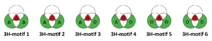
Figure 5: The six 3h-motifs subdivided from h-motif 1. In each Venn diagram, uncolored regions are empty without containing any nodes. Colored regions with a triangle contain more than 0 and at most $\theta$ nodes, while colored regions with a circle contain more than $\theta$ nodes. Throughout this paper, we set $\theta$ to $1$.

Characterization using 3H-motifs: 3H-motifs can naturally substitute h-motifs for characterizing hypergraphs, hyperedges, and nodes. By using 3h-motifs, characteristic profiles (CPs), hyperedge profiles (HPs), and node profiles (NPs) become $431$-element vectors.

Counting 3H-motifs’ Instances: To count instances of 3h-motifs using the MoCHy, the only necessary change is to replace $h(\{e_{i},e_{j},e_{k}\})$ with $h_{3}(\{e_{i},e_{j},e_{k}\})$, which provides the corresponding 3h-motif for a given instance $\{e_{i},e_{j},e_{k}\}$. As formalized in Lemma 4, $h_{3}(\{e_{i},e_{j},e_{k}\})$ can be computed with the same time complexity as $h(\{e_{i},e_{j},e_{k}\})$, and thus replacing $h(\{e_{i},e_{j},e_{k}\})$ with $h_{3}(\{e_{i},e_{j},e_{k}\})$ does not change the time complexity of all versions of MoCHy.

Lemma 4 (Complexity of Computing $h_{3}(\{e_{i},e_{j},e_{k}\})$).

Given the input hypergraph $G=(V,E)$ and its line graph $\bar{G}=(E,\wedge,\omega)$, for each 3h-motif instance $\{e_{i},e_{j},e_{k}\}$, the expected time complexity for computing $h_{3}(\{e_{i},e_{j},e_{k}\})$ is $O(\min(|e_{i}|,|e_{j}|,|e_{k}|))$.

Proof.

Following the proof of Lemma 2, we can show that it takes $O(\min(|e_{i}|,|e_{j}|,|e_{k}|))$ time in expectation to obtain the cardinalities of all the following sets: (1) $e_{i}\setminus e_{j}\setminus e_{k}$, (2) $e_{j}\setminus e_{k}\setminus e_{i}$, (3) $e_{k}\setminus e_{i}\setminus e_{j}$, (4) $e_{i}\cap e_{j}\setminus e_{k}$, (5) $e_{j}\cap e_{k}\setminus e_{i}$, (6) $e_{k}\cap e_{i}\setminus e_{j}$, and (7) $e_{i}\cap e_{j}\cap e_{k}$. Based on the cardinality $c$ of each of the seven sets, it takes $O(1)$ time to classify it into (1) $c=0$, (2) $0<c\leq\theta$, and (3) $c>\theta$. Classifying all seven sets, which takes $O(1)$ time, determines a specific 3h-motif. Thus, the expected time complexity of computing $h_{3}(\{e_{i},e_{j},e_{k}\})$ is $O(\min(|e_{i}|,|e_{j}|,|e_{k}|))$, which is same as that of computing $h(\{e_{i},e_{j},e_{k}\})$. ∎

Extensions Beyond Ternary: The concept of 3h-motifs can be generalized to $k$h-motifs for any $k>3$ by classifying each of the seven considered sets into $k$ states. For instance, for $k=4$, each set can be classified into four states based on its cardinality $c$ as follows: (1) $c=0$, (2) $0<c\leq\theta_{1}$, (3) $\theta_{1}<c\leq\theta_{2}$, (4) $c>\theta_{2}$, where $\theta_{2}>\theta_{1}\geq 1$. The number of $k$h-motifs increases rapidly with respect to $k$. Specifically, the number becomes $3,076$ for $k=4$, $14,190$ for $k=5$, and $49,750$ for $k=6$, as derived in Appendix H. In this study, we concentrate on h-motifs and 3h-motifs (i.e., $k=2$ and $k=3$), which are already capable of characterizing local structures in real-world hypergraphs, as evidenced by the empirical results in Section 6.

5.2 Extensions Beyond Three Hyperedges

The concept of h-motifs is easily generalized to four or more hyperedges. For example, a h-motif for four hyperedges can be defined as a binary vector of size $15$ indicating the emptiness of each region in the Venn diagram for four sets. After excluding disconnected ones, symmetric ones, and those that cannot be obtained from distinct hyperedges, there remain $1,853$ and $18,656,322$ h-motifs for four and five hyperedges, respectively, as discussed in detail in Appendix G. This work focuses on the h-motifs for three hyperedges, which are already capable of characterizing local structures of real-world hypergraphs, as shown empirically in Section 6.

6 Experiments

Table 2: Statistics of 11 real hypergraphs from 5 domains.

Dataset	$|V|$	$|E|$	$|\bar{e}|$*	$|\wedge|$	$|\bar{N_{e}}|$**	# H-motifs
coauth-DBLP	1,924,991	2,466,792	25	125M	3,016	26.3B $\pm$ 18M
coauth-geology	1,256,385	1,203,895	25	37.6M	1,935	6B $\pm$ 4.8M
coauth-history	1,014,734	895,439	25	1.7M	855	83.2M
contact-primary	242	12,704	5	2.2M	916	617M
contact-high	327	7,818	5	593K	439	69.7M
email-Enron	143	1,512	18	87.8K	590	9.6M
email-EU	998	25,027	25	8.3M	6,152	7B
tags-ubuntu	3,029	147,222	5	564M	40,836	4.3T $\pm$ 1.5B
tags-math	1,629	170,476	5	913M	49,559	9.2T $\pm$ 3.2B
threads-ubuntu	125,602	166,999	14	21.6M	5,968	11.4B
threads-math	176,445	595,749	21	647M	39,019	2.2T $\pm$ 883M
$*$ The maximum size of a hyperedge. $**$ The maximum degree in the line graph.

Table 3: Real-world and random hypergraphs have distinct distributions of h-motif instances. We report the absolute counts of each h-motif’s instances in a real-world hypergraph from each domain and its corresponding random hypergraph. To compare the counts in both hypergraphs, we measure the relative count (RC) of each h-motif. We also rank the counts, and we report each h-motif’s rank difference (RD) in the real-world and corresponding random hypergraphs.

In this section, we review the experiments that we design for answering the following questions:

• Q1. Comparison with Random: Does counting instances of different h-motifs reveal structural design principles of real-world hypergraphs distinguished from those of random hypergraphs?

• Q2. Comparison across Domains: Do characteristic profiles capture local structural patterns of hypergraphs unique to each domain?

• Q3. Comparison of Characterization Powers: How well do h-motifs, 3h-motifs, and network motifs capture the structural properties of real-world hypergraphs?

• Q4. Machine Learning Applications: Can h-motifs and 3h-motifs offer useful input features for machine learning applications?

• Q5. Further Discoveries: What interesting discoveries can be uncovered by employing h-motifs in real-world hypergraphs?

• Q6. Performance of Counting Algorithms: How fast and accurate are the different versions of MoCHy?

6.1 Experimental Settings

Machines: We conducted all the experiments on a machine with an AMD Ryzen 9 3900X CPU and 128GB RAM.

Implementations: We implemented every version of MoCHy using C++ and OpenMP. For hash tables, we used the implementation named ‘unordered_map’ provided by the C++ Standard Template Library.

Datasets: We used the following eleven real-world hypergraphs from five different domains:

• co-authorship (coauth-DBLP, coauth-geology sinha2015overview , and coauth-history sinha2015overview ): A node represents an author. A hyperedge represents all authors of a publication.

• contact (contact-primary stehle2011high and contact-high mastrandrea2015contact ): A node represents a person. A hyperedge represents a group interaction among individuals.

• email (email-Enron klimt2004enron and email-EU leskovec2005graphs ; yin2017local ): A node represents an e-mail account. A hyperedge consists of the sender and all receivers of an email.

• tags (tags-ubuntu and tags-math): A node represents a tag. A hyperedge represents all tags attached to a post.

• threads (threads-ubuntu and threads-math): A node represents a user. A hyperedge groups all users participating in a thread.

These hypergraphs are made public by the authors of benson2018simplicial , and in Table 2 we provide some statistics of the hypergraphs after removing duplicated hyperedges. We used MoCHy-E for the coauth-history dataset, the threads-ubuntu dataset, and all datasets from the contact and email domains. For the other datasets, we used MoCHy-A⁺ with $r=2,000,000$, unless otherwise stated. We used a single thread unless otherwise stated. We computed CPs based on five hypergraphs randomized as described in Section 2.2. We computed CPs based on h-motifs (instead of 3h-motifs), unless otherwise stated.

6.2 Q1. Comparison with Random

We analyze the counts of different h-motifs’ instances in real and random hypergraphs. In Table 3, we report the (approximated) count of each h-motif $t$’s instances in each real hypergraph with the corresponding count averaged over five random hypergraphs obtained as described in Section 2.2. For each h-motif $t$, we measure its relative count, which we define as $\frac{M[t]-M_{rand}[t]}{M[t]+M_{rand}[t]}.$ We also rank h-motifs by the counts of their instances and examine the difference between the ranks in real and corresponding random hypergraphs. As seen in the table, the count distributions in real hypergraphs are clearly distinguished from those of random hypergraphs.

H-motifs in Random Hypergraphs: We notice that instances of h-motifs $17$ and $18$ appear much more frequently in random hypergraphs than in real hypergraphs from all domains. For example, instances of h-motif $17$ appear only about $510$ thousand times in the tags-math dataset, while they appear about $500$ million times (about $\mathbf{980\times}$ more often) in the corresponding randomized hypergraph. In the threads-math dataset, instances of h-motif $18$ appear about $830$ thousand times, while they appear about $13$ billion times (about $\mathbf{15,660\times}$ more often) in the corresponding randomized hypergraph. Instances of h-motifs $17$ and $18$ consist of a hyperedge and its two disjoint subsets (see Figure 3).

H-motifs in Co-authorship Hypergraphs: We observe that instances of h-motifs $10$, $11$, and $12$ appear more frequently in all three hypergraphs from the co-au
thorship domain than in the corresponding random hypergraphs. Although there are only about $190$ instances of h-motif $12$ in the corresponding random hypergraphs, there are about $64$ million such instances (about $\mathbf{337,000\times}$ more instances) in the coauth-DBLP dataset. As seen in Figure 3, in instances of h-motifs $10$, $11$, and $12$, a hyperedge is overlapped with the two other overlapped hyperedges in three different ways.

H-motifs in Contact Hypergraphs: Instances of h-motifs $9$, $13$, and $14$ are noticeably more common in both contact datasets than in the corresponding random hypergraphs. As seen in Figure 3, in instances of h-motifs $9$, $13$, and $14$, hyperedges are tightly connected and nodes are mainly located in the intersections of all or some hyperedges.

H-motifs in Email Hypergraphs: Both email datasets contain particularly many instances of h-motifs $8$ and $10$, compared to the corresponding random hypergraphs. As seen in Figure 3, instances of h-motifs $8$ and $10$ consist of three hyperedges one of which contains the most nodes.

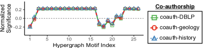
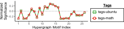
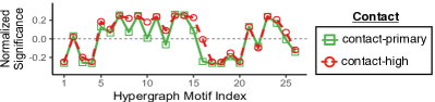
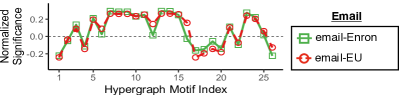
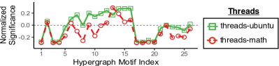
Figure 6: Characteristic profiles (CPs) capture local structural patterns of real-world hypergraphs accurately. The CPs are similar within domains but different across domains. Note that the significance of h-motif 3 distinguishes the contact hypergraphs from the email hypergraphs.

H-motifs in Tags Hypergraphs: In addition to instances of h-motif $11$, which are common in most real hypergraphs, instances of h-motif $16$, where all seven regions are not empty (see Figure 3), are particularly frequent in both tags datasets than in corresponding random hypergraphs.

H-motifs in Threads Hypergraphs: Lastly, in both data sets from the threads domain, instances of h-motifs $12$ and $24$ are noticeably more frequent than expected from the corresponding random hypergraphs.

In Appendix E, we analyze how the significance of each h-motif is correlated with the global structural properties of hypergraphs.

6.3 Q2. Comparison across Domains

We compare the characteristic profiles (CPs) of the real-world hypergraphs. In Figure 6, we present the CPs (i.e., the significances of the $26$ h-motifs) of each hypergraph. As seen in the figure, hypergraphs from the same domains have similar CPs. Specifically, all three hypergraphs from the co-authorship domain share extremely similar CPs, even when the absolute counts of h-motifs in them are several orders of magnitude different. Similarly, the CPs of both hypergraphs from the tags domain are extremely similar. However, the CPs of the three hypergraphs from the co-authorship domain are clearly distinguished by them of the hypergraphs from the tags domain. While the CPs of the hypergraphs from the contact domain and the CPs of those from the email domain are similar for the most part, they are distinguished by the significance of h-motif 3. These observations confirm that CPs accurately capture local structural patterns of real-world hypergraphs.

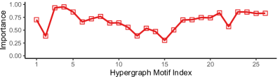
Figure 7: Importance of h-motifs in differentiating hypergraph domains: All 26 h-motifs contribute to distinguishing hypergraph domains, with each h-motif having varying levels of importance.

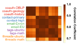
(a) Similarity matrix based on network motifs

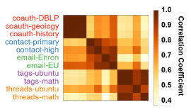
(b) Similarity matrix based on hypergraph motifs (h-motifs)

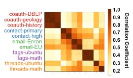
(c) Similarity matrix based on ternary hypergraph motifs (3h-motifs)

	Network Motifs	H-Motifs	3H-Motifs
(1) Average Similarity within Domains	0.988	0.978	0.932
(2) Average Similarity across Domains	0.919	0.654	0.370
Gap between (1) and (2)	0.069	0.324	0.562
Clustering Performance (NMI Score)	0.678	0.905	1.000

(d) Numerical comparisons of the similarity matrices

Figure 8: Real-world hypergraphs from the same domain exhibit similar characteristic profiles (CPs), while those from different domains have distinct CPs. Notably, the CPs based on h-motifs and 3h-motifs capture local structural patterns more accurately than those based on network motifs, as supported numerically in the table.

Importance of H-motifs: Since some h-motifs can be more useful than others, we measure the importance of each h-motif in distinguishing the domains of hypergraphs. We define the importance of a h-motif as its contribution to differentiating the domains of hypergraphs. The importance of each h-motif $t$ is defined as:

$$importance[t]=1-\frac{dist_{within}[t]}{dist_{across}[t]},$$

where $dist_{within}[t]$ is the average CP distance between hypergraphs from the same domain, and $dist_{across}[t]$ is the average CP distance between hypergraphs from different domains. As seen in Figure 7, all $26$ h-motifs have positive importances, indicating that all h-motifs do contribute to distinguishing the domains of hypergraphs. Note that each h-motif has different importance: some h-motifs are extremely important (e.g., h-motifs $3$, $4$, and $23$), while some are less important (e.g., h-motifs $2$, $12$, and $15$). It is important to note that these importance scores should be interpreted with caution, as they may be overfitted given the limited number of datasets (specifically, the similarities observed in 7 within-domain pairs and 48 cross-domain pairs).

6.4 Q3. Comparison of Characterization Powers

We compare the characterization power of h-motifs, 3h-motifs, and basic network motifs. Through this comparison, we demonstrate the effectiveness of h-motifs and 3h-motifs in capturing the structural properties of real-world hypergraphs.

CPs Based on Network Motifs: In addition to characteristic profiles (CPs) based on h-motifs and 3h-motifs, we additionally compute CPs based on network motifs. Specifically, we construct the incidence graph $G^{\prime}$ (defined in Section 2.1) of each hypergraph $G=(V,E)$. Then, we compute the CPs based on the network motifs consisting of $3$ to $5$ nodes, using bressan2019motivo . Using each of the three types of CPs, we compute the similarity matrices (specifically, correlation coefficient matrices) of the real-world hypergraphs and provide them in Figure 8.

Comparison of Pearson Correlations: As seen in Figures 8(a), 8(b) and 8(d), the domains of the real-world hypergraphs are distinguished more clearly by the CPs based on h-motifs than by the CPs based on network motifs. Numerically, when the CPs based on h-motifs are used, the average correlation coefficient is $0.978$ within domains and $0.654$ across domains, and the gap is $0.324$. However, when the CPs based on network motifs are used, the average correlation coefficient is $0.988$ within domains and $0.919$ across domains, and the gap is just $0.069$. As seen in Figures 8(c) and 8(d), the hypergraph domains are distinguished even more distinctly differentiated by the CPs based on 3h-motifs. Using 3h-motifs as a basis for the CPs results in significantly lower correlation coefficients between the contact and email domains, as well as between the tag and thread domains, allowing for a better distinction between these domains. Numerically, when 3h-motifs are used, the average correlation coefficient is $0.932$ within domains and $0.370$ across domains, and the gap is $0.562$. These results support that h-motifs and 3h-motifs play a key role in capturing local structural patterns of real-world hypergraphs.

Comparison of Clustering Performances: We further compare the characterization powers by evaluating clustering performance using each similarity matrix as the input for spectral clustering scikit-learn . We set the target number of clusters to the number of hypergraph domains. As summarized in Figure 8(d), the NMI scores, where higher scores indicate better clustering performance, are $0.678$, $0.905$, and $1$ when network motifs, h-motifs, and 3h-motifs, respectively, are used as a basis for the CPs. Notably, when 3h-motifs are used, the hypergraph domains are perfectly classified into distinct clusters. These results confirm again the effectiveness of h-motifs and 3h-motifs in characterizing real-world hypergraphs.

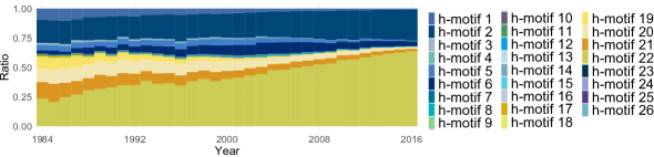
(a) Fraction of the instances of each h-motif in the coauth-DBLP dataset over time.

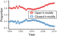
(b) Open and closed h-motifs.

Figure 9: Trends in the formation of collaborations are captured by h-motifs. (a) The fractions of the instances of h-motifs 2 and 22 have increased rapidly. (b) The fraction of the instances of open h-motifs has increased steadily since 2001.

6.5 Q4. Machine Learning Applications

We demonstrate that h-motifs and 3h-motifs provide useful input features for two machine learning tasks.

Hyperedge Prediction: We first consider the task of predicting future hyperedges in the seven real-world hypergraphs where MoCHy-E completes within a reasonable duration. As in yoon2020much , we formulate this problem as a binary classification problem, aiming to classify real hyperedges and fake ones. To this end, we create fake hyperedges in both training and test sets by replacing some fraction of nodes in each real hyperedge with random nodes. Refer to Appendix J for detailed settings. Then, we train classifiers using each of the following sets of input hyperedge features:

• HP26 ($\in\mathbb{R}^{26}$): HP based on h-motifs.

• HP7 ($\in\mathbb{R}^{7}$): The seven features with the largest variance among those in HP based on h-motifs.

• THP ($\in\mathbb{R}^{431}$): HP based on 3h-motifs.

• BASELINE ($\in\mathbb{R}^{7}$): The mean, maximum, and minimum degree and the mean, maximum, and minimum number of neighbors of the nodes in each hyperedge and its size.

We employ XGBoost chen2016xgboost as the classifier since it outperforms other classifiers, specifically logistic regression, random forest, decision tree, and multi-layer perception, on average, regardless of the feature sets used. Results with other classifiers can be found in Appendix J.

We report the accuracy (ACC) and the area under the ROC curve (AUC) in each setting in Table 4. Using HP26 and HP7, which are based on h-motifs, yields consistently better predictions than using BASELINE, which is a baseline feature set. In addition, using THP, which is based on 3h-motifs, leads to the best performance in almost all settings. These results suggest that h-motifs provide informative hyperedge features, and 3h-motifs provide even stronger hyperedge features for hyperedge prediction.

Table 4: H-motifs and 3h-motifs give informative hyperedge features. The use of h-motifs and 3h-motifs for input features in HP26 and THP, respectively, consistently outperforms using the baseline features in BASELINE for predicting hyperedges in all datasets. Even when reducing the dimension of HM26 to that of BASELINE (i.e., using HP7), the accuracy of predictions using h-motif-based features remains superior. For each setting, the best result is in bold and the second best one is underlined. The standard deviations of all the results are smaller than $0.0001$.

		HP26	HP7	THP	BASELINE
coauth-DBLP	ACC	0.801	0.744	0.836	0.646
	AUC	0.886	0.820	0.909	0.707
coauth-MAG-Geology	ACC	0.782	0.722	0.819	0.661
	AUC	0.865	0.798	0.892	0.741
coauth-MAG-History	ACC	0.696	0.683	0.716	0.608
	AUC	0.811	0.761	0.820	0.732
contact-primary-school	ACC	0.772	0.769	0.779	0.603
	AUC	0.879	0.868	0.886	0.647
contact-high-school	ACC	0.907	0.860	0.904	0.585
	AUC	0.968	0.949	0.967	0.641
email-Enron	ACC	0.815	0.725	0.827	0.633
	AUC	0.922	0.816	0.921	0.701
email-Eu	ACC	0.911	0.878	0.920	0.702
	AUC	0.972	0.954	0.977	0.781

Table 5: H-motifs and 3h-motifs provide valuable input features for node classification, with 3h-motifs showing particularly strong performance. The use of them for input features in NP26 and TNP yields better classification results than using the baseline features in BASELINE. For each metric, the best result is in bold and the second best one is underlined. The standard deviations of all the results are smaller than $0.0001$.

	NP26	NP7	TNP	BASELINE
ACC	0.682	0.545	0.723	0.659
AVG AUC	0.952	0.901	0.967	0.950

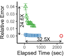
(a) threads-ubuntu

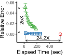
(b) email-Eu

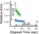
(c) contact-primary

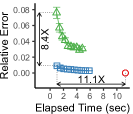
(d) coauth-history

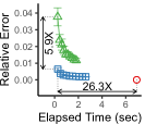
(e) contact-high

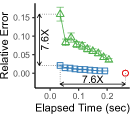
(f) email-Enron

Figure 10: MoCHy-A⁺ gives the best trade-off between speed and accuracy. It yields up to $25\times$ more accurate estimation than MoCHy-A, and it is up to $32.5\times$ faster than MoCHy-E. The error bars indicate $\pm$ $1$ standard error over $20$ trials.

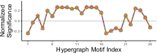
(a) email-EU

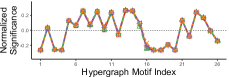
(b) contact-primary

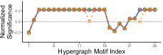
(c) coauth-history

Figure 11: Using MoCHy-A⁺, characteristic profiles (CPs) can be estimated accurately from a small number of samples.

Node Classification: As another machine learning application, we consider the task of node classification, where the label of each node is the hypergraph it belongs to. Since we utilize all eleven real-world hypergraphs, each node can have one of eleven possible labels. We draw 100 nodes uniformly at random from each hypergraph, and we use $80\%$ of them for training and the remaining $20\%$ of them for testing. Refer to Appendix K for detailed experimental settings. We train four classifiers using each of the following sets of input node features:

• NP26 ($\in\mathbb{R}^{26}$): NP based on h-motifs.

• NP7 ($\in\mathbb{R}^{7}$): The seven features with the largest variance among those in NP based on h-motifs.

• TNP ($\in\mathbb{R}^{431}$): NP based on 3h-motifs.

• BASELINE ($\in\mathbb{R}^{7}$): The node count, hyperedge count, average hyperedge size, average overlapping size, density hu2017maintaining , overlapness lee2021hyperedges , and the number of hyperedges that contain the ego-node in each ego-network.

For all feature sets, we use radial ego-networks as the ego-networks and XGBoost chen2016xgboost as the classifier. This is because using radial ego-networks and XGBoost gives better classification results than using other types of ego-networks and other classifiers in most cases. Refer to Appendix K for full experimental results with other types of ego-networks and other classifiers.

We report the accuracy (ACC) and the average area under the ROC curve (AVG AUC) in each setting in Table 5. Using TNP, which is based on 3h-motifs, yields the best classification result. Using NP26, which is based on h-motifs, outperforms using BASELINE, which is a baseline feature set. However, reducing the dimension of NP26 to that of BASELINE results in the worst performance. These results demonstrate that h-motifs and particularly 3h-motifs provide effective input features for node classification, highlighting the importance of local structural patterns in hypergraphs for this task.

6.6 Q5. Further Observations

We analyze the evolution of the co-authorship Hypergraphs by employing h-motifs. The dataset contains bibliographic information on computer science publications. Using the publications in each year from $1984$ to $2016$, we create $33$ hypergraphs where each node corresponds to an author, and each hyperedge indicates the set of the authors of a publication. Then, we compute the fraction of the instances of each h-motif in each hypergraph to analyze patterns and trends in the formation of collaborations. As shown in Figure 9, over the 33 years, the fractions have changed with distinct trends. First, as seen in Figure 9(b), the fraction of the instances of open h-motifs has increased steadily since 2001, indicating that collaborations have become less clustered, i.e., the probability that two collaborations intersecting with a collaboration also intersect with each other has decreased. Notably, the fractions of the instances of h-motif $2$ (closed) and h-motif $22$ (open) have increased rapidly, accounting for most of the instances.

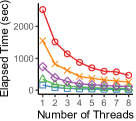
(a) Elapsed time on threads-ubuntu

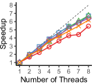
(b) Speedup on threads-ubuntu

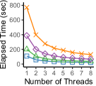
(c) Elapsed time on coauth-DBLP

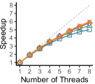
(d) Speedup on coauth-DBLP

Figure 12: Both MoCHy-E and MoCHy-A⁺ achieve significant speedups with multiple threads.

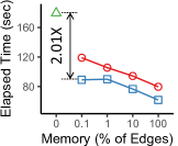
(a) Speedup $r$=1M

(b) Speedup $r$=1M

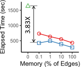
(c) Elapsed Time $r$=8M

(d) Speedup $r$=8M

Figure 13: On-the-fly MoCHy-A⁺ (Basic) and On-the-fly MoCHy-A⁺ (Adv.) achieve substantial speed improvements, compared to MoCHy-A⁺ without memoization, even when memoizing a small fraction of line graphs Between the two methods, On-the-fly MoCHy-A⁺ (Adv.) is faster up to $1.72\times$ than On-the-fly MoCHy-A⁺ (Basic), due to its carefully ordered processing scheme for sampled hyperwedges.

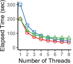
(a) Elapsed Time

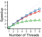
(b) Speedup

Figure 14: MoCHy-A⁺ for counting the instances of h-motifs is consistently faster than Motivo bressan2019motivo , which counts the instances of network motifs of size up to $5$, across different numbers of threads. When counting 3h-motifs, MoCHy-A⁺ is faster than Motivo with five or more threads. This is attributed to the fact that MoCHy-A⁺ exhibits better speedup as the number of threads increases compared to Motivo.

6.7 Q6. Performance of Counting Algorithms

We test the speed and accuracy of all versions of MoCHy under various settings. To this end, we measure elapsed time and relative error defined as

$$\frac{\sum_{t=1}^{26}|M[t]-\bar{M}[t]|}{\sum_{t=1}^{26}M[t]}\text{ and }\frac{\sum_{t=1}^{26}|M[t]-\hat{M}[t]|}{\sum_{t=1}^{26}M[t]},$$

for MoCHy-A and MoCHy-A⁺, respectively. Unless otherwise stated, we use a single thread without the on-the-fly computation scheme.

Speed and Accuracy: In Figure 10, we report the elapsed time and relative error of all versions of MoCHy on the $6$ different datasets where MoCHy-E terminates within a reasonable time. The numbers of samples in MoCHy-A and MoCHy-A⁺ are set to $\{2.5\times k:1\leq k\leq 10\}$ percent of the counts of hyperedges and hyperwedges, respectively. MoCHy-A⁺ provides the best trade-off between speed and accuracy. For example, in the threads-ubuntu dataset, MoCHy-A⁺ provides $24.6\times$ lower relative error than MoCHy-A, consistently with our theoretical analysis (see the last paragraph of Section 4.3). Moreover, in the same dataset, MoCHy-A⁺ is $32.5\times$ faster than MoCHy-E with little sacrifice on accuracy.

Effects of the Sample Size on CPs: In Figure 11, we report the CPs obtained by MoCHy-A⁺ with different numbers of hyperwedge samples on $3$ datasets. Even with a smaller number of samples, the CPs are estimated near perfectly.

Parallelization: We measure the running times of the proposed method with different numbers of threads on the threads-ubuntu and coauth-DBLP datasets. As seen in Figure 12, in both datasets, MoCHy achieves significant speedups with multiple threads. Specifically, with $8$ threads, MoCHy-E and MoCHy-A⁺ ($r=1M$) achieve speedups of $5.4$ and $6.7$, respectively in threads-ubuntu dataset. In the coauth-DBLP dataset, similar trends can be observed with speedups of $5.0$ and $6.0$ when using MoCHy-A⁺ for $r=1M$ and $r=8M$, respectively. MoCHy-E cannot be tested on the coauth-DBLP dataset since it does not complete within a reasonable duration.

Effects of On-the-fly Computation on Speed: We analyze the effects of the on-the-fly computation of line graphs (discussed in Section 4.4) on the speed of MoCHy-A⁺ under different memory budgets for memoization. To this end, we use the coauth-DBLP dataset, and we set the memory budgets so that up to {0%, 0.1%, 1%, 10%, 100%} of the edges in the line graph can be memoized. When the budget is $0\%$, we compute the neighbors of each hyperedge within the sampled hyperwedge every time, without precomputing or memoizing (a part of) the line graph. As shown in Figure 13, both On-the-fly MoCHy-A⁺ (Basic) and On-the-fly MoCHy-A⁺ (Adv.) faster than MoCHy-A⁺ without memoization, and their speed tends to improve as the memory budget increases. In addition, On-the-fly MoCHy-A⁺ (Adv.) is consistently faster than On-the-fly MoCHy-A⁺ (Basic) across different memory budgets. Specifically, it achieves up to $1.72\times$ reduced runtime, demonstrating the effectiveness of its carefully ordered processing schemes for sampled hyperwedges.

Comparison with Network-motif Counting: We assess the computational time needed for counting the instances of h-motifs, 3h-motifs, and network motifs on the coauth-DBLP dataset, which is our largest dataset. We employ MoCHy-A⁺ for both h-motifs and 3h-motifs, and for network motifs, we utilize Motivo bressan2019motivo , a recently introduced algorithm, to count the instances of network motifs up to size 5. In all cases, we fix the sample size to 2 million. As shown in Figure 14(a), when counting instances of h-motifs, MoCHy-A⁺ is consistently faster than Motivo across different numbers of threads, and the gap increases as the number of threads grows. When it comes to counting 3h-motifs, MoCHy-A⁺ is slower than Motivo with a single thread, but it becomes faster with five or more threads. This is attributed to MoCHy-A⁺ achieving significant speedups with more threads, compared to Motivo, as shown in Figure 14(b).

7 Related Work

We review prior work on network motifs, algorithms for counting them, and hypergraphs. While the definition of a network motif varies among studies, here we define it as a connected graph composed by a predefined number of nodes.

Network Motifs. Network motifs were proposed as a tool for understanding the underlying design principles and capturing the local structural patterns of graphs holland1977method ; shen2002network ; milo2002network . The occurrences of motifs in real-world graphs are significantly different from those in random graphs milo2002network , and they vary also depending on the domains of graphs milo2004superfamilies . The concept of network motifs has been extended to various types of graphs, including dynamic paranjape2017motifs graphs, bipartite graphs borgatti1997network , heterogeneous graphs rossi2019heterogeneous , and simplicial complexes benson2018simplicial ; kim2023characterization ; preti2022fresco The occurrences of network motifs have been used in a wide range of graph applications: community detection benson2016higher ; tsourakakis2017scalable ; yin2017local ; li2019edmot , ranking zhao2018ranking , graph embedding rossi2018higher ; yu2019rum , and graph neural networks lee2019graph , to name a few.

Algorithms for Network Motif Counting. We focus on algorithms for counting the occurrences of every network motif whose size is fixed or within a certain range ahmed2015efficient ; ahmed2017graphlet ; aslay2018mining ; bressan2019motivo ; chen2016general ; han2016waddling ; pinar2017escape , while many are for a specific motif (e.g., the clique of size $3$) ahmed2017sampling ; de2016triest ; hu2013massive ; hu2014efficient ; jha2013space ; kim2014opt ; ko2018turbograph ; pagh2012colorful ; sanei2018butterfly ; shin2017wrs ; shin2020fast ; tsourakakis2009doulion ; wang2019rept ; wang2017approximately . Given a graph, they aim to count rapidly and accurately the instances of motifs with $4$ or more nodes, despite the combinatorial explosion of the instances, using the following techniques:

1. Combinatorics: For exact counting, combinatorial relations between counts have been employed ahmed2015efficient ; pinar2017escape ; paranjape2017motifs . That is, prior studies deduce the counts of the instances of motifs from those of other smaller or equal-size motifs.

2. MCMC: Most approximate algorithms sample motif instances from which they estimate the counts. Based on MCMC sampling, the idea of performing a random walk over instances (i.e, connected subgraphs) until it reaches the stationarity to sample an instance from a fixed probability distribution (e.g., uniform) has been employed bhuiyan2012guise ; chen2016general ; han2016waddling ; saha2015finding ; wang2014efficiently ; matsuno2020improved .

3. Color Coding: Instead of MCMC, color coding alon1995color can be employed for sampling bressan2017counting ; bressan2019motivo ; bressan2021faster . Specifically, prior studies color each node uniformly at random among $k$ colors, count the number of $k$-trees with $k$ colors rooted at each node, and use them to sample instances from a fixed probability distribution.

In our problem, which focuses on h-motifs with only $3$ hyperedges, sampling instances with fixed probabilities is straightforward without (2) or (3), and the combinatorial relations on graphs in (1) are not applicable. In algorithmic aspects, we address the computational challenges discussed at the beginning of Section 4 by answering (a) what to precompute (Section 4.1), (b) how to leverage it (Sections 4.2 and 4.3), and (c) how to prioritize it (Sections 4.4 and 6.7), with formal analyses (Lemma 2; Theorems 4.1, 4.3, and 4.6).

Hypergraph Mining. Hypergraphs naturally represent group interactions occurring in a wide range of fields, including computer vision huang2010image ; yu2012adaptive , bioinformatics hwang2008learning , circuit design karypis1999multilevel ; ouyang2002multilevel , social network analysis li2013link ; yang2019revisiting , cryptocurrency kim2022reciprocity , and recommender systems bu2010music ; li2013news . There also has been considerable attention on machine learning on hypergraphs, including clustering agarwal2005beyond ; amburg2019hypergraph ; karypis2000multilevel ; lee2022tri ; zhou2007learning , classification jiang2019dynamic ; lee2022tri ; sun2008hypergraph ; yu2012adaptive , hyperedge prediction benson2018simplicial ; yoon2020much ; zhang2018beyond ; hwang2022ahp , and anomaly detection lee2022hashnwalk . Recent studies on real-world hypergraphs revealed interesting patterns commonly observed across domains, including (a) global structural properties (e.g., giant connected components and small diameter) do2020multi ; ko2022growth ; bu2023hypercore and their temporal evolution (e.g., shrinking diameter) ko2022growth ; (b) structural properties of ego-networks (e.g., density and overlapness) lee2021hyperedges and their temporal evolution (e.g., decreasing rates of novel nodes) comrie2021hypergraph ; and (c) temporal patterns regarding arrivals of the same or overlapping hyperedges benson2018sequences ; choo2022persistence ; cencetti2021temporal . Notably, Benson et al. benson2018simplicial studied how several local features, including edge density, average degree, and probabilities of simplicial closure events for $4$ or less nodes, differ across domains. Our analysis using h-motifs is complementary to these approaches in that it (1) captures local patterns systematically without hand-crafted features, (2) captures static patterns without relying on temporal information, and (3) naturally uses hyperedges with any number of nodes without decomposing them into small ones.

Recently, there has been an extension of hypergraph motifs to temporal hypergraphs, which evolve over time lee2021thyme+ ; lee2023temporal . This extension introduces 96 temporal hypergraph motifs (TH-motifs) that capture not only the overlapping patterns but also the relative order among three connected hyperedges. This extension has been shown to improve the characterization power of h-motifs in hypergraph classification and hyperedge prediction tasks. Along with the concept of TH-motifs, a family of algorithms has been proposed for the exact and approximate counting of TH-motifs. The focuses of the algorithms are the dynamic update of the line graph over time and the prioritized sampling of time intervals for estimation. It is important to note that this conceptual and algorithmic extension requires temporal information as input, and is orthogonal to our extension to 3h-motifs, which only requires topological information.

8 Conclusions and Future Directions

In this section, we present conclusions and future research directions.

8.1 Conclusions

In this work, we introduce hypergraph motifs (h-motifs), and their extensions, ternary hypergraph motifs (3h-motifs). Using them, we investigate the local structures of $11$ real-world hypergraphs from $5$ different domains. We summarize our contributions as follows:

• Novel Concepts: We define 26 h-motifs, which describe connectivity patterns of three connected hyperedges in a unique and exhaustive way, independently of the sizes of hyperedges (Figure 3). We extend this concept to 431 3h-motifs, enabling a more specific differentiation of local structures (Figure 5).

• Fast and Provable Algorithms: We propose $3$ parallel algorithms for (approximately) counting every h-motif’s instances, and we theoretically and empirically analyze their speed and accuracy. Both approximate algorithms yield unbiased estimates (Theorems 4.2 and 4.5), and especially the advanced one is up to $32\times$ faster than the exact algorithm, with little sacrifice on accuracy (Figure 10).

• Discoveries in $11$ Real-world Hypergraphs: We confirm the efficacy of h-motifs and 3h-motifs by showing that local structural patterns captured by them are similar within domains but different across domains (Figures 6 and 8).

• Machine Learning Applications: Our experiments have shown that h-motifs are effective in extracting features for hypergraphs, hyperedges, and nodes in tasks such as hypergraph clustering, hyperedge prediction, and node classification. Furthermore, using 3h-motifs has been demonstrated to improve the feature extraction capabilities, resulting in even better performances on these applications.

8.2 Future Research Directions

Future directions include exploring the practical applications of h-motifs and 3h-motifs, motivated by the numerous successful use cases of network motifs in practical applications. For example, network motifs have been used in the domain of biology, for identifying crucial interactions between proteins, DNA, and metabolites within biological networks yeger2004network ; ma2004extended . Another compelling example lies within mobile communication networks, where network motifs have been observed to significantly impact the efficiency of information delivery across users zhang2022influence . In addition, network motifs are proven to be powerful tools for enhancing the performance of other practical applications including anomaly detection noble2003graph ; yuan2021higher and recommendation gupta2014real ; zhao2019motif ; sun2022motifs ; cui2021motif . Furthermore, they are recognized as a useful ingredient when designing graph-related algorithms, such as graph neural networks sankar2017motif ; yu2022molecular and graph clustering algorithms yin2017local ; benson2016higher . These examples demonstrate the substantial potential of h-motifs in diverse applications, and notably, most of them are less explored in hypergraphs than in graphs.

In Sections 6.4 and 6.5, we demonstrated the critical role of h-motifs and 3h-motifs in enhancing performance across hypergraph learning tasks, including node classification and hyperedge prediction We believe that the considered hypergraph learning tasks can be readily applied to practical applications choe2023classification ; antelmi2023survey . For example, to achieve effective educational management and evaluation, it is important to classify the academic performance (e.g., poor, medium, and excellent) of students (nodes) based on the associations (hyperedges) among them li2022multi . It is also crucial to classify fake news (nodes) based on the patterns of news consumption by users (hyperedges) jeong2022nothing . Accurately identifying labels for objects (nodes) in images (hyperedges) containing multiple entities is a crucial task in computer vision wu2020adahgnn . Refer to a survey antelmi2023survey for a broader range of applications formulated as node classification on hypergraphs. In addition, hyperedge prediction can be employed for identifying novel sets (e.g., outfits) of items (e.g., fashion items) to be purchased together li2021hyperbolic (b) suggesting novel combinations of ingredients for recipes  zhang2018beyond , (c) recommending new collaborations among researchers liu2018context , and (d) discovering groups of genes collaborating for specific biological functions nguyen2022sparse . As we demonstrated in Sections 6.4 and 6.5, h-motifs and 3h-motifs serve as valuable tools for addressing such tasks, indicating their potential applicability in practical scenarios, which we leave for future work.

Other promising research directions include (a) extending h-motifs and 3h-motifs to complex and rich hypergraphs, such as labeled or heterogeneous hypergraphs, and (b) investigating alternative random hypergraph models for assessing the significance of h-motifs and 3h-motifs.

Reproducibility: The code and datasets used in this work are available at https://github.com/jing9044/MoCHy-with-3h-motif.

Appendix A Proof of Theorem 2

We let $X_{ij}[t]$ be a random variable indicating whether the $i$-th sampled hyperedge (in line 4 of Algorithm 4) is included in the $j$-th instance of h-motif $t$ or not. That is, $X_{ij}[t]=1$ if the hyperedge is included in the instance, and $X_{ij}[t]=0$ otherwise. We let $\bar{m}[t]$ be the number of times that h-motif $t$’s instances are counted while processing $s$ sampled hyperedges. That is,

$$\bar{m}[t]:=\sum_{i=1}^{s}\sum_{j=1}^{M[t]}X_{ij}[t].$$ (9)

Then, by lines 4-4 of Algorithm 4,

$$\bar{M}[t]=\bar{m}[t]\cdot\tfrac{|E|}{3s}.$$ (10)

Proof of the Bias of $\bar{M}[t]$ (Eq. (4)): Since each h-motif instance contains three hyperedges, the probability that each $i$-th sampled hyperedge is contained in each $j$-th instance of h-motif $t$ is

$$P[X_{ij}[t]=1]=\mathbb{E}[X_{ij}[t]]=\tfrac{3}{|E|}.$$ (11)

From linearity of expectation,

$$\mathbb{E}[\bar{m}[t]]=\sum_{i=1}^{s}\sum_{j=1}^{M[t]}\mathbb{E}[X_{ij}[t]]=\sum_{i=1}^{s}\sum_{j=1}^{M[t]}\frac{3}{|E|}=\frac{3s\cdot M[t]}{|E|}.$$

Then, by Eq. (10), $\mathbb{E}[\bar{M}[t]]=\tfrac{|E|}{3s}\cdot\mathbb{E}[\bar{m}[t]]=M[t]$. ∎

Proof of the Variance of $\bar{M}[t]$ (Eq. (5)): From Eq. (11) and $X_{ij}[t]=X_{ij}[t]^{2}$, the variance of $X_{ij}[t]$ is

$$\mathbb{V}\mathrm{ar}[X_{ij}[t]]=\mathbb{E}[X_{ij}[t]^{2}]-\mathbb{E}[X_{ij}[t]]^{2}=\frac{3}{|E|}-\frac{9}{|E|^{2}}.$$ (12)

Consider the covariance between $X_{ij}[t]$ and $X_{i^{\prime}j^{\prime}}[t]$. If $i=i^{\prime}$, then from Eq. (11),

$$\mathbb{C}\mathrm{ov}(X_{ij}[t],X_{i^{\prime}j^{\prime}}[t])=\mathbb{E}[X_{ij}[t]\cdot X_{ij^{\prime}}[t]]-\mathbb{E}[X_{ij}[t]]\mathbb{E}[X_{ij^{\prime}}[t]]$$

$$=P[X_{ij}[t]=1,X_{ij^{\prime}}[t]=1]-\mathbb{E}[X_{ij}[t]]\mathbb{E}[X_{ij^{\prime}}[t]]$$

$$=P[X_{ij}[t]=1]\cdot P[X_{ij^{\prime}}[t]=1|X_{ij}[t]=1]$$

$$\hskip 10.0pt-\mathbb{E}[X_{ij}[t]]\mathbb{E}[X_{ij^{\prime}}[t]]$$

$$=\frac{3}{|E|}\cdot\frac{l_{jj^{\prime}}}{3}-\frac{9}{|E|^{2}}=\frac{l_{jj^{\prime}}}{|E|}-\frac{9}{|E|^{2}},\vspace{-1mm}$$ (13)

where $l_{jj^{\prime}}$ is the number of hyperedges that the $j$-th and $j^{\prime}$-th instances share. However, since hyperedges are sampled independently (specifically, uniformly at random with replacement), if $i\neq i^{\prime}$, then $\mathbb{C}\mathrm{ov}(X_{ij}[t],X_{i^{\prime}j^{\prime}}[t])=0$. This observation, Eq. (9), Eq. (12), and Eq. (13) imply

$$\mathbb{V}\mathrm{ar}[\bar{m}[t]]=\mathbb{V}\mathrm{ar}[\sum_{i=1}^{s}\sum_{j=1}^{M[t]}X_{ij}[t]]$$

$$=\sum_{i=1}^{s}\sum_{j=1}^{M[t]}\mathbb{V}\mathrm{ar}[X_{ij}[t]]+\sum_{i=1}^{s}\sum_{j\neq j^{\prime}}\mathbb{C}\mathrm{ov}(X_{ij}[t],X_{ij^{\prime}}[t])$$

$$=s\cdot M[t]\cdot(\frac{3}{|E|}-\frac{9}{|E|^{2}})+s\sum_{l=0}^{2}p_{l}[t](\frac{l}{|E|}-\frac{9}{|E|^{2}}),$$

where $p_{l}[t]$ is the number of pairs of h-motif $t$’s instances sharing $l$ hyperedges. This and Eq. (10) imply Eq. (5). ∎

Appendix B Proof of Theorem 4

Let $\tau:=M[t]\cdot\epsilon$ and $X_{ij}[t]$ be a random variable indicating whether the $i$-th sampled hyperedge (in line 4 of Algorithm 4) is included in the $j$-th instance of h-motif $t$ or not. Also, let $\tilde{X}_{i}[t]=\frac{|E|}{3s}\sum_{j=1}^{M[t]}X_{ij}[t]$ (where the sum indicates the number of instances of h-motif t that contains i-th sampled hyperedge) so that $\bar{M}[t]=\sum_{i=1}^{s}\tilde{X}_{i}[t]$. Note that $0\leq\tilde{X}_{i}[t]\leq\frac{|E|d_{\max}[t]^{2}}{3s}$ holds for every $i$. Since $\tilde{X}_{1}[t],\tilde{X}_{2}[t],\dots,\tilde{X}_{s}[t]$ are independent random variables and $\mathbb{E}[\bar{M}[t]]=M[t]$ (Theorem 4.2), we can apply Hoeffding’s inequality (Lemma 3):

$$\Pr [|\bar{M}[t]-M[t]|\geq M[t]\cdot\epsilon]$$

$$\leq 2\exp\left(-\frac{2\epsilon^{2}M[t]^{2}}{s\cdot(d_{\max}[t]^{2}|E|/3s)^{2}}\right)$$

$$\leq 2\exp(-\frac{18s\epsilon^{2}M[t]^{2}}{|E|^{2}d_{\max}[t]^{4}})\leq\delta,$$

which implies the condition for the sample size. ∎.

Appendix C Proof of Theorem 5

A random variable $Y_{ij}[t]$ denotes whether the $i$-th sampled hyperwedge (in line 5 of Algorithm 5) is included in the $j$-th instance of h-motif $t$. That is, $Y_{ij}[t]=1$ if the sampled hyperwedge is included in the instance, and $Y_{ij}[t]=0$ otherwise. We let $\hat{m}[t]$ be the number of times that h-motif $t$’ instances are counted while processing $r$ sampled hyperwedges. That is,

$$\hat{m}[t]:=\sum_{i=1}^{r}\sum_{j=1}^{M[t]}Y_{ij}[t]$$ (14)

We use $w[t]$ to denote the number of hyperwedges included in each instance of h-motif $t$. That is,

$$w[t]:=\begin{cases}2&\text{if h-motif $t$ is open,}\\ 3&\text{if h-motif $t$ is closed.}\end{cases}$$ (15)

Then, by lines 5-5 of Algorithm 5,

$$\hat{M}[t]=\hat{m}[t]\cdot\tfrac{1}{w[t]}\cdot\tfrac{|\wedge|}{r}.$$ (16)

Proof of the Bias of $\hat{M}[t]$ (Eq. (6)): Since each instance of h-motif $t$ contains $w[t]$ hyperwedges, the probability that each $i$-th sampled hyperwedge is contained in each $j$-th instance of h-motif $t$ is

$$P[Y_{ij}[t]=1]=\mathbb{E}[Y_{ij}[t]]=\tfrac{w[t]}{|\wedge|}.$$ (17)

From linearity of expectation,

$$\mathbb{E}[\hat{m}[t]]=\sum_{i=1}^{r}\sum_{j=1}^{M[t]}\mathbb{E}[Y_{ij}[t]]=\sum_{i=1}^{r}\sum_{j=1}^{M[t]}\frac{w[t]}{|\wedge|}=\frac{w[t]\cdot r\cdot M[t]}{|\wedge|}.$$

Then, by Eq. (16), $\mathbb{E}[\hat{M}[t]]=\mathbb{E}[\hat{m}[t]]\cdot\tfrac{1}{w[t]}\cdot\tfrac{|\wedge|}{r}=M[t]$. ∎

Proof of the Variance of $\hat{M}[t]$ (Eq. (7) and Eq. (8):
From Eq. (17) and $Y_{ij}[t]=Y_{ij}[t]^{2}$, the variance of each random variable $Y_{ij}[t]$ is

$$\mathbb{V}\mathrm{ar}[Y_{ij}[t]]=\mathbb{E}[Y_{ij}[t]^{2}]-\mathbb{E}[Y_{ij}[t]]^{2}=\frac{w[t]}{|\wedge|}-\frac{w[t]^{2}}{|\wedge|^{2}}.$$ (18)

Consider the covariance between $Y_{ij}[t]$ and $Y_{i^{\prime}j^{\prime}}[t]$. If $i=i^{\prime}$, then from Eq. (17),

$$\mathbb{C}\mathrm{ov}(Y_{ij}[t],Y_{i^{\prime}j^{\prime}}[t])=\mathbb{E}[Y_{ij}[t]\cdot Y_{ij^{\prime}}[t]]-\mathbb{E}[Y_{ij}[t]]\mathbb{E}[Y_{ij^{\prime}}[t]]$$

$$=P[Y_{ij}[t]=1,Y_{ij^{\prime}}[t]=1]-\mathbb{E}[Y_{ij}[t]]\mathbb{E}[Y_{ij^{\prime}}[t]]$$

$$=P[Y_{ij}[t]=1]\cdot P[Y_{ij^{\prime}}[t]=1|Y_{ij}[t]=1]-\mathbb{E}[Y_{ij}[t]]\mathbb{E}[Y_{ij^{\prime}}[t]]$$

$$=\frac{w[t]}{|\wedge|}\cdot\frac{n_{jj^{\prime}}}{w[t]}-\frac{w[t]^{2}}{|\wedge|^{2}}=\frac{n_{jj^{\prime}}}{|\wedge|}-\frac{w[t]^{2}}{|\wedge|^{2}},$$ (19)

where $n_{jj^{\prime}}$ is the number of hyperwedges that the $j$-th and $j^{\prime}$-th instances share. However, since hyperwedges are sampled independently (specifically, uniformly at random with replacement), if $i\neq i^{\prime}$, then $\mathbb{C}\mathrm{ov}(Y_{ij}[t],Y_{i^{\prime}j^{\prime}}[t])=0$. This observation, Eq. (14), Eq. (18), and Eq. (19) imply

$$\mathbb{V}\mathrm{ar}[\hat{m}[t]]=\mathbb{V}\mathrm{ar}[\sum_{i=1}^{r}\sum_{j=1}^{M[t]}Y_{ij}[t]]$$

$$=\sum_{i=1}^{r}\sum_{j=1}^{M[t]}\mathbb{V}\mathrm{ar}[Y_{ij}[t]]+\sum_{i=1}^{r}\sum_{j\neq j^{\prime}}\mathbb{C}\mathrm{ov}(Y_{ij}[t],Y_{ij^{\prime}}[t])$$

$$=r\cdot M[t]\cdot(\frac{w[t]}{|\wedge|}-\frac{w[t]^{2}}{|\wedge|^{2}})+r\sum_{n=0}^{1}q_{n}[t]\cdot(\frac{n}{|\wedge|}-\frac{w[t]^{2}}{|\wedge|^{2}}),$$

where $q_{n}[t]$ is the number of pairs of h-motif $t$’s instances that share $n$ hyperwedges. This and Eq. (16) imply Eq. (7) and Eq. (8). ∎

Appendix D Proof of Theorem 7

Let $\tau:=M[t]\cdot\epsilon$ and $Y_{ij}[t]$ denotes whether the $i$-th sampled hyperwedge (in line 5 of Algorithm 5) is included in the $j$-th instance of h-motif $t$. Also, let $\tilde{Y}_{i}[t]=\frac{|\Lambda|}{w[t]s}\sum_{j=1}^{M[t]}Y_{ij}[t]$ with $w[t]$ defined in Eq. (15), where the sum indicates the number of instances of h-motif $t$ that contains the $i$-th sampled hyperwedge, so that $\hat{M}[t]=\sum_{i=1}^{r}\tilde{Y}_{i}[t]$. Then, $0\leq\tilde{Y}_{i}[t]\leq\frac{|\Lambda|d_{\max}[t]}{w[t]r}$ holds for every $i$. Since $\tilde{Y}_{1}[t],\tilde{Y}_{2}[t],\dots,\tilde{Y}_{r}[t]$ are independent random variables and $\mathbb{E}[\hat{M}[t]]=M[t]$ (in Theorem 4.5), we can apply Hoeffding’s inequality:

$$\Pr \left[|\hat{M}[t]-M[t]|\geq M[t]\cdot\epsilon\right]$$

$$\leq 2\exp\left(-\frac{2\epsilon^{2}M[t]^{2}}{r\cdot(d_{\max}[t]|\Lambda|/w[t]r)^{2}}\right)$$

$$\leq 2\exp(-\frac{2\cdot w[t]^{2}r\epsilon^{2}M[t]^{2}}{|\Lambda|^{2}d_{\max}[t]^{2}})\leq\delta,$$

which implies the condition for the sample size. ∎.

Table 6: Global structural properties of real-world hypergraphs.

	Size		Average Degree		Clustering Coeff.		Effective Diamter	# of H-motifs
Dataset	Node	Hyperedge	Node	Hyperedge	Node	Hyperedge
coauth-DBLP	1,924,991	2,466,792	4.013	3.132	0.296	0.225	6.590	26.3B
coauth-geology	1,256,385	1,203,895	3.015	3.146	0.382	0.208	6.809	6B
coauth-history	1,014,734	895,439	1.354	1.535	0.575	0.331	12.946	83.2M
contact-primary	242	12,704	126.9	2.418	0.011	0.270	1.888	617M
contact-high	327	7,818	55.6	2.326	0.018	0.286	2.564	69.7M
email-Enron	143	1,512	31.8	3.009	0.064	0.249	2.583	9.6M
email-EU	998	25,027	85.9	3.425	0.030	0.207	2.836	7B
tags-ubuntu	3,029	147,222	164.8	3.391	0.007	0.182	2.262	4.3T
tags-math	1,629	170,476	364.1	3.479	0.005	0.180	2.189	9.2T
threads-ubuntu	125,602	166,999	2.538	1.908	0.160	0.301	4.657	11.4B
threads-math	176,445	595,749	8.261	2.446	0.033	0.250	3.662	2.2T

Appendix E Correlation between Global Structural Properties and H-motifs

We investigate the correlation between global structural properties and the hypergraph motifs (h-motifs). We consider eight global properties, categorized into five as follows.

• Size: We consider (1) the number of nodes and (2) the number of hyperedges.

• Average degree: The degree of a node is defined as the number of hyperedges that contain the node. The degree of a hyperedge is defined as the number of nodes that the hyperedge contains. We consider (3) the average degree of all nodes and (4) the average degree of all hyperedges.

• Clustering coefficients: In [35, 58], the clustering coefficient of two nodes $u\neq v$ is defined as:

  $$CC(u,v)=\frac{|E_{u}\cap E_{v}|}{|E_{u}\cup E_{v}|},$$

  where $E_{u}$ is the set of hyperedges that contain the node $u$. Then, the average clustering coefficient of each node is defined as the mean of the clustering coefficients of it and each of its neighbors, i.e.,

  $$CC(u)=\frac{\sum_{v\in N_{u}}CC(u,v)}{|N_{u}|},$$

  where $N_{u}$ is the set of neighbors of node $u$ (i.e., $\{v\in V:E_{u}\cap E_{v}\neq\emptyset\}$). Similarly, we can define the clustering coefficients of hyperedge pairs and those of hyperedges. We consider (5) the mean of the clustering coefficients of all nodes and (6) the mean of the clustering coefficients of all hyperedges.

• Effective diameter: The diameter of a graph is defined as the maximum length of the shortest paths in the graph. Similarly, we define (7) the diameter of a hypergraph as the maximum length of the shortest hyperpaths in the hypergraph. In hypergraphs, a hyperpath between two nodes $v_{1}$ and $v_{k}$ is a sequence of distinct nodes and hyperedges $v_{1}$, $e_{1}$, $v_{2}$, $e_{2}$, …,$e_{k-1}$, $v_{k}$ where there $v_{i}\in e_{i}$ and $v_{i+1}\in e_{i}$ for $1\leq i<k$ [121]. The length of a hyperpath is the number of intermediate hyperedges contained in the hyperpath. In hypergraphs that have disconnected components, the diameter is not computable. Thus, we compute effective diameter [84], which is the 90th percentile of the distribution of shortest-path lengths. We use GetAnfEffDiam function provided by [67].

• Total number of h-motifs: We consider (8) the total number of hypergraph motifs computed using MoCHy.

The statistics of the global properties of hypergraphs are provided in Table 6. We compute the Pearson correlation coefficients between each h-motif’s CP value and eight different global properties. As seen in Table 7, different h-motifs show different correlations with each global property. For example, h-motif 13 shows the lowest correlation with the node size ($-0.558$), the node-based clustering coefficient ($-0.650$), the hyperedge-based clustering coefficient ($-0.499$), and the effective diameter ($-0.620$), but the highest correlation with the average node degree ($0.523$) and the average hyperedge degree ($0.522$). In addition, some global properties are strongly correlated with h-motifs, while some are weakly correlated. For example, there are many h-motifs highly correlated with the node size, the node-based clustering coefficient, and the effective diameter, while most of the h-motifs have near-zero correlations with the average hyperedge degree and the hyperedge-based clustering coefficient.

Table 7: Correlation between global structural properties and characteristic profiles (CPs). Strong positive or negative correlations ($\geq 0.5$) are colored as red (positive) or blue (negative).

	Size		Average Degree		Clustering Coeff.		Effective Diamter	# of H-motifs
h-motif	Node	Hyperedge	Node	Hyperedge	Node	Hyperedge
1	$+0.787$	$+0.648$	$-0.497$	$+0.003$	$+0.751$	$+0.115$	$+0.626$	$-0.530$
2	$-0.169$	$-0.110$	$-0.023$	$-0.645$	$-0.027$	$+0.479$	$+0.099$	$+0.101$
3	$+0.710$	$+0.587$	$-0.492$	$+0.065$	$+0.718$	$+0.067$	$+0.633$	$-0.501$
4	$+0.901$	$+0.783$	$-0.480$	$-0.071$	$+0.891$	$+0.122$	$+0.806$	$-0.410$
5	$+0.469$	$+0.315$	$-0.506$	$-0.126$	$+0.498$	$+0.316$	$+0.406$	$-0.730$
6	$+0.877$	$+0.762$	$-0.311$	$-0.161$	$+0.872$	$+0.151$	$+0.801$	$-0.249$
7	$+0.229$	$+0.071$	$-0.436$	$-0.188$	$+0.313$	$+0.394$	$+0.215$	$-0.744$
8	$+0.388$	$+0.237$	$-0.561$	$-0.154$	$+0.447$	$+0.359$	$+0.361$	$-0.772$
9	$+0.138$	$-0.023$	$-0.266$	$-0.081$	$+0.229$	$+0.293$	$+0.124$	$-0.606$
10	$+0.444$	$+0.288$	$-0.584$	$-0.178$	$+0.537$	$+0.363$	$+0.447$	$-0.733$
11	$+0.123$	$-0.041$	$+0.023$	$+0.098$	$+0.200$	$+0.077$	$+0.087$	$-0.329$
12	$+0.611$	$+0.540$	$-0.246$	$-0.096$	$+0.676$	$+0.050$	$+0.643$	$-0.061$
13	$-0.558$	$-0.485$	$+0.523$	$+0.552$	$-0.650$	$-0.499$	$-0.620$	$+0.413$
14	$-0.490$	$-0.567$	$+0.232$	$+0.156$	$-0.351$	$-0.010$	$-0.417$	$-0.064$
15	$+0.166$	$+0.042$	$-0.148$	$+0.080$	$+0.299$	$+0.045$	$+0.224$	$-0.224$
16	$+0.481$	$+0.464$	$-0.184$	$+0.028$	$+0.531$	$-0.110$	$+0.532$	$+0.106$
17	$+0.754$	$+0.608$	$-0.501$	$-0.127$	$+0.828$	$+0.231$	$+0.741$	$-0.481$
18	$+0.442$	$+0.298$	$-0.444$	$+0.031$	$+0.551$	$+0.149$	$+0.473$	$-0.532$
19	$+0.623$	$+0.471$	$-0.507$	$-0.089$	$+0.677$	$+0.251$	$+0.584$	$-0.596$
20	$+0.628$	$+0.473$	$-0.483$	$-0.001$	$+0.724$	$+0.136$	$+0.633$	$-0.514$
21	$+0.089$	$-0.047$	$-0.315$	$-0.136$	$+0.141$	$+0.346$	$+0.074$	$-0.676$
22	$+0.554$	$+0.522$	$-0.157$	$-0.299$	$+0.724$	$+0.127$	$+0.763$	$+0.154$
23	$+0.332$	$+0.181$	$-0.434$	$-0.130$	$+0.365$	$+0.334$	$+0.273$	$-0.722$
24	$+0.428$	$+0.275$	$-0.492$	$-0.147$	$+0.459$	$+0.341$	$+0.368$	$-0.737$
25	$+0.747$	$+0.593$	$-0.508$	$-0.151$	$+0.758$	$+0.269$	$+0.666$	$-0.610$
26	$+0.883$	$+0.812$	$-0.330$	$-0.203$	$+0.877$	$+0.118$	$+0.830$	$-0.129$

Input : bipartite graph $G^{\prime}$: $G^{\prime}=(V\cup E,E^{\prime})$

Output : randomized bipartite graph $\tilde{G}=(V\cup E,\tilde{E})$

${\{d_{i}^{V}\}}_{i=1}^{|V|}\leftarrow$ degrees of nodes in $V$

1 ${\{d_{j}^{E}\}}_{j=1}^{|E|}\leftarrow$ degrees of nodes in $E$

2 $\tilde{E}\leftarrow$ an empty multiset      

3 for $k=1,...,|E^{\prime}|$  do

4       $v_{i}\leftarrow$ sample from $V$ with probability $\propto$ degree

5       $e_{j}\leftarrow$ sample from $E$ with probability $\propto$ degree

6       add $(v_{i},e_{j})$ to $\tilde{E}$

7      

return $\tilde{G}=(\tilde{V},\tilde{E})$

Algorithm 6 Chung-Lu Model [7]

Input : incidence graph $\tilde{G}=(V\cup E,\tilde{E})$

Output : hypergraph $\hat{G}=(V,\hat{E})$

1for each $\tilde{e}_{j}\in\tilde{E}$ do

2       $\hat{e}_{j}\leftarrow\varnothing$

3for each $(v_{i},e_{j})\in\tilde{E}$ do

4       $\hat{e}_{j}\leftarrow\hat{e}_{j}\cup\{v_{i}\}$

5      

6$\hat{E}\leftarrow\varnothing$

7 for each $e_{j}\in E$ do

8       if $\hat{e}_{j}\neq\varnothing$ then

9             $\hat{E}\leftarrow\hat{E}\cup\{\hat{e}_{j}\}$

return $\hat{G}=(V,\hat{E})$

Algorithm 7 Transformation from Incidence Graphs to Hypergraphs

Appendix F Randomized Hypergraphs

To create randomized hypergraphs, we extend the Chung-Lu model [7], which is a configuration model designed to generate random bipartite graphs, to hypergraphs. Algorithm 6 provides the pseudocode for the Chung-Lu model, where $V$ and $E$ represent two sets of nodes in both the input and output bipartite graphs. Note that the output bipartite graph $\tilde{G}$ allows parallel edges (i.e. $\tilde{E}$ is a multiset). The Chung-Lu model preserves the degrees of nodes in expectation, i.e., the following equalities hold:

$$\mathbb{E}[\tilde{d}_{i}^{V}]=d_{i}^{V},\ \mathbb{E}[\tilde{d}_{j}^{E}]=d_{j}^{E},$$ (20)

where $d_{i}^{V}$ and $d_{j}^{E}$ denote the degrees of nodes $v_{i}\in V$ and $e_{j}\in E$ in the input graph; and $\tilde{d}_{i}^{V}$ and $\tilde{d}_{j}^{E}$ denote the degrees (weighted by edge multiplicity) of nodes $v_{i}\in V$ and $e_{j}\in E$ in the output graph $\tilde{G}$, respectively. Moreover, it can be shown that the obtained random graph is a uniform sample. The Chung-Lu model is widely used due to efficiency because configuration models that preserve node degrees exactly exist are slower in generating a uniform sample.

In order to create a hypergraph randomized from the input hypergraph $G=(V,E)$, we first apply this model to its incidence graph $G^{\prime}$ to obtain a random bipartite graph $\tilde{G}$, and then we transform $\tilde{G}$ into a random hypergraph $\hat{G}$, as described in Algorithm 7. Note that the multiplicity of edges in $\tilde{E}$ does not affect the output hypergraph since each hyperedge $\hat{e}_{j}$ in line 7 is a set, instead of a multiset. If $G^{\prime}$ does not have parallel edges (although they are allowed), Eq. (20) implies the following equalities:

$$\mathbb{E}[\hat{d}_{i}]=d_{i},\ \mathbb{E}[|\hat{e}_{j}|]=|e_{j}|,$$ (21)

where $d_{i}$ and $|e_{j}|$ denote the degree of $v_{i}\in V$ and the size of $e_{j}\in E$ in the input hypergraph $G$; and $\hat{d}_{i}$ and $|\hat{e}_{j}|$ denote those in the random hypergraph $\hat{G}$. That is, both the node degree distribution and the hyperedge size distribution of $G$ are preserved in expectation in $\hat{G}$. While these properties do not hold theoretically when $G^{\prime}$ has parallel edges, empirically both distributions are preserved accurately for real-world hypergraphs, as shown in Figure 17. We present additional basic statistics for the generated hypergraphs in Table 8.

Table 8: Statistics of generated random hypergraphs. Isolated nodes are ignored. The average values of $5$ random hypergraphs are reported.

Dataset	$|V|$	$|E|$
coauth-DBLP	1,483,582	2,221,017
coauth-geology	927,693	1,042,749
coauth-history	685,637	634,385
contact-primary	242	11,416
contact-high	327	6,954
email-Enron	142	1,365
email-EU	964	22,764
tags-ubuntu	2,974	139,170
tags-math	1,606	162,260
threads-ubuntu	88,225	135,076
threads-math	134,722	522,149

Table 9: The number of h-motifs with $k=2$ to $6$ hyperedges. For $k=2$ to $5$-hyperedge h-motifs, the number of cases are counted via enumeration. For $k=6$, the number of cases is inferred.

Conditions	$2$ Hyperedges	$3$ Hyperedges	$4$ Hyperedges	$5$ Hyperedges	$6$ Hyperedges
$2^{2^{k}-1}$	8	128	32,768	2,147,483,648	9,223,372,036,854,775,808
$2^{2^{k}-1}-|P_{1}^{(k)}|$	6	40	1,992	18,666,624	12,813,206,169,137,152
$2^{2^{k}-1}-|P_{1}^{(k)}\cup P_{2}^{(k)}|$	3	30	1,912	18,662,590	12,813,206,131,799,685
$2^{2^{k}-1}-|P_{1}^{(k)}\cup P_{2}^{(k)}\cup P_{3}^{(k)}|$	2	26	1,853	18,656,322	?
Actual Count	2	26	1,853	18,656,322	?

Appendix G Extensions beyond Three Hyperedges

The concept of h-motifs can be generalized to $k$ hyperedges. Defining h-motifs describing the connectivity pattern of $k$ connected hyperedges requires the following conditions:

• No symmetric patterns: Each connectivity pattern should be described by exactly one h-motif.

• No disconnected hyperedges: All $k$ hyperedges should be connected.

• No duplicated hyperedges: All $k$ hyperedges should be distinct.

Given a set $\{e_{s_{1}},e_{s_{2}},...,e_{s_{k}}\}$ of $k$ connected hyperedges, a node can be included in $1$ (e.g., $e_{s_{1}}\setminus e_{s_{2}}\setminus...\setminus e_{s_{k}}$) to $k$ ($e_{s_{1}}\cap e_{s_{2}}\cap...\cap e_{s_{k}}$) hyperedges at the same time. Thus, its connectivity pattern can be described by the emptiness of $2^{k}-1$ sets, which can be expressed as a binary vector of size $2^{k}-1$. Therefore, there can be $2^{2^{k}-1}$ h-motifs, while only a subset of them remains once we exclude those violating any of the three conditions above. As a result, the number of remaining h-motifs is

$$2^{2^{k}-1}-|P_{1}^{(k)}\cup P_{2}^{(k)}\cup P_{3}^{(k)}|,$$ (22)

where $P_{1}^{(k)}$, $P_{2}^{(k)}$, and $P_{3}^{(k)}$ represent the sets of (1) the $k$-hyperedge patterns that are symmetric, (2) those that cannot be obtained from connected hyperedges, and (3) those that cannot be obtained from distinct hyperedges, respectively. For $P_{1}^{(k)}$, among the binary representations that imply the same pattern, all but the lexicographically smallest one are removed. That is, $P_{1}^{(k)}$ represents a set of patterns that are not lexicographically smallest among those representing the same pattern.

H-motifs with Two Hyperedges: Given a pair of two connected hyperedges $\{e_{i},e_{j}\}$, its connectivity can be described by the emptiness of three sets: $e_{i}-e_{j}$, $e_{j}-e_{i}$, and $e_{i}\cap e_{j}$. Once we remove the pattern that has duplicated hyperedges ($e_{i}-e_{j}=\varnothing$, $e_{j}-e_{i}=\varnothing$, and $e_{i}\cap e_{j}\neq\varnothing$), 3 patterns remain: (1) $e_{i}-e_{j}=\varnothing$, $e_{j}-e_{i}\neq\varnothing$, and $e_{i}\cap e_{j}\neq\varnothing$, (2) $e_{i}-e_{j}\neq\varnothing$, $e_{j}-e_{i}=\varnothing$, and $e_{i}\cap e_{j}\neq\varnothing$, and (3) $e_{i}-e_{j}\neq\varnothing$, $e_{j}-e_{i}\neq\varnothing$, and $e_{i}\cap e_{j}\neq\varnothing$. Since (1) and (2) are symmetric, we remove one of them, then 2 patterns remain.

H-motifs with Four Hyperedges: Given a set $\{e_{i},e_{j},e_{k},e_{l}\}$ of four hyperedges, its connectivity pattern can be described by the emptiness of $15$ sets, which makes the total of $32,768$ patterns. Once we remove symmetric patterns and leave the unique ones, $1,992$ patterns remain. Among these, $80$ patterns cannot be obtained from connected hyperedges, $73$ patterns cannot be obtained from distinct hyperedges, and there are $14$ patterns that are common between the two sets. Removing these leaves $1,853$ h-motifs with four hyperedges.

H-motifs with $k$ Hyperedges: From (22), we can notice that the number of connectivity patterns of $k$-hyperedge h-motifs rapidly increases with $k$. If $k=5$, there exists a total of $2,147,483,648$ ($=2^{31}$) patterns, while $18,656,322$ remain once we filter those that violate any one of the three conditions. The statistics of the number of h-motifs for $k=2$ to $6$ are shown in Table 9. In case of $k=2$ to $5$-hyperedge h-motifs, the number of connectivity patterns is counted via enumeration. For a larger $k$, we use OEIS [98] to obtain the numbers. The sequence of the numbers of patterns after removing symmetric (redundant) ones ($2^{2^{k}-1}-|P_{1}^{(k)}|$) can be found at [1], which is explained as the sequence of number of P-equivalence classes of switching functions of $k$ or fewer variables, divided by 2 . Since we can infer from Table 9 that the number of h-motif patterns is tightly upper-bounded by the remainder of the first filtering, this sequence gives us a good reference for the actual number of h-motifs ($2^{2^{k}-1}-|P_{1}^{(k)}\cup P_{2}^{(k)}\cup P_{3}^{(k)}|$). The sequence increases rapidly, and if $k=10$, there exist $2.48^{301}$ patterns. We also note that [2] describes the sequence after the second filtering, $2^{2^{k}-1}-|P_{1}^{(k)}\cup P_{2}^{(k)}|$, which is the number of non-isomorphic connected set-systems covering $k$ vertices. Note that there are known formulas for both sequences [1, 2].

Input :    (1) input hypergraph: $G=(V,E)$

(2) number of samples: $r$

(3) budget size: $b$

Output : estimated count of each h-motif $t$’s instances: $\hat{M}[t]$

1$\{d_{1},\cdots,d_{|E|}\}\leftarrow$ hyperedge degrees in $\bar{G}$ (# of adjacent hyperedges)

2

3$\hat{M}\leftarrow$ map whose default value is $0$

4 $Q\leftarrow$ a priority queue whose default value is $\varnothing$

5 $A\leftarrow$ a map whose default value is $\varnothing$

6 $cap\leftarrow$ the remaining capacity of $A$. Its default value is $b$

7

8for $n\leftarrow 1...r$ do

9       $\wedge_{ij}\leftarrow$ a uniformly random hyperwedge

10       for each index $l\in\{i,j\}$ do

11             if $A[e_{l}]=\varnothing$  then

12                   while $cap<d_{l}$  do

13                         $m\leftarrow$ $Q$.pop()

14                         if $m\notin\{i,j\}$  then

15                               $cap\leftarrow cap+d_{m}$

16                               $A[e_{m}]\leftarrow\varnothing$

17                  $A[e_{l}]\leftarrow$getNeighbors($e_{l}$, $G$)

18                   $cap\leftarrow cap-d_{l}$

19                   $Q$.push$(l,d_{l})$

20      for each index $l\in\{i,j\}$  do

21             if $A[e_{l}]\neq\varnothing$ and $l\notin Q$ then

22                   $Q$.push$(l,d_{l})$

23      for each hyperedge $e_{k}\in\left(A[e_{i}]\cup A[e_{j}]\setminus\{e_{i},e_{j}\}\right)$ do

24             $\hat{M}[h(\{e_{i},e_{j},e_{k}\})]\mathrel{+}=1$

25      

26for each h-motif $t$ do

27       if 17 $\leq$ t $\leq$ 22 then $\triangleright$ open h-motifs

28             $\hat{M}[t]\leftarrow\hat{M}[t]\cdot\tfrac{|\wedge|}{2r}$

29      else $\triangleright$ closed h-motifs

30             $\hat{M}[t]\leftarrow\hat{M}[t]\cdot\tfrac{|\wedge|}{3r}$

31 return $\hat{M}$

32

33Subroutine getNeighbors($e$, $G$)

34       $\hat{N}_{e}\leftarrow$ a map whose default value is $0$

35       for each node $v\in e$ do

36             for each hyperedge $e^{\prime}\in E_{v}\setminus\{e\}$ do

37                   $\hat{N}_{e}[e^{\prime}]\leftarrow\hat{N}_{e}[e^{\prime}]+1$

38      return $\hat{N}_{e}$

Algorithm 8 On-the-fly MoCHy-A⁺ (Basic): A Basic On-the-Fly Version of MoCHy-A⁺ without Line Graph Construction

Input :    (1) input hypergraph: $G=(V,E)$

(2) number of samples: $r$

(3) budget size: $b$

Output : estimated count of each h-motif $t$’s instances: $\hat{M}[t]$

1$\{d_{1},\cdots,d_{|E|}\}\leftarrow$ hyperedge degrees in $\bar{G}$ (# of adjacent hyperedges)

2

3$\hat{M}\leftarrow$ map whose default value is $0$

4 $Q\leftarrow$ a priority queue whose default value is $\varnothing$

5 $A\leftarrow$ a map whose default value is $\varnothing$

6 $cap\leftarrow$ the remaining capacity of $A$. Its default value is $b$

7

8$W\leftarrow$ a map whose default value is $\varnothing$

9 for $n\leftarrow 1...r$ do

10       $\wedge_{ij}\leftarrow$ a uniformly random hyperwedge

11       if $d_{i}>d_{j}$ or ($d_{i}=d_{j}$ and $i>j$) then

12             $W[e_{i}]\leftarrow{\color[rgb]{0,0,0}W[e_{i}]\cup\{\wedge_{ij}\}}$

13      else

14             $W[e_{j}]\leftarrow{\color[rgb]{0,0,0}W[e_{j}]\cup\{\wedge_{ij}\}}$

15 $K\leftarrow$ sort the keys (i.e., hyperedges) of $W$ in descending order of $(d_{i},i)$ of each key $e_{i}$

16 for each hyperedge $e_{i}\in K$ do

17       for each hyperwedge $\wedge_{ij}\in W[e_{i}]$ do

18             for each index $l\in\{i,j\}$ do

19                   if $A[e_{l}]=\varnothing$ then

20                         while $cap<d_{l}$ do

21                               $m\leftarrow$ $Q$.pop()

22                               if $m\notin\{i,j\}$ then

23                                     $cap\leftarrow cap+d_{m}$

24                                     $A[e_{m}]\leftarrow\varnothing$

25                        $A[e_{l}]\leftarrow$getNeighbors($e_{l}$, $G$) $\triangleright$ Algorithm 8

26                         $cap\leftarrow cap-d_{l}$

27                         $Q$.push$(l,d_{l})$

28            for each hyperedge $e_{k}\in\left(A[e_{i}]\cup A[e_{j}]\setminus\{e_{i},e_{j}\}\right)$ do

29                   $\hat{M}[h(\{e_{i},e_{j},e_{k}\})]\mathrel{+}=1$

30      $Q$.remove$(i)$

31       $cap\leftarrow cap+d_{i}$

32       $A[e_{i}]\leftarrow\varnothing$

33      

34for each h-motif $t$ do

35       if 17 $\leq$ t $\leq$ 22 then $\triangleright$ open h-motifs

36             $\hat{M}[t]\leftarrow\hat{M}[t]\cdot\tfrac{|\wedge|}{2r}$

37      else $\triangleright$ closed h-motifs

38             $\hat{M}[t]\leftarrow\hat{M}[t]\cdot\tfrac{|\wedge|}{3r}$

39 return $\hat{M}$

Algorithm 9 On-the-fly MoCHy-A⁺ (Adv.): An Advanced On-the-Fly Version of MoCHy-A⁺ without Line Graph Construction

Appendix H Number of $k$H-motifs

The number of $k$h-motifs for any $k>1$ can be calculated by subdividing each h-motif into multiple $k$h-motifs. For example, in h-motif 1 in Figure 3, depending on the cardinality of the the seven considered sets, there are $(k-1)$ possibilities for the red region, and ${k-1\choose 2}+k-1={k\choose 2}$ possibilities for the two symmetric green regions. Therefore, $(k-1)\times$$k\choose 2$$=\frac{k(k-1)^{2}}{2}$ $k$h-motifs are subdivided from h-motif 1. By applying the same process to each h-motif and summing up the results, we obtain the following formula:

$$X(k)=\frac{k(k-1)(k^{5}+k^{4}+4k^{3}+k^{2}-4k+2)}{6}$$ (23)

where $X(k)$ is the number of $k$h-motifs for each $k\geq 2$. Note that the number of h-motifs is $X(2)=26$, and the number of 3h-motifs is $X(3)=431$.

Appendix I Details of On-the-Fly MoCHy

In this section, we provide detailed explanations of the on-the-fly version of MoCHy, which counts the instances of h-motifs without line-graph construction in the preprocessing step (see Section 4.4). We present two versions of on-the-fly algorithms for MoCHy-A⁺: On-the-fly MoCHy-A⁺ (Basic) and On-the-fly MoCHy-A⁺ (Adv.). The pseudocodes for these algorithms are provided in Algorithms 8 and 9, respectively. Unlike the basic version of MoCHy-A⁺, the line graph is not given as an input. Instead, the budget $b$ of memoization is given. To this end, we use three additional data structures:

• $Q$: a priority queue that prioritizes high-degree hyperedges. The index of an hyperedge is stored as a key, and its degree is used as the corresponding priority. It is initialized to $\varnothing$.

• $A$: a map that memoizes the neighbors of a subset of hyperedges. It is initialized to $\varnothing$. The maximum capacity of $A$ is given as the budget $b$.

• $cap$: a variable that records the remaining capacity of $A$. This variable is initialized to $b$.

On-the-fly MoCHy-A⁺ (Basic) (Algorithm 8): For each hyperedge $e_{i}$ in each sampled hyperwedge $\wedge_{ij}\in\wedge$, Algorithm 8 first checks whether its neighbors are memoized in the map $A$ (line 8). If the neighbors are not memoized, it checks the remaining capacity $cap$ and memoizes the neighbors of $e_{i}$ in $A$ if the remaining capacity allows (i.e., if $d_{i}\leq cap$). Otherwise, it removes the neighbors of a hyperedge with the lowest priority from $A$. Specifically, since we prioritize hyperedges with high degree in $\bar{G}$, a hyperedge with the lowest degree is dequeued from $Q$ (line 8), and its neighbors are evicted from $A$ (line 8). Evicting these neighbors increases the remaining capacity $cap$ of $A$ (line 8). This is repeated until the remaining capacity $cap$ becomes large enough to memoize $e_{i}$’s neighbors (i.e., $cap\geq d_{i}$). Then, the neighbors of $e_{i}$ are retrieved by calling the getNeighbors function and memoized (line 8), followed by the reduction of the remaining capacity $cap$.

On-the-fly MoCHy-A⁺ (Adv.) (Algorithm 9): We additionally develop On-the-fly MoCHy-A⁺ (Adv.), an advanced on-the-fly version of MoCHy-A⁺ in Algorithm 9. In On-the-fly MoCHy-A⁺ (Basic), when the same hyperedge is processed again after its neighbors are evicted from the line graph, it requires the reconstruction of its neighbors, thereby increasing the computational overhead. On-the-fly MoCHy-A⁺ (Adv.) is designed to mitigate this by taking the processing order of hyperwedges into account, aiming to reduce unnecessary reconstruction. The high-level idea behind On-the-fly MoCHy-A⁺ (Adv.) is to consecutively process hyperwedges consisting of the same hyperedges, thereby increasing the chance of utilizing memoized neighbors before they are evicted. On-the-fly MoCHy-A⁺ (Adv.) first collects $r$ hyperwedges (lines 9-9). For each hyperedge, we define its key hyperedge as one of the two hyperedges forming the hyperwedge whose degree in $\bar{G}$ (or index in the case of a tie) is greater than that of the other hyperedge. Then, it groups the collected hyperwedges based on their respective key hyperedge (line 9-9). After that, the hyperwedges are processed group by group (line 9) in descending order of the degree in $\bar{G}$ (or index in the case of a tie) of key hyperedges (line 9), thereby increasing the chance of utilizing memoized neighbors before they are evicted. The processing method for each hyperwedge remains the same as that of On-the-fly MoCHy-A⁺ (Basic). After processing each group, the neighbors of its key hyperedge are evicted from the line graph (lines 9-9) permanently, as all hyperwedges containing it have been processed.

Table 10: Accuracy (ACC) and area under the ROC curve (AUC) for hyperedge prediction using five different classifiers for each dataset. D1 to D7 refer to the coauth-DBLP, coauth-MAG-Geology, coauth-MAG-History, contact-primary-school, contact-high-school, email-Enron, and email-Eu datasets in order. For each dataset, the best and second-best results are in bold and underlined, respectively.

	Classifier	D1	D2	D3	D4	D5	D6	D7	AVG
ACC$*$	Logistic Regression	0.764 $\pm$ 0.000	0.743 $\pm$ 0.000	0.654 $\pm$ 0.000	0.770 $\pm$ 0.000	0.895 $\pm$ 0.000	0.815 $\pm$ 0.000	0.904 $\pm$ 0.000	0.792 $\pm$ 0.000
	Decision Tree	0.729 $\pm$ 0.000	0.705 $\pm$ 0.001	0.689 $\pm$ 0.005	0.749 $\pm$ 0. 003	0.886 $\pm$ 0.002	0.769 $\pm$ 0.013	0.881 $\pm$ 0.001	0.773 $\pm$ 0.004
	Random Forest	0.774 $\pm$ 0.002	0.740 $\pm$ 0.004	0.633 $\pm$ 0.010	0.765 $\pm$ 0.002	0.879 $\pm$ 0.003	0.704 $\pm$ 0.005	0.876 $\pm$ 0.003	0.767 $\pm$ 0.004
	MLP	0.804 $\pm$ 0.002	0.786 $\pm$ 0.003	0.678 $\pm$ 0.007	0.773 $\pm$ 0.009	0.906 $\pm$ 0.012	0.812 $\pm$ 0.011	0.915 $\pm$ 0.004	0.811 $\pm$ 0.007
	XGBoost	0.801 $\pm$ 0.000	0.782 $\pm$ 0.000	0.696 $\pm$ 0.000	0.772 $\pm$ 0.000	0.907 $\pm$ 0.000	0.815 $\pm$ 0.000	0.911 $\pm$ 0.000	0.812 $\pm$ 0.000
AUC$\dagger$	Logistic Regression	0.843 $\pm$ 0.000	0.827 $\pm$ 0.000	0.688 $\pm$ 0.000	0.892 $\pm$ 0.000	0.971 $\pm$ 0.000	0.928 $\pm$ 0.000	0.969 $\pm$ 0.000	0.874 $\pm$ 0.000
	Decision Tree	0.730 $\pm$ 0.000	0.707 $\pm$ 0.001	0.698 $\pm$ 0.007	0.749 $\pm$ 0.003	0.886 $\pm$ 0.002	0.769 $\pm$ 0.013	0.881 $\pm$ 0.001	0.774 $\pm$ 0.003
	Random Forest	0.862 $\pm$ 0.002	0.826 $\pm$ 0.003	0.679 $\pm$ 0.006	0.885 $\pm$ 0.001	0.966 $\pm$ 0.001	0.897 $\pm$ 0.004	0.946 $\pm$ 0.001	0.866 $\pm$ 0.004
	MLP	0.886 $\pm$ 0.002	0.867 $\pm$ 0.002	0.781 $\pm$ 0.008	0.893 $\pm$ 0.000	0.973 $\pm$ 0.001	0.917 $\pm$ 0.006	0.973 $\pm$ 0.001	0.899 $\pm$ 0.007
	XGBoost	0.886 $\pm$ 0.000	0.865 $\pm$ 0.000	0.811 $\pm$ 0.000	0.879 $\pm$ 0.000	0.968 $\pm$ 0.000	0.922 $\pm$ 0.000	0.972 $\pm$ 0.000	0.900 $\pm$ 0.000
$*$ acuracy, $\dagger$ area under the ROC curve.

(a) HP26

	Classifier	D1	D2	D3	D4	D5	D6	D7	AVG
ACC	Logistic Regression	0.713 $\pm$ 0.000	0.698 $\pm$ 0.000	0.605 $\pm$ 0.000	0.764 $\pm$ 0.000	0.859 $\pm$ 0.000	0.676 $\pm$ 0.000	0.858 $\pm$ 0.000	0.739 $\pm$ 0.000
	Decision Tree	0.657 $\pm$ 0.000	0.629 $\pm$ 0.001	0.645 $\pm$ 0.003	0.751 $\pm$ 0.002	0.847 $\pm$ 0.008	0.699 $\pm$ 0.005	0.845 $\pm$ 0.002	0.725 $\pm$ 0.003
	Random Forest	0.736 $\pm$ 0.000	0.704 $\pm$ 0.003	0.592 $\pm$ 0.006	0.777 $\pm$ 0.002	0.826 $\pm$ 0.008	0.639 $\pm$ 0.005	0.785 $\pm$ 0.004	0.723 $\pm$ 0.004
	MLP	0.742 $\pm$ 0.005	0.723 $\pm$ 0.005	0.654 $\pm$ 0.006	0.767 $\pm$ 0.006	0.873 $\pm$ 0.011	0.722 $\pm$ 0.008	0.876 $\pm$ 0.007	0.765 $\pm$ 0.007
	XGBoost	0.744 $\pm$ 0.000	0.722 $\pm$ 0.000	0.683 $\pm$ 0.000	0.769 $\pm$ 0.000	0.860 $\pm$ 0.000	0.725 $\pm$ 0.000	0.878 $\pm$ 0.000	0.769 $\pm$ 0.000
AUC	Logistic Regression	0.775 $\pm$ 0.000	0.770 $\pm$ 0.000	0.612 $\pm$ 0.000	0.879 $\pm$ 0.000	0.955 $\pm$ 0.000	0.804 $\pm$ 0.000	0.939 $\pm$ 0.000	0.819 $\pm$ 0.000
	Decision Tree	0.657 $\pm$ 0.000	0.629 $\pm$ 0.001	0.631 $\pm$ 0.006	0.743 $\pm$ 0.002	0.847 $\pm$ 0.008	0.711 $\pm$ 0.006	0.830 $\pm$ 0.003	0.721 $\pm$ 0.004
	Random Forest	0.776 $\pm$ 0.001	0.755 $\pm$ 0.003	0.630 $\pm$ 0.003	0.880 $\pm$ 0.000	0.938 $\pm$ 0.001	0.737 $\pm$ 0.003	0.882 $\pm$ 0.002	0.800 $\pm$ 0.002
	MLP	0.820 $\pm$ 0.002	0.799 $\pm$ 0.002	0.731 $\pm$ 0.006	0.880 $\pm$ 0.002	0.960 $\pm$ 0.001	0.831 $\pm$ 0.004	0.955 $\pm$ 0.000	0.854 $\pm$ 0.002
	XGBoost	0.820 $\pm$ 0.000	0.798 $\pm$ 0.000	0.761 $\pm$ 0.000	0.868 $\pm$ 0.000	0.949 $\pm$ 0.000	0.816 $\pm$ 0.000	0.954 $\pm$ 0.000	0.852 $\pm$ 0.000

(b) HP7

	Classifier	D1	D2	D3	D4	D5	D6	D7	AVG
ACC	Logistic Regression	0.803 $\pm$ 0.000	0.786 $\pm$ 0.000	0.693 $\pm$ 0.000	0.770 $\pm$ 0.000	0.895 $\pm$ 0.000	0.815 $\pm$ 0.000	0.915 $\pm$ 0.000	0.811 $\pm$ 0.000
	Decision Tree	0.772 $\pm$ 0.000	0.738 $\pm$ 0.001	0.695 $\pm$ 0.005	0.755 $\pm$ 0.003	0.872 $\pm$ 0.005	0.806 $\pm$ 0.011	0.887 $\pm$ 0.002	0.789 $\pm$ 0.004
	Random Forest	0.776 $\pm$ 0.003	0.740 $\pm$ 0.003	0.597 $\pm$ 0.011	0.768 $\pm$ 0.003	0.860 $\pm$ 0.007	0.712 $\pm$ 0.016	0.870 $\pm$ 0.002	0.760 $\pm$ 0.006
	MLP	0.824 $\pm$ 0.004	0.805 $\pm$ 0.003	0.695 $\pm$ 0.010	0.767 $\pm$ 0.009	0.906 $\pm$ 0.016	0.807 $\pm$ 0.006	0.911 $\pm$ 0.006	0.816 $\pm$ 0.008
	XGBoost	0.836 $\pm$ 0.000	0.819 $\pm$ 0.000	0.716 $\pm$ 0.000	0.779 $\pm$ 0.000	0.904 $\pm$ 0.000	0.827 $\pm$ 0.000	0.920 $\pm$ 0.000	0.829 $\pm$ 0.000
AUC	Logistic Regression	0.870 $\pm$ 0.000	0.853 $\pm$ 0.000	0.705 $\pm$ 0.000	0.891 $\pm$ 0.000	0.969 $\pm$ 0.000	0.907 $\pm$ 0.000	0.975 $\pm$ 0.000	0.881 $\pm$ 0.000
	Decision Tree	0.772 $\pm$ 0.000	0.738 $\pm$ 0.001	0.717 $\pm$ 0.006	0.755 $\pm$ 0.003	0.872 $\pm$ 0.005	0.806 $\pm$ 0.011	0.887 $\pm$ 0.002	0.792 $\pm$ 0.004
	Random Forest	0.858 $\pm$ 0.004	0.830 $\pm$ 0.003	0.632 $\pm$ 0.008	0.885 $\pm$ 0.001	0.962 $\pm$ 0.001	0.899 $\pm$ 0.005	0.956 $\pm$ 0.001	0.860 $\pm$ 0.003
	MLP	0.898 $\pm$ 0.003	0.876 $\pm$ 0.006	0.769 $\pm$ 0.011	0.882 $\pm$ 0.003	0.971 $\pm$ 0.001	0.895 $\pm$ 0.002	0.971 $\pm$ 0.003	0.895 $\pm$ 0.004
	XGBoost	0.909 $\pm$ 0.000	0.892 $\pm$ 0.000	0.820 $\pm$ 0.000	0.886 $\pm$ 0.000	0.967 $\pm$ 0.000	0.921 $\pm$ 0.000	0.977 $\pm$ 0.000	0.910 $\pm$ 0.000

(c) THP

	Classifier	D1	D2	D3	D4	D5	D6	D7	AVG
ACC	Logistic Regression	0.640 $\pm$ 0.000	0.659 $\pm$ 0.000	0.670 $\pm$ 0.000	0.539 $\pm$ 0.000	0.532 $\pm$ 0.000	0.517 $\pm$ 0.000	0.607 $\pm$ 0.000	0.595 $\pm$ 0.000
	Decision Tree	0.613 $\pm$ 0.000	0.627 $\pm$ 0.001	0.612 $\pm$ 0.002	0.588 $\pm$ 0.003	0.580 $\pm$ 0.005	0.566 $\pm$ 0.025	0.655 $\pm$ 0.002	0.606 $\pm$ 0.005
	Random Forest	0.646 $\pm$ 0.001	0.678 $\pm$ 0.002	0.699 $\pm$ 0.000	0.557 $\pm$ 0.002	0.527 $\pm$ 0.002	0.614 $\pm$ 0.037	0.612 $\pm$ 0.003	0.619 $\pm$ 0.007
	MLP	0.646 $\pm$ 0.001	0.653 $\pm$ 0.006	0.663 $\pm$ 0.005	0.537 $\pm$ 0.012	0.537 $\pm$ 0.008	0.562 $\pm$ 0.007	0.574 $\pm$ 0.032	0.596 $\pm$ 0.010
	XGBoost	0.646 $\pm$ 0.000	0.661 $\pm$ 0.000	0.608 $\pm$ 0.000	0.603 $\pm$ 0.000	0.585 $\pm$ 0.000	0.633 $\pm$ 0.000	0.702 $\pm$ 0.000	0.634 $\pm$ 0.000
AUC	Logistic Regression	0.696 $\pm$ 0.000	0.712 $\pm$ 0.000	0.800 $\pm$ 0.000	0.555 $\pm$ 0.000	0.561 $\pm$ 0.000	0.574 $\pm$ 0.000	0.650 $\pm$ 0.000	0.650 $\pm$ 0.000
	Decision Tree	0.617 $\pm$ 0.000	0.628 $\pm$ 0.001	0.613 $\pm$ 0.002	0.588 $\pm$ 0.003	0.580 $\pm$ 0.005	0.566 $\pm$ 0.025	0.655 $\pm$ 0.002	0.607 $\pm$ 0.005
	Random Forest	0.699 $\pm$ 0.001	0.742 $\pm$ 0.001	0.656 $\pm$ 0.009	0.580 $\pm$ 0.001	0.563 $\pm$ 0.002	0.706 $\pm$ 0.010	0.667 $\pm$ 0.002	0.659 $\pm$ 0.004
	MLP	0.702 $\pm$ 0.002	0.727 $\pm$ 0.003	0.770 $\pm$ 0.007	0.569 $\pm$ 0.008	0.569 $\pm$ 0.002	0.635 $\pm$ 0.015	0.663 $\pm$ 0.011	0.662 $\pm$ 0.007
	XGBoost	0.707 $\pm$ 0.000	0.741 $\pm$ 0.000	0.732 $\pm$ 0.000	0.647 $\pm$ 0.000	0.641 $\pm$ 0.000	0.701 $\pm$ 0.000	0.781 $\pm$ 0.000	0.707 $\pm$ 0.000

(d) BASELINE

Appendix J Hyperedge Prediction

In this section, we provide detailed information about the hyperedge prediction task in Section 6.5 and additional experimental results.

Settings: To generate training and test sets, we first extract hyperedges whose sizes are at least $3$ from each domain. In the test set, we remove hyperedges that contain out-of-sample nodes (i.e., nodes that are not contained in the training set). In both training and test sets, a fake hyperedge is generated from each real hyperedge to balance the numbers of real and fake hyperedges.

Negative Hyperedge Sampling: For each positive hyperedge $e$, we first generate a random probability $\alpha$ ($\frac{1}{3}\leq\alpha\leq 1$ ). Then, we replace $\alpha\cdot|e|$ among the nodes with randomly selected nodes. Instead of sampling negative nodes from $V$ uniformly at random, we sample based on the noisy distribution, as in [77], where the probability of each node $v_{i}$ being selected is:

$$P(v_{i})=\frac{|E_{v_{i}}|^{\frac{3}{4}}}{\sum_{j=1}^{|V|}|E_{v_{j}}|^{\frac{3}{4}}}.$$

For each generated negative hyperedge $e^{\prime}$, we ensure that the size is the same as the positive one (i.e., no duplicated nodes in the hyperedge satisfying $|e|=|e^{\prime}|$) and it is negative (i.e., $e^{\prime}$ does not exist in both training and test sets of positive hyperedges).

Results with More Classifiers: We evaluate the performance of the four considered feature sets in hyperedge prediction using four additional classifiers: Logistic Regression, Decision Tree, Random Forest, and MLP, in addition to XGBoost. We use the implementation of all classifiers provided by scikit-learn [86] with default hyperparameters. In Table 10, we report the accuracy (ACC) and the area under the ROC curve (AUC) of each classifier on each dataset. The results indicate that XGBoost, which we use in the main paper, yields higher average ACC and AUC than the other classifiers for all feature sets except for HP7, where XGBoost yields the highest average ACC but the second-highest average AUC.

Table 11: Accuracy (ACC) and average area under the ROC curve (AVG AUC) for node classification using three types of ego-networks and five classifiers. For each feature set, the best and second-best results are in bold and underlined, respectively.

	Classifier	Star	Radial	Contracted
ACC	Logistic Regression	0.327 $\pm$ 0.000	0.200 $\pm$ 0.000	0.236 $\pm$ 0.000
	Decision Tree	0.475 $\pm$ 0.013	0.654 $\pm$ 0.009	0.540 $\pm$ 0.009
	Random Forest	0.488 $\pm$ 0.010	0.570 $\pm$ 0.015	0.496 $\pm$ 0.013
	MLP	0.383 $\pm$ 0.057	0.569 $\pm$ 0.035	0.474 $\pm$ 0.086
	XGBoost	0.555 $\pm$ 0.000	0.682 $\pm$ 0.000	0.618 $\pm$ 0.000
AVG AUC	Logistic Regression	0.827 $\pm$ 0.000	0.765 $\pm$ 0.000	0.727 $\pm$ 0.000
	Decision Tree	0.726 $\pm$ 0.007	0.810 $\pm$ 0.005	0.747 $\pm$ 0.005
	Random Forest	0.890 $\pm$ 0.001	0.912 $\pm$ 0.002	0.909 $\pm$ 0.002
	MLP	0.768 $\pm$ 0.034	0.836 $\pm$ 0.023	0.778 $\pm$ 0.056
	XGBoost	0.919 $\pm$ 0.000	0.952 $\pm$ 0.000	0.942 $\pm$ 0.000

(a) NP26

	Classifier	Star	Radial	Contracted
ACC	Logistic Regression	0.309 $\pm$ 0.000	0.223 $\pm$ 0.000	0.241 $\pm$ 0.000
	Decision Tree	0.469 $\pm$ 0.011	0.490 $\pm$ 0.009	0.526 $\pm$ 0.013
	Random Forest	0.400 $\pm$ 0.015	0.501 $\pm$ 0.011	0.425 $\pm$ 0.008
	MLP	0.342 $\pm$ 0.028	0.440 $\pm$ 0.017	0.368 $\pm$ 0.079
	XGBoost	0.523 $\pm$ 0.000	0.545 $\pm$ 0.000	0.482 $\pm$ 0.000
AVG AUC	Logistic Regression	0.835 $\pm$ 0.000	0.716 $\pm$ 0.000	0.731 $\pm$ 0.000
	Decision Tree	0.720 $\pm$ 0.006	0.744 $\pm$ 0.005	0.760 $\pm$ 0.007
	Random Forest	0.856 $\pm$ 0.001	0.873 $\pm$ 0.003	0.880 $\pm$ 0.002
	MLP	0.734 $\pm$ 0.024	0.749 $\pm$ 0.012	0.699 $\pm$ 0.051
	XGBoost	0.895 $\pm$ 0.000	0.901 $\pm$ 0.000	0.910 $\pm$ 0.000

(b) NP7

	Classifier	Star	Radial	Contracted
ACC	Logistic Regression	0.432 $\pm$ 0.000	0.318 $\pm$ 0.000	0.268 $\pm$ 0.000
	Decision Tree	0.585 $\pm$ 0.016	0.647 $\pm$ 0.011	0.593 $\pm$ 0.013
	Random Forest	0.515 $\pm$ 0.014	0.598 $\pm$ 0.014	0.542 $\pm$ 0.028
	MLP	0.502 $\pm$ 0.026	0.627 $\pm$ 0.038	0.480 $\pm$ 0.040
	XGBoost	0.650 $\pm$ 0.000	0.723 $\pm$ 0.000	0.673 $\pm$ 0.000
AVG AUC	Logistic Regression	0.876 $\pm$ 0.000	0.838 $\pm$ 0.000	0.784 $\pm$ 0.000
	Decision Tree	0.772 $\pm$ 0.009	0.806 $\pm$ 0.006	0.776 $\pm$ 0.007
	Random Forest	0.915 $\pm$ 0.003	0.936 $\pm$ 0.002	0.933 $\pm$ 0.001
	MLP	0.842 $\pm$ 0.012	0.875 $\pm$ 0.021	0.787 $\pm$ 0.025
	XGBoost	0.946 $\pm$ 0.000	0.967 $\pm$ 0.000	0.956 $\pm$ 0.000

(c) TNP

	Classifier	Star	Radial	Contracted
ACC	Logistic Regression	0.309 $\pm$ 0.000	0.505 $\pm$ 0.000	0.418 $\pm$ 0.000
	Decision Tree	0.549 $\pm$ 0.013	0.649 $\pm$ 0.013	0.590 $\pm$ 0.015
	Random Forest	0.597 $\pm$ 0.016	0.581 $\pm$ 0.012	0.538 $\pm$ 0.011
	MLP	0.530 $\pm$ 0.034	0.542 $\pm$ 0.045	0.476 $\pm$ 0.061
	XGBoost	0.550 $\pm$ 0.000	0.659 $\pm$ 0.000	0.668 $\pm$ 0.000
AVG AUC	Logistic Regression	0.848 $\pm$ 0.000	0.904 $\pm$ 0.000	0.871 $\pm$ 0.000
	Decision Tree	0.762 $\pm$ 0.007	0.807 $\pm$ 0.007	0.774 $\pm$ 0.008
	Random Forest	0.920 $\pm$ 0.002	0.922 $\pm$ 0.001	0.930 $\pm$ 0.001
	MLP	0.910 $\pm$ 0.007	0.922 $\pm$ 0.016	0.898 $\pm$ 0.026
	XGBoost	0.922 $\pm$ 0.000	0.951 $\pm$ 0.000	0.950 $\pm$ 0.000

(d) BASELINE

Table 12: Comparison of 3h-motifs and its variants. For MR($p$), HR($p$, mean), HR($p$, max), and HR($p$, min), the min, average, and max performances over $p=\{0.1,0.2,\cdots,0.9\}$ are reported. For each task, the best and second-best results are in bold and underlined, respectively. Surprisingly, despite the simplicity of 3h-motifs, using it consistently outperforms or achieves similar results compared to other variants across all tasks, providing evidence of its effectiveness.

	Hypergraph Clustering			Hyperedge Prediction (coauth-DBLP)						Node Classification
	NMI score			ACC			AUC			ACC			AVG AUC
	min	mean	max	min	mean	max	min	mean	max	min	mean	max	min	mean	max
3H-motifs (i.e., Abs($1$))		1.000			0.836			0.909			0.723			0.967
Abs($2$)		1.000			0.830			0.908			0.673			0.955
MR($p$)	0.824	0.932	1.000	0.802	0.814	0.829	0.886	0.895	0.902	0.677	0.690	0.700	0.951	0.956	0.961
HR($p$, mean)	0.877	0.965	1.000	0.804	0.819	0.829	0.887	0.899	0.910	0.664	0.681	0.695	0.952	0.955	0.960
HR($p$, max)	0.877	0.934	1.000	0.805	0.820	0.830	0.890	0.900	0.910	0.682	0.695	0.709	0.951	0.957	0.963
HR($p$, min)	0.877	0.934	1.000	0.805	0.818	0.826	0.890	0.898	0.907	0.673	0.694	0.723	0.954	0.957	0.962

Appendix K Node Classification

In this section, we provide detailed information about the node classification task in Section 6.5 and additional experimental results.

Settings: We randomly sample $100$ nodes from each of the $11$ real-world hypergraphs, ensuring that the corresponding radial ego-networks contain between $10$ and $13,500$ hyperedges. Note that the tags-math-sx dataset has the largest radial ego-networks, with a mean of around $13,500$ hyperedges. We split the selected 1,100 nodes into a training set (80%) and a test set (20%) while ensuring that each label has an equal number of nodes in both sets.

Additional Experimental Results: We evaluate the performance of the four considered feature sets in node classification using all combinations of three ego-network types (spec., star, radial, and contracted) and five classifiers (spec., Logistic Regression, Decision Tree, Random Forest, MLP, and XGBoost). We use the implementation of all classifiers provided by scikit-learn [86] with default hyperparameters. In Table 11, we report the accuracy (ACC) and the average area under the ROC curve (AVG AUC) for each combination. It should be noticed that the combination of radial ego-networks and XGBoost, which we use in the main paper, performs well for all feature sets. Specifically, the combination yields higher ACC and AVG AUC than the other combinations for NP26 and TNP. Additionally, for NP7, the combination yields the highest ACC but the second highest AVG AUC. For BASELINE, the combination yields the highest AVG AUC but the second highest ACC.

Appendix L Details and Variants of 3H-motifs

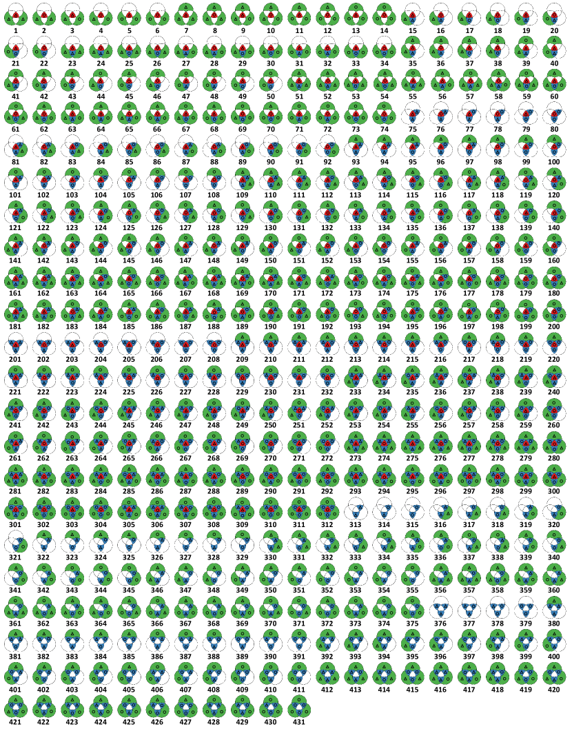
Figure 18: The 431 3H-motifs studied in this work. In each Venn diagram, uncolored regions are empty without containing any nodes. Colored regions with a triangle contain more than $0$ and at most $\theta$ nodes, while colored regions with a circle contain more than $\theta$ nodes.

In this section, we explore potential variations of 3h-motifs and assess their performance through experiments. We aim to show that the proposed 3h-motifs strike a balance between simplicity and strong characterization power, making them an effective tool for analyzing hypergraph structures. Visual representations of all 431 3h-motifs are provided in Figure 18. We consider the following variants in which the two states of each non-empty set are defined differently:

• Absolute - Abs($\theta$): The states of each non-empty set are defined based on its cardinality $c$ as (1) $0<c\leq\theta$ and (2) $c>\theta$, where $\theta=1$. Note that 3h-motifs are equivalent to Abs($1$).
  

• Motif Ratio - MR($p$): The states of each non-empty set are defined based on its cardinality $c$ and the total number of unique nodes $n$ in the considered instance as (1) $0<\frac{c}{n}\leq p$ and (2) $\frac{c}{n}>p$, where $0<p<1$.
  

• Hyperedge Ratio - HR($p,\sigma$): The states of each non-empty set are defined based on its cardinality $c$ and the hyperedges $S$ containing the set as (1) $0<\sigma((\frac{c}{|e|})_{e\in S})\leq p$ and (2) $\sigma((\frac{c}{|e|})_{e\in S})>p$, where $0<p<1$ and $\sigma(\cdot)$ is the mean, max, or min function.
  

We conduct experiments to compare the effectiveness of 3H-motifs (i.e., Abs($1$)), Abs($2$), MR($p$), HR($p$, mean), HR($p$, max), HR($p$, min) for $p=\{0.1,0.2,\cdots,0.9\}$. We evaluate the variants through hypergraph clustering, hyperedge prediction, and node classification using the same experimental settings described in Sections 6.4 and 6.5. For hyperedge prediction task is performed on the coauth-DBLP dataset.

Table 12 presents the results of comparing the performances. For MR($p$), HR($p$, mean), HR($p$, max), and HR($p$, min), the table reports the min, average, and max performances over $p=\{0.1,0.2,\cdots,0.9\}$. Remarkably, even though the definition of 3h-motifs is simplest, the use of 3h-motifs leads to the best performance in hypergraph clustering and node classification tasks. In hyperedge prediction, using 3h-motifs achieves the highest ACC and the second-highest AUC. These results provide support for the effectiveness of 3h-motifs.

We further investigate a wider range of $\theta$ value (spec., from $1$ to $15$) in Abs($\theta$) to assess its impact on performance in the considered tasks. As shown in Figure 15, our empirical findings reveal that employing a threshold of $1$ (i.e., utilizing 3h-motifs) consistently results in the highest performance across the tasks. Especially, as shown in Figure 15(d), with $\theta$ fixed at $1$, the hyperedge prediction performance remains very close to that achieved with the optimal $\theta$ value for each dataset. In Appendix M, we provide additional analysis regarding the effectiveness of employing $\theta=1$.

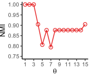
(a) Hypergraph clustering performance (NMI) w.r.t. $\theta$

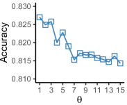
(b) Average hyperedge prediction accuracy w.r.t. $\theta$

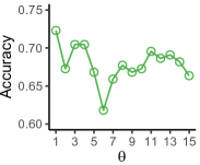
(c) Node classification accuracy w.r.t. $\theta$

(d) Average hyperedge prediction accuracy (optimal $\theta$ vs fixed $\theta$)

Figure 15: 3H-motifs (i.e., Abs($1$)) consistently demonstrates superior performance in all three applications compared to Abs($\theta$) with other $\theta$ values. In (b), we report the hyperedge prediction accuracy averaged over all datasets. In (d), $\theta^{*}$ (red bar) represents the average hyperedge prediction accuracy achieved with the optimal $\theta$ value for each dataset, while $\theta=1$ (blue bar) represents the average hyperedge prediction accuracy with $\theta$ fixed at $1$. Remarkably, even with $\theta$ fixed at $1$, the performance remains very close to the highest accuracy attainable.

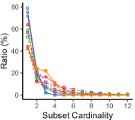
(a) Subset Cardinality Distribution

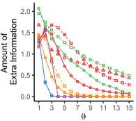
(b) Amount of Extra Information w.r.t. $\theta$

Figure 16: (a) The cardinalities of subsets, upon which both h-motifs and 3h-motifs are defined, exhibit a strong bias toward the value $1$ in all datasets. (b) The amount of extra information gained with 3h-motifs over h-motifs is maximized when utilizing the cardinality threshold $\theta=1$, as employed by 3h-motifs, in 7 out of 11 hypergraphs.

Appendix M Data Analysis Regarding the Effectiveness of 3H-motifs

In this section, we present data analyses for gaining insights into the effectiveness of 3h-motifs, which is demonstrated by comprehensive experiments in Appendix L. Recall that 3h-motifs employs a threshold value of $\theta=1$ to categorize the states of the seven subsets into three distinct groups based on their cardinalities. Our analyses below demonstrate why choosing $\theta=1$ is a suitable decision.

Subset Cardinality Distribution: We first investigate the cardinalities of the seven subsets, based on which h-motifs and 3h-motifs are defined, in the 11 real-world hypergraphs. As shown in Figure 16(a), in all considered real-world hypergraphs, the count of subsets with each cardinality diminishes considerably as the cardinality increases. This observation suggests that when employing a threshold value $\theta$ greater than $1$, only a very small fraction of subsets falls into the state $>\theta$, which is a new state introduced in 3h-motifs but not present in h-motifs. Intuitively, this limited utilization of this new state leads to a reduction in the amount of additional information provided by 3h-motifs in comparison to h-motifs.

Amount of Extra Information: To numerically validate our intuition above, we measure the amount of extra information in 3h-motifs over h-motifs using the conditional entropy as follows:

$$H(\text{3h-motif}|\text{h-motif})=-\sum_{i=1}^{26}\frac{N_{i}}{N_{tot}}\sum_{j\in K_{i}}\frac{n_{j}}{N_{i}}\ln{\frac{n_{j}}{N_{i}}},$$ (24)

where $N_{tot}$ is the count of all h-motif instances, $N_{i}$ is the count of the instances of h-motif $i$, $K_{i}$ is the set of the indices of 3h-motifs that can share instances with h-motif $i$ (e.g. $K_{1}=\{\text{1,\ldots,6}\}$, as shown in Figure 5), and $n_{j}$ is the count of the instances of 3h-motif $j$. If we treat the h-motif and 3h-motif corresponding to each instance as random variables, the conditional entropy measures the amount of information needed to describe the corresponding 3h-motif given the corresponding h-motif. If the instances of each h-motif are uniformly distributed among the corresponding 3h-motifs, we can achieve the maximum amount of additional information, which is $\sum_{i=1}^{26}\frac{N_{i}}{N_{\text{tot}}}\ln{|K_{i}|}$. Conversely, if the instance counts of h-motif $i$ are highly skewed toward one of the corresponding 3h-motifs, the extra information would approach zero, indicating a minimum. In Figure 16(b), we report the amount of extra information in each real-world hypergraph while varying $\theta$ from $1$ to $15$. In all datasets, the most significant additional information is obtained with a small $\theta$, with 7 out of 11 hypergraphs yielding the highest amount at $\theta=1$. This potentially explains the superior performance observed in machine tasks when $\theta=1$ (see Figure 15).

References

- [1] The On-Line Encyclopedia of Integer Sequences. Sequence A000612.
- [2] The On-Line Encyclopedia of Integer Sequences. Sequence A323819.
- [3] S. Agarwal, J. Lim, L. Zelnik-Manor, P. Perona, D. Kriegman, and S. Belongie. Beyond pairwise clustering. In CVPR, 2005.
- [4] N. K. Ahmed, N. Duffield, T. L. Willke, and R. A. Rossi. On sampling from massive graph streams. PVLDB, 10(11):1430–1441, 2017.
- [5] N. K. Ahmed, J. Neville, R. A. Rossi, and N. Duffield. Efficient graphlet counting for large networks. In ICDM, 2015.
- [6] N. K. Ahmed, J. Neville, R. A. Rossi, N. G. Duffield, and T. L. Willke. Graphlet decomposition: Framework, algorithms, and applications. KAIS, 50(3):689–722, 2017.
- [7] S. G. Aksoy, T. G. Kolda, and A. Pinar. Measuring and modeling bipartite graphs with community structure. Journal of Complex Networks, 5(4):581–603, 2017.
- [8] N. Alon, R. Yuster, and U. Zwick. Color-coding. JACM, 42(4):844–856, 1995.
- [9] I. Amburg, N. Veldt, and A. R. Benson. Hypergraph clustering with categorical edge labels. In WWW, 2020.
- [10] A. Antelmi, G. Cordasco, M. Polato, V. Scarano, C. Spagnuolo, and D. Yang. A survey on hypergraph representation learning. ACM Computing Surveys, 56(1):1–38, 2023.
- [11] C. Aslay, M. A. U. Nasir, G. De Francisci Morales, and A. Gionis. Mining frequent patterns in evolving graphs. In CIKM, 2018.
- [12] A.-L. Barabási and R. Albert. Emergence of scaling in random networks. Science, 286(5439):509–512, 1999.
- [13] L. Becchetti, P. Boldi, C. Castillo, and A. Gionis. Efficient algorithms for large-scale local triangle counting. TKDD, 4(3):1–28, 2010.
- [14] A. R. Benson, R. Abebe, M. T. Schaub, A. Jadbabaie, and J. Kleinberg. Simplicial closure and higher-order link prediction. PNAS, 115(48):E11221–E11230, 2018.
- [15] A. R. Benson, D. F. Gleich, and J. Leskovec. Higher-order organization of complex networks. Science, 353(6295):163–166, 2016.
- [16] A. R. Benson, R. Kumar, and A. Tomkins. Sequences of sets. In KDD, 2018.
- [17] M. A. Bhuiyan, M. Rahman, M. Rahman, and M. Al Hasan. Guise: Uniform sampling of graphlets for large graph analysis. In ICDM, 2012.
- [18] S. P. Borgatti and M. G. Everett. Network analysis of 2-mode data. Social networks, 19(3):243–270, 1997.
- [19] M. Bressan, F. Chierichetti, R. Kumar, S. Leucci, and A. Panconesi. Counting graphlets: Space vs time. In WSDM, 2017.
- [20] M. Bressan, S. Leucci, and A. Panconesi. Motivo: fast motif counting via succinct color coding and adaptive sampling. PVLDB, 12(11):1651–1663, 2019.
- [21] M. Bressan, S. Leucci, and A. Panconesi. Faster motif counting via succinct color coding and adaptive sampling. TKDD, 15(6):1–27, 2021.
- [22] F. Bu, G. Lee, and K. Shin. Hypercore decomposition for non-fragile hyperedges: Concepts, algorithms, observations, and applications. arXiv preprint arXiv:2301.08440, 2023.
- [23] J. Bu, S. Tan, C. Chen, C. Wang, H. Wu, L. Zhang, and X. He. Music recommendation by unified hypergraph: combining social media information and music content. In MM, 2010.
- [24] G. Cencetti, F. Battiston, B. Lepri, and M. Karsai. Temporal properties of higher-order interactions in social networks. Scientific reports, 11(1):7028, 2021.
- [25] L. Chen, X. Qu, M. Cao, Y. Zhou, W. Li, B. Liang, W. Li, W. He, C. Feng, X. Jia, et al. Identification of breast cancer patients based on human signaling network motifs. Scientific reports, 3:3368, 2013.
- [26] T. Chen and C. Guestrin. Xgboost: A scalable tree boosting system. In KDD, 2016.
- [27] X. Chen, Y. Li, P. Wang, and J. C. Lui. A general framework for estimating graphlet statistics via random walk. PVLDB, 10(3):253–264, 2016.
- [28] M. Choe, S. Kim, J. Yoo, and K. Shin. Classification of edge-dependent labels of nodes in hypergraphs. In KDD, 2023.
- [29] H. Choo and K. Shin. On the persistence of higher-order interactions in real-world hypergraphs. In SDM, 2022.
- [30] C. Comrie and J. Kleinberg. Hypergraph ego-networks and their temporal evolution. In ICDM, 2021.
- [31] Z. Cui, Y. Cai, S. Wu, X. Ma, and L. Wang. Motif-aware sequential recommendation. In SIGIR, 2021.
- [32] L. De Stefani, A. Epasto, M. Riondato, and E. Upfal. Trièst: Counting local and global triangles in fully-dynamic streams with fixed memory size. In KDD, 2016.
- [33] M. T. Do, S.-e. Yoon, B. Hooi, and K. Shin. Structural patterns and generative models of real-world hypergraphs. In KDD, 2020.
- [34] M. Faloutsos, P. Faloutsos, and C. Faloutsos. On power-law relationships of the internet topology. ACM SIGCOMM computer communication review, 29(4):251–262, 1999.
- [35] S. R. Gallagher and D. S. Goldberg. Clustering coefficients in protein interaction hypernetworks. In BCB, 2013.
- [36] P. Gupta, V. Satuluri, A. Grewal, S. Gurumurthy, V. Zhabiuk, Q. Li, and J. Lin. Real-time twitter recommendation: Online motif detection in large dynamic graphs. VLDB, 7(13):1379–1380, 2014.
- [37] G. Han and H. Sethu. Waddling random walk: Fast and accurate mining of motif statistics in large graphs. In ICDM, 2016.
- [38] W. Hoeffding. Probability inequalities for sums of bounded random variables. The collected works of Wassily Hoeffding, pages 409–426, 1994.
- [39] P. W. Holland and S. Leinhardt. A method for detecting structure in sociometric data. In Social Networks, pages 411–432. Elsevier, 1977.
- [40] S. Hu, X. Wu, and T. H. Chan. Maintaining densest subsets efficiently in evolving hypergraphs. In CIKM, 2017.
- [41] X. Hu, Y. Tao, and C.-W. Chung. Massive graph triangulation. In SIGMOD, 2013.
- [42] X. Hu, Y. Tao, and C.-W. Chung. I/o-efficient algorithms on triangle listing and counting. TODS, 39(4):1–30, 2014.
- [43] Y. Huang, Q. Liu, S. Zhang, and D. N. Metaxas. Image retrieval via probabilistic hypergraph ranking. In CVPR, 2010.
- [44] H. Hwang, S. Lee, C. Park, and K. Shin. Ahp: Learning to negative sample for hyperedge prediction. In SIGIR, 2022.
- [45] T. Hwang, Z. Tian, R. Kuangy, and J.-P. Kocher. Learning on weighted hypergraphs to integrate protein interactions and gene expressions for cancer outcome prediction. In ICDM, 2008.
- [46] U. Jeong, K. Ding, L. Cheng, R. Guo, K. Shu, and H. Liu. Nothing stands alone: Relational fake news detection with hypergraph neural networks. In Big Data, 2022.
- [47] M. Jha, C. Seshadhri, and A. Pinar. A space efficient streaming algorithm for triangle counting using the birthday paradox. In KDD, 2013.
- [48] J. Jiang, Y. Wei, Y. Feng, J. Cao, and Y. Gao. Dynamic hypergraph neural networks. In IJCAI, 2019.
- [49] U. Kang, C. E. Tsourakakis, A. P. Appel, C. Faloutsos, and J. Leskovec. Radius plots for mining tera-byte scale graphs: Algorithms, patterns, and observations. In SDM, 2010.
- [50] G. Karypis, R. Aggarwal, V. Kumar, and S. Shekhar. Multilevel hypergraph partitioning: applications in vlsi domain. TVLSI, 7(1):69–79, 1999.
- [51] G. Karypis and V. Kumar. Multilevel k-way hypergraph partitioning. VLSI design, 11(3):285–300, 2000.
- [52] H. Kim, J. Ko, F. Bu, and K. Shin. Characterization of simplicial complexes by counting simplets beyond four nodes. In WWW, 2023.
- [53] J. Kim, W.-S. Han, S. Lee, K. Park, and H. Yu. Opt: a new framework for overlapped and parallel triangulation in large-scale graphs. In SIGMOD, 2014.
- [54] S. Kim, M. Choe, J. Yoo, and K. Shin. Reciprocity in directed hypergraphs: Measures, findings, and generators. In ICDM, 2022.
- [55] B. Klimt and Y. Yang. The enron corpus: A new dataset for email classification research. In ECML PKDD, 2004.
- [56] J. Ko, Y. Kook, and K. Shin. Growth patterns and models of real-world hypergraphs. KAIS, 64(11):2883–2920, 2022.
- [57] S. Ko and W.-S. Han. Turbograph++ a scalable and fast graph analytics system. In SIGMOD, 2018.
- [58] M. Latapy, C. Magnien, and N. Del Vecchio. Basic notions for the analysis of large two-mode networks. Social networks, 30(1):31–48, 2008.
- [59] D. Lee and K. Shin. I’m me, we’re us, and i’m us: Tri-directional contrastive learning on hypergraphs. In AAAI, 2023.
- [60] G. Lee, M. Choe, and K. Shin. How do hyperedges overlap in real-world hypergraphs?-patterns, measures, and generators. In WWW, 2021.
- [61] G. Lee, M. Choe, and K. Shin. Hashnwalk: Hash and random walk based anomaly detection in hyperedge streams. In IJCAI, 2022.
- [62] G. Lee, J. Ko, and K. Shin. Hypergraph motifs: concepts, algorithms, and discoveries. PVLDB, 13(12):2256–2269, 2020.
- [63] G. Lee and K. Shin. Thyme+: Temporal hypergraph motifs and fast algorithms for exact counting. In ICDM, 2021.
- [64] G. Lee and K. Shin. Temporal hypergraph motifs. KAIS, 65(4):1549–1586, 2023.
- [65] J. B. Lee, R. A. Rossi, X. Kong, S. Kim, E. Koh, and A. Rao. Graph convolutional networks with motif-based attention. In CIKM, 2019.
- [66] J. Leskovec, J. Kleinberg, and C. Faloutsos. Graphs over time: densification laws, shrinking diameters and possible explanations. In KDD, 2005.
- [67] J. Leskovec and R. Sosič. Snap: A general-purpose network analysis and graph-mining library. TIST, 8(1):1, 2016.
- [68] D. Li, Z. Xu, S. Li, and X. Sun. Link prediction in social networks based on hypergraph. In WWW, 2013.
- [69] L. Li and T. Li. News recommendation via hypergraph learning: encapsulation of user behavior and news content. In WSDM, 2013.
- [70] M. Li, Y. Zhang, X. Li, L. Cai, and B. Yin. Multi-view hypergraph neural networks for student academic performance prediction. Engineering Applications of Artificial Intelligence, 114:105174, 2022.
- [71] P.-Z. Li, L. Huang, C.-D. Wang, and J.-H. Lai. Edmot: An edge enhancement approach for motif-aware community detection. In KDD, 2019.
- [72] Y. Li, H. Chen, X. Sun, Z. Sun, L. Li, L. Cui, P. S. Yu, and G. Xu. Hyperbolic hypergraphs for sequential recommendation. In CIKM, 2021.
- [73] Z. Liu, X. Xie, and L. Chen. Context-aware academic collaborator recommendation. In KDD, 2018.
- [74] H.-W. Ma, B. Kumar, U. Ditges, F. Gunzer, J. Buer, and A.-P. Zeng. An extended transcriptional regulatory network of escherichia coli and analysis of its hierarchical structure and network motifs. Nucleic acids research, 32(22):6643–6649, 2004.
- [75] R. Mastrandrea, J. Fournet, and A. Barrat. Contact patterns in a high school: a comparison between data collected using wearable sensors, contact diaries and friendship surveys. PloS one, 10(9), 2015.
- [76] R. Matsuno and A. Gionis. Improved mixing time for k-subgraph sampling. In SDM, 2020.
- [77] T. Mikolov, I. Sutskever, K. Chen, G. S. Corrado, and J. Dean. Distributed representations of words and phrases and their compositionality. In NIPS, 2013.
- [78] R. Milo, S. Itzkovitz, N. Kashtan, R. Levitt, S. Shen-Orr, I. Ayzenshtat, M. Sheffer, and U. Alon. Superfamilies of evolved and designed networks. Science, 303(5663):1538–1542, 2004.
- [79] R. Milo, S. Shen-Orr, S. Itzkovitz, N. Kashtan, D. Chklovskii, and U. Alon. Network motifs: simple building blocks of complex networks. Science, 298(5594):824–827, 2002.
- [80] D. A. Nguyen, C. H. Nguyen, P. Petschner, and H. Mamitsuka. Sparse: a sparse hypergraph neural network for learning multiple types of latent combinations to accurately predict drug–drug interactions. Bioinformatics, 38:i333–i341, 2022.
- [81] C. C. Noble and D. J. Cook. Graph-based anomaly detection. In KDD, 2003.
- [82] M. Ouyang, M. Toulouse, K. Thulasiraman, F. Glover, and J. S. Deogun. Multilevel cooperative search for the circuit/hypergraph partitioning problem. TCAD, 21(6):685–693, 2002.
- [83] R. Pagh and C. E. Tsourakakis. Colorful triangle counting and a mapreduce implementation. Information Processing Letters, 112(7):277–281, 2012.
- [84] C. R. Palmer, P. B. Gibbons, and C. Faloutsos. Anf: A fast and scalable tool for data mining in massive graphs. In KDD, 2002.
- [85] A. Paranjape, A. R. Benson, and J. Leskovec. Motifs in temporal networks. In WSDM, 2017.
- [86] F. Pedregosa, G. Varoquaux, A. Gramfort, V. Michel, B. Thirion, O. Grisel, M. Blondel, P. Prettenhofer, R. Weiss, V. Dubourg, J. Vanderplas, A. Passos, D. Cournapeau, M. Brucher, M. Perrot, and E. Duchesnay. Scikit-learn: Machine learning in Python. JMLR, 12:2825–2830, 2011.
- [87] A. Pinar, C. Seshadhri, and V. Vishal. Escape: Efficiently counting all 5-vertex subgraphs. In WWW, 2017.
- [88] G. Preti, G. De Francisci Morales, and F. Bonchi. Fresco: Mining frequent patterns in simplicial complexes. In WWW, 2022.
- [89] R. A. Rossi, N. K. Ahmed, A. Carranza, D. Arbour, A. Rao, S. Kim, and E. Koh. Heterogeneous network motifs. arXiv preprint arXiv:1901.10026, 2019.
- [90] R. A. Rossi, N. K. Ahmed, and E. Koh. Higher-order network representation learning. In WWW Companion, 2018.
- [91] T. K. Saha and M. Al Hasan. Finding network motifs using mcmc sampling. In Complex Networks VI, pages 13–24. Springer, 2015.
- [92] S.-V. Sanei-Mehri, A. E. Sariyuce, and S. Tirthapura. Butterfly counting in bipartite networks. In KDD, 2018.
- [93] A. Sankar, X. Zhang, and K. C.-C. Chang. Motif-based convolutional neural network on graphs. arXiv preprint arXiv:1711.05697, 2017.
- [94] S. S. Shen-Orr, R. Milo, S. Mangan, and U. Alon. Network motifs in the transcriptional regulation network of escherichia coli. Nature genetics, 31(1):64–68, 2002.
- [95] K. Shin. Wrs: Waiting room sampling for accurate triangle counting in real graph streams. In ICDM, 2017.
- [96] K. Shin, S. Oh, J. Kim, B. Hooi, and C. Faloutsos. Fast, accurate and provable triangle counting in fully dynamic graph streams. TKDD, 14(2):1–39, 2020.
- [97] A. Sinha, Z. Shen, Y. Song, H. Ma, D. Eide, B.-J. Hsu, and K. Wang. An overview of microsoft academic service (mas) and applications. In WWW, 2015.
- [98] N. Sloane. The On-Line Encyclopedia of Integer Sequences.
- [99] J. Stehlé, N. Voirin, A. Barrat, C. Cattuto, L. Isella, J.-F. Pinton, M. Quaggiotto, W. Van den Broeck, C. Régis, B. Lina, et al. High-resolution measurements of face-to-face contact patterns in a primary school. PloS one, 6(8), 2011.
- [100] L. Sun, S. Ji, and J. Ye. Hypergraph spectral learning for multi-label classification. In KDD, 2008.
- [101] Y. Sun, D. Zhu, H. Du, and Z. Tian. Motifs-based recommender system via hypergraph convolution and contrastive learning. Neurocomputing, 512:323–338, 2022.
- [102] C. E. Tsourakakis, U. Kang, G. L. Miller, and C. Faloutsos. Doulion: counting triangles in massive graphs with a coin. In KDD, 2009.
- [103] C. E. Tsourakakis, J. Pachocki, and M. Mitzenmacher. Scalable motif-aware graph clustering. In WWW, 2017.
- [104] P. Wang, P. Jia, Y. Qi, Y. Sun, J. Tao, and X. Guan. Rept: A streaming algorithm of approximating global and local triangle counts in parallel. In ICDE, 2019.
- [105] P. Wang, J. C. Lui, B. Ribeiro, D. Towsley, J. Zhao, and X. Guan. Efficiently estimating motif statistics of large networks. TKDD, 9(2):1–27, 2014.
- [106] P. Wang, Y. Qi, Y. Sun, X. Zhang, J. Tao, and X. Guan. Approximately counting triangles in large graph streams including edge duplicates with a fixed memory usage. PVLDB, 11(2):162–175, 2017.
- [107] D. J. Watts and S. H. Strogatz. Collective dynamics of ‘small-world’networks. Nature, 393(6684):440, 1998.
- [108] X. Wu, Q. Chen, W. Li, Y. Xiao, and B. Hu. Adahgnn: Adaptive hypergraph neural networks for multi-label image classification. In MM, 2020.
- [109] D. Yang, B. Qu, J. Yang, and P. Cudre-Mauroux. Revisiting user mobility and social relationships in lbsns: A hypergraph embedding approach. In WWW, 2019.
- [110] E. Yeger-Lotem, S. Sattath, N. Kashtan, S. Itzkovitz, R. Milo, R. Y. Pinter, U. Alon, and H. Margalit. Network motifs in integrated cellular networks of transcription–regulation and protein–protein interaction. Proceedings of the National Academy of Sciences, 101(16):5934–5939, 2004.
- [111] H. Yin, A. R. Benson, J. Leskovec, and D. F. Gleich. Local higher-order graph clustering. In KDD, 2017.
- [112] S.-e. Yoon, H. Song, K. Shin, and Y. Yi. How much and when do we need higher-order information in hypergraphs? a case study on hyperedge prediction. In WWW, 2020.
- [113] J. Yu, D. Tao, and M. Wang. Adaptive hypergraph learning and its application in image classification. TIP, 21(7):3262–3272, 2012.
- [114] Y. Yu, Z. Lu, J. Liu, G. Zhao, and J.-r. Wen. Rum: Network representation learning using motifs. In ICDE, 2019.
- [115] Z. Yu and H. Gao. Molecular representation learning via heterogeneous motif graph neural networks. In ICML, 2022.
- [116] X. Yuan, N. Zhou, S. Yu, H. Huang, Z. Chen, and F. Xia. Higher-order structure based anomaly detection on attributed networks. In Big Data, 2021.
- [117] M. Zhang, Z. Cui, S. Jiang, and Y. Chen. Beyond link prediction: Predicting hyperlinks in adjacency space. In AAAI, 2018.
- [118] X. Zhang, L. Xu, and Z. Xu. Influence maximization based on network motifs in mobile social networks. IEEE Transactions on Network Science and Engineering, 9(4):2353–2363, 2022.
- [119] H. Zhao, X. Xu, Y. Song, D. L. Lee, Z. Chen, and H. Gao. Ranking users in social networks with higher-order structures. In AAAI, 2018.
- [120] H. Zhao, Y. Zhou, Y. Song, and D. L. Lee. Motif enhanced recommendation over heterogeneous information network. In CIKM, 2019.
- [121] D. Zhou, J. Huang, and B. Schölkopf. Learning with hypergraphs: Clustering, classification, and embedding. In NIPS, 2007.