Decentralized Proximal Method of Multipliers for Convex Optimization with Coupled Constraints

Abstract

In this paper, a decentralized proximal method of multipliers (DPMM) is proposed to solve constrained convex optimization problems over multi-agent networks, where the local objective of each agent is a general closed convex function, and the constraints are coupled equalities and inequalities. This algorithm strategically integrates the dual decomposition method and the proximal point algorithm. One advantage of DPMM is that subproblems can be solved inexactly and in parallel by agents at each iteration, which relaxes the restriction of requiring exact solutions to subproblems in many distributed constrained optimization algorithms. We show that the first-order optimality residual of the proposed algorithm decays to $0$ at a rate of $o(1/k)$ under general convexity. Furthermore, if a structural assumption for the considered optimization problem is satisfied, the sequence generated by DPMM converges linearly to an optimal solution. In numerical simulations, we compare DPMM with several existing algorithms using two examples to demonstrate its effectiveness.

Keywords: Distributed convex optimization, optimization algorithm, sublinear convergence rate, linear convergence rate.

1 Introduction

Distributed optimization algorithms decompose an optimization problem into smaller, more manageable subproblems that can be solved in parallel by a group of agents or processors. All agents communicate peer-to-peer and compute locally, cooperating to minimize the global objective function. Consequently, distributed optimization algorithms are widely used to solve large-scale problems in wireless communication, optimal control, machine learning, etc. Many problems of interest can be formulated as the following distributed constrained optimization model

$$\min_{\mathrm{x}}F(\mathrm{x})\triangleq\sum_{i=1}^{m}f_{i}(\mathrm{x}_{i})$$ (P)

$${\rm s.t.} \sum_{i=1}^{m}\underbrace{\left[\begin{array}[]{c}A_{i}\mathrm{x}_{i}-b_{i}\\ g_{i}(\mathrm{x}_{i})\end{array}\right]}_{\triangleq\ G_{i}(\mathrm{x}_{i})}\in\underbrace{\left[\begin{array}[]{c}0_{p}\\ \mathbb{R}^{q}_{-}\end{array}\right]}_{\triangleq\ \mathcal{K}},$$

$$\mathrm{x}_{i}\in\Omega_{i},\ i=1,2,\dots,m,$$

where $\mathrm{x}_{i}\in\mathbb{R}^{n_{i}}$ is the local decision variable controlled by agent $i$, $\mathrm{x}=\mathrm{col}(\mathrm{x}_{1},\mathrm{x}_{2},\dots,\mathrm{x}_{m})\in\mathbb{R}^{n}$, $n=\sum_{i=1}^{m}n_{i}$. The objective $f_{i}:\mathbb{R}^{n_{i}}\to\mathbb{R}$, constraint function $h_{i}:\mathbb{R}^{n_{i}}\to\mathbb{R}^{q}$, $A_{i}\in\mathbb{R}^{p\times n_{i}}$, $b_{i}\in\mathbb{R}^{p}$, and local constraint subset $\Omega_{i}\subseteq\mathbb{R}^{n_{i}}$. The local information $\mathcal{F}_{i}=\left\{f_{i},A_{i},b_{i},h_{i},\Omega_{i}\right\}$ can only be known by agent $i$, but none of the other agents have access to this information. We aim to develop a distributed algorithm to solve (P), which means that all agents can only access and process local data, and communicate only with their immediate neighbors. Through exchanging information, they cooperate to find an optimal solution to (P).

Various distributed algorithms have been proposed to solve optimization problems with coupled constraints. The coupled linear equality constrained optimization problems were widely studied at first and probably inspired by distributed resource allocation problems (e.g., [1, 2]). The augmented Lagrangian method (ALM) and the alternating direction method of multipliers (ADMM) are classical and efficient algorithms for equality constrained convex optimization problems in centralized environments. These two algorithms are extended to solve distributed optimization problems with coupled linear constraints. To name a few, Tracking-ADMM [3], Non-Ergodic Consensus-Based Primal-Dual Algorithm [4] (NECPD), Consensus-Based Distributed Augmented Lagrangian Method [5] (C-ADAL), Primal-Dual Consensus ADMM [6] (PDC-ADMM). Among the above listed algorithms, Tracking-ADMM is asymptotically convergent, while NECPD, C-ADAL, and PDC-ADMM all have $O(1/k)$ convergence rates, in terms of the objective residual and feasibility. The first-order optimality residual of Mirror-P-EXTRA proposed by [1] decays to $0$ at a rate of $o(1/k)$.

Existing methods for tackling coupled nonlinear inequality constraints can be classified into two categories: primal decomposition and dual decomposition. The primal decomposition method introduces artificial variables to transform the coupled inequality constraints into a more manageable form. For instance, the authors of [7] transformed the coupled inequality constrained convex optimization into a bi-level convex programming problem. Their proposed distributed primal-dual algorithm has a convergence rate of $O(1/\log(k))$ for the objective residuals. Similarly, the authors of [8] employed artificial variables to decouple the inequality constraints, at the cost of adding a coupled linear equality constraint working on the auxiliary variables. Their IPLUX algorithm achieves a convergence rate of $O(1/k)$ in terms of feasibility and optimality. On the other hand, the dual decomposition method utilizes Lagrange duality to establish a consensus-based dual problem. Various distributed consensus-based algorithms can then be integrated to solve the dual problem. For example, the distributed dual subgradient algorithm proposed by [9, 10] has an ergodic $O(1/k)$ convergence rate. The authors of [11] integrated the dual gradient tracking method (see [12]) and a primal recovery technique to develop a primal-dual algorithm with objective residuals decaying to $0$ at a rate of $O(1/k)$. The work of [13] focused on smooth convex optimization problems and proposed a distributed algorithm that performs two successive gradient projection steps in each round of iteration for a min-max problem formulated by the dual decomposition. They showed that their algorithm with a small fixed stepsize asymptotically converges to a saddle point. Recently, the authors of [14] proposed an augmented Lagrangian tracking (AL-tracking) method, and they demonstrated that any cluster of the primal decision sequences generated by the AL-tracking algorithm is an optimal solution.

Table 1: An overview of some existing distributed coupled constrained optimization algorithms.

   The full names of the abbreviations in this table are listed there: C (convex), SC (strongly convex), NSO (non-smooth optimization), E (equality), I (inequality (probably nonlinear)), OR (objective residual), FR (feasibility residual), FOOR (first-order optimality residual).

Algorithms	NSO	Communications	Coupled constraints		Convergence of $\{\mathrm{x}^{k}\}_{k=0}^{\infty}$ $\dagger$	Convergence rate
			E	I		C		SC
NECPD [4]	$\surd$	$(d-1)$$\dagger\dagger$	$\surd$	$\times$	—	OR & FR	$O(1/k)$	—
Tracking- ADMM [3]	$\surd$	1	$\surd$	$\times$	$\times$	—
AL-Tracking [14]	$\surd$	1	$\surd$	$\surd$	$\times$	—
PDC- ADMM [6]	$\surd$	2	$\surd$	$\times$	$\surd$	OR & FR	$O(1/k)$	—
[13]	$\times$	2	$\surd$	$\surd$	$\surd$	—
IPLUX [8]	$\surd$	2	$\surd$	$\surd$	—	OR & FR	$O(1/k)$	—
[2] $\dagger\dagger\dagger$	$\times$	1	$\surd$	$\times$	$\surd$	—		linear
Mirror- P-EXTRA [1]	$\surd$	1	$\surd$	$\times$	$\surd$	FOOR	$o(1/k)$	linear
This paper	$\surd$	1	$\surd$	$\surd$	$\surd$	FOOR	$o(1/k)$	linear

• $\{\mathrm{x}^{k}\}_{k=0}^{\infty}$ is the decision variable sequence of agents, generated by each algorithm in this table.

• $d$ is the degree of the minimal polynomial of the adjacency matrix $W$.

• The algorithm of [2] can be applied to time-varying directed graphs, and other algorithms in this table employ a fixed undirected graph.

In this paper, we will apply the dual decomposition method twice successively to handle coupled constraints and the consensus dual problem, to construct a Karush-Kuhn-Tucker (KKT) system of (P) that is separable with respect to the primal decision variables and the Lagrange multipliers respectively. This KKT system would be treated as an inclusion problem of a maximal monotone operator that can employ the proximal point method – an efficient algorithm in a centralized environment, to solve it. By strategically integrating ideas from the variable metric proximal point method and the prediction-correction framework presented by [15], we propose a decentralized proximal method of multipliers (DPMM) for this monotone inclusion problem, which is also a distributed algorithm for (P).

In the DPMM algorithm, each agent controls three variables: the primal decision variable, a local estimate (copy) of the Lagrange multiplier corresponding to the coupled constraints, and an introduced auxiliary variable. The local estimates of the Lagrange multiplier enable the algorithm to be executed in a distributed fashion, while the auxiliary variables push agents’ local estimates to be consensual. During each round of iteration, all agents communicate with neighbors for only one round, exchanging only the values of agents’ local estimates of the Lagrange multiplier. The contribution of this work to the research of distributed constrained optimization is four-fold.

1. The decentralized proximal method of multipliers proposed in this article solves a challenging family of constrained convex optimization problems, where constraints (including equality and nonlinear inequalities) are coupled, the objective and constraint functions can be general closed convex (probably non-smooth), and the local constraint sets of agents are closed convex and not required to be bounded. The assumptions of a bounded feasible region and smooth objective and constraint functions, either of which is an indispensable condition for many distributed constrained optimization algorithms to guarantee convergence, e.g., [5, 6, 11, 3, 9, 4, 7, 13];

2. DPMM is a primal-dual convergent method. The sequences of primal decision variables and Lagrange multipliers generated by DPMM converge to a primal-optimal and dual-optimal solution, respectively. In contrast, some algorithms in the literature have only dual convergence, while the convergence of their generated primal decision sequence is either unknown (e.g., [11, 7, 5, 8]) or each cluster is a primal optimal solution (e.g., [9, 3, 14]). In addition, as shown in Table 1, DPMM has a lower communication burden compared with some other existing algorithms.

3. In this paper, an inexact version of the decentralized proximal method of multipliers (inexact-DPMM) is presented to relax the restriction that the minimization subproblems are solved exactly by agents at each iteration (e.g., [8, 3, 9, 4, 5, 13, 11]). Inexact-DPMM is still convergent to an optimal solution of (P), and if the precision of minimizing subproblem geometrically decays to $0$, its first-order optimality residual then converges to zero at a rate of $o(1/k)$.

4. Under a structural assumption that includes strong convexity of the objective function, we demonstrate that inexact-DPMM has a linear convergence rate. Many other distributed coupled constrained optimization algorithms in literature do not have results about the linear convergence rate, for a survey, see Table 1.

The rest of the paper is organized as follows: In Section 2, we state some standard assumptions about the network model of agents and the considered optimization problems, respectively. In Section 3, we utilize the dual decomposition method to reformulate the KKT system of the problem (P) and present the distributed proximal method of multipliers, including an inexact version. In Section 4, we analyze the convergence and rate of inexact-DPMM. In Section 5, we numerically simulate DPMM for solving two examples and compare it with some algorithms in Table 1 to illustrate its effectiveness. In section 6, we make a conclusion.

Notation: Let $\mathbb{R}^{n}$ be the $n$-dimensional Euclidean space with the inner product $\langle\cdot,\cdot\rangle$ and norm $\|\cdot\|$. We use $\mathbf{1}_{m}$ to denote an $m$-dimensional vector whose entries are all ones, and $I_{p}$ to denote the identity matrix with dimension $p$. The notation ${\rm col}(\mathrm{x},\mathrm{y})$ means a column vector with $\mathrm{x}$ and $\mathrm{y}$ as its components. Suppose $\Omega$ is a nonempty subset of $\mathbb{R}^{n}$. We write ${\rm int}(\Omega)$ as its interior. $\delta_{\Omega}(\mathrm{x})$ is the indicator function, which is $0$ if $\mathrm{x}\in\Omega$, and $+\infty$ otherwise. The symbol $\mathcal{P}_{\Omega}(\mathrm{x})$ stands for the projection of $\mathrm{x}$ onto $\Omega$. If $\mathcal{K}$ is a closed convex cone in $\mathbb{R}^{n}$, we denote its polar by $\mathcal{K}^{\circ}$. Let $U$ be an $n\times m$ matrix. Its transpose is denoted by $U^{\top}$. The notation $U\succ 0$ means that the matrix $U$ is symmetric positive definite. The null space of $U$, i.e., the set of all matrices $X\in\mathbb{R}^{m\times r}$ such that $UX=0$, is denoted by ${\rm null}\{U\}$. The notation ${\rm diag}(A,B)$ defines a block diagonal matrix with $A$ and $B$ as its diagonal blocks. We use $\otimes$ to denote the Kronecker product. Suppose $\mathbf{H}$ is a symmetric positive definite matrix, we define the $\mathbf{H}$-matrix norm of a vector $\mathrm{x}$ as $\|\mathrm{x}\|_{\mathbf{H}}=\sqrt{\langle\mathrm{x},\mathbf{H}\mathrm{x}\rangle}$. $\lambda_{\max}(\mathbf{H})$ and $\lambda_{\min}(\mathbf{H})$ denote the maximum and minimum eigenvalue of the matrix $\mathbf{H}$, respectively. To avoid confusion, we use the notation $\mathrm{x}^{k}$ for the value of $\mathrm{x}$ at the $k$-th iteration, and $(\mathrm{x})^{s}$ for the $s$-th power of $\mathrm{x}$.

2 Network Moldel and Assumptions

Consider a multi-agent network consisting of $m$ agents, we model it as an undirected graph $\mathcal{G}=(\mathcal{V},\mathcal{E})$, where $\mathcal{V}=\{1,2,\dots,m\}$ is the sets of nodes (i.e., agents), and $\mathcal{V}$ is the set of edges. An edge $(i,j)\in\mathcal{E}$ if and only if agent $i$ and agent $j$ can communicate and exchange information with each other. We define the index subset of neighbors of agent $i$ as $\mathcal{N}_{i}=\{j\in\mathcal{V}:(i,j)\in\mathcal{E}\}$, for all $i\in\mathcal{V}$. The adjacency matrix $W$ of the graph $\mathcal{G}$ satisfies $W_{ij}=1$, if $(i,j)\in\mathcal{E}$, and $W_{ij}=0$ otherwise. Let $\text{\L}_{\mathcal{G}}$ denote the Laplacian matrix which is compatiable with $\mathcal{G}$, i.e., $\text{\L}_{\mathcal{G}}=D-W$, where $D$ is a diagonal matrix with the entry $D_{ii}$ being the degree of agent $i$. A few facts about $\text{\L}_{\mathcal{G}}$ are that $\text{\L}_{\mathcal{G}}$ is symmetric and positive semidefinite and satisfies ${\rm null}\{\text{\L}_{\mathcal{G}}\}=\{t\mathbf{1}_{m}:t\in\mathbb{R}\}$.

In this article, we use a matrix $\text{\L}=[\text{\L}_{ij}]$ that can have more choices, which plays a role close to or the same as $\text{\L}_{\mathcal{G}}$.

   Assumption 1 (Graph connectivity).

The undirected graph $\mathcal{G}$ is connected and a matrix Ł is compatible with $\mathcal{G}$. Furthermore, $\text{\rm\L}=U^{\top}U$ for some full row-rank matrix $U$ and $U\mathbf{1}_{m}=0$.

The connectivity assumption of $\mathcal{G}$ is standard for distributed optimization. Reference [16] uses $U=\sqrt{\text{\L}}$, while we use the decomposition $\text{\L}=U^{\top}U$. The null properties of Ł and $U$ in Assumption 1 imply that ${\rm null}\{\text{\L}\}={\rm null}\{U\}$. Let

$$\textbf{\L}\triangleq\text{\L}\otimes I_{p+q}\ ,\quad\mathbf{U}\triangleq U\otimes I_{p+q}\ .$$ (2.1)

Thus we have

$$\mathrm{y}_{1}=\mathrm{y}_{2}=\cdots=\mathrm{y}_{m}\Longleftrightarrow\textbf{\L}\mathrm{Y}=0\Longleftrightarrow\mathbf{U}\mathrm{Y}=0,$$ (2.2)

where $\mathrm{Y}=\mathrm{col}\left(\mathrm{y}_{1},\mathrm{y}_{2},\dots,\mathrm{y}_{m}\right)\in\mathbb{R}^{m(p+q)}$. Relation (2.2) is a common technique for distributed algorithms that employ the dual decomposition method, and it plays a key role in extending many centralized algorithms to distributed settings.

   Remark 1.

The matrix Ł can be chosen in several different ways:

1. Since the Laplacian matrix $\text{\rm\L}_{\mathcal{G}}$ satisfies Assumption 1, we can choose $\text{\rm\L}=\text{\rm\L}_{\mathcal{G}}$. In this case, each agent needs to know the number of its neighbors (its degree) and Ł can be constructed without any communication among the agents.

2. We can choose $\text{\rm\L}=(I-W)/\nu$ [17, 18, 19], where $\nu>0$ is a scaling parameter, and $W$ is a symmetric doubly stochastic matrix that is compatible with $\mathcal{G}$. This matrix can be constructed using some local strategies such as the Metropolis-Hasting rule [20].

   Assumption 2 (Convexity and existence of optimal solution).

1. (P) is a convex problem, i.e., each $f_{i}$ and $h_{i}$ (vector-valued) are general proper closed convex functions (probably non-smooth), and each $\Omega_{i}$ is an empty closed convex subset in $\mathbb{R}^{n_{i}}$, for all $i=1,2,\dots,m$.

2. The optimal solution set $\mathcal{X}^{*}$ of (P) is nonempty.

Note that we do not require the boundedness of the local constraint subsets $\Omega_{i}$, $i=1,2,\dots,m$. However, many distributed constrained optimization algorithms in the literature rely on the boundedness (or compactness) of $\Omega_{i}$’s to bound the (sub)gradients $\nabla f_{i}$ (or $\partial f_{i}$) and the primal decision sequence $\{\mathrm{x}^{k}\}_{k\geq 0}$ that they generate.

Let $\mathcal{K}^{\circ}=\mathbb{R}^{p}\times\mathbb{R}^{q}_{+}$, the Lagrange dual problem of (P) is then formulated as

$$\max_{\mathrm{y}\in{\mathbb{R}^{p+q}}}\varphi(\mathrm{y})\triangleq\sum_{i=1}^{m}\varphi_{i}(\mathrm{y}),$$ (D)

where

$$\varphi_{i}(\mathrm{y}) =\inf_{\mathrm{x}_{i}}\ell_{i}(\mathrm{x}_{i},\mathrm{y}),$$ (2.3a)

$$\ell_{i}(\mathrm{x}_{i},\mathrm{y}) =f_{i}(\mathrm{x}_{i})+\mathrm{y}^{\top}G_{i}(\mathrm{x}_{i})+\delta_{\Omega_{i}}(\mathrm{x}_{i})-\delta_{\mathcal{K}^{\circ}}(\mathrm{y}),$$ (2.3b)

$$\ell(\mathrm{x},\mathrm{y}) =\sum_{i=1}^{m}\ell_{i}(\mathrm{x}_{i},\mathrm{y}).$$ (2.3c)

For constructing a primal-dual method, a basic assumption is that strong duality holds, which is guaranteed by the following standard assumption.

   Assumption 3 (Slater’s condition).

There exists a point $\bar{\mathrm{x}}=\mathrm{col}(\bar{\mathrm{x}}_{1},\bar{\mathrm{x}}_{2},\dots,\bar{\mathrm{x}}_{m})$ such that $\bar{\mathrm{x}}_{i}\in\mathrm{int}\left(\Omega_{i}\right)$, $\forall\ i=1,2,\dots,m$, and $\sum_{i=1}^{m}\left(A_{i}\bar{\mathrm{x}}_{i}-b_{i}\right)=0,\ \sum_{i=1}^{m}h_{i}\left(\bar{\mathrm{x}}_{i}\right)<0$.

When using the dual decomposition to decouple the constraints in (P), a dual variable $\mathrm{y}$ is introduced, while it’s still coupled in (D). To decouple $\mathrm{y}$, we need the following separable Lagrange function

$$\mathcal{L}(\mathrm{x},\mathrm{Y})\triangleq\sum_{i=1}^{m}\ell_{i}(\mathrm{x}_{i},\mathrm{y}_{i}),\quad\mathrm{x}_{i}\in\mathbb{R}^{n_{i}},\ \mathrm{y}_{i}\in\mathbb{R}^{p+q},$$ (2.4)

where $\mathrm{Y}=\mathrm{col}(\mathrm{y}_{1},\mathrm{y}_{2},\dots,\mathrm{y}_{m})$, and $\mathrm{y}_{i}$ is a local estimate (copy) of the Lagrange multiplier $\mathrm{y}$, owned by agent $i$, for all $i=1,2,,\dots,m$. It is clear that if all the estimates $\mathrm{y}_{i}$’s are identical, i.e., $\mathrm{Y}=\mathbf{1}_{m}\otimes\mathrm{y}$ for some $\mathrm{y}$, then $\mathcal{L}(\mathrm{x},\mathrm{Y})=\ell(\mathrm{x},\mathrm{y})$. Applying the consensus relation (2.2), we obtain the following first-order optimality conditions for (P).

   Lemma 1 (First-order optimality conditions for (P)).

Let Assumptions 1, 2, and 3 hold. Then, $\mathrm{x}$ and $\mathrm{y}$ are optimal solutions to (P) and (D) respectively, if and only if there exist $\mathrm{Z}=\mathrm{col}\left(\mathrm{z}_{1},\mathrm{z}_{2},\dots,\mathrm{z}_{m}\right)\in\mathbb{R}^{m(p+q)}$, and $\mathrm{Y}=\mathbf{1}_{m}\otimes\mathrm{y}$, such that

$$\mathbf{0}\in\Phi\left(\mathrm{x},\mathrm{Y},\mathrm{Z}\right)\triangleq\left(\begin{array}[]{c}\partial_{\mathrm{x}}\mathcal{L}(\mathrm{x},\mathrm{Y})\\ -\partial_{\mathrm{Y}}\mathcal{L}(\mathrm{x},\mathrm{Y})+\mathbf{U}^{\top}\mathrm{Z}\\ -\mathbf{U}\mathrm{Y}\end{array}\right),$$ (2.5)

where $\mathbf{U}$ is the matrix defined by (2.1).

Proof.

From the Lagrange function $\ell(\mathrm{x},\mathrm{y})$, the first-order optimality conditions of (P) can be formulated as

$$\mathbf{0}\in\partial\ell(\mathrm{x},\mathrm{y})=\left(\begin{array}[]{c}\big{(}\partial_{\mathrm{x}_{i}}\mathit{l}_{i}(\mathrm{x}_{i},\mathrm{y})\big{)}_{i=1}^{m}\\ -\sum_{i=1}^{m}\partial_{\mathrm{y}}\mathit{l}_{i}(\mathrm{x}_{i},\mathrm{y})\end{array}\right).$$ (2.6)

We then need to show the equivalence between (2.6) and (2.5).

Suppose that $0\in\Phi(\mathrm{x},\mathrm{Y},\mathrm{Z})$, then $\mathbf{U}\mathrm{Y}=0$ implies that there exists $\mathrm{y}$ such that $\mathrm{Y}=\mathbf{1}_{m}\otimes\mathrm{y}$, which follows $\mathcal{L}(\mathrm{x},\mathrm{Y})=\mathit{l}(\mathrm{x},\mathrm{y})$. Hence it holds that $0\in\partial_{\mathrm{x}}\mathit{l}(\mathrm{x},\mathrm{y})$. In view of $\mathbf{U}\mathbf{1}_{m}=0$, multiplying $\mathbf{1}_{m}^{\top}$ by $0\in\left(-\partial_{\mathrm{Y}}\mathcal{L}(\mathrm{x},\mathrm{Y})+\mathbf{U}^{\top}\mathrm{Z}\right)$ yields

$$0\in-\mathbf{1}_{m}^{\top}\partial_{\mathrm{Y}}\mathcal{L}(\mathrm{x},\mathrm{Y})=-\sum_{i=1}^{m}\partial_{\mathrm{y}_{i}}\mathit{l}_{i}(\mathrm{x}_{i},\mathrm{y}_{i})=-\sum_{i=1}^{m}\partial_{\mathrm{y}}\mathit{l}_{i}(\mathrm{x}_{i},\mathrm{y}).$$

Conversely, assume that $0\in\partial\mathit{l}(\mathrm{x},\mathrm{y})$. Let $\mathrm{Y}=\mathbf{1}_{m}\otimes\mathrm{y}$, it follows that $-\mathbf{U}\mathrm{Y}=0$ and $\mathcal{L}(\mathrm{x},\mathrm{Y})=\mathit{l}(\mathrm{x},\mathrm{y})$, thus $0\in\partial_{\mathrm{x}}\mathcal{L}(\mathrm{x},\mathrm{Y})$ and $0\in-\mathbf{1}_{m}^{\top}\partial_{\mathrm{Y}}\mathcal{L}(\mathrm{x},\mathrm{Y})$, i.e., there exists $V\in\partial_{\mathrm{Y}}\mathcal{L}(\mathrm{x},\mathrm{Y})$ such that $\mathbf{1}_{m}^{\top}V=0$. We then have

$$V\in\mathrm{span}\{\mathbf{1}_{m}\}^{\perp}=\mathrm{null}\{\mathbf{U}\}^{\perp}=\mathrm{span}\{\mathbf{U}^{\top}\},$$

which implies that $V=U^{\top}\mathrm{Z}$ for some $\mathrm{Z}$. Combining with $V\in\partial_{\mathrm{Y}}\mathcal{L}(\mathrm{x},\mathrm{Y})$, it holds that $0\in-\partial_{\mathrm{Y}}\mathcal{L}(\mathrm{x},\mathrm{Y})+\mathbf{U}^{\top}\mathrm{Z}$. ∎

Separable Lagrange function $\mathcal{L}(\mathrm{x},\mathrm{Y})$ enables us to decompose (P) so that it can be processed in parallel by agents. Simultaneously, the role of variable $\mathrm{Z}$ is to ensure that all the estimates $\mathrm{y}_{i}$’s of the Lagrange multiplier $\mathrm{y}$ reach a consensus among agents.

3 Decentralized Proxmal Method of Multipliers

In Lemma 1, we introduce an operator $\Phi$ to characterize the first-order optimality conditions of (P). The operator $\Phi$ is maximal monotone by Minty’s theorem [21, Theorem 21.1]. To find a solution to this monotone inclusion problem of the operator $\Phi$, the authors of References [22, 23, 24] developed the following generalized proximal point algorithm

$$\widehat{\xi}^{k} =(I+s\Phi)^{-1}(\xi^{k}),$$ (3.1a)

$$\xi^{k+1} =\xi^{k}-r\left(\xi^{k}-\widehat{\xi}^{k}\right),$$ (3.1b)

where $s>0$ and $r\in(0,2)$. This algorithm has an optimal linear convergence rate, as shown in [24]. Althrough the algorithm (3.1) can theoretically find a solution $\xi^{*}$ satisfying $0\in\Phi(\xi^{*})$, the computation cost of the proximal operator $(I+s\Phi)^{-1}$ is very expensive. We aim to develop a decentralized algorithm that decomposes the primal problem (P) into smaller subproblems and is then solved by a group of agents through communication and parallel computation.

On the other hand, the authors of [25, 26] incorporated ideas from the unified prediction-correction framework presented by [15] and ADMM (or ALM), which is essentially a proximal point method for multipliers (see [27]), to develop new algorithms with larger stepsizes or domains of convergence. Generally, algorithms with larger step-sizes often imply faster convergence. Under these observations, we attempt to integrate the generalized proximal point algorithm with the prediction-correction framework to propose the following decentralized proximal method of multipliers. To simplify our presentation, let us define the quantities:

$$\xi^{k}\triangleq\left(\begin{array}[]{c}\mathrm{x}^{k}\\ \mathrm{Y}^{k}\\ \mathrm{Z}^{k}\end{array}\right),\ Q\triangleq\left(\begin{array}[]{ccc}\Upsilon^{-1}&0&0\\ 0&\Gamma^{-1}&-\mathbf{U}^{\top}\\ 0&0&\frac{1}{\beta}I_{m(p+q)}\end{array}\right),\ M\triangleq\left(\begin{array}[]{ccc}\Theta&0&0\\ 0&I_{m(p+q)}&-\Gamma\mathbf{U}^{\top}\\ 0&0&I_{m(p+q)}\end{array}\right),$$

where $\mathrm{x}^{k}=\mathrm{col}(\mathrm{x}_{i}^{k})_{i=1}^{m}$, $\mathrm{Y}^{k}=\mathrm{col}(\mathrm{y}_{i}^{k})_{i=1}^{m}$, $\mathrm{Z}^{k}=\mathrm{col}(\mathrm{z}_{i}^{k})_{i=1}^{m}$, $\beta>0$, and

$$\Theta =\mathrm{diag}\left(\theta_{1}I_{n_{1}},\theta_{2}I_{n_{2}},\dots,\theta_{m}I_{n_{m}}\right),\theta_{i}>0,\ \forall\ i\in\mathcal{V},$$

$$\Upsilon =\mathrm{diag}\left(\alpha_{1}I_{n_{1}},\alpha_{2}I_{n_{2}},\dots,\alpha_{m}I_{n_{m}}\right),\alpha_{i}>0,\ \forall\ i\in\mathcal{V},$$

$$\Gamma =\mathrm{diag}\left(\gamma_{1}I_{p+q},\gamma_{2}I_{p+q},\dots,\gamma_{m}I_{p+q}\right),\gamma_{i}>0,\ \forall\ i\in\mathcal{V}.$$

Applying the proximal point algorithm in [27] to the generalized equation (2.5), we obtain the decentralized proximal method of multipliers (DPMM) described in terms of operators as follows: at iteration $k$, given $\xi^{k}$, $\xi^{k+1}$ is generated by

$$\widehat{\xi}^{k} =\left(Q+\Phi\right)^{-1}\left(Q\xi^{k}\right),$$ (3.2a)

$$\xi^{k+1} =\xi^{k}-M\left(\xi^{k}-\widehat{\xi}^{k}\right),$$ (3.2b)

where $\widehat{\xi^{k}}=\mathrm{col}\left(\widehat{\mathrm{x}}^{k},\widehat{\mathrm{Y}}^{k},\widehat{\mathrm{Z}}^{k}\right)$.

Different from the P-EXTRA algorithm [16], it is a variable metric proximal point method with a symmetric positive definite metric matrix. Our method (3.2) employs two asymmetric invertible matrices $Q$ and $M$. $Q$ is used to obtain a prediction of the proximal point, and $M$ to correct it.

Formulas (3.2) are written in an operator form, which will be used in the convergence analysis. The following proposition presents its variables updating rules in practical computation.

   Proposition 1.

Given initial points $\xi^{0}=\mathrm{col}\left(\mathrm{x}^{0},\mathrm{Y}^{0},\mathrm{Z}^{0}\right)$, let $\xi^{k}=\mathrm{col}\left(\mathrm{x}^{k},\mathrm{Y}^{k},\mathrm{Z}^{k}\right)$, $\widehat{\xi}^{k}=\mathrm{col}\left(\widehat{\mathrm{x}}^{k},\widehat{\mathrm{Y}}^{k},\widehat{\mathrm{Z}}^{k}\right)$, $\Lambda^{k}=\mathbf{U}^{\top}\mathrm{Z}^{k}$, and $\widehat{\Lambda}^{k}=\mathbf{U}^{\top}\widehat{\mathrm{Z}}^{k}$ for all $k\geq 0$. The iterative schemes (3.2) are equivalent to

$$\left\{\begin{aligned} \widehat{\mathrm{x}}^{k}&=\mathop{\arg\min}\limits_{\mathrm{x}\in\mathbb{R}^{n}}\phi^{k}\left(\mathrm{x},\mathrm{Y}^{k}-\Gamma\Lambda^{k}\right),\\ \widehat{\mathrm{Y}}^{k}&=\mathcal{P}_{\mathcal{K}_{m}^{\circ}}\left(\mathrm{Y}^{k}-\Gamma\Lambda^{k}+\Gamma G_{d}\left(\widehat{\mathrm{x}}^{k}\right)\right),\\ \mathrm{x}^{k+1}&=(I_{n}-\Theta)\mathrm{x}^{k}+\Theta\ \widehat{\mathrm{x}}^{k},\\ \Lambda^{k+1}&=\Lambda^{k}+\beta\text{\bf\L}\widehat{\mathrm{Y}}^{k},\\ \mathrm{Y}^{k+1}&=\widehat{\mathrm{Y}}^{k}+\Gamma\left(\Lambda^{k}-\Lambda^{k+1}\right),\end{aligned}\right.$$ (DPMM)

where $\phi^{k}(\mathrm{x},\mathrm{Y})$ is the separable augmented Lagrangian with a quadratic proximal term, i.e.

$$\phi^{k}(\mathrm{x},\mathrm{Y}) \triangleq\sum_{i=1}^{m}\phi_{i}^{k}(\mathrm{x}_{i},\mathrm{y}_{i}),$$ (3.3a)

$$\phi_{i}^{k}(\mathrm{x}_{i},\mathrm{y}_{i}) \triangleq f_{i}(\mathrm{x}_{i})+\frac{1}{2\gamma_{i}}\bigg{(}\left\|\mathcal{P}_{\mathcal{K}^{\circ}}\left(\mathrm{y}_{i}+\gamma_{i}G_{i}(\mathrm{x}_{i})\right)\right\|^{2}-\|\mathrm{y}_{i}\|^{2}\bigg{)}$$

$$\hskip 37.00002pt+\frac{1}{2\alpha_{i}}\left\|\mathrm{x}_{i}-\mathrm{x}_{i}^{k}\right\|^{2}+\delta_{\Omega_{i}}(\mathrm{x}_{i}),$$ (3.3b)

$G_{d}(\mathrm{x})=\mathrm{col}\big{(}G_{1}(\mathrm{x}_{1}),G_{2}(\mathrm{x}_{2}),\dots,G_{m}(\mathrm{x}_{m})\big{)}$, $\mathcal{P}_{\mathcal{K}_{m}^{\circ}}=\underbrace{\mathcal{P}_{\mathcal{K}^{\circ}}\times\mathcal{P}_{\mathcal{K}^{\circ}}\times\cdots\times\mathcal{P}_{\mathcal{K}^{\circ}}}_{m}$, and the projection is given by $\mathcal{P}_{\mathcal{K}^{\circ}}(x_{1},x_{2})=(x_{1},\max(x_{2},0))$, for any $(x_{1},x_{2})\in\mathbb{R}^{p}\times\mathbb{R}^{q}$.

Proof.

Expanding (3.2a) yields

$$\Upsilon^{-1}\left(\mathrm{x}^{k}-\widehat{\mathrm{x}}^{k}\right) \in\partial_{\mathrm{x}}\mathcal{L}(\widehat{\mathrm{x}}^{k},\widehat{\mathrm{Y}}^{k}),$$

$$\Gamma^{-1}\left(\left(\mathrm{Y}^{k}-\Gamma\mathbf{U}^{\top}\mathrm{Z}^{k}\right)-\widehat{\mathrm{Y}}^{k}\right) \in-\partial_{\mathrm{Y}}\mathcal{L}(\widehat{\mathrm{x}}^{k},\widehat{\mathrm{Y}}^{k}),$$

$$\widehat{\mathrm{Z}}^{k} =\mathrm{Z}^{k}+\beta\mathbf{U}\widehat{\mathrm{Y}}^{k}.$$

Note that $\text{\bf\L}=\mathbf{U}^{\top}\mathbf{U}$, multiplying $\mathbf{U}^{\top}$ by $\widehat{\mathrm{Z}}^{k}=\mathrm{Z}^{k}+\beta\mathbf{U}\widehat{\mathrm{Y}}^{k}$, it follows that

$$\Upsilon^{-1}\left(\mathrm{x}^{k}-\widehat{\mathrm{x}}^{k}\right) \in\partial_{\mathrm{x}}\mathcal{L}(\widehat{\mathrm{x}}^{k},\widehat{\mathrm{Y}}^{k}),$$ (3.4a)

$$\Gamma^{-1}\left(\left(\mathrm{Y}^{k}-\Gamma\Lambda^{k}\right)-\widehat{\mathrm{Y}}^{k}\right) \in-\partial_{\mathrm{Y}}\mathcal{L}(\widehat{\mathrm{x}}^{k},\widehat{\mathrm{Y}}^{k}),$$ (3.4b)

$$\widehat{\Lambda}^{k} =\Lambda^{k}+\beta\text{\bf\L}\widehat{\mathrm{Y}}^{k}.$$ (3.4c)

It is clear that (3.4a)-(3.4b) are the proximal point method applied to the subdifferential operator $\partial\mathcal{L}$, i.e.,

$$\left[\begin{array}[]{c}\widehat{\mathrm{x}}^{k}\\ \widehat{\mathrm{Y}}^{k}\end{array}\right]=\bigg{(}S+\partial\mathcal{L}\bigg{)}^{-1}\left(S\left[\begin{array}[]{c}\mathrm{x}^{k}\\ \mathrm{Y}^{k}-\Gamma\Lambda^{k}\end{array}\right]\right),$$

where $S=\mathrm{diag}(\Upsilon^{-1},\Gamma^{-1})$. Recall that $\ell_{i}(\mathrm{x}_{i},\mathrm{y}_{i})=f_{i}(\mathrm{x}_{i})+\mathrm{y}_{i}^{\top}G_{i}(\mathrm{x}_{i})+\delta_{\Omega_{i}}(\mathrm{x}_{i})-\delta_{\mathcal{K}^{\circ}}(\mathrm{y}_{i})$, it can be viewed as the Lagrange function associated with the following local constrained optimization problem:

$$\min_{\mathrm{x}_{i}\in\mathbb{R}^{n_{i}}}f_{i}(\mathrm{x}_{i})\quad\mathrm{s.t.}\ \ G_{i}(\mathrm{x}_{i})\in\mathcal{K},\ \mathrm{x}_{i}\in\Omega_{i}.$$

Moreover, it’s clear that $\phi_{i}^{k}(\mathrm{x}_{i},\mathrm{y}_{i})$ is the augmented Lagrangian with a quadratic proximal term. $\phi_{i}^{k}(\mathrm{x}_{i},\mathrm{y}_{i})$ is often employed in the proximal method of multipliers. A fact is that the proximal method of multipliers is equivalent to the proximal point algorithm applied to the subdifferential operator of the Lagrange function (see the minimax application of the proximal point method in [27]). Consequently, by the separability of the functions $\mathcal{L}(\mathrm{x},\mathrm{Y})$ and $\phi^{k}(\mathrm{x},\mathrm{Y})$, it holds that

$$\left.\begin{array}[]{c}\widehat{\mathrm{x}}^{k}=\mathop{\arg\min}\limits_{\mathrm{x}\in\mathbb{R}^{n}}\phi^{k}\left(\mathrm{x},\mathrm{Y}^{k}-\Gamma\Lambda^{k}\right)\\ \widehat{\mathrm{Y}}^{k}=\mathcal{P}_{\mathcal{K}_{m}^{\circ}}\left(\mathrm{Y}^{k}-\Gamma\Lambda^{k}+\Gamma G_{d}\left(\widehat{\mathrm{x}}^{k}\right)\right)\end{array}\right\}\Longleftrightarrow\mathrm{\eqref{ppa_L1}}\ \text{and}\ \mathrm{\eqref{ppa_L2}}.$$ (3.5)

Using the definitions of $\Lambda^{k}$ and $\widehat{\Lambda}^{k}$, the correction step (3.2b) can be expanded as

$$\mathrm{x}^{k+1} =(I-\Theta)\mathrm{x}^{k}+\Theta\ \widehat{\mathrm{x}}^{k},$$ (3.6a)

$$\mathrm{Y}^{k+1} =\widehat{\mathrm{Y}}^{k}+\Gamma\left(\Lambda^{k}-\widehat{\Lambda}^{k}\right),$$ (3.6b)

$$\Lambda^{k+1} =\widehat{\Lambda}^{k},$$ (3.6c)

which completes the proof. ∎

Denote $\Lambda^{k}=\mathrm{col}\left(\lambda_{1}^{k},\lambda_{2}^{k},\dots,\lambda_{m}^{k}\right)$, for simplicity, initialize with $\lambda_{i}^{0}=0$, $\forall\ i\in\mathcal{V}$, i.e., $\Lambda^{0}=0$. Algorithm 1 is derived by expanding the DPMM algorithm in coordinate blocks, and it shows how agents cooperate together to minimize the problem (P) through communication with their neighbors and local computations.

Parameters :  Each agent $i$ chooses its parameters $\{\theta_{i},\alpha_{i},\gamma_{i}\}>0$, $\forall\ i\in\mathcal{V}$. All agents agree on a common parameter $\beta>0$, and construct matrix Ł (see Remark 1).

Initialization :  Each agent $i$ chooses arbitrary $\mathrm{x}_{i}^{0}\in\Omega_{i}$, $\mathrm{y}_{i}^{0}\in\mathcal{K}^{\circ},\lambda_{i}^{0}=0$. set $k=0$.

1 while do not satisfy some stopping criterion do

2       for $i=1,2,\dots,m$ (in parallel) do

3             Agent $i$ select a precision $\varepsilon_{i}^{k}\geq 0$, and compute $\widehat{\mathrm{x}}_{i}^{k}\approx\mathop{\arg\min}\limits_{\mathrm{x}_{i}\in\mathbb{R}^{n_{i}}}\phi_{i}^{k}(\mathrm{x}_{i},\mathrm{y}_{i}^{k}-\gamma_{i}\lambda_{i}^{k})$ using the following criterion:

$$\exists\ v_{i}^{k}\in\partial_{\mathrm{x}_{i}}\phi_{i}^{k}\left(\widehat{\mathrm{x}}_{i}^{k},\mathrm{y}_{i}^{k}-\gamma_{i}\lambda_{i}^{k}\right)\ \text{such that}\ \left\|v_{i}^{k}\right\|\leq\varepsilon_{i}^{k}.$$ (3.7)

4             Agent $i$ updates $\widehat{\mathrm{y}}_{i}^{k}=\mathcal{P}_{\mathcal{K}^{\circ}}\left(\mathrm{y}_{i}^{k}-\gamma_{i}\lambda_{i}^{k}+\gamma_{i}G_{i}\left(\widehat{\mathrm{x}}_{i}^{k}\right)\right)$.

5             Agent $i$ sends $\widehat{\mathrm{y}}_{i}^{k}$ to each neighnor $l\in\mathcal{N}_{i}$, and receives $\widehat{\mathrm{y}}_{j}^{k}$ from each neighbor $j\in\mathcal{N}_{i}$.

6             Agent $i$ updates $\mathrm{x}_{i}^{k+1}=(1-\theta_{i})\mathrm{x}_{i}^{k}+\theta_{i}\ \widehat{\mathrm{x}}_{i}^{k}$.

7             Agent $i$ updates $\lambda_{i}^{k+1}=\lambda_{i}^{k}+\beta\sum_{j\in\mathcal{N}_{i}\cup\{i\}}{\text{\rm\L}}_{ij}\widehat{\mathrm{y}}_{j}^{k}$.

8             Agent $i$ updates $\mathrm{y}_{i}^{k+1}=\widehat{\mathrm{y}}_{i}^{k}+\gamma_{i}\left(\lambda_{i}^{k}-\lambda_{i}^{k+1}\right)$.

9            

10       end for

11      $k\leftarrow k+1$, go to step 2.

12 end while

Algorithm 1 Inexact decentralized proximal method of multipliers (inexact-DPMM)

Inexact-DPMM is more practical because it allows agents to use an inexact criterion (3.7) to solve subproblems, which is computationally implementable for a wide variety of problems. Some distributed constrained optimization algorithms, such as dual subgradient algorithms [9, 10], necessitate exact solutions of subproblems to obtain dual subgradients. However, if the subproblems cannot be solved exactly, only $\varepsilon$-subgradients are available, whether these algorithms still guarantee convergence is a significant question.

In addition, DPMM has less communication burden. As shown in Algorithm 1, each agent only needs to communicate the value of $\widehat{\mathrm{y}}_{i}^{k}$ with neighbors once per iteration. In contrast, some alternative algorithms require multiple rounds of communication per iteration or exchange more than one variable value (cf. Table 1).

4 Convergence Analysis

In this section, we analyze the proposed DPMM algorithm and state its convergence properties. According to the convergence conditions of the prediction-correction framework presented by [15], the matrices $Q$ and $M$ are required to satisfy

$$\mathbf{H}\triangleq QM^{-1}\succ 0,\quad\mathbf{D}\triangleq\left(Q^{\top}+Q-M^{\top}\mathbf{H}M\right)\succ 0.$$ (4.1)

   Proposition 2.

If the parameters $\theta_{i}\in(0,2)$, $\alpha_{i}>0$, $\gamma_{i}>0$, and $0<\gamma_{i}\beta<\frac{1}{\lambda_{\max}(\text{\rm\L})},\forall\ i=1,2,\dots,m$, the matrices $\mathbf{H}$ and $\mathbf{D}$ satisfy that $\mathbf{H}\succcurlyeq\mathbf{D}\succ 0$.

Proof.

By some calculations, one has

$$\mathbf{H}=\left(\begin{array}[]{ccc}\Upsilon^{-1}&0&0\\ 0&\Gamma^{-1}&-\mathbf{U}^{\top}\\ 0&0&\frac{1}{\beta}I_{m(p+q)}\end{array}\right)\left(\begin{array}[]{ccc}\Theta^{-1}&0&0\\ 0&I_{m(p+q)}&\Gamma\mathbf{U}^{\top}\\ 0&0&I_{m(p+q)}\end{array}\right)=\left(\begin{array}[]{ccc}\Upsilon^{-1}\Theta^{-1}&0&0\\ 0&\Gamma^{-1}&0\\ 0&0&\frac{1}{\beta}I_{m(p+q)}\end{array}\right),$$

$$\mathbf{D}=Q^{\top}+Q-M^{\top}\mathbf{H}M=Q^{\top}+Q-M^{\top}Q=\left(\begin{array}[]{ccc}(2I_{n}-\Theta)\Upsilon^{-1}&0&0\\ 0&\Gamma^{-1}&0\\ 0&0&\frac{1}{\beta}I_{m(p+q)}-\mathbf{U}\Gamma\mathbf{U}^{\top}\\ \end{array}\right),$$

$$\mathbf{H}-\mathbf{D}=\left(\begin{array}[]{ccc}(\Theta^{-1}+\Theta-2I_{n})\Upsilon^{-1}&0&0\\ 0&0&0\\ 0&0&\mathbf{U}\Gamma\mathbf{U}^{\top}\end{array}\right).$$

In view of the basic inequality: $\frac{1}{\theta_{i}}+\theta_{i}\geq 2$ for any $\theta_{i}>0$, it holds that $\left(\Theta^{-1}+\Theta-2I_{n}\right)\succcurlyeq 0$. if $\theta_{i}\in(0,2),\ \alpha_{i}>0,\ \gamma_{i}>0,\ \forall\ i=1,2,\dots,m$, the matrices $(2I_{n}-\Theta),\Upsilon^{-1},\Theta^{-1}$, and $\Gamma^{-1}$ are all symmetric positive definite, which implies that $\mathbf{H}\succcurlyeq\mathbf{D}$ and $\mathbf{H}\succ 0$. Clearly, $\mathbf{D}\succ 0$ if and only if $\frac{1}{\beta}I_{m(p+q)}-\mathbf{U}\Gamma\mathbf{U}^{\top}\succ 0$. Using the Schur complement lemma [28] and $\text{\bf\L}=\mathbf{U}^{\top}\mathbf{U}$, we have

$$\mathbf{D}\succ 0\Longleftrightarrow\frac{1}{\beta}I_{m(p+q)}-\mathbf{U}\Gamma\mathbf{U}^{\top}\succ 0\Longleftrightarrow\Gamma^{-1}-\beta\mathbf{U}^{\top}\mathbf{U}=\Gamma^{-1}-\beta\text{\bf\L}\succ 0.$$

The positive definiteness of matrix $\Gamma^{-1}-\beta\textbf{\L}$ implies that $0<\gamma_{i}\beta<\frac{1}{\lambda_{\max}(\text{\rm\L})}$, $\forall\ i\in\mathcal{V}$. ∎

   Remark 2.

Note that the bound $0<\gamma_{i}\beta<\frac{1}{\lambda_{\max}(\text{\rm\L})}$ does not necessarily imply that the selections of $\beta$ and $\gamma_{i}$ require any knowledge of the structure of the graph $\mathcal{G}$. For example, such a requirement can be avoided by using $\text{\rm\L}=(I-W)/\nu$ (cf. Remark 1). In this case, $0<\lambda_{\max}(\text{\rm\L})<2/\nu$, one may use $0<\gamma_{i}\beta\leq\nu/2$ which is sufficient for $0<\gamma_{i}\beta<\frac{1}{\lambda_{\max}(\text{\rm\L})}$.

The iterative schemes (3.2) are essential for the convergence analysis. If agents use criterion (3.7) to minimize $\phi^{k}(\mathrm{x},\mathrm{Y}^{k}-\Gamma\Lambda^{k})$, formulas (3.2a) becomes an inexact proximal point method. The following lemma is a key insight for the inexact-DPMM algorithm.

   Lemma 2.

Under Assumptions 1, 2, and 3, let $\left\{(\mathrm{x}^{k},\mathrm{Y}^{k},\Lambda^{k})\right\}_{k\geq 0}$ and $\left\{(\widehat{\mathrm{x}}^{k},\widehat{\mathrm{Y}}^{k},\widehat{\Lambda}^{k})\right\}_{k\geq 0}$ be any sequences generated by Algorithm 1, where $\widehat{\Lambda}^{k}=\Lambda^{k+1},\forall\ k\geq 0$. Denote $\xi^{k}=\mathrm{col}\left(\mathrm{x}^{k},\mathrm{Y}^{k},\mathrm{Z}^{k}\right)$ and $\widehat{\xi}^{k}=\mathrm{col}\left(\widehat{\mathrm{x}}^{k},\widehat{\mathrm{Y}}^{k},\widehat{\mathrm{Z}}^{k}\right)$, where the sequences $\left\{Z^{k}\right\}_{k\geq 0}$ and $\left\{\widehat{Z}^{k}\right\}_{k\geq 0}$ satisfy $\Lambda^{k}=\mathbf{U}^{\top}\mathrm{Z}^{k}$ and $\widehat{\Lambda}^{k}=\mathbf{U}^{\top}\widehat{\mathrm{Z}}^{k}$, respectively. It holds that

$$\widehat{\xi}^{k} =\left(Q+\Phi\right)^{-1}\left(Q\xi^{k}+V^{k}\right),$$ (4.2)

$$\xi^{k+1} =\xi^{k}-M\left(\xi^{k}-\widehat{\xi}^{k}\right),$$

where $V^{k}=\mathrm{col}\left(\left(v_{i}^{k}\right)_{i=1}^{m},0_{m(p+q)},0_{m(p+q)}\right)$ and $\left\|V^{k}\right\|\leq\varepsilon^{k}\triangleq\left(\sum_{i=1}^{m}(\varepsilon_{i}^{k})^{2}\right)^{1/2}$.

Proof.

The proof for this lemma is basically the same as [27, Proposition 8]. Using the calculation rule of subdifferentials for $\phi^{k}(\mathrm{x},\mathrm{Y})$ and $\mathcal{L}(\mathrm{x},\mathrm{Y})$, we obtain

$$v_{i}^{k}\in\partial_{\mathrm{x}_{i}}\phi_{i}^{k}\left(\widehat{\mathrm{x}}_{i}^{k},\mathrm{y}_{i}^{k}-\gamma_{i}^{k}\lambda_{i}^{k}\right)=\ \partial_{\mathrm{x}_{i}}\ell_{i}\left(\widehat{\mathrm{x}}_{i}^{k},\widehat{\mathrm{y}}_{i}^{k}\right)+\frac{1}{\alpha_{i}}\left(\widehat{\mathrm{x}}_{i}^{k}-\mathrm{x}_{i}^{k}\right).$$

On the other hand, the maximum

$$\max_{\mathrm{y}_{i}\in{\mathbb{R}^{p+q}}}\left\{\ell_{i}(\widehat{\mathrm{x}}_{i}^{k},\mathrm{y}_{i})-\frac{1}{2\gamma_{i}}\|\mathrm{y}_{i}-(\mathrm{y}_{i}^{k}-\gamma_{i}\lambda_{i}^{k})\|^{2}\right\}$$

is found at $\widehat{\mathrm{y}}_{i}^{k}$, hence it holds that

$$0\in\partial_{\mathrm{y}_{i}}\left(\ell_{i}(\widehat{\mathrm{x}}_{i}^{k},\mathrm{y}_{i})-\frac{1}{2\gamma_{i}}\|\mathrm{y}_{i}-(\mathrm{y}_{i}^{k}-\gamma_{i}\lambda_{i}^{k})\|^{2}\right)\bigg{|}_{\mathrm{y}_{i}=\widehat{\mathrm{y}}_{i}^{k}}=\partial_{\mathrm{y}_{i}}\ell_{i}\left(\widehat{\mathrm{x}}_{i}^{k},\widehat{\mathrm{y}}_{i}^{k}\right)-\frac{1}{\gamma_{i}}\left(\widehat{\mathrm{y}}_{i}^{k}-(\mathrm{y}_{i}^{k}-\gamma_{i}^{k}\lambda_{i}^{k})\right).$$

Consequently, one has

$$\Upsilon^{-1}\left(\mathrm{x}^{k}-\widehat{\mathrm{x}}^{k}\right)+v^{k} \in\partial_{\mathrm{x}}\mathcal{L}(\widehat{\mathrm{x}}^{k},\widehat{\mathrm{Y}}^{k}),$$

$$\Gamma^{-1}\left(\left(\mathrm{Y}^{k}-\Gamma\Lambda^{k}\right)-\widehat{\mathrm{Y}}^{k}\right) \in-\partial_{\mathrm{Y}}\mathcal{L}(\widehat{\mathrm{x}}^{k},\widehat{\mathrm{Y}}^{k}),$$

where $v^{k}=\mathrm{col}(v_{i}^{k})_{i=1}^{m}$. Combining them with $\widehat{\mathrm{Z}}^{k}=\mathrm{Z}^{k}+\beta\mathbf{U}\widehat{\mathrm{Y}}^{k}$, noticing that $\Lambda^{k}=\mathbf{U}^{\top}\mathrm{Z}^{k}$ and $\widehat{\Lambda}^{k}=\mathbf{U}^{\top}\widehat{\mathrm{Z}}^{k}$, it holds that

$$\widehat{\xi}^{k}=(Q+\Phi)^{-1}\left(Q\xi^{k}+V^{k}\right),$$

$\xi^{k+1}$ is generated by $\xi^{k}-M\left(\xi^{k}-\widehat{\xi}^{k}\right)$ all the time. The bound $\|v_{i}^{k}\|\leq\varepsilon_{i}^{k},\forall\ i\in\mathcal{V}$, indicates that

$$\|V^{k}\|=\left(\sum_{i=1}^{m}\|v_{i}^{k}\|^{2}\right)^{1/2}\leq\left(\sum_{i=1}^{m}(\varepsilon_{i}^{k})^{2}\right)^{1/2}\triangleq\varepsilon^{k}.\qed$$

4.1 Sublinear Rate Under General Convexity

Lemma 2 reveals that the inexact-DPMM algorithm is essentially a prediction-correction proximal point method with noises $V^{k}$. Using monotone operator theory, the convergence analysis is templated.

   Theorem 1.

Suppose Assumptions 1, 2 and 3 hold. If parameters $\theta_{i}\in(0,2)$, $\alpha_{i}>0$, $\gamma_{i}>0$, $0<\gamma_{i}\beta<\frac{1}{\lambda_{\max}(\text{\rm\L})}$, and $\sum_{k=0}^{\infty}\varepsilon_{i}^{k}<\infty,\forall\ i=1,2,\dots,m$, the sequences $\left\{\xi^{k}\right\}_{k\geq 0}$ and $\left\{\widehat{\xi}^{k}\right\}_{k\geq 0}$ generated by Algorithm 1 satisfy

1. for any $\xi^{*}=\mathrm{col}\left(\mathrm{x}^{*},\mathrm{Y}^{*},\mathrm{Z}^{*}\right)\in\Phi^{-1}(0)$, it holds

   $$\left\|\xi^{k+1}-\xi^{*}\right\|^{2}_{\mathbf{H}}\leq\left\|\xi^{k}-\xi^{*}\right\|^{2}_{\mathbf{H}}-\left\|\xi^{k}-\widehat{\xi}^{k}\right\|^{2}_{\mathbf{D}}+2\left\langle\widehat{\xi}^{k}-\xi^{*},V^{k}\right\rangle,$$ (4.3)

   where $V^{k}$ is defined by Lemma 2.

2. the sequence $\left\{\xi^{k}\right\}_{k\geq 0}$ is bounded.

3. the sequence $\left\{\xi^{k}\right\}_{k\geq 0}$ converges to a zero-point $\xi^{\infty}=\mathrm{col}\left(\mathrm{x}^{\infty},\mathrm{Y}^{\infty},\mathrm{Z}^{\infty}\right)\in\Phi^{-1}(0)$, i.e., $\mathrm{x}^{\infty}$ is an optimal solution to (P), $\mathrm{Y}^{\infty}=\mathbf{1}_{m}\otimes\mathrm{y}^{\infty}$, and $\mathrm{y}^{\infty}$ is an optimal solution to (D).

Proof.

1. From (4.2) in Lemma 2, we have $Q\left(\xi^{k}-\widehat{\xi}^{k}\right)+V^{k}\in\Phi\left(\widehat{\xi}^{k}\right)$ and $Q\left(\xi^{k}-\widehat{\xi}^{k}\right)=\mathbf{H}\left(\xi^{k}-\xi^{k+1}\right)$. For any $\xi^{*}\in\Phi^{-1}(0)$, Using the monotonicity of the operator $\Phi$, it holds that

   $$\left\langle\mathbf{H}\left(\xi^{k}-\xi^{k+1}\right)+V^{k},\widehat{\xi}^{k}-\xi^{*}\right\rangle\geq 0.$$ (4.4)

   Applying the identity $2\langle a-b,H(c-d)\rangle=\|a-d\|^{2}_{\mathbf{H}}-\|a-c\|^{2}_{\mathbf{H}}+\|b-c\|^{2}_{\mathbf{H}}-\|b-d\|^{2}_{\mathbf{H}}$ to $\left\langle\mathbf{H}\left(\xi^{k}-\xi^{k+1}\right),\widehat{\xi}^{k}-\xi^{*}\right\rangle$, we have

   $$\left\langle\mathbf{H}\left(\xi^{k}-\xi^{k+1}\right),\widehat{\xi}^{k}-\xi^{*}\right\rangle =\frac{1}{2}\left\|\widehat{\xi}^{k}-\xi^{k+1}\right\|^{2}_{\mathbf{H}}-\frac{1}{2}\left\|\widehat{\xi}^{k}-\xi^{k}\right\|^{2}_{\mathbf{H}}$$ (4.5)

   $$\ +\frac{1}{2}\left\|\xi^{*}-\xi^{k}\right\|^{2}_{\mathbf{H}}-\frac{1}{2}\left\|\xi^{*}-\xi^{k+1}\right\|^{2}_{\mathbf{H}}.$$

   Since $Q=\mathbf{H}M,\ \mathbf{D}=Q^{\top}+Q-M^{\top}\mathbf{H}M$, it follows that

   $$\left\|\widehat{\xi}^{k}-\xi^{k}\right\|^{2}_{\mathbf{H}}-\left\|\widehat{\xi}^{k}-\xi^{k+1}\right\|^{2}_{\mathbf{H}}$$

   $$= \left\|\widehat{\xi}^{k}-\xi^{k}\right\|^{2}_{\mathbf{H}}-\left\|\left(\xi^{k}-\widehat{\xi}^{k}\right)-M\left(\xi^{k}-\widehat{\xi}^{k}\right)\right\|^{2}_{\mathbf{H}}$$

   $$= 2\left\langle\xi^{k}-\widehat{\xi}^{k},\mathbf{H}M\left(\xi^{k}-\widehat{\xi}^{k}\right)\right\rangle-\left\langle\xi^{k}-\widehat{\xi}^{k},M^{\top}\mathbf{H}M\left(\xi^{k}-\widehat{\xi}^{k}\right)\right\rangle$$

   $$= \left\langle\xi^{k}-\widehat{\xi}^{k},\left(Q^{\top}+Q-M^{\top}\mathbf{H}M\right)\left(\xi^{k}-\widehat{\xi}^{k}\right)\right\rangle$$

   $$= \left\|\xi^{k}-\widehat{\xi}^{k}\right\|^{2}_{\mathbf{D}}.$$ (4.6)

   It is obvious that (4.4), (4.5), and (4.6) jointly imply (4.3).

2. Rewrite (4.3) as

   $$\left\|\xi^{k+1}-\xi^{*}\right\|^{2}_{\mathbf{H}} \leq\left\|\xi^{k}-\xi^{*}\right\|^{2}_{\mathbf{H}}+2\left\langle\xi^{k}-\xi^{*},V^{k}\right\rangle+2\left\langle\widehat{\xi}^{k}-\xi^{k},V^{k}\right\rangle-\left\|\xi^{k}-\widehat{\xi}^{k}\right\|^{2}_{\mathbf{D}}$$

   $$=\left\|\xi^{k}-\xi^{*}\right\|^{2}_{\mathbf{H}}+2\left\langle\mathbf{H}^{1/2}\left(\xi^{k}-\xi^{*}\right),\mathbf{H}^{-1/2}V^{k}\right\rangle$$

   $$\hskip 63.00012pt+2\left\langle\mathbf{D}^{1/2}\left(\widehat{\xi}^{k}-\xi^{k}\right),\mathbf{D}^{-1/2}V^{k}\right\rangle-\left\|\xi^{k}-\widehat{\xi}^{k}\right\|^{2}_{\mathbf{D}}.$$

   In view of the basic inequality: $2\langle a,b\rangle\leq\|a\|^{2}+\|b\|^{2}$, hence

   $$2\left\langle\mathbf{D}^{1/2}\left(\widehat{\xi}^{k}-\xi^{k}\right),\mathbf{D}^{-1/2}V^{k}\right\rangle-\left\|\xi^{k}-\widehat{\xi}^{k}\right\|^{2}_{\mathbf{D}}\leq\left\|\mathbf{D}^{-1/2}V^{k}\right\|^{2}.$$

   Similarly, the inequality $\langle a,b\rangle\leq\|a\|\|b\|$ entails that

   $$\left\|\xi^{k}-\xi^{*}\right\|^{2}_{\mathbf{H}}+2\left\langle\mathbf{H}^{1/2}\left(\xi^{k}-\xi^{*}\right),\mathbf{H}^{-1/2}V^{k}\right\rangle\leq\left(\left\|\xi^{k}-\xi^{*}\right\|_{\mathbf{H}}+\left\|\mathbf{H}^{-1/2}V^{k}\right\|\right)^{2}.$$

   Adding up these bounds yields

   $$\left\|\xi^{k+1}-\xi^{*}\right\|^{2}_{\mathbf{H}} \leq\left(\left\|\xi^{k}-\xi^{*}\right\|_{\mathbf{H}}+\left\|\mathbf{H}^{-1/2}V^{k}\right\|\right)^{2}+\left\|\mathbf{D}^{-1/2}V^{k}\right\|^{2}$$

   $$\leq\bigg{(}\left\|\xi^{k}-\xi^{*}\right\|_{\mathbf{H}}+\left\|\mathbf{H}^{-1/2}V^{k}\right\|+\left\|\mathbf{D}^{-1/2}V^{k}\right\|\bigg{)}^{2}.$$

   Noticing that $\|V^{k}\|\leq\varepsilon^{k}$, furthermore, it holds that

   $$\left\|\xi^{k+1}-\xi^{*}\right\|_{\mathbf{H}}\leq\left\|\xi^{k}-\xi^{*}\right\|_{\mathbf{H}}+\mu\varepsilon^{k},$$ (4.7)

   where $\mu=\|\mathbf{H}^{-1/2}\|+\|\mathbf{D}^{-1/2}\|$. Since the non-negative scalar sequence $\left\{\varepsilon^{k}\right\}_{k\geq 0}$ is summable, for any positive integer $l$, Summing $k$ from $0$ to $l$ at both sides of (4.7) yields

   $$\left\|\xi^{l+1}-\xi^{*}\right\|_{\mathbf{H}}\leq\left(\left\|\xi^{0}-\xi^{*}\right\|_{\mathbf{H}}+\mu\sum_{k=0}^{\infty}\varepsilon^{k}\right)<\infty,\quad\forall\ l\geq 0.$$

   It implies the boundedness of the sequence $\left\{\xi^{k}\right\}_{k\geq 0}$.

3. The bound (4.7) means that $\left\{\|\xi^{k}-\xi^{*}\|_{\mathbf{H}}\right\}_{k\geq 0}$ is a quasi-Fejér monotone sequence, so it is convergent. Since $\{\xi^{k}\}_{k\geq 0}$ is bounded, let $\xi^{\infty}$ be an arbitrary cluster. The relation $Q\left(\xi^{k}-\widehat{\xi}^{k}\right)=\mathbf{H}\left(\xi^{k}-\xi^{k+1}\right)\to 0$ indicates that $\xi^{\infty}$ is also a cluster of the sequence $\left\{\widehat{\xi}^{k}\right\}_{k\geq 0}$. Taking the limit in the inclusion $Q\left(\xi^{k}-\widehat{\xi}^{k}\right)+V^{k}\in\Phi\left(\widehat{\xi}^{k}\right)$, we have $0\in\Phi\left(\xi^{\infty}\right)$. It means that $\xi^{\infty}$ and $\xi^{*}$ plays the same role in our deductions. In parts (a) and (b), if we replace $\xi^{*}$ with $\xi^{\infty}$, the results are still valid. Thus the sequence $\left\{\|\xi^{k}-\xi^{\infty}\|_{\mathbf{H}}\right\}_{k\geq 0}$ is convergent, and it converges only to $0$, i.e., $\xi^{k}\to\xi^{\infty}$ as $k\to\infty$. Suppose $\xi^{\infty}=\mathrm{col}\left(\mathrm{x}^{\infty},\mathrm{Y}^{\infty},\mathrm{Z}^{\infty}\right)$. From Lemma 1, we know that there exists $\mathrm{y}^{\infty}$ such that $\mathrm{Y}^{\infty}=\mathbf{1}_{m}\otimes\mathrm{y}^{\infty}$, and $\mathrm{x}^{\infty}$ and $\mathrm{y}^{\infty}$ are an optimal solution to (P) and (D), respectively. ∎

The convergence results of Theorem 1 (c) show that for each agent $i\in\{1,2,\dots,m\}$, its decision variable sequence $\left\{\mathrm{x}_{i}^{k}\right\}_{k\geq 0}$ converges to $\mathrm{x}_{i}^{\infty}$, and Lagrange multiplier estimate sequence $\left\{\mathrm{y}_{i}^{k}\right\}_{k\geq 0}$ converges to $\mathrm{y}^{\infty}$. In other words, by communicating with their neighbors and computing locally, all agents cooperatively find a primal optimal solution $\mathrm{x}^{\infty}$ to (P), and reach a consensus on the estimates of the Lagrange multiplier. This consensual multiplier $\mathrm{y}^{\infty}$ is also a dual optimal solution to (D). However, some distributed optimization algorithms for (P) in the literature have either no knowledge of the convergence of its generated sequence $\left\{\mathrm{x}^{k}\right\}_{k\geq 0}$ or the weaker result that each cluster of $\left\{\mathrm{x}^{k}\right\}_{k\geq 0}$ is an optimal solution to (P) (cf. Table 1).

The first-order optimality residual (KKT system) is one of the most important quantities to measure the optimality of the solution generated by convex optimization algorithms. The following theorem presents the convergence rate of the first-order optimality residual of the proposed Algorithm 1.

   Theorem 2.

Under the same Assumptions and parameters as in Theorem 1, it holds that

$$\left\|M\left(\xi^{k+1}-\widehat{\xi}^{k+1}\right)\right\|^{2}_{\mathbf{H}}+\left\|\left(\xi^{k}-\widehat{\xi}^{k}\right)-\left(\xi^{k+1}-\widehat{\xi}^{k+1}\right)\right\|^{2}_{\mathbf{D}}$$ (4.8)

$$\leq \left\|M\left(\xi^{k}-\widehat{\xi}^{k}\right)\right\|^{2}_{\mathbf{H}}+2\left\langle\widehat{\xi}^{k}-\widehat{\xi}^{k+1},V^{k}-V^{k+1}\right\rangle.$$

Furthermore, if $\varepsilon_{i}^{k}=O((\tau_{i})^{k})$, scalars $\tau_{i}\in(0,1),\forall\ i=1,2,\dots,m$. Let $\tau_{\max}=\mathop{\max}\limits_{i}\tau_{i}\in(0,1)$, we then have

1. successive difference:

   $$\left\|\xi^{k+1}-\xi^{k}\right\|^{2}_{\mathbf{H}}=o\left(\frac{1}{k}\right)+O\left((\tau_{\max})^{k}\right).$$

2. first-order optimality residual:

   $$\mathrm{dist}^{2}\left(0,\Phi\left(\widehat{\mathrm{x}}^{k},\widehat{\mathrm{Y}}^{k},\widehat{\mathrm{Z}}^{k}\right)\right)=o\left(\frac{1}{k}\right)+O\left((\tau_{\max})^{k}\right).$$

Proof.

In the analysis of convergence rate, we will use a common result [16, Proposition 1]: Let $\left\{r_{k}\right\}_{k\geq 0}$ be a non-negative scalar sequence, one has

$$\left.\begin{array}[]{c}0<r_{k+1}\leq r_{k},\ \forall\ k\geq 0\\ \sum_{k=0}^{\infty}r_{k}<\infty\end{array}\right\}\Longrightarrow r_{k}=o\left(\frac{1}{k}\right).$$ (4.9)

From Theorem 1, we know that the sequences $\left\{\xi^{k}\right\}_{k\geq 0}$ and $\left\{\widehat{\xi}^{k}\right\}_{k\geq 0}$ are bounded. Suppose that $\left\|\widehat{\xi}^{k}-\xi^{*}\right\|\leq\mu_{1}$ for some constant $\mu_{1}>0$. Summing over $k$ from $0$ to $\infty$ in (4.3), we have

$$\sum_{k=0}^{\infty}\left\|\widehat{\xi^{k}}-\xi^{k}\right\|^{2}_{\mathbf{D}}\leq\left\|\xi^{0}-\xi^{*}\right\|^{2}_{\mathbf{H}}+2\mu_{1}\sum_{k=0}^{\infty}\varepsilon^{k}<\infty.$$ (4.10)

Noticing that $\xi^{k}-\xi^{k+1}=M\left(\xi^{k}-\widehat{\xi}^{k}\right)$, and the matrices $\mathbf{H}$ and $\mathbf{D}$ are positive definite, we conclude that the sequence $\left\{\|M(\xi^{k}-\widehat{\xi}^{k})\|_{\mathbf{H}}\right\}_{k\geq 0}$ is summable. Next, we will construct a non-negative scalar sequence $\{r_{k}\}$ satisfying (4.9) to complete the analysis of convergence rate. Using again the relation $Q\left(\xi^{k}-\widehat{\xi}^{k}\right)+V^{k}\in\Phi\left(\widehat{\xi^{k}}\right)$ and the monotonicity of the operator $\Phi$, it follows that

$$2\left\langle\widehat{\xi}^{k}-\widehat{\xi}^{k+1},Q\left(\left(\xi^{k}-\widehat{\xi}^{k}\right)-\left(\xi^{k}-\widehat{\xi}^{k}\right)\right)\right\rangle+2\left\langle\widehat{\xi}^{k}-\widehat{\xi}^{k+1},V^{k}-V^{k+1}\right\rangle\geq 0.$$ (4.11)

Since $2\xi^{\top}Q\xi=\xi^{\top}(Q^{\top}+Q)\xi$, $Q=\mathbf{H}M,\ \mathbf{D}=Q^{\top}+Q-M^{\top}\mathbf{H}M$, we obtain

$$2\left\langle\widehat{\xi}^{k}-\widehat{\xi}^{k+1},Q\left(\left(\xi^{k}-\widehat{\xi}^{k}\right)-\left(\xi^{k+1}-\widehat{\xi}^{k+1}\right)\right)\right\rangle$$

$$=\ 2\left\langle\xi^{k}-\xi^{k+1},Q\left(\left(\xi^{k}-\widehat{\xi}^{k}\right)-\left(\xi^{k+1}-\widehat{\xi}^{k+1}\right)\right)\right\rangle$$

$$-2\left\langle\xi^{k}-\widehat{\xi}^{k}-\left(\xi^{k+1}-\widehat{\xi}^{k+1}\right),Q\left(\left(\xi^{k}-\widehat{\xi}^{k}\right)-\left(\xi^{k+1}-\widehat{\xi}^{k+1}\right)\right)\right\rangle$$

$$=\ 2\left\langle M\left(\xi^{k}-\widehat{\xi}^{k}\right),HM\left(\left(\xi^{k}-\widehat{\xi}^{k}\right)-\left(\xi^{k}-\widehat{\xi}^{k}\right)\right)\right\rangle-\left\|\left(\xi^{k}-\widehat{\xi}^{k}\right)-\left(\xi^{k+1}-\widehat{\xi}^{k+1}\right)\right\|^{2}_{Q^{\top}+Q}$$

$$=\ 2\left\langle\xi^{k}-\widehat{\xi}^{k},M^{\top}HM\left(\left(\xi^{k}-\widehat{\xi}^{k}\right)-\left(\xi^{k}-\widehat{\xi}^{k}\right)\right)\right\rangle-\left\|\left(\xi^{k}-\widehat{\xi}^{k}\right)-\left(\xi^{k+1}-\widehat{\xi}^{k+1}\right)\right\|^{2}_{Q^{\top}+Q}.$$ (4.12)

Let $a=M\left(\xi^{k}-\widehat{\xi}^{k}\right)$ and $b=M\left(\xi^{k+1}-\widehat{\xi}^{k+1}\right)$, it hods that

$$2\langle b,\mathbf{H}(a-b)\rangle$$

$$=\ 2\left\langle M\left(\xi^{k+1}-\widehat{\xi}^{k+1}\right),HM\left(\left(\xi^{k}-\widehat{\xi}^{k}\right)-\left(\xi^{k+1}-\widehat{\xi}^{k+1}\right)\right)\right\rangle$$

$$=\ -2\left\langle M\left(\left(\xi^{k}-\widehat{\xi}^{k}\right)-\left(\xi^{k+1}-\widehat{\xi}^{k+1}\right)\right),HM\left(\left(\xi^{k}-\widehat{\xi}^{k}\right)-\left(\xi^{k+1}-\widehat{\xi}^{k+1}\right)\right)\right\rangle$$

$$+2\left\langle M\left(\xi^{k}-\widehat{\xi}^{k}\right),HM\left(\left(\xi^{k}-\widehat{\xi}^{k}\right)-\left(\xi^{k}-\widehat{\xi}^{k}\right)\right)\right\rangle$$

$$\overset{\eqref{eq_E3}}{=} -2\left\|\left(\xi^{k}-\widehat{\xi}^{k}\right)-\left(\xi^{k+1}-\widehat{\xi}^{k+1}\right)\right\|^{2}_{M^{\top}\mathbf{H}M}+\left\|\left(\xi^{k}-\widehat{\xi}^{k}\right)-\left(\xi^{k+1}-\widehat{\xi}^{k+1}\right)\right\|^{2}_{Q^{\top}+Q}$$

$$+2\left\langle\widehat{\xi}^{k}-\widehat{\xi}^{k+1},Q\left(\left(\xi^{k}-\widehat{\xi}^{k}\right)-\left(\xi^{k+1}-\widehat{\xi}^{k+1}\right)\right)\right\rangle$$

$$\overset{\eqref{eq_E2}}{\geq} \left\|\left(\xi^{k}-\widehat{\xi}^{k}\right)-\left(\xi^{k+1}-\widehat{\xi}^{k+1}\right)\right\|^{2}_{Q^{\top}+Q-2M^{\top}\mathbf{H}M}-2\left\langle\widehat{\xi}^{k}-\widehat{\xi}^{k+1},V^{k}-V^{k+1}\right\rangle.$$ (4.13)

Applying the identity $2\langle b,\mathbf{H}(a-b)\rangle=\|a\|^{2}_{\mathbf{H}}-\|b\|^{2}_{\mathbf{H}}-\|a-b\|^{2}_{\mathbf{H}}$ yields

$$\hskip 1.99997pt\|a\|^{2}_{\mathbf{H}}-\|b\|^{2}_{\mathbf{H}}-\|a-b\|^{2}_{\mathbf{H}}$$

$$= \left\|M\left(\xi^{k}-\widehat{\xi}^{k}\right)\right\|^{2}_{\mathbf{H}}-\left\|M\left(\xi^{k+1}-\widehat{\xi}^{k+1}\right)\right\|^{2}_{\mathbf{H}}-\left\|M\left(\xi^{k}-\widehat{\xi}^{k}\right)-M\left(\xi^{k+1}-\widehat{\xi}^{k+1}\right)\right\|^{2}_{\mathbf{H}}$$

$$=\ \left\|M\left(\xi^{k}-\widehat{\xi}^{k}\right)\right\|^{2}_{\mathbf{H}}-\left\|M\left(\xi^{k+1}-\widehat{\xi}^{k+1}\right)\right\|^{2}_{\mathbf{H}}-\left\|\left(\xi^{k}-\widehat{\xi}^{k}\right)-\left(\xi^{k+1}-\widehat{\xi}^{k+1}\right)\right\|^{2}_{M^{\top}\mathbf{H}M}$$

$$=\ 2\langle b,\mathbf{H}(a-b)\rangle$$

$$\overset{\eqref{eq_E4}}{\geq} \ \left\|\left(\xi^{k}-\widehat{\xi}^{k}\right)-\left(\xi^{k+1}-\widehat{\xi}^{k+1}\right)\right\|^{2}_{Q^{\top}+Q-2M^{\top}\mathbf{H}M}-2\left\langle\widehat{\xi}^{k}-\widehat{\xi}^{k+1},V^{k}-V^{k+1}\right\rangle.$$

The last inequality can be rewritten as

$$\left\|M\left(\xi^{k+1}-\widehat{\xi}^{k+1}\right)\right\|^{2}_{\mathbf{H}}+\left\|\left(\xi^{k}-\widehat{\xi}^{k}\right)-\left(\xi^{k+1}-\widehat{\xi}^{k+1}\right)\right\|^{2}_{\mathbf{D}}$$

$$\leq\ \left\|M\left(\xi^{k}-\widehat{\xi}^{k}\right)\right\|^{2}_{\mathbf{H}}+2\left\langle\widehat{\xi}^{k}-\widehat{\xi}^{k+1},V^{k}-V^{k+1}\right\rangle,$$

which is exactly (4.8). The rest is to prove the $o(1/k)$ convergence rate.

1. Successive difference: since the sequence $\left\{\widehat{\xi}^{k}\right\}_{k\geq 0}$ is bounded, $\varepsilon_{i}^{k}=O((\tau_{i})^{k})$, and $\|V^{k}\|\leq\varepsilon^{k}$, without loss of generality, we assume that there exists constant $\widehat{\mu}>0$ such that

   $$\left|2\left\langle\widehat{\xi}^{k}-\widehat{\xi}^{k+1},V^{k}-V^{k+1}\right\rangle\right|\leq\widehat{\mu}(\tau_{\max})^{k}.$$

   Using the error bound (4.8), we then further obtain

   $$\left\|M\left(\xi^{k+1}-\widehat{\xi}^{k+1}\right)\right\|^{2}_{\mathbf{H}}\leq\left\|M\left(\xi^{k}-\widehat{\xi}^{k}\right)\right\|^{2}_{\mathbf{H}}+\widehat{\mu}(\tau_{\max})^{k},$$

   which is equivalent to

   $$\left\|M\left(\xi^{k+1}-\widehat{\xi}^{k+1}\right)\right\|^{2}_{\mathbf{H}}+\frac{\widehat{\mu}}{1-\tau_{\max}}(\tau_{\max})^{k+1}\leq\left\|M\left(\xi^{k}-\widehat{\xi}^{k}\right)\right\|^{2}_{\mathbf{H}}+\frac{\widehat{\mu}}{1-\tau_{\max}}(\tau_{\max})^{k}.$$

   Denote

   $$r_{k}=\left\|M\left(\xi^{k}-\widehat{\xi}^{k}\right)\right\|^{2}_{\mathbf{H}}+\frac{\widehat{\mu}}{1-\tau_{\max}}(\tau_{\max})^{k}.$$

   Now we have $0<r_{k+1}\leq r_{k},\forall\ k\geq 0$. In addition, the facts that $\tau_{\max}\in(0,1)$ and the sequence $\left\{\|M(\xi^{k}-\widehat{\xi}^{k})\|_{\mathbf{H}}\right\}_{k\geq 0}$ is summable jointly indicate that $\sum_{k=0}^{\infty}r_{k}<\infty$. According to (4.9), we have

   $$r_{k}=\left\|M\left(\xi^{k}-\widehat{\xi}^{k}\right)\right\|^{2}_{\mathbf{H}}+\frac{\widehat{\mu}}{1-\tau_{\max}}(\tau_{\max})^{k}=o\left(\frac{1}{k}\right),$$

   which implies that

   $$\left\|\xi^{k}-\xi^{k+1}\right\|^{2}_{\mathbf{H}}=\left\|M\left(\xi^{k}-\widehat{\xi}^{k}\right)\right\|^{2}_{\mathbf{H}}=o\left(\frac{1}{k}\right)+O\left((\tau_{\max})^{k}\right).$$

2. First-order optimality residual: note that $\mathbf{H}\left(\xi^{k}-\xi^{k+1}\right)+V^{k}\in\Phi\left(\widehat{\mathrm{x}}^{k},\widehat{\mathrm{Y}}^{k},\widehat{\mathrm{Z}}^{k}\right)$, and

   $$\left\|M\left(\xi^{k}-\widehat{\xi}^{k}\right)\right\|^{2}_{\mathbf{H}}+\frac{\widehat{\mu}}{1-\tau_{\max}}(\tau_{\max})^{k}=o\left(\frac{1}{k}\right),$$

   hence it holds that

   $$\mathrm{dist}^{2}\left(0,\Phi\left(\widehat{\mathrm{x}}^{k},\widehat{\mathrm{Y}}^{k},\widehat{\mathrm{Z}}^{k}\right)\right)\leq\ \left\|\mathbf{H}\left(\xi^{k}-\xi^{k+1}\right)+V^{k}\right\|^{2}$$

   $$\leq\ \left\|\xi^{k}-\xi^{k+1}\right\|^{2}_{\mathbf{H}}+2\left\|\mathbf{H}\left(\xi^{k}-\xi^{k+1}\right)\right\|\left\|V^{k}\right\|+\left\|V^{k}\right\|^{2}$$

   $$=\ o\left(\frac{1}{k}\right)+O((\tau_{\max})^{k}).\qed$$

   .

Theorem 1 and 2 demonstrate the practicality of the inexact-DPMM algorithm in comparison to those algorithms that assume exact solutions for subproblems. The inexact-DPMM algorithm not only provides a convergence guarantee but also a convergence rate of $o(1/k)$ for the first-order optimality residual. It’s obvious that if the subproblem is solved exactly, i.e., $\varepsilon_{i}^{k}\equiv 0\text{\ for any}\ i\in\mathcal{V},k\geq 0$, the convergence and rate of the DPMM algorithm remain valid.

4.2 Linear Rate Under Structural Assumption

In this subsection, by some techniques of variational analysis, we will present the linear convergence rate of the proposed DPMM algorithm. The notion of metric subregularity is fundamental for the convergence analysis of proximal algorithms.

   Definition 1 (metric subregularity, [29]).

A set-valued mapping $S:\mathbb{R}^{n}\rightrightarrows\mathbb{R}^{n}$ is said to be metrically subregular at $(\bar{u},\bar{v})\in{\rm gph}(S)$, if for some $\epsilon>0$, there exists $\kappa\geq 0$ such that

$$\mathrm{dist}(u,S^{-1}(\bar{v}))\leq\kappa\ \mathrm{dist}(\bar{v},S(u)),\ \forall\ u\in\mathbf{B}_{\epsilon}(\bar{u}),$$

where $\mathrm{dist}(u,S^{-1}(\bar{v}))\triangleq\inf\left\{\|u-u^{\prime}\|:\ u^{\prime}\in S^{-1}(\bar{v})\right\}$, $\mathrm{gph}(S)=\{(u,v):v\in S(u)\}$, $S^{-1}(v)=\{u:v\in S(u)\}$, and $\mathbf{B}_{\epsilon}(\bar{u})=\{u:\|u-\bar{u}\|\leq\epsilon\}$.

If $S^{-1}(\bar{v})$ characterizes the optimal solution set of a given optimization problem, then $\bar{u}\in S^{-1}(\bar{v})$ is an optimal solution. The metric subregularity serves as an error bound condition at the optimal solution $\bar{u}$, it plays an important role in the convergence rate analysis of optimization algorithms. To ensure that this metric subregularity holds in this paper, we need the following structural assumption, which is also considered in References [30, 31, 32], etc.

   Assumption 4 (Structural assumption for (P)).

1. The local objective $f_{i}(\mathrm{x}_{i})=h_{i}(B_{i}\mathrm{x}_{i})+\langle q_{i},\mathrm{x}_{i}\rangle+r_{i}(\mathrm{x}_{i})$, where $h_{i}$ is a smooth and essentially locally strongly convex function, i.e., $h_{i}$ is strongly convex on any compact and convex subset. $B_{i}$ and $q_{i}$ are a given matrix and vector, respectively, and the subdifferential $\partial r_{i}(\mathrm{x}_{i})$ of the non-smooth term $r_{i}$ is a polyhedral set, $\forall\ i=1,2,\dots,m$.

2. The constraint function $G_{i}(\mathrm{x}_{i})=C_{i}\mathrm{x}_{i}-d_{i}$, which holds if each $g_{i}$ is affine, $\forall\ i=1,2,\dots,m$.

3. The local constraint set $\Omega_{i}$ is a convex polyhedron, $\forall\ i=1,2,\dots,m$.

   Remark 3.

The structural assumption 4 is not too restrictive, there are many commonly encountered optimization problems meeting it, such as regression problems in machine learning, likelihood estimation in statistics, and constrained LASSO problems. If each $r_{i}$ is a polyhedral convex function, which means that its epigraph $\mathrm{epi}(r_{i})=\{(\mathrm{x}_{i},\alpha):\alpha\geq r_{i}(\mathrm{x}_{i})\}$ is a polyhedral set, or $r_{i}$ is a convex piecewise linear-quadratic function, the subdifferential $\partial r_{i}(\mathrm{x}_{i})$ is satisfied to be a polyhedral multifunction. In Table 2, we give some specific examples of $h_{i}$ and $r_{i}$ that satisfy Assumption 4, respectively.

Table 2: Some commonly used functions $h_{i}$ and $r_{i}$.

Obejective function	Linear regression	Logistic regression	Likelihood estimation	Poisson regression
$h_{i}(\mathrm{x}_{i})$	$\frac{1}{2}\|\mathrm{x}_{i}-b\|_{2}^{2}$	$\mathop{\sum}\limits_{j}\log(1+e^{\mathrm{x}_{i}(j)})$ $-b^{\top}\mathrm{x}_{i}$	$-\mathop{\sum}\limits_{j}\log(\mathrm{x}_{i}(j))+b^{\top}\mathrm{x}_{i}$	$\mathop{\sum}\limits_{j}e^{\mathrm{x}_{i}(j)}-b^{\top}\mathrm{x}_{i}$
regularizer	$\ell_{1}$-norm	elastic net [33]	fused LASSO [34]	OSCAR [35]
$r_{i}(\mathrm{x}_{i})$	$\mu\|\mathrm{x}_{i}\|_{1}$	$\mu_{1}\|\mathrm{x}_{i}\|_{1}+\mu_{2}\|\mathrm{x}_{i}\|_{2}^{2}$	$\mu_{1}\mathop{\sum}\limits_{j}|\mathrm{x}_{i}(j)-\mathrm{x}_{i}(j+1)|$ $+\mu_{2}\|\mathrm{x}_{i}\|_{1}$	$\mu_{1}\mathop{\sum}\limits_{r<l}\max\{|\mathrm{x}_{i}(r)|,|\mathrm{x}_{i}(l)|\}$ $+\mu_{2}\|\mathrm{x}_{i}\|_{1}$

Under Assumption 4, the first-order optimality condition (2.5) has the form

$$0\in\Phi(\mathrm{x},\mathrm{Y},\mathrm{Z})=\left(\begin{array}[]{c}\widetilde{B}^{\top}\nabla h(\widetilde{B}\mathrm{x})+q+\partial r(\mathrm{x})+\widetilde{C}^{\top}\mathrm{Y}+\mathrm{N}_{\Omega}(\mathrm{x})\\ -\widetilde{C}\mathrm{x}+d+\mathbf{U}^{\top}\mathrm{Z}+\mathrm{N}_{\mathcal{K}_{m}^{\circ}}(\mathrm{Y})\\ -\mathbf{U}\mathrm{Y}\end{array}\right),$$ (4.14)

where $\widetilde{B}=\mathrm{diag}(B_{i})_{i=1}^{m}$, $\widetilde{C}=\mathrm{diag}(C_{i})_{i=1}^{m}$, $h(\mathrm{x})=\sum_{i=1}^{m}h_{i}(\mathrm{x}_{i})$, $r(\mathrm{x})=\sum_{i=1}^{m}r_{i}(\mathrm{x}_{i})$, $q=\mathrm{col}(q_{i})_{i=1}^{m}$, $d=\mathrm{col}(d_{i})_{i=1}^{m}$, $\Omega=\Omega_{1}\times\cdots\times\Omega_{m}$, $\mathcal{K}_{m}^{\circ}$= $\underbrace{\mathcal{K}^{\circ}\times\cdots\times\mathcal{K}^{\circ}}_{m}$. The symbols $\mathrm{N}_{\Omega}(x)$ and $\mathrm{N}_{\mathcal{K}_{m}^{\circ}}(\mathrm{Y})$ represent the normal cones of the sets $\Omega$ at $\mathrm{x}$ and $\mathcal{K}_{m}^{\circ}$ at $\mathrm{Y}$, respectively.

Under the strong convexity assumption of $h$, a fact is that the linear mapping $\mathrm{x}\to\widetilde{B}\mathrm{x}$ is invariant over the optimal solution set $\mathcal{X}^{*}$ of (P) [32, Lemma 2.1]. We then provide an alternative characterization of the first-order optimality condition (4.14).

   Proposition 3.

Suppose that Assumption 4 is satisfied, there exists constant vectors $\tilde{t}$ and $\widetilde{\zeta}=\widetilde{B}^{\top}\nabla h(\tilde{t})+q$, such that

$$\mathcal{M}^{*}\triangleq\Phi^{-1}(0)=\bigg{\{}\xi=(\mathrm{x},\mathrm{Y},\mathrm{Z}):\ 0\in\widetilde{\zeta}+\partial r(\mathrm{x})+\widetilde{C}^{\top}\mathrm{Y}+\mathrm{N}_{\Omega}(\mathrm{x}),$$

$$0\in-\widetilde{C}\mathrm{x}+d+\mathbf{U}^{\top}\mathrm{Z}+\mathrm{N}_{\mathcal{K}_{m}^{\circ}}(\mathrm{Y}),$$

$$\widetilde{B}\mathrm{x}-\tilde{t}=0,-\mathbf{U}\mathrm{Y}=0\bigg{\}}.$$

Proof.

The proof is rather standard by [32, Lemma 2.1] and thus is omitted here. ∎

We introduce the following perturbed set-valued mapping

$$\Psi(p)=\bigg{\{}\xi: \ p_{1}=\widetilde{B}\mathrm{x}-\tilde{t},p_{2}=-\mathbf{U}\mathrm{Y},p_{3}\in\widetilde{\zeta}+\partial r(\mathrm{x})+\widetilde{C}^{\top}\mathrm{Y}+\mathrm{N}_{\Omega}(\mathrm{x}),$$

$$p_{4}\in-\widetilde{C}\mathrm{x}+d+\mathbf{U}^{\top}\mathrm{Z}+\mathrm{N}_{\mathcal{K}_{m}^{\circ}}(\mathrm{Y})\bigg{\}},$$

where $p=(p_{1},p_{2},p_{3},p_{4})$. It is obvious that $\Psi(0)=\mathcal{M}^{*}$. Note that the normal cones $\mathrm{N}_{\Omega}(\mathrm{x})$ and $\mathrm{N}_{\mathcal{K}_{m}^{\circ}}(\mathrm{Y})$ are the subdifferential of the indicator function $I_{\Omega}(x)$ and $I_{\mathcal{K}_{m}^{\circ}}(\mathrm{Y})$, respectively, where $\Omega$ and $\mathcal{K}_{m}^{\circ}$ are polyhedral sets. Combining with the structured assumption, it holds that $\Psi$ is a polyhedral set-valued mapping, as well as its inverse $\Psi^{-1}$. According to [36, Proposition 1], $\Psi^{-1}$ is metrically subregular at any point $(p,\xi)\in\mathrm{gph}(\Psi)$. On the other hand, similar to [31, Proposition 40] and [30, Proposition 6], we have the following equivalence with respect to the metric subregularity between $\Psi^{-1}$ and $\Phi$.

   Proposition 4.

Suppose that Assumption 4 is satisfied, then the metric subregularity conditions of $\Psi^{-1}$ and $\Phi$ are equivalent. Precisely, given $\xi^{*}\in\mathcal{M}^{*}$, the following two statements are equivalent:

1. There exists $\kappa_{1},\epsilon_{1}>0$ such that

   $$\mathrm{dist}(\xi,\Psi(0))\leq\kappa_{1}\mathrm{dist}(0,\Psi^{-1}(\xi)),\forall\ \xi\in\mathbf{B}_{\epsilon_{1}}(\xi^{*}).$$

2. There exists $\kappa_{2},\epsilon_{2}>0$ such that

   $$\mathrm{dist}(\xi,\Phi^{-1}(0))\leq\kappa_{2}\mathrm{dist}(0,\Phi(\xi)),\forall\ \xi\in\mathbf{B}_{\epsilon_{2}}(\xi^{*}).$$

Since the metric subregularity of $\Psi^{-1}$ holds at any point $(p,\xi)\in\mathrm{gph}(\Psi)$, by Proposition 4, it follows that $\Phi$ is metrically subregular at $(\xi^{*},0)$ for any $\xi^{*}\in\mathcal{M}^{*}=\Phi^{-1}(0)$. Now, we show the linear convergence rate of DPMM as follows

   Theorem 3.

Under Assumptions 1, 2, 3, and 4, if the algorithmic parameters meet Proposition 2, and $\varepsilon_{i}^{k}\leq\delta_{i}^{k}\|\mathrm{x}_{i}^{k+1}-\mathrm{x}_{i}^{k}\|$ with $\sum_{i=1}^{m}\delta_{i}^{k}<+\infty$, $\forall\ i=1,2,\dots,m$, the sequence $\{\xi^{k}\}_{k\geq 0}$ generated by Algorithm 1 satisfies

$$\mathrm{dist}_{\mathbf{H}}(\xi^{k+1},\mathcal{M}^{*})\leq\varrho_{k}\ \mathrm{dist}_{\mathbf{H}}(\xi^{k},\mathcal{M}^{*}),\quad\forall\ k\geq\tilde{k},$$ (4.15)

where $\mathrm{dist}_{\mathbf{H}}(\xi^{k},\mathcal{M}^{*})=\inf_{\xi\in\mathcal{M}^{*}}\|\xi^{k}-\xi\|_{\mathbf{H}}$, $\tilde{k}$ is a sufficiently large positive integer,

$$\varrho_{k} =\frac{\omega c_{4}\delta^{k}+\varrho}{1-c_{4}\delta^{k}}\to\varrho<1,\quad\text{as}\ k\to\infty,$$

$$\varrho =\sqrt{1-\left(\frac{c_{3}}{c_{2}(1+\kappa c_{1}c_{2})}\right)^{2}}<1,$$

$\kappa$ is the metric subregularity constant of the operator $\Phi$ at $(\xi^{*},0)$, $c_{1}=(\lambda_{\max}(Q^{\top}Q)/\lambda_{\min}(\mathbf{D}))^{1/2}$, $c_{2}=\sqrt{\lambda_{\max}(\mathbf{H})}$, $c_{3}=\sqrt{\lambda_{\min}(\mathbf{D})}<c_{2}$, $c_{4}=\sqrt{\lambda_{\max}(M^{\top}\mathbf{H}M)}/\sqrt{\lambda_{\min}(\mathbf{H})}$, $\omega=1+c_{2}c_{4}/c_{3}$, and $\delta^{k}=\mathop{\max}\limits_{1\leq i\leq m}\delta_{i}^{k},\ \forall\ k\geq 0$.

Proof.

From Lemma 2, it holds that

$$\|V^{k}\|\leq\varepsilon^{k}\leq\delta^{k}\|\mathrm{x}^{k+1}-\mathrm{x}^{k}\|,\quad\sum_{k=0}^{\infty}\delta^{k}<\infty.$$ (4.16)

Introduce the following notations

$$\widetilde{\eta}^{k} =(Q+\Phi)^{-1}(Q\xi^{k}),$$ (4.17a)

$$\eta^{k+1} =\xi^{k}-M(\xi^{k}-\widetilde{\eta}^{k}).$$ (4.17b)

They are the exact schemes of DPMM at each iteration $k$. We will estimate the error bound between (4.17) and the inexact DPMM (4.2) to derive the convergence rate. It is obvious that (4.17) is a special case of (4.2) with $V^{k}=0$. Similar to (4.3) in Theorem 1, we have

$$\|\eta^{k+1}-\xi^{*}\|^{2}_{\mathbf{H}}\leq\|\xi^{k}-\xi^{*}\|^{2}_{\mathbf{H}}-\|\xi^{k}-\widetilde{\eta}^{k}\|^{2}_{\mathbf{D}},\ \forall\ \xi^{*}\in\mathcal{M}^{*}.$$ (4.18)

From Theorem 1, the sequence $\{\xi^{k}\}_{k\geq 0}$ converges to some $\xi^{\infty}\in\mathcal{M}^{*}$. In view of (4.18), it holds that $\eta^{k+1},\ \widetilde{\eta}^{k}\to\xi^{\infty}$, and $\|\xi^{k}-\widetilde{\eta}^{k}\|\to 0$. On the other hand, (4.17a) implies that $Q(\xi^{k}-\widetilde{\eta}^{k})\in\Phi(\widetilde{\eta}^{k})$, thus

$$\mathrm{dist}(0,\Phi(\widetilde{\eta}^{k}))\leq\|Q\left(\xi^{k}-\widetilde{\eta}^{k}\right)\|\leq c_{1}\|\xi^{k}-\widetilde{\eta}^{k}\|_{\mathbf{D}},$$ (4.19)

where $c_{1}=(\lambda_{\max}(Q^{\top}Q)/\lambda_{\min}(\mathbf{D}))^{1/2}$. since $\widetilde{\eta}^{k}\to\xi^{\infty}$, for any $\epsilon>0$, there exists a positive integer $\tilde{k}>0$ such that $\widetilde{\eta}^{k}\in\mathbf{B}_{\epsilon}(\xi^{\infty}),\forall\ k\geq\widetilde{k}$. Using the metric subregularity of $\Phi$ at $(\xi^{\infty},0)$ (cf. Proposition 4), there are constants $\kappa>0,\epsilon>0$ satisfying

$$\mathrm{dist}(\widetilde{\eta}^{k},\mathcal{M}^{*})=\mathrm{dist}(\widetilde{\eta}^{k},\Phi^{-1}(0))$$

$$\leq \ \kappa\ \mathrm{dist}(0,\Phi(\widetilde{\eta}^{k}))\overset{\eqref{c_1}}{\leq}\kappa c_{1}\|\xi^{k}-\widetilde{\eta}^{k}\|_{\mathbf{D}},\ \forall\ k\geq\widetilde{k}.$$ (4.20)

Since $\mathbf{H}\succcurlyeq\mathbf{D}\succ 0$, we have

$$\mathrm{dist}(\widetilde{\eta}^{k},\mathcal{M}^{*})\geq\frac{1}{c_{2}}\mathrm{dist}_{\mathbf{D}}(\widetilde{\eta}^{k},\mathcal{M}^{*})$$

$$\geq \frac{1}{c_{2}}\bigg{(}\mathrm{dist}_{\mathbf{D}}(\xi^{k},\mathcal{M}^{*})-\|\xi^{k}-\widetilde{\eta}^{k}\|_{\mathbf{D}}\bigg{)},$$ (4.21)

where $c_{2}=\sqrt{\lambda_{\max}(\mathbf{H})}$. Formulas (4.20) and (4.21) jointly imply that

$$\mathrm{dist}_{\mathbf{H}}(\xi^{k},\mathcal{M}^{*})\leq\frac{c_{2}}{c_{3}}\mathrm{dist}_{\mathbf{D}}(\xi^{k},\mathcal{M}^{*})$$

$$\leq \ \frac{c_{2}(1+\kappa c_{1}c_{2})}{c_{3}}\|\xi^{k}-\widetilde{\eta}^{k}\|_{\mathbf{D}},\ \forall\ k\geq\widetilde{k},$$ (4.22)

where $c_{3}=\sqrt{\lambda_{\min}(\mathbf{D})}$. Since $\mathcal{M}^{*}$ is closed and convex, then $\mathrm{dist}_{\mathbf{H}}(\xi^{k},\mathcal{M}^{*})=\|\xi^{k}-\xi^{*}\|_{\mathbf{H}}$ for some $\xi^{*}\in\mathcal{M}^{*}$. By (4.18), it follows that

$$\mathrm{dist}^{2}_{\mathbf{H}}(\xi^{k},\mathcal{M}^{*})-\mathrm{dist}^{2}_{\mathbf{H}}(\eta^{k+1},\mathcal{M}^{*})\geq\|\xi^{k}-\widetilde{\eta}^{k}\|_{\mathbf{D}}$$

$$\geq \ \left(\frac{c_{3}}{c_{2}(1+\kappa c_{1}c_{2})}\right)^{2}\mathrm{dist}^{2}_{\mathbf{H}}(\xi^{k},\mathcal{M}^{*}),\ \forall\ k\geq\widetilde{k},$$

which entails

$$\mathrm{dist}_{\mathbf{H}}(\eta^{k+1},\mathcal{M}^{*})\leq\varrho\ \mathrm{dist}_{\mathbf{H}}(\xi^{k},\mathcal{M}^{*}),\ \forall\ k\geq\widetilde{k},$$ (4.23)

where $\varrho=\sqrt{1-\left(\frac{c_{3}}{c_{2}(1+\kappa c_{1}c_{2})}\right)^{2}}<1$ (noticing $c_{3}<c_{2}$ ). Moreover, From (4.18), we have

$$\frac{c_{3}}{c_{2}}\|\xi^{k}-\widetilde{\eta}^{k}\|_{\mathbf{H}}\leq\|\xi^{k}-\widetilde{\eta}^{k}\|_{\mathbf{D}}\leq\mathrm{dist}_{\mathbf{H}}(\xi^{k},\mathcal{M}^{*}),\ \forall\ k\geq 0,$$

equivalently,

$$\|\xi^{k}-\widetilde{\eta}^{k}\|_{\mathbf{H}}\leq\frac{c_{2}}{c_{3}}\ \mathrm{dist}_{\mathbf{H}}(\xi^{k},\mathcal{M}^{*}),\forall\ k\geq 0.$$ (4.24)

Define the projection $\mathcal{P}_{\mathcal{M}^{*}}^{\mathbf{H}}(\xi)=\arg\min_{u\in\mathcal{M}^{*}}\|\xi-u\|_{\mathbf{H}}$. Using the basic inequality $\|a+b\|\leq\|a\|+\|b\|$ and the non-expansiveness of the projection mapping $\mathcal{P}_{\mathcal{M}^{*}}^{\mathbf{H}}$, we have

$$\|\xi^{k}-\mathcal{P}_{\mathcal{M}^{*}}^{\mathbf{H}}(\eta^{k+1})\|_{\mathbf{H}}\leq \|\mathcal{P}_{\mathcal{M}^{*}}^{\mathbf{H}}(\xi^{k})-\mathcal{P}_{\mathcal{M}^{*}}^{\mathbf{H}}(\eta^{k+1})\|_{\mathbf{H}}+\mathrm{dist}_{\mathbf{H}}(\xi^{k},\mathcal{M}^{*})$$

$$\leq \|\xi^{k}-\eta^{k+1}\|_{\mathbf{H}}+\mathrm{dist}_{\mathbf{H}}(\xi^{k},\mathcal{M}^{*})$$

$$= \|M(\xi^{k}-\widetilde{\eta}^{k})\|_{\mathbf{H}}+\mathrm{dist}_{\mathbf{H}}(\xi^{k},\mathcal{M}^{*})$$

$$\overset{\eqref{F9}}{\leq} \omega\ \mathrm{dist}_{\mathbf{H}}(\xi^{k},\mathcal{M}^{*}),$$ (4.25)

where $\omega=1+c_{2}c_{4}/c_{3}$. A fact is that the variable metric proximal operator $(Q+\Phi)^{-1}$ is non-expansive, thus it holds

$$\|\xi^{k+1}-\eta^{k+1}\|_{\mathbf{H}} =\|M(Q+\Phi)^{-1}(Q\xi^{k}+V^{k})-M(Q+\Phi)^{-1}(Q\xi^{k})\|_{\mathbf{H}}$$

$$\leq c_{4}\|V^{k}\|_{\mathbf{H}}\overset{\eqref{delta}}{\leq}c_{4}\delta^{k}\|\mathrm{x}^{k+1}-\mathrm{x}^{k}\|_{\mathbf{H}}\leq c_{4}\delta^{k}\|\xi^{k+1}-\xi^{k}\|_{\mathbf{H}},$$

where $c_{4}=\sqrt{\lambda_{\max}(M^{\top}\mathbf{H}M)}/\sqrt{\lambda_{\min}(\mathbf{H})}$. Using the basic triangle inequality again, we have

$$\|\xi^{k+1}-\mathcal{P}_{\mathcal{M}^{*}}^{\mathbf{H}}(\eta^{k+1})\|_{\mathbf{H}}\leq\ \|\xi^{k+1}-\eta^{k+1}\|_{\mathbf{H}}+\mathrm{dist}_{\mathbf{H}}(\eta^{k+1},\mathcal{M}^{*})$$

$$\leq \ c_{4}\delta^{k}\|\xi^{k+1}-\xi^{k}\|_{\mathbf{H}}+\mathrm{dist}_{\mathbf{H}}(\eta^{k+1},\mathcal{M}^{*})$$

$$\leq \ c_{4}\delta^{k}\bigg{(}\|\xi^{k+1}-\mathcal{P}_{\mathcal{M}^{*}}^{\mathbf{H}}(\eta^{k+1},\mathcal{M}^{*})\|_{\mathbf{H}}+\|\xi^{k}-\mathcal{P}_{\mathcal{M}^{*}}^{\mathbf{H}}(\eta^{k+1})\|_{\mathbf{H}}\bigg{)}+\mathrm{dist}_{\mathbf{H}}(\eta^{k+1},\mathcal{M}^{*}).$$

Noticing that

$$\|\xi^{k+1}-\mathcal{P}_{\mathcal{M}^{*}}^{\mathbf{H}}(\eta^{k+1})\|_{\mathbf{H}}\geq\mathrm{dist}_{\mathbf{H}}(\xi^{k+1},\mathcal{M}^{*}).$$

Combining (4.25) with (4.23), we obtain

$$(1-c_{4}\delta^{k})\mathrm{dist}_{\mathbf{H}}(\xi^{k+1},\mathcal{M}^{*})$$

$$\leq\ \ c_{4}\delta^{k}\|\xi^{k}-\mathcal{P}_{\mathcal{M}^{*}}^{\mathbf{H}}(\eta^{k+1})\|_{\mathbf{H}}+\mathrm{dist}_{\mathbf{H}}(\eta^{k+1},\mathcal{M}^{*})$$

$$\overset{\eqref{omega}}{\leq} \omega c_{4}\delta^{k}\mathrm{dist}_{\mathbf{H}}(\xi^{k},\mathcal{M}^{*})+\mathrm{dist}_{\mathbf{H}}(\eta^{k+1},\mathcal{M}^{*})$$

$$\overset{\eqref{varrho}}{\leq} \left(\omega c_{4}\delta^{k}+\varrho\right)\mathrm{dist}_{\mathbf{H}}(\xi^{k},\mathcal{M}^{*}),\ \forall\ k\geq\widetilde{k},$$

which means that

$$\mathrm{dist}_{\mathbf{H}}(\xi^{k+1},\mathcal{M}^{*})\leq\underbrace{\frac{\omega c_{4}\delta^{k}+\varrho}{1-c_{4}\delta^{k}}}_{\triangleq\varrho_{k}}\mathrm{dist}_{\mathbf{H}}(\xi^{k},\mathcal{M}^{*}),\ \forall\ k\geq\widetilde{k}.$$

The condition $\sum_{k=0}^{\infty}\delta^{k}<\infty$ implies $\lim_{k\to\infty}\delta^{k}=0$. Consequently, it’s obvious that

$$\varrho_{k}=\frac{c_{4}\delta^{k}+\varrho}{1-c_{4}\delta^{k}}\to\varrho<1,\ \text{as}\ k\to\infty,$$

which completes the proof. ∎

Theorem 3 shows the linear convergence rate of our proposed DPMM algorithm. If the subproblems are solved exactly by agents, i.e., $\delta^{k}\equiv 0$ for all $k\geq 0$, the linear convergence rate can be improved as

$$\mathrm{dist}_{\mathbf{H}}(\xi^{k+1},\mathcal{M}^{*})\leq\varrho\ \mathrm{dist}_{\mathbf{H}}(\xi^{k},\mathcal{M}^{*}),\quad\forall\ k\geq\tilde{k}.$$

   Remark 4.

The condition $\sum_{i=1}^{m}\delta_{i}^{k}<+\infty$ guarantees that the sequence $\{\varepsilon_{i}^{k}\}_{k\geq 0}$ is summable, hence the convergence results of Theorems 1 and 2 are still valid for Theorem 3. It means that $\xi^{k}$ converges to some $\xi^{\infty}\in\mathcal{M}^{*}$. The inexact criterion

$$\mathrm{dist}(0,\partial_{\mathrm{x}_{i}}\phi_{i}^{k}(\widehat{\mathrm{x}}_{i}^{k},\mathrm{y}_{i}^{k}-\gamma_{i}^{k}\lambda_{i}^{k}))\leq\delta_{i}^{k}\|\mathrm{x}_{i}^{k+1}-\mathrm{x}_{i}^{k}\|\ \text{with}\ \sum_{i=1}^{m}\delta_{i}^{k}<+\infty$$

for computing $\widehat{x}_{i}^{k}\approx\mathop{\arg\min}\limits_{\mathrm{x}_{i}\in\mathbb{R}^{n_{i}}}\phi_{i}^{k}(\mathrm{x}_{i},\mathrm{y}_{i}^{k}-\gamma_{i}\lambda_{i}^{k})$ is also considered in [27, 24], etc, but it is computationally unimplementable, because the computation of $\mathrm{x}_{i}^{k+1}$ happens after $\widehat{\mathrm{x}}_{i}^{k}$. From Theorem 1, $\mathrm{x}^{k}$ converges to an optimal solution $\mathrm{x}^{\infty}$ of (P), hence $\lim_{k\to\infty}\left(\|\mathrm{x}_{i}^{k+1}-\mathrm{x}_{i}^{k}\|-\|\mathrm{x}_{i}^{k}-\mathrm{x}_{i}^{k-1}\right)=0$. Therefore, we can use $\|\mathrm{x}_{i}^{k}-\mathrm{x}_{i}^{k-1}\|$ instead of $\|\mathrm{x}_{i}^{k+1}-\mathrm{x}_{i}^{k}\|$ in practice.

5 Numerical Simulation

In this section, we will compare the practical performance of the DPMM algorithm proposed in this paper with some alternative algorithms listed in Table 1 using two numerical examples. Since some of these algorithms cannot manage coupled nonlinear inequality constraints, we split the numerical simulation into two parts.

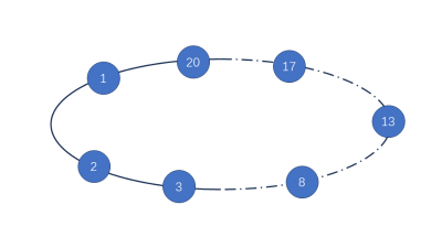
Figure 1:  Network topology of $20$ agents

Network: The experiments are conducted over a fixed undirected connected graph $\mathcal{G}$ which is shown in Fig. 1. The adjacency matrix $W$ is constructed as

$$W_{ij}=\left\{\begin{aligned} \frac{1}{{\rm deg}(i)+1}&,\ \text{if}\ i\neq j,(i,j)\in\mathcal{E},\\ 0\hskip 20.00003pt&,\ \text{if}\ i\neq j,(i,j)\notin\mathcal{E},\\ 1-\sum_{j\in\mathcal{N}_{i}}W_{ij}&,\ \text{if}\ i=j,\end{aligned}\right.$$

where $\mathrm{deg}(i)$ is the degree of agent $i$. For DPMM, we use $\text{\L}=(I-W)/2$, and simply set parameters $\theta_{i}\equiv\theta$, $\alpha_{i}\equiv\alpha$, $\gamma_{i}\equiv\gamma$ in their theoretical ranges presented in Proposition 2.

Subproblem: The following two examples are both constrained convex optimization problems with $\ell_{1}$-norm regularization. If we use DPMM and other alternative algorithms listed in Table 1 to solve them, the objectives of their subproblems have a unified form: $\psi_{i}(\mathrm{x}_{i})=s_{i}(\mathrm{x}_{i})+\lambda_{i}\|\mathrm{x}_{i}\|_{1}+\delta_{\Omega_{i}}(\mathrm{x}_{i})$, where $\delta_{\Omega_{i}}(\mathrm{x}_{i})$ is the indicator function on a box subset $\Omega_{i}$, and $s_{i}(\mathrm{x}_{i})$ is the smooth part of $\psi_{i}$. A fact is that both the proximal operators of the functions $\delta_{\Omega_{i}}(\cdot)$ and $\|\cdot\|_{1}$ have closed-form solutions. We then adopt the Davis-Yin splitting algorithm [37] to minimize $\psi_{i}(\mathrm{x}_{i})$. The subdifferential $\partial\psi_{i}(\mathrm{x}_{i})=\nabla s_{i}(x_{i})+\lambda_{i}\partial\|\mathrm{x}_{i}\|_{1}+\mathrm{N}_{\Omega_{i}}(\mathrm{x}_{i})$, where the sum $\lambda_{i}\partial\|\mathrm{x}_{i}\|_{1}+\mathrm{N}_{\Omega_{i}}(\mathrm{x}_{i})$ is a polyhedral set, precisely, $\lambda_{i}\partial\|\mathrm{x}_{i}\|_{1}+\mathrm{N}_{\Omega_{i}}(\mathrm{x}_{i})=[L_{i},U_{i}]$, the values of $L_{i}$ and $U_{i}$ depend on $\mathrm{x}_{i}$. At each iteration $k$, we use the following criterion (cf. (3.7)) as the stopping condition to calculate $\mathrm{x}_{i}^{k+1}$ such that $\mathrm{x}_{i}^{k+1}=\arg\min\psi_{i}^{k}(\mathrm{x}_{i})=s_{i}^{k}(\mathrm{x}_{i})+\lambda_{i}\|\mathrm{x}_{i}\|_{1}+\delta_{\Omega_{i}}(\mathrm{x}_{i})$,

$$\mathrm{dist}(0,\partial\psi_{i}^{k}(\mathrm{x}_{i}^{k+1}))=\left\|-\nabla s_{i}^{k}\left(\mathrm{x}_{i}^{k+1}\right)-\mathcal{P}_{[L_{i}^{k},U_{i}^{k}]}\left(-\nabla s_{i}^{k}(\mathrm{x}_{i}^{k+1})\right)\right\|_{\infty}\leq\varepsilon_{i}^{k}.$$

We set $\varepsilon_{i}^{k}\equiv 10^{-10}$ for the alternative algorithms in Table 1. The algorithm proposed in this paper is denoted by DPMM-$\varepsilon_{i}^{k}$ with some value of $\varepsilon_{i}^{k}$. The optimal value $F^{*}$ and the optimal solution $\mathrm{x}^{*}$ (if unique) of these two examples are calculated by the convex optimization toolbox CVX with the precision tuned to ‘best’.

5.1 Example 1

Considering the following example of (P) with $m=20$, $n_{i}=p=3$, $\forall\ i\in\mathcal{V}$, $q=0$,

$$\min_{\mathrm{x}}F(\mathrm{x})=\sum_{i=1}^{m}\bigg{(}\log\left(1+\exp\left(a_{i}^{\top}\mathrm{x}_{i}\right)\right)+\lambda_{i}\|\mathrm{x}_{i}\|_{1}\bigg{)}$$ (5.1)

$${\rm s.t.}\quad\sum_{i=1}^{m}A_{i}\mathrm{x}_{i}=0,\ l_{i}\leq\mathrm{x}_{i}\leq u_{i},\ \forall i\in\mathcal{V},$$

where data $a_{i},A_{i},l_{i},u_{i}$ are randomly generated, $\lambda_{i}=i/m^{2}$. This linearly constrained logistic regression problem with $\ell_{1}$-norm regularization is often encountered in machine learning.

We execute the DPMM-$\varepsilon_{i}^{k}$ with $\varepsilon_{i}^{k}=10^{-10}$, Tracking-ADMM [3], PDC-ADMM [6], and NECPD [4] for example (5.1) on a standard PC. All the algorithm parameters are fine-tuned in their theoretical ranges. We let all the algorithms start from the same initial decision vector.

In Fig. 2, we plot the objective residuals and the constraint violations generated by the aforementioned four algorithms during 1000 iterations. The objective residual is defined as $|F(\mathrm{x}^{k})-F^{*}|/|F^{*}|$. The constraint violation is $\|\sum_{i=1}^{m}A_{i}\mathrm{x}_{i}^{k}\|_{\infty}$.

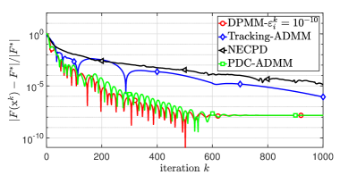
(a) Evolution of the objective residuals.

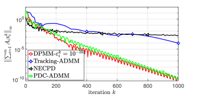
(b) Evolution of constraint violations.

Figure 2: Convergence performance of algorithms

In Fig. 2, the Tracking-ADMM and NECPD algorithms exhibit near convergence speed for solving Example (5.1). It is well-known that the quadratic proximal term $\frac{\gamma^{k}}{2}\|\mathrm{x}_{i}-\mathrm{x}_{i}^{k}\|^{2}_{2}$ of the objective of a subproblem brings significant benefits to the convergence of algorithms. However, the coefficient $\gamma^{k}$ of the NECPD algorithm tends to infinity at a rate of $O(k)$. As the algorithm runs, a large value of $\gamma^{k}$ may slow down its convergence speed. Tracking-ADMM incorporated the idea of gradient-tracking [12], where the connected graph with few edges may delay the consensus of the variable values it tracks, thereby leading to slow convergence. In contrast, over a low connectivity graph ($20$ nodes and $20$ edges), DPMM and PDC-ADMM demonstrate a fast convergence speed with respect to optimality and feasibility.

In communication costs, DPMM only requires one round of communication to exchange agents’ estimates $\mathrm{y}_{i}^{k}$ of the Lagrange multiplier at each iteration. Tracking-ADMM also communicates one round but exchanges two variable values. The number of communication rounds per iteration for PDC-ADMM and NECPD are $2$ and $d-1$, respectively, where $d$ is the degree of the minimal polynomial of the adjacency matrix $W$. Communication-wise, DPMM is more efficient than these three algorithms.

5.2 Example 2

Considering the following example of (P) with $m=20$, $n_{i}=p=3$, $q=1$,

$$\min_{\mathrm{x}}F(\mathrm{x})=\sum_{i=1}^{m}\bigg{(}\frac{1}{2}\|C_{i}\mathrm{x}_{i}-d_{i}\|_{2}^{2}+\lambda_{i}\|\mathrm{x}_{i}\|_{1}\bigg{)}$$ (5.2)

$${\rm s.t.}\quad\sum_{i=1}^{m}A_{i}\mathrm{x}_{i}=b,\ l_{i}\leq\mathrm{x}_{i}\leq u_{i},\forall\ i\in\mathcal{V}.$$

$$\hskip 22.0pt\sum_{i=1}^{m}\log\left(1+\exp\left(a_{i}^{\top}\mathrm{x}_{i}\right)\right)\leq f.$$

This constrained LASSO problem is also considered by [8]. Each matrix $C_{i}$ is symmetric positive definite and randomly generated. $b=\sum_{i=1}^{m}A_{i}\xi_{i}$ with $\xi_{i}$ being randomly chosen from a uniform distribution over the box $[l_{i},u_{i}]$. To ensure Assumption 3 be satisfied, we take $f>\sum_{i=1}^{m}\log\left(1+\exp\left(a_{i}^{\top}\xi_{i}\right)\right)$. $\lambda_{i}=i/m^{2}$, $A_{i},\ a_{i},$ and $d_{i}$ are randomly generated, $\forall\ i=1,2,\dots,m$.

We run the IPLUX algorithm [8] and DPMM-$\varepsilon_{i}^{k}$ with $\varepsilon_{i}^{k}=10^{-10},1/k^{2}$, and $1/k^{1.2}$ on a standard PC to solve example (5.2). Again, we choose the same initial decision vector $\mathrm{x}^{0}$ for both algorithms and then compare the practical convergence performance with their parameters tuned within respective theoretical ranges.

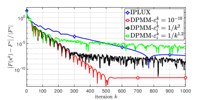
(a) Evolution of objective residual.

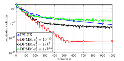
(b) Evolution of constraint violation.

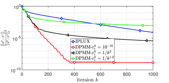
(c) Evolution of optimality error.

Figure 3: Convergence performance of algorithms

In Fig. 3, we plot the objective residual, constraint violation, and optimality error of running DPMM-$\varepsilon_{i}^{k}$ and IPLUX for 1000 iterations. The constraint violation is the sum of $\|\sum_{i=1}^{m}A_{i}\mathrm{x}_{i}^{k}-b\|_{\infty}$ and $\max\big{\{}\sum_{i=1}^{m}\log\left(1+\exp\left(a_{i}^{\top}\mathrm{x}_{i}\right)\right)-f,0\big{\}}$. The optimality error is $\|\mathrm{x}^{k}-\mathrm{x}^{*}\|_{2}/\|\mathrm{x}^{0}-\mathrm{x}^{*}\|_{2}$.

As illustrated in Fig. 3(a) and Fig. 3(b), the IPLUX algorithm effectively solves Example 2, reaching a theoretical convergence rate of $O(1/k)$ concerning the objective residuals and constraint violations, while Fig. 3(c) shows the slow progression of its decision variable sequence $\{\mathrm{x}_{k}\}$ towards the optimal solution $\mathrm{x}^{*}$. It can be summarized from Fig. 3 that the DPMM-$\varepsilon_{i}^{k}$ algorithm has a significant convergence speed advantage over IPLUX for solving the constrained LASSO problem (5.2), in terms of the optimal errors, objective residuals, and constraint violations.

Fig. 3 also indicates that the DPMM-$\varepsilon_{i}^{k}$ can be applied to a wider range of practical optimization problems, as we can see, with a dynamic precision $\varepsilon_{i}^{k}=1/k^{2}$ to compute the subproblem, running the DPMM-$\varepsilon_{i}^{k}$ for about 500 iterations yields a trial solution reaching an accuracy of $10^{-5}$, in terms of the objective residual, constraint violation, and optimality error. Of course, the faster the computational error $\varepsilon_{i}^{k}$ of the subproblem decays to 0, the faster the DPMM-$\varepsilon_{i}^{k}$ algorithm converges, which is also reflected in Fig. 3.

The algorithmic parameter $\tau=\alpha+\gamma\lambda^{2}$ of IPLUX is influenced by the objective and constraint functions of the solved optimization problem, i.e., $\alpha\geq L_{f}+L^{2}$ and $\lambda\geq\|A^{s}\|_{2}$, where $L_{f}$ is the gradient Lipschitz constant of the smooth part of the objective function, $L_{h}$ is the Lipschitz constant of the coupled inequality constraint function $\sum_{i=1}^{m}h_{i}(\mathrm{x}_{i})$, and $A^{s}$ is the matrix in the sparse coupled linear constraint considered by IPLUX (which is merged with the global coupled constraint $\sum_{i=1}^{m}A_{i}\mathrm{x}_{i}=b$ in this paper). This means that IPLUX requires some prior knowledge of the solved optimization problems, e.g., knowledge of these Lipschitz constants mentioned above, which may need all agents’ communication to achieve. However, this concern does not exist for DPMM, reviewing Proposition 2 and Remark 2, the parameter selections of DPMM can be done without any knowledge of the Lipschitz constants associated with the solved optimization problem and the network structure of the connected undirected graph, which implies that DPMM is robust.

Communication-wise, recall that agents exchange the Lagrange multiplier estimates $\widehat{\mathrm{y}}_{i}^{k}$ once per iteration in the DPMM algorithm, while IPLUX doubles such communication costs, which indicates that DPMM is more efficient.

6 Conclusion

In this paper, we have developed a distributed proximal method of multipliers, referred to as DPMM, to address coupled constrained convex optimization problems over a fixed undirected connected network. We demonstrate its primal-dual convergence and an $o(1/k)$ rate for the first-order optimality residual under general convexity. Furthermore, under the structural assumption, DPMM converges linearly. Numerical simulations reveal that the proposed DPMM algorithm is efficient for (P), comparing with some alternative distributed constrained optimisation algorithms.

References

- [1] Angelia Nedić, Alex Olshevsky, and Wei Shi. Improved convergence rates for distributed resource allocation. In 2018 IEEE Conference on Decision and Control (CDC), pages 172–177, 2018.
- [2] Huaqing Li, Qingguo Lü, Xiaofeng Liao, and Tingwen Huang. Accelerated convergence algorithm for distributed constrained optimization under time-varying general directed graphs. IEEE Transactions on Systems, Man, and Cybernetics: Systems, 50(7):2612–2622, 2020.
- [3] Alessandro Falsone, Ivano Notarnicola, Giuseppe Notarstefano, and Maria Prandini. Tracking-admm for distributed constraint-coupled optimization. Automatica, 117:108962, 2020.
- [4] Yanxu Su, Qingling Wang, and Changyin Sun. Distributed primal-dual method for convex optimization with coupled constraints. IEEE Transactions on Signal Processing, 70:523–535, 2022.
- [5] Yan Zhang and Michael M. Zavlanos. A consensus-based distributed augmented lagrangian method. In 2018 IEEE Conference on Decision and Control (CDC), pages 1763–1768, 2018.
- [6] Tsung-Hui Chang. A proximal dual consensus admm method for multi-agent constrained optimization. IEEE Transactions on Signal Processing, 64(14):3719–3734, 2016.
- [7] Andrea Camisa, Francesco Farina, Ivano Notarnicola, and Giuseppe Notarstefano. Distributed constraint-coupled optimization via primal decomposition over random time-varying graphs. Automatica, 131:109739, 2021.
- [8] Xuyang Wu, He Wang, and Jie Lu. Distributed optimization with coupling constraints. IEEE Transactions on Automatic Control, 68(3):1847–1854, 2023.
- [9] Alessandro Falsone, Kostas Margellos, Simone Garatti, and Maria Prandini. Dual decomposition for multi-agent distributed optimization with coupling constraints. Automatica, 84:149–158, 2017.
- [10] Shu Liang, Le Yi Wang, and George Yin. Distributed dual subgradient algorithms with iterate-averaging feedback for convex optimization with coupled constraints. IEEE Transactions on Cybernetics, 51(5):2529–2539, 2021.
- [11] Changxin Liu, Huiping Li, and Yang Shi. A unitary distributed subgradient method for multi-agent optimization with different coupling sources. Automatica, 114:108834, 2020.
- [12] A. Nedić, A. Olshevsky, and W. Shi. Achieving geometric convergence for distributed optimization over time-varying graphs. Siam Journal on Optimization, 27(4):2597–2633, 2017.
- [13] Shu Liang, Le Yi Wang, and George Yin. Distributed smooth convex optimization with coupled constraints. IEEE Transactions on Automatic Control, 65(1):347–353, 2020.
- [14] Alessandro Falsone and Maria Prandini. Augmented lagrangian tracking for distributed optimization with equality and inequality coupling constraints. Automatica, 157:111269, 2023.
- [15] B.S. He and X.M. Yuan. On construction of splitting contraction algorithms in a prediction-correction framework for separable convex optimization. arXiv e-prints, page arXiv:2204.11522, 2022.
- [16] Wei Shi, Qing Ling, Gang Wu, and Wotao Yin. A proximal gradient algorithm for decentralized composite optimization. IEEE Transactions on Signal Processing, 63(22):6013–6023, 2015.
- [17] Wei Shi, Qing Ling, Gang Wu, and Wotao Yin. Extra: An exact first-order algorithm for decentralized consensus optimization. SIAM Journal on Optimization, 25(2):944–966, 2015.
- [18] Lin Xiao and Stephen Boyd. Fast linear iterations for distributed averaging. Systems and Control Letters, 53(1):65–78, 2004.
- [19] Ali H. Sayed. Diffusion adaptation over networks. In Academic Press Library in Signal Processing, volume 3, pages 323–453. Elsevier, Boston, 2014.
- [20] Tamer Başar, Seyed Rasoul Etesami, and Alex Olshevsky. Convergence time of quantized metropolis consensus over time-varying networks. IEEE Transactions on Automatic Control, 61(12):4048–4054, 2016.
- [21] P. Combettes and H. Bauschke. Convex Analysis and Monotone Operator Theory in Hilbert Spaces. Springer International Publishing, New York, NY, 2017.
- [22] Etienne Corman and Xiaoming Yuan. A generalized proximal point algorithm and its convergence rate. SIAM Journal on Optimization, 24(4):1614–1638, 2014.
- [23] Jonathan Eckstein and Dimitri P. Bertsekas. On the douglas—rachford splitting method and the proximal point algorithm for maximal monotone operators. Mathematical Programming, 55:293–318, 1992.
- [24] Min Tao and Xiaoming Yuan. On the optimal linear convergence rate of a generalized proximal point algorithm. Journal of Scientific Computing, 74:826–850, 2018.
- [25] Feng Ma. Convergence study on the proximal alternating direction method with larger step size. Numerical Algorithms, 85:399–425, 2020.
- [26] Bingsheng He, Feng Ma, and Xiaoming Yuan. Optimal proximal augmented lagrangian method and its application to full jacobian splitting for multi-block separable convex minimization problems. IMA Journal of Numerical Analysis, 40(2):1188–1216, 2020.
- [27] Rockafellar R.T. Augmented lagrangians and applications of the proximal point algorithm in convex programming. Mathematics of Operations Research, 1(2):97–116, 1976.
- [28] Roger A. Horn and Fuzhen Zhang. Basic Properties of the Schur Complement. Springer US, Boston, MA, 2005.
- [29] R Tyrrell Rockafellar and Roger J-B Wets. Variational analysis. Springer-Verlag, Berlin, Heidelberg, 2004.
- [30] Jane J. Ye, Xiaoming Yuan, Shangzhi Zeng, and Jin Zhang. Variational analysis perspective on linear convergence of some first order methods for nonsmooth convex optimization problems. Set-Valued and Variational Analysis, 29:803–837, 2021.
- [31] Xiaoming Yuan, Shangzhi Zeng, and Jin Zhang. Discerning the linear convergence of admm for structured convex optimization through the lens of variational analysis. The Journal of Machine Learning Research, 21(83):1–75, 2020.
- [32] Zhi-Quan Luo and Paul Tseng. On the linear convergence of descent methods for convex essentially smooth minimization. SIAM Journal on Control and Optimization, 30(2):408–425, 1992.
- [33] Hui Zou and Trevor Hastie. Regularization and variable selection via the elastic net. Journal of the Royal Statistical Society Series B: Statistical Methodology, 67(2):301–320, 03 2005.
- [34] Robert Tibshirani, Michael Saunders, Saharon Rosset, Ji Zhu, and Keith Knight. Sparsity and smoothness via the fused lasso. Journal of the Royal Statistical Society Series B: Statistical Methodology, 67(1):91–108, 12 2004.
- [35] Howard D Bondell and Brian J Reich. Simultaneous regression shrinkage, variable selection, and supervised clustering of predictors with oscar. Biometrics, 64(1):115–123, 2008.
- [36] Stephen M. Robinson. Some continuity properties of polyhedral multifunctions. Mathematical Programming, 14:206–214, 1981.
- [37] D. Davis and W. T. Yin. A three-operator splitting scheme and its optimization applications. Set-Valued and Variational Analysis, 25:829–858, 2017.