Honeybee-like collective decision making in a kilobot swarm

Abstract

Drawing inspiration from honeybee swarms’ nest-site selection process, we assess the ability of a kilobot robot swarm to replicate this captivating example of collective decision-making. Honeybees locate the optimal site for their new nest by aggregating information about potential locations and exchanging it through their waggle-dance. The complexity and elegance of solving this problem relies on two key abilities of scout honeybees: self-discovery and imitation, symbolizing independence and interdependence, respectively. We employ a mathematical model to represent this nest-site selection problem and program our kilobots to follow its rules. Our experiments demonstrate that the kilobot swarm can collectively reach consensus decisions in a decentralized manner, akin to honeybees. However, the strength of this consensus depends not only on the interplay between independence and interdependence but also on critical factors such as swarm density and the motion of kilobots. These factors enable the formation of a percolated communication network, through which each robot can receive information beyond its immediate vicinity. By shedding light on this crucial layer of complexity –the crowding and mobility conditions during the decision-making–, we emphasize the significance of factors typically overlooked but essential to living systems and life itself.

I Introduction

Collective decision-making is the process by which a group of agents makes a choice that cannot be directly attributed to any individual agent but rather to the collective as a whole [1]. This phenomenon is observed in both natural and artificial systems, and it is studied across various disciplines, including sociology, biology, and physics [2, 3]. In particular, social insects have long been recognized for their fascinating behaviors, and collective decision-making is no exception. An intriguing example of this can be found in the way honeybees choose their nest sites [4, 5, 6, 7]. This specific problem has been the focus of numerous models of collective decision-making in honeybees [8, 9, 10, 11, 12] and serves as an inspiration for our study.

The process of collective decision-making can encompass a virtually infinite number of choices. For instance, in flocking dynamics, individuals often have to converge on a common direction of motion [13, 14, 15, 16, 17]. In such cases, achieving consensus in favor of an option is the result of a continuous process. Another category of collective decision-making involves a finite and countable set of choices. Typical models in this category require a group of individuals to collectively determine the best option out of a set of $n$ available choices [18]. Here, the consensus-reaching process becomes a discrete problem. In real-life scenarios, examples of such decision-making processes include selecting foraging patches, travel routes or candidates in a democratic election. Within this countable set of choices, consensus is achieved when a large majority of individuals in the group favor the same option. The threshold for what constitutes a ‘large majority’ is typically defined by the experimenter but generally signifies a cohesive collective decision with more than 50% agreement among the individuals [18]. In these collective decision-making models, each option is characterized by attributes that determine its relative desirability. For instance, in the context of selecting a potential nesting site for honeybees, these attributes could include size, distance, and vegetation type. Measures of quality and cost for each potential option encompass these attributes [19]. These two properties can be configured in multiple ways. The simplest scenario occurs when options’ qualities and costs are the same for all available options, referred to as symmetric. In such a scenario, the group faces the challenge of breaking symmetry when selecting an option, often resulting from the amplification of random fluctuations [19]. In all other scenarios, the decision-making process is influenced by the specific combination of qualities and costs among different options. For example, in cases where the cost varies among options, making it asymmetric, but the qualities are symmetric, the option with the minimum cost is typically considered the best choice [20]. Conversely, in situations with asymmetric qualities but symmetric costs, the option with the maximum quality tends to be chosen [21].

Opinion dynamics models are proposed and developed to examine how individuals communicate and make decisions within groups. These models consist of a group of agents, each with their own instantaneous opinion or ‘state’. Individuals interact with one another and revise their opinions based on the opinions of others. Among the simplest models used to study collective decision-making are the well-known voter model [22, 23] or the majority rule model [24]. These models are limited in that they assume that all agents are equally likely to adopt either opinion. In reality, however, individuals may have different preferences, beliefs, or biases that can influence their decision-making. To address this limitation, more complex models have been developed that incorporate features such as stubbornness, partisanship, and heterogeneity [25, 26]. These models generally help to understand how opinion diversity and polarization can arise in groups, and how these dynamics might be influenced by different factors.

In this work, our primary focus will be to determine whether a swarm of autonomous mini-robots, in particular kilobots, can achieve high levels of consensus for the best quality option, in a general scenario where robots both move and engage in opinion spreading strategies simultaneously in a decentralized manner. This introduces a level of complexity beyond that of a model on a lattice or a network. Aside from the general insights we can gain from studying opinion dynamics with moving individuals, this scenario possesses the distinctive feature of being closer to the behavior observed in the social animal world, where a diversity of intriguing signalling mechanisms have been previously identified [27]. In particular, crowding and clustering effects stand out as highly relevant from our study. As they were shown to be crucial for honeybees in trophallaxis [28], they might also be decisive in communication and collective decision making.

In the following, we motivate our work inspired by the honeybees’ house hunting problem in Sec. II, where we also present the particular discrete opinion-dynamics model under scrutiny. In Sec. III, we introduce our experimental study system, a kilobots swarm, and their emulator, Kilombo. Sections IV and V present our main results, which combine experiments on kilobots, numerical results on the Kilombo emulator, numerical simulations of the model on specific geometries, and their comparison to analytical results of the opinion-dynamics problem. Finally, in Sec. VI, we provide a discussion of our results and perspectives. Technical details about the model and the experimental setup are provided in Appendix A, and additional complementary analysis and data are included in Appendices B and C.

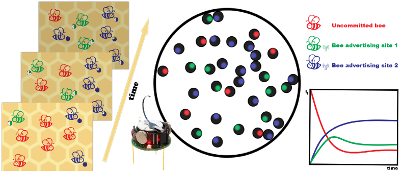
Figure 1: Schematics of the collective decision dynamics under scrutiny. The left column represents the dynamics of the decision model: at a given instant of time committed bees are advertising their state to convince undecided bees to commit to their option. The time they spend advertising their option will be directly related to the quality they perceive for that option. As time advances a build up for the better option is expected since it is benefited from longer advertisement periods. The central column shows a schematic representation of our kilobot experiments. Each kilobot has a LED that indicates its state, either uncommitted or committed to (and advertising for) site 1 or 2. The right column displays schematically how the different proportions of bees on each state evolve in time, starting from a totally uncommitted population.

II Modeling the nest site selection problem in honeybees

Honeybees are social insects that reside in large colonies. The way scout honeybees select new nest sites represents an interesting example of a collective decision-making process that involves a combination of individual and group behaviors. In recent years, researchers have made significant progress in understanding the mechanisms behind this behavior, which is crucial for the survival and reproduction of honeybee colonies [29, 30, 7].

The process of collective decision-making in honeybees has primarily been studied in the species Apis mellifera. Towards the end of spring, honeybee colonies split, with approximately two-thirds of the colony leaving the nest along with the queen in search of a new nesting site. During this process, a fraction of the swarm scouts the surroundings to gather information about potential new sites, assessing their quality based on traits such as size, food availability, or the degree of concealment [5, 29]. When a scout bee discovers a promising new nesting site, it returns to the swarm and communicates information about the site fitness and location to other bees through the intricate waggle dance [31, 32]. Doing so, she may recruit other scout bees that remained in the swarm to also explore - and subsequently advertise - the same location. The duration of the waggle dance is correlated with the honeybee’s perception of the site’s quality. A longer and more animated dance indicates a more suitable nest site, while a shorter and less dynamic dance corresponds to a less desirable site [33]. Consequently, high-quality sites receive longer and more frequent advertising, while low-quality sites see reduced attention, resulting in an overall increase in the number of bees visiting and dancing for high-quality sites and a decrease in those doing so for low-quality ones.

In addition to their quality, each site also has its associated cost, which represents the likelihood that a scout bee will discover the site, considering factors such as distance or concealment. This leads to the possibility that some high-quality options may go unnoticed due to their associated costs. Over time, the dances performed by the honeybees tend to converge on a single site, and once a potential nest site has attracted a sufficient number of bees, a quorum is formed, ideally in favor of the best available option. This entire process ensures that the migrating part of the colony moves together to their new home [30].

Model of a fully-connected scout bee network

Several mathematical models of the honeybee nest-site selection problem have been proposed in the literature [8, 34, 9, 35, 10, 36]. In particular, List, Elsholtz, and Seeley [10] introduced an agent-based model inspired by the decision-making process of honeybees. This model integrates both an individual’s self-discovery of potential nest sites and the existing interdependencies, which encompass interactions among bees, leading to imitation and the adoption of sites presented by other bees. The model explicitly incorporates various parameters, including the number of sites, site quality, site self-discovery probabilities, and group interdependence. Here, we adopt a very similar approach to describe the rules that govern the behavior of our kilobot robots.

The nest-site choice model proposed in [10] consists of a swarm of $N$ scout bees that reach consensus and collectively decide on one of the potential nest sites, labeled $1,2,3,...,k$. Each site $j$ has an intrinsic quality $q_{j}\geq 0$ that determines the time a bee spends advertising site $j$ through the waggle dance. At time $t$, a bee can either be dancing for one of the $k$ sites (i.e., promoting it) or not dancing for any site, indicating that it is still searching for a site, observing other bees’ dances, or simply resting. Formally, a vector $x_{i,t}=(s_{i,t},d_{i,t})$ represents the state of bee $i$ at time $t$, where $s_{i,t}=0$ if bee $i$ is not dancing for any site. When a bee is dancing, $s_{i,t}=1,\ldots,k$, indicating the site the bee is promoting, and $d_{i,t}$ represents the remaining duration of bee $i$’s waggle dance. In each discrete time-step (which sets the unit of time in the model), the states of bees are updated in parallel. While a bee is dancing for a site, its dance duration $d_{i,t}$ decreases by one time unit in each time-step until it reaches zero, at which point the bee stops advertising, and its state returns to the non-dancing value $s_{i,t}=0$. Non-dancing bees have a probability $p_{i,t+1}$ of starting to dance for site $j$ at time $t+1$. When this occurs, $s_{i,t+1}=j$, and the duration of the new dance is set equal to or proportional to the site quality. Here we use $d_{j,t+1}=q_{j}$. There is also a probability of remaining uncommitted to any site, $p_{0,t+1}$. A normalization condition is imposed such that $\sum_{j=0}^{k}p_{j,t+1}=1$. The probability $p_{j,t+1}$ estimates the likelihood of a bee finding site $j$ and committing to advertising it. It is calculated as follows:

$$p_{j,t+1}=(1-\lambda)\pi_{j}+\lambda f_{j,t}.$$ (1)

Here, $\pi_{j}$ represents the a priori self-discovery probability of site $j$, i.e, the likelihood that a scout bee finds site $j$ independently of other bees. $\lambda$ denotes the bees’ interdependence, and $f_{j,t}$ represents the proportion of bees already dancing for site $j$ at time $t$. It is important to note that we also have the normalization condition $\sum_{j=0}^{k}f_{j,t}=1$. The interdependence parameter $\lambda$ ranges between $0$ and $1$, determining the extent to which bees rely on each other to decide to dance for a site. When $\lambda=0$, the probability of finding site $j$ depends solely on the self-discovery probability $\pi_{j}$, regardless of the proportion of bees dancing for it. Conversely, as $\lambda$ approaches $1$, the probability of committing to site $j$ at time $t+1$ becomes almost entirely dependent on the proportion of bees already dancing for it at time $t$, denoted as $f_{j,t}$. In other words, a higher value of $\lambda$ means that committing probability relies more on imitation of other bees. The self-discovery probabilities of available sites $\pi_{j}$ are chosen in a way that ensures $\sum_{j=1}^{k}\pi_{j}<1$, and in general, the sum does not exceed the maximum value of approximately 0.6, which corresponds to a 60% probability of independent commitment to any available nest site.

It’s worth emphasizing that in this model, every bee can observe the dancing state of all other bees in the swarm, regardless of their relative separation. In this regard, the model developed by List et al. represents a mean-field stochastic agent-based model. Galla [36] formulated a master equation for the commitment probabilities within the same model as presented in [10]. In this formulation, he replaces the fixed duration $d_{j}=q_{j}$ of the waggle dances with stop-dancing rates $r_{j}=1/q_{j}$. Following this approach, it is possible to derive non-linear differential equations that describe the evolution of the average values $\langle f_{j,t}\rangle$. These equations closely align with the results obtained from the original stochastic model. Furthermore, in the long time limit, one can analytically determine the stationary values of $\langle f_{j,t}\rangle$ using this mean-field approximation. Appendix A.1 provides a brief description of this approach. Our model simulations implement the same stochastic method.

Model of quenched bee configurations

Our analysis will also consider the limiting case of random static, and generally non fully-connected, configurations of agents, the quenched configuration limit, on which we run the same collective bee-like decision model. In this limit, the global proportions $f_{j,t}$ of agents in $j$ state appearing in Eq. 1, as considered in the original model of List et al. [10], are replaced by local proportions of agents computed from a fixed list of ‘neighbors’ for each individual $i$ in the group. Lists of neighbors are computed after introducing a finite communication radius $r_{\tt int}$ around each agent in a random quenched configuration to identify other agents in this circular area of influence. These lists are calculated only once for each random configuration, and remain unchanged during the decision dynamics.

III Experimental kilobot swarm

In this study, we use a kilobot swarm as our experimental system for investigating consensus reaching and exploring the interplay between the two most important factors in the honeybee-like nest-site selection model proposed by List et al., i.e. independent discovery and imitation.

Kilobots are compact open-source swarm robots, measuring 3.3 cm in diameter and 3.4 cm in height, purpose-built for the study of collective behavior [37]. Our primary goal is to experimentally investigate how the introduction of restricted robot communication capabilities (or local interactions), robot locomotion and spatial constraints, impact consensus reaching in comparison to the bee-like models introduced in Sec. II. These mini-robots have previously been used to study collective decision-making [38], pattern formation [39], morphogenesis [40], space exploration [41], collective transport of objects [42] in different experimental setups, and morphological computation and decentralized learning [43].

Kilobots’ locomotion, decentralized control and information exchange

Kilobots feature three slender, metallic legs—one in the front and two at the back. With calibrated lateral vibrating motors, they can effectively overcome static friction, enabling self-propulsion. Moreover, they have the capability to rotate either clockwise or counter-clockwise by selectively activating one of the two vibrating motors. Kilobots are equipped with an Arduino controller, memory storage, and an infrared transmitter and receiver for bidirectional communication. Within an interaction radius of up to $10$ cm, kilobots can exchange messages with nearby robots, with each message carrying up to $9$ bytes of information. During communication, the receiving robot assesses the intensity of incoming infrared light, enabling it to calculate relative distances to neighboring robots.

Each kilobot in the swarm can execute various user-programmed instructions and functions, with each processing cycle (or loop iteration) representing a unit of time in their dynamics. During our experiments, kilobots exist in discrete states, and their current state is visually conveyed through RGB LED lights. This makes kilobots an ideal experimental system for studying collective decision-making, combining decentralized activity, limited communication capabilities and locomotion —effectively making them ‘programmable insects’.

We place up to $35$ kilobots in a circular arena with a radius $R$ delimited by rigid walls. Using an azimuthal camera, we capture the kilobot activity in accordance with the guidelines of the nest-site selection model outlined in the previous section (see also Fig. 1). Further details about the robots technical features and about the experimental setup are presented in Appendix A.2.

Kilombo: the kilobot swarm emulator

A useful tool to work alongside physical experiments is the kilobot-specific simulator software Kilombo[44]. This is a C-based simulator that allows the code developed for simulations to be run also on the physical robots, removing the slow and error prone step of converting code to a different platform. In this way we can also perform simulations using Kilombo, to test our experimental setup and to support our results - and to complement them whenever it has not been possible to perform further experiments.

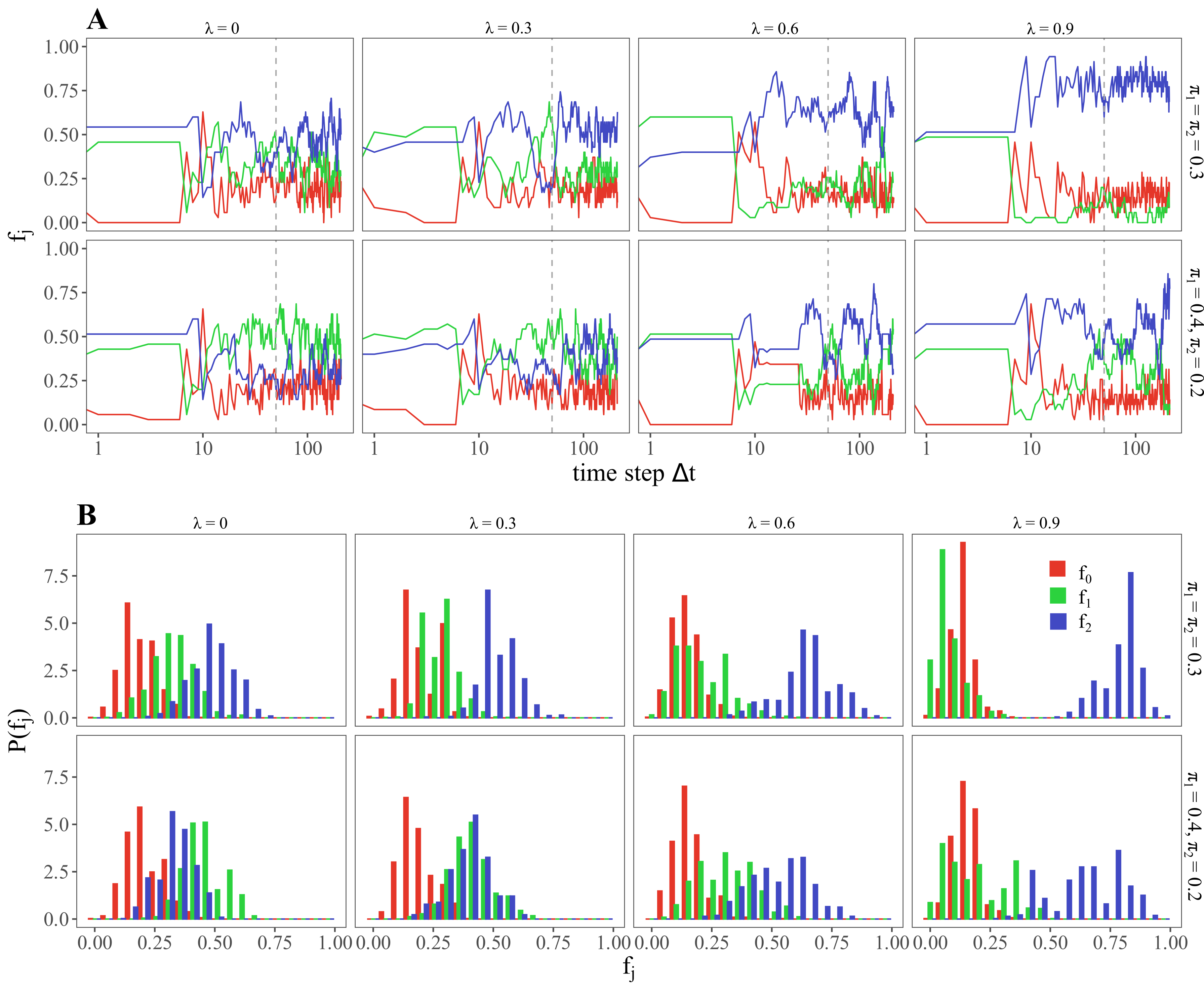
Figure 2: A: Proportions of kilobots $f_{j}$ dancing for the different states as a function of time. Red, green and blue represent the proportion of uncommitted ($f_{0}$) and dancers for low-quality ($f_{1}$) and high-quality ($f_{2}$) sites, respectively. B: Histograms of $f_{j}$ values in the stationary state. Plots correspond to symmetric (up) an asymmetric (bottom) a priori discovery probabilities, and to interdependence parameter values $\lambda={0,0.3,0.6,0.9}$ (left to right). Five repetitions of the experiment for each $\lambda$ were performed, both for the symmetric discovery with $\pi_{1}=\pi_{2}=0.30$ and for the asymmetric discovery with $\pi_{1}=0.40,\pi_{2}=0.20$.

IV Consensus reaching in a bee-like kilobot swarm

In this section we describe, both experimentally and theoretically, how the complex decision-making problem of reaching strong consensus for the best-available option is solved by our bee-like kilobot ensemble under different conditions. Essentially, we analyze the temporal dynamics of the proportion of bees (bots) that either advocate for one of the possible sites or remain uncommitted. We examine how these proportions evolve and eventually stabilize, while also exploring the criteria that signify the attainment of a consensus in this steady state. We compare our experimental results and Kilombo simulations with mean-field theoretical results finding intriguing resemblances in sufficiently crowded conditions, or after long enough exploration times, but also hints towards important divergences in other plausible conditions. By implementing the nest-site selection model within a physical kilobot system, we gain the capacity to explore the consequences of more realistic robot interactions and the role of space and locality on consensus formation.

Collective decision-making in kilobots

We start by running our experiments in a group of $N=35$ kilobots. We deploy the kilobots within a circular arena of radius $R=20$ cm and task them with assuming the role of scout bees. These kilobots engage in a dynamic process defined by the List et al. model, as elaborated in Sec. II. Each kilobot holds an internal state and displays it with a color LED. Throughout the course of the experiment, kilobots adjust their internal states based on the probabilities outlined in Eq. 1, but having only partial and individual information of the population of bees advertising each site, $f_{i,t}$. The computation of these values takes place after a given time-step, $\Delta t$, of the decision process relying on the information that each uncommitted kilobot can gather from its immediate surroundings.

While the typical outcomes of the List et al. model dynamics have been documented in prior research [10, 36], previous investigations have primarily scrutinized these developments either at the mean-field (fully-connected) level [10, 36] or within the context of nearest neighbor interactions within a square lattice [36]. In contrast, the present approach involves committed kilobots that move in the circular arena as persistent random walkers during their engagement in the advertising, or dancing, phase of the consensus-searching dynamics. This advertising movement results in a varying number of neighbors that they can communicate with . In order to correctly quantify the relevance of these factors, we first benchmark the communication capabilities of individual bots, as reported in App. B.

We narrow the focus of our experiments to the case of two sites: a high-quality site (designated as site $2$) and a lower-quality site (referred to as site $1$) . At each time-step kilobots are either dancing for site $1$, site $2$, or not advertising any site. As an extra feature towards emulating the natural behavior of honeybees, we introduce an explicit difference in the dynamics of committed and uncommitted kilobots. While kilobots advertising an option perform a persistent random walk (PRW), uncommitted kilobots, instead, come to a halt to wacth other kilobot advertisements.

We study both the time evolution and the steady state of the decision-making experiment on our bee-like kilobot system. The proportion of kilobots not advertising a site and the proportions of kilobots dancing for sites $1$ and $2$, also referred to as the dance frequencies $f_{0}$, $f_{1}$ and $f_{2}$, respectively, are monitored as a function of time until they stabilize and fluctuate around mean values. The duration required for the system to attain this steady state varies depending on the model’s parameters. Generally, large interdependence $\lambda$ leads to stronger majorities, while dragging out the evolution up to that state. Moreover, when the competing sites have similar qualities the swarm takes longer to reach a consensus. In our experiment, site qualities are fixed to $q_{1}=7$ and $q_{2}=10$; and thus, advertising times for site $1$ and $2$ are equal to $q_{1}\Delta t$ and $q_{2}\Delta t$, respectively .

In addition, our analysis encompasses the evolution under different levels of interdependence $\lambda$ and considers two distinct scenarios for the discovery probabilities $\pi$: a symmetric case where $\pi_{1}=\pi_{2}$ and an asymmetric case where $\pi_{1}>\pi_{2}$, favoring the lower-quality site.

Figure 2A illustrates the dynamics of $f_{0}$, $f_{1}$, and $f_{2}$ over time, for different $\lambda$ and for both the symmetric and asymmetric cases. The initial conditions are set as follows: $f_{1}(t=0)=f_{2}(t=0)\simeq 0.43$, and $f_{0}(t=0)\simeq 0.14$ (i.e. approximately $15$ kilobots dancing for site 1, $15$ dancing for site 2 and $5$ uncommitted). Other initial conditions have also been tested but, as expected, stationary results do not depend on the particular choice used in the experiments. The time evolution of each population is jerky and fluctuating. This behavior is also expected and is an inherent consequence of the model dynamics, as kilobots promoting a site revert to an uncommitted state after their dancing period concludes. Additionally, due to the limited system size, these fluctuations are particularly noticeable. Nevertheless, systematic behaviors can be grasped when examining mean values and full distributions. Across all values of $\lambda$, there exists a transient phase in which the larger population oscillates between the three states $j$, resulting in significant variations in the values of $f_{j}$. However, roughly after $\sim 50$ time-steps, a steady state is achieved, and each $f_{j}$ fluctuates around its mean value. In the scenario with symmetric $\pi$ values, irrespective of $\lambda$, $f_{2}$ eventually becomes the dominant population in the steady state. Moreover, increasing the interdependence parameter $\lambda$ amplifies the difference between the proportion of kilobots dancing for the high-quality site ($f_{2}$) and the low-quality site ($f_{1}$). Interestingly, when we shift towards asymmetric self-discovery probabilities ($\pi_{1}>\pi_{2}$), it is observed that if $\lambda$ is not sufficiently large, the steady state can be dominated by $f_{1}$ or present a stalemate between $f_{1}$ and $f_{2}$. However, increasing $\lambda$, the system gains the capability to favor the less accessible yet higher-quality option $2$.

Across all scenarios and parameter sets, there is notable dispersion in the values of $f_{j}$, resulting in broad probability distributions $P(f_{j})$ for all three $j$, as exhibited in Fig. 2B. When $\lambda$ is low, the distributions $P(f_{j})$ for all three states tend to overlap. However, with an increase in $\lambda$, the distributions $P(f_{1})$ and $P(f_{2})$ gradually separate from each other, eventually exhibiting significantly distinct mean values when the interdependence is at its highest, $\lambda=0.9$.

Consensus in numerical and analytical approaches

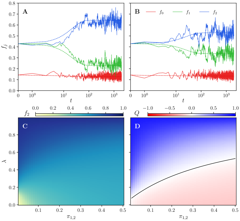
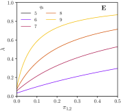
Figure 3: A-B: Dance frequencies $f_{0}$ (red), $f_{1}$ (green) and $f_{2}$ (blue) as a function of time obtained from numerical simulations of the stochastic model, and from the numerical integration of the mean-field deterministic equations (smooth superimposed curves in the same color). A: Symmetric discovery scenario with probabilities $\pi_{1}=\pi_{2}=0.3$. B: Asymmetric discovery scenario with probabilities $\pi_{1}=0.4$ and $\pi_{2}=0.2$. Other parameters are: $N=100$, $q_{1}=7$, $q_{2}=10$, and $\lambda=0.6$. Simulations were averaged over $100$ realizations. C-D: Stationary values of $f_{2}$ (C) and $Q$ (D) in the parameter space $(\pi_{1,2},\lambda)$ obtained from solutions of the deterministic equations of the model. The black line on (D) corresponds to the theoretical crossover line where $Q=0$. Parameters are $q_{1}=7$, and $q_{2}=10$. E: Consensus crossover lines or $\lambda$-thresholds for consensus, $\lambda^{*}$, i.e. $Q(\lambda^{*})=0$ as a function of $\pi_{1,2}$ (in the symmetric scenario, $\pi_{1}=\pi_{2}$). Colors represent different values of the low-quality site $q_{1}$, while $q_{2}=10$ is maintained constant.

In the following paragraphs we proceed with the numerical analysis of the nest-site selection problem within a fully connected system. Figure 3A-B presents the values of the dance frequencies $f_{0}$, $f_{1}$ and $f_{2}$ as a function of time. These values are obtained from both stochastic simulations and the numerical integration of the deterministic mean-field equations, as detailed in App. A.1. The observed curves are qualitatively similar to the ones displayed by the evolution of the model in kilobots (as shown in Fig. 2). It is worth noting that, as for the kilobots, we use $q_{1}=7$ and $q_{2}=10$. In both studied cases, whether symmetric ($\pi_{1}=\pi_{2}=0.30$) or asymmetric ($\pi_{1}=0.4$, $\pi_{2}=0.2$), with the same value of $\lambda=0.6$, we observe the high-quality nest site taking the lead in the steady state.

Simulations of the stochastic model display finite-size fluctuations around the mean values, whereas the numerical integration of the analytical solution produces smooth evolution curves. Notice that the analytical curves do not accurately represent the transient state at very short times, but they accurately describe the average stationary value for each parameter set. This reassuring result allows us to perform a parametric exploration of the model without the need of resource-intensive simulations.

Employing the analytical solution, we delve into the exploration of the parameter space defined by $\pi_{j}$ and $\lambda$. We do not only asses the stationary dance frequencies, $f_{j}$, but also a strong majority definition of consensus:

$$Q=f_{2}-2f_{1}\text{.}$$ (2)

This definition implies that there must be twice as many bees dancing for the high quality site than for the low quality site for the condition $Q>0$ to be met. Consequently, this represents a large majority consensus, i.e., a majority by a factor of $2/3$ in the case there were no uncommitted bees in the system.

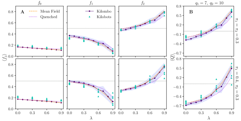
Figure 4: Stationary dance frequencies and consensus as a function of interdependence A: Average frequencies $\langle f_{0}\rangle$, $\langle f_{1}\rangle$ and $\langle f_{2}\rangle$ and B: Average consensus $\langle Q\rangle$ as a function of $\lambda$ for symmetric (up) and asymmetric (bottom) $\pi_{j}$ for physical kilobots, and for simulations using Kilombo, quenched configurations and fully-connected networks. Triangles: Mean values from experiments of $N=35$ kilobots (5 repetitions per parameter combination). Solid purple line with points: Mean values from Kilombo simulations with $N=35$ bots averaged over $50$ repetitions. Shaded area: Kilombo standard deviation. Dashed orange line: Mean values from simulations of the fully connected model with $N=35$ bots averaged over $100$ repetitions. Dotted pink line: Mean values from quenched configurations with $N=35$ bots averaged over $100$ repetitions.

In Fig. 3 (C-D) we present the outcome of the decision process in the symmetric scenario, $\pi_{1}=\pi_{2}$. We asses both the stationary value of $f_{2}$ (Fig. 3C) and the consensus, $Q$ (Fig. 3D). The exploration of the parameter space is done by varying the values of the interdependence $\lambda$ (y-axis) for each value of the self-discovery probabilities $\pi_{1,2}$ (x-axis) (a similar parameter space exploration for the asymmetric scenario is presented in the Supplementary Material [47]). The color charts illustrate how these two metrics vary across the parameter space. We observe a smoothly varying trend indicating that the proportion of individuals dancing for the high quality site $f_{2}$ increases along with the interdependence parameter $\lambda$, regardless of the specific value of $\pi_{1}$ and $\pi_{2}$. This phenomenon arises from bees placing more reliance on the opinions of their peers, and as $\lambda$ increases, it enhances the reinforcement for the best possible option. Contrarily, when both independent discoveries ($\pi_{1}=\pi_{2}$) increase simultaneously, there is a relative decrease in the number of bees dancing for site $2$. This means that as $\pi$ values increase while keeping $\lambda$ constant, more advertisements are motivated by independent discoveries rather than by opinion sharing. Consequently, when $\pi_{1}=\pi_{2}$, $f_{1}$, the population of bees dancing for site $1$ increases at the expense of site $2$, hindering overall consensus. In the extreme case of $\pi_{1}=\pi_{2}=0.5$, this translates in consensus never being achieved (i.e. $Q<0$) if the interdependence parameter is lower than $\sim 0.5$. The black line depicted in Fig. 3D corresponds to the strong consensus crossover $Q=0$, computed using the analytical solution. A system with a set of parameters given by points below this line will never find strong consensus, but it will do for a set of parameters given by a point above. In other words, after surpassing a $\pi_{1,2}$-dependent $\lambda$ threshold, $\lambda^{*}$, the system crosses over to a strong consensus state, $Q>0$, and the strength of this consensus intensifies with increasing interdependence. The region of non-consensus expands as $\pi_{1,2}$ values grow, thereby narrowing the range of interdependence values that lead to consensus.

Certainly, the ‘critical’ line $\lambda^{*}(\pi_{1},\pi_{2})$ is contingent upon the values of qualities $q_{1}$ and $q_{2}$ as well. In Fig. 3E, we represent $\lambda^{*}$ as a function of $\pi_{1}=\pi_{2}$, maintaining a fixed value of $q_{2}=10$ while exploring different choices of $q_{1}$. We observe that when $q_{1}$ is markedly smaller than $q_{2}$, particularly when $q_{1}\leq q_{2}/2$, the region of no strong consensus basically disappears, i.e., the swarm is able to choose the high quality site with strong majority, allowing for consensus even when $\lambda=0$. On the other hand, when $q_{1}$ increases and approaches the value of $q_{2}$, the competition between sites intensifies. Consequently, a higher value of $\lambda$ becomes necessary to counteract the influence of the discovery probabilities. As a mater of fact, it is worth emphasizing that the $\lambda^{*}$ curves do not depend on both the individual site qualities, but rather on their relative difference, denoted as $\Delta_{q}=(q_{2}-q_{1})/(q_{2}+q_{1})$ [48]. This relative difference plays a pivotal role in determining the critical threshold for consensus.

Comparison between experiments and simulations

We would like to quantitatively compare the steady-state averages in kilobots with those obtained from the modeling approaches. Our goal is to distinguish the emerging properties of the real system, which involves restricted communication capabilities, and moving individuals, in comparison to the fully-connected approximations made in mean-field solutions. To enhance this comparison, we utilize Kilombo [44], the kilobot’s emulator, to conduct complementary simulations under the same experimental conditions. On the other hand, alongside the fully-connected stochastic model simulations, we also incorporate the steady-state results obtained from simulations with quenched configurations of bots running the same collective decision-making model.

Figure 4 displays the average stationary values of the dance frequencies $\langle f_{0}\rangle$, $\langle f_{1}\rangle$, $\langle f_{2}\rangle$, and the consensus $\langle Q\rangle$ as functions of the interdependence parameter $\lambda$ for both symmetric and asymmetric scenarios defined by the same self-discovery probabilities $\pi_{i}$, and site-quality values $q_{1}=7$ and $q_{2}=10$, considered previously. Consistently, the primary trend is similar across all approaches: at small values of interdependence $\lambda$, the majority of the population gravitates towards the high-quality site ($2$) in the symmetric case. Conversely, it aligns with the low-quality site ($1$) when asymmetric self-discovery probabilities favor it. In this case, there is no consensus for the higher quality option, and $Q$ assumes negative values. As $\lambda$ increases, $\langle f_{1}\rangle$ decreases while $\langle f_{2}\rangle$ increases for both the symmetric and asymmetric scenarios. Moreover, $\langle f_{1}\rangle$ and $\langle f_{2}\rangle$ exhibit similar functional trends but in opposite directions, resulting in the stationary value of $\langle f_{0}\rangle$ remaining nearly independent of $\lambda$. When examining the stationary average of the strong consensus parameter $\langle Q\rangle$, we observe a smooth transition from non-consensus to consensus as $\lambda$ varies. This is rather a crossover more than a phase transition, but it can be precisely identified. Notably, in scenarios with symmetric discovery probabilities, consensus is achieved at smaller $\lambda$ values compared to asymmetric scenarios. This is because there is less introduction of independent discoveries for the low-quality site, leading to less misleading information that needs to be discarded through communication.

Now, let’s delve into a quantitative comparison of the different approaches, going beyond the observed consistency in the data. First, it’s noteworthy that the stationary values obtained from physical kilobots closely match those from Kilombo simulations, even within the standard error (represented by shaded areas). This alignment underscores the reliability of the emulator in complementing real measurements. More remarkably, both experimental and emulator results closely align with the mean-field results. This coincidence might be less expected, and we will discuss the reasons behind it for the chosen set of parameters. These findings suggest that mobile kilobots, as they interact with their local environment, can effectively sample the system’s state and transmit information throughout, almost as if they were fully connected, achieving collective decision-making comparable to mean-field fully-connected individuals. We will test this hypothesis in the next section. However, it’s worth noting that this agreement is not perfect. While $\langle f_{j}\rangle$ and $\langle Q\rangle$ values are nearly identical for all approaches at low values of $\lambda$, some differences become noticeable after an interdependence value of approximately $\lambda\sim 0.5$. In this range, quenched configurations exhibit higher $\langle f_{1}\rangle$ and lower $\langle f_{2}\rangle$ values than the fully-connected system. Furthermore, for high $\lambda$ values the experimental data also deviate from mean-field results . As a consequence of these variations, we observe a lower consensus value compared to the fully-connected case. Indeed, within a specific range of $\lambda$ values in the asymmetric discovery scenario, we even observe a lack of strong consensus in both quenched bots simulations and in several realizations of our bee-like kilobot experiments when compared to the fully-connected case.

In summary, in a high enough interdependent system, the experimental results displayed in Fig. 4 demonstrate that mobile individuals, such as kilobots moving in space and integrating information over time, are capable of achieving high consensus values comparable to fully-connected systems. The exact threshold depends on model parameters such as quality differences and self-discovery probabilities. Quenched configurations, characterized by fixed neighbor lists for interactions, help us assess the importance of kilobots’ movement and mixing under experimental conditions. Despite the limited communication range of kilobots, our hypothesis is that their mobility enables information to spread in a manner that the outcome of the decision-making problem becomes similar to mean-field results. However, in quenched configurations conditions, local consensus for the low-quality option may emerge, diminishing the chances of attaining strong consensus for the best-quality option. Low interdependence diminishes the impact of communication in individual decision-making, while increasing interdependence amplifies the relevance of communication for consensus.

V Information spreading in the kilobot swarm

In this section we provide a more detailed analysis of the information spreading taking place in our kilobot swarm as they play the bee-like decision-making process. Our aim is to investigate under which circumstances consensus reaching in physical kilobots can be almost as effective as in an idealized mean-field-like communicating system.

When analyzing the data presented in Figure 4, and observing the consistency between the fully-connected approach and the results obtained from kilobots (both experimental and emulated) across a wide range of values for $\lambda$, our primary hypothesis centers around the crucial role played by the kilobot density and the kilobot motion in allowing them to form a connected communication network. Through a percolated communication network, each kilobot can receive information beyond its immediate surroundings, set by the infrared sensor capabilities, and spread it throughout the system.

Here we investigate the occurrence of this percolation transition in the kilobot intercommunication network. It can be represented as a complex network [49, 50], where nodes correspond to kilobots, and where two nodes are connected by an edge if the corresponding kilobots are within an Euclidean distance smaller than their communication, or interaction, radius. Since infrared communication in kilobots is approximately isotropic, the network is undirected, meaning that if bot $i$ interacts with bot $j$, bot $j$ would also interact with bot $i$. This network is, moreover, time-varying, as the configuration of contacts changes when kilobots change their positions in the experimental arena. We therefore characterize the percolation transition in the kilobot communication network examining standard quantities such as the mean communication cluster size, the emergence of a giant component, the cluster size distributions, or the average connectivity, as a function of the kilobots communication radius and their advertising time window (some details and complementary analysis are left for Appendix C). And, more importantly, we study how this transition impacts the outcome of the decision-making problem.

Communicating clusters of kilobots

Leveraging numerous spatial configurations generated in Kilombo simulations, we examine the cluster structure within the kilobot communication network. A cluster is defined as a connected component in which nodes can be reached from one another via continuous paths of adjacent edges [49]. In computational terms, a kilobot is considered part of the same communication cluster as a focal kilobot if it resides within a circular region centered on the focal kilobot with a radius of $r_{\tt int}$, denoting the effective interaction radius. This recursive process identifies all clusters and their sizes in each spatial configuration.

The mean cluster size, denoted as $\langle\mathcal{S}\rangle$, is a key parameter in the analysis of cluster structures. It shares similarities with transport coefficients like magnetic susceptibility and specific heat and plays a crucial role in the geometrical percolation process [51]. This quantity measures the fluctuations within the cluster size distribution and aids in detecting a continuous percolation transition, where the communication network shifts from having only small isolated clusters of kilobots to forming a large, connected communicating component. The percolation transition occurs as a function of the interaction radius $r_{\tt int}$ at a fixed kilobot density, or as a function of density for fixed values of $r_{\tt int}$. Both quantities can be combined into a single control parameter $\eta=Nr_{\tt int}^{2}/R^{2}$, which measures the effective area covered by kilobots. Note that we are referring to an effective communication area rather than to the physical area occupied by the kilobot swarm. Thus, the percolation transition takes place at a threshold value $\eta^{*}$ of this control parameter.

The mean cluster size is defined as [51]:

$$\langle S\rangle=\frac{\sum^{\prime}s^{2}n(s)}{\sum^{\prime}sn(s)},$$ (3)

where, $n(s)$ represents the number of clusters of size $s$, i.e. composed of $s$ kilobots, and summations $\Sigma^{{}^{\prime}}$ exclude the giant component of the network, which is the largest cluster observed in a given configuration. In finite systems, $\langle\mathcal{S}\rangle$ exhibits a characteristic peak, instead of diverging, at the percolation threshold [51, 49].

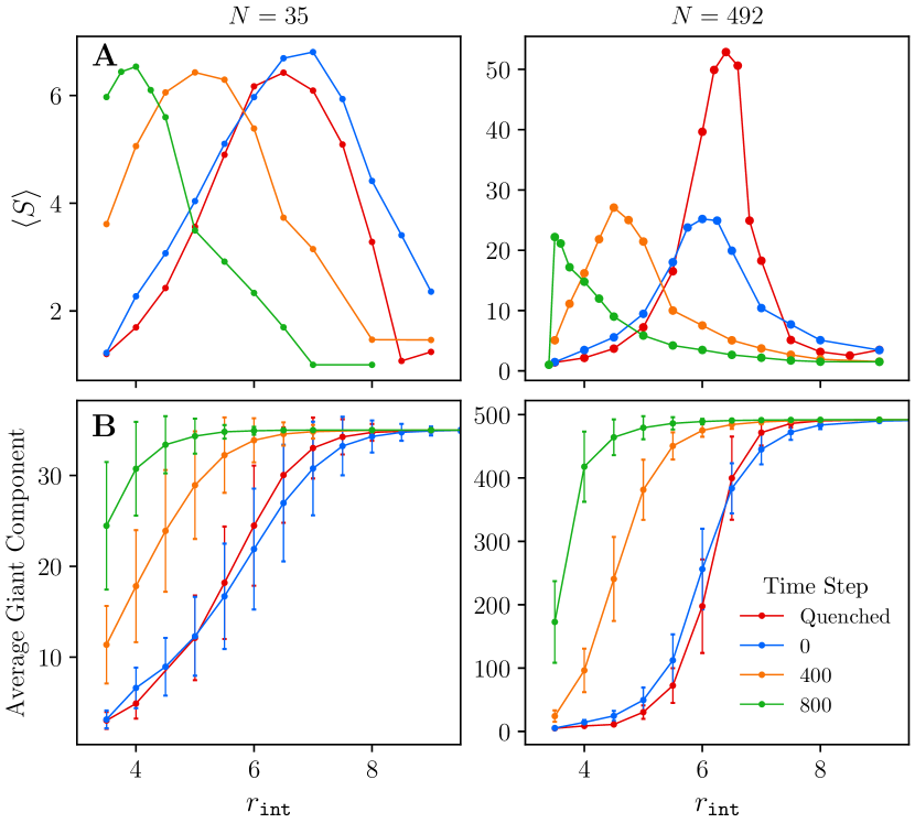
Figure 5: A: Mean cluster size and B: Average giant component as a function of the interaction radius $r_{\tt int}$ for Kilombo configurations integrated over different time-steps $\Delta t=0,400,800$ kilobot loop iterations, and for random quenched configurations. The left panel shows the results for $N=35$ kilobots, while the right panel shows results for $N=492$ kilobots and the same number density $n=0.028$ ${\tt bots}/cm^{2}$.

Figure 5 displays the mean cluster size and average giant component obtained from Kilombo simulations of kilobots as they execute PRW trajectories. Specifically, we calculate the mean cluster size characterizing their communication network integrated over the exploratory, or advertising, time window $\Delta t$. This integration considers the total number of communication contacts accumulated over the time-step $\Delta t$. We examine the communicating clusters for various time windows $\Delta t=0,400,800$ (measured in kilobot’s loop iterations) or equivalently, for $\Delta t=0,4.12$, and $8.24$ seconds, and for two different system sizes, with $N=35$ and $492$ kilobots. At this point, we want to increase the system size while maintaining a constant kilobot density, so the arena size is adjusted to keep a constant value of $n=N/\pi R^{2}=0.028$ ${\tt bots}/cm^{2}$. Later on, we will also vary the kilobot density for completeness.

The mean cluster size $\langle S\rangle$ varies with the interaction radius $r_{\tt int}$, as shown in Fig. 5A, exhibiting a peak at a threshold radius denoted by $r_{\tt int}^{*}$. For comparison and consistency check, we have included a clustering analysis for random quenched configurations of kilobots using the same sizes and density conditions. Notice that indeed the data corresponding to $\Delta t=0$ (instantaneous snapshots) closely resembles the results obtained from the quenched configurations. The small discrepancies are due to the existence of short range spatial correlations in configurations obtained from the kilobots’ dynamics, which includes collisions. Such correlations are absent in the quenched configurations.

The threshold radius $r_{\tt int}^{*}$ undergoes a notable shift towards smaller values as $\Delta t$ increases. Larger values of $\Delta t$ correspond to increasing intercommunication opportunities due to the kilobot’s advertising dynamics (see App B), and therefore to higher number of contacts in the communication network. Thus, a larger $\Delta t$ translates into a reduced percolation threshold radius, beyond which a giant communication component forms. Fig. 5B shows the average size of the giant component as a function of $r_{\tt int}$ for the same values of $\Delta t$. As the giant component approaches saturation the communication network has percolated. In particular, after an advertising time window of $\Delta t=800$ loops ($8.24$ s) in the experimental system with $N=35$ kilobots, the percolation threshold shifts from approximately $6.5\pm 0.1$ cm to $r_{\tt int}^{*}=3.75\pm 0.25$ cm, very close to the minimum distance between a kilobot pair ($r_{e}\simeq 3.3$ cm) due to excluded volume interactions.

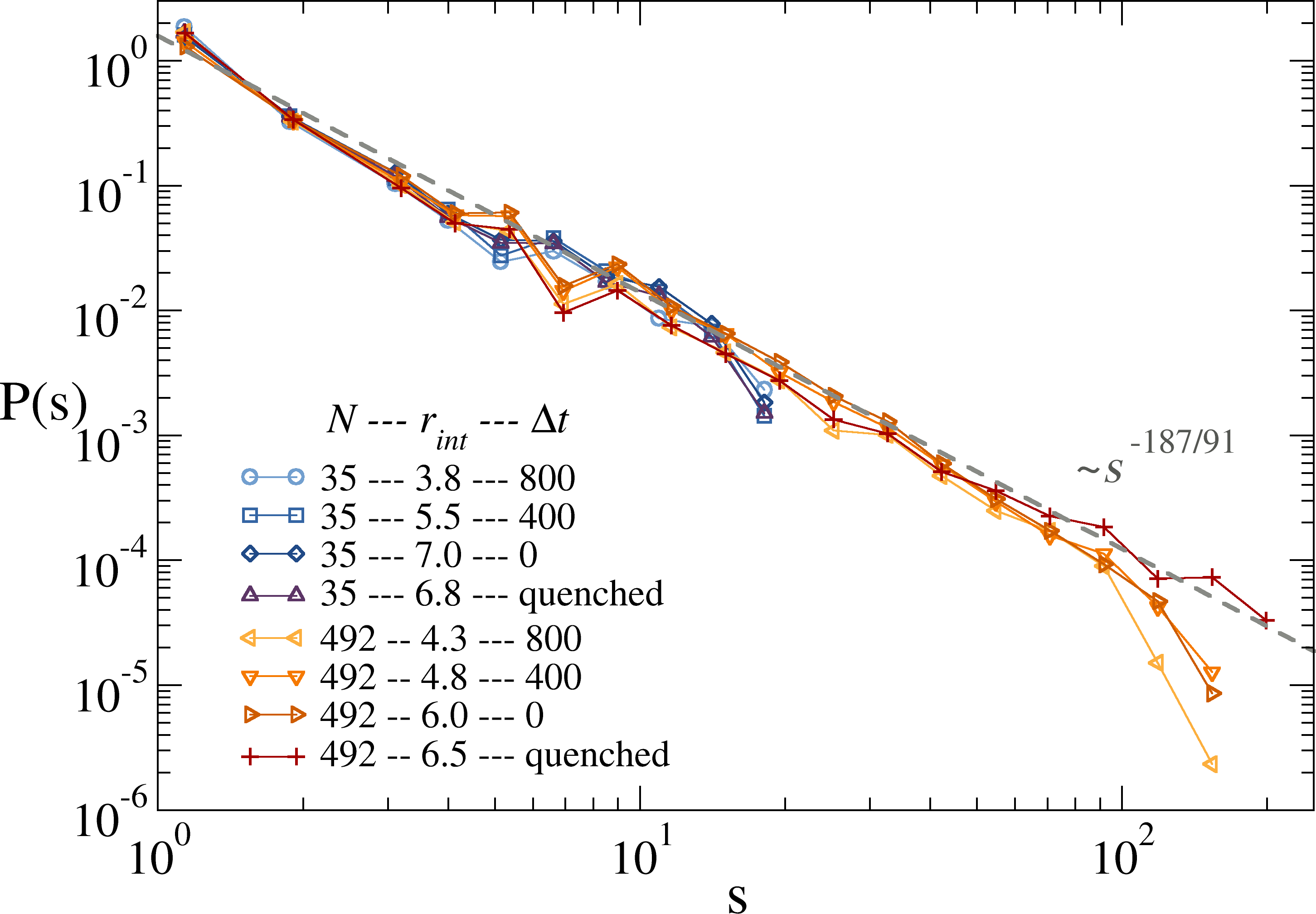
Figure 6: Probability distribution of cluster sizes $P(s)$ at the percolation transition for Kilombo and quenched kilobot simulations. The plot shows results for two system sizes with $N=35$ and $N=492$ and the same kilobot number density $n=0.028$ bots/cm². For $N=35$, the corresponding percolation thresholds are: $r_{\tt int}^{*}\simeq 3.8$ cm (Kilombo configurations integrated over $\Delta t=800$ loops), $r_{\tt int}^{*}\simeq 5.5$ cm (Kilombo configurations integrated over $\Delta t=400$ loops), $r_{\tt int}^{*}\simeq 7.0$ cm (instantaneous Kilombo configurations with $\Delta t=0$), and $r_{\tt int}^{*}\simeq 6.4$ cm (random quenched configurations). For $N=492$ one finds: $r_{\tt int}^{*}\simeq 4.3$ cm (Kilombo configurations integrated over $\Delta t=800$ loops), $r_{\tt int}^{*}\simeq 4.8$ cm (Kilombo configurations integrated over $\Delta t=400$ loops), $r_{\tt int}^{*}\simeq 6.0$ cm (instantaneous Kilombo configurations with $\Delta t=0$), and $r_{\tt int}^{*}\simeq 6.5$ cm (random quenched configurations). The gray dashed-line corresponds to a power law decay with an exponent $\tau=187/91$ characterizing the cluster distribution in $2D$ continuous percolation. It emphasizes the compatibility of our results with a percolation transition.

Interestingly, at the finite-size percolation threshold, the normalized distribution $P(s)=n(s)/n_{\text{tot}}$ of cluster sizes exhibits a power-law decay, $P(s)\sim s^{-\tau}$, persisting up to a cutoff value that depends on system size. This scaling behavior is shown in Fig. 6, where we observe a fair consistency with an exponent value $\tau\simeq 2.055$ expected for continuous percolation in $D=2$ [51]. Beyond the cutoff, the decay becomes usually much steeper.

In summary, increasing values of $\Delta t$ yield lower percolation threshold values for the pairwise interaction radius, as a result of the kilobot exploratory dynamics. By moving, bots increase their average number of communication contacts favouring the widespread of information through the system. Given that in the experimental set-up discussed in the previous section we have $N=35$ kilobots with an approximate infrared communication radius of $7$ cm, exploring their neighborhood for a time window of $\Delta t=800$ loops ($\Delta t=8.24$ s), we can conclude that the kilobot dynamics is effectively generating a percolating infrared communication network, which enables information exchange at the system-wide scale, or as in a fully-connected mean-field like scenario.

Crowding effects in consensus reaching

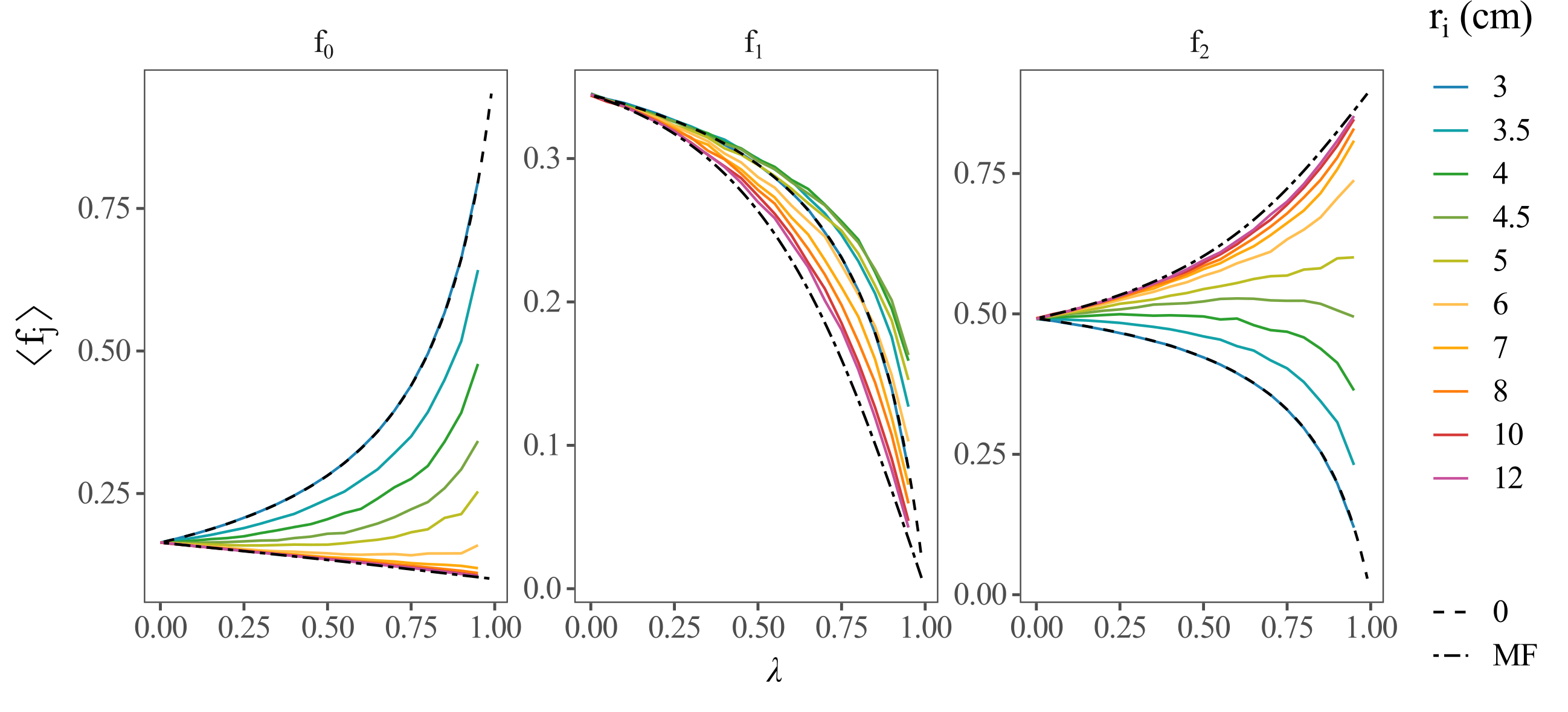
Figure 7: Stationary proportions of bots dancing for the different sites as a function of the interdependence parameter $\lambda$ for different values of the communication radius $r_{\tt int}$. Color curves correspond to simulations of the model on random quenched configurations. Dot-dashed lines show the result of the mean-field approximation, and dashed lines display the limit case of isolated bots, i.e. $r_{\tt int}=0$.

Once we understand the importance of communication among seemingly sparse and distant individuals, while they integrate remote sensing over a short temporal window as they disperse in space, we can return to the study of the main collective decision-making observables in less favorable conditions. In particular, it is now evident that the quantitative values of the dance frequencies, including uncommitted individuals ($f_{0}$) and those promoting specific sites ($f_{1}$, $f_{2}$), as well as the consensus parameter $Q$, will depend on the swarm’s effective crowding.

In this section, we explore how the number density of kilobots $n=N/\pi R^{2}$, their communication distance $r_{\tt int}$, and their sensing time $\Delta t$ influence the consensus outcome, considering different values of the interdependence parameter $\lambda$. Eventually, the dimensionless control parameter $\eta=Nr_{\tt int}^{2}/R^{2}$, measuring the effective area covered by kilobots, will determine the formation and strength of consensus as a function of the bee-like model parameters $\lambda$, $q$, and $\pi$.

To illustrate crowding effects, we start by systematically analyzing the influence of the communication range $r_{\tt int}$ on the decision-making process in the quenched configuration approximation. Figure 7 displays the stationary values of the dance frequencies $f_{0}$, $f_{1}$ and $f_{2}$ as a function of the interdependence parameter $\lambda$. The data is presented for various values of the interaction radius $r_{\tt int}\in[3,12]$ cm, represented by different colored curves. We fix the number density of kilobots to $n=0.028$ bots/cm², nest-site qualities $q_{1}=7$ and $q_{2}=10$, and independent discovery probabilities $\pi_{1}=\pi_{2}=0.3$ to match the experimental conditions. For comparison, we also include the expected stationary values in the mean-field approximation, represented by dotted-dashed lines, as well as the limiting case where bots remain completely isolated, a trivial limit of the decision making process that one can easily work-out analytically, shown as black dashed lines. The dependency of these zero-interaction curves on $\lambda$ arises from the fact that increasing $\lambda$ limits self-discovery (as one can deduce from Eq. 1) without any information exchange taking place.

For the largest interaction radius, the stationary values of $f_{j}$ tend towards the mean-field predictions. As discussed previously, beyond an interaction radius of approximately $6.5$ cm, we have a percolating communication network that allows information exchange among nearly all bots in the system. Consequently, for all interaction radii greater than this threshold ($r_{\tt int}^{*}\simeq 6.5$), the $f_{j}$ curves roughly match the mean-field results, and completely stabilize around $r_{\tt int}\sim 10$ cm. Conversely, as the interaction radius decreases from $r_{\tt int}^{*}$, the $f_{j}$ values significantly deviate from mean-field predictions, particularly for higher values of the interdependence parameter $\lambda$, when communication capabilities become crucial. When $r_{\tt int}\leq 3$ cm, due to excluded volume effects, there are no bots within the intercommunication distance (since each bot has a diameter of $3.3$ cm, touching robots cannot interact), and the stationary values of $f_{j}$ follow the isolated kilobots limit. When $\lambda=0$, the value of the interaction radius becomes irrelevant, and all curves converge to the same point, known analytically from the mean-field approximation solution of the model. The same analysis can be carried out by fixing an interaction radius $r_{\tt int}$ and changing the number of bots $N$ in a fixed-size arena. The final outcome will be the same, as it is shown in Fig. 8.

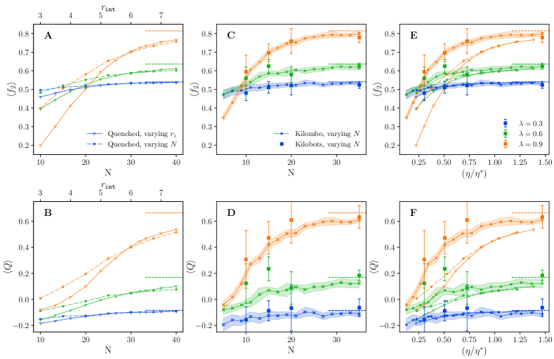
Figure 8: Stationary dance frequency for the high quality site $\langle f_{2}\rangle$ (top) and consensus parameter $\langle Q\rangle$ (bottom) as a function of the crowding control variables $N$, $r_{\tt int}$, and $\eta$. Figures A-B show results obtained from (i) different ensemble sizes $N$ and a fixed value of $r_{\tt int}=6.5$ cm (dashed-dot lines with dot symbols), (ii) from different interaction radii $r_{\tt int}$ and a constant number of $N=35$ bots (continuous lines with Y symbols), both in the quenched position approximation; Figures C-D show results obtained from (iii) Kilombo simulations (x symbols) varying $N$ and (iv) Kilobot experiments for different ensemble sizes, $N=10,\;15,\;20,\;35$ (square symbols). All simulations/experiments have been conducted for three contrasting values of the parameter $\lambda=0.3,0.6,0.9$ (blue, green and orange lines, respectively). Panels E-F show the stationary values depicted in A-B and C-D, now as a function of the percolation parameter $\eta$ rescaled by the corresponding percolation threshold $\eta^{*}$.

Finally, we investigate the impact of crowding on mobile PRW kilobots at different densities by changing the number of bots $N\in[5,35]$ in the same arena of radius $R=20$ cm. Based on the analysis presented in the previous section and in Fig. 7, we anticipate that kilobots, with the ability to move and to gather information over a temporal period $\Delta t$, will achieve better communication and consequently higher consensus levels compared to quenched configurations in the same conditions.

Figure 8 provides a comparison of stationary averaged values of $f_{2}$ and $Q$ in experiments, Kilombo simulations, and simulations using random quenched configurations. We consider three contrasting values of the interdependence parameter $\lambda$ in the symmetric probability discovery scenario. In Fig. 8A-B, we show the impact of working with different kilobot numbers $N$ or restraining their communication radius $r_{\tt int}$. Plots 8A-B show the comparison between varying $N$ or $r_{\tt int}$ in the quenched approximation. Furthermore, plots 8C-D show experimental results for varying number $N$ of kilobots contrasted with Kilombo simulations. In all cases the average values of $f_{2}$ and $Q$ increase gradually with $N$ until they reach a plateau for $N>N^{*}\sim 30$ kilobots. The plateau values lie very close to the asymptotic mean-field results for each value of $\lambda=0.3,0.6$ and $0.9$. This means that even for lower number densities than the ones considered in the experiments shown in Sec. IV (where $N=35$), the system seems to be able to perceive global information about dancing frequencies and to achieve consensus values very similar to mean-field results. This is, again, a signature of the formation of a percolating communication network as a function of kilobot density. On the contrary, the consensus parameter for very small ensemble sizes is below zero for the three contrasting values of the interdependence parameter considered, and thus strong consensus for the best quality option is not achieved in such poorly communicated swarms.

Within error bars, the stationary values of $f_{2}$ and $Q$ obtained from experiments with $N\in[5,35]$ kilobots match those from Kilombo simulations. Furthermore, moving kilobots achieve higher levels of consensus than quenched configurations with the same number of robots. This is particularly evident for small groups of kilobots and high enough values of interdependence. We have seen that the PRW motion of kilobots enhances the transmission of information and, thus, shifts the percolation transition towards smaller values of the coverage parameter $\eta$, by either decreasing the threshold value of $r_{\tt int}^{*}$ or, equivalently, by reducing the number $N^{*}$ of kilobots required to observe the percolation transition. This shift can be clearly seen by comparing Figs. 8A-B and Figs. 8C-D, for both experimental and Kilombo simulation results of moving kilobots that establish new contacts over a given time window of $\Delta t=800$ loops.

In Figs. 8E-F, the same data is now represented in terms of the dimensionless control parameter $\eta=Nr_{\tt int}^{2}/R^{2}$, measuring the effective area covered by kilobots, rescaled by the corresponding percolation threshold $\eta^{*}$ calculated in each case. Despite the rescaling by $\eta^{*}$ yields qualitatively similar dependencies on the control parameter for all the cases considered, moving kilobots slightly outperform the consensus reached in quenched conditions at high values of interdependence. This is probably due to the existence of enhanced spatial correlations below the percolation transition. Such correlations appear as a result of their characteristic dynamics, which includes the possibility of exhibiting collisions and jams and, therefore, the formation of slightly larger clusters. This fact improves the formation of strong consensus for the best quality site around the percolation transition, when $\lambda$ is high enough, as large clusters chiefly vote for the same option, enhancing $f_{2}$ while hindering $f_{1}$.

Overall, these results highlight the importance of information communication and interdependence in the kilobots’ collective decision-making process, and demonstrate the capabilities of swarm robots to successfully achieve such a complex task in far from ideal conditions. Figure 8 shows that high enough interdependence, is indeed crucial for building up strong consensus for the best-available option in poorly communicating swarms.

To conclude this section, we would like to mention that the percolation threshold is affected by finite size effects. In particular, the percolation correlation length for finite systems can only attain a maximum value

$$\xi_{max}\sim(\eta^{*}(N)-\eta^{*}_{\infty})^{-\nu}\sim N^{1/d_{f}}$$ (4)

where $\nu=4/3$ and $d_{f}=91/48$ are the critical exponents for the correlation length and the fractal dimension, respectively, for continuous percolation in $D=2$. Therefore, for the percolation threshold one expects that,

$$\eta^{*}(N)\sim\eta^{*}_{\infty}+CN^{-\frac{1}{\nu d_{f}}},$$ (5)

where $C$ is an arbitrary constant. From this expression, we expect that the percolation radius for different kilobot densities scales as

$$(r_{\tt int}^{*}(N))^{2}\sim(r_{\tt int}^{*\infty})^{2}+C^{\prime}N^{-\left(\frac{1}{\nu d_{f}}+1\right)}$$ (6)

with $(r_{\tt int}^{*\infty})^{2}\sim 0$. Indeed, in the case of quenched configurations we obtain $r_{\tt int}^{*2}\sim N^{-1.21}$, while in the case of kilobots we obtain $r_{\tt int}^{*2}\sim N^{-1.26}$ (see Supplementary Material [47]). These exponents, although slightly smaller than the continuous percolation expectation, are another indicator of a percolation process taking place in the communication network.

VI Discussion

We have investigated the problem of the nest-site selection process of honeybee swarms using kilobots, i.e. minimalist robots that can mimic their consensus-reaching behavior. Kilobots engage in a honeybee-like collective decision model while they move in the experimental arena, and we analyze how adding space and local interactions affects consensus reaching in (a simplified variant of) the model proposed by List and coworkers in 2009 [10]. In order to rationalize our experimental results, we use an analytical approach, obtained from the deterministic differential equations governing the dynamics in the mean-field approximation, as well as numerical simulations in both fully connected and random quenched kilobot configurations. Furthermore, we complement the limited statistics of our experiments with simulations using the Kilombo emulator of the kilobot dynamics. The problem of reaching consensus decisions in a decentralized manner –i.e., the need of targeting the best among many available options when many agents participate in the decision process and none of them exerts particular influence– displays great complexity and beauty and relies on information pooling and on communication. In our experiments, self-discovery and imitation, i.e. independence and interdependence, are both essential ingredients in collective decision making. We have demonstrated that kilobot swarms are capable of reaching such a complex consensus decisions collectively in a decentralized manner even in far from ideal conditions. Interestingly, we have found that the quantitative strength of this consensus not only depends on the prescriptions of independence and interdependence in the mathematical model, but also on emergent properties characterizing the swarm infrared communication network. In particular, the effective extent of individual communication capabilities and the density of kilobots play a major role, with higher coverage allowing for better communication clustering and information spread. In fact, we can associate the decision-making outcome to the system’s relative position with respect to a continuous percolation threshold, when it is seen as a complex network with bots at the nodes, and links among them if bot-to-bot message exchange is possible. We find our data for cluster size distributions and the threshold finite-size scaling to be consistent with percolation critical exponents in $D=2$. But, more importantly, the mobility of the robots -which have been scheduled to perform persistent random walks- and their time-integrated sensorial capabilities -how long they observe/advertise before taking action- completely redefine the swarm’s communication network properties. We have concluded that an effective communication coverage, which integrates all these systems variables, assumes the control of the transition and paves the way for the reaching of consensus in the social dynamics. Without the communication coverage reaching a critical threshold, the consensus is poor or nonexistent, and high enough interdependence, or imitation, turns out to be crucial for building up strong consensus for the best-available option in poorly communicating swarms. This is even more the case in asymmetric scenarios where self-discovery favors sub-optimal options.

Our study contributes to the understanding of the complexity of decentralized decision-making by interacting and moving agents, establishing the main variables to pay attention at. Simultaneously, it raises a warning on the interpretation of simple agents models solved at the mean-field level or simulated in static regular grids, when the behavior of the real insects is what we want to contrast to. We believe that swarms of mini-robots, as the kilobots here presented -or eventually, numerical emulation of their behavior-, will serve better to the end of taking into account more complex swarm properties as the bees density and hives partial coverage, their motion while communicating and their internal clocks and memory lags for listening and acting. By extensively describing their advantages and limitations, their capabilities and uncertainties, we give a recipe on how to address them as a swarm when playing a democratic game, and we hope that this will motivate further analysis and exploration on mini-robots as programmable social matter.

Appendix A Methods

A.1 Deterministic solutions of the Mean Field Model

In Ref. [36], T. Galla provided an analytical approach to List et al. model using a simple alteration of the original model. As mentioned in the main text, Galla replaces the state variables $(s_{i,t},d_{i,t})$ by $s_{i,t}$, and introduces a dance abandonment rate $r_{j}$ for each site such that $<r_{j}>\sim q_{j}^{-1}$. Following the mathematical details provided in [36] one can arrive to a set of deterministic differential equations that describe the time evolution of the system. For each site $j=1,...,k$:

$$\langle\dot{f}_{j,t}\rangle=(1-\rho(t))[(1-\lambda)\pi_{j}+\lambda\langle f_{j,t}\rangle]-r_{j}\langle f_{j,t}\rangle$$ (7)

where $\rho(t)=\sum_{\alpha=1}^{k}\langle f_{\alpha,t}\rangle$. Eq. 7 can be numerically integrated for any fixed choice of parameters. Nevertheless, an expression for the stationary points of these equations can be found as the solution of $k$ coupled quadratic equations, obtained by setting $\langle\dot{f}_{j,t}\rangle=0$

$$f^{*}_{j}=\biggr{[}\frac{r_{j}}{1-\rho^{*}}-\lambda\biggr{]}^{-1}(1-\lambda)\pi_{j}\quad j=1,...,k.$$ (8)

In order to solve this system of equations, that unavoidably depends on the stationary value $1-\rho^{*}=f_{0}^{*}$, one can combine the $k$ equations to solve first a closed equation for $f_{0}^{*}$:

$$f^{*}_{0}=1-(1-\lambda)\sum^{k}_{j=1}\biggr{[}\frac{r_{j}}{f^{*}_{0}}-\lambda\biggr{]}^{-1}\pi_{j}.$$ (9)

Eq. 9 has $k+1$ roots that can be found by solving the equation numerically or by rearranging it as a $(k+1)$-th degree polynomial in $f_{0}$. Some of these roots lead to unphysical solutions with $f^{*}_{0}>1$. From the remaining valid solutions with $f_{0}^{*}\leq 0$, only one leads to valid ($f^{*}_{j}\leq 1$) and linearly stable solutions for the rest of dance frequencies. Stochastic simulations and the integration of Eq. 7 confirm the stability of this result.

The extreme cases $\lambda=0$ and $\lambda\rightarrow 1$ have simpler solutions. First, setting $\lambda=0$ in Eq. 9 leads to a simpler solution,

$$f_{0}^{*}=\frac{1}{1+\sum_{m=1}^{k}\pi_{m}q_{m}},$$ (10)

that we can use to compute the result for the rest of the dancing frequencies. Using Eq. 8, we obtain

$$f_{j}^{*}=\frac{\pi_{j}q_{j}}{1+\sum_{j=m}^{k}\pi_{m}q_{m}}.$$ (11)

When $\lambda\rightarrow 1$ ($\lambda=1$ is an ill-defined case where the dynamics of the system remains the same for any value the discovery probabilities $\pi_{j}$’s since self-discovery information won’t be introduced in the swarm through the term $(1-\lambda)\pi_{j}$), due to the extreme reliance on interdependence, one expects that the site with a greater quality will be finally dominating the whole system, leaving no agents committed to the other sites and only a small quantity of uncommitted agents. Assuming that $q_{k}>q_{k-1}>...>q_{1}$, we can impose that $f_{1}^{*}=...=f_{k-1}^{*}=0$, and using 8 we find the following stationary solution:

$$f_{0}^{*}=r_{k},\quad f_{1}^{*}=...=f_{k-1}^{*}=0,\quad f_{k}^{*}=1-r_{k}.$$ (12)

This result is validated by simulations, or after solving the deterministic equations at high values of $\lambda$. A linear stability analysis confirms that this solution is the only stable solution in the limit $\lambda\rightarrow 1$ [48].

A.2 Kilobots experimental set-up

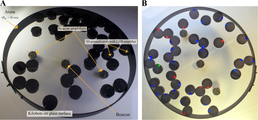
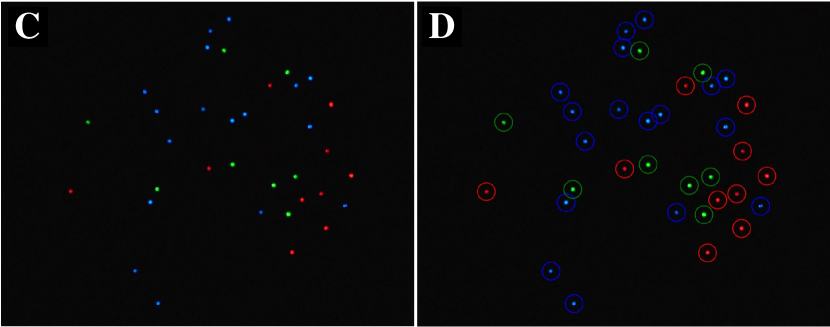
Figure A1: A: Kilobots experimental setup. B: Kilobots dynamics as described in Sec. II (see video in [47]). Each kilobot is covered by a custom 3D-printed case than enhances visual on the led light and allows for tracking. C: A single frame showcasing a group of $35$ kilobots, each identified by their colored light, dancing for site one (green), site two (blue), or not dancing for any site (red). D: The frame in C processed using the kilocounter software.

Kilobots have been instrumental in collective behavior research [37]. Kilobots execute user-programmed functions in loops, and the loop duration varies based on the complexity of the operations. In our case, kilobots perform a persistent random walk (PRW) while gathering information, estimating population frequencies, computing transition probabilities, and indicating their commitment state during each loop. For our experiments, we set up a workspace with kilobots moving on a glass surface held $15$ cm above a whiteboard melamine base. On the melamine base, we place a central kilobot that acts as a beacon to enhance synchronization of the kilobots’ internal clocks, alongside two additional kilobots that amplify the beacon signal. Our typical setup is illustrated in Fig. A1-A. Synchronization is important to coordinate concurrent processes, such as those involved in the collective decision model.

Groups of $10$ to $35$ kilobots move as PRWs in a circular arena with a $20$ cm radius. After transmitting and receiving messages, and gathering information from their local environment, during a time-step $\Delta t$, typically $800$ loop iterations or approximately $8.24$ seconds , kilobots update their state according to the model dynamics, and consequently ‘dance for’ either site 1 (low quality), site 2 (high quality), or for no site, displaying such individual state in their LED (red for non-dancing, green if dancing for site 1, and blue if dancing for site 2).

To prevent our group of kilobots from clustering at the wall of the circular observation area, their random dynamics was configured with discrete wide turning angles to promote quicker turning away from the border. Turning times consist of approximately $\sim 2.8$ seconds ($125^{\circ}$) or $\sim 5.8$ seconds ($251^{\circ}$), and their moving forward states last approximately $\sim 3.8$ seconds. To better identify the kilobots’ states, we covered each kilobot with a custom 3D-printed black casing, leaving only the LED light visible, as seen in Fig. A1-B.

We recorded the kilobots dynamics and LED states using a digital camera with a spatial resolution of $1920x1080$ pixels and a temporal resolution of $25$ frames per second. Each recording session lasts typically 30 minutes. To automatically count the number of kilobots dancing for each site, we extract images at each time step $\Delta t$, and we make use of the kilocounter software, specifically developed for our work [52]. Kilocounter identifies and counts colored blobs in these recordings, allowing us to analyze kilobot behavior, as shown in Fig. A1C-D. To facilitate the tracking, videos are recorded in a dark setting.

Table 1: Number of realizations of the kilobot experiments for each experimental condition defined by $N$ and $\lambda$.

	10	15	20	35
$\mathbf{0.3}$	10	6	5	5
$\mathbf{0.6}$	10	7	5	5
$\mathbf{0.9}$	10	5	5	5

Table 1 sums up the amount of experiments conducted for each condition, defined by the system size $N$ and the interdependence parameter $\lambda$. Due to the time consuming process of conducting the experiments, the number of realizations is limited.

Appendix B Complementary analysis on kilobots behavior: Kilobots detected over a time-step

In the study of opinion dynamics, understanding how individuals interact to make decisions is crucial. Kilobots gather information from their neighbors and then act accordingly. We want to know how many other bots are detected by a kilobot during a time-step.

We thus implement an algorithm for a bot to communicate, at each time-step, the number of bots seen over the previous time-step. We will run this algorithm on uncommitted, non-dancing bots, while the dancing bots (promoting either site $1$ or site $2$) perform PRWs. First, we check that the maximum number of kilobots detected by an uncommitted bot (during a time-step $\Delta t=800$ loops) is around $15$, in the 20 cm arena with 35 kilobots running the nest-site selection model. We restrict the count to bots seen within an interaction radius of $\sim 7$ cm, about $2$ kilobots’ body lengths. This is possible by filtering for the infrared signal intensity. We then divide the number of bots detected during a time-step $\Delta t$ in four intervals, and assign each interval a color: red ($0-3$ bots), green ($4-7$ bots), blue ($8-11$ bots) and white ($12-15$ bots). At each time step, uncommitted bots flush their LEDs according to this color code, and we count the numbers with the kilocounter software. We perform five repetitions of $210$ time-steps (about $30$ minutes each) to gather statistics (over $\sim 20000$ counts).

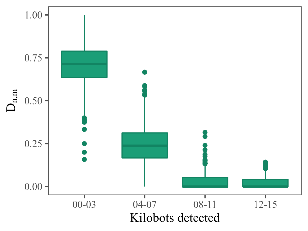
Figure A2: Kilobots detected over a time step $\Delta t$ in experiments. The boxplots show the proportion of kilobots detecting from $n$ to $m$ neighbors for four different $(n,m)$ ranges.

Figure A2 shows in a boxplot the ratio $D_{n,m}$, which represents the proportion of kilobots detecting from $n$ to $m$ neighbor kilobots during $\Delta t$. Most kilobots only detect $0-3$ other bots, or $4-7$, during a time step. In other words, undecided bots detect on average $2.92\pm 2.50$ bots during each $\Delta t$.

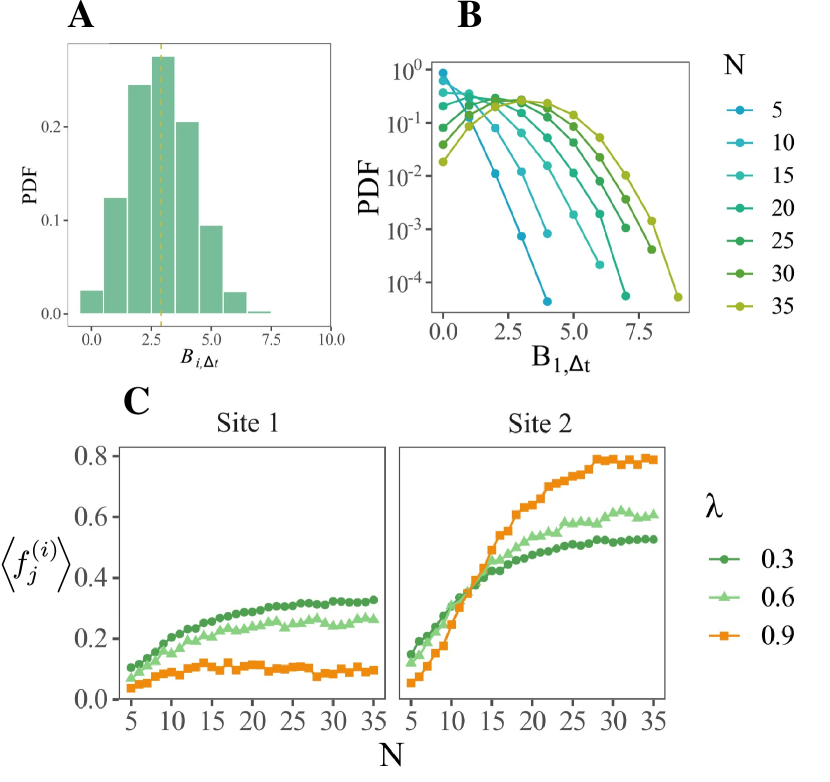
Figure A3: Kilobots detected during a time-step $\Delta t$ in Kilombo. A: Probability distribution, $B_{i,\Delta t}$, of kilobots detected by a focal kilobot $i$ in a time-step $\Delta t$. B: Same as A in logscale and for different number $N$ of kilobots in the arena. C: Average ratio of kilobots dancing for site $j$ detected by a focal kilobot $i$ in a time-step $\Delta t$, $f^{(i)}_{j}$, as a function of the number $N$ of kilobots in the arena, for three different values of $\lambda$.

Additionally, we used the Kilombo simulator, confirming that the number of kilobots detected per $\Delta t$ was consistent with our experimental results. Figure A3A shows the distribution of bots detected by a focal kilobot $i$ in $\Delta t$, $B_{i,\Delta_{t}}$. Uncommitted bots in Kilombo detected a mean of $2.91\pm 1.35$ bots. With the reassurance that Kilombo fairly mimics quantitatively the real system, we also analyze how the number of bots seen vary when varying the kilobot density. Figure A3B shows the distribution $B_{i,\Delta_{t}}$ as the number of kilobots $N$ goes from $N=5$ until $N=35$. As $N$ increases, curves shift towards the right but, in all cases, the average $B_{i,\Delta_{t}}$ remains below 5.

The emulator also provides more detailed information about the proportions of detected bots that were dancing for each site. We analyze the ratio of kilobots seen by the focal kilobot $i$ separating those dancing for each available site $j$, $f^{(i)}_{j}$, during $\Delta t$ for three contrasting values of the interdependence parameter $\lambda$. In Fig. A3C, we represent the average $\langle f^{(i)}_{j}\rangle$ for $j=1,2$ as $N$ is increased, for $\lambda=0.3,0.6,0.9$. We observe that the $\langle f^{(i)}_{j}\rangle$ increase gradually with $N$ until they reach a plateau for a group of approximately $30$ kilobots. As we discuss in the main text, this feature corroborates the existence of a percolating communication network.

Appendix C Complementary analysis of the communication network

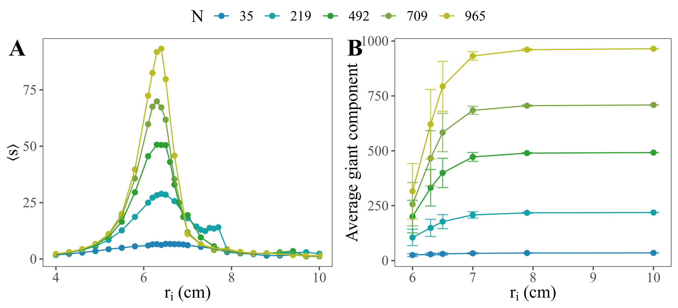
Figure A4: A: Mean cluster size, and B: Average giant component as a function of the communication radius $r_{\tt int}$ for quenched configurations on different system sizes that preserve the same number density. Cluster sizes were averaged over $1000$ configurations per system size.

C.1 Finite-size scaling in quenched configurations

Here we provide a complementary finite-size scaling analysis of communicating cluster formation in quenched configurations of bots randomly located on a circular arena. In Figure A4A, we plot the mean-cluster size $\langle S\rangle$ for different system sizes, preserving the same number density $N/\pi R^{2}=0.028$ bots$/cm^{2}$, as a function of the communication radius $r_{\tt int}$, which characterizes the maximum extent of message transmission, and thus of information exchange, through infrared sensors among physical kilobots. We can identify the critical percolation interaction radius at around $r_{\tt int}^{*}=6.5\pm 0.2$ cm.

Continuous percolation threshold values for two dimensional discs of effective radius $r_{\tt int}$ in a square box of linear dimension $L$ with periodic boundary conditions are found in the literature [53]. The critical filling factor in that particular geometry is $\eta^{*}=N\pi r_{\tt int}^{2}/L^{2}\simeq 1.128$, or equivalently, $r_{\tt int}^{*}=(L^{2}\eta^{*}/(N\pi))^{1/2}$. Assuming a similar scaling behavior in our case, with a fixed rigid circular wall, would yield a smaller threshold radius of approximately $3.59$ cm, indicating that both our circular geometry and fixed boundary conditions give rise to packing and size effects that cannot be neglected in the quantitative determination of this non-universal threshold value. On the other hand, such effects should not be relevant regarding the behavior of critical exponents.

In Figure A4B, we represent the average size of the giant component (the largest connected cluster in the system) as a function of the interaction radius $r_{\tt int}$. This quantity attains its maximum value, comparable to the system size, after the percolation threshold. As the maximum value of the mean cluster size, the size of the giant component at the percolation threshold scales as a power-law of the system size.

C.2 Communication network degree distribution

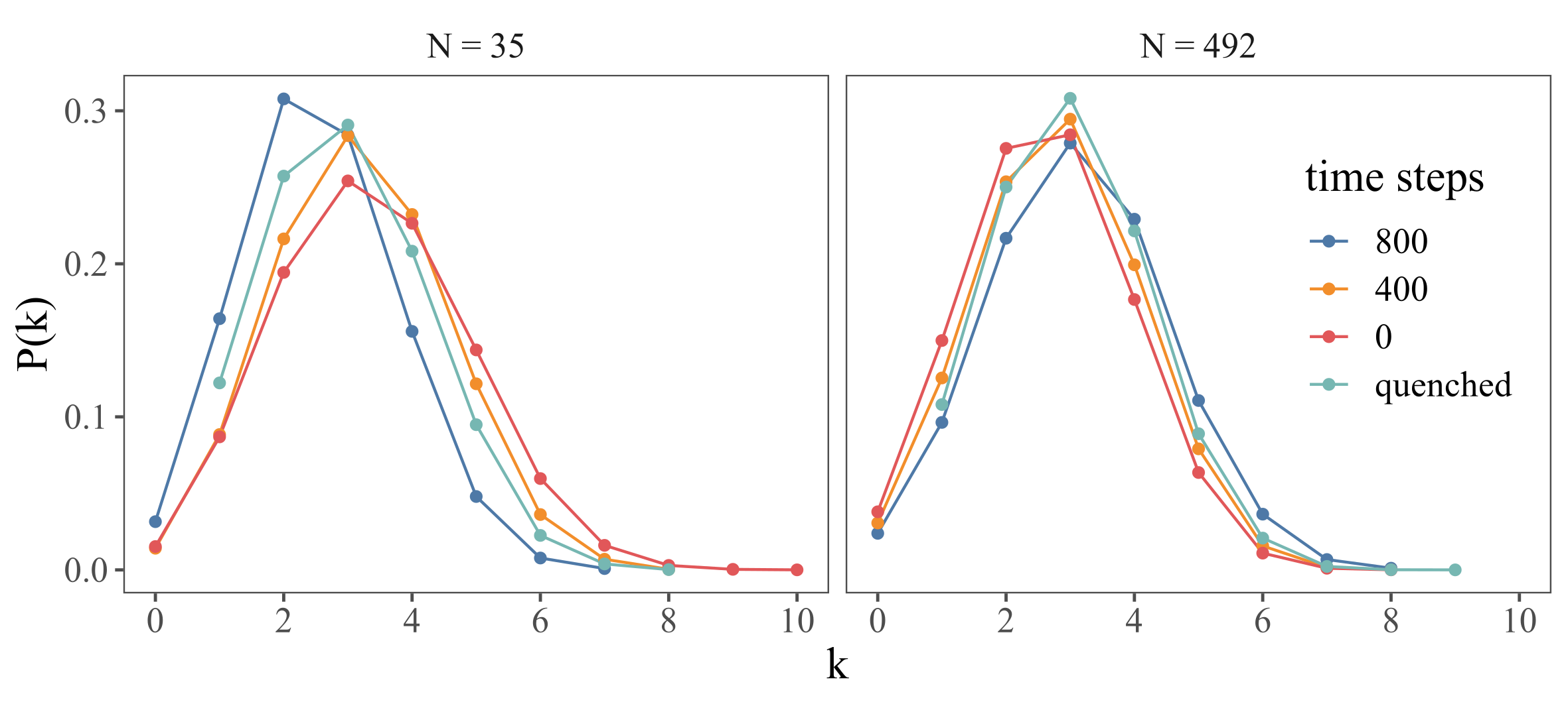
Figure A5: Top: Degree distribution $P(k)$ at the percolation threshold $r_{\tt int}^{*}$. Data obtained from Kilombo simulations integrating over different time-steps, $\Delta t=0,400,800$ loop iterations and for $1000$ quenched bot configurations. Bottom: Degree distributions obtained for different interaction radius $r_{\tt int}$ and a fixed value of $\Delta t=800$ loop iterations. Left panels correspond to $N=35$, and right panels to $N=495$.

In network theory, a node’s degree $k$ represents its number of connections with other nodes, while the degree distribution $P(k)$ indicates the probability of a randomly chosen node having degree $k$ [49]. Both degree and degree distribution are crucial for understanding dynamic processes on networks, such as information spread in the kilobots’ infrared communication network.

Figure A5 illustrates the degree distribution observed for the communication network built-up in Kilombo simulations after integrating over various exploratory time-steps ($\Delta t$). Two different system sizes with the same kilobot number density are considered. The bell-shaped curves roughly resemble a Poisson distribution ($P(k)=e^{-\lambda}\frac{\lambda^{k}}{k!}$), where $\lambda$ represents the average degree $\langle k\rangle$.

Additionally, we compute the average degree ($\langle k\rangle$) of the communication network integrated over different $\Delta t$ values in Kilombo simulations and for quenched random configurations, and the same system sizes ($N=35$ and $N=492$).

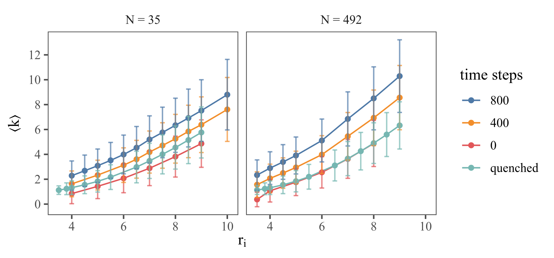
Figure A6: Average degree $\langle k\rangle$ of the communication network as a function of $r_{\tt int}$. Results are obtained from Kilombo simulations integrating over different time steps $\Delta t=0,400,800$ loop iterations, and for $1000$ quenched configurations. Left panel: $N=35$. Right panel: $N=495$.

Figure A6 shows $\langle k\rangle$ as a function of $r_{\tt int}$ for the same time windows. Increasing $\Delta t$ and/or interaction radius $r_{\tt int}$ results in higher values of $\langle k\rangle$, which eventually overcome the threshold average degree $\langle k\rangle^{*}=1$ required for the presence of a giant component in this network according to the celebrated Molloy and Reed criterion [54]. These findings align with a network interpretation of the percolation transition.

For the smaller system ($N=35$), quenched kilobot configurations exhibit a slightly larger average degree compared to single snapsholts of Kilombo simulations ($\Delta t=0$), potentially due to the accumulation of some bots at the arena wall. This effect diminishes for the larger system size, yielding similar $\langle k\rangle$ values for both quenched and $\Delta t=0$ configurations.

References

- Bose et al. [2017] T. Bose, A. Reina, and J. A. Marshall, Current Opinion in Behavioral Sciences 16, 30 (2017).
- Dyer et al. [2009] J. R. Dyer, A. Johansson, D. Helbing, I. D. Couzin, and J. Krause, Philosophical Transactions of the Royal Society B: Biological Sciences 364, 781 (2009).
- Sasaki and Pratt [2018] T. Sasaki and S. C. Pratt, Annual Review of Entomology 63, 259 (2018).
- von Frisch [1954] K. von Frisch, The dancing bees (Springer Vienna, 1954).
- Seeley [2010] T. D. Seeley, in Honeybee Democracy (Princeton University Press, 2010).
- Couzin et al. [2005] I. D. Couzin, J. Krause, N. R. Franks, and S. A. Levin, Nature 433, 513 (2005).
- Dong et al. [2023] S. Dong, T. Lin, J. C. Nieh, and K. Tan, Science 379, 1015 (2023).
- Britton et al. [2002] N. F. Britton, N. R. Franks, S. C. Pratt, and T. D. Seeley, Proceedings of the Royal Society of London. Series B: Biological Sciences 269, 1383 (2002).
- Passino and Seeley [2006] K. M. Passino and T. D. Seeley, Behavioral Ecology and Sociobiology 59, 427 (2006).
- List et al. [2009] C. List, C. Elsholtz, and T. D. Seeley, Philosophical Transactions of the Royal Society B: Biological Sciences 364, 755 (2009).
- Pais et al. [2013] D. Pais, P. M. Hogan, T. Schlegel, N. R. Franks, N. E. Leonard, and J. A. R. Marshall, PLOS ONE 8, 1 (2013).
- Reina et al. [2017] A. Reina, J. A. R. Marshall, V. Trianni, and T. Bose, Phys. Rev. E 95, 052411 (2017).
- Cavagna et al. [2010] A. Cavagna, A. Cimarelli, I. Giardina, G. Parisi, R. Santagati, F. Stefanini, and M. Viale, Proceedings of the National Academy of Sciences 107, 11865 (2010).
- Rosenthal et al. [2015] S. B. Rosenthal, C. R. Twomey, A. T. Hartnett, H. S. Wu, and I. D. Couzin, Proceedings of the National Academy of Sciences 112, 4690 (2015).
- Chen et al. [2016] D. Chen, T. Vicsek, X. Liu, T. Zhou, and H.-T. Zhang, Europhysics Letters 114, 60008 (2016).
- Calovi et al. [2018] D. S. Calovi, A. Litchinko, V. Lecheval, U. Lopez, A. Pérez Escudero, H. Chaté, C. Sire, and G. Theraulaz, PLOS Computational Biology 14, 1 (2018).
- Múgica et al. [2022] J. Múgica, J. Torrents, J. Cristín, A. Puy, M. C. Miguel, and R. Pastor-Satorras, Scientific Reports 12, 10783 (2022).
- Valentini et al. [2017] G. Valentini, E. Ferrante, and M. Dorigo, Frontiers in Robotics and AI 4 (2017).
- Garnier et al. [2009] S. Garnier, J. Gautrais, M. Asadpour, C. Jost, and G. Theraulaz, Adaptive Behavior 17, 109 (2009).
- Schmickl et al. [2007] T. Schmickl, C. Möslinger, and K. Crailsheim, in Swarm Robotics, edited by E. Şahin, W. M. Spears, and A. F. T. Winfield (Springer Berlin Heidelberg, Berlin, Heidelberg, 2007) pp. 144–157.
- Valentini et al. [2014] G. Valentini, H. Hamann, and M. Dorigo, in Proceedings of the 2014 International Conference on Autonomous Agents and Multi-Agent Systems, AAMAS ’14 (International Foundation for Autonomous Agents and Multiagent Systems, Richland, SC, 2014) p. 45–52.
- Holley and Liggett [1975] R. A. Holley and T. M. Liggett, The Annals of Probability 3, 643 (1975).
- Castellano et al. [2009] C. Castellano, S. Fortunato, and V. Loreto, Rev. Mod. Phys. 81, 591 (2009).
- Galam, S. [2002] Galam, S., Eur. Phys. J. B 25, 403 (2002).
- Galam [2008] S. Galam, International Journal of Modern Physics C 19, 409 (2008).
- Deffuant et al. [2000] G. Deffuant, D. Neau, F. Amblard, and G. Weisbuch, Advances in Complex Systems 03, 87 (2000).
- Johnstone [1997] R. A. Johnstone, Behavioural ecology: An evolutionary approach 155178 (1997).
- Far [2020] Data-Driven Modeling of Resource Distribution in Honeybee Swarms, ALIFE 2023: Ghost in the Machine: Proceedings of the 2023 Artificial Life Conference, Vol. ALIFE 2020: The 2020 Conference on Artificial Life (2020).
- Seeley et al. [2012] T. D. Seeley, P. K. Visscher, T. Schlegel, P. M. Hogan, N. R. Franks, and J. A. R. Marshall, Science 335, 108 (2012).
- Beekman and Oldroyd [2018] M. Beekman and B. P. Oldroyd, Philosophical Transactions of the Royal Society B: Biological Sciences 373, 20170010 (2018).
- Seeley and Buhrman [2001] T. D. Seeley and S. C. Buhrman, Behavioral Ecology and Sociobiology 49, 416 (2001).
- Dyer [2002] F. C. Dyer, Annual Review of Entomology 47, 917 (2002).
- Seeley [1997] T. D. Seeley, The American Naturalist 150, S22 (1997).
- Myerscough [2003] M. R. Myerscough, Proceedings of the Royal Society of London. Series B: Biological Sciences 270, 577 (2003).
- Perdriau and Myerscough [2007] B. S. Perdriau and M. R. Myerscough, Biology Letters 3, 140 (2007).
- Galla [2010] T. Galla, Journal of Theoretical Biology 262, 186 (2010).
- Rubenstein et al. [2012] M. Rubenstein, C. Ahler, and R. Nagpal, in 2012 IEEE International Conference on Robotics and Automation (2012) pp. 3293–3298.
- Valentini et al. [2016] G. Valentini, E. Ferrante, H. Hamann, and M. Dorigo, Autonomous Agents and Multi-Agent Systems 30, 553 (2016).
- Gauci et al. [2018] M. Gauci, R. Nagpal, and M. Rubenstein, Programmable self-disassembly for shape formation in large-scale robot collectives, in Distributed Autonomous Robotic Systems: The 13th International Symposium, edited by R. Groß, A. Kolling, S. Berman, E. Frazzoli, A. Martinoli, F. Matsuno, and M. Gauci (Springer International Publishing, Cham, 2018) pp. 573–586.
- Slavkov et al. [2018] I. Slavkov, D. Carrillo-Zapata, N. Carranza, X. Diego, F. Jansson, J. Kaandorp, S. Hauert, and J. Sharpe, Science Robotics 3, eaau9178 (2018).
- Dimidov et al. [2016] C. Dimidov, G. Oriolo, and V. Trianni, in Swarm Intelligence, edited by M. Dorigo, M. Birattari, X. Li, M. López-Ibáñez, K. Ohkura, C. Pinciroli, and T. Stützle (Springer International Publishing, Cham, 2016) pp. 185–196.
- Rubenstein et al. [2013] M. Rubenstein, A. Cabrera, J. Werfel, G. Habibi, J. McLurkin, and R. Nagpal, in Proceedings of the 2013 International Conference on Autonomous Agents and Multi-Agent Systems, AAMAS ’13 (International Foundation for Autonomous Agents and Multiagent Systems, Richland, SC, 2013) p. 47–54.
- Zion et al. [2023] M. Y. B. Zion, J. Fersula, N. Bredeche, and O. Dauchot, Science Robotics 8, eabo6140 (2023).
- Jansson et al. [2016] F. Jansson, M. Hartley, M. Hinsch, I. Slavkov, N. Carranza, T. S. G. Olsson, R. M. Dries, J. H. Grönqvist, A. F. M. Marée, J. Sharpe, J. A. Kaandorp, and V. A. Grieneisen, Kilombo: a kilobot simulator to enable effective research in swarm robotics (2016), arXiv:1511.04285 [cs.RO] .
- Sumpter [2006] D. Sumpter, Philosophical Transactions of the Royal Society B: Biological Sciences 361, 5 (2006).
- Judd [1994] T. M. Judd, Journal of Insect Behavior 8, 343 (1994).
- [47] URL_will_be_inserted_by_publisher, supplementary material for this work which contains videos of our experiments.
- Pons et al. [2023] D. M. Pons, E. E. Ferrero, and C. Miguel, Parametric exploration of the honeybees nest-site choice problem, In preparation (2023).
- Newman [2010] M. Newman, Networks: An Introduction (Oxford University Press, Inc., USA, 2010).
- Barthélemy [2011] M. Barthélemy, Physics Reports 499, 1 (2011).
- Stauffer and Aharony [2018] D. Stauffer and A. Aharony, Introduction to percolation theory (Taylor & Francis, 2018).
- [52] Kilocounter, https://github.com/ivan-paz/kiloColors/blob/main/RGBKiloCounter/, blob detection and color counting software.
- Mertens and Moore [2012] S. Mertens and C. Moore, Phys. Rev. E 86, 061109 (2012).
- Molloy and Reed [1995] M. Molloy and B. Reed, Random Structures & Algorithms 6, 161 (1995).