Mean-square Exponential Stabilization of
Mixed-autonomy Traffic PDE System

Abstract

Control of mixed-autonomy traffic where Human-driven Vehicles (HVs) and Autonomous Vehicles (AVs) coexist on the road have gained increasing attention over the recent decades. This paper addresses the boundary stabilization problem for mixed traffic on freeways. The traffic dynamics are described by uncertain coupled hyperbolic partial differential equations (PDEs) with Markov jumping parameters, which aim to address the distinctive driving strategies between AVs and HVs. Considering the spacing policies of AVs vary in the mixed traffic, the stochastic impact area of AVs is governed by a continuous Markov chain. The interactions between HVs and AVs such as overtaking or lane changing are mainly induced by the impact areas. Using backstepping design, we develop a full-state feedback boundary control law to stabilize the deterministic system (nominal system). Applying Lyapunov analysis, we demonstrate that the nominal backstepping control law is able to stabilize the traffic system with Markov jumping parameters, provided the nominal parameters are sufficiently close to the stochastic ones on average. The mean-square exponential stability conditions are derived, and the results are validated by numerical simulations.

, , ,

1 Introduction

Stop-and-go traffic oscillations, as common traffic instabilities on freeways, lead to increased travel time, fuel consumption, and the risk of traffic accidents. Stabilization of stop-and-go traffic is mainly achieved via traffic management infrastructures such as ramp metering and varying speed limits. The rapid development of Autonomous Vehicles (AVs) over the recent years has brought an increasing market penetration rate of AVs on road [12]. It was initially envisioned that AVs could operate with minimal vehicle following distances, potentially leading to increased road capacity. This notion has been explored through both theoretical modeling and field experiments [18, 25]. However, it is noteworthy that current commercially available AVs may maintain longer distance headways than Human-driven Vehicles (HVs). This is primarily due to safety considerations, as AVs require a sufficient safety buffer to react effectively in the risky event such as the preceding vehicle comes to a complete stop [23].

Macroscopic modeling for pure HV traffic can be represented by Lighthill and Whitham and Richard (LWR) model [24, 31], and the Aw-Rascle-Zhang(ARZ) model [7, 39]. Among these, the ARZ model is widely adopted for its ability to describe the stop-and-go oscillations, compared to the LWR. The ARZ model comprises coupled first-order hyperbolic PDEs, which describes the evolution of traffic density and velocity states. To stabilize traffic at its equilibrium, numerous studies have attempted to address the stabilization problem using boundary backstepping control [3, 16, 20, 33, 38]. In [37, 38] the authors first proposed boundary feedback control laws to reduce traffic oscillations in congested regimes, developing full-state feedback and output feedback control laws to achieve exponential stability of the linearized ARZ model. However, they did not consider system disturbance and other noise. PI boundary controllers [41] is also applied to stabilize the traffic system described by PDEs around the given steady state. Considering disturbances and measurement noise in the hyperbolic system, the authors in [5, 21] designed robust output feedback regulation to ensure system robustness against delays and uncertainties. In addition, distributed control schemes also play a crucial role in the stabilization of PDE traffic systems. Bekiaris-Liberis [9] proposed a control law to stabilize traffic flow for an ARZ-type model consisting of both adaptive cruise control(ACC)-equipped and manually driven vehicles. The authors in [29] further considered the input delay and developed an input delay-compensating control law to stabilize mixed traffic scenarios.

The traffic models for general one-class vehicles are not valid when the road is made up of more than one traffic participant. Considering the multi-class vehicles on the road, Mohan [26] proposed a continuum model using the concept of area occupancy for mixed-autonomy traffic and calibrated the established speed-AO relation using experimental data. Burkhardt [11] adopted this speed-AO relation to describe the interaction between two-class vehicles and developed full-state feedback control laws and output-feedback control laws using backstepping technology to achieve exponential stability in $L_{2}$-sense. However, they are dealing with the deterministic condition of the mixed autonomy traffic system. Real-world traffic systems are influenced by various stochastic factors such as random vehicle arrival rates and diverse driving behaviors among vehicle types [1, 17, 27]. These factors cause deterministic systems to become stochastic, with random parameters embedded within the system.

To stabilize the oscillations of the stochastic mixed autonomy traffic system, we propose in this paper a mean-square exponential control method. The stability of stochastic linear hyperbolic PDEs has been widely investigated [2, 10, 13, 22, 28]. Prieur [28] modeled the abrupt changes of boundary conditions as a piecewise constant function and derived sufficient conditions for exponential stability of the switching system. Wang et al. [34] examined the robustly stochastically exponential stability and stabilization of uncertain linear first-order hyperbolic PDEs with Markov jumping parameters, deriving sufficient stability conditions using linear matrix inequalities (LMIs) based on integral-type stochastic Lyapunov functional (ISLF). Auriol [6] demonstrated the mean-square exponential stability of coupled hyperbolic systems with Markovian parameters. With further applications in traffic flow, Zhang [40] studied traffic flow control of Markov jump hyperbolic systems, employing LMI to derive sufficient conditions for exponential stability. The stability of mixed-autonomy traffic containing CAV platoons and HVs with two-mode Markov jump parameters was analyzed, and sufficient conditions for the stochastic system’s stability were established [36]. However, there is a scarcity of results on the stabilization of stochastic mixed-autonomy traffic systems. In this paper, we consider a nominal boundary controller designed with the backstepping method. Provided the nominal parameters are sufficiently close to the stochastic ones on average, this control law will stabilize the stochastic mixed-autonomy traffic system.

The main results of this paper are that we first propose a stochastic mixed-autonomy traffic PDE system with the stochastic disturbance of AVs governed by the Markov process. On the other hand, we design a backstepping boundary control law that achieves mean-square stabilization of the traffic system with the Markov-jumping parameters. The significance of this paper extends to both theoretical advancements and practical applications. We develop a backstepping control methodology for mean-square stabilization of coupled hyperbolic PDEs with stochastic parameters. To the best of the authors’ knowledge, this represents the inaugural application result on the stabilization of stochastic mixed-autonomy traffic.

The paper is organized as follows: In Section 2, the stochastic factors in mixed-autonomy traffic systems are considered and thus the stochastic mixed-autonomy traffic model is developed. Section 3 defines the nominal case of the stochastic traffic system. The backstepping control law for the nominal system is designed and the Lyapunov analysis for the nominal system is applied to prove the stability of the nominal system. The well-posedness of the stochastic system under the control law is also proved. Section 4 provides a Lyapunov analysis of the stochastic mixed autonomy traffic system and derives sufficient conditions for the mean-square exponential stability of the system. Numerical simulation results validating the theoretical derivations are presented in Section 5. Finally, Section 6 concludes the paper.

2 Stochastic mixed-autonomy traffic model

In this section, we present the extended stochastic ARZ model that describes the mixed-autonomy traffic scenarios. The traditional ARZ model only describes one class of vehicle’s velocity and density evolution. When the road comprises multiple types of vehicles, the ARZ model can not accurately describe the mixed-traffic scenario and the interaction between different types of vehicles. To solve this problem,  [11] proposed the extended AR model to model the behavior of two types of vehicles. In this paper, we assume that the road only consists of two types of vehicles (HVs and AVs). The following equations describe the dynamics of the system

$$\partial_{t}\rho_{1}+\partial_{x}\left(\rho_{1}v_{1}\right) =0,$$ (1)

$$\partial_{t}\left(v_{1}-V_{e,1}\left(AO\right)\right) +v_{1}\partial_{x}\left(v_{1}-V_{e,1}\left(AO\right)\right)$$

$$=\frac{V_{e,1}\left(AO\right)-v_{1}}{\tau_{1}},$$ (2)

$$\partial_{t}\rho_{2}+\partial_{x}\left(\rho_{2}v_{2}\right) =0,$$ (3)

$$\partial_{t}\left(v_{2}-V_{e,2}\left(AO\right)\right) +v_{2}\partial_{x}\left(v_{2}-V_{e,2}\left(AO\right)\right)$$

$$=\frac{V_{e,2}\left(AO\right)-v_{2}}{\tau_{2}},$$ (4)

with the boundary conditions

$$\rho_{1}(0,t) =\rho_{1}^{*},$$ (5)

$$\rho_{2}(0,t) =\rho_{2}^{*},$$ (6)

$$\rho_{1}(0,t)v_{1}(0,t)+\rho_{2}(0,t)v_{2}(0,t) =q_{1}^{*}+q_{2}^{*},$$ (7)

$$\rho_{1}(L,t)v_{1}(L,t)+\rho_{2}(L,t)v_{2}(L,t) =q_{1}^{*}+q_{2}^{*}+U(t),$$ (8)

where the spatial and time domain are defined in $(x,t)\in[0,L]\times\mathbb{R}^{+}$. We denote class 1 as HVs and class 2 as AVs. The variables ${\rho}_{1}(x,t)$ and ${\rho}_{2}(x,t)$ respectively represent the traffic density of HVs and AVs on the road, while the variables ${v}_{1}(x,t)$, ${v}_{2}(x,t)$ correspond to the respective traffic velocity of HVs and AVs. The function $U(t)$ is the control input to be designed. Finally, the variables $\rho_{1}^{*}>0$, $\rho_{2}^{*}>0$ are the equilibrium density of HVs and AVs, respectively, and $q_{1}^{*}>0$, $q_{2}^{*}>0$ are the equilibrium flow rate of HVs and AVs.

Compared with HVs, AVs have larger spacing when AVs adopt more conservative driving strategies. Different settings of AVs would cause different driving strategies and imply a different spacing between two adjacent vehicles. A larger spacing will induce a creeping effect in which HVs will overtake AVs, especially in congested traffic conditions. Due to these different drive strategies of AVs, we assume the impact area of AVs is stochastic and can be described as a Markov process, corresponding to different “classes” of drivers. We denote $a_{1}$ and $a_{2}$ as impact areas of HVs and AVs:

$$a_{1} =d\times(l+s_{1})$$ (9)

$$a_{2} =d\times(l+s_{2}(t))$$ (10)

where $d$ is the vehicle width, $l$ is the vehicle length. The parameter $s_{1}$ denotes the spacing of HVs, while the function $s_{2}(t)$ is the spacing of AVs, which will be modeled using a continuous-time Markov process[40]. More precisely, the function $s_{2}(t)$ can only take a finite number of different values that belong to the set $\mathfrak{S}=\left\{s^{1}_{2},\ldots,s^{r}_{2}\right\}$, where $r$ is a positive integer. We consider that the elements of the set $\mathfrak{S}$ are ordered and that there exist known lower bounds and upper bounds $\underline{s}$ and $\bar{s}$ such that $\underline{s}\leq s^{1}_{2}<\cdots<s^{r}_{2}\leq\bar{s}$. The transition probabilities $P_{ij}(t_{1},t_{2})$ denote the probability to switch from mode $s_{2}^{i}$ at time $t_{1}$ to mode $s_{2}^{j}$ at time $t_{2}$ ($(i,j)\in\{1,\dots,r\}^{2},~{}0\leq t_{1}\leq t_{2}$). They satisfy  $P_{ij}:\mathbb{R}^{2}\rightarrow[0,1]$ with $\sum_{j=1}^{r}P_{ij}(t_{1},t_{2})=1$. Moreover, for $\varrho<t$, we have the Kolmogorov forward equations [15, 19]:

$$\partial_{t}P_{ij}(\varrho,t)=-\mathfrak{c}_{j}(t)P_{ij}(\varrho,t)+\sum_{k=1}^{r}P_{ik}(\varrho,t)\tau_{kj}(t),$$

$$P_{ii}(\varrho,\varrho)=1,\text{ and }P_{ij}(\varrho,\varrho)=0\text{ for }i\neq j$$ (11)

where the $\tau_{ij}$ and $\mathfrak{c}_{j}=\sum_{k=1}^{r}\tau_{jk}$ are non-negative-valued functions such that $\tau_{ii}(t)=0$. The functions $\tau_{ij}$ are upper bounded by a constant $\tau^{\star}$. Finally, we assume that the realizations of $s_{2}(t)$ are right-continuous [30, 32]. Based on the definition of impact areas, the interaction of the two vehicle classes also exists on the road. Hence we introduce area occupancy $AO(\rho_{1},\rho_{2},t)$ [11, 26] to describe the mixed-density of mixed-autonomy traffic:

$$AO(\rho_{1},\rho_{2},t)=\frac{a_{1}\rho_{1}+a_{2}(t)\rho_{2}}{W}$$ (12)

where $W$ is the road width. Then we can define the stochastic fundamental diagram combining the area occupancy to describe the relationship between velocity and density of mixed-autonomy traffic using modified Greenshield’s fundamental diagram:

$$V_{e,1}(\rho_{1},\rho_{2},t)=V_{1}\left(1-\left(\frac{AO}{\overline{AO}_{1}}\right)^{\gamma_{1}}\right)$$ (13)

$$V_{e,2}(\rho_{1},\rho_{2},t)=V_{2}\left(1-\left(\frac{AO}{\overline{AO}_{2}}\right)^{\gamma_{2}}\right)$$ (14)

where $V_{1}$, $V_{2}$ are the free-flow velocity of HVs and AVs, $\overline{AO}_{1}$, $\overline{AO}_{2}$ are the maximum area occupancy of HVs and AVs, $\gamma_{1}$, $\gamma_{2}$ denote the traffic pressure exponent of HVs and AVs. These two fundamental diagrams denote the relationship between the velocity and density of HVs and AVs. Using the stochastic fundamental diagram, we can get the stochastic equilibrium velocity:

$$v_{1}^{*}(t)=V_{e,1}(\rho_{1}^{*},\rho_{2}^{*},t),\quad v_{2}^{*}(t)=V_{e,2}(\rho_{1}^{*},\rho_{2}^{*},t).$$ (15)

Since HVs have higher velocity and AVs employ a large spacing, HVs can derive more aggressive and then overtake AVs. This is the so-called “creeping effect”, also known as gap-filling behavior. Thus the stochastic equilibrium flow can be calculated by

$$q_{1}^{*}(t)=v_{1}^{*}(t)\rho_{1}^{*},\quad q_{2}^{*}(t)=v_{2}^{*}(t)\rho_{2}^{*}.$$ (16)

Next, we linearize the stochastic traffic flow system around its equilibrium at time $t$ in mode $i$ $\in$ $\{0,\dots,r\}$, denoted as $v_{1}^{*}(t)=v_{1i}$, $q_{1}^{*}(t)=q_{1i}$. We define the small deviation from the equilibrium point $\tilde{\rho}_{1}=\rho_{1}(x,t)-\rho_{1}^{*}$, $\tilde{v}_{1}=v_{1}(x,t)-v_{1i}^{*}$, $\tilde{\rho}_{2}=\rho_{2}(x,t)-\rho_{2}^{*}$, $\tilde{v}_{2}=v_{2}(x,t)-v_{2i}^{*}$, and define the augmented state $\mathbf{z}(x,t)=\begin{bmatrix}\tilde{\rho}_{1}(x,t)&\tilde{v}_{1}(x,t)&\tilde{\rho}_{2}(x,t)&\tilde{v}_{2}(x,t)\end{bmatrix}^{\mathsf{T}}$. Adjusting the computations done in [11], we obtain the following linearized system

$$\mathbf{z}_{t}(x,t)+\mathbf{J}_{\lambda}^{i}\mathbf{z}_{x}(x,t)=\mathbf{J}_{i}\mathbf{z}(x,t),$$ (17)

with the boundary conditions

$$\left[\begin{array}[]{cccc}1&0&0&0\\ 0&0&1&0\\ v_{1i}^{*}&\rho_{1}^{*}&v_{2i}^{*}&\rho_{2}^{*}\\ \end{array}\right]\mathbf{z}(0,t) =0,$$ (21)

$$\left[\begin{array}[]{cccc}v_{1i}^{*}&\rho_{1}^{*}&v_{2i}^{*}&\rho_{2}^{*}\\ \end{array}\right]\mathbf{z}(L,t) =U(t),$$ (23)

The quantities $v_{1i}^{*}$, $v_{2i}^{*}$ are the stochastic equilibrium velocities. They are defined from equation (15) and depend on the stochastic variable $s_{2}(t)$. The matrix $\mathbf{J}_{\lambda}^{i}\in\mathbb{R}^{4\times 4}$ is the stochastic characteristic matrix and $\mathbf{J}_{i}\in\mathbb{R}^{4\times 4}$ is the stochastic coefficient matrix. The expressions of $\mathbf{J}_{\lambda}^{i}$ and $\mathbf{J}_{i}$ are given by

$$\mathbf{J}_{\lambda}^{i}=\left[\begin{array}[]{cc}v_{1i}^{*}&\rho_{1}^{*}\\ 0&v_{1i}^{*}-\beta_{11}^{i}\rho_{1}^{*}\\ 0&0\\ \beta_{21}^{i}\left(v_{2i}^{*}-v_{1i}^{*}\right)&-\beta_{21}^{i}\rho_{1}^{*}\\ \end{array}\right.$$

$$\left.\begin{array}[]{cc}0&0\\ \beta_{12}^{i}\left(v_{1i}^{*}-v_{2i}^{*}\right)&-\beta_{12}^{i}\rho_{2}^{*}\\ v_{2i}^{*}&\rho_{2}^{*}\\ 0&v_{2i}^{*}-\beta_{22}^{i}\rho_{2}^{*}\\ \end{array}\right],$$

$$\mathbf{J}_{i}=\left[\begin{array}[]{cccc}0&0&0&0\\ -\frac{1}{\iota_{1}}\beta_{11}^{i}&-\frac{1}{\iota_{1}}&-\frac{1}{\iota_{1}}\beta_{12}^{i}&0\\ 0&0&0&0\\ -\frac{1}{\iota_{2}}\beta_{21}^{i}&0&-\frac{1}{\iota_{2}}\beta_{22}^{i}&-\frac{1}{\iota_{2}}\end{array}\right],$$

where $\iota_{1}$, $\iota_{2}$ are the relaxation time of AVs and HVs for the drivers to adapt their velocity to the desired velocity. Finally, we have

$$\beta_{\mathfrak{m}\mathfrak{n}}=\left.-\frac{\partial V_{e,\mathfrak{m}}^{i}\left(AO\left(\rho_{1},\rho_{2}\right)\right)}{\partial\rho_{\mathfrak{n}}}\right|_{\rho_{1}^{*},\rho_{2}^{*}},1\leq\mathfrak{m},\mathfrak{n}\leq 2.$$

3 Nominal backstepping boundary controller and mean-square exponential stabilization

In this section, we design a nominal controller to stabilize the system if the stochastic parameter $s_{2}(t)$ always equals a constant reference value $s_{2}^{0}$, for all $t>0$. This reference value $s_{2}^{0}$ does not necessarily belong to the set $\mathfrak{S}$. It corresponds to a reference and arbitrary choice for $s_{2}$ to design a nominal stabilizing control law. The real values of $s_{2}$ can then be seen as stochastic disturbances acting on this reference value. We still consider that $\underline{s}<s_{2}^{0}<\bar{s}$. The corresponding stochastic parameters dependent on $s_{2}$ due to different transformations are also denoted with the index $0$, e.g., $R_{0}$, $Q_{0}$. The control design relies on the backstepping approach.

3.1 Change of coordinates and diagonalization

Since the transformations we present in this section will be used with minor adjustments in the rest of the paper for the different modes $i$, we consider for the moment that the system stays in the mode $i\in\{0,\dots r\}$, i.e., that $s_{2}(t)=s_{2}^{i}$, for all $t>0$. Therefore, the system (17)-(23) is not stochastic anymore, and we can apply the change of coordinates introduced in [11] to rewrite it in the Riemann coordinates, with a diagonal transport matrix. Let us first define the characteristic velocities $(\lambda^{i}_{1},\lambda^{i}_{2},\lambda^{i}_{3},\lambda^{i}_{4})$ as the eigenvalues of the matrix $\mathbf{J}_{\lambda i}$ corresponding to mode $i$, given by

$$\lambda^{i}_{1}= v_{1i}^{*},$$

$$\lambda_{2}^{i}= v_{2i}^{*},$$

$$\lambda_{3}^{i}= \frac{v_{1i}^{*}+v_{2i}^{*}-\mathcal{V}_{1i}\rho_{1}^{*}-\mathcal{V}_{2i}\rho_{2}^{*}+\Delta_{i}}{2},$$

$$\lambda_{4}^{i}= \frac{v_{1i}^{*}+v_{2i}^{*}-\mathcal{V}_{1i}\rho_{1}^{*}-\mathcal{V}_{2i}\rho_{2}^{*}-\Delta_{i}}{2},$$

$$\mathcal{V}_{1i}\left(\rho_{1}^{*},\rho_{2}^{*}\right)= \left.-\frac{\partial V_{e,1}^{i}\left(AO\left(\rho_{1},\rho_{2}\right)\right)}{\partial\rho_{1}}\right|_{\rho_{1}^{*},\rho_{2}^{*}},$$

$$\mathcal{V}_{2i}\left(\rho_{1}^{*},\rho_{2}^{*}\right)= \left.-\frac{\partial V_{e,2}^{i}\left(AO\left(\rho_{1},\rho_{2}\right)\right)}{\partial\rho_{2}}\right|_{\rho_{1}^{*},\rho_{2}^{*}},$$

where

$$\Delta_{i}\left(\rho_{1}^{*},\rho_{2}^{*}\right)= (\left(\mathcal{V}_{2i}\rho_{2}^{*}-\mathcal{V}_{1i}\rho_{1}^{*}+v_{1i}^{*}-v_{2i}^{*}\right)^{2}$$

$$+4(\beta_{12}\beta_{21}\rho_{1}^{*}\rho_{2}^{*}))^{1/2}.$$

It was shown that the eigenvalues satisfy [42]

$$\lambda_{4}^{i}\leq\min\{\lambda_{1}^{i},\lambda_{2}^{i}\}\leq\lambda_{3}^{i}\leq\max\{\lambda_{1}^{i},\lambda_{2}^{i}\}.$$ (24)

Since $\lambda_{1}^{i}=v_{1}^{i}>0$, $\lambda_{2}^{i}=v_{2}^{i}>0$, we have $\lambda_{3}>0$. Define the matrix $\mathbf{V}_{i}=\{\hat{v}_{k\ell}\}_{1\leq k,\ell\leq 4}$ as the change of basis matrix such that the coefficient matrix can be diagonalized as $\mathbf{V}^{-1}_{i}\mathbf{J}_{\lambda}^{i}\mathbf{V}_{i}$ = $\text{Diag}\{\lambda_{1}^{i},\lambda_{2}^{i},\lambda_{3}^{i},\lambda_{4}^{i}\}$, and then sorting the positive eigenvalues in ascending order on the diagonal of the coefficient matrix of the spatial derivatives. We also define the matrix of the coefficient matrix of the source term $\hat{\mathbf{J}}_{i}=\mathbf{V}^{-1}_{i}{\mathbf{J}}_{i}\mathbf{V}_{i}=\{\hat{J}_{kl}^{i}\}_{1\leq k,\ell\leq 4}$. Let us define the transformation matrix $\mathbf{T}_{i}$ as

$$\mathbf{T}_{i}=\begin{bmatrix}\\ \mathbf{T}_{i}^{+}\\ \\ \hline\cr\mathbf{T}_{i}^{-}\end{bmatrix}=\begin{bmatrix}0&\mathrm{e}^{-\frac{\hat{J}^{i}_{22}}{v_{2i}^{*}}x}&0&0\\ 0&0&\mathrm{e}^{-\frac{\hat{J}_{33}^{i}}{\lambda_{3i}}x}&0\\ \mathrm{e}^{-\frac{\hat{J}_{11}^{i}}{v_{1i}^{*}}x}&0&0&0\\ 0&0&0&\mathrm{e}^{-\frac{\hat{J}_{44}^{i}}{\lambda_{4i}}x}\end{bmatrix}\mathbf{V}_{i}^{-1},$$

where $\mathbf{T}_{i}^{+}\in\mathbb{R}^{3\times 4}$ and $\mathbf{T}_{i}^{-}\in\mathbb{R}^{1\times 4}$. We can now define the change of coordinates

$$\left[\begin{array}[]{c}w_{1},w_{2},w_{3},w_{4}\end{array}\right]^{\mathsf{T}}=\mathbf{T}_{i}\mathbf{z}.$$ (26)

This new state verifies the following set of PDEs

$${\left[\begin{array}[]{c}w_{1t}(x,t)\\ w_{2t}(x,t)\\ w_{3t}(x,t)\end{array}\right]+\Lambda^{+}_{i}\left[\begin{array}[]{l}w_{1x}(x,t)\\ w_{2x}(x,t)\\ w_{3x}(x,t)\end{array}\right]}$$ (33)

$$=\Sigma^{++}_{i}(x)\left[\begin{array}[]{l}w_{1}(x,t)\\ w_{2}(x,t)\\ w_{3}(x,t)\end{array}\right]+\Sigma_{i}^{+-}(x)w_{4}(x,t),$$ (37)

$$w_{4t}(x,t)-\Lambda^{-}_{i}w_{4x}(x,t)=\Sigma^{-+}_{i}(x)\left[\begin{array}[]{l}w_{1}(x,t)\\ w_{2}(x,t)\\ w_{3}(x,t)\end{array}\right],$$ (41)

with the boundary conditions

$${\left[\begin{array}[]{ccc}w_{1}(0,t)&w_{2}(0,t)&w_{3}(0,t)\end{array}\right]^{\mathsf{T}}}={Q}_{i}w_{4}(0,t),$$ (43)

$$w_{4}(L,t)={R}_{i}\left[\begin{array}[]{ccc}w_{1}(L,t)&w_{2}(L,t)&w_{3}(L,t)\end{array}\right]^{\mathsf{T}}+\bar{U}(t),$$ (45)

where the different matrices are defined as

$$\Lambda^{+}_{i}= \left[\begin{array}[]{ccc}\lambda_{2}^{i}&0&0\\ 0&\lambda_{3}^{i}&0\\ 0&0&\lambda_{1}^{i}\end{array}\right],$$

$$\Lambda^{-}_{i}= -\lambda_{4}^{i},$$

$$\Sigma^{++}_{i}(x)= \left[\begin{array}[]{ccc}0&\bar{J}_{12}^{i}(x)&\bar{J}_{13}^{i}(x)\\ \bar{J}_{21}^{i}(x)&0&\bar{J}_{23}^{i}(x)\\ \bar{J}_{31}^{i}(x)&\bar{J}_{32}^{i}(x)&0\end{array}\right],$$

$$\Sigma^{+-}_{i}(x)= \left[\begin{array}[]{ccc}\bar{J}_{14}^{i}(x)&\bar{J}_{24}^{i}(x)&\bar{J}_{34}^{i}(x)\end{array}\right]^{\mathsf{T}},$$

$$\Sigma^{-+}_{i}(x)= \left[\begin{array}[]{lll}\bar{J}_{41}^{i}(x)&\bar{J}_{42}^{i}(x)&\bar{J}_{43}^{i}(x)\end{array}\right],$$

$${Q}_{i}= -\left[\begin{array}[]{lll}0&1&0\\ 0&0&1\\ 1&0&0\end{array}\right]\left[\begin{array}[]{ccc}\hat{v}_{11}^{i}&\hat{v}_{12}^{i}&\hat{v}_{13}^{i}\\ \hat{v}_{41}^{i}&\hat{v}_{42}^{i}&\hat{v}_{43}^{i}\\ \kappa_{1i}&\kappa_{2i}&\kappa_{3i}\end{array}\right]^{-1}\left[\begin{array}[]{ccc}\hat{v}_{14}^{i}\\ \hat{v}_{44}^{i}\\ \kappa_{4i}\end{array}\right],$$

$${R}_{i}= -\left[\begin{array}[]{cc}\frac{\kappa_{2i}}{\kappa_{4i}}\mathrm{e}^{\left(\frac{\hat{J}_{11}^{i}}{\lambda_{1i}}-\frac{\hat{J}_{44}^{i}}{\lambda_{4i}}\right)L}&\frac{\kappa_{3i}}{\kappa_{4i}}\mathrm{e}^{\left(\frac{\hat{J}_{22}^{i}}{\lambda_{2i}}-\frac{\hat{J}_{44}^{i}}{\lambda_{4i}}\right)L}\end{array}\right.$$

$$\left.\begin{array}[]{c}\frac{\kappa_{1i}}{\kappa_{4i}}\mathrm{e}^{\left(\frac{\hat{J}_{33}^{i}}{\lambda_{3i}}-\frac{\hat{J}_{44}^{i}}{\lambda_{4i}}\right)L}\end{array}\right],$$

$$\kappa_{\jmath i}= v_{1i}^{*}\hat{v}_{1\jmath}^{i}+\rho_{1}^{*}\hat{v}_{2\jmath}^{i}+v_{2i}^{*}\hat{v}_{3\jmath}^{i}+\rho_{2}^{*}\hat{v}_{4\jmath}^{i},\jmath=1,2,3,4,$$

$$\bar{U}(t)= \mathrm{e}^{-\frac{\hat{J}_{44}^{i}}{\lambda_{4i}}L}\frac{1}{\kappa_{4i}}U(t),$$

where $\bar{J}^{i}(x)$ is the corresponding transformation $\mathbf{T}_{i}$ of $\hat{J}^{i}(x)$. The detailed calculations of $\bar{J}^{i}(x)$ can be found in [11]. We assume that the lower bounds of the stochastic velocities are always positive. More precisely, we have $\underline{\Lambda_{i}^{+}}>0$, $\underline{\Lambda_{i}^{-}}>0$, which implies $\underline{\lambda_{1i}}>0$, $\underline{\lambda_{2i}}>0$, $\underline{\lambda_{3i}}>0$ and $\underline{-\lambda_{4i}}>0$. Using the notations $\mathbf{w}=[\mathbf{w}^{+},\mathbf{w}^{-}]$, where $\mathbf{w}^{+}=\mathbf{T}_{i}^{+}\mathbf{z}=[w_{1},w_{2},w_{3}]^{\mathsf{T}}$, $\mathbf{w}^{-}=\mathbf{T}_{i}^{-}\mathbf{z}=w_{4}$ and $\Lambda_{i}=\text{Diag}\{\lambda_{2}^{i},\lambda_{3}^{i},\lambda_{1}^{i},\lambda_{4}^{i}\}$, the system (37)-(45) can be rewritten in the compact form:

$$\partial_{t}\mathbf{w}(x,t)+\Lambda_{i}\partial_{x}\mathbf{w}(x,t)=\Theta_{i}\mathbf{w}(x,t),$$ (46)

for $x\in(0,L)$, with the boundary condition:

$$\left[\begin{array}[]{l}\mathbf{w}^{+}(0,t)\\ \mathbf{w}^{-}(L,t)\end{array}\right]=G_{i}\left[\begin{array}[]{l}\mathbf{w}^{+}(L,t)\\ \mathbf{w}^{-}(0,t)\end{array}\right]+\left[\begin{array}[]{c}0\\ \bar{U}(t)\end{array}\right],$$ (53)

where the coefficient matrix $\Theta_{i}$, $G_{i}$ are:

$$\Theta_{i}=\left[\begin{array}[]{cc}\Sigma^{++}_{i}(x)&\Sigma^{+-}_{i}(x)\\ \Sigma^{-+}_{i}(x)&0\end{array}\right],G_{i}=\left[\begin{array}[]{cc}0&Q_{i}\\ R_{i}&0\end{array}\right].$$

The state $\mathbf{w}$ and the original state $\mathbf{z}$ have equivalent $L^{2}$ norms. Therefore, there exist two constants $m_{w}>0$ and $M_{w}>0$ such that

$$m_{w}||\mathbf{z}||_{L^{2}}^{2} \leq||\mathbf{w}||_{L^{2}}^{2}\leq M_{w}||\mathbf{z}||_{L^{2}}^{2}.$$ (54)

Using the compact form in the Riemann coordinates, we can directly apply the backstepping methodology to simplify the structure of the system and, in the nominal case, design a stabilizing control law.

3.2 Stability analysis of traffic system

According to the different eigenvalues of the PDE system, the traffic system can be divided into a free-flow regime and a congested regime.

• Free-flow regime: all the eigenvalues $\lambda_{1i}>0$, $\lambda_{2i}>0$, $\lambda_{3i}>0$, $\lambda_{4i}>0$. The traffic oscillations are transporting downstream at corresponding speed $\lambda_{1i}$, $\lambda_{2i}$, $\lambda_{3i}$, $\lambda_{4i}$. No congestion is generated in this condition.

• Congested regime: $\lambda_{1i}>0$, $\lambda_{2i}>0$, $\lambda_{3i}>0$, $\lambda_{4i}<0$. In the congested regime, the disturbance of traffic flow propagates upstream so that all the vehicles will be influenced and the road becomes congested.

In this paper, we are dealing with the traffic in the congested regime, i.e., we have $\lambda_{4i}<0$.

3.3 Backstepping transformation

We now return to the original assumption and consider that we are in the nominal mode $s_{2}(t)=s_{2}^{0}$. Our objective is to simplify the structure of the system (46) by removing the in-domain coupling terms in the equation. More precisely, let us consider the following backstepping transformation $\mathcal{K}_{0}$

$$\mathcal{K}_{0}\mathbf{w}=\begin{pmatrix}\mathbf{w}^{+}\\ \mathbf{w}^{-}-\int_{0}^{x}\mathbf{K}_{0}(x,\xi)\mathbf{w}^{+}(\xi,t)&+N_{0}(x,\xi)\mathbf{w}^{-}(\xi,t))d\xi\end{pmatrix}$$ (55)

where the kernels $\mathbf{K}_{0}(x,\xi)\in\mathbb{R}^{1\times 3}$ and $N_{0}(x,\xi)\in\mathbb{R}^{1}$ are piecewise continuous functions defined on the triangular domain $\mathcal{T}=\{0\leq\xi\leq x\leq L\}$. We have

$$\mathbf{K}_{0}(x,\xi)=\left[\begin{array}[]{ccc}k^{0}_{1}(x,\xi)&k^{0}_{2}(x,\xi)&k^{0}_{3}(x,\xi)\end{array}\right].$$ (57)

The different kernels are governed by the following PDEs

$$-\Lambda^{-}_{0}(\mathbf{K}_{0})_{x}(x,\xi)+(\mathbf{K}_{0})_{\xi}(x,\xi)\Lambda^{+}_{0}=-\mathbf{K}_{0}(x,\xi)\Sigma^{++}_{0}(\xi)$$

$$-\Sigma^{-+}_{0}(\xi)N_{0}(x,\xi),$$ (58)

$$\Lambda^{-}_{0}(N_{0})_{x}(x,\xi)+\Lambda^{-}_{0}(N_{0})_{\xi}(x,\xi)=\mathbf{K}_{0}(x,\xi)\Sigma^{+-}_{0}(\xi),$$ (59)

with the boundary conditions:

$$\left(-\Lambda^{-}_{0}\mathbf{I}_{3}-\Lambda^{+}_{0}\right)\mathbf{K}_{0}^{\mathsf{T}}(x,x) =\Sigma^{-+^{\mathsf{T}}}_{0}(x),$$ (60)

$$-\Lambda^{-}_{0}N_{0}(x,0)+\mathbf{K}_{0}(x,0)\Lambda^{+}_{0}{Q}_{0} =0,$$ (61)

where $\mathbf{I}_{3}$ is a $3\times 3$ identity matrix. The well-posedness of the kernel equations can be proved by adjusting the results from [16, Theorem 3.3]. The solutions of the kernel equations can be expressed by integration along the characteristics. Applying the method of successive approximations, we can then prove the existence and uniqueness of the solution to the kernel equations (58)-(61).

Applying the backstepping transformation, we can define the state $\vartheta$ of a target system as

$$\vartheta=(\alpha_{1},\alpha_{2},\alpha_{3},\beta)=\mathcal{K}_{0}\mathbf{w}.$$

The target system equations are given by:

$$\left[\begin{array}[]{l}\alpha_{1t}(x,t)\\ \alpha_{2t}(x,t)\\ \alpha_{3t}(x,t)\end{array}\right]+\Lambda^{+}_{0}\left[\begin{array}[]{l}\alpha_{1x}(x,t)\\ \alpha_{2x}(x,t)\\ \alpha_{3x}(x,t)\end{array}\right]=\Sigma^{++}_{0}(x)\left[\begin{array}[]{l}\alpha_{1}(x,t)\\ \alpha_{2}(x,t)\\ \alpha_{3}(x,t)\end{array}\right]$$ (71)

$$+\Sigma^{+-}_{0}(x)\beta(x,t)+\int_{0}^{x}\mathbf{C}_{0}^{+}(x,\xi)\begin{bmatrix}\alpha_{1}(x,t)\\ \alpha_{2}(x,t)\\ \alpha_{3}(x,t)\end{bmatrix}d\xi$$

$$+\int_{0}^{x}\mathbf{C}_{0}^{-}(x,\xi)\beta(\xi,t)d\xi,$$ (72)

$$\beta_{t}\left(x,t\right)-\Lambda^{-}_{0}\beta_{x}(x,t)=0,$$ (73)

with the boundary conditions:

$$\left[\begin{array}[]{ccc}\alpha_{1}(0,t)&\alpha_{2}(0,t)&\alpha_{3}(0,t)\end{array}\right]^{\mathsf{T}}={Q}_{0}\beta(0,t),$$ (75)

$$\beta(L,t)=R_{0}\left[\begin{array}[]{ccc}\alpha_{1}(L,t)&\alpha_{2}(L,t)&\alpha_{3}(L,t)\end{array}\right]^{\mathsf{T}}$$ (77)

$$-\int_{0}^{L}\mathbf{K}_{0}(L,\xi)\mathbf{w}^{+}(\xi,t)+N_{0}(L,\xi)\mathbf{w}^{-}(\xi,t))d\xi+\bar{U}(t).$$ (78)

where the coefficients $\mathbf{C}_{0}^{+}(x,\xi)\in\mathbb{R}^{3\times 3}$ and $\mathbf{C}_{0}^{-}(x,\xi)\in\mathbb{R}^{3\times 1}$ are bounded functions defined on the triangular domain $\mathcal{T}$. Their expressions can be found in [11]. The transformation $\mathcal{K}_{0}$ is a Volterra type, therefore boundedly invertible [35]. Consequently, the states $\mathbf{w}$ and $\vartheta$ have equivalent $L^{2}$ norms, i.e. there exist two constants $m_{\vartheta}>0$ and $M_{\vartheta}>0$ such that

$$m_{\vartheta}||\mathbf{w}||_{L^{2}}^{2} \leq||\vartheta||_{L^{2}}^{2}\leq M_{\vartheta}||\mathbf{w}||_{L^{2}}^{2}.$$ (79)

3.4 Nominal control law and Lyapunov functional

From the nominal target system (72)-(73), we can easily design a stabilizing control law as [4]:

$$\bar{U}(t)= -{R}_{0}\mathbf{w}^{+}(L,t)+\int_{0}^{L}\left(\mathbf{K}_{0}(L,\xi)\mathbf{w}^{+}(\xi,t)\right.$$

$$\left.+N_{0}(L,\xi)\mathbf{w}^{-}(\xi,t)\right)d\xi.$$ (80)

To analyze the stability properties of the target system (72)-(78), we consider the Lyapunov functional $V_{0}$ defined by

$$V_{0}(t)=\int_{0}^{L}\vartheta^{\mathsf{T}}(x,t)D_{0}(x)\vartheta(x,t)dx,$$ (81)

where

$$D_{0}(x)=\text{Diag}\left\{\frac{\mathrm{e}^{-\frac{\nu}{\lambda_{2}^{0}}x}}{\lambda_{2}^{0}},\frac{\mathrm{e}^{-\frac{\nu}{\lambda_{3}^{0}}x}}{\lambda_{3}^{0}},\frac{\mathrm{e}^{-\frac{\nu}{\lambda_{1}^{0}}x}}{\lambda_{1}^{0}},a\frac{\mathrm{e}^{\frac{\nu}{\Lambda^{-}_{0}}x}}{\Lambda^{-}_{0}}\right\}.$$ (82)

This Lyapunov functional is equivalent to the $L^{2}$ norm, that is there exist two constant $k_{1}>0$ and $k_{2}>0$ such that

$$k_{1}||\vartheta||_{L^{2}}^{2}\leq V_{0}(t)\leq k_{2}||\vartheta||_{L^{2}}^{2}.$$ (83)

It can also be expressed in terms of the original state as

$$V_{0}(t)=\int_{0}^{L} \mathcal{K}_{0}(\mathbf{T}_{0}(\mathbf{z}(x,t)))^{\mathsf{T}}D_{0}(x)\mathcal{K}_{0}(\mathbf{T}_{0}(\mathbf{z}(x,t)))dx.$$ (84)

Taking the time derivative of $V_{0}(t)$ and integrating by parts, we get:

$$\dot{V}_{0}(t)\leq-\nu V_{0}(t)+\int_{0}^{L}2\left[\begin{array}[]{l}\alpha_{1}(x,t)\\ \alpha_{2}(x,t)\\ \alpha_{3}(x,t)\end{array}\right]^{\mathsf{T}}D_{\alpha}^{0}$$ (88)

$$\left(\Sigma_{0}^{++}(x)\left[\begin{array}[]{l}\alpha_{1}(x,t)\\ \alpha_{2}(x,t)\\ \alpha_{3}(x,t)\end{array}\right]+\Sigma_{0}^{+-}(x)\mathbf{T}_{0}^{-}\mathbf{z}(x,t)\right)dx$$ (92)

$$\leq-\eta V_{0}(t)+(q_{10}^{2}+q_{20}^{2}+q_{30}^{2}-a)\beta^{2}(0,t),$$ (93)

where

$$\eta=\nu-\frac{2}{||\underline{\Lambda^{+}}||k_{1}}(\max_{x\in[0,L]}||\Sigma^{++}_{0}(x)||$$

$$+(1+\frac{1}{m_{\vartheta}})\max_{x\in[0,L]}||\Sigma^{+-}_{0}||(x)),$$ (94)

$$D_{\alpha}^{0}=\text{Diag}\left\{\frac{\mathrm{e}^{-\frac{\nu}{\lambda_{1}^{0}}x}}{\lambda_{1}^{0}},\frac{\mathrm{e}^{-\frac{\nu}{\lambda_{2}^{0}}x}}{\lambda_{2}^{0}},\frac{\mathrm{e}^{-\frac{\nu}{\lambda_{3}^{0}}x}}{\lambda_{3}^{0}}\right\}.$$ (95)

We choose $a>0$ and $\nu>0$ such that

$$q_{10}^{2}+q_{20}^{2}+q_{30}^{2}-a\leq 0,\eta>0.$$ (96)

where $q_{10}$, $q_{20}$, $q_{30}$ are the elements of $Q_{0}$.Consequently, we obtain $\dot{V}_{0}(t)\leq-\eta V_{0}(t)$, which implies the $L^{2}$-exponential stability of the system.

3.5 Mean-square exponential stabilization

We now state the well-posedness of the stochastic system and then give the main result on mean-square exponential stability. We must first guarantee that the stochastic system (17)-(23) with the nominal controller (80) has a unique solution. We have the following lemma,

Lemma 1.

For any initial conditions of the Markov system $\mathbf{z}(x,t)\in L^{2}[0,L]$ and any initial states $s_{2}(0)$ for the stochastic parameter, the system (17)-(23) with the nominal control law (80) has a unique solution such that for any $t$,

$$\mathbb{E}\{||\mathbf{z}(x,t)||\}<\infty,$$ (97)

where the $\mathbb{E}\{\cdot\}$ denotes the mathematical expectation. Almost every sample path of the stochastic process $s_{2}(t),t\geq 0$ is a right-continuous function with a finite number of jumps in any finite time interval. We can find a sequence $\{t_{k}:k=0,1,\dots\}$ of stopping times such that $t_{0}=0,\lim_{t\to\infty}t_{k}=\infty$, and $s_{2}(t)=s_{2}(t_{k})$ on $t_{k}\leq t<t_{k+1}$. Let us consider that $s_{2}(t_{0})=s_{2i_{0}}\in\mathfrak{S}$. On the time interval $[t_{0},t_{1}]$, after performing the transformation $\mathbf{T}_{i_{0}}$, we have

$$\partial_{t}\mathbf{w}(x,t)+\Lambda_{i_{0}}\partial_{x}\mathbf{w}(x,t)=\Theta_{i_{0}}\mathbf{w}(x,t),$$ (98)

with the boundary condition:

$$\left[\begin{array}[]{l}\mathbf{w}^{+}(0,t)\\ \mathbf{w}^{-}(L,t)\end{array}\right]=G_{i_{0}}\left[\begin{array}[]{l}\mathbf{w}^{+}(L,t)\\ \mathbf{w}^{-}(0,t)\end{array}\right]+\left[\begin{array}[]{c}0\\ \bar{U}(t_{0})\end{array}\right].$$ (105)

The initial condition $\mathbf{w}(x,0)\in L^{2}(0,L)$. This Cauchy problem has one and only one solution $\mathbf{w}(x,t)\in L^{2}(0,L)$ [8, Theorem A.4 ], such that there exists a constant $C_{1}$ such that for all $t\in[t_{0},t_{1}]$,

$$||\mathbf{w}(x,t)||_{L^{2}(0,L)}\leq C_{1}||\mathbf{w}(x,0)||_{L^{2}(0,L)}.$$ (106)

This yields,

$$\mathbb{E}\{||\mathbf{w}(x,t_{1})||_{L^{2}(0,L)}\}<\infty.$$ (107)

Since $\mathbf{w}(x,t)=\mathbf{T}_{i_{0}}\mathbf{z}(x,t)$, we obtain

$$\mathbb{E}\{||\mathbf{z}(x,t_{1})||_{L^{2}(0,L)}\}<\infty.$$ (108)

Let us now consider the next Markov event and the time interval $[t_{1},t_{2}]$. We have $s_{2}(t)=s_{2i_{1}}\in\mathfrak{S}$ and the real system can be written as:

$$\partial_{t}\mathbf{w}(x,t)+\Lambda_{i_{1}}\partial_{x}\mathbf{w}(x,t)=\Theta_{i_{1}}\mathbf{w}(x,t),$$ (109)

with boundary conditions:

$$\left[\begin{array}[]{c}\mathbf{w}^{+}(0,t)\\ \mathbf{w}^{-}(L,t)\end{array}\right]=G_{i_{1}}\left[\begin{array}[]{c}\mathbf{w}^{+}(L,t)\\ \mathbf{w}^{-}(0,t)\end{array}\right]+\left[\begin{array}[]{c}0\\ \bar{U}(t_{1})\end{array}\right].$$ (116)

The initial condition at this time is $\mathbf{w}(x,t_{1})\in L^{2}(0,L)$. Using [8, Theorem A.4 ], we can get the existence of a constant $C_{2}$ such that the unique solution $\mathbf{w}(x,t)$ satisfies for all $t\in[t_{1},t_{2}]$

$$||\mathbf{w}(x,t)||_{L^{2}(0,L)}\leq C_{2}||\mathbf{w}(x,t_{1})||_{L^{2}(0,L)},$$ (117)

which implies

$$\mathbb{E}\{||\mathbf{w}(x,t_{2})||_{L^{2}(0,L)}\}<\infty.$$ (118)

Since $\mathbf{w}(x,t)=\mathbf{T}_{i_{1}}\mathbf{z}(x,t)$, we directly obtain

$$\mathbb{E}\{||\mathbf{z}(x,t_{2})||_{L^{2}(0,L)}\}<\infty.$$ (119)

Iterating the process on the whole time domain, we can get that the original system $\mathbf{z}(x,t)$ with Markov jump has a unique solution on $[0,\infty)$ that satisfies

$$\mathbb{E}\{||\mathbf{z}(x,t)||_{L^{2}(0,L)}\}<\infty.$$ (120)

This concludes the proof of Lemma 1. $\hfill\blacksquare$ The main goal of this paper is to prove that the control law (80) can still stabilize the stochastic system (17)-(23), provided the nominal parameter $s_{2}^{0}$ is sufficiently close to the stochastic ones on average. More precisely, we want to show the following sufficient condition for robust stabilization.

Theorem 2.

There exists a constant $\epsilon^{\star}>0$, such that if, for all time $t>0$,

$$\mathbb{E}\left(\left|s_{2}^{0}-s_{2}(t)\right|\right)\leq\epsilon^{\star},$$ (121)

then the closed-loop system (17)-(23) with the control law (80) is mean-square exponentially stable, namely, there exist $\varsigma,\zeta>0$ such that:

$$\mathbb{E}_{[0,(p(0),s(0))]}(p(t))\leq\varsigma\mathrm{e}^{-\zeta t}p(0),$$ (122)

where

$$p(t)=\int_{0}^{L}||\mathbf{z}(x,t)||_{2}^{2}dx.$$ (123)

This theorem will be proved in the next section.

4 Lyapunov Analysis

In this section, we consider the stochastic system with the nominal controller (80). The objective is to prove Theorem 2. The proof will rely on a Lyapunov analysis. More precisely, we will consider the following stochastic Lyapunov functional candidate

$$V(t)=\int_{0}^{L} \mathcal{K}_{0}(\mathbf{T}(t,\mathbf{z}(x,t)))^{\mathsf{T}}D_{j}(x)\mathcal{K}_{0}(\mathbf{T}(t,\mathbf{z}(x,t)))dx,$$ (124)

where $(\mathbf{T}(t,\mathbf{z}(x,t))$=$\mathbf{T}_{j}(\mathbf{z}(x,t))$ if $s_{2}(t)=s_{2}^{j}$. The diagonal matrix $D_{j}$ is defined by

$$D_{j}(x)=\text{Diag}\left\{\frac{\mathrm{e}^{-\frac{\nu}{\lambda_{2}^{j}}x}}{\lambda_{2}^{j}},\frac{\mathrm{e}^{-\frac{\nu}{\lambda_{3}^{j}}x}}{\lambda_{3}^{j}},\frac{\mathrm{e}^{-\frac{\nu}{\lambda_{1}^{j}}x}}{\lambda_{1}^{j}},a\frac{\mathrm{e}^{\frac{\nu}{\Lambda^{-}_{j}}x}}{\Lambda^{-}_{j}}\right\}.$$ (125)

We consider that the parameters $\nu$ and $a$ introduced in the definition of $D_{j}$ can still be tuned. In the nominal case $s_{2}(t)=s_{2}^{0}$, the Lyapunov functional $V(t)$ corresponds to $V_{0}$. It is noted that inequality (83) still holds for $V(t)$ (even if the constants $k_{1}$ and $k_{2}$ may change). Unlike what has been done in [6], this Lyapunov functional is defined in terms of the original state $\mathbf{z}$ instead of the target system state $\vartheta$. This choice is made to avoid taking the derivative of a stochastic signal when using the transformations $\mathbf{T}_{i}$.

4.1 Target system in mode $s_{2}^{j}$

In this section, we consider that $s_{2}(t)=s_{2}^{j}$. We can define the state $\vartheta=(\alpha_{1},\alpha_{2},\alpha_{3},\beta)=\mathcal{K}_{0}(\mathbf{T}_{i}(\mathbf{z}))$. Our objective is first to obtain the equations verified by the state $\vartheta$ that appears in the Lyapunov functional (124). It verifies the following set of equations

$$\left[\begin{array}[]{l}\alpha_{1t}(x,t)\\ \alpha_{2t}(x,t)\\ \alpha_{3t}(x,t)\end{array}\right]+\Lambda^{+}_{j}\left[\begin{array}[]{l}\alpha_{1x}(x,t)\\ \alpha_{2x}(x,t)\\ \alpha_{3x}(x,t)\end{array}\right] =\Sigma^{++}_{j}(x)\mathbf{T}_{j}^{+}\mathbf{z}(x,t)$$ (132)

$$+\Sigma^{+-}_{j}(x)\mathbf{T}_{j}^{-}\mathbf{z}(x,t),$$ (133)

$$\beta_{t}\left(x,t\right)-\Lambda^{-}_{j}\beta_{x}(x,t)=\mathbf{f}_{1j}(x)\mathbf{T}^{+}_{j}\mathbf{z}(x,t)+\mathbf{f}_{2j}(x)\beta(0,t)$$

$$+\int_{0}^{x}\mathbf{f}_{3j}(x,\xi)\mathbf{T}^{+}_{j}\mathbf{z}(\xi,t)d\xi+\int_{0}^{x}\mathbf{f}_{4j}(x,\xi)\mathbf{T}^{-}_{j}\mathbf{z}(\xi,t)d\xi,$$ (134)

with the boundary conditions:

$$\left[\begin{array}[]{ccc}\alpha_{1}(0,t)&\alpha_{2}(0,t)&\alpha_{3}(0,t)\end{array}\right]^{\mathsf{T}}={Q}_{j}\beta(0,t),$$ (136)

$$\beta(L,t)=\left({R}_{j}-{R}_{0}\right)\left[\begin{array}[]{ccc}\alpha_{1}(L,t)&\alpha_{2}(L,t)&\alpha_{3}(L,t)\end{array}\right]^{\mathsf{T}},$$ (138)

where the functions are defined by:

$$\mathbf{f}_{1j}(x) =\Sigma^{-+}_{j}(x)+\Lambda^{-}_{j}\mathbf{K}_{0}(x,x)+\mathbf{K}_{0}(x,x)\Lambda^{+}_{j},$$ (139)

$$\mathbf{f}_{2j}(x) =-\mathbf{K}_{0}(x,0)\Lambda^{+}_{j}{Q}_{j}+N_{0}(x,0)\Lambda^{-}_{j},$$ (140)

$$\mathbf{f}_{3j}(x,\xi) =\Lambda^{-}_{j}(\mathbf{K}_{0})_{x}(x,\xi)-(\mathbf{K}_{0})_{\xi}(x,\xi)\Lambda^{+}_{j}$$

$$-\mathbf{K}_{0}(x,\xi)\Sigma^{++}_{j}(\xi)-N_{0}(x,\xi)\Sigma^{-+}_{j}(\xi),$$ (141)

$$\mathbf{f}_{4j}(x,\xi) =\Lambda^{-}_{j}(N_{0})_{x}(x,\xi)+\Lambda^{-}_{j}(N_{0})_{\xi}(x,\xi)$$

$$-\mathbf{K}_{0}(x,\xi)\Sigma^{+-}_{j}(\xi).$$ (142)

All the terms that depend on $\mathbf{z}$ in the target system (133)-(138) could be expressed in terms of $\vartheta$ using the inverse transformation $\mathcal{K}_{0}^{-1}$. However, this would make the computations more complex and is not required for the stability analysis. It is important to emphasize that all the terms on the right-hand side of equation (134) become small if the stochastic parameters are close enough to the nominal ones. More precisely, we have the following lemma

Lemma 3.

There exists a constant $M_{0}$, such that for any realization $s_{2}(t)=s_{2}^{j}\in\mathfrak{S}$, for any $(x,\xi)\in\mathcal{T}$

$$||\mathbf{f}_{\mathfrak{i}j}||<M_{0}\left|s_{2}^{0}-s_{2}^{j}\right|,\quad\mathfrak{i}\in\{1,2,3,4\}.$$ (143)

First, using the boundedness of the kernel $\mathbf{K}_{0}$ and the continuity of the matrices $\Sigma_{j},\Lambda_{j}$, such that

$$||\Sigma^{-+}_{j}(x)-\Sigma^{-+}_{0}(x)|| <C\left|s_{2}^{0}-s_{2}^{j}\right|,$$

$$||\Lambda^{-}_{j}-\Lambda^{-}_{0}|| <C\left|s_{2}^{0}-s_{2}^{j}\right|,$$

$$||\Lambda^{+}_{j}-\Lambda^{+}_{0}|| <C\left|s_{2}^{0}-s_{2}^{j}\right|,$$ (144)

where $C$ is a positive constant. Considering the function $\mathbf{f}_{1j}(x)$. For all $x\in[0,L]$, we have

$$\mathbf{f}_{1j}(x) =\Sigma^{-+}_{j}(x)+\Lambda^{-}_{j}\mathbf{K}_{0}(x,x)+\mathbf{K}_{0}(x,x)\Lambda^{+}_{j}$$

$$=(\Sigma^{-+}_{j}(x)-\Sigma^{-+}_{0}(x))+(\Lambda^{-}_{j}-\Lambda^{-}_{0})\mathbf{K}_{0}(x,x)$$

$$+\mathbf{K}_{0}(x,x)(\Lambda^{+}_{j}-\Lambda^{+}_{0}).$$ (145)

Consequently, we obtain the existence of a constant $K_{1}>0$ such that

$$||\mathbf{f}_{1j}|| \leq K_{1}\left|s_{2}^{0}-s_{2}^{j}\right|.$$ (146)

Consider now the function $\mathbf{f}_{3}(x,\xi)$. We have:

$$\mathbf{f}_{3j}(x,\xi) =\Lambda^{-}_{j}(\mathbf{K}_{0})_{x}(x,\xi)-(\mathbf{K}_{0})_{\xi}(x,\xi)\Lambda^{+}_{j}$$

$$-\mathbf{K}(x,\xi)\Sigma^{++}_{j}(\xi)-\Sigma^{-+}_{j}(\xi)N(x,\xi),$$

$$=(\Lambda^{-}_{j}-\Lambda^{-}_{0})(\mathbf{K}_{0})_{x}(x,\xi)+(\mathbf{K}_{0})_{\xi}(x,\xi)(\Lambda^{+}_{0}-\Lambda^{+}_{j})$$

$$+\mathbf{K}_{0}(x,\xi)(\Sigma^{++}_{0}(\xi)-\Sigma^{++}_{j}(\xi))$$

$$+N_{0}(x,\xi)(\Sigma^{-+}_{0}(\xi)-\Sigma^{-+}_{j}(\xi)).$$ (147)

The regularity of the kernels implies the existence of a constant $K_{3}>0$ such that

$$||\mathbf{f}_{3j}|| \leq K_{3}\left|s_{2}^{0}-s_{2}^{j}\right|.$$ (148)

The other inequalities for $\mathbf{f}_{2}(x)$ and $\mathbf{f}_{4}(x,\xi)$ can also be derived similarly. This finishes the proof of Lemma 3. $\hfill\blacksquare$

4.2 Derivation of the Lyapunov function

Let us consider the Lyapunov functional  $V$ defined in equation (124). Its infinitesimal generator $L$ is defined as [32]

$$LV(\mathbf{z},s_{2}) =\limsup_{\Delta t\rightarrow 0^{+}}\frac{1}{\Delta t}\times\mathbb{E}(V(\mathbf{z}(t+\Delta t),s_{2}(t+\Delta t))$$

$$-V(\mathbf{z}(t),s_{2}(t))).$$ (149)

We define $L_{j}$, the infinitesimal generator of $V$ obtained by fixing $s_{2}(t)=s_{2}^{j}$ ($j\in\mathfrak{S}$)

$$L_{j}V(\mathbf{z}) =\frac{dV}{d\mathbf{z}}\left(\vartheta,s_{2}^{j}\right)h_{j}(\vartheta)$$

$$+\sum_{\ell\in\mathfrak{R}}\left(V_{\ell}(\mathbf{z})-V_{j}(\mathbf{z})\right)\tau_{j\ell}(t),$$ (150)

where $V_{\ell}(\mathbf{z})=V(\mathbf{z},s_{2}^{\ell})$, and where the operator $h_{j}$ is defined by

$$h_{j}(\vartheta)=\left(\begin{array}[]{l}-\Lambda^{+}_{j}\left[\begin{array}[]{l}\alpha_{1x}(x,t)\\ \alpha_{2x}(x,t)\\ \alpha_{3x}(x,t)\end{array}\right]+\Sigma_{j}^{++}(x)\mathbf{T}_{j}^{+}\mathbf{z}(x,t)\\ +\Sigma_{j}^{+-}(x)\mathbf{T}_{j}^{-}\mathbf{z}(x,t)\\ \Lambda_{j}^{-}\beta_{x}(x,t)+\mathbf{f}_{1j}(x)\mathbf{T}_{j}^{+}\mathbf{z}(x,t)\\ +\mathbf{f}_{2j}(x)\beta(0,t)+\int_{0}^{x}\mathbf{f}_{3j}(x,\xi)\mathbf{T}_{j}^{+}\mathbf{z}(\xi,t)d\xi\\ +\int_{0}^{x}\mathbf{f}_{4j}(x,\xi)\mathbf{T}_{j}^{-}\mathbf{z}(\xi,t)d\xi\end{array}\right).$$ (159)

To shorten the computations, we denote in the sequel $V(t),LV(t),V_{j}(t)$ and $L_{j}V(t)$ instead of (respectively) $V(\mathbf{z}(t),s_{2}(t))$, $LV(z(t),s_{2}(t))$, $V(\mathbf{z}(t),s_{2}^{j})$ and $L_{j}(V(\mathbf{z}(t)))$. From now, we consider that $s_{2}(t=0)=s_{2}^{i_{0}}$ for some ${i_{0}}\in\mathfrak{S}$. We have the following lemma.

Lemma 4.

There exists $\bar{\eta}>0$, $M_{1}>0$ and $d_{1},d_{2}>0$ such that the Lyapunov functional $V(t)$ satisfies

$$\sum_{j=1}^{r}P_{ij}(0,t)L_{j}V(t)\leq-V(t)\Bigg{(}\bar{\eta}-d_{1}\mathcal{Z}(t)$$

$$\left.-\left(M_{1}+d_{1}r\tau^{\star}\right)\mathbb{E}\left(\left|s_{2}^{0}-s_{2}(t)\right|\right)\right)$$

$$+\sum_{k=1}^{3}(d_{2}\mathbb{E}(\left|s_{2}^{0}-s_{2}(t)\right|)-\mathrm{e}^{-\frac{\nu}{\bar{\lambda}}})\alpha_{k}^{2}(L,t)$$ (160)

where the function $\mathcal{Z}(t)$ is defined as:

$$\mathcal{Z}(t)=\sum_{j=1}^{r}\left|s_{2}^{j}-s_{2}^{0}\right|\left(\partial_{t}P_{ij}(0,t)+\mathfrak{c}_{j}P_{ij}(0,t)\right)$$ (161)

We will first compute the first term of $L_{j}$. Consider that $s_{2}(t)=s_{2}^{j}$. We can define the state $\vartheta=\mathcal{K}_{0}(\mathbf{T}_{i}(\mathbf{z}))$, solution of equations (133)-(138). The Lyapunov functional rewrites

$$V_{j}(t)=\int_{0}^{L}\vartheta^{T}(x,t)D_{j}(x)\vartheta(x,t)dx,$$ (162)

Direct and classical computations give

$$\frac{dV_{j}}{d\mathbf{z}}(\mathbf{z})h_{j}(\mathbf{z})=-\nu V_{j}(t)+\int_{0}^{L}2\left[\begin{array}[]{l}\alpha_{1}(x,t)\\ \alpha_{2}(x,t)\\ \alpha_{3}(x,t)\end{array}\right]^{\mathsf{T}}D^{j}_{\alpha}(x)$$ (166)

$$\left(\Sigma_{j}^{++}(x)\mathbf{T}^{+}_{j}\mathbf{z}(x,t)+\Sigma_{j}^{+-}(x)\mathbf{T}^{-}_{j}\mathbf{z}(x,t)\right)dx$$

$$+\int_{0}^{L}\frac{2a}{\Lambda^{-}_{j}}\mathrm{e}^{\frac{\nu}{\Lambda^{-}_{j}}x}\beta(x,t)\left(\mathbf{f}_{1j}(x)\mathbf{T}^{+}_{j}\mathbf{z}(x,t)+\mathbf{f}_{2j}(x)\beta(0,t)\right.$$

$$+\left.\int_{0}^{x}\mathbf{f}_{3j}(x,\xi)\mathbf{T}^{+}_{j}\mathbf{z}(\xi,t)d\xi\right.$$

$$\left.+\int_{0}^{x}\mathbf{f}_{4j}(x,\xi)\mathbf{T}^{-}_{j}\mathbf{z}(\xi,t)d\xi\right)dx$$

$$+({q}_{1j}^{2}+{q}_{2j}^{2}+{q}_{3j}^{2}-a)\beta^{2}(0,t)$$

$$-\begin{bmatrix}\frac{\mathrm{e}^{-\frac{\nu}{\lambda_{2}^{j}}L}}{\lambda_{2}^{j}}&\frac{\mathrm{e}^{-\frac{\nu}{\lambda_{3}^{j}}L}}{\lambda_{3}^{j}}&\frac{\mathrm{e}^{-\frac{\nu}{\lambda_{1}^{j}}L}}{\lambda_{1}^{j}}\end{bmatrix}\begin{bmatrix}\alpha_{1}^{2}(L,t)\\ \alpha_{2}^{2}(L,t)\\ \alpha_{3}^{2}(L,t)\end{bmatrix}$$

$$+a\mathrm{e}^{\frac{\nu}{\Lambda^{-}_{j}}}\left(\left({R}_{j}-{R}_{0}\right)\begin{bmatrix}\alpha_{1}(L,t)\\ \alpha_{2}(L,t)\\ \alpha_{3}(L,t)\end{bmatrix}\right)^{2},$$ (167)

where the ${q}_{1j}$,${q}_{2j}$, ${q}_{3j}$ are the elements of ${Q}_{j}$ and where $D_{\alpha}^{j}$ is defined by

$$D_{\alpha}^{j}=\text{Diag}\left\{\frac{\mathrm{e}^{-\frac{\nu}{\lambda_{2}^{j}}x}}{\lambda_{2}^{j}},\frac{\mathrm{e}^{-\frac{\nu}{\lambda_{3}^{j}}x}}{\lambda_{3}^{j}},\frac{\mathrm{e}^{-\frac{\nu}{\lambda_{1}^{j}}x}}{\lambda_{1}^{j}}\right\}.$$ (168)

In what follows, we denote $c_{i}$ positive constants. Combining Young’s inequality with Lemma 3, we obtain:

$$\int_{0}^{L}\left|\frac{2a}{\Lambda^{-}_{j}}\mathrm{e}^{\frac{\nu}{\Lambda^{-}_{j}}x}\beta(x,t)\mathbf{f}_{1j}(x)\mathbf{T}^{+}_{j}\mathbf{z}(x,t)\right|dx$$

$$\leq\frac{a\mathrm{e}^{\frac{\nu}{\Lambda_{j}^{-}}}}{\underline{\Lambda}^{-}}M_{0}\left|s_{2}^{0}-s_{2}^{j}\right|\left(\int_{0}^{L}\beta^{2}(x,t)+w_{1}^{2}(x,t)\right.$$

$$+w_{2}^{2}(x,t)+w_{3}^{2}(x,t)dx\Bigg{)}$$

$$\leq c_{1}\left|s_{2}^{0}-s_{2}^{j}\right|V(t),$$ (169)

where we have used the boundedness of the exponential term and the equivalence between the norm of the states $\vartheta$, $\mathbf{w}$, $\mathbf{z}$, and the Lyapunov functional $V_{j}$. Consider now the term multiplied by $\mathbf{f}_{2j}(x)$. Using Young’s inequality and Lemma 3, we get

$$\int_{0}^{L}\left|\frac{2a}{\Lambda^{-}_{j}}\mathrm{e}^{\frac{\nu}{\Lambda^{-}_{j}}x}\beta(x,t)\mathbf{f}_{2j}(x)\beta(0,t)\right|dx$$

$$\leq\frac{2a\mathrm{e}^{\frac{\nu}{\Lambda_{j}^{-}}}}{\underline{\Lambda}^{-}}M_{0}|s_{2}^{0}-s_{2}^{j}|\left(\int_{0}^{L}\beta(x,t)\beta(0,t)\right)dx$$

$$\leq\frac{c_{2}}{k_{1}\varepsilon_{0}}\left|s_{2}^{0}-s_{2}^{j}\right|V(t)+c_{2}\varepsilon_{0}\left|s_{2}^{0}-s_{2}^{j}\right|\beta^{2}(0,t).$$ (170)

For the term $\mathbf{f}_{3j}(x,\xi)$, we have:

$$\int_{0}^{L}\left|\frac{2a}{\Lambda^{-}_{j}}\mathrm{e}^{\frac{\nu}{\Lambda^{-}_{j}}x}\beta(x,t)\int_{0}^{x}\mathbf{f}_{3j}(x,\xi)\mathbf{T}^{+}_{j}\mathbf{z}(\xi,t)d\xi\right|dx$$

$$\leq ac_{3}\left|s_{2}^{0}-s_{2}^{j}\right|V(t).$$ (171)

Similarly, for the term $\mathbf{f}_{4j}(x,\xi)$, we get:

$$\int_{0}^{L}\left|\frac{2a}{\Lambda^{-}_{j}}\mathrm{e}^{\frac{\nu}{\Lambda^{-}_{j}}x}\beta(x,t)\int_{0}^{x}\mathbf{f}_{4j}(x,\xi)\mathbf{T}^{-}_{j}\mathbf{z}(\xi,t)d\xi\right|dx$$

$$\leq c_{4}\left|s_{2}^{0}-s_{2}^{j}\right|V(t).$$ (172)

Therefore, we obtain

$$\frac{dV_{j}}{d\mathbf{z}}(\mathbf{z})h_{j}(\mathbf{z})\leq-\eta V_{j}(t)+M_{1}\left|s_{2}^{0}-s_{2}^{j}\right|V(t)$$

$$+\left(c_{2}\left|\bar{s}-\underline{s}\right|\varepsilon_{0}+q_{1j}^{2}+q_{2j}^{2}+q_{3j}^{2}-a\right)\beta^{2}(0,t)$$

$$+\sum_{k=1}^{3}(a\mathrm{e}^{\frac{\nu}{\Lambda^{-}_{j}}}\left(({R}_{j})_{k}-({R}_{0})_{k}\right)^{2}-\mathrm{e}^{-\frac{\nu}{\lambda_{kj}}L})\alpha_{k}^{2}(L,t),$$ (173)

where

$$\eta=\nu-\frac{2}{||\underline{\Lambda^{+}}||k_{1}}(\max_{x\in[0,L]}||\Sigma^{++}_{0}(x)||$$

$$+(1+\frac{1}{m_{\vartheta}})\max_{x\in[0,L]}||\Sigma^{+-}_{0}(x)||)-\frac{2\bar{s}c_{2}}{k_{1}\varepsilon_{0}},$$ (174)

$$M_{1}=c_{4}+ac_{3}+\frac{c_{2}}{k_{1}\varepsilon_{0}}+c_{1}.$$ (175)

The coefficients $\nu$, $\varepsilon_{0}$ and $a$ are chosen such that

$$\eta>0,\quad c_{2}\left|\bar{s}-\underline{s}\right|\varepsilon_{0}+{q}_{1j}^{2}+{q}_{2j}^{2}+{q}_{3j}^{2}-a<0.$$ (176)

There exists a constant $C_{0}$ such that for all $1\leq j\leq r$, $V_{j}(\mathbf{z})\leq C_{0}V(\mathbf{z})$. Thus, we get the following inequality:

$$\frac{dV_{j}}{d\mathbf{z}}(\mathbf{z})h_{j}(\mathbf{z})\leq-\bar{\eta}V(t)+M_{1}\left|s_{2}^{0}-s_{2}^{j}\right|V(t)$$

$$+\sum_{k=1}^{3}(a\mathrm{e}^{\frac{\nu}{\Lambda^{-}_{j}}}\left(({R}_{j})_{k}-({R}_{0})_{k}\right)^{2}-\mathrm{e}^{-\frac{\nu}{\lambda_{kj}}L})\alpha_{k}^{2}(L,t),$$ (177)

where $\bar{\eta}=\eta C_{0}$. Now, we calculate the second term of $L_{j}$. We have:

$$\sum_{l=1}^{r}\left(V_{l}(\mathbf{z})-V_{j}(\mathbf{z})\right)\tau_{jl}=\sum_{l=1}^{r}\tau_{jl}$$

$$\left(\int_{0}^{L}\mathcal{K}_{0}(\mathbf{T}_{l}(\mathbf{z}(x,t)))^{\mathsf{T}}D_{l}(x)\mathcal{K}_{0}(\mathbf{T}_{l}(\mathbf{z}(x,t)))dx\right.$$

$$-\left.\int_{0}^{L}\mathcal{K}_{0}(\mathbf{T}_{j}(\mathbf{z}(x,t)))^{\mathsf{T}}D_{j}(x)\mathcal{K}_{0}(\mathbf{T}_{j}(\mathbf{z}(x,t)))dx\right).$$ (178)

For the integral term, we get:

$$\int_{0}^{L}\mathcal{K}_{0}(\mathbf{T}_{l}(\mathbf{z}(x,t)))^{\mathsf{T}}D_{l}(x)\mathcal{K}_{0}(\mathbf{T}_{l}(\mathbf{z}(x,t)))dx$$

$$-\int_{0}^{L}\mathcal{K}_{0}(\mathbf{T}_{j}(\mathbf{z}(x,t)))^{\mathsf{T}}D_{j}(x)\mathcal{K}_{0}(\mathbf{T}_{j}(\mathbf{z}(x,t)))dx$$

$$=\int_{0}^{L}\mathcal{K}_{0}(\mathbf{T}_{l}(\mathbf{z}(x,t)))^{\mathsf{T}}(D_{l}(x)-D_{j}(x))\mathcal{K}_{0}(\mathbf{T}_{l}(\mathbf{z}(x,t)))$$

$$+\mathcal{K}_{0}(\mathbf{T}_{l}(\mathbf{z}(x,t)))^{\mathsf{T}}D_{j}(x)\mathcal{K}_{0}((\mathbf{T}_{l}-\mathbf{T}_{j})(\mathbf{z}(x,t)))$$

$$-\mathcal{K}_{0}((\mathbf{T}_{j}-\mathbf{T}_{l})(\mathbf{z}(x,t)))^{\mathsf{T}}D_{j}(x)\mathcal{K}_{0}(\mathbf{T}_{j}(\mathbf{z}(x,t)))dx.$$ (179)

Let us focus on the first term. We can apply the mean-value theorem to obtain

$$\int_{0}^{L} \mathcal{K}_{0}(\mathbf{T}_{j}(\mathbf{z}(x,t)))^{\mathsf{T}}(D_{l}(x)-D_{j}(x))\mathcal{K}_{0}(\mathbf{T}_{j}(\mathbf{z}(x,t)))dx$$

$$\leq c_{5}\left|s_{2}^{l}-s_{2}^{j}\right|V(t).$$ (180)

For the second term, we obtain

$$\int_{0}^{L}\mathcal{K}_{0}(\mathbf{T}_{l}(\mathbf{z}(x,t)))^{\mathsf{T}}D_{j}(x)\mathcal{K}_{0}((\mathbf{T}_{l}-\mathbf{T}_{j})(\mathbf{z}(x,t)))dx$$

$$\leq\int_{0}^{L}||D_{j}(x)||||\mathbf{T}_{l}||||\mathbf{T}_{l}-\mathbf{T}_{j}||||\mathcal{K}_{0}||^{2}||\mathbf{z}||^{2}dx$$

$$\leq c_{6}\left|s_{2}^{l}-s_{2}^{j}\right|V(t).$$ (181)

Similarly, we obtain for the third term

$$-\int_{0}^{L}\mathcal{K}_{0}((\mathbf{T}_{j}-\mathbf{T}_{l})(\mathbf{z}(x,t)))^{\mathsf{T}}D_{j}\mathcal{K}_{0}(\mathbf{T}_{j}(\mathbf{z}(x,t)))dx$$

$$\leq c_{7}\left|s_{2}^{l}-s_{2}^{j}\right|V(t).$$ (182)

Consequently, we get:

$$\sum_{l=1}^{r}\left(V_{l}(\vartheta)-V_{j}(\vartheta)\right)\tau_{jl}\leq d_{1}\sum_{l=1}^{r}\tau_{jl}\left|s_{2}^{l}-s_{2}^{j}\right|V(t),$$ (183)

where $d_{1}=c_{5}+c_{6}+c_{7}$. Using (177) and (183)

$$L_{j}V(t)\leq-\bar{\eta}V(t)+M_{1}\left|s_{2}^{0}-s_{2}^{j}\right|V(t)$$

$$+d_{1}\sum_{l=1}^{r}\tau_{jl}\left|s_{2}^{l}-s_{2}^{j}\right|V(t)$$

$$+\sum_{k=1}^{3}(a\mathrm{e}^{\frac{\nu}{\Lambda^{-}_{j}}}\left(({R}_{j})_{k}-({R}_{0})_{k}\right)^{2}-\mathrm{e}^{-\frac{\nu}{\lambda_{kj}}L})\alpha_{k}^{2}(L,t).$$ (184)

We calculate the quantity $\bar{L}=\sum_{j=1}^{r}P_{ij}(0,t)L_{j}V(t)$. Using the property of the expectation, we know that $\sum_{j=1}^{r}P_{ij}(0,t)|s_{2}^{0}-s_{2}^{j}|=\mathbb{E}\left(|s_{2}^{0}-s_{2}(t)|\right)$. Consequently, we obtain

$$\bar{L}=\sum_{j=1}^{r}[P_{ij}(0,t)L_{j}V(t)\leq\sum_{j=1}^{r}P_{ij}(0,t)\left(-\bar{\eta}V(t)\right.$$

$$+M_{1}\left|s_{2}^{0}-s_{2}^{j}\right|V(t)+d_{1}\sum_{l=1}^{r}P_{ij}(0,t)\tau_{jl}\left|s_{2}^{l}-s_{2}^{j}\right|V(t)$$

$$+P_{ij}(0,t)\sum_{k=1}^{3}(a\mathrm{e}^{\frac{\nu}{\Lambda^{-}_{j}}}\left(({R}_{j})_{k}-({R}_{0})_{k}\right)^{2}$$

$$-\mathrm{e}^{-\frac{\nu}{\lambda_{kj}}L})\alpha_{k}^{2}(L,t)],$$

$$\leq-\bar{\eta}V(t)+M_{1}\mathbb{E}(|s_{2}^{0}-s_{2}(t)|)V(t)$$

$$+d_{1}\sum_{j=1}^{r}P_{ij}(0,t)\sum_{l=1}^{r}\tau_{jl}\left(\left|s_{l}-s_{2}^{0}\right|+\left|s_{2}^{j}-s_{2}^{0}\right|\right)V(t)$$

$$+\sum_{k=1}^{3}(d_{2}\mathbb{E}(\left|s_{2}^{0}-s_{2}(t)\right|)-\mathrm{e}^{-\frac{\nu}{\bar{\lambda}}L})\alpha_{k}^{2}(L,t),$$ (185)

where $\bar{\lambda}=\max\{\lambda_{2}^{j},\lambda_{3}^{j},\lambda_{1}^{j}\}$, and we have used the fact that $\left|\left|(R_{j})_{k}-(R_{0})_{k}\right|\right|^{2}\leq 2c_{10}\bar{s}\left|s_{2}^{j}-s_{2}^{0}\right|$. Consequently, we have:

$$\bar{L}\leq-V(t)\left(\bar{\eta}-(M_{1}+d_{1}r\tau^{\star})\mathbb{E}(\left|s_{2}^{0}-s_{2}(t)\right|)\right.$$

$$\left.+d_{1}\sum_{j=1}^{r}\left|s_{2}^{j}-s_{2}^{0}\right|\left(\partial_{t}P_{ij}(0,t)+\mathfrak{c}_{j}P_{ij}(0,t)\right)\right)$$

$$+\sum_{k=1}^{3}(d_{2}\mathbb{E}(\left|s_{2}^{0}-s_{2}(t)\right|)-\mathrm{e}^{-\frac{\nu}{\bar{\lambda}}})\alpha_{k}^{2}(L,t),$$ (186)

This concludes the proof of Lemma 4. $\hfill\blacksquare$

4.3 Proof of Theorem 2

We now have all the tools to prove Theorem 2. Notice first that if $\epsilon^{\star}$ is small enough (namely smaller than $\frac{e^{-\frac{\nu}{\bar{\lambda}}L}}{d_{2}}$) and if inequality (121) holds, then we have

$$\sum_{j=1}^{r}P_{ij}(0,t)L_{j}V(t)\leq-V(t)\Bigg{(}\bar{\eta}-d_{1}\mathcal{Z}(t)$$

$$\left.-\left(M_{1}+d_{1}r\tau^{\star}\right)\mathbb{E}\left(\left|s_{2}^{0}-s_{2}(t)\right|\right)\right).$$ (187)

We define the following function:

$$\phi(t)=\bar{\eta}-d_{1}\mathcal{Z}(t)-(M_{1}+d_{1}r\tau^{\star})\mathbb{E}(|s_{2}^{0}-s_{2}(t)|).$$ (188)

And then, using the functional $\Psi(t)$:

$$\Psi(t)=\mathrm{e}^{\int_{0}^{t}\phi(y)dy}V(t).$$ (189)

With the definition of $\Psi(t)$, taking the expectation of the infinitesimal generator $L$ of $\Psi(t)$ , we get:

$$\mathbb{E}\left(\sum_{j=1}^{r}P_{ij}(0,t)L_{j}V(t)\right)\leq-\mathbb{E}\left(V(t)\phi(t)\right).$$ (190)

We know that $\mathbb{E}(\sum_{j=1}^{r}P_{ij}(0,t)L_{j}V(t))=\mathbb{E}(LV(t))$, thus

$$\mathbb{E}(LV(t))\leq-\mathbb{E}(V(t)\phi(t)).$$ (191)

Based on (191), we get:

$$\mathbb{E}(L\Psi(t))\leq 0.$$ (192)

Then applying the Dynkin’s formula [14],

$$\mathbb{E}(\Psi(t))-\Psi(0)=\mathbb{E}\left(\int_{0}^{t}L\Psi(y)dy\right)\leq 0.$$ (193)

To calculate the $\mathbb{E}(\Psi(t))$, we write down the formulation of $\Psi(t)$:

$$\mathbb{E}(\Psi(t))=\mathbb{E}\left(V(t)\mathrm{e}^{\int_{0}^{t}\phi(y)dy}\right)$$

$$=\mathbb{E}\left(V(t)\mathrm{e}^{\int_{0}^{t}(\bar{\eta}-d_{1}\mathcal{Z}(y)-(M_{1}+d_{1}r\tau^{*})\mathbb{E}(|s_{2}^{0}-s_{2}(y)|))dy}\right).$$ (194)

We already know that

$$\int_{0}^{t}\mathcal{Z}(y)dy=\int_{0}^{t}\left(\sum_{j=1}^{r}\left|s_{2}^{0}-s(y)\right|\left(\partial_{y}P_{ij}(0,y)\right.\right.$$

$$\left.+\mathfrak{c}_{j}P_{ij}(0,y)\right)V(y)\Big{)}dy$$

$$\leq\mathbb{E}(\left|s_{2}^{0}-s_{2}(t)\right|)+r\tau^{\star}\int_{0}^{t}\mathbb{E}(\left|s_{2}^{0}-s(y)\right|)dy,$$ (195)

where $\tau^{\star}$ is the largest value of the transition rate. Using this inequality, we get

$$\mathbb{E}(\Psi(t))\geq\mathbb{E}\left(V(t)\exp\left(\int_{0}^{t}(\bar{\eta}-(M_{1}+d_{1}r\tau^{\star})\right.\right.$$

$$\mathbb{E}(\left|s_{2}^{0}-s(y)\right|))dy-d_{1}\mathbb{E}(\left|s_{2}^{0}-s(y)\right|)$$

$$\left.\left.-d_{1}r\tau^{\star}\int_{0}^{t}\mathbb{E}(\left|s_{2}^{0}-s(y)\right|)dy\right)\right),$$

$$\geq\mathbb{E}\left(V(t)\mathrm{e}^{\left(-d_{1}\epsilon^{\star}+\int_{0}^{t}(\bar{\eta}-(M_{1}+2d_{1}r\tau^{\star})\epsilon^{\star}dy\right)}\right).$$ (196)

Then we take $\epsilon^{\star}$ as

$$\epsilon^{\star}=\frac{\bar{\eta}}{2(2d_{1}r\tau^{\star}+M_{1})},$$ (197)

thus we have

$$\mathbb{E}(\Psi(t))\geq\mathbb{E}\left(V(t)\mathrm{e}^{\left(-d_{1}\epsilon^{\star}+\frac{\bar{\eta}}{2}t\right)}\right).$$ (198)

From the before proof, we know $\mathbb{E}(\Psi(t))\leq\Psi(0)$, such that

$$\mathbb{E}(V(t))\leq\mathrm{e}^{d_{1}\epsilon^{\star}}\mathrm{e}^{-\zeta t}V(0),$$ (199)

where $\zeta=\frac{\bar{\eta}}{2}$. The function $V(t)$ is equivalent to the $L^{2}$-norm of the system. This concludes the proof of Theorem 2. $\hfill\blacksquare$

5 Numerical Simulation

In this section, we illustrate our results with simulations. The density and velocity evolution of HVs and AVs are discussed, and the probability of stochastic parameters and the states that are reached in the simulation process are presented.

5.1 Simulation configuration

In the implementation of the simulation, we set the nominal equilibrium density $\rho_{1}^{*}=150\text{veh/km}$, $\rho_{2}^{*}=75\text{veh/km}$. The corresponding nominal equilibrium velocity are $v_{1}^{*}=29.16\text{km/h}$, $v_{2}^{*}=13.32\text{km/h}$. The free-flow velocity for HVs and AVs are $V_{1}=80\text{km/h}$, $V_{2}=60\text{km/h}$ and the relaxation time for them are chosen as $\iota_{1}=30\text{s}$,$\iota_{2}=60\text{s}$. The pressure exponent value is selected as $\gamma_{1}=2.5$, $\gamma_{2}=2$. The nominal value of area occupancy are $a_{1}=10\text{m}^{2}$, $a_{2}=40\text{m}^{2}$, indicating the nominal spacing are $s_{1}=5\text{m}$, $s_{2}=20\text{m}$. The corresponding maximum area occupancy are $\overline{AO}_{1}=0.9$,$\overline{AO}_{2}=0.85$. We simulate a $1\text{km}$ long road whose width is $6\text{m}$. We consider the spacing of AVs $s_{2}$ as stochastic. Following the basic properties of continues Markov chain in the previous section, we choose five different values for $s_{2}$. The five values for spacing of AVs are $s_{2}^{1}=18,s_{2}^{2}=19.6,s_{2}^{3}=20,s_{2}^{4}=20.4,s_{2}^{5}=22)$ and the initial transition probabilities are chosen as $(0.02,0.32,0.32,0.32,0.02)$. The transition rates $\tau_{ij}$ are defined from [6]:

$$\tau_{ij}(t)=\begin{cases}0,\quad\text{ if }i=j\\ 2\mathfrak{r},\quad\text{ if }i\in\{1,5\}\\ 0.1\mathfrak{r},\quad\text{ if }i\in\{2,3,4\},j\in\{1,5\}\\ \mathfrak{r}\left(1+2\cos(\mathfrak{s}(i+5j)t)^{2}\right),\text{otherwise}\end{cases}$$ (200)

where $\mathfrak{r}=10$ and $\mathfrak{s}=0.001$. Solving the Kolmogorov forward equation, we get the probability of each state in the simulation process shown in Fig. 1(a), and the states reached in the process are shown in Fig. 1(b). From the probability of each state, the system is more likely to jump to the values that are close to the nominal value. As shown in Fig. 1(b), the system stays in $\{19.6,20,20.4\}$ more often in the simulation process. The sinusoidal initial conditions are applied to describe the stop-and-go traffic scenarios.

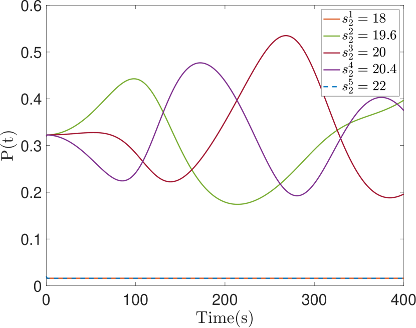
(a) Probability of states

(b) States reached

Figure 1: The probability of Markov states and the states the system reached

5.2 Simulation results

The open-loop behavior of the system with stochastic parameters is shown in Fig. 2(a),2(b). The density and velocity of the mixed-autonomy traffic without control oscillate throughout the whole process. The closed-loop behavior of our stochastic system is shown in Fig. 3(a),3(b). The traffic states deviate from the original states due to the stochastic driving strategy of AVs. The nominal system of HVs and AVs reach their equilibrium points at a finite time with the proposed backstepping control law. We also provide a comparison of the nominal system and stochastic system for open-loop and closed-loop conditions. The error for open-loop results between the nominal and stochastic systems are shown in Fig. 4(a),4(b). The error for closed-loop results between the nominal system and stochastic system are shown in Fig. 5(a),5(b). It is observed that small deviations of density and velocity from the equilibrium still exist after the finite time stabilization is achieved. The maximum density and velocity error for open-loop HVs are $60\text{veh/km}$,$20\text{km/h}$ while the maximum density and velocity error of AVs are $10\text{veh/km}$ and $18\text{km/h}$. The maximum density and velocity error for the close-loop of AVs is $22\text{veh/km}$, $15\text{km/h}$. For HVs, the maximum density and velocity error are $10\text{veh/km}$, $10\text{km/h}$.

In congested mixed-autonomy traffic conditions where AVs employ a more conservative spacing strategy in comparison to HVs, the impact areas of AVs are larger than HVs. The proposed control strategy can ensure the traffic system is in stable condition if the driving strategy of AVs remains relatively consistent with their nominal driving strategy. In the presence of larger gaps between AVs, HVs tend to exhibit gap-filling behavior, colloquially referred to as the “creeping effect”, wherein HVs surpass AVs within such congested regimes.

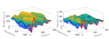
(a) HVs

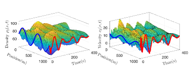
(b) AVs

Figure 2: The open-loop results of the stochastic system

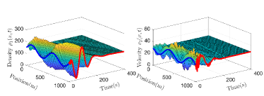
(a) HVs

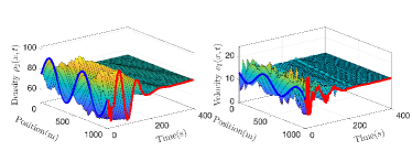
(b) AVs

Figure 3: The close-loop results of the stochastic system

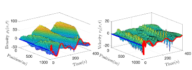
(a) HVs

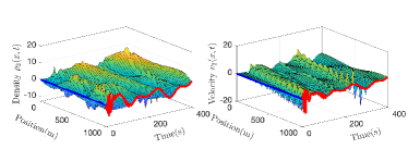
(b) AVs

Figure 4: The density and velocity error between open-loop stochastic system and nominal system

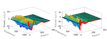
(a) HVs

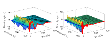
(b) AVs

Figure 5: The density and velocity error between closed-loop stochastic system and nominal system

6 Conclusion

In this paper, a mixed-autonomy traffic PDE model with Markov jumping parameters, is developed to characterize the evolution of traffic density and velocity on the road. The spacing of AVs is considered as a Markov process, rendering the system stochastic in nature. The exponential stability of the nominal system is demonstrated through the employment of a full-state feedback control law using the backstepping method. Subsequently, Lyapunov analysis is utilized to prove the mean-square exponential stability of the stochastic system under the nominal control law. Finally, a numerical simulation is conducted to assess the performance of the control approach for the stochastic system. It is of the author’s future interest to develop control laws that are bale to address other uncertainty of the mixed traffic such as the stochastic arrival rate of AVs and heterogeneous driving behaviors of HVs in response to AVs.

References

- [1] M. Albaba, Y. Yildiz, N. Li, I. Kolmanovsky, and A. Girard. Stochastic driver modeling and validation with traffic data. In 2019 American Control Conference (ACC), pages 4198–4203. IEEE, 2019.
- [2] S. Amin, F. M. Hante, and A. M. Bayen. Exponential stability of switched linear hyperbolic initial-boundary value problems. IEEE Transactions on Automatic Control, 57(2):291–301, 2011.
- [3] H. Anfinsen and O. M. Aamo. Adaptive control of linear2 2 hyperbolic systems. Automatica, 87:69–82, 2018.
- [4] J. Auriol and F. Di Meglio. Minimum time control of heterodirectional linear coupled hyperbolic pdes. Automatica, 71:300–307, 2016.
- [5] J. Auriol and F. Di Meglio. Robust output feedback stabilization for two heterodirectional linear coupled hyperbolic pdes. Automatica, 115:108896, 2020.
- [6] J. Auriol, M. Pereira, and B. Kulcsar. Mean-square exponential stabilization of coupled hyperbolic systems with random parameters. IFAC-PapersOnLine, pages 8823–8828, 2023.
- [7] A. Aw and M. Rascle. Resurrection of” second order” models of traffic flow. SIAM journal on applied mathematics, 60(3):916–938, 2000.
- [8] G. Bastin and J.-M. Coron. Stability and boundary stabilization of 1-d hyperbolic systems, volume 88. Springer, 2016.
- [9] N. Bekiaris-Liberis and A. I. Delis. Pde-based feedback control of freeway traffic flow via time-gap manipulation of acc-equipped vehicles. IEEE Transactions on Control Systems Technology, 29(1):461–469, 2020.
- [10] P. Bolzern, P. Colaneri, and G. De Nicolao. On almost sure stability of continuous-time markov jump linear systems. Automatica, 42(6):983–988, 2006.
- [11] M. Burkhardt, H. Yu, and M. Krstic. Stop-and-go suppression in two-class congested traffic. Automatica, 125:109381, 2021.
- [12] S. Calvert, W. Schakel, and J. Van Lint. Will automated vehicles negatively impact traffic flow? Journal of advanced transportation, 2017, 2017.
- [13] O. L. do Valle Costa, M. D. Fragoso, and M. G. Todorov. Continuous-time Markov jump linear systems. Springer Science & Business Media, 2012.
- [14] E. B. Dynkin. Theory of Markov processes. Courier Corporation, 2012.
- [15] A. Hoyland and M. Rausand. System reliability theory: models and statistical methods. John Wiley & Sons, 2009.
- [16] L. Hu, F. Di Meglio, R. Vazquez, and M. Krstic. Control of homodirectional and general heterodirectional linear coupled hyperbolic pdes. IEEE Transactions on Automatic Control, 61(11):3301–3314, 2015.
- [17] L. Jin, M. Čičić, K. H. Johansson, and S. Amin. Analysis and design of vehicle platooning operations on mixed-traffic highways. IEEE Transactions on Automatic Control, 66(10):4715–4730, 2020.
- [18] A. Kesting, M. Treiber, M. Schönhof, and D. Helbing. Adaptive cruise control design for active congestion avoidance. Transportation Research Part C: Emerging Technologies, 16(6):668–683, 2008.
- [19] I. Kolmanovsky and T. L. Maizenberg. Mean-square stability of nonlinear systems with time-varying, random delay. Stochastic analysis and Applications, 19(2):279–293, 2001.
- [20] M. Krstic and A. Smyshlyaev. Boundary control of PDEs: A course on backstepping designs. SIAM, 2008.
- [21] P.-O. Lamare, J. Auriol, F. Di Meglio, and U. J. F. Aarsnes. Robust output regulation of hyperbolic systems: Control law and input-to-state stability. In 2018 Annual American Control Conference (ACC), pages 1732–1739. IEEE, 2018.
- [22] P.-O. Lamare, A. Girard, and C. Prieur. Switching rules for stabilization of linear systems of conservation laws. SIAM Journal on Control and Optimization, 53(3):1599–1624, 2015.
- [23] X. Li. Trade-off between safety, mobility and stability in automated vehicle following control: An analytical method. Transportation research part B: methodological, 166:1–18, 2022.
- [24] M. J. Lighthill and G. B. Whitham. On kinematic waves ii. a theory of traffic flow on long crowded roads. Proceedings of the Royal Society of London. Series A. Mathematical and Physical Sciences, 229(1178):317–345, 1955.
- [25] V. Milanés and S. E. Shladover. Modeling cooperative and autonomous adaptive cruise control dynamic responses using experimental data. Transportation Research Part C: Emerging Technologies, 48:285–300, 2014.
- [26] R. Mohan and G. Ramadurai. Heterogeneous traffic flow modelling using second-order macroscopic continuum model. Physics Letters A, 381(3):115–123, 2017.
- [27] M. F. Ozkan, A. J. Rocque, and Y. Ma. Inverse reinforcement learning based stochastic driver behavior learning. IFAC-PapersOnLine, 54(20):882–888, 2021.
- [28] C. Prieur, A. Girard, and E. Witrant. Stability of switched linear hyperbolic systems by lyapunov techniques. IEEE Transactions on Automatic control, 59(8):2196–2202, 2014.
- [29] J. Qi, S. Mo, and M. Krstic. Delay-compensated distributed pde control of traffic with connected/automated vehicles. IEEE Transactions on Automatic Control, 2022.
- [30] M. Rausand and A. Hoyland. System reliability theory: models, statistical methods, and applications, volume 396. John Wiley & Sons, 2003.
- [31] P. I. Richards. Shock waves on the highway. Operations research, 4(1):42–51, 1956.
- [32] S. M. Ross. Introduction to probability models. Academic press, 2014.
- [33] R. Vazquez, M. Krstic, and J.-M. Coron. Backstepping boundary stabilization and state estimation of a 2 2 linear hyperbolic system. In 2011 50th IEEE conference on decision and control and european control conference, pages 4937–4942. IEEE, 2011.
- [34] J.-W. Wang, H.-N. Wu, and H.-X. Li. Stochastically exponential stability and stabilization of uncertain linear hyperbolic pde systems with markov jumping parameters. Automatica, 48(3):569–576, 2012.
- [35] K. Yoshida. Lectures on differential and integral equations, volume 10. Interscience Publishers, 1960.
- [36] H. Yu, S. Amin, and M. Krstic. Stability analysis of mixed-autonomy traffic with cav platoons using two-class aw-rascle model. In 2020 59th IEEE Conference on Decision and Control (CDC), pages 5659–5664. IEEE, 2020.
- [37] H. Yu and M. Krstic. Traffic congestion control for aw–rascle–zhang model. Automatica, 100:38–51, 2019.
- [38] H. Yu and M. Krstic. Traffic Congestion Control by PDE Backstepping. Springer, 2022.
- [39] H. M. Zhang. A non-equilibrium traffic model devoid of gas-like behavior. Transportation Research Part B: Methodological, 36(3):275–290, 2002.
- [40] L. Zhang and C. Prieur. Stochastic stability of markov jump hyperbolic systems with application to traffic flow control. Automatica, 86:29–37, 2017.
- [41] L. Zhang, C. Prieur, and J. Qiao. Pi boundary control of linear hyperbolic balance laws with stabilization of arz traffic flow models. Systems & Control Letters, 123:85–91, 2019.
- [42] P. Zhang, R.-X. Liu, S. Wong, and S.-Q. Dai. Hyperbolicity and kinematic waves of a class of multi-population partial differential equations. European Journal of Applied Mathematics, 17(2):171–200, 2006.