Generative and Contrastive Paradigms Are Complementary for
Graph Self-Supervised Learning

Abstract.

For graph self-supervised learning (GSSL), masked autoencoder (MAE) follows the generative paradigm and learns to reconstruct masked graph edges or node features. Contrastive Learning (CL) maximizes the similarity between augmented views of the same graph and is widely used for GSSL. However, MAE and CL are considered separately in existing works for GSSL. We observe that the MAE and CL paradigms are complementary and propose the graph contrastive masked autoencoder (GCMAE) framework to unify them. Specifically, by focusing on local edges or node features, MAE cannot capture global information of the graph and is sensitive to particular edges and features. On the contrary, CL excels in extracting global information because it considers the relation between graphs. As such, we equip GCMAE  with an MAE branch and a CL branch, and the two branches share a common encoder, which allows the MAE branch to exploit the global information extracted by the CL branch. To force GCMAE  to capture global graph structures, we train it to reconstruct the entire adjacency matrix instead of only the masked edges as in existing works. Moreover, a discrimination loss is proposed for feature reconstruction, which improves the disparity between node embeddings rather than reducing the reconstruction error to tackle the feature smoothing problem of MAE. We evaluate GCMAE  on four popular graph tasks (i.e., node classification, node clustering, link prediction, and graph classification) and compare it with 14 state-of-the-art baselines. The results show that GCMAE  consistently provides good accuracy across these tasks, and the maximum accuracy improvement is up to 3.2% compared with the best-performing baseline.

1. Introduction

Graphs model entities as nodes and the relations among the entities as edges and prevail in many domains such as social networks (Hamilton et al., 2017; Veličković et al., 2017), finance (Liu et al., 2021), biology (Dai et al., 2018), and medicine (Liu et al., 2020). By conducting message passing on the edges and utilizing neural networks to aggregate messages on the nodes, graph neural network (GNN) models perform well for various graph tasks, e.g., node classification, node clustering, link prediction, and graph classification (Guo and Dai, 2022; Zhu et al., 2021; Hamilton et al., 2017; Zhang et al., 2020; Zheng et al., 2022). These tasks facilitate many important applications including recommendation, fraud detection, community detection, and pharmacy (Lu et al., 2022; Gao et al., 2021a; Cui et al., 2021; Chen et al., 2023a, b). To train GNN models, graph self-supervised learning (GSSL) is becoming increasingly popular because it does not require label information (You et al., 2020; Yin et al., 2022), which can be rare or expensive to obtain in practice. Existing works handle GSSL with two main paradigms (Wu et al., 2021; Li et al., 2023b), i.e., masked autoencoder (MAE) and contrastive learning (CL).

Graph MAE methods usually come with an encoder and a decoder, which are both GNN models (Hou et al., 2022; Hou et al., 2023; Li et al., 2022b; Li et al., 2023b; Tan et al., 2023). The encoder computes node embeddings from a corrupted view of the graph, where some of the edges or node features are masked; the decoder is trained to reconstruct the masked edges or node features using these node embeddings. Graph MAE methods achieve high accuracy for graph tasks but we observe that they still have two limitations. ❶ Graph MAE misses global information of the graph, which results in sub-optimal performance for tasks that require a view of the entire graph (e.g., graph classification) (Chien et al., 2021; Wei et al., 2022). This is because both the encoder and decoder GNN models use a small number of layers (e.g., 2 or 3), and a k-layer GNN can only consider the k-hop neighbors of each node (Chen et al., 2020b). Thus, both the encoder and decoder consider the local neighborhood. ❷ Graph MAE is prone to feature smoothing, which means that neighboring nodes tend to have similar reconstructed features and harms performance for tasks that rely on node features (e.g., node classification). This is because the encoder and decoder GNN models aggregate the neighbors to compute the embedding for each node, and due to this local aggregation, GNN models are widely known to suffer from the over-smoothing problem (Zhao and Akoglu, 2019; Chen et al., 2020b), which also explains why GNN cannot use many layers.

Graph CL methods usually generate multiple perturbed views of a graph via data augmentation and train the model to maximize the similarity between positive pairs (e.g., an anchor node and its corresponding node in another view) and minimize the similarity between negative pairs (e.g., all other nodes except the positive pairs) (Li et al., 2022a; Cai et al., 2023). As graph CL can contrast nodes that are far apart (e.g., ¿ 3 hops) in multiple views, it captures global information of the entire graph. However, without reconstruction loss for the node features and edges, CL is inferior to MAE in learning local information for the nodes or edges, and thus may have sub-optimal performance for tasks that require such information (e.g., link prediction and clustering) (You et al., 2020, 2021).

The above analysis shows that graph MAE and CL methods potentially complement each other in capturing local and global information of the graph. Thus, combining MAE and CL may yield better performance than using them individually. Figure 1 shows such an example with node clustering. As a representative graph CL method, CCA-SSG (Zhang et al., 2021b) has poor clustering for the nodes due to the lack of the local information. For GraphMAE (Hou et al., 2022), a state-of-the-art graph MAE method, the node clusters are more noticeable by capturing local information. However, by combining MAE and CL, our GCMAE  yields the best node clustering and hence the highest accuracy among the three methods. Although the idea sounds straightforward, a framework that combines MAE and CL needs to tackle two key technical challenges. ❶ MAE and CL have different graph augmentation logic and learning objectives (i.e., reconstruction and discrimination), and thus a unified view is required to combine them. ❷ MAE and CL focus on local and global information respectively, so the model architecture should ensure that the two kinds of information complement each to reap the benefits.

Table 1. Performance improvements of our GCMAE over the best-performing baselines in each category for different tasks. Others are specialized methods for each task.

Graph Task	vs. Contrastive	vs. MAE	Others
Node classification	4.8%	2.2%	12.0%
Link prediction	4.4%	1.5%	-
Node clustering	8.8%	3.2%	14.7%
Graph classification	2.5%	4.2%	-

To tackle these challenges, we design the graph contrastive masked autoencoder (i.e., GCMAE ) framework. We first show that MAE and CL can be unified in one mathematical framework despite their apparent differences. In particular, we express MAE as a special kind of CL, which uses masking for data augmentation and maximizes the similarity between the original and masked graphs. This analysis inspires us to use an MAE branch and a CL branch in GCMAE  and share the encoder for the two branches. The MAE branch is trained to reconstruct the original graph while the CL branch is trained to contrast two augmented views; and the shared encoder is responsible for mapping the graphs (both original and augmented) to the embedding spaces to serve as inputs for the two branches. By design, the shared encoder conducts input mapping and transfers information between both branches. As such, local information and global information are condensed in the shared encoder and benefit both MAE and CL. Furthermore, to tackle the feature smoothing problem of MAE that makes the reconstructed features of neighboring nodes similar, we introduce a discrimination loss for model training, which enlarges the variance of the node embeddings to avoid smoothing. Instead of training MAE to reconstruct only the masked edges as in existing works, we reconstruct the entire adjacency matrix such that MAE can learn to capture global information of the graph structures.

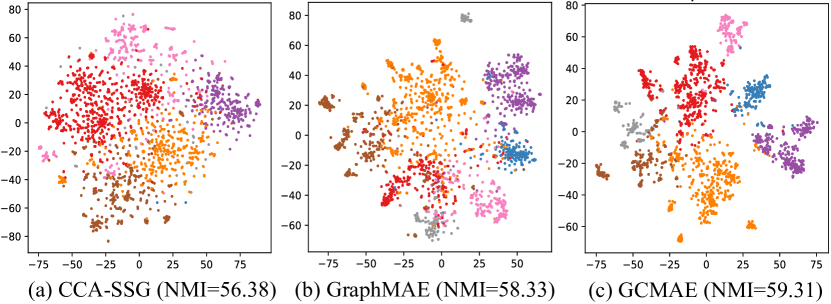
Figure 1. We conduct node clustering on the Cora and visualize the node embeddings learned by our GCMAE, GraphMAE, and CCA-SSG with t-SNE. GraphMAE and CCA-SSG represent MAE and CL methods, respectively. Nodes of the same category are plotted in the same color. We use Normalized Mutual Information (NMI) to evaluate the clustering effect, with a larger value indicating better accuracy.

We evaluate our GCMAE on four popular graph tasks, i.e., node classification, node clustering, link prediction, and graph classification. These tasks have essentially different properties and require different information in the graph. We compare GCMAE  with state-of-the-art baselines, including graph MAE methods such as GraphMAE (Hou et al., 2022), SeeGera (Li et al., 2023b), S2GAE (Tan et al., 2023), and MaskGAE (Li et al., 2022b), and graph CL methods such as GDI (Veličković et al., 2017), MVGRL (Hassani and Khasahmadi, 2020), GRACE (Zhu et al., 2020), and CCA-SSG (Zhang et al., 2021b). The results show that GCMAE yields consistently good performance on the four graph tasks and is the most accurate method in almost all cases (i.e., a case means a dataset plus a task). As shown in Table 1, GCMAE outperforms both contrastive and MAE methods, and the improvements over the best-performing baselines are significant. We also conduct an ablation study for our model designs (e.g., shared encoder and the loss terms), and the results suggest that the designs are effective in improving accuracy.

To summarize, we make the following contributions:

• We observe the limitations of existing graph MAE and CL methods for graph self-supervised learning (GSSL) and propose to combine MAE and CL for enhanced performance.

• We design the GCMAE framework, which is the first to jointly utilize MAE and CL for GSSL to our knowledge.

• We equip GCMAE  with tailored model designs, e.g., the shared encoder for information sharing between MAE and CL, the discrimination loss to combat feature smoothing, and training supervision with adjacency matrix reconstruction.

• We conduct extensive experiments to evaluate GCMAE  and compare it with state-of-the-art, demonstrating that GCMAE  is general across graph tasks and effective in accuracy.

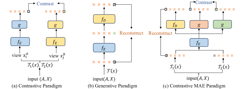
Figure 2. Architectures of the generative paradigm, contrastive paradigm, and our GCMAE  for graph self-supervised learning. Contrast means the contrastive loss while Reconstruct means the reconstruction loss.

2. PRELIMINARIES

In this part, we introduce the basics of MAE and CL for GSSL to facilitate our formulation. The discussions on specific MAE and CL methods are provided in Section 6. We use $G=(\bm{V},\bm{E})$ to denote a graph, where $\bm{V}=\{v_{1},v_{2},\cdot\cdot\cdot,v_{N}\}$ is the set of nodes with $|\bm{V}|=N$ and $\bm{E}$ is the set of edges. The adjacency matrix of the graph is $\bm{A}\in\{0,1\}^{N\times N}$, and the node feature matrix is $\bm{X}\in\mathbb{R}^{N\times d}$, where $x_{i}\in\mathbb{R}^{d}$ is the feature vector of $v_{i}$ with dimension $d$ and $\bm{A}_{ij}=1$ if edge $(v_{i},v_{j})\in\bm{E}$.

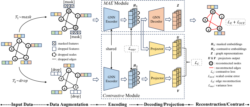
Figure 3. Structure of our GCMAE  framework, which consists of an MAE branch and a contrastive branch with a shared encoder.

2.1. Contrastive Learning (CL) for GSSL

CL has been very popular for GSSL due to its good performance for various application scenarios, such as social network analysis (Zhang et al., 2021b), molecular detection (Ma et al., 2021), and financial deception (Sahu et al., 2020). Generally, graph CL follows a “augmenting-contrasting” pattern, where the graph views are corrupted via the data augmentation strategies $\mathcal{T}_{1}$ and $\mathcal{T}_{2}$ (e.g., node feature masking and node dropping), and then a GNN encoder $f_{\theta}$ is used to encode the corrupted views into node embeddings. The goal of CL is to maximize the mutual information between the two corrupted views, which is achieved by maximizing the similarity of node embeddings as a surrogate. Thus, CL does not require label information and conducts learning by distinguishing between node embeddings in different views. Figure 2 (a) shows the framework of graph contrastive learning. The objective of CL is essentially to maximize the similarity function between two node embeddings encoded through a GNN encoder $f_{\theta}$, which can be formulated as:

(1) $$\max_{\theta}\mathop{\mathbb{E}}\limits_{x\sim\mathcal{D}}S\left(f_{\theta}\left(\mathcal{T}_{1}\left(\bm{A},\bm{X}\right)\right),f_{\theta}\left(\mathcal{T}_{2}\left(\bm{A},\bm{X}\right)\right)\right),$$

where $\theta$ represents the network weights, node feature vector $x$ follows the input data distribution $\mathcal{D}$, and $S\left(\cdot,\cdot\right)$ is the similarity function to measure the similarity between node embeddings.

2.2. Masked Autoencoder (MAE) for GSSL

Different from graph CL methods, graph MAE follows a “masking-reconstructing” pattern. The overview of graph MAE methods is shown in Figure 2 (b). In general, graph MAE methods first randomly mask node features or edges with mask patches $\bm{M}$, where $x\odot\bm{M}$ represents visible tokens and $x\odot(1-\bm{M})$ means masked tokens. Graph MAE leverages the encoder $f_{\theta}$ to encode the visible tokens into node embeddings, and then the decoder $d_{\phi}$ attempts to reconstruct the masked tokens by decoding from the node embeddings. Thus, we wish to maximize the similarity between the masked tokens and the reconstructed tokens:

(2) $$\max_{\theta,\phi}\mathop{\mathbb{E}}\limits_{x\sim\mathcal{D}}S\left(d_{\phi}\left(h\right)\odot(1-\bm{M}),x\odot(1-\bm{M})\right),h=f_{\theta}\left(x\odot\bm{M}\right),$$

where $\odot$ means element-wise product, $h$ is the node embedding learned by the encoder, and $S\left(\cdot,\cdot\right)$ is the similarity function for MAE modeling.

3. The GCMAE Framework

Since graph MAE cannot benefit from global information, it can only learn from limited neighbor nodes, which may eventually lead to similar graph representations. We are inspired by the successful application of CL, where global information can be learned by contrasting the anchor node with distant nodes. The overall framework is shown in Figure 3.

3.1. Unifying CL and MAE for GSSL

Even though contrastive and generative approaches have achieved individual success, there is a lack of systematic analysis regarding their correlation and compatibility in one single framework. Motivated as such, we aim to explore a unified Contrastive MAE paradigm to combine contrastive paradigm and MAE paradigm. From Equation 2, we can conclude that graph MAE essentially maximizes the similarity between node embeddings reconstructed via decoder and the masked tokens, which is formally analogous to Equation 1. In other words, both the contrastive paradigm and the generative paradigm are maximizing the similarity between two elements within the function.

Let us still focus on Equation 2, graph MAE wishes to find a theoretically optimal decoder that can reconstruct the masked tokens losslessly. Suppose we can achieve the decoder $d{}^{\prime}_{\phi{}^{\prime}}$ parameterized by $\phi{}^{\prime}$ that satisfies $d{}^{\prime}_{\phi{}^{\prime}}\left(f_{\theta}\left(x\odot(1-\bm{M})\right)\right)\cdot(1-\bm{M})\approx x\odot\left(1-\bm{M}\right)$ as closely as possible. Then, we transform Equation 2 into the following form:

(3) $$\max_{\theta,\phi,\phi^{{}^{\prime}}}S(d_{\phi}(h)\odot(1\!-\!\bm{M})\!-\!d{}^{\prime}_{\phi{}^{\prime}}(h)\odot(1-\bm{M})),$$

where $\phi^{\prime}$ is optimized in the following form:

(4) $$\phi{}^{\prime}\!=\!{\mathrm{arg}\max_{\phi{}^{\prime}}}\mathop{\mathbb{E}}\limits_{x{}^{\prime}\sim\mathcal{D}}S(d{}^{\prime}_{\phi{}^{\prime}}(f_{\theta}(x{}^{\prime}\!\odot\!(1\!-\!\bm{M})))\!\odot\!(1\!-\!\bm{M})\!-\!x{}^{\prime}\!\odot\!(1\!-\!\bm{M})),$$

where $x{}^{\prime}$ is the feature token reconstructed by the optimal decoder $d{}^{\prime}_{\phi{}^{\prime}}$. Notice that since $d$ and $d{}^{\prime}$ have the same architecture, we let $d=d{}^{\prime}$. Inspired by (Kong and Zhang, 2023), we further simplify Equation 3, and define the loss function for MAE:

(5) $$\mathcal{L}(h_{1},h_{2},\phi,\phi{}^{\prime})=\max_{\phi,\phi^{{}^{\prime}}}S(d_{\phi}(h_{1}),d_{\phi{}^{\prime}}(h_{2}))\odot(1-\bm{M}),$$

where $h_{1},h_{2}$ are the hidden embeddings derived from two augmentation strategies:

(6) $$\begin{cases}&h_{1}=f_{\theta}(\mathcal{T}_{1}(x))=f_{\theta}(x\odot\bm{M}),\\ &h_{2}=f_{\theta}(\mathcal{T}_{2}(x))=f_{\theta}(x\odot(1-\bm{M})).\end{cases}$$

In this way, we rewrite the generative paradigm into a form similar to the contrastive paradigm, both with data augmentation and optimizing a similarity function.

In order to integrate MAE and CL into one optimization framework, a novel self-supervised paradigm, Contrastive MAE paradigm. The MAE branch is trained to reconstruct the masked tokens using similarity function $S_{1}$ while the CL branch is trained to contrast two augmented views using similarity function $S_{2}$:

(7) $$\mathcal{L}(x,\bm{M},h_{1},h_{2},\theta,\phi)\!=\!\max_{\theta,\phi}S_{1}(d_{\phi}(h_{1}),x\!\odot\!(1\!-\!\bm{M}))\!+\!S_{2}(h_{1},h_{2}).$$

Summary. Despite the recent attempts by contrastive MAE methods (Qi et al., 2023; Huang et al., 2022), understanding their underlying rationale remains an open question. Therefore, we provide a theoretical analysis showing that the nature of the generative paradigm is essentially similar to that of CL. Rather than treating them separately, these two paradigms can potentially complement each other, compensating for their respective shortcomings and obtaining better performance. Moreover, both the generative and contrastive paradigms share similar optimization objectives, which enables us to optimize them within a unified framework.

3.2. Structure of the GCMAE Framework

Objective: In this paper, we aim to unify graph MAE and CL into a single framework and further reveal the intrinsic relation between graph MAE and CL, where CL can help graph MAE to achieve global information, through which we hope to further improve the performance of graph MAE on various downstream tasks.

Overview: We propose a novel graph SSL framework to incorporate CL into graph MAE. Overall, our framework consists of two core modules: the MAE Module and the Contrastive Module, which are used to reconstruct masked nodes and contrast two corrupted views, respectively. To achieve our design goal, we introduce three main components:

• Shared encoder. We take the masked graph in Graph MAE as an augmented view, and then generate another view by randomly dropping nodes. We leverage a shared encoder to connect both modules and encode the corrupted views into hidden node embeddings. In this way, the contrastive module can transfer the global information to the MAE module. The node embedding generated from MAE module is used to calculate feature reconstruction loss using Scaled Cosine Error (SCE) $\mathcal{L}_{SCE}$, and another node embedding is leveraged to compute contrastive loss $\mathcal{L}_{C}$.

• Discrimination loss. Low discriminative input node features will cause graph MAE to generate similar node representations. Thus, we propose a novel discrimination loss $\mathcal{L}_{Var}$, which improves feature discriminability by increasing the variance between node hidden embeddings (i.e., the output of the shared encoder).

• Adjacency matrix reconstruction. In order to further improve performance on link prediction and node clustering, we reconstruct the entire graph and calculate the adjacency matrix reconstruction error $\mathcal{L}_{E}$. This is because reconstructing the limited masked edges is not enough to learn the entire graph structures.

Therefore, the overall loss function for GCMAE is defined as follows:

(8) $$\mathcal{J}=\mathcal{L}_{SCE}+\alpha\mathcal{L}_{C}+\lambda\mathcal{L}_{E}+\mu\mathcal{L}_{Var},$$

where $\alpha,\lambda$ and $\mu$ are hyper-parameter used to adjust the weights. In summary, the contrastive module learns global information by contrasting two corrupted views and transfers it to the MAE module with a shared encoder. Before decoding, discrimination loss is leveraged to improve the discrimination between node embeddings to avoid yielding similar node representations. We reconstruct the node features and adjacency matrix in the MAE module.

4. Model Designs

In this section, we present a detailed description of the proposed GCMAE. We introduce each core component individually with the following three questions in our mind:

• Q1: How to learn global information for graph MAE?

• Q2: How to train a decent encoder to learn the entire graph structures?

• Q3: How to enhance the feature discrimination?

Recently, GraphMAE (Hou et al., 2022) has attracted great attention in graph SSL due to its simple but effective framework. Therefore, we choose GraphMAE as the backbone in this paper. For a node set $\bm{V}$, we randomly select a subset of node $\widetilde{\bm{V}}\subseteq\bm{V}$ and mask their corresponding features $\bm{X}$, i.e., setting its feature values to 0. We sample $\widetilde{\bm{V}}$ following a specific distribution, i.e., Bernoulli distribution. This masking strategy is a common but effective strategy in a wide range of previous applications (You et al., 2020; Thakoor et al., 2021). We consider this node masking operation as a random data augmentation in graph CL methods (Zhu et al., 2021; Sun et al., 2019). Then the node feature $\hat{x_{i}}$ for node $v_{i}\in\widetilde{\bm{V}}$ in the masked feature mask $\hat{\bm{X}}$ can be defined as follow:

(9) $$\hat{x}_{i}=\begin{cases}0,&v_{i}\in\widetilde{\bm{V}}\\ x_{i},&v_{i}\in\bm{V}\end{cases}$$

Further, given an encoder $f_{E}$ and GNN decoder $f_{D}$ define the embedding code:

(10) $$\bm{H_{1}}=f_{E}(\bm{A},\hat{\bm{X}})\quad\bm{Z}=f_{D}(\bm{A},\bm{H_{1}}),$$

where $\bm{H_{1}}\in\mathbb{R}^{N\times d^{h}}$ is the hidden embedding of the feature masking view encoded by $f_{E}$ and then used as the input of GNN decoder $f_{d}$ to obtain the node representations $\bm{Z}\in\mathbb{R}^{N\times d{}^{\prime}}$. $d^{h}$ is the dimension of hidden embedding. Then we calculate the SCE loss:

(11) $$\mathcal{L}_{\mathrm{SCE}}=\frac{1}{|\widetilde{V}|}\sum_{v_{i}\in\widetilde{V}}(1-\frac{x_{i}^{T}h_{i}}{\|x_{i}\|\cdot\|z_{i}\|})^{\gamma},\gamma>1,$$

where $\gamma$ is leveraged to adjust the hyperparameter of loss convergence speed, $h_{i}$ is the hidden embedding vector of node $v_{i}$, and $z_{i}$ is the node representation of node $v_{i}$.

4.1. Shared Encoder

We reveal the intrinsic correlation between CL and Graph MAE and mathematically analyze the feasibility of jointly optimizing them in Section 3.1. However, how to efficiently transfer global information without complicated structural design is still an unsolved problem. Therefore, we ask here:

how to transfer global information from the contrastive module to the MAE module?

An intuitive solution is to train two encoders to encode the CL branch and the MAE branch separately, and then fuse the learned node embeddings. However, this inevitably faces two issues: ❶ training two codes independently cannot realize information transfer between branches. ❷ the strategy of fusion embedding will introduce an unnecessary design burden. Moreover, the accuracy performance depends on the lower bound of either embedding, and low-quality node embeddings will directly affect the performance.

To tackle the problem, we introduce a shared encoder that simultaneously encodes two augmented views to learn local and global information. The contrastive module leverages the shared encoder to transfer the global information from the entire graph to assist Graph MAE in learning meaningful representations and fine-tuning local network parameters. We do not need an additional embedding fusion strategy, since the shared encoder can directly yield the unify node embeddings. Thus, we first use the shared encoder $f_{E}$ to encode the corrupted graph $\bar{\bm{A}}$ augmented by random node dropping into hidden embeddings:

(12) $$\bm{H_{2}}=f_{E}(\bar{\bm{A}},\bm{X}),$$

where $\bm{H_{2}}\in\mathbb{R}^{N\times d^{h}}$. Then, we utilize two projectors $g_{1}$, $g_{2}$ to map $\bm{H_{1}}$ ,$\bm{H_{2}}$ into different vector spaces:

(13) $$\bm{U}=\sigma(g_{1}(\bm{H_{1}},\psi_{1})),\quad\bm{V}=\sigma(g_{2}(\bm{H_{2}},\psi_{2})),$$

where $\sigma(\cdot)$ is a nonlinear activation function. The projector consists of a simple two-layer perceptron model with bias $\psi_{1},\psi_{2}$. We use the classical InfoNCE as the contrastive loss function, defined for each positive sample pair $(u_{i},v_{i})$ as:

(14) $$\ell_{c}=-\log{\frac{\exp(s(u_{i}^{a},v_{i}^{b})/\tau)}{\sum_{j=1}^{n}[\exp(s(u_{i}^{a},v_{j}^{a}))/\tau+\exp(s(u_{i}^{a},v_{j}^{b})/\tau)]}},$$

where $\tau$ is the temperature parameter and $s(\cdot)$ is the cosine similarity between $u_{i}$ and $v_{i}$, while $u_{i}^{a}\in\bm{U}$ and $u_{j}^{b}\in\bm{V}$ denote the projected vector of $v_{i}$ and $v_{j}$, respectively. Since the two projectors are symmetric, the loss for the node pair $(v_{i},u_{i})$ is defined similarly. The overall objective of the contrastive module is to maximize the average mutual information of all positive sample pairs in the two views. Formally, it is defined as:

(15) $$\mathcal{L}_{C}=\frac{1}{2N}\sum_{i=1}^{N}[\ell_{c}(u_{i},v_{i})+\ell_{c}(v_{i},u_{i})].$$

4.2. Adjacency Matrix Reconstruction

Graph data exhibits a unique property of complex topology when compared to images and text, as graph contains complex graph topology and node features. Several studies have focused on adjacency matrix reconstruction (Hu et al., 2019; Hu et al., 2020). Since it not only helps models pay more attention to link relationships but also facilitates the encoder to get rid of the constraints brought by fitting extreme feature values (Jin et al., 2020). By incorporating the adjacency matrix, the overall objective lightens the weight of feature reconstruction, thereby eliminating the incomplete learned knowledge caused by a single objective. Different from MaskGAE (Li et al., 2022b) reconstructing limited edges, we reconstruct node features and adjacency matrices at the same time, which can help the model capture the global graph structures rather than particular edges or paths. In this work, we employ the output representation of the decoder to directly reconstruct the adjacency matrix:

(16) $$\ell_{MSE}=\frac{1}{N^{2}}\sum_{i,j}(\hat{\bm{A}}_{ij}-\bm{A}_{ij})^{2},\quad\hat{\bm{A}}=\left\langle\bm{Z},\bm{Z}^{T}\right\rangle=\bm{Z}\bm{Z}^{T},$$

where $\hat{\bm{A}}_{ij}$ is the probability of an edge existing between nodes $v_{i}$ and $v_{j}$. The MSE function measures the distance between the reconstructed adjacency matrix and the original adjacency matrix, ensuring consistency between the latent embedding and the input graph structure. However, due to the discretization and sparsity of the adjacency matrix, solely using MSE would make the model overfit to zero values. Therefore, we adopt Cross-Entropy (CE) to determine the existence of an edge between two nodes:

(17) $$\ell_{BCE}=-\frac{1}{N^{2}}\sum_{i,j}[\bm{A}_{ij}\cdot\log\hat{\bm{A}}_{ij}+(1-\bm{A}_{ij})\cdot\log(1-\hat{\bm{A}}_{ij})].$$

In addition to the above issues, graph data is low-density and the degree distribution follows a power-law distribution, which cannot be adequately estimated by simple MSE and CE. The coexistence of both low-degree and high-degree nodes further renders Euclidean spaces invalid and hampers the training speed. To address this problem, we put forth the Relative Distance (RD) loss function:

(18) $$\ell_{DIST}=-\log\frac{{\sum_{{(i,j)\in\bm{E}}}}D(z_{i},z_{j})}{{\textstyle\sum_{(i,j)\notin\bm{E}}}D(z_{i},z_{j})},$$

where $D(\cdot,\cdot)$ defines the distance between node $v_{i}$ and node $v_{j}$, and $z$ is the node representation of the decoder in the MAE module. The numerator and denominator in the RD loss function correspond to the sum of distances between adjacent nodes and non-adjacent nodes, respectively. Reconstructing the original degree distribution is an NP-hard problem. Inspired by CL, we are no longer obsessed with learning the original target distribution, but shift to a proxy task of evaluating node similarity. The final adjacency matrix reconstruction error is a combination of the three loss functions mentioned above:

(19) $$\mathcal{L}_{E}=\ell_{MSE}+\ell_{BCE}+\ell_{DIST}.$$

4.3. Discrimination Loss

Graph MAE approaches have achieved good classification performance, however, the presence of difficult-to-distinguish dimensions in the features can easily lead to deteriorated training. In comparison to the sparsity and discretization characteristics of graph data, pixel and text feature vectors possess a higher information density and more significant discrimination between each other. The low discrimination in graph data is primarily due to node features being vector representations of text, which are compressed representations of keywords obtained through feature extractors.

Previous research has demonstrated a strong correlation between feature discrimination and the performance of Graph MAE (Hou et al., 2023). Graph MAE may mislead the model and facilitate the propagation of harmful substances when reconstructing node features, as numerous information may be related to erroneous evaluations. In other words, graph MAE attempts to reconstruct the cancerous node features, which results in model collapse and drives the learned representations to be similar. This observation further inspires us to design a novel loss function to narrow down the gap between Graph MAE and feature discrimination.

To address the above challenges, we introduce a variance-based discrimination loss, which aims to assist the encoder in learning discriminative embeddings and cushion the impact caused by erroneous information to the network. More importantly, this variance term enforces different node representations within the same embedding matrix are diverse, compensating for the lack of original feature discrimination. The regularized standard deviation is defined as follows:

(20) $$\mathcal{L}_{Var}(h,\epsilon)=\sqrt{\mathrm{Var}(h)+\epsilon},$$

where $\epsilon$ is a small scalar to prevent numerical instability when reducing to 0 values. $\mathrm{Var}(h)$ is the variance of hidden embeddings (i.e., the output of the shared encoder). This regularization encourages the encoder to map inputs to a different space within a specific range of variances, thereby preventing the model from collapsing to the same vector.

Algorithm 1 The training procedure of GCMAE

1:Graph $G=(\bm{A},\bm{X})$, shared encoder $f_{E}$, decoder $f_{D}$, projectors $g_{1},g_{2}$, feature masking $\mathcal{T}_{1}$, node dropping $\mathcal{T}_{2}$, Epochs $E$

2:Trained GNN encoder $f_{E}$

3:Initialize the GNN encoder $f_{E}$

4:for each $epoch\in E$ do

5:     Generate corrupted views $\mathcal{T}_{1}(G)$, $\mathcal{T}_{2}(G)$

6:     $\bm{H_{1}}=f_{E}(\mathcal{T}_{1}(G))$,  $\bm{H_{2}}=f_{E}(\mathcal{T}_{2}(G))$

7:     Decoding from hidden embedding $\bm{Z}=f_{D}(\bm{A},\bm{H_{1}})$

8:     $\bm{U}=g_{1}(\bm{H_{1}}),\quad\bm{V}=g_{2}(\bm{H_{2}})$

9:     Calculate loss function $\mathcal{J}=\mathcal{L}_{SCE}+\mathcal{L}_{C}+\mathcal{L}_{E}+\mathcal{L}_{Var}$

10:     Update $f_{E}$ with $\mathcal{J}$

11:end for

Algorithm 1 summarizes the overall training process of GCMAE  with all the loss terms.

4.4. Limitations

Although GCMAE  enjoys the advantages of both CL and MAE and thus provides strong performance as we will show in Section 5, it still reveals several limitations. One drawback of GCMAE  is that its training time may be relatively long because it uses two branches for CL and MAE and learns to reconstruct the entire adjacency matrix. As the adjacency matrix contains many edges for large graphs, the time consumption could be high. To alleviate this problem, we sample multiple sub-graphs from the original graph for reconstruction. As we will report in Section 5.4, the training time of GCMAE  is comparable to the baseline methods.

5. Experimental Evaluation

In this part, we extensively evaluate our GCMAE  along with state-of-the-art baselines on 4 graph tasks, i.e., node classification, link prediction, node clustering, and graph classification. We aim to to answer the following research questions:

• RQ1: How does GCMAE  compare with the baselines in terms of the accuracy for the graph tasks?

• RQ2: Does GCMAE  achieve its design goals, i.e., improving MAE with CL?

• RQ3: How efficient it is to train GCMAE ?

• RQ4: How do our designs and the hyper-parameters affect the performance of GCMAE ?

Table 2. Statistics of the datasets used for node classification, link prediction, and node clustering.

Dataset	# Nodes	# Edges	# Features	# Classes
Cora	2,708	10,556	1,433	7
Citeseer	3,327	9,228	3,703	6
PubMed	19,717	88,651	500	3
Reddit	232,965	11,606,919	602	41

5.1. Experiment Settings

Datasets. We conduct the experiments on 10 public graph datasets, which are widely used to evaluate graph self-supervised learning methods (Velickovic et al., 2019; Hou et al., 2022; Zhu et al., 2020). In particular, the 4 citation networks in Table 2 are used for node classification, link prediction, and node clustering, and the 6 graphs in Table 3 are used for graph classification. Note that each dataset in Table 2 is a single large graph while each dataset in Table 3 contains many small graphs for graph classification. We intentionally choose these graphs for diversity, i.e. they have nodes ranging from thousands to millions, with varying classes.

Baselines. We compare GCMAE with 14 state-of-the-art methods on the 4 graph tasks, which span the following 3 categories:

• Supervised methods directly train their models with labeled data, and we choose 2 classical GNN models, i.e., GCN (Kipf and Welling, 2016a) and GAT (Veličković et al., 2017), for node classification.

• Contrastive methods learn to generate the node embeddings by discriminating positive and negative node pairs. Then, the embeddings serve as input for a separate model (e.g., SVM), which is tuned for the downstream task with labeled data. Following GraphMAE (Hou et al., 2022), we use DGI (Velickovic et al., 2019), MVGRL (Hassani and Khasahmadi, 2020), GRACE (Zhu et al., 2020), and CCA-SSG (Zhang et al., 2021b) for node classification, link prediction, and node clustering. For graph classification, we choose 4 graph-level contrastive methods, i.e., Infograph (Sun et al., 2019), GraphCL (You et al., 2020), JOAO (You et al., 2021), and InfoGCL (Xu et al., 2021).

• Masked autoencoder (MAE) methods adopt a “mask-reconstruct” structure to learn the node embeddings, and like the contrastive methods, a separate model is tuned for each downstream task. Following SeeGera (Li et al., 2023b), we use 4 graph MAE models, i.e., GraphMAE (Hou et al., 2022), SeeGera (Li et al., 2023b), S2GAE (Tan et al., 2023), and MaskGAE (Li et al., 2022b) for node classification, link prediction, clustering, and graph classification.

• Deep clustering methods are specially designed for node clustering and design objectives tailored for clustering to guide model training. We include 3 such methods, i.e., GC-VGE (Guo and Dai, 2022), SCGC (Liu et al., 2023), and GCC (Fettal et al., 2022).

Note that some baselines may not apply for a task, e.g., the supervised methods only work for node classification, and thus we apply the baselines for the tasks when appropriate. For the contrastive and MAE methods, we use LIBSVM (Chang and Lin, 2011) to train SVM classifiers for node classification and graph classification following GraphMAE (Hou et al., 2022) and SeeGera (Li et al., 2023b). 5-fold cross-validation is used to evaluate performance for the tasks. For link prediction, we fine-tune the final layer of the model using cross-entropy following MaskGAE (Li et al., 2022b). For node clustering, we apply K-means (Arthur and Vassilvitskii, 2006) on the node embeddings. We use the Adam optimizer with a weight decay of 0.0001 for our method, and set the initial learning rate as 0.001. We conduct training on one NVIDIA GeForce RTX 4090 GPUs with 24GB memory.

Table 3. Statistics of the datasets used for graph classification.

Dataset	# Graphs	# Classes	Avg. # Nodes
IMDB-B	1,000	2	19.8
IMDB-M	1,500	3	13
COLLAB	5,000	3	74.5
MUTAG	188	2	17.9
REDDIT-B	2,000	2	429.7
NCI1	4,110	2	29.8

Performance metrics. We are mainly interested in the accuracy of the methods and use well-established accuracy measures for each task (Hou et al., 2022). In particular, we adopt the Accuracy score (ACC) for node classification, the Area Under the Curve (AUC) and Average Precision (AP) for link prediction, Normalized Mutual Information (NMI) and Adjusted Rand Index (ARI) for node clustering, and Accuracy score (ACC) for graph classification. For all these measures, larger values indicate better performance. For each case (i.e., dataset plus task), we report the average accuracy and standard deviation for each method over 5 runs with different seeds.

Table 4. Node classification accuracy scores for the experimented methods. For each graph, we mark the most accurate method in boldface and the runner-up with underline.

	Method	Cora	Citeseer	PubMed	Reddit
Supervised	GCN	81.48±0.58	70.34±0.62	79.00±0.50	95.30±0.10
	GAT	82.99±0.65	72.51±0.71	79.02±0.32	96.00±0.10
Contrastive	DGI	82.36±0.62	71.82±0.76	76.82±0.62	94.03±0.10
	MVGRL	83.48±0.53	73.27±0.56	80.11±0.77	OOM
	GRACE	81.86±0.42	71.21±0.53	80.62±0.43	94.72±0.04
	CCA-SSG	84.03±0.47	72.99±0.39	81.04±0.48	95.07±0.02
MAE	GraphMAE	85.45±0.40	72.48±0.77	82.53±0.14	96.01±0.08
	SeeGera	85.56±0.25	72.81±0.13	83.01±0.32	95.66±0.30
	S2GAE	86.15±0.25	74.54±0.06	86.79±0.22	95.27±0.21
	MaskGAE	87.31±0.05	75.10±0.07	86.33±0.26	95.17±0.21
ConMAE	GCMAE	88.82±0.11	76.77±0.02	88.51±0.18	97.13±0.17

Table 5. Link prediction accuracy for the experimented methods. For each graph, we mark the most accurate method in boldface and the runner-up with underline.

	Method	Cora		Citeseer		PubMed		Reddit
		AUC	AP	AUC	AP	AUC	AP	AUC	AP
Contrastive	DGI	93.88±1.00	93.60±1.14	95.98±0.72	96.18±0.68	96.30±0.20	95.65±0.26	97.05±0.42	96.74±0.16
	MVGRL	93.33±0.68	92.95±0.82	88.66±5.27	89.37±4.55	95.89±0.22	95.53±0.30	OOM	OOM
	GRACE	93.46±0.71	92.74±0.48	92.07±0.51	90.32±0.57	96.11±0.13	95.37±0.25	95.82±0.24	95.74±0.46
	CCA-SSG	93.88±0.95	93.74±1.15	94.69±0.95	95.06±0.91	96.63±0.15	95.97±0.23	97.74±0.20	97.58±0.12
MAE	GraphMAE	90.70±0.01	89.52±0.01	70.55±0.05	74.50±0.04	69.12±0.01	87.92±0.01	96.85±0.24	96.77±0.35
	SeeGera	95.50±0.71	95.92±0.68	97.04±0.47	97.33±0.46	97.87±0.20	97.88±0.21	-	-
	S2GAE	95.05±0.76	95.01±0.62	94.85±0.49	94.84±0.23	98.45±0.03	98.22±0.05	97.02±0.31	97.10±0.27
	MaskGAE	96.66±0.17	96.29±0.23	98.00±0.23	98.25±0.16	99.06±0.05	98.99±0.06	97.75±0.20	97.67±0.14
ConMAE	GCMAE	98.00±0.03	97.74±0.37	99.48±0.18	99.46±0.23	99.14±0.27	98.82±0.13	98.87±0.18	98.62±0.26

Table 6. Node clustering accuracy for the experimented methods. For each graph, we mark the most accurate method in boldface and the runner-up with underline.

	Method	Cora		Citeseer		PubMed		Reddit
		NMI	ARI	NMI	ARI	NMI	ARI	NMI	ARI
Contrastive	DGI	52.75±0.94	47.78±0.65	40.43±0.81	41.84±0.62	30.03±0.50	29.78±0.28	66.87±0.33	64.27±0.25
	MVGRL	54.21±0.25	49.04±0.67	43.26±0.48	42.73±0.93	30.75±0.54	30.42±0.45	OOM	OOM
	GRACE	54.59±0.32	48.31±0.63	43.02±0.43	42.32±0.81	31.11±0.48	30.37±0.51	65.24±0.24	63.60±0.38
	CCA-SSG	56.38±0.62	50.62±0.90	43.98±0.94	42.79±0.77	32.06±0.40	31.15±0.85	68.09±0.24	67.73±0.37
MAE	GraphMAE	58.33±0.78	51.64±0.41	45.17±1.12	44.73±0.55	32.52±0.53	31.48±0.39	65.82±0.13	64.43±0.15
	S2GAE	56.25±0.43	50.21±0.44	44.82±0.56	44.51±0.94	31.48±0.35	30.86±0.60	66.00±0.40	65.95±0.19
	MaskGAE	59.09±0.26	52.19±0.51	45.46±0.77	45.68±0.42	33.91±0.35	32.64±0.68	68.24±0.13	67.80±0.04
Clustering	GC-VGE	53.57±0.30	48.15±0.45	40.91±0.56	41.51±0.32	29.71±0.53	29.76±0.66	53.58±0.15	51.91±0.18
	SCGC	56.10±0.72	51.79±1.59	45.25±0.45	46.29±1.13	-	-	-	-
	GCC	59.17±0.28	52.57±0.41	45.13±0.68	45.05±0.93	32.30±0.48	31.23±0.44	62.35±0.24	60.40±0.16
ConMAE	GCMAE	59.31±0.12	52.98±0.21	45.84±0.58	46.54±0.89	34.98±0.85	33.76±0.61	69.79±0.11	69.28±0.19

Table 7. Graph classification accuracy for the experimented methods. For each dataset, we mark the most accurate method in boldface and the runner-up with underline.

	Method	IMDB-B	IMDB-M	COLLAB	MUTAG	REDDIT-B	NCI1
Contrastive	Infograph	73.03±0.87	49.69±0.53	70.65±1.13	89.01±1.13	82.50±1.42	76.20±1.06
	GraphCL	71.14±0.44	48.58±0.67	71.36±1.15	86.80±1.34	89.53±0.84	77.87±0.41
	JOAO	70.21±3.08	49.20±0.77	69.50±0.36	87.35±1.02	85.29±1.35	78.07±0.47
	MVGRL	74.20±0.70	51.20±0.50	OOM	89.70±1.10	84.50±0.60	OOM
	InfoGCL	75.10±0.90	51.40±0.80	80.00±1.30	91.20±1.30	OOM	80.20±0.60
MAE	GraphMAE	75.52±0.66	51.63±0.52	80.32±0.46	88.19±1.26	88.01±0.19	80.40±0.30
	S2GAE	75.76±0.62	51.79±0.36	81.02±0.53	88.26±0.76	87.83±0.27	80.80+0.24
ConMAE	GCMAE	75.78±0.23	52.49±0.45	81.32±0.32	91.28±0.55	91.75±0.22	81.42±0.30

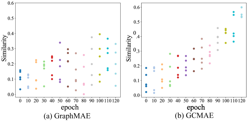
Figure 4. The embedding similarity between a node and its 5-hop neighbors w.r.t. the number of training epochs.

5.2. Accuracy for the Graph Tasks (RQ1)

Node classification. Table 4 reports the accuracy scores of our GCMAE and the baselines for node classification. We observe that GCMAE is the most accurate method on all datasets, and compared with the best baseline, the accuracy improvements of GCMAE  are 1.7% on Cora, 2.2% on Citeseer, 2.0% on PubMed, and 2.1% on Reddit. Considering the baselines, the supervised methods (i.e., GCN and GAT) perform the worst because they can only utilize label information while the other methods use self-supervised learning to introduce more supervision signals. The graph MAE methods generally perform better than the contrastive methods because node classification relies on the local information of each node (i.e., a local task), and graph MAE is better at capturing local information by learning to reconstruct individual node features and masked edges. Similar pattern is also observed in the results of other local tasks, i.e., link prediction and node clustering. The fact that GCMAE outperforms both contrastive and MAE methods suggests that our model designs allow us to enjoy the benefits of both paradigms.

Link prediction. Following SeeGera (Li et al., 2023b), S2GAE (Tan et al., 2023), we do not report the results of supervised methods for link prediction. Since DGI (Velickovic et al., 2019), MVGRL (Hassani and Khasahmadi, 2020), and GraphMAE (Hou et al., 2022) do not report relevant experimental results, we train a network for each of them and output prediction results.

The results of the link prediction are shown in Table 5. GCMAE  achieves the best prediction results (except AP on PubMEd), with an average improvement of 1.1% on AUC and 0.8% when compared to the runner-up MaskGAE. The performance of GCMAE  exceeds all contrastive methods by a large margin, with an average increase of 5.9% in AUC and 5.6% in AP. Compared to contrastive methods, we use adjacency matrix reconstruction as part of the total objective, forcing the model to pay more attention to graph structures. GraphMAE (Hou et al., 2022) performs poorly on link prediction, which indicates that only reconstructing node features can lead to performance degradation on link-level tasks. In contrast, MaskMAE (Li et al., 2022b) takes edges as reconstruction objectives, which is consistent with downstream tasks, and unsurprisingly becomes the strongest method among all baselines. Based on the observation, the adjacency matrix reconstruction brings more performance improvement to link prediction than edge reconstruction, because the model can capture more meaningful global structures of the graph.

Table 8. Node classification accuracy when using different designs for the encoder of GCMAE .

	Cora	Citeseer	PubMed
MAE Encoder	84.14	73.17	81.83
Con. Encoder	68.46	60.46	57.61
Fusion Encoder	85.61	71.71	78.63
Shared Encoder	88.82	76.77	88.51

Node clustering. As shown in Table 6, GCMAE  achieves the best results among all baselines on the node clustering task. Especially on Citeseer, GCMAE  improves by 2.2% on Reddit w.r.t. ARI when compared to the runner-up approach MaskGAE (Li et al., 2022b). Compared with the MAE method, the improvements range from 0.2% to 3.2% regarding NMI and from 0.5% to 3.4% regarding ARI. Since GCMAE  can learn the feature and structure difference between nodes of different clusters from global information, which helps the model clarify the boundaries of clusters. We can observe that the performance gap between the contrastive method and the MAE method on node clustering is not large, unlike node classification and link prediction. This is because the goal of node clustering is to divide the data set into different clusters, in other words, maximizing the similarity of intra-cluster nodes and expanding the difference of inter-cluster nodes. This goal is similar to the intrinsic mechanism of CL. Moreover, we choose 3 deep node clustering methods as the baseline, and GCMAE  can still achieve an average improvement of 10.5% in NMI and 11.4% in ARI. This means that we can obtain high-quality node embeddings for the node clustering task without deliberately tailoring a clustering loss to guide the training process.

Graph classification. SeeGera (Li et al., 2023b) and MaskGAE (Li et al., 2022b) are not chosen as baselines due to the unavailable source code. Table 7 reports all the experimental results for graph classification. We can see that the contrastive methods and the graph MAE methods have comparable performance in graph classification, each achieving three runner-up results. In contrast, GCMAE  achieves the highest accuracy on all datasets when compared to all baselines, the accuracy of our method is improved by an average of 1.3%. Our method benefits from both MAE and CL, and therefore can effectively distinguish the differences between graph-level embeddings by comparing multiple corrupted views. Compared to GraphMAE (Hou et al., 2022), by enhancing the feature discrimination through discrimination loss, our proposed method is able to learn meaningful representations even from features with limited information content, such as one-hot vectors based on labels or degrees. Overall, GCMAE  does not only excel on node-level (i.e., node classification and node clustering) and link-level (i.e., link prediction) tasks, and it can generalize well to graph-level downstream tasks. The results clearly demonstrate the effectiveness of the proposed GCMAE  framework and validate our claims.

5.3. Anatomy of the Design Goals (RQ2)

GCMAE  learns global information. To verify whether CL can help graph MAE to obtain global information, we visualize the similarity between nodes in GraphMAE and our GCMAE , respectively. Specifically, we randomly select distant nodes 5 hops away from the target node and then calculate the similarity between them. We can observe that as the training epoch increases, the similarity of target nodes to distant nodes remains at a low level, which means that MAE is prone to learn node embeddings from local information, according to the result shown in Figure 4 (a). When we combine the CL and graph MAE, GCMAE  can gradually improve the similarity between target nodes to distant nodes. In other words, CL can make up for the shortcoming of GNN layers that are too shallow and potentially help graph MAE surpass the constraints of local receptive field and acquire global information, letting graph nodes gain useful knowledge from nodes or edges that are out of GNN’s aggregation scope.

Note that as the number of training epochs increases, the similarity between the target node and the distant node does not continue to increase. As shown in Figure 4, after a certain number of epochs (i.e., epoch=90), the similarity tends to be stable in (0.4-0.6). Therefore, the model will not face the over-smoothing issue.

The shared encoder effectively transfers global information. We study the impact of shared encoder and unshared encoder on our model to evaluate whether the shared encoder can pass global information. Therefore, we conduct the node classification on Cora, Citeseer, and PubMed with the different types of encoder, Table 8 presents the accuracy results. We can find that “MAE Encoder” outperforms the other two independently parameterized encoders by a significant margin, but does not surpass the shared-parameter encoder. Kindly note that only using “MAE Encoder” means our method degenerates to GraphMAE (Hou et al., 2022). The “Con. Encoder” does not perform as well as expected, which may be due to the excessive corruption of the input graph caused by a high mask ratio, leading to the failure of the contrastive encoder. “Fusion Encoder” represents the average sum of the embeddings generated by the “MAE Encoder” and “Con. Encoder”. Naturally, “Fusion Encoder” may suffer from collapsed contrastive encoder, which results in suboptimal results. This is particularly important that the “Shared Encoder” achieves the best classification performance, which means CL can convey global information to the MAE module through the shared-parameter encoder, aiding MAE in perceiving long-range node semantics.

5.4. The Training Efficiency of GCMAE (RQ3)

In order to study whether unifying CL and graph MAE will increase the training time consumption, we conduct node classification on 4 datasets: Cora, Citeseer, PubMed, and Reddit, and report the total time consumption. We choose CCA (Zhang et al., 2021b) with the best performance on node classification among the contrastive methods, backbone method GraphMAE (Hou et al., 2022) and MaskGAE (Li et al., 2022b) with the best performance among MAE methods as comparison methods. Table 9 shows the time consumption of all methods under the parameter setting with the highest node classification accuracy, that is, the sum of pre-training time and the fine-tuning time for downstream tasks.

Table 9. End-to-end training time of representative methods. “s” means seconds and “h” means hours.

Method	Cora	Citeseer	PubMed	Reddit
CCA-SSG	2.2(s)	1.9(s)	4.6(s)	0.8(h)
GraphMAE	152.8(s)	93.1(s)	1270.1(s)	18.2(h)
MaskGAE	26.3(s)	40.5(s)	52.7(s)	2.3(h)
GCMAE	28.6(s)	55.3(s)	508.9(s)	2.5(h)

We can observe that CCA-SSG has the least time consumption, which is due to the use of canonical correlation analysis to optimize the calculation between the embeddings of the two views, which greatly reduces the time consumption caused by large matrix operations. Our GCMAE  is on average 2$\times$ faster than GraphMAE. This is because GraphMAE uses GAT (Veličković et al., 2017) as an encoder, and GAT needs to take the entire adjacency matrix as input when encoding the input graph. Even if we try to reduce the dimension of the hidden embeddings, it still introduces unacceptable time consumption when encountering large-scale graphs (e.g., Reddit with millions of nodes). Unlike GraphMAE, the overall time consumption of our method is similar to that of MaskGAE, because we both use GraphSAGE (Hamilton et al., 2017) to encode node embeddings, which can sample multiple subgraphs from a large-scale graph for mini-batch training without inputting the entire graph into the network. However, our method is still slower than MaskGAE, because we reconstruct the entire adjacency matrix instead of only reconstructing partial edges like MaskGAE. Overall, the efficiency performance of GCMAE is comparable to prior works, and there is not a significant increase in time consumption due to the combination of graph MAE and CL.

Table 10. Node classification accuracy when removing the key components of GCMAE.

	Cora	Citeseer	PubMed
GCMAE	88.8	76.7	88.5
w/o Contrast.	87.3	75.7	87.4
w/o Stru. Rec.	86.0	73.5	86.7
w/o Disc. Loss	87.0	74.1	86.9
GraphMAE	85.5	72.5	82.5

5.5. Ablation Study and Parameters (RQ4)

In this part, we conduct an ablation study for the designs of GCMAE  and explore the influence of the parameters. We experiment with the task of node classification and note that the observations are similar for the other graph tasks.

The components of GCMAE. To study the effectiveness of each component, we compare our complete framework with GraphMAE (Hou et al., 2022) and three variants: “w/o Con.”, “w/o Stru. Rec.” and “w/o Disc.”. The results are presented in Table 10, where “w/o Con.” means the removal of the CL loss, “w/o Stru. Rec.” is our method without adjacency matrix reconstruction, and “w/o Disc.” is our method without feature discrimination loss. All results correspond to the accuracy values (%) of node classification tasks on 3 benchmark datasets: Cora, Citeseer, and PubMed. We can find that the removal of any of these components leads to a decrease in performance. In particular, the exclusion of adjacency matrix reconstruction has the most severe impact on the model, resulting in a decrease of 3.2% in Cora, 4.3% in Citeseer, and 2.4% in PubMed. Interestingly, even if we totally remove the contrastive module, our method still outperforms the GraphMAE (Hou et al., 2022). This is because the adjacency matrix reconstruction provides rich graph structure information and the discrimination loss improves the feature discrimination among nodes. In other words, adjacency matrix reconstruction and discrimination loss play an extremely crucial role in our framework. In summary, all the above three components contribute significantly to the final results.

Effect of the hyper-parameters. To study the influence of different hyper-parameter settings on the model, we conduct sensitivity experiments on mask rate and drop rate in GCMAE. We report the performance in Figure 5, where the $x$-axis, $y$-axis, and $z$-axis represent the feature mask rate $p_{mask}$, the drop node rate $p_{drop}$, and the F1-Score value, respectively. We can find that the variation trends on all datasets are consistent. When $p_{mask}$ is large (0.5-0.8), the model performance remains within a satisfactory range, which can also be observed in previous graph MAE models. A higher mask rate means lower redundancy, in which can help the encoder recover missing node features from the few neighboring nodes. When $p_{mask}$ is fixed, increasing $p_{drop}$ can improve the classification accuracy. Overall, compared to $p_{drop}$, $p_{mask}$ plays a decisive role in model performance, the variation of $p_{mask}$ directly affects the experiment performance, while changes in $p_{drop}$ do not cause significant fluctuations in the final results.

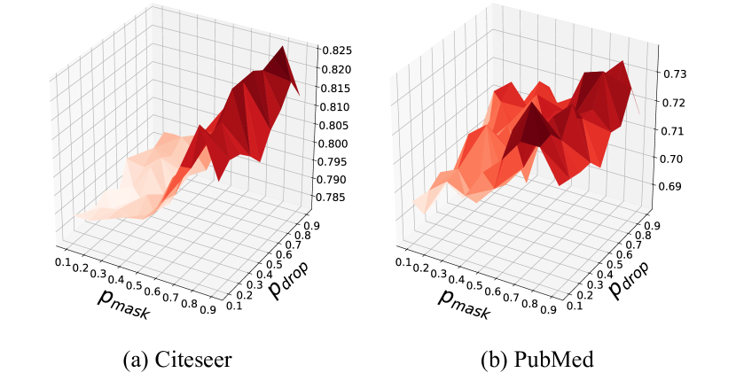
Figure 5. The influence of edge mask rate $p_{mask}$ and node drop node rate $p_{drop}$ on the performance of node classification.

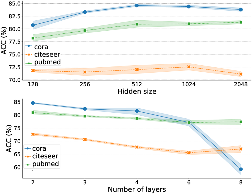
Figure 6. The influence of the hidden layer dimension and the number of layers in the GNN models on the accuracy of our GCMAE  for node classification.

The impact of network width and depth on performance has attracted significant attention in the CL methods (Zhu et al., 2020; Mo et al., 2022). Therefore, we investigate the effects of selecting multiple network scale parameters on our model. As shown in Figure 6, increasing the network width results in a performance improvement of approximately 5.9% in Cora, 3.1% in Citesser, and 4.0% in PubMed, as long as the hidden size does not exceed 1024 (except for PubMed where the limit is 2048). In contrast, a smaller hidden size leads to a sharp drop in performance. GCMAE achieves the best performance on most benchmarks with a 512-dimensional embedding. This means a moderate hidden size is crucial for the model to learn informative and compact node embeddings for downstream tasks.

Meanwhile, we can observe that network depth has a relatively smaller impact on performance compared to network width. Figure 6 shows that when the network has 2 layers, the accuracy is highest across all datasets. As the depth increases, the performance gradually decreases, with a decline of 30.0% in Cora, 7.8% in Citeseer, and 3.5% in PubMed when the depth reaches 8. Surprisingly, GNNs like GIN and GAT achieve good results with shallow depths, contrary to empirical results in the field of computer vision (He et al., 2022). This may be due to the fact that deep GNNs are challenging to optimize. As the depth increases, the learned representations tend to become homogeneous, thus degrading the performance.

6. Related Work

In this part, we review representative works on contrastive and generative methods for graph self-supervised learning (GSSL).

6.1. Contrastive Methods for Graph SSL

Inspired by the success of CL in computer vision and natural language processing  (Chen et al., 2020a; Gao et al., 2021b; He et al., 2020), many works develop constrative methods for graph learning (Velickovic et al., 2019; Hassani and Khasahmadi, 2020; Zhu et al., 2020; Xia et al., 2021; Li et al., 2023a). These methods generally produce multiple corrupted views of the graph via data augmentation and maximize the similarity between these views. For instance, GraphCL (You et al., 2020) adopts four types of graph augmentations (i.e., node dropping, edge perturbation, attribute masking, and subgraph sampling) to incorporate different priors and learns to predict whether two graphs are generated from the same graph. To improve GraphCL, GCA (Zhu et al., 2021) determines the importance of each node via its centrality and decides whether to mask a node according to its importance. The node with higher centrality is less likely to be masked. BGRL (Thakoor et al., 2021) proposes to conduct CL without negative samples and thus reduces model training time. DGI (Velickovic et al., 2019) conducts CL using patches of a graph and uses a read-out function to compute graph-level embedding from the node embeddings. GRACE (Zhu et al., 2020) corrupts both the graph topology and the node features such that contrast learning can capture more information. MVGRL (Hassani and Khasahmadi, 2020) observes that simply increasing the number of views does not improve performance and proposes to maximize the mutual information among the node and graph representations in different views. CCA-SSG (Zhang et al., 2021b) leverages canonical correlation analysis to speedup the computation of contrastive loss among multiple augmented views and reduce model training time. We observe that the contrastive methods are good at capturing global information of the graph but poor in learning the local information for particular edges and nodes. Thus, by augmenting MAE with CL, our GCMAE outperforms the existing GSSL methods.

6.2. Generative SSL Method

Different from contrastive methods, generative methods aim to reconstruct input data from hidden embeddings via a decoder and then minimize the distance between the input graph and the reconstructed graph.

Graph Autoencoder (GAE) is a classical self-supervised learning method, which encodes the graph structure information into a low-dimensional latent space and then reconstructs the adjacency matrix from hidden embeddings (Wang et al., 2017; Salehi and Davulcu, 2019; Cao et al., 2016). For example, DNGR (Cao et al., 2016) uses a stacked denoising autoencoder (Vincent et al., 2008) to encode and decode the PPMI matrix via multi-layer perceptrons. However, DNGR ignores the feature information when encoding node embeddings. Therefore, GAE (Kipf and Welling, 2016b) utilizes GCN (Kipf and Welling, 2016a) to encode node structural information and node feature information at the same time and then uses a dot-product operation for reconstructing the input graph. Variational GAE (VGAE) (Kipf and Welling, 2016b) learns the distribution of data, where KL divergence is used to measure the distance between the empirical distribution and the prior distribution. In order to further narrow the gap between the above two distributions, ARVGA (Pan et al., 2018) employs the training scheme of a generative adversarial network (Goodfellow et al., 2014) to address the approximate problem. RGVAE (Ma et al., 2018) further imposes validity constraints on a graph variational autoencoder to regularize the output distribution of the decoder. Unlike the previous asymmetric decoder structure, GALA (Park et al., 2019) builds a fully symmetric decoder, which facilitates the proposed autoencoder architecture to make use of the graph structure. Later studies focused on leveraging feature reconstruction or additional auxiliary information (Pan et al., 2018; Salehi and Davulcu, 2019). Unfortunately, most of them mainly perform well on a single task such as node classification or link prediction, since they are limited by a sufficient reconstruction objective. However, our GCMAE  surpasses these GAE methods on various downstream tasks due to both reconstructing node features and edge.

Masked Autoencoders learn graph representations by masking certain nodes or edges and then reconstructing the masked tokens (Hu et al., 2020; Zhang et al., 2021a; Hou et al., 2023). This strategy allows the graph to use its own structure and feature information in a self-supervised manner without expensive label annotations. Recently, GraphMAE (Hou et al., 2022) enforces the model to reconstruct the original graph from redundant node features by masking node features and applying a re-masking strategy before a GNN decoder. Instead of masking node features, MaskGAE (Li et al., 2022b) selects edges as the masked token and then reconstructs the graph edges or random masked path accordingly. MaskGAE achieves superior performance in link prediction tasks compared to other graph MAE methods, but its performance in classification tasks is not as satisfactory as feature-based MAE because it does not reconstruct the node features. S2GAE (Tan et al., 2023) proposes a cross-correlation decoder to explicitly capture the similarity of the relationship between two connected nodes at different granularities. SeeGera (Li et al., 2023b) is a hierarchical variational framework that jointly embeds nodes and features in the encoder and reconstructs links and features in the decoder, where an additional structure/feature masking layer is added to improve the generalization ability of the model. Based on the above observations, these graph MAE methods all suffer from inaccessible global information, resulting in sub-optimal performance. However, GCMAE  surpasses these graph MAE methods, as unifying CL and graph MAE enjoys the benefits of both paradigms and yields more high-quality node embeddings.

7. CONCLUSION

In this paper, we observed that the two main paradigms for graph self-supervised learning, i.e., masked autoencoder and contrastive learning, have their own limitations but complement each other. Thus, we proposed the GCMAE framework to jointly utilize MAE and contrastive learning for enhanced performance. GCMAE  comes with tailored model designs including a shared encoder for information exchange, discrimination loss to tackle feature smoothing, and adjacency matrix reconstruction to learn global information of the graph. We conducted extensive experiments to evaluate GCMAE on various graph tasks. The results show that GCMAE  outperforms state-of-the-art GSSL methods by a large margin and is general across graph tasks.

References

- (1)
- Arthur and Vassilvitskii (2006) David Arthur and Sergei Vassilvitskii. 2006. How slow is the k-means method?. In Proceedings of the Twenty-second Annual Symposium on Computational Geometry. 144–153.
- Cai et al. (2023) Xuheng Cai, Chao Huang, Lianghao Xia, and Xubin Ren. 2023. LightGCL: Simple Yet Effective Graph Contrastive Learning for Recommendation. arXiv preprint arXiv:2302.08191 (2023).
- Cao et al. (2016) Shaosheng Cao, Wei Lu, and Qiongkai Xu. 2016. Deep neural networks for learning graph representations. In Proceedings of the AAAI conference on Artificial Intelligence, Vol. 30.
- Chang and Lin (2011) Chih-Chung Chang and Chih-Jen Lin. 2011. LIBSVM: a library for support vector machines. ACM Transactions on Intelligent Systems and Technology (TIST) 2, 3 (2011), 1–27.
- Chen et al. (2020b) Deli Chen, Yankai Lin, Wei Li, Peng Li, Jie Zhou, and Xu Sun. 2020b. Measuring and relieving the over-smoothing problem for graph neural networks from the topological view. In Proceedings of the AAAI Conference on Artificial Intelligence, Vol. 34. 3438–3445.
- Chen et al. (2023a) Jiazun Chen, Jun Gao, and Bin Cui. 2023a. ICS-GNN+: lightweight interactive community search via graph neural network. The VLDB Journal 32, 2 (2023), 447–467.
- Chen et al. (2023b) Jiazun Chen, Yikuan Xia, and Jun Gao. 2023b. CommunityAF: An Example-Based Community Search Method via Autoregressive Flow. Proceedings of the VLDB Endowment 16, 10 (2023), 2565–2577.
- Chen et al. (2020a) Ting Chen, Simon Kornblith, Mohammad Norouzi, and Geoffrey Hinton. 2020a. A simple framework for contrastive learning of visual representations. In International Conference on Machine Learning. 1597–1607.
- Chien et al. (2021) Eli Chien, Wei-Cheng Chang, Cho-Jui Hsieh, Hsiang-Fu Yu, Jiong Zhang, Olgica Milenkovic, and Inderjit S Dhillon. 2021. Node feature extraction by self-supervised multi-scale neighborhood prediction. arXiv preprint arXiv:2111.00064 (2021).
- Cui et al. (2021) Yue Cui, Kai Zheng, Dingshan Cui, Jiandong Xie, Liwei Deng, Feiteng Huang, and Xiaofang Zhou. 2021. METRO: a generic graph neural network framework for multivariate time series forecasting. Proceedings of the VLDB Endowment 15, 2 (2021), 224–236.
- Dai et al. (2018) Hanjun Dai, Zornitsa Kozareva, Bo Dai, Alex Smola, and Le Song. 2018. Learning steady-states of iterative algorithms over graphs. In International Conference on Machine Learning. 1106–1114.
- Fettal et al. (2022) Chakib Fettal, Lazhar Labiod, and Mohamed Nadif. 2022. Efficient graph convolution for joint node representation learning and clustering. In Proceedings of the Fifteenth ACM International conference on Web Search and Data Mining. 289–297.
- Gao et al. (2021a) Jun Gao, Jiazun Chen, Zhao Li, and Ji Zhang. 2021a. ICS-GNN: lightweight interactive community search via graph neural network. Proceedings of the VLDB Endowment 14, 6 (2021), 1006–1018.
- Gao et al. (2021b) Tianyu Gao, Xingcheng Yao, and Danqi Chen. 2021b. Simcse: Simple contrastive learning of sentence embeddings. arXiv preprint arXiv:2104.08821 (2021).
- Goodfellow et al. (2014) Ian Goodfellow, Jean Pouget-Abadie, Mehdi Mirza, Bing Xu, David Warde-Farley, Sherjil Ozair, Aaron Courville, and Yoshua Bengio. 2014. Generative adversarial nets. Advances in Neural Information Processing Systems 27 (2014).
- Guo and Dai (2022) Lin Guo and Qun Dai. 2022. Graph clustering via variational graph embedding. Pattern Recognition 122 (2022), 108334.
- Hamilton et al. (2017) Will Hamilton, Zhitao Ying, and Jure Leskovec. 2017. Inductive representation learning on large graphs. Advances in Neural Information Processing Systems 30 (2017).
- Hassani and Khasahmadi (2020) Kaveh Hassani and Amir Hosein Khasahmadi. 2020. Contrastive multi-view representation learning on graphs. In International Conference on Machine Learning. 4116–4126.
- He et al. (2022) Kaiming He, Xinlei Chen, Saining Xie, Yanghao Li, Piotr Dollár, and Ross Girshick. 2022. Masked autoencoders are scalable vision learners. In Proceedings of the IEEE/CVF Conference on Computer Vision and Pattern Recognition. 16000–16009.
- He et al. (2020) Kaiming He, Haoqi Fan, Yuxin Wu, Saining Xie, and Ross Girshick. 2020. Momentum contrast for unsupervised visual representation learning. In Proceedings of the IEEE/CVF Conference on Computer Vision and Pattern Recognition. 9729–9738.
- Hou et al. (2023) Zhenyu Hou, Yufei He, Yukuo Cen, Xiao Liu, Yuxiao Dong, Evgeny Kharlamov, and Jie Tang. 2023. GraphMAE2: A Decoding-Enhanced Masked Self-Supervised Graph Learner. arXiv preprint arXiv:2304.04779 (2023).
- Hou et al. (2022) Zhenyu Hou, Xiao Liu, Yukuo Cen, Yuxiao Dong, Hongxia Yang, Chunjie Wang, and Jie Tang. 2022. Graphmae: Self-supervised masked graph autoencoders. In Proceedings of the 28th ACM SIGKDD Conference on Knowledge Discovery and Data Mining. 594–604.
- Hu et al. (2019) Weihua Hu, Bowen Liu, Joseph Gomes, Marinka Zitnik, Percy Liang, Vijay Pande, and Jure Leskovec. 2019. Strategies for pre-training graph neural networks. arXiv preprint arXiv:1905.12265 (2019).
- Hu et al. (2020) Ziniu Hu, Yuxiao Dong, Kuansan Wang, Kai-Wei Chang, and Yizhou Sun. 2020. Gpt-gnn: Generative pre-training of graph neural networks. In Proceedings of the 26th ACM SIGKDD International Conference on Knowledge Discovery and Data Mining. 1857–1867.
- Huang et al. (2022) Zhicheng Huang, Xiaojie Jin, Chengze Lu, Qibin Hou, Ming-Ming Cheng, Dongmei Fu, Xiaohui Shen, and Jiashi Feng. 2022. Contrastive masked autoencoders are stronger vision learners. arXiv preprint arXiv:2207.13532 (2022).
- Jin et al. (2020) Wei Jin, Tyler Derr, Haochen Liu, Yiqi Wang, Suhang Wang, Zitao Liu, and Jiliang Tang. 2020. Self-supervised learning on graphs: Deep insights and new direction. arXiv preprint arXiv:2006.10141 (2020).
- Kipf and Welling (2016a) Thomas N Kipf and Max Welling. 2016a. Semi-supervised classification with graph convolutional networks. arXiv preprint arXiv:1609.02907 (2016).
- Kipf and Welling (2016b) Thomas N Kipf and Max Welling. 2016b. Variational Graph Auto-Encoders. NIPS Workshop on Bayesian Deep Learning (2016).
- Kong and Zhang (2023) Xiangwen Kong and Xiangyu Zhang. 2023. Understanding masked image modeling via learning occlusion invariant feature. In Proceedings of the IEEE/CVF Conference on Computer Vision and Pattern Recognition. 6241–6251.
- Li et al. (2022b) Jintang Li, Ruofan Wu, Wangbin Sun, Liang Chen, Sheng Tian, Liang Zhu, Changhua Meng, Zibin Zheng, and Weiqiang Wang. 2022b. MaskGAE: masked graph modeling meets graph autoencoders. arXiv preprint arXiv:2205.10053 (2022).
- Li et al. (2022a) Sihang Li, Xiang Wang, An Zhang, Yingxin Wu, Xiangnan He, and Tat-Seng Chua. 2022a. Let invariant rationale discovery inspire graph contrastive learning. In International Conference on Machine Learning. PMLR, 13052–13065.
- Li et al. (2023a) Wen-Zhi Li, Chang-Dong Wang, Hui Xiong, and Jian-Huang Lai. 2023a. HomoGCL: Rethinking Homophily in Graph Contrastive Learning. arXiv preprint arXiv:2306.09614 (2023).
- Li et al. (2023b) Xiang Li, Tiandi Ye, Caihua Shan, Dongsheng Li, and Ming Gao. 2023b. SeeGera: Self-supervised Semi-implicit Graph Variational Auto-encoders with Masking. In Proceedings of the ACM Web Conference 2023. 143–153.
- Liu et al. (2020) Sicen Liu, Tao Li, Haoyang Ding, Buzhou Tang, Xiaolong Wang, Qingcai Chen, Jun Yan, and Yi Zhou. 2020. A hybrid method of recurrent neural network and graph neural network for next-period prescription prediction. International Journal of Machine Learning and Cybernetics 11 (2020), 2849–2856.
- Liu et al. (2021) Yang Liu, Xiang Ao, Zidi Qin, Jianfeng Chi, Jinghua Feng, Hao Yang, and Qing He. 2021. Pick and choose: a GNN-based imbalanced learning approach for fraud detection. In Proceedings of the Web Conference 2021. 3168–3177.
- Liu et al. (2023) Yue Liu, Xihong Yang, Sihang Zhou, Xinwang Liu, Siwei Wang, Ke Liang, Wenxuan Tu, and Liang Li. 2023. Simple contrastive graph clustering. IEEE Transactions on Neural Networks and Learning Systems (2023).
- Lu et al. (2022) Mingxuan Lu, Zhichao Han, Susie Xi Rao, Zitao Zhang, Yang Zhao, Yinan Shan, Ramesh Raghunathan, Ce Zhang, and Jiawei Jiang. 2022. BRIGHT-Graph Neural Networks in Real-Time Fraud Detection. In Proceedings of the 31st ACM International Conference on Information and Knowledge Management. 3342–3351.
- Ma et al. (2018) Tengfei Ma, Jie Chen, and Cao Xiao. 2018. Constrained generation of semantically valid graphs via regularizing variational autoencoders. Advances in Neural Information Processing Systems 31 (2018).
- Ma et al. (2021) Yi Ma, Ying Chen, Yiran Tian, Chenjie Gu, and Tao Jiang. 2021. Contrastive study of in situ sensing and swabbing detection based on SERS-active gold nanobush–PDMS hybrid film. Journal of Agricultural and Food Chemistry 69, 6 (2021), 1975–1983.
- Mo et al. (2022) Yujie Mo, Liang Peng, Jie Xu, Xiaoshuang Shi, and Xiaofeng Zhu. 2022. Simple unsupervised graph representation learning. In Proceedings of the AAAI Conference on Artificial Intelligence, Vol. 36. 7797–7805.
- Pan et al. (2018) Shirui Pan, Ruiqi Hu, Guodong Long, Jing Jiang, Lina Yao, and Chengqi Zhang. 2018. Adversarially regularized graph autoencoder for graph embedding. arXiv preprint arXiv:1802.04407 (2018).
- Park et al. (2019) Jiwoong Park, Minsik Lee, Hyung Jin Chang, Kyuewang Lee, and Jin Young Choi. 2019. Symmetric graph convolutional autoencoder for unsupervised graph representation learning. In Proceedings of the IEEE/CVF International Conference on Computer Vision. 6519–6528.
- Qi et al. (2023) Zekun Qi, Runpei Dong, Guofan Fan, Zheng Ge, Xiangyu Zhang, Kaisheng Ma, and Li Yi. 2023. Contrast with Reconstruct: Contrastive 3D Representation Learning Guided by Generative Pretraining. arXiv preprint arXiv:2302.02318 (2023).
- Sahu et al. (2020) Siddhartha Sahu, Amine Mhedhbi, Semih Salihoglu, Jimmy Lin, and M Tamer Özsu. 2020. The ubiquity of large graphs and surprising challenges of graph processing: extended survey. The VLDB journal 29 (2020), 595–618.
- Salehi and Davulcu (2019) Amin Salehi and Hasan Davulcu. 2019. Graph attention auto-encoders. arXiv preprint arXiv:1905.10715 (2019).
- Sun et al. (2019) Fan-Yun Sun, Jordan Hoffmann, Vikas Verma, and Jian Tang. 2019. Infograph: Unsupervised and semi-supervised graph-level representation learning via mutual information maximization. arXiv preprint arXiv:1908.01000 (2019).
- Tan et al. (2023) Qiaoyu Tan, Ninghao Liu, Xiao Huang, Soo-Hyun Choi, Li Li, Rui Chen, and Xia Hu. 2023. S2GAE: Self-Supervised Graph Autoencoders are Generalizable Learners with Graph Masking. In Proceedings of the Sixteenth ACM International Conference on Web Search and Data Mining. 787–795.
- Thakoor et al. (2021) Shantanu Thakoor, Corentin Tallec, Mohammad Gheshlaghi Azar, Rémi Munos, Petar Veličković, and Michal Valko. 2021. Bootstrapped representation learning on graphs. In ICLR 2021 Workshop on Geometrical and Topological Representation Learning.
- Veličković et al. (2017) Petar Veličković, Guillem Cucurull, Arantxa Casanova, Adriana Romero, Pietro Lio, and Yoshua Bengio. 2017. Graph attention networks. arXiv preprint arXiv:1710.10903 (2017).
- Velickovic et al. (2019) Petar Velickovic, William Fedus, William L Hamilton, Pietro Liò, Yoshua Bengio, and R Devon Hjelm. 2019. Deep graph infomax. The International Conference on Learning Representations 2, 3 (2019), 4.
- Vincent et al. (2008) Pascal Vincent, Hugo Larochelle, Yoshua Bengio, and Pierre-Antoine Manzagol. 2008. Extracting and composing robust features with denoising autoencoders. In Proceedings of the 25th International Conference on Machine Learning. 1096–1103.
- Wang et al. (2017) Chun Wang, Shirui Pan, Guodong Long, Xingquan Zhu, and Jing Jiang. 2017. Mgae: Marginalized graph autoencoder for graph clustering. In Proceedings of the 2017 ACM on Conference on Information and Knowledge Management. 889–898.
- Wei et al. (2022) Chen Wei, Haoqi Fan, Saining Xie, Chao-Yuan Wu, Alan Yuille, and Christoph Feichtenhofer. 2022. Masked feature prediction for self-supervised visual pre-training. In Proceedings of the IEEE/CVF Conference on Computer Vision and Pattern Recognition. 14668–14678.
- Wu et al. (2021) Lirong Wu, Haitao Lin, Cheng Tan, Zhangyang Gao, and Stan Z Li. 2021. Self-supervised learning on graphs: Contrastive, generative, or predictive. IEEE Transactions on Knowledge and Data Engineering (2021).
- Xia et al. (2021) Jun Xia, Lirong Wu, Ge Wang, Jintao Chen, and Stan Z Li. 2021. Progcl: Rethinking hard negative mining in graph contrastive learning. arXiv preprint arXiv:2110.02027 (2021).
- Xu et al. (2021) Dongkuan Xu, Wei Cheng, Dongsheng Luo, Haifeng Chen, and Xiang Zhang. 2021. Infogcl: Information-aware graph contrastive learning. Advances in Neural Information Processing Systems 34 (2021), 30414–30425.
- Yin et al. (2022) Yihang Yin, Qingzhong Wang, Siyu Huang, Haoyi Xiong, and Xiang Zhang. 2022. Autogcl: Automated graph contrastive learning via learnable view generators. In Proceedings of the AAAI Conference on Artificial Intelligence, Vol. 36. 8892–8900.
- You et al. (2021) Yuning You, Tianlong Chen, Yang Shen, and Zhangyang Wang. 2021. Graph contrastive learning automated. In International Conference on Machine Learning. PMLR, 12121–12132.
- You et al. (2020) Yuning You, Tianlong Chen, Yongduo Sui, Ting Chen, Zhangyang Wang, and Yang Shen. 2020. Graph contrastive learning with augmentations. Advances in Neural Information Processing Systems 33 (2020), 5812–5823.
- Zhang et al. (2021b) Hengrui Zhang, Qitian Wu, Junchi Yan, David Wipf, and Philip S Yu. 2021b. From canonical correlation analysis to self-supervised graph neural networks. Advances in Neural Information Processing Systems 34 (2021), 76–89.
- Zhang et al. (2021a) Shichang Zhang, Yozen Liu, Yizhou Sun, and Neil Shah. 2021a. Graph-less neural networks: Teaching old mlps new tricks via distillation. arXiv preprint arXiv:2110.08727 (2021).
- Zhang et al. (2020) Wentao Zhang, Xupeng Miao, Yingxia Shao, Jiawei Jiang, Lei Chen, Olivier Ruas, and Bin Cui. 2020. Reliable data distillation on graph convolutional network. In Proceedings of the 2020 ACM SIGMOD International Conference on Management of Data. 1399–1414.
- Zhao and Akoglu (2019) Lingxiao Zhao and Leman Akoglu. 2019. Pairnorm: Tackling oversmoothing in gnns. arXiv preprint arXiv:1909.12223 (2019).
- Zheng et al. (2022) Chenguang Zheng, Hongzhi Chen, Yuxuan Cheng, Zhezheng Song, Yifan Wu, Changji Li, James Cheng, Hao Yang, and Shuai Zhang. 2022. ByteGNN: efficient graph neural network training at large scale. Proceedings of the VLDB Endowment 15, 6 (2022), 1228–1242.
- Zhu et al. (2020) Yanqiao Zhu, Yichen Xu, Feng Yu, Qiang Liu, Shu Wu, and Liang Wang. 2020. Deep graph contrastive representation learning. arXiv preprint arXiv:2006.04131 (2020).
- Zhu et al. (2021) Yanqiao Zhu, Yichen Xu, Feng Yu, Qiang Liu, Shu Wu, and Liang Wang. 2021. Graph contrastive learning with adaptive augmentation. In Proceedings of the Web Conference 2021. 2069–2080.