Covert communication with Gaussian noise: from random access channel to point-to-point channel

Abstract

We propose a covert communication protocol for the spread-spectrum multiple random access with additive white Gaussian noise (AWGN) channel. No existing paper has studied covert communication for the random access channel. Our protocol assumes binary discrete phase-shift keying (BPSK) modulation, and it works well under imperfect channel state information (I-CSI) for both the legitimate and adversary receivers, which is a realistic assumption in the low power regime. Also, our method assumes that the legitimate users share secret variables in a similar way as the preceding studies. Although several studies investigated the covert communication for the point-to-point communication, no existing paper considers the covert communication under the above uncertainty assumption even for point-to-point communication. Our protocol under the above uncertainty assumption allows $O(n)$ legitimate senders and $O(n/\log n)$ active legitimate senders. Furthermore, our protocol can be converted to a protocol for point-to-point communication that works under the above uncertainty assumption.

I Introduction

I-A Background: point-to-point covert communication

Covert communication is a technology to hide the existence of communication, and has been actively studied. This type of communication is often called communication with low probability of detection. In this technology, the legitimate sender intends to transmit an information message to the legitimate receiver while making such communication undetectable by the adversary. This task can be achieved when adversary’s observation with the silent case is imitated by adversary’s observation under the existence of a communication between the legitimate sender and the legitimate receiver. In fact, when the output of the silent case is written as a convex combination of other outputs in the channel to the adversary, the above task can be easily achieved. Here, we call this condition the redundant condition, and its rigorous definition is given in Section III-C. Under the above condition, using the method of wire-tap channel [1, 2, 3], the papers [4, 5] consider this problem for the point-to-point channel under the discrete memoryless condition. They showed that the covert transmission length $O(n)$ is possible with $n$ uses of the channel. The idea of this method is that the transmitter transmits an independent and identically distributed (i.i.d.) sequence for the no-communication mode, which makes the problem more similar to covert communication in the presence of a jammer as discussed in [6, Remark 2].

However, the redundant condition does not hold in general. For example, when the form of the channel to the adversary is known, the additive white Gaussian noise (AWGN) channel and the binary symmetric channel (BSC) do not satisfy this condition. The papers [7] and [8, 9] discussed this problem for the cases of AWGN and BSC, respectively. Then, the papers [5, 10] studied the covert communication problem under general discrete memoryless channel for the point-to-point channel when the redundant condition does not hold. They showed that the optimal covert transmission length is $O(\sqrt{n})$ in the non-redundant case with $n$ uses of the channel. Following these studies, the papers [11, 12, 13] studied this problem for AGWN as considering continuous time models. Also, the paper [14] extended this discussion to multiple-input multipl-output (MIMO) AWGN channels.

The fundamental assumption of the non-redundant case is using preshared secure keys between the legitimate sender and the legitimate receiver. Due to the preshared keys, the legitimate users can realize covert communication even when the channel to the adversary has smaller noise than the channel to the legitimate receiver. That is, to preshare keys is a mandatory resource for covert communication whenever Willie’s channel is not worse than Bob’s channel. Later, many subsequent studies [15, 16, 17, 18, 19, 20, 21, 22] analyzed the point-to-point covert communication over the AWGN channel under different additional assumptions.

Figure 1: This figure illustrates a random access channel with one legitimate receiver (Bob), one adversary (Willie), and multiple legitimate senders. Our protocol allows $O(n/\log n)$ active legitimate senders. Illegitimate receivers are shown in black.

I-B Background: random access channel

Our focus in this work is the random access channel where the point-to-point is a special case. A number of studies [23, 24, 25, 26, 27] have already discussed the random access channel from the viewpoint of information theory, however, these works do not address the covertness property of this channel. Recently, the paper [28] addressed the anti-jamming secrecy in the random access channel, but it did not discuss covertness. Another recent paper [29] discussed the covert communication for the access channel assuming discrete time, but it did not address random access channel nor AWGN channel.

I-C Problem statement and novelty

In this paper, we present an information theoretical study of the covertness of (direct sequence) random access and one time pad encryption. We assume BPSK modulation and novel assumptions on the channel knowledge by the legitimate users and the adversary, Willie. Furthermore, to realize covertness, depending on the legitimate sender, our method uses preshared secret binary symbols, which is often called secret chips. Fig. 1 shows its illustrative scenario and the relation with existing results for access channel are summarized as Table I clarifying the novelty of our work. Throughout this paper, we assume logarithms with base $e$.

TABLE I: Comparison with existing results for access channel

	Covertness	Random access	Type of
		channel	channel
[29]	Yes	No	Discrete
[23, 24, 27]	No	Yes	Discrete
[25, 26, 28]	No	Yes	AWGN
This paper	Yes	Yes	AWGN

In our setting, $n$ expresses the number of uses of the channel during one coding block-length. Our method allows $O(n)$ legitimate senders and $O(n/\log n)$ active legitimate senders under the assumption of preshared secure keys between these legitimate senders and the legitimate receiver. To achieve this performance, we pose a novel and realistic channel condition (in the low power regime) as follows because it is impossible to achieve covertness of $O(n/\log n)$ bits in the non-redundant case when the channel parameter is completely known to the adversary, i.e., the channel is identified by the adversary. In a realistic scenario, it is difficult for both legitimate and adversary parties to obtain a complete knowledge of the channel parameters. Therefore, it is natural to assume that all parties (legitimate and non-legitimate) do not have a complete knowledge of the channel parameters while we assume that the channel parameters are fixed during one coding block-length. The latter assumption is justified when our signal model and asymptotic results hold within the channel coherence time. Under the above realistic conditions for the uncertainty, our protocol guarantees that the legitimate receiver retrieves the message.

Another novelty in our formulation is the universality of our proposed codes. In information theory a code is called a universal code when the code does not depend on the channel parameter in the above way, i.e., our code construction does not require full knowledge of the channel [30, 31]. In our case, this means that our method allows the dispersion of signal intensities from the senders in the detection of both receivers due to the effect of the fading fluctuation. As a consequence, we make the realistic assumption that for a known scenario of interest, an upper and lower bound of the channel coefficients can be estimated.

In addition, our method assumes preshared secure keys between the legitimate sender and the legitimate receiver in the same way as [5, 10, 11, 12, 13] and it works even when the channel to the adversary has smaller noise than the channel to the legitimate receiver. That is, for every coding block, each legitimate sender shares secret binary symbols as pre-shared secrets with the legitimate receiver while the legitimate sender can send only one bit. Hence, when the senders need to transmit $\ell$ bits, it is sufficient that they repeat this protocol $\ell$ times. In practice, this is realistically achieved using well known and widely available spreading codes. Each legitimate sender has $n$ different preshared secret binary symbols. That is, the number of secret binary symbols at the legitimate receiver is $n$ times the number of legitimate senders.

Our encoder is very simple for random access channel. That is, when a legitimate sender is active and intends to transmit one bit $X$, the sender encodes the intended bit $X$ into $n$ channel inputs by using one time pad encryption with $n$ preshared secret binary symbols. Then, the legitimate receiver recovers the transmitted bits by using the preshared secret bits.

The most novel point of our work is the covertness analysis for the adversary. In our analysis, the covertness evaluation is reduced to the difference between the Gaussian distribution and the distribution of the weighted sample mean of $n$ independent random variables subject to the average output distribution of BPSK modulation. Although a variant of the central limit theorem [32] guarantees that the distribution of the weighted sample mean of $n$ independent random variables approaches to a Gaussian distribution, our covertness analysis needs the evaluation of the variational distance between the above two distributions. When the fading coefficients from a sender in Willie’s detection does not depend on the sender, it is sufficient to discuss the variational distance between the distribution of the sample mean and a Gaussian distribution. Such a case was discussed in [33, (1.3)]. However, the general case requires more difficult analysis. Fortunately, the recent papers [34, 35] have studied this mathematical problem by using Poincaré constant [34, 35, 36, 37]. Applying this result, we derive our covertness analysis.

I-D From random access channel protocol to point-to-point channel

Another novelty of our work is that we consider the fact that our protocol can be converted to a protocol for point-to-point communication that works under the above assumptions. Under this conversion, we obtain a covert communication protocol for the point-to-point channel that has $\lceil(l_{n}+1)/2\rceil$ different values as the channel input power, and achieves the covert transmission of $O(n/\log n)$ bits, where $l_{n}$ is the number of bits the legitimate sender wants to transmit to the legitimate receiver. Although existing studies assuming the redundant case [4, 5] achieve covert transmission length $O(n)$ with $n$ uses of the channel, existing studies assuming the non-redundant case [5, 10, 11, 12, 13] achieve covert transmission length $O(\sqrt{n})$, which is much smaller than the transmission length of the conventional communication. To resolve this problem, many subsequent researchers [15, 16, 17, 18, 19, 20, 21, 22] introduced the uncertainty of the channel parameters only of the channel to the adversary under the AWGN channel. In fact, due to the uncertainty, the adversary cannot distinguish the output of the Gaussian mixture input distribution from the output of zero input. That is, this modification enables the channel model to satisfy the redundant condition, which leads the covert transmission length $O(n)$. However, these studies assume that the legitimate receiver knows the channel parameters of his/her own channel, which is an unequal assumption, i.e., an unrealistic assumption. To make a fair assumption, we pose the novel and realistic channel condition introduced above that the channel parameters of the AWGN channels to both the legitimate and adversary receivers present some uncertainty, i.e. are not completely known to them. Fortunately, our protocol on the point-to-point channel achieves the covert transmission of $O(n/\log n)$ bits when both receivers (the legitimate receiver and the adversary) have uncertainty in their detection. In this sense, our method has an advantage over existing methods even under the Gaussian point-to-point channel.

Finally, we remark that our main focus is the analysis of the asymptotic performance of our code to guarantee covertness and therefore practical issues such as BPSK symbol acquisition or outage probability (e.g for concrete statistics assumptions on the channel dynamics) and practical channel estimation are out of the scope of this work and is left for future work. The relation with existing results for point-to-point channel is summarized in Table II, clarifying the novelty of our work and results.

TABLE II: Comparison with existing results for point-to-point channel

	Transmission	Bob	Willie	Type
	length	knows	knows	of
		channel	channel	channel
		parameters	parameters
[10, 5]	$O(\sqrt{n})$	Yes	Yes	Discrete
[11–13]	$O(\sqrt{n})$	Yes	Yes	AWGN
[15–22]	$O(n)$	Yes	No	AWGN
This paper	$O(n/\log n)$	No	No	AWGN

$n$ is the number of uses of channel.

This paper is organized as follows. Section II describes our formulation of random access channel model, and states our result in this case. Section III explains what protocol is obtained for the particular case of point-to-point channel model. Then, Section III compares our obtained code for the point-to-point channel model with simple applications of the methods [4, 5]. Section IV shows that Bob correctly recovers the message with almost probability one under both models in the asymptotic case. Section V formulates covertness with respect to Willie, and states our covertness result. In addition, Section V shows its proof for the case with equal fading including the point-to-point channel model while its proof with the general case with unequal fading is shown in Appendix. Section VI presents a discussion of our results.

II Random access channel

II-A Random access channel model

Our random access channel model has $m$ senders ${\cal A}_{1},\ldots,{\cal A}_{m}$, one adversary, Willie, and the legitimate receiver, Bob. The task of our protocol is formulated as follows. Each sender ${\cal A}_{i}$ intends to send one bit $M_{i}$ to Bob within the channel coherence time when ${\cal A}_{i}$ is active. If ${\cal A}_{i}$ is silent, he/she does not need to send it to Bob. Also, the senders want to hide the existence of their communication to the adversary, Willie. For the practical implementation, we assume that the channel is AWGN and each sender can use only BPSK modulation.

To realize the hidden communication, the senders and Bob share secret random variables that are not known to Willie, in the same way as [5, 10]. That is, the sender ${\cal A}_{i}$ has binary random variables $S_{i,1},\ldots,S_{i,n}$ that are subject to the uniform distribution independently. The legitimate receiver, Bob also knows all the binary random $S_{i,j}$. However the adversary, Willie, does not know $S_{i,j}$.

We consider a random access channel with Gaussian channel as follows. Assume that only $l$ senders ${\cal A}_{i_{1}},\ldots,{\cal A}_{i_{l}}$ are active and other senders are silent. When ${\cal A}_{i_{k}}$ inputs $n$ variable $X_{i_{k},1},\ldots,X_{i_{k},n}$, Bob receives

$$Y_{j}={N}_{B,j}+\sum_{k=1}^{l}a_{i_{k}}X_{i_{k},j}$$ (1)

for $j=1,\ldots,n$. Similarly, Willie receives

$$Z_{j}=N_{W,j}+\sum_{k=1}^{l}b_{i_{k}}X_{i_{k},j}$$ (2)

for $j=1,\ldots,n$. Here, $a_{i_{k}}$ and $b_{i_{k}}$ are the fading coefficients within the channel coherence time in Bob’s and Willie’s detection. Hence, $a_{i_{k}}$ and $b_{i_{k}}$ are positive constants during a coherent time. That is, we treat $a_{i_{k}}$ and $b_{i_{k}}$ as constants in the following discussion. In the following, we denote the maximum $\max_{k}a_{i_{k}}$ ($\max_{k}b_{i_{k}}$) and the minimum $\min_{k}a_{i_{k}}$ ($\min_{k}b_{i_{k}}$) by $\overline{a}$ ($\overline{b}$) and $\underline{a}$ ($\underline{b}$), respectively. Hence, we make the realistic assumption that for a known scenario of interest, upper and lower bounds of the channel coefficients can be estimated. That is, Bob and Willie know $\overline{a}$, $\overline{b}$, $\underline{a}$, and $\underline{b}$. Also, $N_{B,1},\ldots,N_{B,n}$ ($N_{W,1},\ldots,N_{W,n}$) are independent Gaussian variable with average $0$ and variance $v_{B}$ ($v_{W}$).

In a realistic setting, Bob and Willie know rough values of the variance of noise power for Bob and Willie, denoted as $v_{B}$ and $v_{W}$, but, they do not know their exact values due to the following reason. Willie and Bob know their own receiving device well. Hence, they know the noise generated in their receiving device. In this way, Bob and Willie have a similar performance for receiving the signal from the senders. However, a part of the noise is generated out of Willie’s device, which can be considered as a background noise. To discuss Willie’s detection of the existence of the communication, we focus on Willie’s knowledge on the value of the variance $v_{W}$ of Willie’s observation. That is, we denote the set of possible variance $v_{W}$ of Willie’s observation by ${\cal V}$. In the following, we assume that ${\cal V}$ is an open set of $\mathbb{R}$. This background noise uncertainty also affects to Bob, however, he has the pre-shared keys so that he can recover the message nevertheless such uncertainty. In contrast, since Willie doesn’t have it, his ability is affected by such background noise uncertainty.

In fact, it is a common assumption that the channel is characterized by unknown parameters. In this case, the channel model is usually denoted as compound, and codes for such channels are called universal codes in information theory [30] (see e.g. the paper [31] for a Gaussian channel). Even in the above existing universal setting, we need to assume that the channel parameters belong to a certain subset. Otherwise, it is impossible to guarantee secure communication. Estimating channel coefficients is well known in signal processing. The transmission inserts “pilots” i.e. known symbols to measure the channel effect at reception. Hence, to assume some underlying “roughly” estimation of the channel dynamics is reasonable [38]. In the following, we propose our code that does not depend on these channel parameters except for $\underline{a}$ and $\frac{v_{B}}{\underline{a}^{2}}$.

II-B Random access covert protocol

Here, we present our protocol for random access covert communication. When the sender ${\cal A}_{i}$ is silent, the input signal $X_{i,j}$ is set to zero for $j=1,\ldots,n$. When the sender ${\cal A}_{i}$ is active and the sender ${\cal A}_{i}$ sends the binary message $M_{i}$, ${\cal A}_{i}$ encodes the message as

$$X_{i,j}=\sqrt{\frac{t_{n}}{n}}(-1)^{M_{i}+S_{i,j}}$$ (3)

for $j=1,\ldots,n$. Here, the above code uses average power $\frac{t_{n}}{n}$ for each channel use, which is sufficiently small.

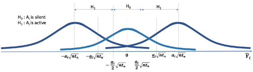
Figure 2: This figure shows how Bob makes his decision from $\bar{Y}_{i}$ for the random access case when they use the channel $n$ times. Here, Bob needs to output one of three outcomes, silent, $1$, and $0$. The right graph shows the distribution of $\bar{Y}_{i}$ when $M_{i}=0$, and the left graph shows the distribution of $\bar{Y}_{i}$ when $M_{i}=1$. The central graph shows the distribution of $\bar{Y}_{i}$ when ${\cal A}_{i}$ is silent.

Next, we consider Bob’s decoder. In order to recover $M_{i}$, using the secret variables $S_{i,j}$, Bob calculates the decision statistic $\bar{Y}_{i}:=\sum_{j=1}^{n}(-1)^{S_{i,j}}Y_{j}$ from his receiving variables $Y_{1},\ldots,Y_{n}$ as Fig. 2. For each $i$, Bob outputs one of three outcomes, silent, $1$, and $0$ as follows. When $|\bar{Y}_{i}|<\sqrt{n}\frac{\underline{a}t_{n}}{2}$, Bob considers that ${\cal A}_{i}$ is silent. When $\bar{Y}_{i}\leq-\sqrt{n}\frac{\underline{a}t_{n}}{2}$, Bob considers that $M_{i}$ is 1. When $\bar{Y}_{i}\geq\sqrt{n}\frac{\underline{a}t_{n}}{2}$, Bob considers that $M_{i}$ is 0.

Then, we have the following theorem for the analysis on the asymptotic performance of our code.

Theorem 1

Assume that the number of senders, $m$, and of active senders, $l$, and $m$, $l$ are given as $m_{n}$, $l_{n}=\frac{n}{t_{n}}$ to satisfy

$$\frac{n}{l_{n}^{2}} \to 0,$$ (4)

$$\frac{l_{n}}{n} \to 0,$$ (5)

$$\frac{n\underline{a}^{2}}{8l_{n}(v_{B}+\overline{a}^{2})}-\log m_{n} \to+\infty.$$ (6)

Also, we assume that $v_{W}$ belongs to an open set ${\cal V}$. Then, under the above presented protocol, Bob can recover the message with asymptotically zero error, and Willie cannot detect the existence of the communication regardless of the values of the channel parameter to Willie.

Here, we have not formulated Willie’s detection. In Section V-A, we state the impossibility of Willie’s detection after presenting its formal definition.

Interestingly, our encoder and our decoder do not depend on the values $a_{i},b_{i},v_{B},v_{W}$ of the channel parameters, and our decoder do not depend on the number $l_{n}$ of active senders. But, the probability of correct decoding depends on the number $l_{n}$, and is close to $1$ as long as the conditions (4) and (6) hold. Hence, in order that Bob knows whether his decoding is correct, he needs to know whether the number $l_{n}$ is smaller than a certain threshold, which can deduced by Bob from the estimated received power.

For example, when $l_{n}=cn\log n$ with $c<\frac{8(v_{B}+\overline{a}^{2})}{\underline{a}^{2}}$ and $m_{n}=O(n)$, the conditions (4) and (6) hold. Also, when $l_{n}=cn\log n$ with $c\leq\frac{8(v_{B}+\overline{a}^{2})}{\underline{a}^{2}}$ and $m_{n}=l_{n}$, these conditions hold. Therefore, covert communication with random access code is asymptotically possible with $O(n)$ senders and $O(n/\log n)$ active senders when all active senders transmit only one bit.

Now, we consider the case when each active sender ${\cal A}_{i}$ wants transmit $u_{n}=g(n)$ bits, $M_{i,1},\ldots,M_{i,u_{n}}$. In this case, the active sender ${\cal A}_{i}$ shares random binary symbols $S_{i,1,j},\ldots,S_{i,u_{n},j}$ with Bob for $j=1,\ldots,n$, and the active sender ${\cal A}_{i}$ sets $X_{i,j}$ as

$$X_{i,j}=\sqrt{\frac{t_{n}}{n}}\sum_{j^{\prime}=1}^{u_{n}}(-1)^{M_{i,j^{\prime}}+S_{i,j^{\prime},j}}$$ (7)

as the encoding. Here, we denote the numbers of senders and active senders by $m_{n}^{\prime}$ and $l_{n}^{\prime}$. This situation can be considered as a special case of Theorem 1 with $m_{n}=g(n)m_{n}^{\prime}$ and $l_{n}=g(n)l_{n}^{\prime}$. Hence, when $m_{n}=g(n)m_{n}^{\prime}$ and $l_{n}=g(n)l_{n}^{\prime}$ satisfy the conditions (4) and (6), Bob can recover the message with asymptotically zero error, and Willie cannot detect the existence of the communication regardless of the values of the channel parameter to Willie.

Also, the condition (6) implies that $t_{n}$ goes to zero. Since $t_{n}$ is the power per user, the power per user needs to be zero asymptotically in our protocol. This agrees with the intuition that covertness requires as low power as possible. Further, since the values of the channel parameter to Willie are not contained in the assumption of this theorem, the covert communication is possible even if Willie’s channel is better than Bob’s channel.

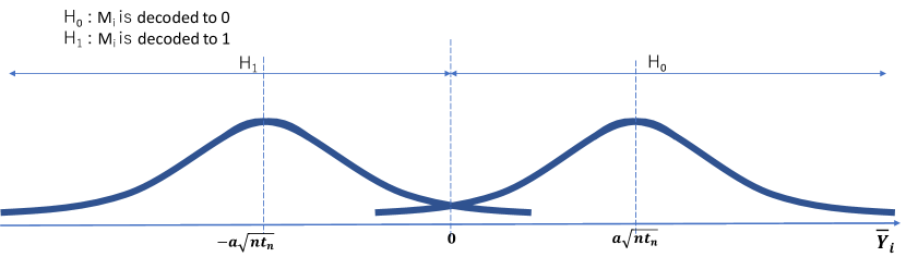
Figure 3: This figure shows how Bob decodes the message $M_{i}$ from $\bar{Y}_{i}$ for the point-to-point case. The right graph shows the distribution of $\bar{Y}_{i}$ when $M_{i}=0$, and the left graph shows the distribution of $\bar{Y}_{i}$ when $M_{i}=1$.

III Point-to-point channel

III-A Point-to-point channel model

In the following, we discuss what protocol is obtained when the above protocol is applied to the point-to-point channel model. In this model, the legitimate sender, Alice, intends to transmit $l_{n}$ bits to the legitimate receiver, Bob, with $n$ uses of AWGN channel while the intensity of input can be fixed to a single value intended by Alice during one block length. This setting is often called point-to-point communication. Table III summarizes the relation between random access channel and point-to-point channel.

TABLE III: Relation between random access channel and point-to-point channel

	random access	point-to-point
	channel	channel
$n$	number of uses of channel	block length
$l_{n}$	transmission length	transmission
	(number of active senders)	length
$m_{n}$	number of senders	this number is set to be $l_{n}$

When Alice’s $j$-th input variable is $X$, Bob receives

$$Y_{j}={N}_{B,j}+aX_{j}$$ (8)

for $j=1,\ldots,n$. The variables ${N}_{B,1},\ldots,N_{B,n}$ are independent Gaussian random variables with mean $0$ and variance $v_{B}$. Similarly, Willie receives

$$Z_{j}=N_{W,j}+bX_{j}$$ (9)

for $j=1,\ldots,n$. The variables ${N}_{W,1},\ldots,N_{W,n}$ are independent Gaussian random variables with mean $0$ and variance $v_{W}$. Then, we make the same assumption for $v_{B}$ and $v_{W}$ as the previous section. Here, when Alice is silent, all input variables $X_{1},\ldots,X_{n}$ are zero. Since $a$ and $b$ are the fading coefficients in Bob’s and Willie’s detection, $a$ and $b$ are positive constants during a coherent time. That is, we treat $a$ and $b$ as constants in the following discussion. Therefore, our model is the model in the previous section with $\underline{a}=\overline{a}=a$, $\underline{b}=\overline{b}=b$, and $m=l$.

III-B Covert protocol

For covert transmission of $l_{n}$ bits $M_{1},\ldots,M_{l_{n}}$ within the coherence channel time, Alice and Bob share $nl_{n}$ secret binary symbols $\{S_{i,j}\}_{1\leq j\leq n,1\leq i\leq l_{n}}$. Then, Alice encodes the message $M_{1},\ldots,M_{l_{n}}$ as

$$X_{j}=\sqrt{\frac{t_{n}}{n}}\sum_{i=1}^{l_{n}}(-1)^{M_{i}+S_{i,j}}$$ (10)

for $j=1,\ldots,n$. Here, the above code uses average power $\frac{t_{n}}{n}$ for each channel use, which is sufficiently small.

To see another form of $X_{j}$, we define $A_{j}$ as $A_{j}:=|\{i|M_{i}+S_{i,j}=1\hbox{ mod }2\}|$, where $|A|$ expresses the number of elements of the set $A$. Then, $A_{j}$ is independently subject to the binary distribution with $l$ trials and with probability $1/2$. $X_{j}$ has another form as

$$X_{j}=\sqrt{\frac{t_{n}}{n}}(l_{n}-2A_{j}).$$ (11)

The variable $\sqrt{\frac{t_{n}}{n}}(l_{n}-2A_{j})$ has average $0$ and variance $\frac{t_{n}l_{n}}{n}$. Hence, the power for one channel use, i.e., the expectation of $X_{j}^{2}$ is $\frac{t_{n}l_{n}}{n}$, which converges to zero.

Next, we consider Bob’s decoder. In order to recover $M_{i}$, using the secret variables $S_{i,j}$, Bob calculates the decision statistic $\bar{Y}_{i}:=\sum_{j=1}^{n}(-1)^{S_{i,j}}Y_{j}$ from his receiving variables $Y_{1},\ldots,Y_{n}$ as Fig. 3. When $\bar{Y}_{i}\leq 0$, Bob considers that $M_{i}$ is 1. When $\bar{Y}_{i}>0$, Bob considers that $M_{i}$ is 0. Then, we have the following theorem for the analysis on the asymptotic performance of our code. Hence, as a special case of Theorem 1, we have the following theorem.

Theorem 2

When $v_{W}$ belongs to an open set ${\cal V}$ and $l=l_{n}$ satisfies (4) and

$$\frac{n{a}^{2}}{8l_{n}(v_{B}+{a}^{2})}-\log l_{n} \to+\infty,$$ (12)

Bob can recover the message with asymptotically zero error, and Willie cannot detect the existence of the communication.

Similar to Theorem 1, we have not formulated Willie’s detection. In Section V-A, we state the impossibility of Willie’s detection after presenting its formal definition.

This theorem shows that covert communication is asymptotically possible with transmission length $cn\log n$ with $c\leq\frac{8(v_{B}+\overline{a}^{2})}{\underline{a}^{2}}$. Interestingly, our encoder and our decoder does not depend on the values $a,b,v_{B},v_{W}$ of the channel parameters as long as the condition (12) holds.

III-C Relation with redundant condition

The existing studies [4, 5] showed the following. When the channel to Willie satisfies the redundant condition, a better transmission rate. However, our channel model does satisfy this condition even when the channel parameters of the channel to Willie are fixed. Therefore, these existing results cannot be applied to our case. To see this fact, we recall the definition of the redundant condition.

We denote the output sample space in the channel to Willie by ${\cal Z}$, which is potentially an infinite set. We also denote a measure on ${\cal Z}$ by $\nu(dz)$. We denote the set of Alice’s input by ${\cal X}$, which is a finite set. Depending on Alice’s input $x\in{\cal X}$, Willie’s output is subject to the probability density function $p_{Z,x}$. When the following condition holds, the channel to Willie is called redundant. There exist two non-identical distributions $P_{X}$ and $P_{X}^{\prime}$ such that

$$\sum_{x\in{\cal X}}P_{X}(x)p_{Z,x}=\sum_{x\in{\cal X}}P_{X}^{\prime}(x)p_{Z,x}.$$ (13)

In our model (9), the Willie’s output is simplified as

$$Z=N_{W}+bX.$$ (14)

Here, the variable ${N}_{W}$ is a Gaussian random variables with mean $0$ and variance $v_{W}$. Since our channel model of the channel to Willie does not satisfy the redundant condition with given $v_{W}$ and $b$, we cannot directly apply the existing method by [4, 5] to our model.

III-D Comparison with existing methods

Many recent researchers [15, 16, 17, 18, 19, 20, 21, 22] have obtained achievability of covert transmission of $O(n)$ bits when only Willie’s channel has uncertainty and Bob knows a certain knowledge of his own channel unlike our assumption. When the fading coefficient $a$ is known and only the noise power $v_{B}$ is unknown, the decoder for the case with the maximum noise power works well. Hence, the existing method does work well in this case. For example, the paper [17] assumes that the fading coefficient $a$ is 1 while $v_{B}$ is unknown. However, when the fading coefficient $a$ is unknown in addition to $v_{B}$, the conventional decoder does not work because the decoder depends on the value of the fading coefficient $a$. To understand this difficulty, consider the following case with $n=1$. The sender uses four points $\pm x_{1}$ and $\pm x_{0}$ in $\mathbb{R}$ with $x_{1}>x_{0}>0$ for the encoding. When the receiver receives a value $y\in(x_{0},x_{1})\subset\mathbb{R}$, the maximum likelihood (ML) decoder depends on the value of the fading coefficient $a$. When $a<\frac{2y}{x_{1}-x_{0}}$, the ML decoder estimates that the input is $+x_{1}$. Otherwise, it estimates that the input is $+x_{0}$. In this way, the decoder depends on the value of the fading coefficient $a$ in general. In the case of conventional channel coding, people often employ universal coding to resolve this problem. The method of type [30] enables us to develop universal coding for the discrete memoryless channel case. The paper [31] proposed a universal coding that works for the continuous case including the AWGN channels. In this way, it is a crucial technology to develop a code that works independently of the channel parameters.

To see the difficulty to achieve the covert transmission under imperfect knowledge for both channels, the following part discusses what problem appears in simple applications of the original methods [5, 4] under our setting. Our channel model has a uncertainty for the variance $v_{W}$ of the additive Gaussian noise in the channel to the adversary. This situation is formulated as follows. Users know that the variance of the additive Gaussian noise in the channel to the adversary, Willie, belongs to an open set ${\cal V}$, but they cannot identify which value in ${\cal V}$ is the true value $v_{W}$.

Since Alice is allowed to use various values as the channel input power in the Gaussian point-to-point channel, Alice can select the input $X_{j}$ freely. Hence, we can apply the method [5] for the redundant case as follows. First we choose a sufficiently small positive number $v^{\prime}$ such that $v_{W}+b^{2}v^{\prime}$ belongs to ${\cal V}$. Here, $v^{\prime}$ expresses the possible error for Willie’s knowledge about the variance of the additive Gaussian noise in the channel to Willie. That is, even when the true value is $v_{W}$, Willie cannot identify which of $v_{W}$ and $v_{W}+b^{2}v^{\prime}$ is the true. Hence, Willie has to keep the possibility that $v_{W}+b^{2}v^{\prime}$ is the true as well as $v_{W}$.

Let $R_{v^{\prime}}$ be a real number such that $R_{v^{\prime}}<I(Y_{j};X_{j})$, where $X_{j}$ is subject to the Gaussian distribution with variance $v^{\prime}$ and mean $0$. Using the conventional random coding of rate $R_{v^{\prime}}$ with respect to the above Gaussian distribution, we generate a code. Here, the choice of the code is a part of the preshared information between Alice and Bob. When Alice encodes the message $M_{n}$ via the preshared code, using the preshared code, Bob decodes message $M_{n}$. However, as is discussed in the paper [5], in this case, Willie cannot distinguish the received signals from the Gaussian distribution with variance $v_{W}+b^{2}v^{\prime}$ and mean $0$, which is a special case of the silent case. In this way, this method achieves the covert transmission of $O(n)$ bits. Although this method has a higher covert transmission speed than our method, it has the following problem. When the decoder of this method is a maximum likelihood decoder, it depends on the value of $a$ while it does not depend on the value of $v_{W}$. That is, the above method satisfies the condition (i), but does not satisfy the condition (ii);

(i)

Willie’s output of the code simulates the Gaussian distribution with variance $v_{W}+b^{2}v^{\prime}$ and mean $0$.

(ii)

Bob’s decoder does not depend on the channel parameters $a$ and $v_{B}$.

Although the paper [31] proposed a universal coding that works for the AWGN channel, the encoder of [31] is generated by a distribution with finite support. Hence, use of the method [31] satisfies the condition (ii), but does not satisfy the condition (i).

As another idea, we apply the method [4] as follows. The method [4] employs the code for wire-tap channel. Since the paper [39, Appendix D] proposed a wire-tap code for the AWGN channels, the method [4] satisfies the condition (i) when Bob knows the channel parameters of the channel to Bob. That is, this alternative method does not satisfy the condition (ii). Fortunately, our code satisfies both conditions, i.e., our method is the first method to achieve both conditions (i) and (ii). In this sense, our code has an advantage over a simple application of the methods [4, 5].

IV Analysis of Bob’s decoding

IV-A Characterization of correct decoding

The aim of this section is the asymptotic evaluation of the probability that Bob correctly decodes all messages including the detection of the existence of communication from all senders. In this subsection, we derive a lower bound of this probability.

Bob’s receiving signal is written as

$$Y_{j}=N_{B,j}+\sqrt{\frac{t_{n}}{n}}\sum_{k=1}^{l_{n}}a_{i_{k}}(-1)^{M_{i_{k}}+S_{i_{k},j}}.$$ (15)

The variable $\bar{N}_{B,i}:=\sum_{j=1}^{n}(-1)^{S_{i,j}}{N}_{B,j}$ is a Gaussian variable with average $0$ and variance $nv_{B}$. The variables $M_{i_{k}}+S_{i_{k},j}+S_{i,j}$ with $j=1,\ldots,n$ and $k=1,\ldots,l_{n}$ with $i_{k}\neq i$ are independent binary random variables subject to the uniform distribution.

When Bob focuses on $\bar{Y}_{i}$ to recover $M_{i}$, only the term related to $M_{i}$ is of his interest and the remaining terms can be considered as noises. Hence, by using $N(i):=\bar{N}_{B,i}+\sqrt{\frac{t_{n}}{n}}\sum_{k=1,i_{k}\neq i}^{l_{n}}a_{i_{k}}\sum_{j=1}^{n}(-1)^{M_{i_{k}}+S_{i_{k},j}+S_{i,j}}$, the term $\bar{Y}_{i}$ can be rewritten as

$$\bar{Y}_{i}=\sum_{j=1}^{n}(-1)^{S_{i,j}}Y_{j}$$

$$= \sum_{j=1}^{n}(-1)^{S_{i,j}}\Big{(}{N}_{j}+\sqrt{\frac{t_{n}}{n}}\sum_{k=1}^{l}a_{i_{k}}(-1)^{M_{i_{k}}+S_{i_{k},j}}\Big{)}$$

$$= \bar{N}_{B,i}+\sqrt{\frac{t_{n}}{n}}\sum_{k=1}^{l_{n}}a_{i_{k}}\sum_{j=1}^{n}(-1)^{M_{i_{k}}+S_{i_{k},j}+S_{i,j}}$$

$$= \bar{N}_{B,i}+\sqrt{nt_{n}}a_{i}(-1)^{M_{i}}+\sqrt{\frac{t_{n}}{n}}\sum_{k=1,i_{k}\neq i}^{l_{n}}a_{i_{k}}\sum_{j=1}^{n}(-1)^{M_{i_{k}}+S_{i_{k},j}+S_{i,j}}$$

$$= \sqrt{nt_{n}}a_{i}(-1)^{M_{i}}+{N}(i).$$ (16)

That is, $N(i)$ is considered as a noise.

Assume that ${\cal A}_{i}$ is silent, i.e., $i\in(\{i_{k}\}_{k=1}^{l_{n}})^{c}$. Bob’s decoding is correct when $|N(i)|<\sqrt{nt_{n}}\frac{\underline{a}}{2}$. That is, the probability of Bob’s correct decoding is ${\rm Pr}\Big{(}|N(i)|<\sqrt{nt_{n}}\frac{\underline{a}}{2}\Big{)}$. See Fig. 2 to illustrate this process.

Assume that ${\cal A}_{i}$ is active. Bob’s decoding is correct when $M_{i}=0$ and $N(i)\leq\sqrt{nt_{n}}(a_{i}-\frac{\underline{a}}{2})$. Also, Bob’s decoding is correct when $M_{i}=1$ and $N(i)\geq-\sqrt{nt_{n}}(a_{i}-\frac{\underline{a}}{2})$. Since $N(i)$ is symmetric, i.e., the distribution of $N(i)$ is the same as the distribution of $-N(i)$, the probability of Bob’s correct decoding is ${\rm Pr}\Big{(}N(i)\leq\sqrt{nt_{n}}(a_{i}-\frac{\underline{a}}{2})\Big{)}$.

Then, we obtain the following lower bound for the probability that Bob correctly decodes all messages including the detection of the existence of communication from all senders.

$$P_{n}:= \prod_{k=1}^{l_{n}}{\rm Pr}\Big{(}N(i_{k})\leq\sqrt{nt_{n}}(a_{i_{k}}-\frac{\underline{a}}{2})\Big{)}$$

$$\cdot\prod_{i\in(\{i_{k}\}_{k=1}^{l_{n}})^{c}}{\rm Pr}\Big{(}|N(i)|<\sqrt{nt_{n}}\frac{\underline{a}}{2}\Big{)}.$$ (17)

Then, as shown in Appendix A, we have the following lemma.

Lemma 1

When $l$ is given as $l_{n}=\frac{n}{t_{n}}$ and the conditions (4) and (6) hold, we have

$$P_{n}\to 1,$$ (18)

Since the probability $P_{n}$ is a non-negative value upper bounded by $1$, its convergence speed to 1 is evaluated by the speed of the convergence of $\log P_{n}$ to $0$. That is, this convergence is evaluated by the speed of the convergence of $\log(-\log P_{n})$ to $-\infty$. The following expresses an upper bound of this convergence speed.

$$\log(-\log P_{n})\leq-\frac{n\underline{a}^{2}}{8l_{n}(v_{B}+\overline{a}^{2})}+\log m_{n}+\log 2+o(1).$$ (19)

The condition (6) guarantees that this lower bound goes to $-\infty$.

IV-B Single sender case

The single sender case can be evaluated by putting $\underline{a}=\overline{a}=a$ and $m_{n}=l_{n}$. In the same way as (16), we have

$$\bar{Y}_{i}=\sqrt{nt_{n}}a(-1)^{M_{i}}+{N}(i),$$ (20)

where

$${N}(i):=\bar{N}_{i}+a\sqrt{\frac{t_{n}}{n}}\sum_{i^{\prime}=1,i\neq i}^{l_{n}}\sum_{j=1}^{n}(-1)^{M_{i^{\prime}}+S_{i^{\prime},j}+S_{i,j}}.$$ (21)

Since ${N}(i)$ is symmetric, in the same way as (17), the probability of correct decoding is lower bounded as

$$\prod_{k=1}^{l_{n}}{\rm Pr}\Big{(}N(i)<\sqrt{nt_{n}}a\Big{)}.$$ (22)

Then, as a special case of Lemma 1, we have the following lemma.

Lemma 2

When $l$ is given as $l_{n}=\frac{n}{t_{n}}$ and the conditions (4) and (12) hold, we have

$$\prod_{k=1}^{l_{n}}{\rm Pr}\Big{(}N(i)<\sqrt{nt_{n}}a\Big{)}\to 1.$$ (23)

V Willie’s detection

V-A Formulation

Since the random access channel model contains the point-to-point channel as a special case with $\underline{b}=\overline{b}=b$ and $m_{n}=l_{n}$, we discuss the random access channel model in the following. Under the encoder (3), Willie’s receiving signal is written as

$$Z_{j}=N_{W,j}+\frac{1}{\sqrt{n}}\sum_{k=1}^{l_{n}}b_{i_{k}}(-1)^{M_{i_{k}}+S_{i_{k},j}}.$$ (24)

We denote the distribution for $Z_{j}$ by $P_{Z_{j}}$ and denote the joint distribution for $Z=(Z_{1},\ldots,Z_{n})$ by $P_{Z}$. $P_{Z|M=m}$ expresses the conditional distribution under the condition $M(:=(M_{1},\ldots,M_{l_{n}}))=m(:=(m_{1},\ldots,m_{l_{n}}))$.

We denote the Gaussian distribution with average $0$ and variance $v$ by $G_{v}$. When all senders are silent, Willie’s observation $(Z_{1},\ldots,Z_{n})$ is subject to the distribution $G_{v_{W}}^{n}$. Also, we assume that Willie does not know the exact value of the variance $v_{W}$ of his receiving device while Willie knows its rough value because a part of the noise $N_{W,j}$ is generated out of Willie’s device, which can be considered as a background noise. Then, we denote the set of possible variances with the silent case by ${\cal V}$. In the following, we assume that ${\cal V}$ is an open set of $\mathbb{R}$.

In this case, to cover Willie’s advantageous scenario, we assume that Willie knows the secret message $M$, but he does not know the binary symbols $\{S_{i,j}\}$. That is, we show that Willie cannot detect the existence of the communication even though he knows the secret message $M$. When no communication is made, the joint distribution of Willie’ receiving signal $Z$ and the secret message belongs to the set $\{G_{v_{W}}^{n}\times P_{M}|v_{W}\in{\cal V}\}$.

It is known that the statistical distinguishablity is characterized by the variational distance as follows, where we denote the variational distance between $P$ and $Q$ by $d_{V}(P,Q)$. Given a method ${\cal T}$ to distinguish $P$ and $Q$, we denote the probability being incorrectly deciding the distribution to be $P$ while the true is $Q$, by $\epsilon_{1}({\cal T})$, and the probability being incorrectly deciding the distribution to be $Q$ while the true is $P$, by $\epsilon_{2}({\cal T})$. The sum of $\epsilon_{1}({\cal T})$ and $\epsilon_{2}({\cal T})$ is evaluated as .

$$\epsilon_{1}({\cal T})+\epsilon_{2}({\cal T})\geq 1-d_{V}(P,Q).$$ (25)

Hence, the distinguishability between the real distribution $P_{Z,M}$ of making the communication and the case with no communication is measured by the minimum $\min_{{v}\in{\cal V}}d_{V}(P_{Z,M},G_{{v}}^{n}\times P_{M})$, which shows the ability of distinguishing the following two hypotheses. One is the hypothesis that the true distribution is $P_{Z,M}$, which corresponds to the case of making the communication. The other one is the hypothesis that the true distribution belongs to the set $\{G_{v_{W}}^{n}\times P_{M}|v_{W}\in{\cal V}\}$, which corresponds to the case of no communication. Hence, when our covertness measure $\min_{{v}\in{\cal V}}d_{V}(P_{Z,M},G_{{v}}^{n}\times P_{M})$ is sufficiently small with any $l$ active senders, the situation with any $l$ active senders cannot be distinguished with the situation with no communication, i.e., Willie cannot detect any active user.

Theorem 3

Assume that $l$ is given as $l_{n}=\frac{n}{t_{n}}$ to satisfy the condition (5). Also, we assume that $v_{W}$ belongs to ${\cal V}$, Then, our covertness measure goes to zero as under the protocol presented in Section II-B

$$\min_{{v}\in{\cal V}}d_{V}(P_{Z,M},G_{{v}}^{n}\times P_{M})\to 0.$$ (26)

The combination of Lemma 1 and Theorem 3 leads Theorem 1.

Further, under the case with equal fading in Willie’s detection, the condition in Theorem 3 can be relaxed as follows.

Theorem 4

Assume that $\underline{b}=\overline{b}=b$ and $l$ is given as $l_{n}=\frac{n}{t_{n}}$ to satisfy the condition

$$\frac{n}{l_{n}^{2}},\frac{l_{n}^{2}}{n^{3}} \to 0.$$ (27)

Also, we assume that $v_{W}$ belongs to ${\cal V}$, Then, our covertness measure goes to zero under the protocol presented in Section II-B as

$$\min_{{v}\in{\cal V}}d_{V}(P_{Z,M},G_{{v}}^{n}\times P_{M})\to 0.$$ (28)

When $l_{n}$ is linear with $n$, the condition (5) does not hold, but the condition (27) does hold. In this sense, Theorem 4 has a weaker condition for $l_{n}$ than Theorem 3. The case with equal fading in Willie’s detection, i.e., the case with $\underline{b}=\overline{b}=b$, covers the case with the point-to-point channel. Thus, due to Theorem 4, one sender, Alice, can send $l_{n}$ bits to Bob in one channel coherence time securely with covertness to Willie. the conditions (4) and (6) imply the condition (27), the combination of Lemma 2 and Theorem 4 leads Theorem 2.

V-B Useful formula for our covertness measure

As a preparation of our proofs of Theorems 3 and 4, we prepare a useful formula for our covertness measure, i.e., the minimum variational distance as follows.

$$\min_{{v}\in{\cal V}}d_{V}(P_{Z,M},G_{{v}}^{n}\times P_{M})$$

$$\leq \min_{{v}\in{\cal V}}d_{V}(D(P_{Z,M},P_{Z}\times P_{M})+d_{V}(P_{Z}\times P_{M},G_{{v}}^{n}\times P_{M})$$

$$= d_{V}(P_{Z,M},P_{Z}\times P_{M})+\min_{{v}\in{\cal V}}d_{V}(P_{Z},G_{{v}}^{n}).$$ (29)

The first term $d_{V}(P_{Z,M},P_{Z}\times P_{M})$ expresses the secrecy of the message, and the second term $\min_{{v}\in{\cal V}}d_{V}(P_{Z},G_{{v}}^{n})$ expresses the possibility that Willie detects the existence of the communication.

The variables $(M_{i}+S_{i_{k},j})_{k,j}$ are independently subject to the binary uniform distribution under the condition $M=m$. The variables $Z=(Z_{1},\ldots,Z_{n})$ do not depend on $m$. That is, we have $P_{Z|M=m}=P_{Z}$. Hence, Willie has no information for the message $M=m$, i.e.,

$$d_{V}(P_{Z,M},P_{Z}\times P_{M})=0.$$ (30)

In the following, we discuss $\min_{{v}\in{\cal V}}d_{V}(P_{Z},G_{{v}}^{n})$. We choose $v^{\prime}:=\frac{1}{n}\sum_{k=1}^{l}b_{i_{k}}^{2}$. When $c=\frac{l}{n}$ is sufficiently small, $v^{\prime}$ is small so that $v_{W}+v^{\prime}$ belongs to ${\cal V}$ because $v_{W}\in{\cal V}$ and ${\cal V}$ is an open set. Hence, we have

$$\min_{v\in{\cal V}}d_{V}(P_{Z},G_{v}^{n})\leq d_{V}(P_{Z},G_{v_{W}+v^{\prime}}^{n}).$$ (31)

Combining (29), (30), and (31), we obtain

$$\min_{{v}\in{\cal V}}d_{V}(P_{Z,M},G_{{v}}^{n}\times P_{M})\leq d_{V}(P_{Z},G_{v_{W}+v^{\prime}}^{n}).$$ (32)

Applying the Pinsker inequality $d_{V}(P,Q)^{2}\leq\frac{1}{2}D(P\|Q)$, where $D(P\|Q):=\int(\log P(x)-\log Q(x))P(x)dx$, we have $d_{V}(P_{Z},G_{v_{W}+v^{\prime}}^{n})^{2}\leq\frac{1}{2}D(P_{Z_{1},\ldots,Z_{n}}\|G_{v_{E}+v^{\prime}}^{n})$. Hence, it is sufficient to show that the relative entropy $D(P_{Z_{1},\ldots,Z_{n}}\|G_{v_{E}+v^{\prime}}^{n})$ between the joint distribution $P_{Z_{1},\ldots,Z_{n}}$ of the random variables $Z_{1},\ldots,Z_{n}$ and the $n$-fold Gaussian distribution $G_{v_{E}+v^{\prime}}^{n}$ is sufficiently small. Combining (29), (30), and the above application of the Pinsker inequality, we have

$$\min_{{v}\in{\cal V}}d_{V}(P_{Z,M},G_{{v}}^{n}\times P_{M})\leq\sqrt{\frac{1}{2}D(P_{Z_{1},\ldots,Z_{n}}\|G_{v_{E}+v^{\prime}}^{n})}.$$ (33)

Therefore, the remaining part evaluates $D(P_{Z_{1},\ldots,Z_{n}}\|G_{v_{E}+v^{\prime}}^{n})$.

V-C Analysis of case with equal fading

Now, we show Theorem 4 by using the result in [33]. We assume that $\underline{b}=\overline{b}=b$. To state the result by [33], we define $\chi^{2}$ distance $\chi^{2}(P,Q)$ as

$$\chi^{2}(P,Q):=\int\frac{(p(x)-q(x))^{2}}{q(x)}dx,$$ (34)

where $p$ and $q$ are probability density functions of the distributions $P$ and $Q$. We define Renyi divergence of order $2$, $D_{2}(P\|Q)$ as

$$D_{2}(P\|Q):=\log\int\frac{p(x)^{2}}{q(x)}dx.$$ (35)

We have

$$D(P\|Q)\leq D_{2}(P\|Q)\leq\log(1+\chi^{2}(P,Q))\leq\chi^{2}(P,Q).$$ (36)

Proposition 1 ([33, (1.3)])

$U_{1},\ldots,U_{n}$ are $n$ independent and identical distributed variables with average $0$ and variance $v_{W}$. The distribution of $U_{i}$ is absolutely continuous and has the probability density function $P_{U}(u)$. $P_{U}(u)$ is symmetric, i.e., $P_{U}(u)=P_{U}(-u)$. Define

$${\cal U}_{n}:=\sum_{i=1}^{n}\frac{1}{\sqrt{n}}U_{i}.$$ (37)

Then, we have

$$\chi^{2}(P_{{\cal U}_{n}},G_{1})=\frac{(\alpha_{4}-3)^{2}}{24n^{2}}+O(\frac{1}{n^{3}}),$$ (38)

where $\alpha_{4}:=\mathbb{E}[G_{1}^{4}]$.

Since $v^{\prime}$ is simplified as $v^{\prime}=\frac{l_{n}b^{2}}{n}=\frac{b^{2}}{t_{n}}$, we have

$$\alpha_{4}(j):=\mathbb{E}\Big{[}\Big{(}\frac{1}{\sqrt{v+v^{\prime}}}Z_{j}\Big{)}^{4}\Big{]}=\frac{{v^{\prime}}^{2}+6v_{W}v^{\prime}+3v^{2}}{(v_{W}+v^{\prime})^{2}}$$

$$= \frac{{v^{\prime}}^{2}+6v_{W}v^{\prime}+3v^{2}-3(v_{W}+v^{\prime})^{2}}{(v_{W}+v^{\prime})^{2}}+3=\frac{-2(\frac{b^{2}}{t_{n}})^{2}}{(v_{W}+\frac{b^{2}}{t_{n}})^{2}}+3.$$ (39)

Since $\underline{b}=\overline{b}=b$, we have $b_{i_{k}}=b$ for all $k$, Proposition 1 guarantees that

$$\chi^{2}(P_{Z_{j}},G_{v_{W}+v^{\prime}})=\chi^{2}(P_{\frac{1}{\sqrt{v+v^{\prime}}}Z_{j}},G_{1})$$

$$= \frac{\big{(}\alpha_{4}(j)-3\big{)}^{2}}{24l^{2}}+O(\frac{1}{l_{n}^{3}})$$

$$\stackrel{{\scriptstyle(a)}}{{=}} \frac{4(\frac{b^{2}}{t_{n}})^{4}}{24l_{n}^{2}(v_{W}+\frac{b^{2}}{t_{n}})^{4}}+O(\frac{1}{l_{n}^{3}})=\frac{b^{8}}{6n^{2}t_{n}^{2}(v_{W}+b^{2}t_{n}^{-1})^{4}}+O(\frac{t_{n}^{3}}{n^{3}}),$$ (40)

where $(a)$ follows from (39). Hence, we have

$$D(P_{Z_{j}}\|G_{v_{W}+v^{\prime}})\leq\frac{b^{8}}{6n^{2}t_{n}^{2}(v_{W}+b^{2}t_{n}^{-1})^{4}}+O(\frac{t_{n}^{3}}{n^{3}}).$$ (41)

Thus,

$$D(P_{Z_{1},\ldots,Z_{n}}\|G_{v_{W}+v^{\prime}}^{n})\leq n\Big{(}\frac{b^{8}}{6n^{2}t_{n}^{2}(v_{W}+b^{2}t_{n}^{-1})^{4}}+O(\frac{t_{n}^{3}}{n^{3}})\Big{)}$$

$$= \frac{b^{8}}{6nt_{n}^{2}(v_{W}+b^{2}t_{n}^{-1})^{4}}+O(\frac{t_{n}^{3}}{n^{2}}).$$ (42)

The condition (27) guarantees that $\frac{b^{8}}{6nt_{n}^{2}(v_{W}+b^{2}t_{n}^{-1})^{4}}$ and $\frac{t_{n}^{3}}{n^{2}}$ go to zero, which implies that the term $D(P_{Z_{1},\ldots,Z_{n}}\|G_{v_{W}+v^{\prime}}^{n})$ goes to zero. Hence, combining (33), we obtain Theorem 4.

V-D Analysis of case with unequal fading

Now, we show Theorem 3. We consider the case with unequal fading in Willie’s detection. For the analysis of this case, we have the following theorem.

Theorem 5

The relative entropy $D(P_{Z_{1},\ldots,Z_{n}}\|G_{v_{W}+v^{\prime}}^{n})$ is evaluated as

$$D(P_{Z_{1},\ldots,Z_{n}}\|G_{v_{W}+v^{\prime}}^{n})$$

$$\leq \frac{\frac{1}{n{v^{\prime}}^{2}}\sum_{k=1}^{l_{n}}b_{i_{k}}^{4}\Big{(}\frac{(v_{W}+v^{\prime})(e^{\frac{v^{\prime}}{v_{W}+2v^{\prime}}}+e^{-\frac{v^{\prime}}{v_{W}}})}{2\sqrt{v_{W}(v_{W}+2v^{\prime})}}-1\Big{)}}{\frac{e^{-\frac{v^{\prime}+v_{W}}{2v_{W}}}}{2}+(1-\frac{e^{-\frac{v^{\prime}+v_{W}}{2v_{W}}}}{2})\frac{1}{n^{2}{v^{\prime}}^{2}}\sum_{k=1}^{l_{n}}b_{i_{k}}^{4}}.$$ (43)

Since the proof of this theorem is very long, Appendix C proves it by using the result in [35], which employs the Poincaré constant.

We choose $c_{n}:=\frac{l_{n}}{n}=\frac{1}{t_{n}}$. We have $\sum_{k=1}^{l_{n}}b_{i_{k}}^{4}\leq{l_{n}}\overline{b}^{4}=c_{n}\overline{b}^{4}n$ and $v^{\prime}\leq\frac{l_{n}\overline{b}^{2}}{n}=c_{n}\overline{b}^{2}$. Since the condition (5) by using (66), the RHS of (43) is evaluated as

$$(\hbox{ RHS of }\eqref{NM})$$

$$\leq \frac{\sum_{k=1}^{l_{n}}b_{i_{k}}^{4}}{n{v^{\prime}}^{2}}\frac{1}{\frac{e^{-\frac{v^{\prime}+v_{W}}{2v_{W}}}}{2}}\Big{(}\frac{1}{6}\Big{(}\frac{v^{\prime}}{v_{W}}\Big{)}^{3}+O\Big{(}\Big{(}\frac{v^{\prime}}{v_{W}}\Big{)}^{4}\Big{)}\Big{)}$$

$$= \Big{(}\sum_{k=1}^{l_{n}}b_{i_{k}}^{4}\Big{)}\frac{e^{1/2}}{3}\Big{(}\frac{v^{\prime}}{nv_{W}^{3}}\Big{)}\Big{(}1+O\Big{(}\frac{v^{\prime}}{v_{W}}\Big{)}\Big{)}+O\Big{(}\Big{(}\frac{v^{\prime}}{v_{W}}\Big{)}^{4}\Big{)}$$

$$\leq c_{n}\overline{b}^{4}\frac{e^{1/2}}{3}\Big{(}\frac{c\overline{b}^{2}}{v_{W}^{3}}\Big{)}(1+O(c_{n}))+O(c_{n}^{4})$$

$$= \frac{c_{n}^{2}e^{1/2}}{3}\Big{(}\frac{\overline{b}^{2}}{v_{W}}\Big{)}^{3}+O(c_{n}^{3}).$$ (44)

Since the condition (5) guarantee that $c_{n}\to 0$, we have

$$D(P_{Z_{1},\ldots,Z_{n}}\|G_{v_{W}+v^{\prime}}^{n})\to 0.$$ (45)

Hence, combining (33), we complete the proof of Theorem 3.

Here, we compare the evaluation of (43) with the evaluation of (42). Eq. (43) has the order $O(\frac{1}{t_{n}^{2}})=O(\frac{1}{\log n^{2}})$ for $n$, and Eq. (42) has the order $O(\frac{1}{nt_{n}^{2}})=O(\frac{1}{n\log n^{2}})$ for $n$. Hence, Eq. (42) results in a much better covertness evaluation than Eq. (43). Therefore, combining this discussion and Lemma 1, we obtain Theorem 1.

VI Discussion and open problems

We have discussed covert communication assuming BPSK over AWGN channels. Our results are composed of two contributions: covert communications for the random access channel and point-to-point communication. In the former case, we assume that the sender can choose the power to a certain value that is fixed during a coding block length. Our encoder and our decoder in both settings are quite simple. Thus, the proposed methods are easily implementable being the main complexity the problem of key sharing, as in traditional spread spectrum. However, we have not described the detail of the implementation of our method based on spread-spectrum principle, which is needed for practical application. Its detailed description is an important future study.

In our method, we assume that Willie does not have perfect knowledge on the channel parameter. That is, using this lack of Willie’s knowledge, our method improves the transmission speed over existing methods [11, 12, 13] in the case of AWGN channel. The key idea for our method is convergence of the distribution of the weighted sample mean of $n$ independent random variables to a Gaussian distribution, which is related to a kind of central limit theorem [32]. This method depends on the fact that our output distribution is a Gaussian distribution. That is, it is impossible to extend this method to another channel model. Due to this reason, we also assume that Bob does not have perfect knowledge on the channel parameter. Our code is shown to guarantee that Bob reliably recovers the message under this condition. That is, our code is a universal code in this sense unlike the recent papers [15, 16, 17, 18, 19, 20, 21, 22].

In addition, since our covertness analysis needs the evaluation of the variational distance, we need more precise evaluation than the variant of central limit theorem [32]. To resolve this problem, we have employed the results from the papers [33, 35, 34]. As discussed in Section V-C, the result in [33] has been used for the analysis on the case with equal fading. For the general case with unequal fading, as discussed in Section V-D, the analysis on the papers [35, 34] employs Poincaré constant [36, 37, 34, 35]. Although Section V-D analyzes the case with unequal fading, the evaluation in Section V-C is tighter than in Section V-D. Hence, the above analysis has better evaluation for the ability of Willie’s detection of the existence of the communication than the use of evaluation in Section V-D. Hence, Eq. (42) suggests a possibility to improve the evaluation (43). For this improvement, it is needed to extend Proposition 1 to the case (62), i.e., the case with unequal weighted sum. It is an interesting a future study.

Further, we have not proved the converse part for the transmission length for our covert communication model. Since our code construction is based on an elementary idea, there is a possibility to improve the transmission speed of our method. It is another future problem to derive the asymptotically tight transmission speed under both settings. In the relation to this topic, to state the advantage of our method for the point-to-point communication, we have pointed that existing methods [4, 5] need perfect knowledge for channel parameters. That is, our model requires a code to satisfy the two conditions (i) and (ii) defined in Section III-D simultaneously. Although our code satisfies both conditions, we have not shown that no code with transmission length $O(n)$ satisfies both conditions in the point-to-point communication. In fact, in our protocol for the point-to-point communication, our code is essentially constructed with bit-by-bit communication. Clearly, this method is not efficient when covertness is not discussed. Therefore, it is an interesting point whether or not our protocol can be improved by a more efficient method in the point-to-point scenario. It is another open problem to clarify this issue.

Also, our method needs pre-shared secret of $O(n^{2})$ bits. Since this is larger than the size of transmitted message, it is better to reduce this size while keeping our transmission rate. One possibility for this solution is choosing the matrix $S_{i,j}$ to be a Toeplitz matrix. While this choice reduces the size of pre-shared secret to $O(n)$, it changes the stochastic behaviors of $Y_{j}$ and $Z_{j}$. It is another future study to evaluate the performance of this modified code. Finally, it is an interesting future study to apply the theoretical limits obtained in this work to a practical engineering setting with realistic fading channel parameters and evaluate the performance with practical BPSK symbol acquisition and realistic channel dynamics using metrics such as covert security outage probability.

Appendix A Proof of Lemma 1

To evaluate the above quantity, we introduce two kinds of cummulant generating functions $\phi_{b}$ and $\phi_{g,v}$ as

$$\phi_{b}(s):=\log\frac{e^{s}+e^{-s}}{2},\quad\phi_{g,v}:=\frac{vs^{2}}{2}.$$ (46)

That is, $\phi_{b}$ is the cummulant generating function of the variable $(-1)^{X}$ when $X$ obeys the binary distribution with probability $\frac{1}{2}$, and $\phi_{g,v}$ is the cummulant generating function of Gaussian distribution with average 0 and variance $v$. Therefore, the cummulant generating function of $N(i)$ is $\phi_{n,i}(s):=\phi_{g,nv_{B}}(s)+\sum_{k=1,i_{k}\neq i}^{l_{n}}n\phi_{b}(a_{i_{k}}s\sqrt{\frac{t_{n}}{n}})$. We have

$$\phi_{n,i}(s)\leq\phi_{n}(s):=\phi_{g,nv_{B}}(s)+l_{n}n\phi_{b}\Big{(}\overline{a}s\sqrt{\frac{t_{n}}{n}}\Big{)}.$$ (47)

When $n$ is large,

$$\phi_{n}(s) =\frac{s^{2}}{2}(nv_{B}+l_{n}\overline{a}^{2}t_{n})+O\Big{(}nl\Big{(}\frac{t_{n}}{n}\Big{)}^{\frac{3}{2}}s^{3}\Big{)}$$

$$=\frac{s^{2}}{2}(nv_{B}+l_{n}\overline{a}^{2}t_{n})+O\Big{(}l\sqrt{\frac{t_{n}^{3}}{n}}s^{3}\Big{)}.$$ (48)

We assume that ${\cal A}_{i}$ is silent. Since the condition (4) guarantees $\frac{n}{l_{n}^{2}}\to 0$, using (48), we have

$$\beta_{n}:= \max_{s}\Big{(}s\sqrt{nt_{n}}\frac{\underline{a}}{2}-\phi_{n}(s)\Big{)}$$

$$= \frac{(\sqrt{nt_{n}}\frac{\underline{a}}{2})^{2}}{2(nv_{B}+l_{n}\overline{a}^{2}t_{n})}+O\Big{(}l_{n}\sqrt{\frac{t_{n}^{3}}{n}}(\frac{\sqrt{t_{n}}}{\sqrt{n}v_{B}})^{3}\Big{)}$$

$$= \frac{nt_{n}\underline{a}^{2}}{8n(v_{B}+\overline{a}^{2})}+O\Big{(}\frac{l_{n}t_{n}^{3}}{n^{2}v_{B}^{3}}\Big{)}=\frac{t_{n}\underline{a}^{2}}{8(v_{B}+\overline{a}^{2})}+o(1).$$ (49)

Thus, under the condition (6), we have

$$m_{n}\exp(-\beta_{n})=\exp(\log m_{n}-\beta_{n})\to 0.$$ (50)

Also, the condition (6) guarantees

$$\Big{(}1-2\exp(-\beta_{n})\Big{)}^{\frac{1}{2}\exp(\beta_{n})}\to\frac{1}{e}.$$ (51)

Markov inequality implies

$$1-{\rm Pr}\Big{(}|N(i)|<\sqrt{nt_{n}}\frac{\underline{a}}{2}\Big{)}\leq 2\exp\Big{(}-\max_{s}\Big{(}s\sqrt{nt_{n}}\frac{\underline{a}}{2}-\phi_{n,i}(s)\Big{)}\Big{)}$$

$$\leq 2\exp(-\beta_{n}).$$ (52)

Therefore,

$$\prod_{i\in(\{i_{k}\}_{k=1}^{l_{n}})^{c}}{\rm Pr}\Big{(}|N(i)|<\sqrt{nt_{n}}\frac{\underline{a}}{2}\Big{)}\geq\Big{(}1-2\exp(-\beta_{n})\Big{)}^{m_{n}-l_{n}}.$$ (53)

We assume that ${\cal A}_{i}$ is active. Since we have

$$s\sqrt{nt_{n}}\Big{(}a_{i}-\frac{\underline{a}}{2}\Big{)}-\phi_{n,i}(s)\geq s\sqrt{nt_{n}}\frac{\underline{a}}{2}-\phi_{n}(s)$$ (54)

for $s\geq 0$, we have

$$\max_{s}\Big{(}s\sqrt{nt_{n}}(a_{i}-\frac{\underline{a}}{2})-\phi_{n,i}(s)\Big{)}\geq\beta_{n}.$$ (55)

Markov inequality implies

$$1-{\rm Pr}\Big{(}N(i)<\sqrt{nt_{n}}(a_{i}-\frac{\underline{a}}{2})\Big{)}$$

$$\leq \exp\Big{(}-\max_{s}\Big{(}s\sqrt{nt_{n}}(a_{i}-\frac{\underline{a}}{2})-\phi_{n,i}(s)\Big{)}\Big{)}\leq\exp(-\beta_{n}).$$ (56)

Therefore, we have

$$\prod_{k=1}^{l_{n}}{\rm Pr}\Big{(}N(i_{k})\leq\sqrt{nt_{n}}(a_{i_{k}}-\frac{\underline{a}}{2})\Big{)}\geq(1-\exp(-\beta_{n}))^{l_{n}}.$$ (57)

Combining (53) and (57), we have

$$P_{n}= \prod_{k=1}^{l_{n}}{\rm Pr}\Big{(}N(i_{k})\leq\sqrt{nt_{n}}(a_{i_{k}}-\frac{\underline{a}}{2})\Big{)}$$

$$\cdot\prod_{i\in\{i_{k}\}_{k=1}^{l_{n}}}{\rm Pr}\Big{(}|N(i)|<\sqrt{nt_{n}}\frac{\underline{a}}{2}\Big{)}$$

$$\geq (1-\exp(-\beta_{n}))^{l_{n}}\cdot\Big{(}1-2\exp(-\beta_{n})\Big{)}^{m_{n}-l_{n}}$$

$$\geq \Big{(}1-2\exp(-\beta_{n})\Big{)}^{m_{n}}$$

$$= \Big{(}\Big{(}1-2\exp(-\beta_{n})\Big{)}^{\frac{1}{2}\exp(\beta_{n})}\Big{)}^{2m_{n}\exp(-\beta_{n})}\stackrel{{\scriptstyle(a)}}{{\to}}1,$$ (58)

where $(a)$ follows from (50) and (51). Hence, we obtain (18).

In addition, using (49) and (51), we have

$$\log(-\log P_{n})$$

$$\stackrel{{\scriptstyle(a)}}{{\leq}} \log\Big{(}-\log\Big{(}\Big{(}1-2\exp(-\beta_{n})\Big{)}^{\frac{1}{2}\exp(\beta_{n})}\Big{)}^{2m_{n}\exp(-\beta_{n})}\Big{)}$$

$$= \log\Big{(}{2m_{n}\exp(-\beta_{n})}\Big{(}-\log\Big{(}\Big{(}1-2\exp(-\beta_{n})\Big{)}^{\frac{1}{2}\exp(\beta_{n})}\Big{)}\Big{)}\Big{)}$$

$$= \log(2m_{n})-\beta_{n}+\log\Big{(}-\log\Big{(}\Big{(}1-2\exp(-\beta_{n})\Big{)}^{\frac{1}{2}\exp(\beta_{n})}\Big{)}\Big{)}$$

$$\stackrel{{\scriptstyle(b)}}{{=}} -\frac{n\underline{a}^{2}}{8l_{n}(v_{B}+\overline{a}^{2})}+\log m_{n}+\log 2+o(1)+\log(1+o(1))$$

$$= -\frac{n\underline{a}^{2}}{8l_{n}(v_{B}+\overline{a}^{2})}+\log m_{n}+\log 2+o(1),$$ (59)

where $(a)$ follows from (58) and $(b)$ follows from (49) and (51). This relation implies (19).

Appendix B Preparation for proof of Theorem 5

For our proof of Theorem 5, we make several preparations in this subsection. First, we introduce the Poincaré constant. Assume that the random variable $H$ is subject to a distribution $P$ on $\mathbb{R}$. We define the Poincaré constant $C(P)$ for the distribution $P$ as

$$C(P):=\inf_{f:\hbox{smooth on }\mathbb{R}}\frac{E[(f^{\prime}(H))^{2}]}{V[f(H)]}.$$ (60)

The value $C(P)$ will be used in (63). For example, it is known that the Poincaré constant $C(G_{v})$ is calculated as [41, 42]

$$C(G_{v})=\frac{1}{v}.$$ (61)

Using the Poincaré constant, we have the following proposition.

Proposition 2 ([35, Theorem 1])

$U_{1},\ldots,U_{n}$ are $n$ independent and identical distributed variables with average $0$ and variance $1$. The distribution of $U_{i}$ is absolutely continuous and has the probability density function $P_{U}(u)$. Define

$${\cal U}_{n}:=\sum_{i=1}^{n}\alpha_{i}U_{i},\quad L(\alpha):=\sum_{i=1}^{n}\alpha_{i}^{4},$$ (62)

where $\sum_{i=1}^{n}\alpha_{i}^{2}=1$. Then, we have

$$D(P_{{\cal U}_{n}}\|G_{1})\leq\frac{L(a)}{\frac{C(p)}{2}+(1-\frac{C(p)}{2})L(a)}D(P_{U}\|G_{1}).$$ (63)

As another preparation, we introduce the probability density function $P_{v,v^{\prime}}$ of the random variable $\sqrt{\frac{v^{\prime}}{v^{\prime}+v}}\Big{(}(-1)^{X}+\sqrt{\frac{v}{v^{\prime}}}N\Big{)}$, where $X$ is the binary variable subject to the uniform distribution and $N$ is the standard Gaussian variable.

The Poincaré constant of $P_{v,v^{\prime}}$ is evaluated as follows.

Lemma 3

We have

$$C(P_{v,v^{\prime}})\geq e^{-\frac{v^{\prime}+v}{2v}}.$$ (64)

Also, we evaluate the relative entropy between $P_{v,v^{\prime}}$ and the Gaussian distribution in the following lemma.

Lemma 4

$$D(P_{v,v^{\prime}}\|G_{1})\leq\frac{(v+v^{\prime})(e^{\frac{v^{\prime}}{v+2v^{\prime}}}+e^{-\frac{v^{\prime}}{v}})}{2\sqrt{v(v+2v^{\prime})}}-1.$$ (65)

In addition, when $\frac{v^{\prime}}{v}$ is small, we have

$$\frac{(v+v^{\prime})(e^{\frac{v^{\prime}}{v+2v^{\prime}}}+e^{-\frac{v^{\prime}}{v}})}{2\sqrt{v(v+2v^{\prime})}}-1=\frac{1}{6}\Big{(}\frac{v^{\prime}}{v}\Big{)}^{3}+O\Big{(}\Big{(}\frac{v^{\prime}}{v}\Big{)}^{4}\Big{)}.$$ (66)

The proofs of Lemmas 3 and 4 will be given in Appendices E and D, respectively.

Appendix C Proof of Theorem 5

In this subsection, we show Theorem 5 by using the above preparation. We prepare $l_{n}$ independent standard Gaussian variables $N_{1},\ldots,N_{l_{n}}$. We have

$$Z_{j}= N_{W,j}+\frac{1}{\sqrt{n}}\sum_{k=1}^{l_{n}}b_{i_{k}}(-1)^{M_{i}+S_{i_{k},j}}$$

$$= \sum_{k=1}^{l_{n}}\frac{b_{i_{k}}}{\sqrt{n}}\Big{(}(-1)^{M_{i}+S_{i_{k},j}}+\sqrt{\frac{v_{W}}{v^{\prime}}}N_{k}\Big{)}.$$ (67)

We apply Proposition 2 to the case $n={l_{n}}$, $i=k$, $\alpha_{k}=\frac{b_{i_{k}}}{\sqrt{nv^{\prime}}}$, $U_{k}=\sqrt{\frac{v^{\prime}}{v^{\prime}+v_{W}}}\Big{(}(-1)^{M_{i}+S_{i_{k},j}}+\sqrt{\frac{v_{W}}{v^{\prime}}}N_{k}\Big{)}$. Then, we have

$$\sum_{k=1}^{l_{n}}\alpha_{k}^{4}= \frac{1}{n^{2}{v^{\prime}}^{2}}\sum_{k=1}^{l_{n}}b_{i_{k}}^{4}.$$ (68)

Since $Z_{j}=\sqrt{v_{W}+v^{\prime}}\big{(}\sum_{k=1}^{l_{n}}\alpha_{k}S_{k}\big{)}$, applying Proposition 2, we have

$$D(P_{Z_{j}}\|G_{v_{W}+v^{\prime}})=D(P_{\sum_{k=1}^{l_{n}}\alpha_{k}S_{k}}\|G_{1})$$

$$\leq \frac{\frac{1}{n^{2}{v^{\prime}}^{2}}\sum_{k=1}^{l_{n}}b_{i_{k}}^{4}}{\frac{C(P_{v_{W},v^{\prime}})}{2}+\big{(}1-\frac{C(P_{v_{W},v^{\prime}})}{2}\big{)}\frac{1}{n^{2}{v^{\prime}}^{2}}\sum_{k=1}^{l_{n}}b_{i_{k}}^{4}}D(P_{v_{W},v^{\prime}}\|G_{1})$$

$$\stackrel{{\scriptstyle(a)}}{{\leq}} \frac{\frac{1}{n^{2}{v^{\prime}}^{2}}\sum_{k=1}^{l_{n}}b_{i_{k}}^{4}\Big{(}\frac{(v_{W}+v^{\prime})(e^{\frac{v^{\prime}}{v_{W}+2v^{\prime}}}+e^{-\frac{v^{\prime}}{v_{W}}})}{2\sqrt{v_{W}(v_{W}+2v^{\prime})}}-1\Big{)}}{\frac{C(P_{v_{W},v^{\prime}})}{2}+\big{(}1-\frac{C(P_{v_{W},v^{\prime}})}{2}\big{)}\frac{1}{n^{2}{v^{\prime}}^{2}}\sum_{k=1}^{l_{n}}b_{i_{k}}^{4}}$$

$$\stackrel{{\scriptstyle(b)}}{{\leq}} \frac{\frac{1}{n^{2}{v^{\prime}}^{2}}\sum_{k=1}^{l_{n}}b_{i_{k}}^{4}\Big{(}\frac{(v_{W}+v^{\prime})(e^{\frac{v^{\prime}}{v_{W}+2v^{\prime}}}+e^{-\frac{v^{\prime}}{v_{W}}})}{2\sqrt{v_{W}(v_{W}+2v^{\prime})}}-1\Big{)}}{\frac{e^{-\frac{v^{\prime}+v_{W}}{2v_{W}}}}{2}+\big{(}1-\frac{e^{-\frac{v^{\prime}+v_{W}}{2v_{W}}}}{2}\big{)}\frac{1}{n^{2}{v^{\prime}}^{2}}\sum_{k=1}^{l_{n}}b_{i_{k}}^{4}},$$ (69)

$$\chi^{2}(P_{v,v^{\prime}},G_{1})+1=\frac{(v+v^{\prime})(e^{\frac{v^{\prime}}{v+2v^{\prime}}}+e^{-\frac{v^{\prime}}{v}})}{2\sqrt{v(v+2v^{\prime})}}$$

$$= \frac{v(1+\frac{v^{\prime}}{v})(2+\frac{v^{\prime}}{v+2v^{\prime}}-\frac{v^{\prime}}{v}+\frac{1}{2}(\frac{v^{\prime}}{v+2v^{\prime}})^{2}+\frac{1}{6}(\frac{v^{\prime}}{v+2v^{\prime}})^{3}+\frac{1}{2}(\frac{v^{\prime}}{v})^{2}+\frac{1}{6}(\frac{v^{\prime}}{v})^{3}+O((\frac{v^{\prime}}{v})^{4})))}{2v}$$

$$\cdot\Big{(}1-\frac{v^{\prime}}{v}+\frac{3}{2}(\frac{v^{\prime}}{v})^{2}-\frac{5}{2}(\frac{v^{\prime}}{v})^{3}+O\Big{(}\frac{1}{v}\Big{(}\frac{v^{\prime}}{v}\Big{)}^{4}\Big{)}\Big{)}$$

$$= \frac{(1+\frac{v^{\prime}}{v})(2+\frac{v^{\prime}}{v}(1-2\frac{v^{\prime}}{v}+(2\frac{v^{\prime}}{v})^{2})-\frac{v^{\prime}}{v}+\frac{1}{2}(\frac{v^{\prime}}{v})^{2}(1-4\frac{v^{\prime}}{v})+\frac{1}{6}(\frac{v^{\prime}}{v})^{3}+\frac{1}{2}(\frac{v^{\prime}}{v})^{2}+\frac{1}{6}(\frac{v^{\prime}}{v})^{3})}{2}$$

$$\cdot\Big{(}1-\frac{v^{\prime}}{v}+\frac{3}{2}(\frac{v^{\prime}}{v})^{2}-\frac{5}{2}(\frac{v^{\prime}}{v})^{3}\Big{)}+O\Big{(}\Big{(}\frac{v^{\prime}}{v}\Big{)}^{4}\Big{)}$$

$$= \frac{(1+\frac{v^{\prime}}{v})(2-(\frac{v^{\prime}}{v})^{2}+\frac{7}{3}(\frac{v^{\prime}}{v})^{3})}{2}\cdot\Big{(}1-\frac{v^{\prime}}{v}+\frac{3}{2}(\frac{v^{\prime}}{v})^{2}-\frac{5}{2}(\frac{v^{\prime}}{v})^{3}\Big{)}+O\Big{(}\Big{(}\frac{v^{\prime}}{v}\Big{)}^{4}\Big{)}$$

$$= (1+\frac{v^{\prime}}{v})\Big{(}1-\frac{1}{2}(\frac{v^{\prime}}{v})^{2}+\frac{7}{6}(\frac{v^{\prime}}{v})^{3}\Big{)}\cdot\Big{(}1-\frac{v^{\prime}}{v}+\frac{3}{2}(\frac{v^{\prime}}{v})^{2}-\frac{5}{2}(\frac{v^{\prime}}{v})^{3}\Big{)}+O\Big{(}\Big{(}\frac{v^{\prime}}{v}\Big{)}^{4}\Big{)}$$

$$= \Big{(}1-\frac{1}{2}(\frac{v^{\prime}}{v})^{2}+\frac{7}{6}(\frac{v^{\prime}}{v})^{3}\Big{)}\cdot\Big{(}1-\frac{v^{\prime}}{v}+\frac{3}{2}(\frac{v^{\prime}}{v})^{2}-\frac{5}{2}(\frac{v^{\prime}}{v})^{3}+\frac{v^{\prime}}{v}-(\frac{v^{\prime}}{v})^{2}+\frac{3}{2}(\frac{v^{\prime}}{v})^{3}\Big{)}+O\Big{(}\Big{(}\frac{v^{\prime}}{v}\Big{)}^{4}\Big{)}$$

$$= \Big{(}1-\frac{1}{2}\Big{(}\frac{v^{\prime}}{v}\Big{)}^{2}+\frac{7}{6}\Big{(}\frac{v^{\prime}}{v}\Big{)}^{3}\Big{)}\cdot\Big{(}1+\frac{1}{2}\Big{(}\frac{v^{\prime}}{v}\Big{)}^{2}-\Big{(}\frac{v^{\prime}}{v}\Big{)}^{3}\Big{)}+O\Big{(}\Big{(}\frac{v^{\prime}}{v}\Big{)}^{4}\Big{)}=1+\frac{1}{6}\Big{(}\frac{v^{\prime}}{v}\Big{)}^{3}+O\Big{(}\Big{(}\frac{v^{\prime}}{v}\Big{)}^{4}\Big{)}.$$ (70)

where $(a)$ and $(b)$ follow from Lemma 4 and Lemma 3, respectively. Therefore,

$$D(P_{Z_{1},\ldots,Z_{n}}\|G_{v_{W}+v^{\prime}}^{n})=\sum_{j=1}^{n}D(P_{Z_{j}}\|G_{v_{W}+v^{\prime}})$$

$$\leq n\frac{\frac{1}{n^{2}{v^{\prime}}^{2}}\sum_{k=1}^{l_{n}}b_{i_{k}}^{4}\Big{(}\frac{(v_{W}+v^{\prime})(e^{\frac{v^{\prime}}{v_{W}+2v^{\prime}}}+e^{-\frac{v^{\prime}}{v_{W}}})}{2\sqrt{v_{W}(v_{W}+2v^{\prime})}}-1\Big{)}}{\frac{e^{-\frac{v^{\prime}+v_{W}}{2v_{W}}}}{2}+\big{(}1-\frac{e^{-\frac{v^{\prime}+v_{W}}{2v_{W}}}}{2}\big{)}\frac{1}{n^{2}{v^{\prime}}^{2}}\sum_{k=1}^{l_{n}}b_{i_{k}}^{4}}$$

$$= \frac{\frac{1}{n{v^{\prime}}^{2}}\sum_{k=1}^{l_{n}}b_{i_{k}}^{4}\Big{(}\frac{(v_{W}+v^{\prime})(e^{\frac{v^{\prime}}{v_{W}+2v^{\prime}}}+e^{-\frac{v^{\prime}}{v_{W}}})}{2\sqrt{v_{W}(v_{W}+2v^{\prime})}}-1\Big{)}}{\frac{e^{-\frac{v^{\prime}+v_{W}}{2v_{W}}}}{2}+\big{(}1-\frac{e^{-\frac{v^{\prime}+v_{W}}{2v_{W}}}}{2}\big{)}\frac{1}{n^{2}{v^{\prime}}^{2}}\sum_{k=1}^{l_{n}}b_{i_{k}}^{4}}.$$ (71)

Appendix D Proof of Lemma 4

The probability density function $p_{v,v^{\prime}}$ of the distribution $P_{v,v^{\prime}}$ for $\sqrt{\frac{v^{\prime}}{v^{\prime}+v}}\Big{(}(-1)^{X}+\sqrt{\frac{v}{v^{\prime}}}N\Big{)}$ is

$$p_{v,v^{\prime}}(x)= \frac{1}{2}\sqrt{\frac{v^{\prime}+v}{2\pi v}}e^{-\frac{(v^{\prime}+v)\big{(}x-\sqrt{\frac{v^{\prime}}{v^{\prime}+v}}\big{)}^{2}}{2v}}$$

$$+\frac{1}{2}\sqrt{\frac{v^{\prime}+v}{2\pi v}}e^{-\frac{(v^{\prime}+v)\big{(}x+\sqrt{\frac{v^{\prime}}{v^{\prime}+v}}\big{)}^{2}}{2v}}.$$ (72)

Then, we have (70) of the top of this page.

Hence,

$$\chi^{2}(P_{v,v^{\prime}},G_{1})+1$$

$$= \int_{-\infty}^{\infty}\Bigg{(}\frac{1}{2}\sqrt{\frac{v^{\prime}+v}{v}}e^{-\frac{(v^{\prime}+v)\big{(}x-\sqrt{\frac{v^{\prime}}{v^{\prime}+v}}\big{)}^{2}}{2v}+\frac{x^{2}}{2}}$$

$$+\frac{1}{2}\sqrt{\frac{v^{\prime}+v}{v}}e^{-\frac{(v^{\prime}+v)\big{(}x+\sqrt{\frac{v^{\prime}}{v^{\prime}+v}}\big{)}^{2}}{2v}+\frac{x^{2}}{2}}\Bigg{)}^{2}\sqrt{\frac{1}{2\pi}}e^{-\frac{x^{2}}{2}}dx$$

$$= \int_{-\infty}^{\infty}\Bigg{(}\frac{v^{\prime}+v}{4v}e^{-\frac{(v^{\prime}+v)\big{(}x-\sqrt{\frac{v^{\prime}}{v^{\prime}+v}}\big{)}^{2}}{v}+x^{2}}$$

$$+\frac{v^{\prime}+v}{4v}e^{-\frac{(v^{\prime}+v)\big{(}x+\sqrt{\frac{v^{\prime}}{v^{\prime}+v}}\big{)}^{2}}{v}+x^{2}}$$

$$+\frac{v^{\prime}+v}{2v}e^{-\frac{(v^{\prime}+v)\big{(}x-\sqrt{\frac{v^{\prime}}{v^{\prime}+v}}\big{)}^{2}}{2v}-\frac{(v^{\prime}+v)\big{(}x+\sqrt{\frac{v^{\prime}}{v^{\prime}+v}}\big{)}^{2}}{2v}+x^{2}}\Bigg{)}\sqrt{\frac{1}{2\pi}}e^{-\frac{x^{2}}{2}}dx$$

$$= \sqrt{\frac{1}{2\pi}}\int_{-\infty}^{\infty}\Bigg{(}\frac{v^{\prime}+v}{4v}e^{-\frac{v+2v^{\prime}}{2v}\big{(}x-\frac{2\sqrt{v^{\prime}(v^{\prime}+v)}}{v+2v^{\prime}}\big{)}^{2}+\frac{v^{\prime}}{v+2v^{\prime}}}$$

$$+\frac{v^{\prime}+v}{4v}e^{-\frac{v+2v^{\prime}}{2v}\big{(}x+\frac{2\sqrt{v^{\prime}(v^{\prime}+v)}}{v+2v^{\prime}}\big{)}^{2}+\frac{v^{\prime}}{v+2v^{\prime}}}$$

$$+\frac{v^{\prime}+v}{2v}e^{-\frac{v+2v^{\prime}}{2v}x^{2}-\frac{v^{\prime}}{v}}\Bigg{)}dx$$

$$= 2\cdot\frac{v^{\prime}+v}{4v}\sqrt{\frac{v}{v+2v^{\prime}}}e^{\frac{v^{\prime}}{v+2v^{\prime}}}+\frac{v^{\prime}+v}{2v}\sqrt{\frac{v}{v+2v^{\prime}}}e^{-\frac{v^{\prime}}{v}}$$

$$= \frac{v+v^{\prime}}{2\sqrt{v(v+2v^{\prime})}}\big{(}e^{\frac{v^{\prime}}{v+2v^{\prime}}}+e^{-\frac{v^{\prime}}{v}}\big{)},$$ (73)

which implies that

$$\chi^{2}(P_{v,v^{\prime}},G_{1})=\frac{(v+v^{\prime})(e^{\frac{v^{\prime}}{v+2v^{\prime}}}+e^{-\frac{v^{\prime}}{v}})}{2\sqrt{v(v+2v^{\prime})}}-1.$$ (74)

Combination of (36) and (74) yields (65).

When $v^{\prime}$ is small, $\frac{1}{2\sqrt{v(v+2v^{\prime})}}=\frac{1}{2v}(1-\frac{1}{2}\frac{2v^{\prime}}{v}+\frac{3}{8}(\frac{2v^{\prime}}{v})^{2}-\frac{5}{16}(\frac{2v^{\prime}}{v})^{3}+O(\frac{1}{v}(\frac{v^{\prime}}{v})^{4})=\frac{1}{2v}\Big{(}1-\frac{v^{\prime}}{v}+\frac{3}{2}(\frac{v^{\prime}}{v})^{2}-\frac{5}{2}(\frac{v^{\prime}}{v})^{3}+O(\frac{1}{v}(\frac{v^{\prime}}{v})^{4})\Big{)}$. Hence, using (70) in the top of this page, we obtain (66).

Appendix E Proof of Lemma 3

To show Lemma 3, we prepare the following proposition.

Proposition 3 ([34, Proposition 5])

Two absolutely continuous distributions $\mu$ and $\nu$ satisfy the inequality

$$\frac{\min_{x}\frac{d\nu}{d\mu}(x)}{\max_{x}\frac{d\nu}{d\mu}(x)}C_{P}(\mu)\leq C_{P}(\nu).$$ (75)

We define the function $f(x)$ as

$$f(x):= \frac{p_{v,v^{\prime}}(x)}{p_{v,0}(x)}=\frac{1}{2}\sqrt{\frac{v^{\prime}+v}{v}}e^{-\frac{(v^{\prime}+v)}{2v}\big{(}x-\sqrt{\frac{v^{\prime}}{v^{\prime}+v}}\big{)}^{2}+\frac{x^{2}}{2}}$$

$$\hskip 43.05542pt+\frac{1}{2}\sqrt{\frac{v^{\prime}+v}{v}}e^{-\frac{(v^{\prime}+v)}{2v}\big{(}x+\sqrt{\frac{v^{\prime}}{v^{\prime}+v}}\big{)}^{2}+\frac{x^{2}}{2}}$$

$$= \frac{1}{2}\sqrt{\frac{v^{\prime}+v}{v}}e^{-\frac{v^{\prime}}{2v}x^{2}+\frac{(v^{\prime}+v)}{v}\sqrt{\frac{v^{\prime}}{v^{\prime}+v}}x-\frac{v^{\prime}}{2v}}$$

$$+\frac{1}{2}\sqrt{\frac{v^{\prime}+v}{v}}e^{-\frac{v^{\prime}}{2v}x^{2}-\frac{(v^{\prime}+v)}{v}\sqrt{\frac{v^{\prime}}{v^{\prime}+v}}x-\frac{v^{\prime}}{2v}}.$$ (76)

For $x\geq 0$, we have

$$f(x)\leq\sqrt{\frac{v^{\prime}+v}{v}}e^{-\frac{v^{\prime}}{2v}x^{2}+\frac{(v^{\prime}+v)}{v}\sqrt{\frac{v^{\prime}}{v^{\prime}+v}}x-\frac{v^{\prime}}{2v}}$$

$$= \sqrt{\frac{v^{\prime}+v}{v}}e^{-\frac{v^{\prime}}{2v}\big{(}x^{2}-2\sqrt{\frac{v^{\prime}+v}{v^{\prime}}}x\big{)}-\frac{v^{\prime}}{2v}}$$

$$= \sqrt{\frac{v^{\prime}+v}{v}}e^{-\frac{v^{\prime}}{2v}\big{(}x-\sqrt{\frac{v^{\prime}+v}{v^{\prime}}}\big{)}^{2}+\frac{v+v^{\prime}}{2v}-\frac{v^{\prime}}{2v}}$$

$$= \sqrt{\frac{v^{\prime}+v}{v}}e^{-\frac{v^{\prime}}{2v}\big{(}x-\sqrt{\frac{v^{\prime}+v}{v^{\prime}}}\big{)}^{2}+\frac{1}{2}}\leq\sqrt{\frac{v^{\prime}+v}{v}}e^{\frac{1}{2}}.$$ (77)

The derivative of $f$ is calculated as

$$\frac{df}{dx}(x)$$

$$= \frac{1}{2}\sqrt{\frac{v^{\prime}+v}{v}}\Big{(}-\frac{v^{\prime}}{v}x+\frac{v^{\prime}+v}{v}\sqrt{\frac{v^{\prime}}{v^{\prime}+v}}\Big{)}e^{-\frac{v^{\prime}}{2v}x^{2}+\frac{v^{\prime}+v}{v}\sqrt{\frac{v^{\prime}}{v^{\prime}+v}}x-\frac{v^{\prime}}{2v}}$$

$$+\frac{1}{2}\sqrt{\frac{v^{\prime}+v}{v}}\Big{(}-\frac{v^{\prime}}{v}x-\frac{v^{\prime}\!+\!v}{v}\sqrt{\frac{v^{\prime}}{v^{\prime}\!+\!v}}\Big{)}e^{-\frac{v^{\prime}}{2v}x^{2}\!-\!\frac{v^{\prime}+v}{v}\sqrt{\frac{v^{\prime}}{v^{\prime}+v}}x-\frac{v^{\prime}}{2v}}.$$ (78)

Assume that $x\geq 0$. The relation $\frac{df}{dx}(x)=0$ holds if and only if

$$\Big{(}-\frac{v^{\prime}}{v}x+\frac{v^{\prime}+v}{v}\sqrt{\frac{v^{\prime}}{v^{\prime}+v}}\Big{)}e^{-\frac{v^{\prime}}{2v}x^{2}+\frac{v^{\prime}+v}{v}\sqrt{\frac{v^{\prime}}{v^{\prime}+v}}x-\frac{v^{\prime}}{2v}}$$

$$= \Big{(}\frac{v^{\prime}}{v}x+\frac{v^{\prime}+v}{v}\sqrt{\frac{v^{\prime}}{v^{\prime}+v}}\Big{)}e^{-\frac{v^{\prime}}{2v}x^{2}-\frac{v^{\prime}+v}{v}\sqrt{\frac{v^{\prime}}{v^{\prime}+v}}x-\frac{v^{\prime}}{2v}}.$$ (79)

The above relation is equivalent to

$$e^{2\frac{\sqrt{(v^{\prime}+v)v^{\prime}}}{v}x}=e^{2\frac{v^{\prime}+v}{v}\sqrt{\frac{v^{\prime}}{v^{\prime}+v}}x}$$

$$= \frac{\frac{v^{\prime}}{v}x+\frac{(v^{\prime}+v)}{v}\sqrt{\frac{v^{\prime}}{v^{\prime}+v}}}{-\frac{v^{\prime}}{v}x+\frac{v^{\prime}+v}{v}\sqrt{\frac{v^{\prime}}{v^{\prime}+v}}}=\frac{x+\sqrt{\frac{v^{\prime}+v}{v^{\prime}}}}{-x+\sqrt{\frac{v^{\prime}+v}{v^{\prime}}}}.$$ (80)

That is,

$$2\frac{\sqrt{(v^{\prime}+v)v^{\prime}}}{v}x=\log\Big{(}x+\sqrt{\frac{v^{\prime}+v}{v^{\prime}}}\Big{)}-\log\Big{(}-x+\sqrt{\frac{v^{\prime}+v}{v^{\prime}}}\Big{)}.$$ (81)

We denote the RHS and the LHS by $g(x)$ and $h(x)$, respectively. Their derivatives are calculated as

$$\frac{dg}{dx}(x) =2\frac{\sqrt{(v^{\prime}+v)v^{\prime}}}{v}$$ (82)

$$\frac{dh}{dx}(x) =\frac{1}{x+\sqrt{\frac{v^{\prime}+v}{v^{\prime}}}}+\frac{1}{-x+\sqrt{\frac{v^{\prime}+v}{v^{\prime}}}}=\frac{2\sqrt{\frac{v^{\prime}+v}{v^{\prime}}}}{-x^{2}+{\frac{v^{\prime}+v}{v^{\prime}}}}.$$ (83)

Hence, we have

$$\frac{\frac{dg}{dx}(0)}{\frac{dh}{dx}(0)}=\frac{v+v^{\prime}}{v}>1.$$ (84)

Since $\frac{\frac{dg}{dx}(x)}{\frac{dh}{dx}(x)}$ is monotonically decreasing for $x$, the solution of $\frac{dg}{dx}(x)-\frac{dh}{dx}(x)=0$ in $(0,\frac{v^{\prime}+v}{v^{\prime}})$ is only one element $x_{0}$. We have $\frac{dg}{dx}(x_{0})=\frac{dh}{dx}(x_{0})$. Hence, the solution of $g(x)-h(x)=0$ in $(0,\frac{v^{\prime}+v}{v^{\prime}})$ is only one element $x_{1}$. We have $g(x_{1})=h(x_{1})$. We have $g(x)>h(x)$ for $x<x_{1}$, and $g(x)<h(x)$ for $x>x_{1}$. That is, $\frac{df}{dx}(x)>0$ for $x<x_{1}$, and $\frac{df}{dx}(x)<0$ for $\frac{v^{\prime}+v}{v^{\prime}}>x>x_{1}$. Also, $\frac{df}{dx}(x)<0$ for $x\geq\frac{v^{\prime}+v}{v^{\prime}}$. Hence, we find that $\min_{x\geq 0}f(x)$ is realized with $x=0$ and $\max_{x\geq 0}f(x)$ is realized with $x=x_{1}$. Thus, we have

$$\min_{x\geq 0}f(x)=f(0)=\sqrt{\frac{v^{\prime}+v}{v}}e^{-\frac{v^{\prime}}{2v}}.$$ (85)

Combining (77) and (85), we have

$$\frac{\min_{x}\frac{d\nu}{d\mu}(x)}{\max_{x}\frac{d\nu}{d\mu}(x)}\geq e^{-\frac{v^{\prime}+v}{2v}}.$$ (86)

Therefore, (64) follows from the combination of (61), (86), and Proposition 3.

References

- [1] A. D. Wyner, “The wire-tap channel,” Bell System Technical Journal, vol. 54, no. 8, pp. 1355 – 1367, 1975.
- [2] I. Csiszár and J. Körner, “Broadcast channels with confidential messages,” IEEE Trans. on Inf. Theory, vol. 24, no. 3, pp. 339–348, 1978.
- [3] M. Hayashi, “General non-asymptotic and asymptotic formulas in channel resolvability and identification capacity and its application to wire-tap channel,” IEEE Trans. on Inf. Theory, vol. 52, no. 4, pp. 1562 – 1575, 2006.
- [4] J. Hou and G. Kramer, “Effective secrecy: Reliability, confusion and stealth,” Proc. 2014 IEEE Int. Symp. Inf. Theory (ISIT), Honolulu, HI, USA, June, July 2014 pp. 601 – 605.
- [5] L. Wang, G. W. Wornell, and L. Zheng, “Fundamental limits of communication with low probability of detection,” IEEE Trans. on Inf. Theory, vol. 62, no. 6, pp. 3493 – 3503, 2016.
- [6] H. ZivariFard, M. R. Bloch and A. Nosratinia, “Covert Communication in the Presence of an Uninformed, Informed, and Coordinated Jammer,” Proc. 2022 IEEE Int. Symp. Inf. Theory (ISIT), Espoo, Finland, June 26 – July 1, 2022, pp. 306 – 311.
- [7] B. A. Bash, D. Goeckel, and D. Towsley, “Limits of reliable communication with low probability of detection in AWGN channels,” IEEE J. Sel. Areas Comm. 31, 1921–1930, 2013.
- [8] P. H. Che, M. Bakshi, and S. Jaggi, “Reliable deniable communication: Hiding messages in noise,” Proc. 2013 IEEE Int. Symp. Inf. Theory (ISIT), Istanbul, Turkey, Jul. 2013, pp. 2945 – 2949.
- [9] P. H. Che, M. Bakshi, C. Chan and S. Jaggi, “Reliable deniable communication with channel uncertainty,” 2014 IEEE Information Theory Workshop (ITW 2014), 2014, pp. 30-34.
- [10] M. R. Bloch, “Covert communication over noisy channels: A resolvability perspective,” IEEE Trans. on Inf. Theory, vol. 62, no. 5, pp. 2334 – 2354, 2016.
- [11] S. Yan, Y. Cong, S. V. Hanly, and X. Zhou, “Gaussian Signalling for Covert Communications,” IEEE Trans. Wireless Commun., vol. 18, no. 7, pp. 3542-3553, July 2019.
- [12] L. Wang, “On Gaussian covert communication in continuous time,” EURASIP Journal on Wireless Communications and Networking 2019, 283 (2019).
- [13] Q. E. Zhang, M. R. Bloch, M. Bakshi and S. Jaggi, “Undetectable Radios: Covert Communication under Spectral Mask Constraints,” Proc. 2019 IEEE Int. Symp. Inf. Theory (ISIT), Paris, France, Jul. 2019, pp. 992 – 996.
- [14] A. Abdelaziz and C. E. Koksal, “Fundamental limits of covert communication over MIMO AWGN channel,” Proc. IEEE Conf. Commun. Netw. Secur. (CNS), Las Vegas, NV, USA, Oct. 2017, pp. 1 – 9.
- [15] S. Lee, R. J. Baxley, M. A. Weitnauer, and B. Walkenhorst, “Achieving undetectable communication,” IEEE J. Sel. Topics Signal Process., vol. 9, no. 7, pp. 1195–1205, Oct. 2015.
- [16] B. He, S. Yan, X. Zhou, and V. K. N. Lau, “On covert communication with noise uncertainty,” IEEE Commun. Lett., vol. 21, no. 4, pp. 941–944, Apr. 2017.
- [17] T. V. Sobers, A. B. Bash, S. Guha, D. Towsley, and D. Goeckel, “Covert communication in the presence of an uninformed jammer,” IEEE Trans. Wireless Commun., vol. 16, no. 9, pp. 6193–6206, Sep. 2017.
- [18] R. Soltani, D. Goeckel, D. Towsley, A. B. Bash, and S. Guha, “Covert wireless communication with artificial noise generation,” IEEE Trans. Wireless Commun., vol. 17, no. 11, pp. 7252–7267, Nov. 2018.
- [19] D. Goeckel, B. A. Bash, S. Guha, and D. Towsley, “Covert communications when the warden does not know the background noise power,” IEEE Commun. Lett., vol. 20, no. 2, pp. 236– 239, Feb. 2016.
- [20] J. Hu, S. Yan, X. Zhou, F. Shu, and J. Li, “Covert wireless communications with channel inversion power control in rayleigh fading,” arXiv:1803.07812v2, Aug 2018.
- [21] O. Shmuel, A. Cohen, O. Gurewitz, and A. Cohen, “Multi-antenna jamming in covert communication,” Proc. 2019 IEEE Int. Symp. Inf. Theory (ISIT), Paris, France, Jul. 2019, pp. 987 – 991.
- [22] W. Xiong, Y. Yao, X. Fu, and S. Li, “Covert communication with cognitive jammer,” IEEE Commun. Lett., vol. 9, no. 10, pp. 1753–1757, Oct. 2020.
- [23] P. Minero, M. Franceschetti, and D. N. C. Tse, “Random Access: An Information-Theoretic Perspective,” IEEE Trans. on Inf. Theory, vol. 58, no. 2, pp. 909-930, Feb. 2012.
- [24] R. C. Yavas, V. Kostina and M. Effros, “Random Access Channel Coding in the Finite Blocklength Regime,” IEEE Trans. on Inf. Theory, vol. 67, no. 4, pp. 2115–2140, April 2021.
- [25] R. C. Yavas, V. Kostina and M. Effros, “Gaussian Multiple and Random Access Channels: Finite-Blocklength Analysis,” IEEE Trans. on Inf. Theory, vol. 67, no. 11, pp. 6983 – 7009, Nov. 2021.
- [26] O. Ordentlich and Y. Polyanskiy, “Low complexity schemes for the random access Gaussian channel,” Proc. 2017 IEEE Int. Symp. Inf. Theory (ISIT), Aachen, Germany, June 2017 pp. 2528 – 2532.
- [27] M. Ebrahimi, F. Lahouti and V. Kostina, “Coded random access design for constrained outage,” Proc. 2017 IEEE Int. Symp. Inf. Theory (ISIT), Aachen, Germany, June 2017 pp. 2732 – 2736.
- [28] Á. Vázquez-Castro, “Asymptotically Guaranteed Anti-Jamming Spread Spectrum Random Access Without Pre-Shared Secret,” IEEE Transactions on Information Forensics and Security, vol. 17, pp. 332 – 343, 2022.
- [29] K. S. K. Arumugam and M. R. Bloch, “Covert Communication Over a -User Multiple-Access Channel,” IEEE Trans. on Inf. Theory, vol. 65,(11) 7020 – 7044 (2019).
- [30] I. Csiszár and J. Körner, Information Theory: Coding Theorems for Discrete Memoryless Systems, Second edition (Cambridge University Press, 2011)
- [31] M. Hayashi, “Universal channel coding for general output alphabet,” IEEE Trans. on Inf. Theory, vol. 65, Issue: 1, 302 – 321 (2019).
- [32] V. Bally, L. Caramellino, and G. Poly. ”Convergence in distribution norms in the CLT for non identical distributed random variables.” Electron. J. Probab. vol. 23 1 - 51, 2018.
- [33] S. G. Bobkov, G. P. Chistyakov, and F. Götze, “Rényi divergence and the central limit theorem,” Ann. Probab. vol. 47(1), 270-323, (January 2019).
- [34] F. Barthe and B. Klartag, “Spectral gaps, symmetries and log-concave perturbations,” https://arxiv.org/abs/1907.01823
- [35] S. Artstein, K.M. Ball, F. Barthe, and A. Naor, “On the rate of convergence in the entropic central limit theorem,” Probab. Theory Relat. Fields vol. 129(3), 381 – 390 (2004)
- [36] S. Bobkov and M. Ledoux, “Poincaré’s inequalities and Talagrand’s concentration phenomenon for the exponential distribution,” Probab. Theory Related Fields, vol. 107(3):383 – 400, 1997.
- [37] S. G. Bobkov, “Isoperimetric and analytic inequalities for log-concave probability measures,” Ann. Prob., vol. 27(4):1903 – 1921, 1999.
- [38] L. Sun, T. Xu, S. Yan, J. Hu, X. Yu and F. Shu, “On Resource Allocation in Covert Wireless Communication With Channel Estimation,” IEEE Trans. on Commun., vol. 68, no. 10, pp. 6456 – 6469, Oct. 2020.
- [39] M. Hayashi and R. Matsumoto, “Secure Multiplex Coding with Dependent and Non-Uniform Multiple Messages,” IEEE Trans. on Inf. Theory, vol. 62 (5), 2355 – 2409 (2016).
- [40] M. Hayashi, Quantum Information Theory: Mathematical Foundation, Graduate Texts in Physics, Springer (2017).
- [41] M. Ledoux, “Concentration of measure and logarithmic Sobolev inequalities,” In: J. Azéma, M. Émery, M. Ledoux, M. Yor (eds) Séminaire de Probabilités XXXIII. Lecture Notes in Mathematics, vol 1709. Springer, Berlin, Heidelberg. (1999) p.120 – 216.
- [42] L. Gross, “Logarithmic Sobolev inequalities and contractivity properties of semigroups,” In: G. Dell’Antonio, U. Mosco (eds) Dirichlet Forms. Lecture Notes in Mathematics, vol 1563. Springer, Berlin, Heidelberg. (1993) p. 54 – 88.