Inference for Rank-Rank Regressions

Abstract

Slope coefficients in rank-rank regressions are popular measures of intergenerational mobility, for instance in regressions of a child’s income rank on their parent’s income rank. In this paper, we first point out that commonly used variance estimators such as the homoskedastic or robust variance estimators do not consistently estimate the asymptotic variance of the OLS estimator in a rank-rank regression. We show that the probability limits of these estimators may be too large or too small depending on the shape of the copula of child and parent incomes. Second, we derive a general asymptotic theory for rank-rank regressions and provide a consistent estimator of the OLS estimator’s asymptotic variance. We then extend the asymptotic theory to other regressions involving ranks that have been used in empirical work. Finally, we apply our new inference methods to three empirical studies. We find that the confidence intervals based on estimators of the correct variance may sometimes be substantially shorter and sometimes substantially longer than those based on commonly used variance estimators. The differences in confidence intervals concern economically meaningful values of mobility and thus lead to different conclusions when comparing mobility in U.S. commuting zones with mobility in other countries.

1 Introduction

Regressions involving ranks are popular in empirical work in economics. A prominent example is a rank-rank regression for measuring the persistence in socioeconomic status across generations. Dahl and DeLeire (2008) and Chetty et al. (2014) have been influential in promoting this approach and a vast and fast-growing empirical literature is using such and related regressions for the study of intergenerational mobility in different socioeconomic outcomes, countries, regions, and time periods. The resulting measures are important inputs to broader political and public debates about inequality, the importance of the family and the neighborhood into which children are born, and opportunities for children to grow out of poverty (Mogstad and Torsvik (2023)). Besides intergenerational mobility, regressions involving ranks have also been used in a range of other areas in economics such as education (e.g., Chetty et al. (2011), Murphy and Weinhardt (2020), Carneiro et al. (2023)), crime (e.g., Sharkey and Torrats-Espinosa (2017)), or migration (e.g., Ward (2022b)).

In its simplest form, a rank-rank regression in the intergenerational mobility literature consists of performing two steps: first, rank a child’s and their parent’s socioeconomic status (say, income) in their respective distributions and, second, run a regression of the child’s rank on a constant and the parent’s rank. The slope coefficient in this regression is then interpreted as a relative measure of intergenerational mobility. A small value of the slope indicates low dependence of the child’s position in their income distribution on the parent’s position in their income distribution, and thus high mobility.

In this paper, we develop an asymptotic theory for the OLS estimator of such rank-rank regressions and other regressions involving ranks. First, we demonstrate that the homoskedastic and Eicker-White variance estimators, which in empirical work involving rank-rank regressions are often employed to compute standard errors and confidence intervals, are not consistent in the context of rank-rank regressions. In fact, we show that the probability limits of these variance estimators may be too large or too small relative to the true asymptotic variance, depending on the shape of the copula of the two variables to be ranked. As a consequence, inference based on these commonly used variance estimators may be conservative or fail to satisfy coverage criteria.

Second, we derive the asymptotic distribution of the OLS estimator in a general rank-rank regression with covariates and without assumptions on whether the distributions of the dependent and independent variables are continuous or not. In the special case in which the distributions are continuous and there are no covariates, the OLS estimator is equal to Spearman’s rank correlation, and our limiting distribution coincides with that derived by Hoeffding (1948) for Spearman’s rank correlation. In the more general case in which at least one of the distributions is not continuous (e.g., because of zero incomes or top-coding) or covariates are present, the OLS estimator is not equal to Spearman’s rank correlation anymore and Hoeffding’s results do not apply. Importantly, in the case of non-continuous distributions, the estimand and the estimator’s asymptotic distribution are both sensitive to how ties are handled.

Third, we extend the asymptotic theory to other regressions involving ranks. For example, in the empirical literature studying intergenerational mobility, rank-rank regressions are sometimes run separately in different regions of a country, for instance in commuting zones within the U.S., but the ranks are computed in the national distribution rather than within the regions (e.g., as in Chetty et al. (2014), Acciari et al. (2022), Corak (2020)). This type of regression yields rank-rank slopes for each commuting zone with ranks defined on a common scale. We cover such clustered rank-rank regressions. Two further extensions treat the case in which the regression involves a general, non-ranked, outcome variable and a ranked regressor (e.g., as in Chetty et al. (2011), Murphy and Weinhardt (2020)) and the case in which the regression involves a ranked outcome and a general, non-ranked regressor (e.g., as in Sharkey and Torrats-Espinosa (2017)). For all these extensions, we derive the asymptotic distribution of the OLS estimator.

Fourth, for each of the regression models involving ranks, we propose a consistent estimator of the true asymptotic variance of the OLS estimator. Software implementations of these are provided in the R package csranks, which is available on CRAN. A Stata command is under development.

Finally, we discuss three empirical applications in which we compare inference methods based on our new variance estimators to those based on the commonly used variance estimators. In a simulation experiment calibrated to data analyzed by Chetty et al. (2014, 2018); Chetty and Hendren (2018), we study intergenerational mobility in commuting zones in the U.S.. We find that our (correct) standard errors may be substantially larger or smaller than those computed using the homoskedastic or Eicker-White variance estimators. For some of the commuting zones, the latter standard errors may be up to 60% too large or up to 20% too small. The differences in standard errors translate into economically meaningful differences in confidence intervals. For instance, we find that mobility in several commuting zones in California are significantly different from those in Italy and Canada according to our inference method. In contrast, the homoskedastic and Eicker-White variance estimators lead to confidence intervals that are conservative and include the mobility values of Italy and Canada. Similarly, there are commuting zones in California whose mobility is not significantly different from those in Norway and Canada according to our inference method, but the homoskedastic variance is too small and leads to confidence intervals that do not include Norway’s and Canada’s mobility values. Such comparisons of mobility across regions and countries are common in the literature. To avoid misled conclusions, it may therefore be important to conduct inference based on estimators of the correct variance.

We also apply our inference methods to Ward (2022a), who studies intergenerational mobility in terms of occupational status using PSID data. In this application, the confidence intervals based on our new variance estimators are similar to those based on commonly used variance estimators, except on a small subsample of parent-child cohort pairs in which the homoskedastic variance estimator leads to conservative inference.

In a re-analysis of Camerer et al. (2016), who study the replicability of lab experiments, we find large differences in our new confidence intervals compared to those based on commonly used variance estimators. For instance, confidence intervals based on the homoskedastic variance estimator may be up to about twice as large as our new confidence intervals. In one specification, the underlying regressor is a binary variable leading to a large number of ties. Depending on how these ties are handled, we find confidence intervals based on the homoskedastic or Eicker-White variance estimators to be substantially smaller or larger that the confidence intervals produced by our method.

Our theoretical results are relatively easy to derive. In fact, all of them follow from an application of the U-statistics theory, as originally developed in Hoeffding (1948) and comprehensively reviewed in Serfling (2002). Alternatively, given that our estimation problem is semiparametric, we could derive the same results using Newey (1994) and the empirical process theory. In addition, instead of letting the controls enter the rank-rank regression in a separately additive fashion, we could consider a more flexible specification, where the slope coefficient of the rank-rank regression depends on the controls nonparametrically. For such a model, we would be able to obtain the asymptotic distribution results using the theory of influence function adjustments, as developed in Chernozhukov et al. (2022), or other semiparametric techniques. However, we focus on the simple, linear rank regressions as they seem to be most relevant for empirical work.

Our paper contributes to the general literature on nonparametric rank statistics. Since the literature is large, we provide here only some key references, referring an interested reader, for example, to a recent review Chatterjee (2023). As mentioned above, Hoeffding (1948) derived the asymptotic distribution for Spearman’s rank correlation in the case of continuous distributions. Nes̆lehova (2007) obtained a meaningful extension of the same coefficient for a specific way of handling ranks to the non-continuous case, with the extension satisfying several intuitive axioms that any measure of concordance measure between random variables should satisfy. Mesfioui and Quessy (2010) extended the results of Nes̆lehova (2007) to cover the case of more than two variables. Genest et al. (2013) studied the problem of estimating Spearman’s rank correlation in the multivariate case with discontinuities. Ornstein and Lyhagen (2016) derived the asymptotic normality result and the asymptotic variance formula for the Spearman’s rank correlation for variables with finite support. We note here that these extensions are, although relevant, quite different from our work. In particular, we study the OLS estimator in a regression involving ranks, which coincides with the Spearman’s rank correlation only in the special case of the rank-rank regression when the marginal distributions are continuous and there are no covariates. Otherwise, our estimands and estimators differ from those in the papers listed here.

Our work is also related to Klein et al. (2020) and Mogstad et al. (2023), who also proposed inference methods involving ranks, but the key difference is that they focused on inference on ranks of population parameters whereas we consider inference on features of the distribution of ranked observations.

The paper is organized as follows. In the next section, we show that commonly used OLS variance estimators are not consistent in the context of rank-rank regressions. In Section 3, we derive a general asymptotic theory for rank-rank regressions. In Section 4, we provide three extensions, covering other regressions involving ranks which have been used in empirical work. In Section 5, we present three empirical applications. The appendix contains additional theoretical results and all proofs.

2 Motivation

In this section, we show that commonly used inference methods in rank-rank regressions are not valid, even in the simplest case when the underlying variables are continuously distributed and there are no covariates. In addition, we illustrate how the presence of pointmasses changes the inference problem.

2.1 Rank-Rank Regressions With Continuous Marginal Distributions

To motivate our analysis in this paper, consider a child’s income $Y$ and their parent’s income $X$. Suppose we are interested in measuring intergenerational mobility in these incomes by running a rank-rank regression of the child’s income rank on a constant and the parent’s income rank. The slope coefficient from this regression reflects the persistence of the two generations’ positions in their respective income distributions. A small value of the slope indicates low persistence and thus high mobility.

To simplify the discussion we start with the simplest possible rank-rank regression in which there are no covariates and the two income distributions are continuous. Let $F$ be the joint distribution of $(X,Y)$ and let $F_{X}$ and $F_{Y}$ be the corresponding marginals. Given an i.i.d. sample $\{(X_{i},Y_{i})\}_{i=1}^{n}$ from $F$, we run the rank-rank regression as follows. First, compute the child’s income rank $R_{i}^{X}:=\widehat{F}_{X}(X_{i})$ and the parent’s income rank $R_{i}^{Y}:=\widehat{F}_{Y}(Y_{i})$, where $\widehat{F}_{X}$ and $\widehat{F}_{Y}$ denote the empirical cdfs of $X$ and $Y$. Then, run a regression of $R_{i}^{Y}$ on a constant and $R_{i}^{X}$. The OLS estimator of the slope parameter can then be written as the sample covariance of $R_{i}^{Y}$ and $R_{i}^{X}$ divided by the sample variance of $R_{i}^{X}$:

$$\widehat{\rho}:=\frac{\sum_{i=1}^{n}(R_{i}^{Y}-\bar{R}^{Y})(R_{i}^{X}-\bar{R}^{X})}{\sum_{i=1}^{n}(R_{i}^{X}-\bar{R}^{X})^{2}},$$

where $\bar{R}^{X}$ and $\bar{R}^{Y}$ are sample averages of $R_{i}^{X}$ and $R_{i}^{Y}$, respectively. Inference is then performed by computing standard errors and confidence intervals based on the usual variance formulas for the OLS estimator. Popular choices in the intergenerational mobility literature are the homoskedastic and robust variance formulas,

$$\widehat{\sigma}^{2}_{hom}:=\frac{\frac{1}{n}\sum_{i=1}^{n}\widehat{\varepsilon}_{i}^{2}}{\frac{1}{n}\sum_{i=1}^{n}(R_{i}^{X}-\bar{R}^{X})^{2}}\quad\text{and}\quad\widehat{\sigma}^{2}_{EW}:=\frac{\frac{1}{n}\sum_{i=1}^{n}\widehat{\varepsilon}_{i}^{2}(R_{i}^{X}-\bar{R}^{X})^{2}}{\left(\frac{1}{n}\sum_{i=1}^{n}(R_{i}^{X}-\bar{R}^{X})^{2}\right)^{2}},$$

where $\widehat{\varepsilon}_{i}:=R^{Y}_{i}-\widehat{\beta}-\widehat{\rho}R^{X}_{i}$ for all $i=1,\dots,n$ and $\widehat{\beta}:=\bar{R}^{Y}-\widehat{\rho}\bar{R}^{X}$. The estimator $\widehat{\sigma}_{hom}^{2}$ is sometimes used when regression errors are believed to be homoskedastic whereas $\widehat{\sigma}_{EW}^{2}$ is robust to heteroskedasticity and is often referred to as the Eicker-White estimator.

The OLS estimator $\widehat{\rho}$ is also often interpreted as Spearman’s rank correlation,

$$\widehat{\rho}_{S}:=\frac{\sum_{i=1}^{n}(R_{i}^{Y}-\bar{R}^{Y})(R_{i}^{X}-\bar{R}^{X})}{\sqrt{\sum_{i=1}^{n}(R_{i}^{Y}-\bar{R}^{Y})^{2}\sum_{i=1}^{n}(R_{i}^{X}-\bar{R}^{X})^{2}}}.$$ (1)

Indeed, given that the marginal distributions $F_{X}$ and $F_{Y}$ are both assumed to be continuous, we have

$$\widehat{\rho}=\widehat{\rho}_{S}\sqrt{\frac{\sum_{i=1}^{n}(R_{i}^{Y}-\bar{R}^{Y})^{2}}{\sum_{i=1}^{n}(R_{i}^{X}-\bar{R}^{X})^{2}}}=\widehat{\rho}_{S},$$ (2)

with probability one. Thus, the OLS estimator of the rank-rank regression and Spearman’s rank correlation are numerically identical in finite samples. As a result, they must have the same asymptotic properties, which we now discuss.

First, it is well known that the probability limit of $\widehat{\rho}_{S}$ is

$$\rho=12\int_{0}^{1}\int_{0}^{1}C(u,v)dudv-3=Corr(F_{X}(X),F_{Y}(Y)),$$ (3)

with $C$ denoting the copula of the pair $(X,Y)$. Second, Hoeffding (1948) showed that

$$\sqrt{n}(\widehat{\rho}_{S}-\rho)\to_{d}N(0,\sigma^{2}),$$

where

$$\sigma^{2}:=9Var\Big{(}(2F_{X}(X)-1)(2F_{Y}(Y)-1)+4\psi_{X}(X)+4\psi_{Y}(Y)\Big{)}$$ (4)

and

$$\psi_{X}(x) :=\int(F(x,y)-F_{X}(x)F_{Y}(y))dF_{Y}(y),\quad x\in\mathbb{R},$$ (5)

$$\psi_{Y}(y) :=\int(F(x,y)-F_{X}(x)F_{Y}(y))dF_{X}(x),\quad y\in\mathbb{R}.$$ (6)

The main goal of this subsection is to point out that the OLS variance estimators $\widehat{\sigma}^{2}_{hom}$ and $\widehat{\sigma}^{2}_{EW}$, which are commonly used in applied work, are not consistently estimating the true asymptotic variance $\sigma^{2}$. In consequence, inference based on these variance estimators may be misleading.

To show that the estimators $\widehat{\sigma}_{hom}^{2}$ and $\widehat{\sigma}_{EW}^{2}$ are not consistent for $\sigma^{2}$, we first derive probability limits for both estimators. To do so, define

$$M_{kl}:=E[(F_{X}(X)-1/2)^{k}(F_{Y}(Y)-1/2)^{l}],\quad k,l\in\{0,1,2,3,4\}.$$

The following lemma provides the probability limits.

Lemma 1.

Let $\{(X_{i},Y_{i})\}_{i=1}^{n}$ be an i.i.d. sample from a distribution $F$ with continuous marginals. Then

$$\sigma^{2}_{hom}:=\operatorname*{plim}_{n\to\infty}\widehat{\sigma}^{2}_{hom}=1-\rho^{2}$$ (7)

and

$$\sigma_{EW}^{2}:=\operatorname*{plim}_{n\to\infty}\widehat{\sigma}_{EW}^{2}=144\left(M_{22}-2\rho M_{31}+\frac{\rho^{2}}{80}\right).$$ (8)

The proof of this result, as well as of all other results presented in this paper, can be found in Appendix C.

An important special case of this lemma occurs when $X$ and $Y$ are independent, in which case $\rho=0$ and both probability limits are equal to the correct variance, $\sigma^{2}_{hom}=\sigma_{EW}^{2}=\sigma^{2}=1$. In general, however, the three variances are different. In fact, $\sigma_{hom}^{2}$ and $\sigma_{EW}^{2}$ can each be larger or smaller than the correct variance $\sigma^{2}$. Appendix A.1 shows that all three variances depend on the joint distribution $F$ only through its copula $C$. Therefore, whether and by how much the variances are larger or smaller depends on the shape of the copula of child and parent incomes. To illustrate this point we compare the three variances in three simple parametric families of copulas.

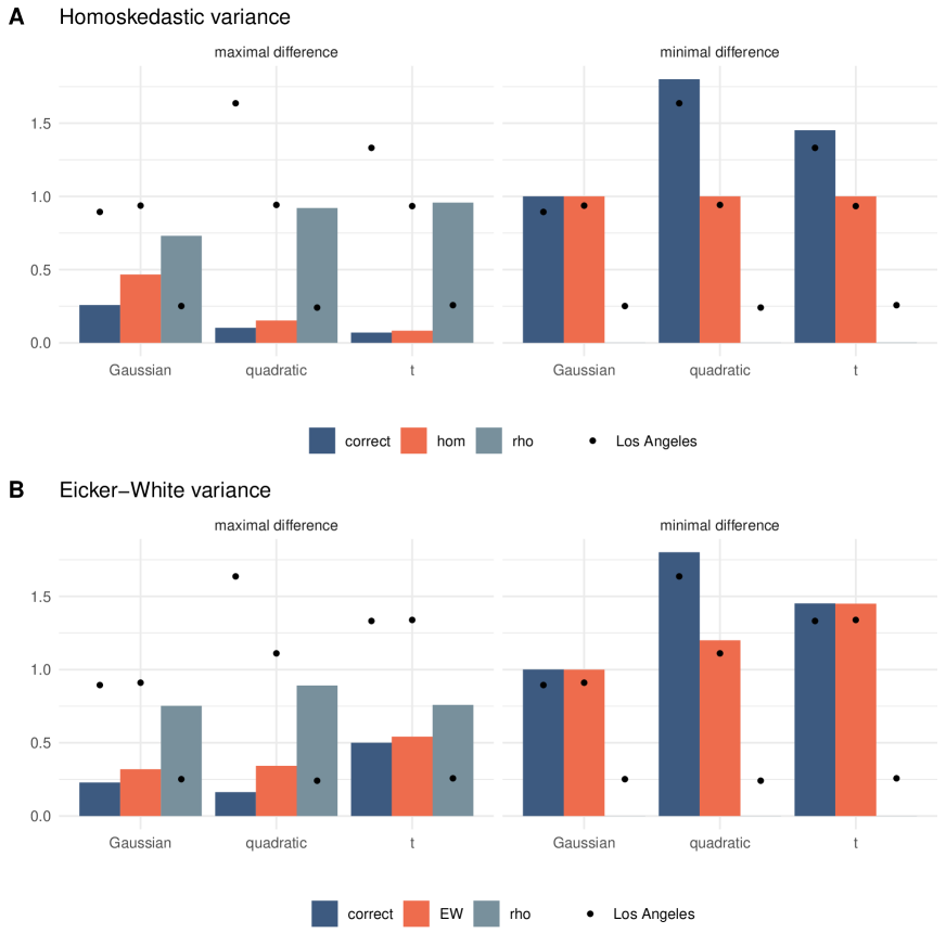
Figure 1: Variances achieving minimal and maximal differences within different families of copulas. Specifications and details can be found in Appendix A. “correct” refers to $\sigma^{2}$, “hom” to $\sigma_{hom}^{2}$, “EW” to $\sigma_{EW}^{2}$, and “rho” to the rank correlation of the copula achieving the optimized difference. The dots indicate the rank correlation in Los Angeles and the implied variances for the particular copula within the parametric family that corresponds to that rank correlation.

Specifically, we compute the minimal and maximal differences $\sigma_{hom}^{2}-\sigma^{2}$ and $\sigma_{EW}^{2}-\sigma^{2}$ over three families of copulas: the Gaussian, the Student-t (“t”), and a “quadratic” copula. In all cases, we optimize over the parameters of the copulas so as to find the largest and smallest difference in variances. Details of the specifications and solutions of the optimization problems can be found in Appendix A.2.

Panels A and B in Figure 1 show the variances achieving the minimal and maximal differences for the homoskedastic (“hom”) and the Eicker-White (“EW”) variances within the different families of copulas. They also display the rank correlation $\rho$ of the copulas that achieve the optima. The optimal copulas achieving these bounds are shown in Figures 14–16 in Appendix A.2. Within the t and the quadratic families, the correct variance $\sigma^{2}$ may be substantially larger than the hom and EW variances, up to about 70% larger. Within the Gaussian family this is not possible, but the correct variance may be significantly smaller than the other two, almost half as large. Within the quadratic and the t families, the correct variance may also be smaller than the other two, but to a lesser extent than in the Gaussian family.

Interestingly, the minimal difference in variances is achieved for copulas that have rank correlation close to zero whereas the maximal differences occur for copulas with high rank correlation. To show that substantial differences in variances occur not only for very small or very large rank correlations, the graphs also indicate the value of the three different variances for the copula that matches the rank correlation of child and parent incomes in Los Angeles, one of the commuting zones that we further analyze in Section 5.1. In the data by Chetty et al. (2022a), Los Angeles has a rank correlation of $0.254$. Since individual-level incomes are not publicly available, we do not know the true copula of incomes in Los Angeles. The dots in Figure 1 indicate the values of the correct, the hom, and the EW variances if the copula were Gaussian, t, or quadratic. If it were Gaussian, the hom and EW variances would be slightly larger than the correct one. If it were quadratic, however, the hom and EW variances would both be substantially smaller than the correct variance. Finally, in the t family, the hom variance would be substantially smaller than the correct variance, but the EW variance would be about the same as the correct one.

The variances $\sigma^{2}$, $\sigma_{hom}^{2}$, and $\sigma_{EW}^{2}$ are all bounded, and so mutual differences between them are bounded as well. This is not true for ratios, however. The following lemma shows that if we do not restrict the distributions $F$, the ratios $\sigma_{hom}^{2}/\sigma^{2}$ and $\sigma_{EW}^{2}/\sigma^{2}$ can both be arbitrarily large. To emphasize the dependence of the variances on the joint distribution $F$ of $(X,Y)$, we use the notation $\sigma_{hom}^{2}(F)$, $\sigma_{EW}^{2}(F)$, and $\sigma^{2}(F)$.

Lemma 2.

There exists a sequence $\{F_{k}\}_{k\geq 1}$ of distributions on $\mathbb{R}^{2}$ with continuous marginals such that $\sigma_{hom}^{2}(F_{k})/\sigma^{2}(F_{k})\to\infty$ and $\sigma_{EW}^{2}(F_{k})/\sigma^{2}(F_{k})\to\infty$ as $k\to\infty$.

An implication of this lemma is that the two variances $\sigma_{hom}^{2}$ and $\sigma_{EW}^{2}$ can be larger than the correct variance by arbitrarily large factors. As the proof of the lemma reveals, the divergence occurs under sequences of copulas approaching perfect dependence so that both variances tend to zero, but the correct variance converges to zero at a faster rate than the variances $\sigma_{hom}^{2}$ and $\sigma_{EW}^{2}$.

Given the result in Lemma 2, the next interesting question is how small the variances $\sigma_{hom}^{2}$ and $\sigma_{EW}^{2}$ can be relative to the true variance $\sigma^{2}$. The following lemma provides a partial answer to this question in the case of $\sigma_{hom}^{2}$.

Lemma 3.

There exists a constant $c>0$ such that $\sigma_{hom}^{2}(F)/\sigma^{2}(F)\geq c$ for all distributions $F$ on $\mathbb{R}^{2}$ with continuous marginals.

By this lemma, the ratio $\sigma_{hom}^{2}/\sigma^{2}$ is bounded away from zero, so that $\sigma_{hom}^{2}$ can be smaller than $\sigma^{2}$ only by a factor that is bounded from below by the constant $c$. However, it is important to emphasize that this constant may be rather small. In particular, we have already seen in Figure 1 that for simple well-known classes of copulas, like the t copula, the hom variance may be substantially smaller than the correct variance. In the empirical applications of Section 5, we also find that the hom variance may be substantially smaller than the correct variance.

In conclusion, this subsection has shown that commonly used formulas for the estimation of asymptotic variances, and thus also for standard errors, do not yield the correct asymptotic variance of the OLS estimator in a rank-rank regression. In particular, the homoskedastic and the Eicker-White standard errors may be too small or too large depending on the shape of the copula of the income distribution. In consequence, confidence intervals may be too short or too wide, possibly leading to under-coverage or conservative inference.

2.2 Rank-Rank Regressions With Noncontinuous Marginal Distributions

The well-established asymptotic theory for Spearman’s rank correlation described in the previous subsection crucially depends on the assumption that both marginals of the distribution $F$ are continuous. In empirical applications of rank-rank regressions, however, pointmasses are common. For instance, incomes may be top-coded, there may be pointmasses at zero or negative incomes (e.g. as in Chetty and Hendren (2018)). In fact, one of the commonly cited (Deutscher and Mazumder (2023), Mogstad and Torsvik (2023)) advantages of studying the rank-rank relationship over other approaches such as estimating intergenerational elasticities is that the rank-based approach is applicable in the presence of zero incomes. In addition, income measurements may be rounded, or ranks may be computed from discrete measures other than income (e.g., occupational status as in Ward (2022a) or human capital as in de la Croix and Goni (2022)). In such cases, pointmasses in the income distribution create ties in the ranks and their presence changes inference in the rank-rank regression in at least three important ways: (i) the interpretation of the estimand in the rank-rank regression changes, (ii) the estimand changes with the way in which ties are handled, and (iii) the statistical properties of the OLS estimator change with the way ties are handled. We now illustrate each of these three points in more detail.

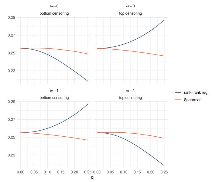
Figure 2: Spearman’s rank correlation (“Spearman”) and the slope coefficient from a rank-rank regression (“rank-rank reg”), where $Y$ is a child’s income and $X$ their parent’s income. The graphs in the first column (“bottom censoring”) show the two estimates when all parental incomes up to the $q$-th quantile are set to zero, while those in the second column (“top censoring”) show the same quantities when all parental incomes above the $(1-q)$-th quantile are set equal to the income at that quantile. $\omega$ denotes the definition of the rank as in (9) below, i.e. $\omega=0$ ($\omega=1$) leads to smallest (largest) possible rank assigned to ties. Incomes are drawn from the (continuous) calibrated income distribution of Los Angeles as in Section 5.1 using the Gaussian copula and log-normal marginals, and then parental incomes are censored. The estimates are computed on a single, but very large sample (of size $10^{6}$), so the estimates are expected to be close to their probability limits.

First, in the presence of pointmasses, the OLS estimator of the rank-rank regression is not equal to Spearman’s rank correlation and its probability limit cannot be interpreted as a rank correlation anymore. This is because the ratio of standard deviations in (2) is not necessarily equal to one. The OLS estimator therefore estimates a scaled version of the rank correlation, which may be scaled upwards or downwards depending on the relative location and magnitudes of pointmasses in the distributions of $X$ and $Y$. In particular, the slope coefficient of the rank-rank regression may lie outside of the $[-1,1]$ interval and cannot be interpreted as a correlation. Researchers should therefore be careful about whether they want to estimate Spearman’s rank correlation or the rank-rank slope, and potentially adjust the rank-rank slope by the ratio of standard deviations.

The first row of Figure 2 illustrates this point. It is based on the (continuous) joint distribution of child and parent incomes which we calibrated to data from Los Angeles (see Section 5.1). We introduce more and more zero (“bottom censoring”) or top-coded (“top censoring”) parental incomes into the distribution and then show how Spearman’s rank correlation (“Spearman”) and the rank-rank slope (“rank-rank reg”) change. The first graph (“bottom censoring”) shows the two estimands when all parental incomes up to the $q$-th quantile are set to zero, while the second graph (“top censoring”) shows the same quantities when all parental incomes above the $(1-q)$-th quantile are set equal to the income at that quantile. At $q=0$ there is no censoring and the joint distribution of incomes is continuous, so the rank correlation and rank-rank slope are equal. With more censoring (larger $q$), the joint distribution features larger pointmasses and the two estimands diverge. Without censoring, the rank-rank slope is equal to $0.254$ while with 25% top-censoring, the rank-rank slope takes a value of $0.287$. Among the ranking of all 709 CZs that we analyze, this change in mobility corresponds to Los Angeles moving from 59th place to 134th place. This is a substantial change in mobility. Of course, 25% of the sample being censored is an extreme case, but we see significant sensitivity of the rank-rank slope with respect to $q$ even for smaller values. In addition, discreteness stemming from sources other than censoring may have similarly substantial impacts on the estimand.

While for top-censoring, the rank-rank slope increases with $q$, for bottom-censoring it decreases with $q$.

Second, in the presence of pointmasses in the distribution $F$, different ways of handling ties in the ranks lead to different estimands (i.e., the rank-rank slopes). The second row in Figure 2 illustrates this point. It shows the same graphs as the first row, but for a different definition of the rank. The rank correlation is almost the same for the two definitions of the rank, but the rank-rank slope substantially changes. Handling ties differently ($\omega=1$) than in the first row of figures ($\omega=0$) means that Los Angeles’ mobility measure drops from $0.254$ without censoring to $0.218$ with 25% top-censoring. This change in mobility corresponds to Los Angeles moving from 59th place up to 20th place in the ranking of all 709 CZs.

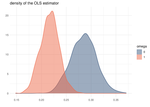
Figure 3: Estimated density of the OLS estimator of the rank-rank slope with two different ways of handling ties (as indicated by the value of $\omega$). The densities are estimated based on simulated data from the income distribution calibrated to data from Los Angeles with 25% top-censoring.

Third, the way in which ties are handled also impacts the statistical properties of the OLS estimator of the rank-rank slope. Figure 3 illustrates this point by showing the estimated distribution of the estimator for the two different definitions of the ranks for $\omega=0$ and $\omega=1$. To create this graph, we simulated 10,000 samples of size 2,000 from the income distribution calibrated to data from Los Angeles with 25% top-coding and the Gaussian copula. In Figure 2, we have already seen how the estimand changes depending on whether $\omega=0$ or $\omega=1$. In Figure 3, we see this reflected in the different means of the two distributions of the estimator. In addition, however, the variance of the two estimators is also different. If ties are handled by setting $\omega=0$, the variance is larger compared to the estimator’s variance when $\omega=1$.

2.3 Summary

The previous arguments can be summarized as follows:

1. Hoeffding (1948)’s derivation of the asymptotic distribution of Spearman’s rank correlation yields the correct asymptotic distribution of the OLS estimator of the slope in a rank-rank regression in the special case with continuous marginal distributions of $Y$ and $X$ and without covariates.

2. Commonly used variance estimators for OLS regressions do not estimate this asymptotic variance. They may be too small or too large depending on the shape of the copula of the pair $(X,Y)$.

3. When at least one of the two marginal distributions of $Y$ and $X$ is not continuous or when there are covariates in the regression, then Hoeffding’s theory does not apply. Importantly, in the noncontinuous case, the rank-rank regression estimand, the OLS estimator, and its asymptotic distribution are all sensitive to the specific way in which ties are handled.

The next section develops a general, unifying asymptotic theory for coefficients in a rank-rank regression that allows for any definition of the rank, for continuous or noncontinuous distributions, and for the presence of covariates.

3 Inference for Rank-Rank Regressions

3.1 Asymptotic Normality Result

In this section, we develop the asymptotic theory for the OLS estimator of a rank-rank regression. The results apply to continuous and non-continuous distributions $F$. To deal with potential ties, we consider a more general definition of the rank, in fact a class of ranks, indexed by a parameter $\omega\in[0,1]$. Different definitions of the rank differ in the way in which they handle ties, but they are all equivalent in the absence of ties.

For a fixed, user-specified $\omega\in[0,1]$, let $F_{X}^{-}(x):=P(X<x)$, $I(u,v):=\omega\mathds{1}\{u\leq v\}+(1-\omega)\mathds{1}\{u<v\}$, and

$$R_{X}(x):=\omega F_{X}(x)+(1-\omega)F_{X}^{-}(x),\quad x\in\mathbb{R}.$$

For an i.i.d. sample $X_{1},\ldots,X_{n}$ from $F_{X}$, we then define the rank of $i$ as $R_{i}^{X}:=\widehat{R}_{X}(X_{i})$, where

$$\widehat{R}_{X}(x):=\omega\widehat{F}_{X}(x)+(1-\omega)\widehat{F}_{X}^{-}(x)+\frac{1-\omega}{n},\quad x\in\mathbb{R},$$ (9)

is an estimator of $R_{X}(x)$. This definition of the rank is such that an individual $i$ with a large value of $X_{i}$ is assigned a large rank. If $F_{X}$ is continuous, then the probability of a tie among $X_{1},\ldots,X_{n}$ is zero and the rank $R_{i}^{X}$ is the same for all values of $\omega$. If $F_{X}$ is not continuous, then different choices of $\omega$ lead to definitions of the rank that handle ties differently. For instance, if $\omega=1$ then $R_{i}^{X}=\widehat{F}_{X}(X_{i})$ and tied individuals are assigned the largest possible rank. If $\omega=1/2$, then $R_{i}^{X}$ is the mid-rank as defined in Hoeffding (1948), which assigns to tied individuals the average of the smallest and largest possible ranks. Finally, $\omega=0$ leads to a definition of the rank that assigns to tied individuals the smallest possible rank. Table 1 illustrates the different definitions of ranks in an example with ties. The quantities $F_{Y}$, $F_{Y}^{-}$, $R_{Y}$ and their estimators are defined analogously for $Y$. We assume that $\omega$ is the same value in $R_{X}$ and $R_{Y}$, so that ranks are defined consistently for both variables $X$ and $Y$. Throughout the paper, this value of $\omega$ is fixed and chosen by the researcher, so it does not appear as argument or index anywhere.

$i$	1	2	3	4	5	6	7	8	9	10
$X_{i}$	3	4	7	7	10	11	15	15	15	15
smallest rank: $R_{i}^{X}$ for $\omega=0$	0.1	0.2	0.3	0.3	0.5	0.6	0.7	0.7	0.7	0.7
mid-rank: $R_{i}^{X}$ for $\omega=0.5$	0.1	0.2	0.35	0.35	0.5	0.6	0.85	0.85	0.85	0.85
largest rank: $R_{i}^{X}$ for $\omega=1$	0.1	0.2	0.4	0.4	0.5	0.6	1	1	1	1

Table 1: example of three different definitions of ranks for a given sample. Bold columns indicate ties.

We consider the following regression model:

$$R_{Y}(Y)=\rho R_{X}(X)+W^{\prime}\beta+\varepsilon,\qquad E\left[\varepsilon\begin{pmatrix}R_{X}(X)\\ W\end{pmatrix}\right]=0,$$ (10)

where $W$ is a $d$-dimensional vector of covariates, $\varepsilon$ is noise, and $\rho$, $\beta$ are regression coefficients to be estimated. As already indicated in Section 2.2, the interpretation of $\rho$ depends on whether the marginal distributions of $Y$ and $X$ are continuous and, if at least one of them is not, how ties are handled. However, in the model (10) there is one additional reason complicating the interpretation of $\rho$, namely the presence of covariates: even if $Y$ and $X$ have continuous marginal distributions, in the presence of covariates $W$ that are correlated with $X$, $\rho$ cannot be interpreted as a rank correlation and, in particular, does not have to lie in the interval $[-1,1]$.

Letting $\{(X_{i},W_{i},Y_{i})\}_{i=1}^{n}$ be an i.i.d. sample from the distribution of the triplet $(X,W,Y)$, we study the properties of the following OLS estimator of the vector of parameters $(\rho,\beta^{\prime})^{\prime}$:

$$\begin{pmatrix}\widehat{\rho}\\ \widehat{\beta}\end{pmatrix}=\left(\sum_{i=1}^{n}\begin{pmatrix}R_{i}^{X}\\ W_{i}\end{pmatrix}\begin{pmatrix}R_{i}^{X}&W_{i}^{\prime}\end{pmatrix}\right)^{-1}\sum_{i=1}^{n}\begin{pmatrix}R_{i}^{X}\\ W_{i}\end{pmatrix}R_{i}^{Y}.$$ (11)

To derive the asymptotic normality of $\widehat{\rho}$, we introduce the projection of $R_{X}(X)$ onto the covariates:

$$R_{X}(X)=W^{\prime}\gamma+\nu,\quad E[\nu W]=0,$$ (12)

where $\nu$ is a random variable representing the projection residual, and $\gamma$ is a vector of parameters. Consider the following regularity conditions:

Assumption 1.

$\{(X_{i},W_{i},Y_{i})\}_{i=1}^{n}$ is an i.i.d. sample from the distribution of $(X,W,Y)$.

Assumption 2.

The vector $W$ satisfies $E[\|W\|^{4}]<\infty$ and the matrix $E[WW^{\prime}]$ is non-singular.

Assumption 3.

The random variable $\nu$ is such that $E[\nu^{2}]>0$.

These are standard regularity conditions underlying typical regression analysis. Assumption 3 requires that the rank $R_{X}(X)$ can not be represented as a linear combination of covariates. Importantly, our regularity conditions do not require $X$ and $Y$ to be continuously distributed.

Under these conditions, we have the following asymptotic normality result.

Theorem 1.

Suppose that (10)–(12) hold and that Assumptions 1–3 are satisfied. Then

$$\sqrt{n}(\widehat{\rho}-\rho)=\frac{1}{\sigma_{\nu}^{2}\sqrt{n}}\sum_{i=1}^{n}\Big{\{}h_{1}(X_{i},W_{i},Y_{i})+h_{2}(X_{i},Y_{i})+h_{3}(X_{i})\Big{\}}+o_{P}(1)\to_{D}N(0,\sigma^{2}),$$

where

$$\sigma^{2}:=\frac{1}{\sigma_{\nu}^{4}}E\Big{[}(h_{1}(X,W,Y)+h_{2}(X,Y)+h_{3}(X))^{2}\Big{]}$$ (13)

with $\sigma_{\nu}^{2}:=E[\nu^{2}]$ and

$$h_{1}(x,w,y) :=(R_{Y}(y)-\rho R_{X}(x)-w^{\prime}\beta)(R_{X}(x)-w^{\prime}\gamma),$$

$$h_{2}(x,y) :=E[(I(y,Y)-\rho I(x,X)-W^{\prime}\beta)(R_{X}(X)-W^{\prime}\gamma)],$$

$$h_{3}(x) :=E[(R_{Y}(Y)-\rho R_{X}(X)-W^{\prime}\beta)(I(x,X)-W^{\prime}\gamma)]$$

for all $x\in\mathbb{R}$, $w\in\mathbb{R}^{p}$, and $y\in\mathbb{R}$.

As already mentioned above, the proof of this result, as well as of all other results presented in this paper, can be found in Appendix C. In fact, Theorem 1 follows from a more general result, which we state in Appendix B (Theorem 5). The more general result shows joint asymptotic normality for $\widehat{\rho}$ and $\widehat{\beta}$,

$$\sqrt{n}\begin{pmatrix}\widehat{\rho}-\rho\\ \widehat{\beta}-\beta\end{pmatrix}=\frac{1}{\sqrt{n}}\sum_{i=1}^{n}\psi_{i}+o_{P}(1)\to_{D}N(0,\Sigma),\qquad\Sigma:=E[\psi_{i}\psi_{i}^{\prime}],$$

and provides an explicit formula for $\psi_{i}$. The joint asymptotic distribution for $\widehat{\rho}$ and $\widehat{\beta}$ is useful for empirical work in the intergenerational mobility literature. Suppose there are no covariates so $W$ only contains a constant. Besides the rank-rank slope, another popular measure of intergenerational mobility (Deutscher and Mazumder (2023)) is the expected income rank of a child given that their parent’s income rank is equal to some given value $p$:

$$\theta_{p}:=\beta+\rho\,p.$$

With the asymptotic joint distribution above, it is straightforward to compute standard errors and confidence intervals for $\theta_{p}$.

Theorem 1 has the following interpretation. If we knew the population ranks $R_{Y}(Y_{i})$ and $R_{X}(X_{i})$, we would simply estimate $\rho$ and $\beta$ by an OLS regression of $R_{Y}(Y_{i})$ on $R_{X}(X_{i})$ and $W$. The asymptotic variance of such an estimator for $\rho$ would be given by $E[h_{1}(X,W,Y)^{2}]/\sigma_{\nu}^{2}$, which is the familiar OLS variance formula. Without knowing the population ranks, however, we have to plugin their estimators, and the extra terms in the asymptotic variance, represented by $h_{2}(X,Y)$ and $h_{3}(X)$, provide the adjustments necessary to take into account the noise coming from estimated ranks. Importantly, the estimation error in the ranks is of the same order of magnitude as that in the OLS estimator with known ranks. Therefore, the estimation error in the ranks does not become negligible in large samples, not even in the limit as the sample size grows to infinity.

The derivation of the asymptotic normality result uses standard techniques from the U-statistic theory. To see this consider the case without covariates so that $W$ only contains a constant. Then, the OLS estimator of the slope can be written as

$$\widehat{\rho}=\frac{\frac{1}{n}\sum_{i=1}^{n}(R_{i}^{Y}-\bar{R}^{Y})(R_{i}^{X}-\bar{R}^{X})}{\frac{1}{n}\sum_{i=1}^{n}(R_{i}^{X}-\bar{R}^{X})^{2}}.$$

It is easy to show that the denominator converges in probability to $\sigma_{\nu}^{2}$. The numerator is a U-statistic because it is an average of terms involving $R_{i}^{Y}$ and $R_{i}^{X}$, which themselves are sample averages. Under the above assumptions one can then verify the standard conditions for such a U-statistic to be asymptotically normal (e.g., Serfling (2002)).

Remark (Comparing the variance formulas in (4) and (13)).

When both $X$ and $Y$ are continuous random variables and $W$ contains only a constant, the asymptotic variance formula in (13) reduces to the classical Hoeffding variance formula in (4). Indeed, replacing $X$ and $Y$ by $F_{X}(X)$ and $F_{Y}(Y)$ respectively, we can assume without loss of generality that both $X$ and $Y$ are $U([0,1])$ random variables, in which case $\psi_{X}(x)$ in (5) reduces to

$$\int_{0}^{1}(E[\mathds{1}\{X\leq x\}\mathds{1}\{Y\leq y\}]-xy)dy=E[\mathds{1}\{X\leq x\}(1-Y)]-x/2=x/2-E[\mathds{1}\{X\leq x\}Y].$$

Similarly, $\psi_{Y}(y)$ in (6) reduces to $y/2-E[\mathds{1}\{Y\leq y\}X]$. Hence, the variance in (4) simplifies to $\sigma^{2}=144Var(h(X,Y))$, where

$$h(x,y):=xy-E[\mathds{1}\{X\leq x\}Y]-E[\mathds{1}\{Y\leq y\}X],\quad x\in\mathbb{R},y\in\mathbb{R},$$ (14)

and it is straightforward to verify that $h(x,y)$ coincides with $h_{1}(x,w,y)+h_{2}(x,y)+h_{3}(x)$ up to an additive constant whenever $X,Y\sim U([0,1])$ and $W$ contains only a constant. $\square$

Remark (Asymptotic variance in the non-continuous case).

The asymptotic normality result in Theorem 1 holds for both continuous and noncontinuous distributions of $Y$ and $X$. In the presence of pointmasses in at least one of the distributions of $Y$ and $X$, although implicitly, the asymptotic variance $\sigma^{2}$ of the OLS estimator derived in Theorem 1 depends on $\omega$. Therefore, different ways of handling ties through different choices of $\omega$ may affect not only the estimand and the estimator, but also the value of the asymptotic variance, as we have already seen in the discussion of Figure 3. $\square$

3.2 Consistent Estimation of the Asymptotic Variance

In this subsection, we propose an estimator of the asymptotic variance $\sigma^{2}$ appearing in the asymptotic normality result in Theorem 1 and show that it is consistent. In particular, we consider the following plug-in estimator:

$$\widehat{\sigma}^{2}:=\frac{1}{n\widehat{\sigma}_{\nu}^{4}}\sum_{i=1}^{n}(H_{1i}+H_{2i}+H_{3i})^{2},$$

where $\widehat{\sigma}_{\nu}^{2}:=n^{-1}\sum_{i=1}^{n}\widehat{\nu}_{i}^{2}$ is an empirical analog of $\sigma_{\nu}^{2}=E[\nu^{2}]$, $\widehat{\nu}_{i}:=R_{i}^{X}-W_{i}^{\prime}\widehat{\gamma}$, and

$$H_{1i} :=\left(R_{i}^{Y}-\widehat{\rho}R_{i}^{X}-W_{i}^{\prime}\widehat{\beta}\right)\left(R_{i}^{X}-W_{i}^{\prime}\widehat{\gamma}\right),$$

$$H_{2i} :=\frac{1}{n}\sum_{j=1}^{n}\left(I(Y_{i},Y_{j})-\widehat{\rho}I(X_{i},X_{j})-W_{j}^{\prime}\widehat{\beta}\right)\left(R_{j}^{X}-W_{j}^{\prime}\widehat{\gamma}\right),$$

$$H_{3i} :=\frac{1}{n}\sum_{j=1}^{n}\left(R_{j}^{Y}-\widehat{\rho}R_{j}^{X}-W_{j}^{\prime}\widehat{\beta}\right)\left(I(X_{i},X_{j})-W_{j}^{\prime}\widehat{\gamma}\right),$$

for all $i=1,\dots,n$. The following lemma shows that this simple plug-in estimator is consistent without any additional assumptions.

Lemma 4.

Suppose that (10)–(12) hold and that Assumptions 1–3 are satisfied. Then $\widehat{\sigma}^{2}\to_{P}\sigma^{2}$.

Theorem 1 and Lemma 4 give the correct way to perform inference in rank-rank regressions. For example, a $(1-\alpha)\times 100\%$ asymptotic confidence interval for $\rho$ can be constructed using the standard formula

$$\left(\widehat{\rho}-\frac{z_{\alpha/2}\widehat{\sigma}}{\sqrt{n}},\widehat{\rho}+\frac{z_{\alpha/2}\widehat{\sigma}}{\sqrt{n}}\right),$$

where $z_{\alpha/2}$ is the number such that $P(N(0,1)>z_{\alpha/2})=\alpha/2$. Standard hypothesis testing can be performed analogously.

Remark (Bootstrapping the distribution of $\sqrt{n}(\widehat{\rho}-\rho)$).

In addition, to performing inference on $\rho$ via a consistent estimator of the asymptotic variance $\widehat{\sigma}^{2}$ in Lemma 4, one can also perform inference by bootstrapping the distribution of $\sqrt{n}(\widehat{\rho}-\rho)$. Indeed, to show bootstrap validity, observe that $\rho=\rho(F)$ is a smooth functional (Hadamard differentiable), and our estimator $\widehat{\rho}$ takes the plug-in form, $\widehat{\rho}=\rho(\widehat{F})$. Therefore, given that the empirical distribution function $\widehat{F}$ satisfies Donsker’s theorem, it follows from Theorem 3.1 in Fang and Santos (2019) that the distribution of $\sqrt{n}(\widehat{\rho}^{*}-\widehat{\rho})$, where $\widehat{\rho}^{*}$ is the estimator $\widehat{\rho}$ obtained on a bootstrap sample, consistently estimates that of $\sqrt{n}(\widehat{\rho}-\rho)$; see also Bickel and Freedman (1981) for the original result on bootstrapping von Mises functionals. $\square$

4 Inference for Other Regressions Involving Ranks

Motivated by regressions that have been used in empirical work, especially in the intergenerational mobility literature, we provide three extensions of the asymptotic normality result in Theorem 1. In particular, we consider (i) a rank-rank regression with clusters, where ranks are computed in the national distributions rather than in the cluster-specific distributions, (ii) a regression of a general outcome $Y$ on the rank $R_{X}(X)$, and (iii) a regression of the rank $R_{Y}(Y)$ on a covariate $X$. For brevity of the paper, we keep the discussions of each extension relatively short.

4.1 Rank-Rank Regressions With Clusters

In this subsection, we consider a population (e.g., the U.S.) that is divided into $n_{G}$ subpopulations or “clusters” (e.g., commuting zones). We are interested in running rank-rank regressions separately within each cluster. The ranks, however, are computed from the distribution of the entire population (e.g., the U.S.). Such regressions have become particularly popular since the influential work by Chetty et al. (2014) for studying regional mobility, where the scale of the mobility measure is fixed by the national distribution. The survey by Deutscher and Mazumder (2023) provides more examples of empirical work running such regressions, for instance Corak (2020) and Acciari et al. (2022).

Specifically, we consider the model

$$R_{Y}(Y)=\sum_{g=1}^{n_{G}}\mathds{1}\{G=g\}\left(\rho_{g}R_{X}(X)+W^{\prime}\beta_{g}\right)+\varepsilon,\qquad E\left[\left.\varepsilon\begin{pmatrix}R_{X}(X)\\ W\end{pmatrix}\right|G\right]=0\;\text{a.s.},$$ (15)

where $G$ is an observed random variable taking values in $\{1,\ldots,n_{G}\}$ to indicate the cluster to which an individual belongs. The quadruple $(G,X,W,Y)$ has distribution $F$, and we continue to denote marginal distributions of $X$ and $Y$ by $F_{X}$ and $F_{Y}$. The quantities $F_{X}^{-}$, $F_{Y}^{-}$, $R_{X}(x)$, and $R_{Y}(y)$ are also as previously defined, so that $R_{X}(X)$, for instance, is the rank of $X$ in the entire population, not the rank within a cluster. So, in the model (15), the coefficients $\rho_{g}$ and $\beta_{g}$ are cluster-specific, but the ranks $R_{Y}(Y)$ and $R_{X}(X)$ are not. In consequence, $\rho_{g}$ cannot be interpreted as the rank correlation within the cluster $g$. Instead, in the intergenerational mobility literature, the rank-rank slope is interpreted as a relative measure of mobility in a region $g$, where its scale is fixed by the national population. Unlike the rank-rank slope in the model without clusters, (10), the slopes $\rho_{g}$ do not only depend on the copula of $Y$ and $X$ in a cluster, but also on the marginal distributions of $Y$ and $X$ in the cluster. To see this note that adding a fixed amount to every child and parent income in a cluster does not change the ranking of children and parents within the cluster, but it may change the ranking of these individuals in their national income distributions. In conclusion, the $\rho_{g}$ may then also change.

We now introduce a first-stage projection equation similar to the one in (12), except that the coefficients are cluster-specific:

$$R_{X}(X)=\sum_{g=1}^{n_{G}}\mathds{1}\{G=g\}W^{\prime}\gamma_{g}+\nu,\quad E[\left.\nu W\right|G]=0\;\text{a.s.}.$$ (16)

Let $\{(G_{i},X_{i},W_{i},Y_{i})\}_{i=1}^{n}$ be an i.i.d. sample from the distribution of $(G,X,W,Y)$. Ranks are computed using all observations, i.e. $R_{i}^{X}:=\widehat{R}_{X}(X_{i})$ with $\widehat{R}_{X}(x)$ as in (9) and $\widehat{F}_{X}$ ($\widehat{F}^{-}_{X}$) the (left-limit of the) empirical cdf of $X_{1},\ldots,X_{n}$. The computation of the rank $R_{i}^{Y}$ is analogous.

First, notice that an OLS regression of $R_{i}^{Y}$ on all regressors, i.e. $(\mathds{1}\{G_{i}=g\}R_{i}^{X})_{g=1}^{n_{G}}$ and $(\mathds{1}\{G_{i}=g\}W_{i}^{X})_{g=1}^{n_{G}}$, produces estimates $(\widehat{\rho}_{g},\widehat{\beta}_{g})_{g=1}^{n_{G}}$ of $(\rho_{g},\beta_{g})_{g=1}^{n_{G}}$ that can be written as:

$$\begin{pmatrix}\widehat{\rho}_{g}\\ \widehat{\beta}_{g}\end{pmatrix}=\left(\sum_{i=1}^{n}\mathds{1}\{G_{i}=g\}\begin{pmatrix}R_{i}^{X}\\ W_{i}\end{pmatrix}\begin{pmatrix}R_{i}^{X}&W_{i}^{\prime}\end{pmatrix}\right)^{-1}\sum_{i=1}^{n}\mathds{1}\{G_{i}=g\}\begin{pmatrix}R_{i}^{X}\\ W_{i}\end{pmatrix}R_{i}^{Y}.$$ (17)

Therefore, $(\widehat{\rho}_{g},\widehat{\beta}_{g})$ can be computed by an OLS regression of $R_{i}^{Y}$ on $R_{i}^{X}$ and $W_{i}$ using only observations $i$ from cluster $g$. Similarly, $\widehat{\gamma}_{g}$ can be computed by an OLS regression of $R_{i}^{X}$ on $W_{i}$ using only observations $i$ from cluster $g$. Note however, as explained above, that the ranks $R_{i}^{X}$ and $R_{i}^{Y}$ are computed using observations of $X$ and $Y$ from all clusters and thus the OLS estimators across clusters are not independent.

The following are Assumptions 1–3 adapted to the model with clusters:

Assumption 4.

$\{(G_{i},X_{i},W_{i},Y_{i})\}_{i=1}^{n}$ is a random sample from the distribution of $(G,X,W,Y)$.

Assumption 5.

The vector $W$ is such that $E[\|W\|^{4}]<\infty$ and, for all $g=1,\ldots,n_{G}$, the matrix $E[\mathds{1}\{G=g\}WW^{\prime}]$ is non-singular.

Assumption 6.

The random variable $\nu$ is such that $E[\mathds{1}\{G=g\}\nu^{2}]>0$ for all $g=1,\dots,n_{G}$.

As in the previous section, note that our assumptions do not require the marginal distributions $F_{X}$ and $F_{Y}$ to be continuous. In addition, we introduce an assumption about the number and size of the clusters:

Assumption 7.

The number of clusters $n_{G}$ is a finite constant and $P(G=g)>0$ for all $g=1,\ldots,G$.

Observe that if the number of clusters were to increase together with the sample size $n$, with the number of units within each cluster being of the same order, the extra noise coming from estimated ranks would be asymptotically negligible, and the standard OLS variance formula would be applicable. The new result below applies to the case with a fixed number of clusters so that the estimation error in the ranks is not negligible even in large samples. This scenario seems reasonable, for instance, in our empirical application in which a cluster is a commuting zone within a U.S. state because each of these states contains only a small number of commuting zones relative to the sample size.

Under these four assumptions, we have the following extension of Theorem 1.

Theorem 2.

Suppose that (15)–(17) hold and that Assumptions 4–7 are satisfied. Then for all $g=1,\dots,G$, we have

$$\sqrt{n}(\widehat{\rho}_{g}-\rho_{g})=\frac{1}{\sigma_{\nu,g}^{2}\sqrt{n}}\sum_{i=1}^{n}\Big{\{}h_{1,g}(G_{i},X_{i},W_{i},Y_{i})+h_{2,g}(X_{i},Y_{i})+h_{3,g}(X_{i})\Big{\}}+o_{P}(1)\to_{D}N(0,\sigma_{g}^{2}),$$

where

$$\sigma_{g}^{2}:=\frac{1}{\sigma_{\nu,g}^{4}}E\Big{[}(h_{1,g}(G,X,W,Y)+h_{2,g}(X,Y)+h_{3,g}(X))^{2}\Big{]}$$

with $\sigma_{\nu,g}^{2}:=E[\mathds{1}\{G=g\}\nu^{2}]$ and

$$h_{1,g}(\bar{g},x,w,y) :=\mathds{1}\{\bar{g}=g\}(R_{Y}(y)-\rho_{g}R_{X}(x)-w^{\prime}\beta_{g})(R_{X}(x)-w^{\prime}\gamma_{g}),$$

$$h_{2,g}(x,y) :=E[\mathds{1}\{G=g\}(I(y,Y)-\rho_{g}I(x,X)-W^{\prime}\beta_{g})(R_{X}(X)-W^{\prime}\gamma_{g})],$$

$$h_{3,g}(x) :=E[\mathds{1}\{G=g\}(R_{Y}(Y)-\rho_{g}R_{X}(X)-W^{\prime}\beta_{g})(I(x,X)-W^{\prime}\gamma_{g})]$$

for all $\bar{g}\in\{1,\dots,n_{G}\}$, $x\in\mathbb{R}$, $w\in\mathbb{R}^{p}$, and $y\in\mathbb{R}$.

In Appendix B, we provide a joint asymptotic normality result for all regression coefficients. Letting $\widehat{\rho}:=(\widehat{\rho}_{1},\ldots,\widehat{\rho}_{n_{G}})^{\prime}$, $\rho:=(\rho_{1},\ldots,\rho_{n_{G}})^{\prime}$, $\widehat{\beta}:=(\widehat{\beta}_{1}^{\prime},\ldots,\widehat{\beta}_{n_{G}}^{\prime})^{\prime}$, and $\beta:=(\beta_{1}^{\prime},\ldots,\beta_{n_{G}}^{\prime})^{\prime}$, the appendix shows that

$$\sqrt{n}\begin{pmatrix}\widehat{\rho}-\rho\\ \widehat{\beta}-\beta\end{pmatrix}=\frac{1}{\sqrt{n}}\sum_{i=1}^{n}\psi_{i}+o_{P}(1)\to_{D}N(0,\Sigma),\qquad\Sigma:=E[\psi_{i}\psi_{i}^{\prime}],$$ (18)

and provides an explicit formula for $\psi_{i}$. From this result, one can then easily calculate the asymptotic distribution of linear combinations of parameters. For instance, similarly as in the rank-rank regression without clusters, a popular measure of intergenerational mobility (Deutscher and Mazumder (2023)) is the expected rank of a child with parents at a given income rank $p$,

$$\theta_{g,p}:=\beta_{g}+\rho_{g}\;p.$$ (19)

The asymptotic distribution in (18) allows us to construct a confidence interval for $\theta_{g,p}$ for a specific commuting zone $g$ or simultaneous confidence sets across all commuting zones.

An estimator of the asymptotic variance $\sigma^{2}$ is

$$\widehat{\sigma}_{g}^{2}:=\frac{1}{n\widehat{\sigma}_{\nu,g}^{4}}\sum_{i=1}^{n}(H_{1,g,i}+H_{2,g,i}+H_{3,g,i})^{2},$$

where

$$\widehat{\sigma}_{\nu,g}^{2} :=\frac{1}{n}\sum_{i=1}^{n}\mathds{1}\{G_{i}=g\}(R_{i}^{X}-W_{i}^{\prime}\widehat{\gamma}_{g})^{2},$$

$$H_{1,g,i} :=\mathds{1}\{G_{i}=g\}\left(R_{i}^{Y}-\widehat{\rho}_{g}R_{i}^{X}-W_{i}^{\prime}\widehat{\beta}_{g}\right)\left(R_{i}^{X}-W_{i}^{\prime}\widehat{\gamma}_{g}\right),$$

$$H_{2,g,i} :=\frac{1}{n}\sum_{j=1}^{n}\mathds{1}\{G_{j}=g\}\left(I(Y_{i},Y_{j})-\widehat{\rho}_{g}I(X_{i},X_{j})-W_{j}^{\prime}\widehat{\beta}_{g}\right)\left(R_{j}^{X}-W_{j}^{\prime}\widehat{\gamma}_{g}\right),$$

$$H_{3,g,i} :=\frac{1}{n}\sum_{j=1}^{n}\mathds{1}\{G_{j}=g\}\left(R_{j}^{Y}-\widehat{\rho}_{g}R_{j}^{X}-W_{j}^{\prime}\widehat{\beta}_{g}\right)\left(I(X_{i},X_{j})-W_{j}^{\prime}\widehat{\gamma}_{g}\right)$$

for all $g\in\{1,\dots,n_{G}\}$ and $i=1,\dots,n$. One can prove consistency of this estimator using the same arguments as those in the proof of Lemma 4.

4.2 Regression of a General Outcome on a Rank

In this subsection, we consider a regression model with a general outcome $Y$ as the dependent variable and a rank as the regressor:

$$Y=\rho R_{X}(X)+W^{\prime}\beta+\varepsilon,\qquad E\left[\varepsilon\begin{pmatrix}R_{X}(X)\\ W\end{pmatrix}\right]=0.$$ (20)

Such a regression has been used, for instance, by Chetty et al. (2014) to study the association of child outcomes like college attendance or teenage pregnancy with the parent’s income rank. Another example is Chetty et al. (2011) in which wages are regressed on the rank of a test score.

For the above regression, the OLS estimator takes the form

$$\begin{pmatrix}\widehat{\rho}\\ \widehat{\beta}\end{pmatrix}=\left(\sum_{i=1}^{n}\begin{pmatrix}R_{i}^{X}\\ W_{i}\end{pmatrix}\begin{pmatrix}R_{i}^{X}&W_{i}^{\prime}\end{pmatrix}\right)^{-1}\sum_{i=1}^{n}\begin{pmatrix}R_{i}^{X}\\ W_{i}\end{pmatrix}Y_{i}.$$ (21)

The following theorem derives asymptotic normality for $\widehat{\rho}$.

Theorem 3.

Suppose that (12), (20), and (21) hold, that $E[\varepsilon^{4}]<\infty$, and that Assumptions 1–3 are satisfied. Then

$$\sqrt{n}(\widehat{\rho}-\rho)=\frac{1}{\sigma_{\nu}^{2}\sqrt{n}}\sum_{i=1}^{n}\Big{\{}h_{1}(X_{i},W_{i},Y_{i})+h_{2}(X_{i})+h_{3}(X_{i})\Big{\}}+o_{P}(1)\to_{D}N(0,\sigma^{2}),$$

where

$$\sigma^{2}:=\frac{1}{\sigma_{\nu}^{4}}E\Big{[}(h_{1}(X,W,Y)+h_{2}(X)+h_{3}(X))^{2}\Big{]}$$

with $\sigma_{\nu}^{2}:=E[\nu^{2}]$ and

$$h_{1}(x,w,y) :=(y-\rho R_{X}(x)-w^{\prime}\beta)(R_{X}(x)-w^{\prime}\gamma),$$

$$h_{2}(x) :=E[Y-\rho I(x,X)-W^{\prime}\beta)(R_{X}(X)-W^{\prime}\gamma)],$$

$$h_{3}(x) :=E[(Y-\rho R_{X}(X)-W^{\prime}\beta)(I(x,X)-W^{\prime}\gamma)]$$

for all $x\in\mathbb{R}$, $w\in\mathbb{R}^{p}$, and $y\in\mathbb{R}$.

In Appendix B, we provide a joint asymptotic normality result for all regression coefficients, i.e. we show that

$$\sqrt{n}\begin{pmatrix}\widehat{\rho}-\rho\\ \widehat{\beta}-\beta\end{pmatrix}=\frac{1}{\sqrt{n}}\sum_{i=1}^{n}\psi_{i}+o_{P}(1)\to_{D}N(0,\Sigma),\qquad\Sigma:=E[\psi_{i}\psi_{i}^{\prime}],$$

and derive the expression for $\psi_{i}$. A consistent estimator of the asymptotic variance can be obtained by the plugin method, analogously to our discussion in Section 3.

4.3 Regression of a Rank on a General Regressor

In this subsection, we consider a regression model with the rank as a dependent variable and a general regressor:

$$R_{Y}(Y)=W^{\prime}\beta+\varepsilon,\qquad E\left[\varepsilon W\right]=0,$$ (22)

where, for brevity of notations, we let the vector $W$ to absorb the regressor $X$. An example of such a regression in applied work is Sharkey and Torrats-Espinosa (2017) who regress the income rank on the crime rate.

Denote by $W_{l}$ the $l$-th element of $W:=(W_{1},\ldots,W_{p})^{\prime}$ and by $W_{-l}$ the vector of all elements of $W$ except the $l$-th. The projection of $W_{l}$ onto $W_{-l}$ for any $l=1,\ldots,p$ now takes the following form:

$$W_{l}=W_{-l}^{\prime}\gamma_{l}+\nu_{l},\quad E[\nu_{l}W_{-l}]=0,$$ (23)

where $\gamma_{1},\ldots,\gamma_{p}$ are $(p-1)$-dimensional vectors of parameters. For this model, the OLS estimator takes the following form:

$$\widehat{\beta}=\left(\sum_{i=1}^{n}W_{i}W_{i}^{\prime}\right)^{-1}\sum_{i=1}^{n}W_{i}R^{Y}_{i}.$$ (24)

We then have the following result.

Theorem 4.

Suppose that (22)–(24) hold and that Assumptions 1 and 2 are satisfied. Then

$$\sqrt{n}(\widehat{\beta}-\beta)=\frac{1}{\sqrt{n}}\sum_{i=1}^{n}\psi_{i}+o_{P}(1)\to_{D}N(0,\Sigma),$$

where $\Sigma:=E[\psi_{i}\psi_{i}^{\prime}]$, $\psi_{i}:=(\phi_{1}(W_{i},Y_{i}),\ldots,\phi_{p}(W_{i},Y_{i})^{\prime}$ for all $i=1,\dots,n$,

$$\phi_{l}(w,y):=\frac{1}{\sigma_{\nu_{l}}^{2}}\left[h_{l,1}(w,y)+h_{l,2}(y)\right],$$

$\sigma_{\nu_{l}}^{2}:=E[\nu_{l}^{2}]$, and

$$h_{l,1}(w,y) :=(R_{Y}(y)-w^{\prime}\beta)(w_{l}-w_{-l}^{\prime}\gamma_{l}),$$

$$h_{l,2}(y) :=E[(I(y,Y)-W^{\prime}\beta)(W_{l}-W_{-l}^{\prime}\gamma_{l})],$$

for all $w\in\mathbb{R}^{p}$ and $y\in\mathbb{R}$.

The theorem shows, in particular, that for the $l$-th element of $\widehat{\beta}$, we have

$$\sqrt{n}(\widehat{\beta}_{l}-\beta_{l})\to_{D}N(0,\sigma_{\beta_{l}}^{2}),$$

where

$$\sigma_{\beta_{l}}^{2}:=\frac{1}{\sigma_{\nu_{l}}^{4}}E\left[\left(h_{l,1}(W,Y)+h_{l,2}(Y)\right)^{2}\right],$$

and, like above, a consistent estimator of the asymptotic variance can be obtained by the plugin method, analogously to our discussion in Section 3.

5 Empirical Applications

We illustrate our new inference methods through three empirical applications: (i) estimating intergenerational income mobility for neighborhoods in the U.S., (ii) estimating intergenerational mobility in terms of occupational status, and (iii) studying the determinants of replicability of laboratory experiments.

5.1 Intergenerational Mobility in the U.S. – Income

In this section, we apply our new inference methods to the analysis of intergenerational mobility in U.S. commuting zones (CZs) as in Chetty et al. (2014, 2018); Chetty and Hendren (2018). Since the micro-data are not publicly available, we design a simulation experiment calibrated to the available information about commuting zones’ income distributions.

Suppose we are interested in learning about mobility in CZs of California. A local politician in a given CZ of the state may be interested in estimating mobility in their own CZ. In that case, she might run a rank-rank regression as in (10) using only data from that particular CZ. Importantly, ranks for children and parents are therefore computed in their respective distributions within that CZ. Second, a state-level politician may want to learn about mobility in all CZs of their state and perhaps compare mobility across CZs. In that case, she might want to run a rank-rank regression with clusters as in (15), where ranks are computed in the distribution of the whole state.

We apply our new inference methods to both types of regressions on simulated data, where the data-generating process has been calibrated to information from the CZs in California, and compare the results to methods using the homoskedastic and Eicker-White variance estimators. Subsequently, we show that the results from California are not special in the sense that similar results are found in other U.S. states.

In both types of regressions, the CZ-specific regressions of the form (10) and the regression with clusters as in (15), $W$ contains only a constant. Both regressions produce rank-rank slopes $\rho_{g}$ for each CZ $g$. In addition, we compute the expected income rank of a child with parents at the $p$-th rank, $\theta_{g,p}$ as defined in (19).

Data.

From Chetty et al. (2022b), we obtain information about the CZ-specific marginal income distributions for 709 CZs. Specifically, we obtain the CZ-specific mean and median for 2011-12 for child family income of children in the 1980-82 birth cohorts and the CZ-specific mean and median for 1996-2000 for the parent family income. In addition, we obtain CZ population sizes from the 2000 census. From Chetty et al. (2022a), we obtain estimates of $\theta_{g,p}$ for two values $p=0.25$ and $p=0.75$ for each CZ together with their standard errors.

Calibration.

First, we calibrate a CZ-specific copula for children’s and parents’ income. To this end, for each CZ $g$, we use the two estimates of $\theta_{g,p}$ for $p=0.25$ and $p=0.75$ to solve for the implied estimate $\widehat{\rho}_{g}$ of the rank-rank slope $\rho_{g}$. We then consider two copula families, the normal and the t copulas. For each family we find the copula that matches the observed rank correlation $\widehat{\rho}_{g}$.

Second, we calibrate CZ-specific marginal distributions for children’s and parents’ income. For each CZ $g$ we fit a log-normal distribution that matches the observed CZ-specific mean and median incomes for children. Similarly, we fit a log-normal distribution that matches the observed CZ-specific mean and median incomes for parents.

Finally, we calibrate CZ-specific sample sizes proportional to the observed CZ population sizes.

Simulation Exercise.

We draw $1,000$ Monte Carlo samples for each CZ. On each Monte Carlo sample, we estimate the two parameters of interest, $\rho_{g}$ and $\theta_{g,0.25}$. For each, we compute three types of standard errors: the correct standard errors from Theorem 5 or Theorem 6, respectively, the OLS standard error assuming homoskedasticity of the regression errors (“hom”), and the Eicker-White (“EW”) standard error. In the rank-rank regression with clusters, the hom and EW standard errors for $\theta_{g}$, $\rho_{g}$ are computed based on the residuals from CZ $g$. Ranks are defined as in (9) with $\omega=1$.

Results.

Figures 4 and 5 show the ratios of the hom and EW standard errors divided by the correct standard error. A ratio above (below) one means that the hom or EW standard error is larger (smaller) than the correct one.

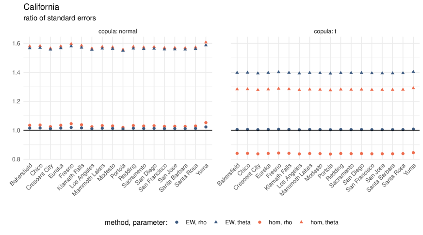
Figure 4: Separate rank-rank regression within each CZ: standard error of the indicated method divided by the correct standard error.

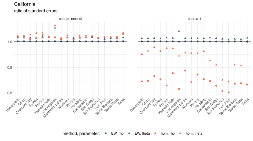
Figure 5: Rank-rank regression with clusters: standard error of the indicated method divided by the correct standard error.

For the normal copula, the hom and EW standard errors are larger than the correct one in all CZs. In the separate rank-rank regressions, for the rank-rank slope $\rho_{g}$, the ratio of standard errors is close to one, but for the expected income rank $\theta_{g,0.25}$, the ratios are close to 1.6, i.e. the hom and EW standard errors are about 60% too large. For the rank-rank regression with clusters, the ratios are all fairly close to one except for $\theta_{g,0.25}$ in Los Angeles, where the hom and EW standard errors are slightly over 5% too large.

For the t copula, on the other hand, the hom standard error for the rank-rank slope may be substantially (around 20%) smaller than the correct one. The hom standard error for the expected income rank may be around 30% too large in the separate rank-rank regressions, but up to 10% too small in the rank-rank regressions with clusters. The EW standard error may also be substantially too large (about 40% too large in the separate regressions), but is never too small.

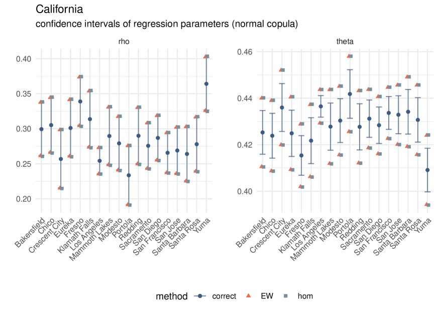
Figure 6: Separate rank-rank regression within each CZ: 95% marginal confidence intervals for the normal copula.

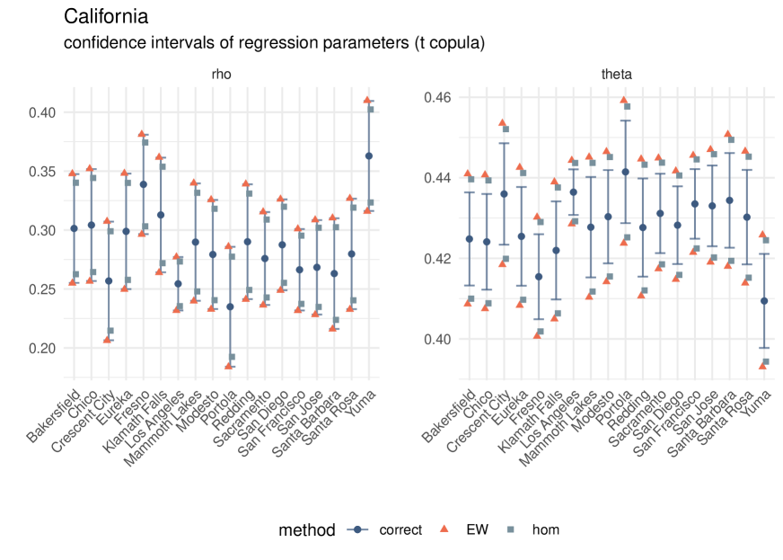
Figure 7: Separate rank-rank regression within each CZ: 95% marginal confidence intervals for the t copula.

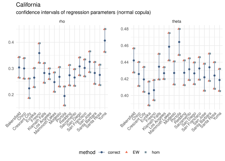
Figure 17: Rank-rank regression with clusters: 95% marginal confidence intervals for the normal copula.

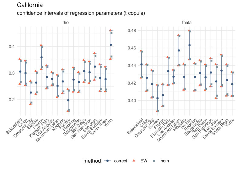
Figure 18: Rank-rank regression with clusters: 95% marginal confidence intervals for the t copula.

The differences in standard errors translate into differences in confidence intervals. Figures 6 and 7 show 95% marginal confidence intervals for the mobility estimates based on the normal and the t copulas. Figures 17 and 18 in the Appendix show the corresponding figures for the rank-rank regression with clusters.

For the normal copula, confidence intervals for the rank-rank slope are similar across the three methods. For the expected income rank, however, the confidence intervals based on hom and EW variance estimators are substantially longer than those based on the correct variance estimator, and thus lead to conservative inference. The difference in length of the hom and EW compared to the correct confidence intervals is economically meaningful in the sense that the hom and EW confidence intervals include meaningful values of mobility that the correct intervals exclude. For instance, the hom and EW confidence intervals for Modesto, San Jose, Santa Rosa, and Santa Barbara all include Italy’s (Acciari et al. (2022) report a value of 0.445) and Canada’s (Corak (2020) reports a value of 0.444) values of mobility, but the correct intervals are shorter and exclude Italy’s and Canada’s values. Similarly, Cresent City’s hom and EW confidence intervals include Australia’s value of mobility (Deutscher and Mazumder (2023) report a value of 0.45), but the correct interval is shorter and does not include Australia’s value.

For the t copula, the hom confidence intervals for the rank-rank slope are too small while the EW confidence intervals are almost identical to the correct ones. The difference in length of the hom and the correct confidence intervals is economically meaningful in the sense that the hom confidence intervals exclude meaningful values of mobility that the correct intervals include. For instance, the hom confidence intervals for Redding and Mammoth Lakes imply that mobility in these two CZs is significantly different from that in Germany (Bratberg et al. (2017) report a rank-rank slope of 0.245) and Canada (Corak (2020) report a rank-rank slope of 0.242) while the correct confidence intervals are longer and include Germany’s and Canada’s values of mobility. Similarly, Santa Barbara’s hom confidence interval implies that mobility in this CZ is significantly different from that in Norway (Bratberg et al. (2017) report a rank-rank slope of 0.223) and Italy (Acciari et al. (2022) report a rank-rank slope of 0.220), but the correct confidence interval includes Norway’s and Italy’s values of mobility.

Comparisons of mobility across countries are common in the literature (Deutscher and Mazumder (2023)) and the above discussion shows that our new confidence intervals may lead to different conclusions than those based on commonly used variance estimators.

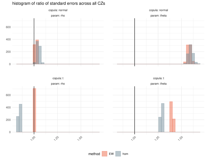
Figure 19: Rank-rank regression with clusters: histograms of ratios of standard errors.

We now turn to the set of all 709 CZs. For the separate rank-rank regressions, Figure 8 shows the histogram of ratios of standard errors across all CZs. Figure 19 in the Appendix shows the corresponding figure for the rank-rank regression with clusters. Both figures illustrate that the results for California are not special. In particular, as in California, most ratios for the normal copula and the expected income rank parameter take values around 1.6, so that most hom and EW standard errors are about 60% too large. Similarly, as in California, most hom standard errors for the t copula and the rank-rank slope are about 20% too small.

Figure 8: Separate rank-rank regression within each CZ: histograms of ratios of standard errors.

5.2 Intergenerational Mobility in the U.S. – Occupational Status

In this section, we analyze intergenerational mobility in the U.S. as in Song et al. (2020) and Ward (2022a), who measure mobility by the rank-rank relationship between fathers’ and sons’ occupational status. We focus on cohorts covered by the PSID dataset used in Ward (2022a).

Data.

We use the PSID dataset from Ward (2022a), including his construction of the Song score (not his “adjusted” Song score), the measure of occupational status.

Econometric Specification.

Our analysis deviates somewhat from that of Ward (2022a). To obtain a rank-rank regression model as in (10), we modify Ward’s regression in three ways. First, we run a rank-rank regression separately for each subpopulation of father-son pairs within which he computes ranks, i.e. within father-son birth cohort combinations. We remove father-son cohorts with fewer than 20 observations. Second, we do not use sample weights. Third, we do not average ranks over time. These three modifications to Ward (2022a)’s regression specification allow us to interpret the regression slopes as rank-rank regression slopes and the model fits into (10). We estimate the rank-rank regression with and without the covariates used by Ward (2022a). Ranks are defined as in (9) with $\omega=1$.

Results.

For the different father-son cohorts, Figure 9 shows the ratios of the hom and EW standard errors divided by the correct standard error. A ratio above (below) one means that the hom or EW standard error is larger (smaller) than the correct one. The left (right) panel reports ratios for the rank-rank regression without (with) covariates.

Some of the hom and EW standard errors are too small relative to the correct one, many are close to the correct one, but a few are substantially larger than the correct one. For instance, for the 1940-1980 father-son cohort, the hom standard error is up to 30% larger than the correct one.

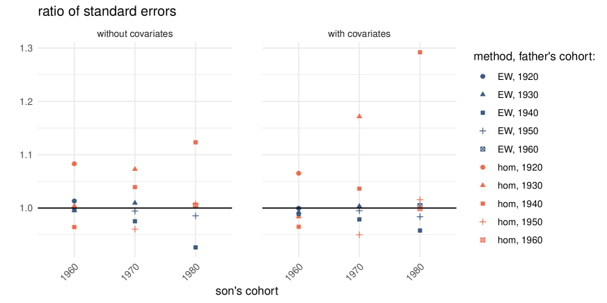
Figure 9: Standard error of the indicated method divided by the correct standard error.

The differences in standard errors translate into differences in confidence intervals for the rank-rank slope. Figure 10 shows 95% marginal confidence intervals for the rank-rank slope. Most hom and EW confidence intervals are similar to the correct confidence interval, but for the son’s cohort of 1980 we see some differences: the hom confidence sets are longer than the correct ones and lead to somewhat conservative inference.

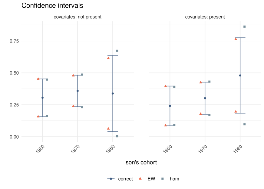
Figure 10: 95% marginal confidence intervals for the rank-rank slope.

5.3 Replication of Laboratory Experiments in Economics

In this section, we reanalyze Camerer et al. (2016) who replicated 18 laboratory experiments published in the American Economic Review and the Quarterly Journal of Economics between 2011 and 2014. Among other aspects the authors investigate how sample size and p-value in the original study relate to measures of replicability of the study. They report Spearman’s rank correlations together with indicators of these correlation’s significance (see their Figure 3).

Data.

We use the original dataset made available through the Experimental Economics Replication Project Forsell et al. (2016).

Econometric Specification.

We estimate rank-rank regressions as in (10), where $W$ only contains a constant. As in Camerer et al. (2016), we consider two different variables to play the role of $Y$ in the rank-rank regression: the sample size or the p-value in the original sample. Similarly, different variables are considered for $X$: five different measures of replicability of the study. For more information on these variables, see Camerer et al. (2016). Ranks are defined as in (9) with $\omega=1$.

Results.

Figure 11 shows the ratios of the hom and EW standard errors divided by the correct standard error. A ratio above (below) one means that the hom or EW standard error is larger (smaller) than the correct one. The left (right) panel reports ratios for the rank-rank regression with $Y$ being the p-value (sample size) in the original study.

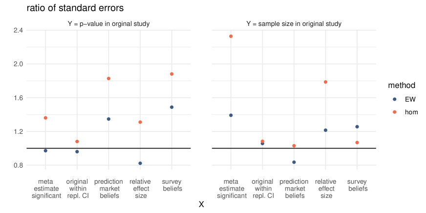
Figure 11: Standard error of the indicated method divided by the correct standard error.

Some of the hom and EW standard errors are close to, some are slightly smaller than but several are substantially larger than the correct standard errors. For instance, the hom standard error is about 2.5 times as large as the correct standard error for the measure “meta estimate significant” when $Y$ is the sample size in the original study. Several of the other hom standard errors are about twice as large as the correct one. The EW standard errors tend to be smaller than the hom standard errors, but may still be substantially larger than the correct one. Several of them are about 50% too large.

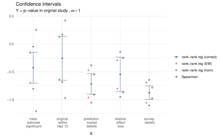
Figure 12: 95% marginal confidence intervals for the rank-rank slope and Spearman’s rank correlation.

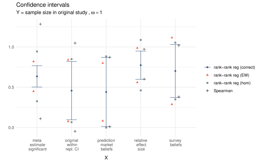
Figure 13: 95% marginal confidence intervals for the rank-rank slope and Spearman’s rank correlation.

The differences in standard errors translate into differences in confidence intervals for the rank-rank slope. Figures 12 and 13 show 95% marginal confidence intervals for the rank-rank slope for the two different outcomes. In several cases, the hom confidence interval is substantially larger than the correct confidence interval. For instance, when $Y$ is the sample size in the original study and $X$ is the measure “meta estimate significant”, the hom confidence interval is about twice as long as the correct one. The EW confidence interval is also too long, but to a lesser extent.

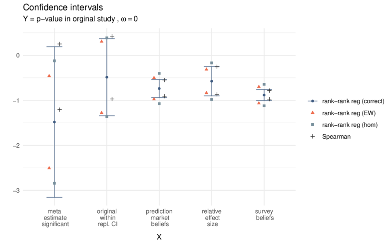
Figure 21: 95% marginal confidence intervals for the rank-rank slope and Spearman’s rank correlation.

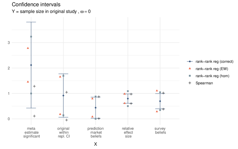
Figure 22: 95% marginal confidence intervals for the rank-rank slope and Spearman’s rank correlation.

Figures 21 and 22 in the Appendix show the confidence sets when ties are handled differently, i.e. $\omega=0$. In that case, several of the hom and EW confidence intervals are substantially shorter than the correct ones. The confidence intervals are more sensitive to the choice of how ties are handled when $X$ has fewer support points. The differences are largest for the measure “meta estimate significant”, which is a binary variable. The figures also show the confidence intervals for Spearman’s rank correlation based on Hoeffding’s theory that assumes $X$ and $Y$ have continuous marginal distributions (i.e., based on the asymptotic variance in (4)). These intervals are centered at a different value than the intervals for the rank-rank slope, illustrating the fact that pointmasses in the distributions of $X$ and/or $Y$ imply that the rank-rank slope is not equal to Spearman’s rank correlation. In addition, the confidence intervals for Spearman’s rank correlation are not valid in the presence of pointmasses.

Supplementary Appendix (For Online Publication)

Appendix A Differences in Asymptotic Variances

A.1 Asymptotic Variances as Functionals of the Copula

Under the assumption that $F$ is continuous, all three asymptotic variances analyzed in Section 2 can be written as functionals of the copula $C$. First, one can use results in Borkowf (2002) to show that

$$\sigma^{2}=144\left\{-9\theta_{1}^{2}+\theta_{2}+2\theta_{3}+2\theta_{4}+2\theta_{5}\right\}$$ (25)

where

$$\theta_{1} =\int_{0}^{1}\int_{0}^{1}uvdC(u,v)$$

$$\theta_{2} =\int_{0}^{1}\int_{0}^{1}(1-u)^{2}(1-v)^{2}dC(u,v)$$

$$\theta_{3} =\int_{0}^{1}\int_{0}^{1}\int_{0}^{1}\int_{0}^{1}(1-u-\bar{v}+C(u,\bar{v}))(1-\bar{u})(1-v)dC(u,v)dC(\bar{u},\bar{v})$$

$$\theta_{4} =\int_{0}^{1}\int_{0}^{1}\int_{0}^{1}\int_{0}^{1}\min\{1-u,1-\bar{u}\}(1-v)(1-\bar{v})dC(u,v)dC(\bar{u},\bar{v})$$

$$\theta_{5} =\int_{0}^{1}\int_{0}^{1}\int_{0}^{1}\int_{0}^{1}\min\{1-v,1-\bar{v}\}(1-u)(1-\bar{u})dC(u,v)dC(\bar{u},\bar{v})$$

Second, since $\rho=12\int_{0}^{1}\int_{0}^{1}C(u,v)dudv-3$, the homoskedastic asymptotic variance of the OLS estimator can be written as

$$\sigma_{hom}^{2}=1-\left(12\int_{0}^{1}\int_{0}^{1}C(u,v)dudv-3\right)^{2}.$$ (26)

Finally, noticing that

$$M_{kl}=\int_{0}^{1}\int_{0}^{1}(u-1/2)^{k}(v-1/2)^{l}dC(u,v),$$

it is clear that

$$\sigma_{EW}^{2}=144\left(M_{22}-2\rho M_{31}+\frac{\rho^{2}}{80}\right)$$

is a functional of $C$. Interestingly, all three variances depend on $C$, and only on $C$.

A.2 Optimizing the Difference in Variances Within Families of Copulas

This section provides details on the calculations of the maximal and minimal differences of variances presented in Figure 1. Specifically, we want to minimize and maximize the difference $\sigma_{j}^{2}-\sigma^{2}$ for $j\in\{hom,EW\}$. As shown in Appendix A.1, both variances depend on the copula $C$ of $F$, and only on $C$. To make this dependence explicit, we write $\sigma^{2}(C)$ and $\sigma_{hom}^{2}(C)$. Consider the maximization problem first. We want to solve

$$\max_{C\in\mathcal{C}}\sigma_{j}^{2}(C)-\sigma^{2}(C),$$ (27)

where $\mathcal{C}$ is a family of copulas. We consider three families, the Gaussian family, the (Student-)t family, and one with quadratic dependence.

Denote by $G_{\theta}$ the bivariate Gaussian copula with correlation $\theta$ (both variances are equal to one, means are equal to zero). The Gaussian family is then defined as

$$\mathcal{C}_{Gaussian}:=\{G_{\theta}\colon\theta\in[0,1]\}.$$

Let $T_{\theta}$ denote a (Student-)t copula with one degree of freedom and dependence parameter $\theta$. Then, the t family we consider is

$$\mathcal{C}_{t}:=\{T_{\theta}\colon\theta\in[0,1]\}.$$

Finally, consider the following “quadratic” data-generating process. $X\sim U[-1/2,1/2]$, $Y=1/2+\theta X+(1-\theta)X^{2}+\varepsilon$, where $\varepsilon\sim N(0,10^{-6})$. Denote by $F_{\theta}$ the joint distribution of $(X,Y)$ and by $Q_{\theta}$ the copula of $F_{\theta}$. Then, the quadratic family we consider is defined as

$$\mathcal{C}_{quadratic}:=\{Q_{\theta}\colon\theta\in[0,1]\}.$$

We want to solve (27) with $\mathcal{C}$ being replaced by each of the three families as well as the corresponding minimization problem. These are optimization problems in the scalar parameter $\theta\in[0,1]$, which we solve by simulation combined with a grid search. First, we define an equi-distant grid of $[0,1]$ of size 200. For each parameter value $\theta$ on this grid, we then draw $10,000$ samples of size $2,000$ from the bivariate copula in $\mathcal{C}$ with that parameter. Then, we compute the value of the objective function in (27) for each of these draws and then average over all Monte Carlo samples. Denote the maximizer $\theta$ on the grid leading to the largest value of the objective function by $\theta^{*}$. The left graph of panel A in Figure 1 then plots the magnitude of $\sigma^{2}(C_{\theta^{*}})$ (“correct”), of $\sigma^{2}_{hom}(C_{\theta^{*}})$ (“hom”) and the rank correlation $\rho$ of the copula $C_{\theta^{*}}$ in the given parametric family.

The black dots are computed as follows. In the data from Section 5.1, Los Angeles has a rank correlation of $0.254$. For each of the parametric families, we can then find the parameter value $\theta_{LA}\in[0,1]$ so that the copula from that parametric family has a rank correlation equal to $0.254$. Besides the value of $\rho$, the dots then show the values of $\sigma^{2}(C_{\theta_{LA}})$ and $\sigma^{2}_{j}(C_{\theta_{LA}})$ for $j\in\{hom,EW\}$.

The right graph in panel A of Figure 1 plots the quantities for the copula that solves the minimization problem corresponding to (27). Panel B of the figure shows the corresponding graphs for the optimization problems with $j=EW$.

Figures 14–16 show the copulas that achieve the maximum and minimum of $\sigma^{2}_{hom}(C)-\sigma^{2}(C)$ within the three families of copulas. The corresponding graphs for the EW variance look very similar and are not shown here.

Figure 14: Gaussian copulas $C$ (i.e., $C\in\mathcal{C}_{Gaussian}$) achieving the maximum and minimum of $\sigma^{2}_{hom}(C)-\sigma^{2}(C)$.

Figure 15: t copulas $C$ (i.e., $C\in\mathcal{C}_{t}$) achieving the maximum and minimum of $\sigma^{2}_{hom}(C)-\sigma^{2}(C)$.

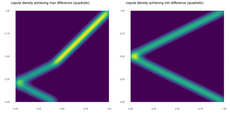
Figure 16: “Quadratic” copulas $C$ (i.e., $C\in\mathcal{C}_{quadratic}$) achieving the maximum and minimum of $\sigma^{2}_{hom}(C)-\sigma^{2}(C)$.

Appendix B Asymptotic Theory for All Regression Coefficients

B.1 Rank-Rank Regressions

In this section, we present the asymptotic theory for all coefficients in the rank-rank regression model studied in Section 3:

$$R_{Y}(Y)=\rho R_{X}(X)+W^{\prime}\beta+\varepsilon,\qquad E\left[\varepsilon\begin{pmatrix}R_{X}(X)\\ W\end{pmatrix}\right]=0,$$ (28)

where we had already introduced the equation projecting $R_{X}(X)$ onto the other regressors in $W$:

$$R_{X}(X)=W^{\prime}\gamma+\nu,\quad E[\nu W]=0.$$ (29)

To study the asymptotic behavior of the coefficients $\beta$, we now also introduce some additional projections. Let $W_{l}$ denote an element of $W:=(W_{1},\ldots,W_{p})^{\prime}$ and by $W_{-l}$ the vector of all elements of $W$ except the $l$-th. We now introduce the projection of $W_{l}$ onto $R_{X}(X)$ and the remaining regressors $W_{-l}$: for any, $l=1,\ldots,p$,

$$W_{l}=\tau_{l}R_{X}(X)+W_{-l}^{\prime}\delta_{l}+\upsilon_{l},\quad E\left[\upsilon_{l}\begin{pmatrix}R_{X}(X)\\ W_{-l}\end{pmatrix}\right]=0,$$ (30)

where $\tau_{1},\ldots,\tau_{p}$ are scalar constants and $\delta_{1},\ldots,\delta_{p}$ are $(p-1)$-dimensional vectors of constants.

Assumption 8.

For $l=1,\ldots,p$, the random variable $\upsilon_{l}$ is such that $E[\upsilon_{l}^{2}]>0$.

Consider the OLS estimator in (11):

$$\begin{pmatrix}\widehat{\rho}\\ \widehat{\beta}\end{pmatrix}=\left(\sum_{i=1}^{n}\begin{pmatrix}R_{i}^{X}\\ W_{i}\end{pmatrix}\begin{pmatrix}R_{i}^{X}&W_{i}^{\prime}\end{pmatrix}\right)^{-1}\sum_{i=1}^{n}\begin{pmatrix}R_{i}^{X}\\ W_{i}\end{pmatrix}R_{i}^{Y}.$$ (31)

Let $\sigma_{\nu}^{2}$, $h_{0,1}:=h_{1}$, $h_{0,2}:=h_{2}$, and $h_{0,3}:=h_{3}$ be as defined in Theorem 1. For $l=1,\ldots,p$, further define $\sigma_{\upsilon_{l}}^{2}:=E[\upsilon_{l}^{2}]$,

$$\phi_{0}(x,w,y) :=\frac{1}{\sigma_{\nu}^{2}}\left[h_{0,1}(x,w,y)+h_{0,2}(x,y)+h_{0,3}(x)\right]$$

$$\phi_{l}(x,y,w) :=\frac{1}{\sigma_{\upsilon_{l}}^{2}}\left[h_{l,1}(x,w,y)+h_{l,2}(x,y)+h_{l,3}(x)\right]$$

and

$$h_{l,1}(x,w,y) :=(R_{Y}(y)-\rho R_{X}(x)-w^{\prime}\beta)(w_{l}-\tau_{l}R_{X}(x)-w_{-l}^{\prime}\delta_{l}),$$

$$h_{l,2}(x,y) :=E[(I(y,Y)-\rho I(x,X)-W^{\prime}\beta)(W_{l}-\tau_{l}R_{X}(X)-W_{-l}^{\prime}\delta_{l})],$$

$$h_{l,3}(x) :=E[(R_{Y}(Y)-\rho R_{X}(X)-W^{\prime}\beta)(W_{l}-\tau_{l}I(x,X)-W_{-l}^{\prime}\delta_{l})].$$

Finally, let $\psi_{i}:=(\phi_{0}(X_{i},W_{i},Y_{i}),\phi_{1}(X_{i},W_{i},Y_{i}),\ldots,\phi_{p}(X_{i},W_{i},Y_{i}))^{\prime}$.

With the additional assumption and notation, one can derive the following joint asymptotic normality result:

Theorem 5.

Suppose that (28)–(31) hold and that Assumptions 1–3, and 8 are satisfied. Then

$$\sqrt{n}\begin{pmatrix}\widehat{\rho}-\rho\\ \widehat{\beta}-\beta\end{pmatrix}=\frac{1}{\sqrt{n}}\sum_{i=1}^{n}\psi_{i}+o_{P}(1)\to_{D}N(0,\Sigma),$$

where $\Sigma:=E[\psi_{i}\psi_{i}^{\prime}]$ and $\psi_{i}$’s are as defined above in this section.

Theorem 1 has already shown the asymptotic variance of $\widehat{\rho}$. Theorem 5 adds to that result by providing the asymptotic variance for individual components of $\widehat{\beta}$: for all $l=1,\dots,p$, we have

$$\sqrt{n}(\widehat{\beta}_{l}-\beta_{l})\to_{D}N(0,\sigma_{\beta_{l}}^{2}),$$

where

$$\sigma_{\beta_{l}}^{2}:=\frac{1}{\sigma_{\upsilon_{l}}^{4}}E\left[\left(h_{l,1}(X,W,Y)+h_{l,2}(X,Y)+h_{l,3}(X)\right)^{2}\right].$$

B.2 Rank-Rank Regressions With Clusters

In this section, we present the asymptotic theory for all coefficients in the rank-rank regression model with clusters studied in Section 4.1:

$$R_{Y}(Y)=\sum_{g=1}^{n_{G}}\mathds{1}\{G=g\}\left(\rho_{g}R_{X}(X)+W^{\prime}\beta_{g}\right)+\varepsilon,\qquad E\left[\left.\varepsilon\begin{pmatrix}R_{X}(X)\\ W\end{pmatrix}\right|G\right]=0\;\text{a.s.},$$ (32)

where we had already introduced the equation projecting $R_{X}(X)$ onto the other regressors in $W$:

$$R_{X}(X)=\sum_{g=1}^{n_{G}}\mathds{1}\{G=g\}W^{\prime}\gamma_{g}+\nu,\quad E[\left.\nu W\right|G]=0\;\text{a.s.}.$$ (33)

To study the asymptotic behavior of the coefficients $\beta_{g}$, we now also introduce some additional projections. Let $W_{l}$ denote an element of $W:=(W_{1},\ldots,W_{p})^{\prime}$ and by $W_{-l}$ the vector of all elements of $W$ except the $l$-th. We now introduce the projection of $W_{l}$ onto $R_{X}(X)$ and the remaining regressors $W_{-l}$: for any, $l=1,\ldots,p$,

$$W_{l}=\sum_{g=1}^{n_{G}}\mathds{1}\{G=g\}\left(\tau_{l,g}R_{X}(X)+W_{-l}^{\prime}\delta_{l,g}\right)+\upsilon_{l},\quad E\left[\left.\upsilon_{l}\begin{pmatrix}R_{X}(X)\\ W_{-l}\end{pmatrix}\right|G\right]=0\;\text{a.s.},$$ (34)

where $\tau_{l,g}$ are scalar constants and $\delta_{l,g}$ are $(p-1)$-dimensional vectors of constants.

Assumption 9.

For $l=1,\ldots,p$ and $g=1,\ldots,n_{G}$, the random variable $\upsilon_{l}$ is such that $E[\mathds{1}\{G=g\}\upsilon_{l}^{2}]>0$.

Consider the OLS estimator in (17):

$$\begin{pmatrix}\widehat{\rho}_{g}\\ \widehat{\beta}_{g}\end{pmatrix}=\left(\sum_{i=1}^{n}\mathds{1}\{G_{i}=c\}\begin{pmatrix}R_{i}^{X}\\ W_{i}\end{pmatrix}\begin{pmatrix}R_{i}^{X}&W_{i}^{\prime}\end{pmatrix}\right)^{-1}\sum_{i=1}^{n}\mathds{1}\{G_{i}=c\}\begin{pmatrix}R_{i}^{X}\\ W_{i}\end{pmatrix}R_{i}^{Y}.$$ (35)

Let $\sigma_{\nu,g}^{2}$, $h_{0,1,g}:=h_{1,g}$, $h_{0,2,g}:=h_{2,g}$, and $h_{0,3,g}:=h_{3,g}$ be as defined in Theorem 2. For $l=1,\ldots,p$ and $g=1,\ldots,n_{G}$, further define $\sigma_{\upsilon_{l},g}^{2}:=E[\mathds{1}\{G=g\}\upsilon_{l}^{2}]$,

$$\phi_{0,g}(\bar{g},x,w,y) :=\frac{1}{\sigma_{\nu,g}^{2}}\left[h_{0,1,g}(\bar{g},x,w,y)+h_{0,2,g}(x,y)+h_{0,3,g}(x)\right]$$

$$\phi_{l,g}(\bar{g},x,y,w) :=\frac{1}{\sigma_{\upsilon_{l},g}^{2}}\left[h_{l,1,g}(\bar{g},x,w,y)+h_{l,2,g}(x,y)+h_{l,3,g}(x)\right]$$

and

$$h_{l,1,g}(\bar{g},x,w,y) :=\mathds{1}\{\bar{g}=g\}(R_{Y}(y)-\rho_{g}R_{X}(x)-w^{\prime}\beta_{g})(w_{l}-\tau_{l,g}R_{X}(x)-w_{-l}^{\prime}\delta_{l,g}),$$

$$h_{l,2,g}(x,y) :=E[\mathds{1}\{G=g\}(I(y,Y)-\rho_{g}I(x,X)-W^{\prime}\beta_{g})(W_{l}-\tau_{l,g}R_{X}(X)-W_{-l}^{\prime}\delta_{l,g})],$$

$$h_{l,3,g}(x) :=E[\mathds{1}\{G=g\}(R_{Y}(Y)-\rho_{g}R_{X}(X)-W^{\prime}\beta_{g})(W_{l}-\tau_{l,g}I(x,X)-W_{-l}^{\prime}\delta_{l,g})].$$

Finally, let $\psi_{i,g}:=(\phi_{0,g}(G_{i},X_{i},W_{i},Y_{i}),\phi_{1,g}(G_{i},X_{i},W_{i},Y_{i}),\ldots,\phi_{p,g}(G_{i},X_{i},W_{i},Y_{i}))^{\prime}$ and $\psi_{i}:=(\phi_{0,1}(G_{i},X_{i},W_{i},Y_{i}),\ldots,\phi_{0,n_{G}}(G_{i},X_{i},W_{i},Y_{i}),\phi_{1,1}(G_{i},X_{i},W_{i},Y_{i}),\ldots,\phi_{1,n_{G}}(G_{i},X_{i},W_{i},Y_{i}),\ldots)^{\prime}$.

With the additional assumption and notation, one can derive the following joint asymptotic normality result:

Theorem 6.

Suppose (32)–(35) hold and that Assumptions 4–7, and 9 are satisfied. Then:

$$\sqrt{n}\begin{pmatrix}\widehat{\rho}-\rho\\ \widehat{\beta}-\beta\end{pmatrix}=\frac{1}{\sqrt{n}}\sum_{i=1}^{n}\psi_{i}+o_{P}(1)\to_{D}N(0,\Sigma),$$

where $\Sigma:=E[\psi_{i}\psi_{i}^{\prime}]$ and $\psi_{i}$ as defined in this section.

Theorem 2 already shows the asymptotic variance of $\widehat{\rho}_{g}$. Similarly, for the $l$-th component of $\widehat{\beta}_{g}$, denoted by $\widehat{\beta}_{l,g}$, we have

$$\sqrt{n}(\widehat{\beta}_{l,g}-\beta_{l,g})\to_{D}N(0,\sigma_{\beta_{l,g}}^{2}),$$

where

$$\sigma_{\beta_{l,g}}^{2}:=\frac{1}{\sigma_{\upsilon_{l},g}^{4}}E\left[\left(h_{l,1,g}(G,X,W,Y)+h_{l,2,g}(X,Y)+h_{l,3,g}(X)\right)^{2}\right].$$

B.3 Regression of a General Outcome on a Rank

In this section, we present the asymptotic theory for all coefficients in the rank-rank regression model studied in Section 4.2:

$$Y=\rho R_{X}(X)+W^{\prime}\beta+\varepsilon,\qquad E\left[\varepsilon\begin{pmatrix}R_{X}(X)\\ W\end{pmatrix}\right]=0,$$ (36)

with the projection equations (29) and (30). Consider the OLS estimator in (21):

$$\begin{pmatrix}\widehat{\rho}\\ \widehat{\beta}\end{pmatrix}=\left(\sum_{i=1}^{n}\begin{pmatrix}R_{i}^{X}\\ W_{i}\end{pmatrix}\begin{pmatrix}R_{i}^{X}&W_{i}^{\prime}\end{pmatrix}\right)^{-1}\sum_{i=1}^{n}\begin{pmatrix}R_{i}^{X}\\ W_{i}\end{pmatrix}Y_{i}.$$ (37)

Let $\sigma_{\nu}^{2}$, $h_{0,1}:=h_{1}$, $h_{0,2}:=h_{2}$, and $h_{0,3}:=h_{3}$ be defined as in Theorem 3. For $l=1,\ldots,p$, further define $\sigma_{\upsilon_{l}}^{2}:=E[\upsilon_{l}^{2}]$,

$$\phi_{0}(x,w,y) :=\frac{1}{\sigma_{\nu}^{2}}\left[h_{0,1}(x,w,y)+h_{0,2}(x)+h_{0,3}(x)\right]$$

$$\phi_{l}(x,y,w) :=\frac{1}{\sigma_{\upsilon_{l}}^{2}}\left[h_{l,1}(x,w,y)+h_{l,2}(x)+h_{l,3}(x)\right]$$

and

$$h_{l,1}(x,w,y) :=(y-\rho R_{X}(x)-w^{\prime}\beta)(w_{l}-\tau_{l}R_{X}(x)-w_{-l}^{\prime}\delta_{l}),$$

$$h_{l,2}(x) :=E[(Y-\rho I(x,X)-W^{\prime}\beta)(W_{l}-\tau_{l}R_{X}(X)-W_{-l}^{\prime}\delta_{l})],$$

$$h_{l,3}(x) :=E[(Y-\rho R_{X}(X)-W^{\prime}\beta)(W_{l}-\tau_{l}I(x,X)-W_{-l}^{\prime}\delta_{l})].$$

Finally, let $\psi_{i}:=(\phi_{0}(X_{i},W_{i},Y_{i}),\phi_{1}(X_{i},W_{i},Y_{i}),\ldots,\phi_{p}(X_{i},W_{i},Y_{i}))^{\prime}$.

With the additional notation, one can derive the following joint asymptotic normality result:

Theorem 7.

Suppose (29), (30), (36), and (37) hold and that Assumptions 1–3, and 8 are satisfied. Then:

$$\sqrt{n}\begin{pmatrix}\widehat{\rho}-\rho\\ \widehat{\beta}-\beta\end{pmatrix}=\frac{1}{\sqrt{n}}\sum_{i=1}^{n}\psi_{i}+o_{P}(1)\to_{D}N(0,\Sigma),$$

where $\Sigma:=E[\psi_{i}\psi_{i}^{\prime}]$ and $\psi_{i}$ as defined in this section.

Theorem 3 already shows the asymptotic variance of $\widehat{\rho}$. Similarly, for the $l$-th component of $\widehat{\beta}_{l}$ we have

$$\sqrt{n}(\widehat{\beta}_{l}-\beta_{l})\to_{D}N(0,\sigma_{\beta_{l}}^{2}),$$

where

$$\sigma_{\beta_{l}}^{2}:=\frac{1}{\sigma_{\upsilon_{l}}^{4}}E\left[\left(h_{l,1}(X,W,Y)+h_{l,2}(X,Y)+h_{l,3}(X)\right)^{2}\right].$$

Appendix C Proofs

C.1 Proofs for Section 2

Define the sample counterpart to $M_{kl}$:

$$\widehat{M}_{kl}:=\frac{1}{n}\sum_{i=1}^{n}\left(\widehat{F}_{X}(X_{i})-\frac{1}{n}\sum_{j=1}^{n}\widehat{F}_{X}(X_{j})\right)^{k}\left(\widehat{F}_{Y}(Y_{i})-\frac{1}{n}\sum_{j=1}^{n}\widehat{F}_{Y}(Y_{j})\right)^{l}.$$

Before proving Lemma 1, we state and prove the following auxiliary lemma.

Lemma 5.

Let $(X_{i},Y_{i})$, $i=1,\ldots,n$, be an i.i.d. sample from a distribution $F$ with continuous marginals. Then $\widehat{M}_{kl}=M_{kl}+o_{p}(1)$ for $(k,l)\in\{(0,2),(2,0),(2,2),(3,1),(4,0)\}$.

Proof.

Define $\widehat{P}_{Xi}:=\widehat{F}_{X}(X_{i})-\frac{1}{n}\sum_{j=1}^{n}\widehat{F}_{X}(X_{j})$, $\widetilde{P}_{Xi}:=F_{X}(X_{i})-\frac{1}{n}\sum_{j=1}^{n}F_{X}(X_{j})$, and $P_{Xi}:=F_{X}(X_{i})-E[F_{X}(X)]$. Similarly, define $\widehat{P}_{Yi}$, $\widetilde{P}_{Yi}$, and $P_{Yi}$. Also, let $R_{n}:=\max\{\sup_{x\in\mathbb{R}}|\widehat{F}_{X}(x)-F_{X}(x)|,\sup_{y\in\mathbb{R}}|\widehat{F}_{Y}(y)-F_{Y}(y)|\}$. Note that by the Glivenko-Cantelli theorem (e.g., Theorem 1.3 in Dudley (2014)), $R_{n}=o_{p}(1)$. We will use this bound, as well as the elementary identity $a^{2}-b^{2}=(a-b)^{2}+2(a-b)b$, several times without referring to them explicitly.

First, consider

$$\widehat{M}_{20} =\frac{1}{n}\sum_{i=1}^{n}\widehat{P}_{Xi}^{2}=\frac{1}{n}\sum_{i=1}^{n}\widehat{F}_{X}(X_{i})^{2}-\left(\frac{1}{n}\sum_{i=1}^{n}\widehat{F}_{X}(X_{i})\right)^{2}.$$

Using the law of large numbers, we have

$$\frac{1}{n}\sum_{i=1}^{n}\widehat{F}_{X}(X_{i})^{2}=\frac{1}{n}\sum_{i=1}^{n}F_{X}(X_{i})^{2}+\frac{1}{n}\sum_{i=1}^{n}(\widehat{F}_{X}(X_{i})^{2}-F_{X}(X_{i})^{2})$$

$$\qquad=E[F_{X}(X)^{2}]+o_{p}(1)+\frac{1}{n}\sum_{i=1}^{n}(\widehat{F}_{X}(X_{i})-F_{X}(X_{i}))^{2}+\frac{2}{n}\sum_{i=1}^{n}(\widehat{F}_{X}(X_{i})-F_{X}(X_{i}))F_{X}(X_{i})$$

$$\qquad=E[F_{X}(X)^{2}]+o_{p}(1).$$

Furthermore,

$$\left(\frac{1}{n}\sum_{i=1}^{n}\widehat{F}_{X}(X_{i})\right)^{2} =\left(\frac{1}{n}\sum_{i=1}^{n}F_{X}(X_{i})+\frac{1}{n}\sum_{i=1}^{n}(\widehat{F}_{X}(X_{i})-F_{X}(X_{i}))\right)^{2}=\left(E[F_{X}(X)]+o_{p}(1)\right)^{2}.$$

Therefore, we have shown $\widehat{M}_{20}=M_{20}+o_{p}(1)$. Analogously, $\widehat{M}_{02}=M_{02}+o_{p}(1)$.

Second, consider

$$\widehat{M}_{22} =\frac{1}{n}\sum_{i=1}^{n}\widehat{P}_{Xi}^{2}\widehat{P}_{Yi}^{2}=\frac{1}{n}\sum_{i=1}^{n}\left(\widehat{P}_{Xi}^{2}-\widetilde{P}_{Xi}^{2}\right)\widehat{P}_{Yi}^{2}+\frac{1}{n}\sum_{i=1}^{n}\left(\widehat{P}_{Yi}^{2}-\widetilde{P}_{Yi}^{2}\right)\widetilde{P}_{Xi}^{2}+\frac{1}{n}\sum_{i=1}^{n}\widetilde{P}_{Xi}^{2}\widetilde{P}_{Yi}^{2}$$

$$=:A_{n}+B_{n}+C_{n}.$$

Here,

$$A_{n} =\frac{1}{n}\sum_{i=1}^{n}\left(\widehat{P}_{Xi}^{2}-\widetilde{P}_{Xi}^{2}\right)\widehat{P}_{Yi}^{2}$$

$$=\frac{1}{n}\sum_{i=1}^{n}\left(\widehat{P}_{Xi}-\widetilde{P}_{Xi}\right)^{2}\widehat{P}_{Yi}^{2}+\frac{2}{n}\sum_{i=1}^{n}\left(\widehat{P}_{Xi}-\widetilde{P}_{Xi}\right)\widetilde{P}_{Xi}\widehat{P}_{Yi}^{2}$$

$$=\frac{1}{n}\sum_{i=1}^{n}\left(\widehat{F}_{X}(X_{i})-F_{X}(X_{i})-\frac{1}{n}\sum_{j=1}^{n}\left(\widehat{F}_{X}(X_{j})-F_{X}(X_{j})\right)\right)^{2}\widehat{P}_{Yi}^{2}$$

$$\quad+\frac{2}{n}\sum_{i=1}^{n}\left(\widehat{F}_{X}(X_{i})-F_{X}(X_{i})-\frac{1}{n}\sum_{j=1}^{n}\left(\widehat{F}_{X}(X_{j})-F_{X}(X_{j})\right)\right)\widetilde{P}_{Xi}\widehat{P}_{Yi}^{2},$$

and so

$$|A_{n}|\leq 4R_{n}^{2}\frac{1}{n}\sum_{i=1}^{n}\widehat{P}_{Yi}^{2}-2R_{n}\frac{1}{n}\sum_{i=1}^{n}\widetilde{P}_{Xi}\widehat{P}_{Yi}^{2}=o_{p}(1)$$

since $|\widehat{P}_{Yi}|\leq 1$, $|\widetilde{P}_{Xi}|\leq 1$. Also, by an analogous argument, $B_{n}=o_{p}(1)$. In addition,

$$C_{n} =\frac{1}{n}\sum_{i=1}^{n}\widetilde{P}_{Xi}^{2}\widetilde{P}_{Yi}^{2}$$

$$=\frac{1}{n}\sum_{i=1}^{n}\left(\widetilde{P}_{Xi}^{2}-P_{Xi}^{2}\right)\widetilde{P}_{Yi}^{2}+\frac{1}{n}\sum_{i=1}^{n}\left(\widetilde{P}_{Yi}^{2}-P_{Yi}^{2}\right)P_{Xi}^{2}+\frac{1}{n}\sum_{i=1}^{n}P_{Xi}^{2}P_{Yi}^{2}$$

$$=\frac{1}{n}\sum_{i=1}^{n}\left(\widetilde{P}_{Xi}-P_{Xi}\right)^{2}\widetilde{P}_{Yi}^{2}+\frac{2}{n}\sum_{i=1}^{n}\left(\widetilde{P}_{Xi}-P_{Xi}\right)P_{Xi}\widetilde{P}_{Yi}^{2}$$

$$\quad+\frac{1}{n}\sum_{i=1}^{n}\left(\widetilde{P}_{Yi}-P_{Yi}\right)^{2}P_{Xi}^{2}+\frac{2}{n}\sum_{i=1}^{n}\left(\widetilde{P}_{Yi}-P_{Yi}\right)P_{Yi}P_{Xi}^{2}+\frac{1}{n}\sum_{i=1}^{n}P_{Xi}^{2}P_{Yi}^{2}$$

$$=\frac{1}{n}\sum_{i=1}\widetilde{P}_{Yi}^{2}\left(\frac{1}{n}\sum_{j=1}^{n}\left(F_{X}(X_{j})-E(F_{X}(X))\right)\right)^{2}+\frac{2}{n}\sum_{i=1}P_{Xi}\widetilde{P}_{Yi}^{2}\left(\frac{1}{n}\sum_{j=1}^{n}\left(F_{X}(X_{j})-E(F_{X}(X))\right)\right)$$

$$\quad+\frac{1}{n}\sum_{i=1}^{n}P_{Xi}^{2}\left(\frac{1}{n}\sum_{j=1}^{n}\left(F_{Y}(Y_{j})-E(F_{Y}(Y))\right)\right)^{2}+\frac{2}{n}\sum_{i=1}^{n}P_{Yi}P_{Xi}^{2}\left(\frac{1}{n}\sum_{j=1}^{n}\left(F_{Y}(Y_{j})-E(F_{Y}(Y))\right)\right)$$

$$\quad+\frac{1}{n}\sum_{i=1}^{n}(F_{X}(X_{i})-E[F_{X}(X)])^{2}(F_{Y}(Y_{i})-E[F_{Y}(Y)])^{2}$$

$$=M_{22}+o_{p}(1)$$

by the law of large numbers and the bounds $|\widetilde{P}_{Yi}|\leq 1$, $|P_{Xi}^{2}|\leq 1$, and $|P_{Yi}|\leq 1$.

Third, consider

$$\widehat{M}_{31} =\frac{1}{n}\sum_{i=1}^{n}\widehat{P}_{Xi}^{3}\widehat{P}_{Yi}=\frac{1}{n}\sum_{i=1}^{n}\left(\widehat{P}_{Xi}^{3}-\widetilde{P}_{Xi}^{3}\right)\widehat{P}_{Yi}+\frac{1}{n}\sum_{i=1}^{n}\left(\widehat{P}_{Yi}-\widetilde{P}_{Yi}\right)\widetilde{P}_{Xi}^{3}+\frac{1}{n}\sum_{i=1}^{n}\widetilde{P}_{Xi}^{3}\widetilde{P}_{Yi}$$

$$=:D_{n}+E_{n}+F_{n}.$$

Using the elementary identity $a^{3}-b^{3}=(a-b)^{3}+3ab(a-b)$, we have

$$D_{n}=\frac{1}{n}\sum_{i=1}^{n}\left(\widehat{P}_{Xi}^{3}-\widetilde{P}_{Xi}^{3}\right)\widehat{P}_{Yi}=\frac{1}{n}\sum_{i=1}^{n}\left(\widehat{P}_{Xi}-\widetilde{P}_{Xi}\right)^{3}\widehat{P}_{Yi}+\frac{3}{n}\sum_{i=1}^{n}\left(\widehat{P}_{Xi}-\widetilde{P}_{Xi}\right)\widehat{P}_{Xi}\widetilde{P}_{Xi}\widehat{P}_{Yi}.$$

Then, continue the proof similarly as for $\widehat{M}_{22}$.

Finally, consider

$$\widehat{M}_{40} =\frac{1}{n}\sum_{i=1}^{n}\widehat{P}_{Xi}^{4}=\frac{1}{n}\sum_{i=1}^{n}\left(\widehat{P}_{Xi}^{2}-\widetilde{P}_{Xi}^{2}\right)\widehat{P}_{Xi}^{2}+\frac{1}{n}\sum_{i=1}^{n}\left(\widehat{P}_{Xi}^{2}-\widetilde{P}_{Xi}^{2}\right)\widetilde{P}_{Xi}^{2}+\frac{1}{n}\sum_{i=1}^{n}\widetilde{P}_{Xi}^{2}\widetilde{P}_{Xi}^{2}.$$

Then, continue the proof similarly as for $\widehat{M}_{22}$. ∎

Proof of Lemma 1.

Consider first the estimator for homoskedastic regression errors $\sigma_{hom}^{2}$. We have

$$\frac{1}{n}\sum_{i=1}^{n}\widehat{\varepsilon}_{i}^{2} =\frac{1}{n}\sum_{i=1}^{n}\left[R_{i}^{Y}-\bar{R}^{Y}-\widehat{\rho}(R_{i}^{X}-\bar{R}^{X})\right]^{2}$$

$$=\frac{1}{n}\sum_{i=1}^{n}(R_{i}^{Y}-\bar{R}^{Y})^{2}-\widehat{\rho}^{2}\frac{1}{n}\sum_{i=1}^{n}(R_{i}^{X}-\bar{R}^{X})^{2}$$

$$=\frac{1}{n}\sum_{i=1}^{n}\left(\widehat{F}_{Y}(Y_{i})-\frac{1}{n}\sum_{j=1}^{n}\widehat{F}_{Y}(Y_{j})\right)^{2}-\widehat{\rho}^{2}\frac{1}{n}\sum_{i=1}^{n}\left(\widehat{F}_{X}(X_{i})-\frac{1}{n}\sum_{j=1}^{n}\widehat{F}_{X}(X_{j})\right)^{2}$$

$$=\widehat{M}_{02}-\widehat{\rho}^{2}\widehat{M}_{20}=M_{02}-\rho^{2}M_{20}+o_{p}(1)=M_{02}(1-\rho^{2})+o_{p}(1)$$

where the second-to-last equality follows from Lemma 5 and the last one from noting that $M_{20}=M_{02}$. Similarly,

$$\frac{1}{n}\sum_{i=1}^{n}(R_{i}^{X}-\bar{R}^{X})^{2}=M_{02}+o_{p}(1),$$

and so (7) follows.

Next, consider the Eicker-White estimator $\sigma_{EW}^{2}$. Similarly as above, we have

$$\frac{1}{n}\sum_{i=1}^{n}\widehat{\varepsilon}_{i}^{2}(R_{i}^{X}-\bar{R}^{X})^{2} =\frac{1}{n}\sum_{i=1}^{n}\left[R_{i}^{Y}-\bar{R}^{Y}-\widehat{\rho}(R_{i}^{X}-\bar{R}^{X})\right]^{2}(R_{i}^{X}-\bar{R}^{X})^{2}$$

$$=\frac{1}{n}\sum_{i=1}^{n}(R_{i}^{Y}-\bar{R}^{Y})^{2}(R_{i}^{X}-\bar{R}^{X})^{2}$$

$$\quad-2\widehat{\rho}\frac{1}{n}\sum_{i=1}^{n}(R_{i}^{Y}-\bar{R}^{Y})(R_{i}^{X}-\bar{R}^{X})^{3}$$

$$\quad+\widehat{\rho}^{2}\frac{1}{n}\sum_{i=1}^{n}(R_{i}^{X}-\bar{R}^{X})^{4}$$

$$=\frac{1}{n}\sum_{i=1}^{n}\left(\widehat{F}_{Y}(Y_{i})-\frac{1}{n}\sum_{j=1}^{n}\widehat{F}_{Y}(Y_{j})\right)^{2}\left(\widehat{F}_{X}(X_{i})-\frac{1}{n}\sum_{j=1}^{n}\widehat{F}_{X}(X_{j})\right)^{2}$$

$$\quad-2\widehat{\rho}\frac{1}{n}\sum_{i=1}^{n}\left(\widehat{F}_{Y}(Y_{i})-\frac{1}{n}\sum_{j=1}^{n}\widehat{F}_{Y}(Y_{j})\right)\left(\widehat{F}_{X}(X_{i})-\frac{1}{n}\sum_{j=1}^{n}\widehat{F}_{X}(X_{j})\right)^{3}$$

$$\quad+\widehat{\rho}^{2}\frac{1}{n}\sum_{i=1}^{n}\left(\widehat{F}_{X}(X_{i})-\frac{1}{n}\sum_{j=1}^{n}\widehat{F}_{X}(X_{j})\right)^{4}$$

$$=\widehat{M}_{22}-2\widehat{\rho}\widehat{M}_{31}+\widehat{\rho}^{2}\widehat{M}_{40}=M_{22}-2\rho M_{31}+\rho^{2}M_{40}+o_{p}(1),$$

where the last equality follows from Lemma 5. Similarly,

$$\left(\frac{1}{n}\sum_{i=1}^{n}(R_{i}^{X}-\bar{R}^{X})^{2}\right)^{2}=M_{20}^{2}+o_{p}(1),$$

and so (8) follows by noting that $M_{20}=1/12$, and $M_{40}=1/80$. ∎

Proof of Lemma 2.

Let $a\in(0,1)$ be a constant and let $F$ be the cdf of a pair $(X,Y)$ of $U([0,1])$ random variables such that

$$Y=\begin{cases}a-X,&\text{ if }0\leq X\leq a,\\ X,&\text{ if }a<X\leq 1.\end{cases}$$

Then

$$E[\mathds{1}\{X\leq x\}Y]=\begin{cases}ax-x^{2}/2,&\text{ if }0\leq x\leq a,\\ x^{2}/2,&\text{ if }a<x\leq 1.\end{cases}$$

and

$$E[\mathds{1}\{Y\leq y\}X]=\begin{cases}ay-y^{2}/2,&\text{ if }0\leq y\leq a,\\ y^{2}/2,&\text{ if }a<y\leq 1.\end{cases}$$

Hence, given that $X>a$ if and only if $Y>a$, the function $h$ in (14) satisfies

$$E[h(X,Y)] =E\Big{[}\Big{(}X(a-X)-(aX-X^{2}/2)-(a(a-X)-(a-X)^{2}/2)\Big{)}\mathds{1}\{X\leq a\}\Big{]}$$

$$=E[-(a^{2}/2)\mathds{1}\{X\leq a\}]=-a^{3}/2$$

and

$$E[h(X,Y)^{2}] =E\left[\Big{(}X(a-X)-(aX-X^{2}/2)-(a(a-X)-(a-X)^{2}/2)\Big{)}^{2}\mathds{1}\{X\leq a\}\right]$$

$$=E[(a^{2}/2)^{2}\mathds{1}\{X\leq a\}]=a^{5}/4.$$

Therefore, given that $\sigma^{2}=144Var(h(X,Y))$ by the discussion in a remark after Theorem 1, it follows that

$$\sigma^{2}=144(E[h(X,Y)^{2}]-(E[h(X,Y)])^{2})=36(a^{5}-a^{6})$$

On the other hand, by Lemma 1,

$$\sigma^{2}_{hom} =1-\rho^{2}=1-\left(12E[XY]-3\right)^{2}=-8-144(E[XY])^{2}+72E[XY]$$

$$=-8-144\left(\frac{1}{3}-\frac{a^{3}}{6}\right)^{2}+72\left(\frac{1}{3}-\frac{a^{3}}{6}\right)=4(a^{3}-a^{6}).$$

In addition, tedious algebra shows that

$$M_{22}=\frac{1}{80}-\frac{a^{3}}{6}+\frac{a^{4}}{3}-\frac{a^{5}}{6},\quad M_{31}=\frac{1}{80}-\frac{a^{3}}{8}+\frac{a^{4}}{4}-\frac{3a^{5}}{20},\quad\rho=1-2a^{3}.$$

Thus, by Lemma 1,

$$\sigma_{EW}^{2} =144\bigg{(}\left(\frac{1}{80}-\frac{a^{3}}{6}+\frac{a^{4}}{3}-\frac{a^{5}}{6}\right)$$

$$\qquad-\left(\frac{1}{40}-\frac{3a^{3}}{10}+\frac{a^{4}}{2}-\frac{3a^{5}}{10}+\frac{a^{6}}{2}-a^{7}+\frac{3a^{8}}{5}\right)+\left(\frac{1}{80}-\frac{a^{3}}{20}+\frac{a^{6}}{20}\right)\bigg{)}$$

$$=144\left(\frac{a^{3}}{12}-\frac{a^{4}}{6}+\frac{2a^{5}}{15}-\frac{9a^{6}}{20}+a^{7}-\frac{3a^{8}}{5}\right).$$

Combining these bounds, we obtain that $\sigma^{2}_{hom}/\sigma^{2}\to\infty$ and $\sigma_{EW}^{2}/\sigma^{2}\to\infty$ as $a\to 0$, yielding the asserted claim. ∎

Proof of Lemma 3.

Let $F$ be any distribution with continuous marginals and let $(X,Y)$ be a pair of random variables with distribution $F$. Letting $F_{X}$ and $F_{Y}$ denote the corresponding marginal distributions, it follows that $U:=F_{X}(X)$ and $V:=F_{Y}(Y)$ are both $U([0,1])$ random variables. Also, $F(X,Y)=C(U,V)$, where $C$ is the copula of $F$. In addition, $\rho=Corr(F_{X}(X),F_{Y}(Y))=12E[UV]-3$.

Consider first the case $\rho\geq 0$. By Lemma 1,

$$\sigma_{hom}^{2} =1-\rho^{2}=(1-\rho)(1+\rho)\geq 1-\rho=4-12E[UV]$$

$$=4-E[12UV-6U^{2}-6V^{2}+6U^{2}+6V^{2}]$$

$$=4+6E[(U-V)^{2}]-6E[U^{2}]-6E[V^{2}]=6E[(U-V)^{2}].$$

On the other hand, by (4),

$$\sigma^{2}/9=Var\left((2U-1)(2V-1)+4\int_{0}^{1}(C(U,v)-Uv)dv+4\int_{0}^{1}(C(u,V)-uV)du\right)$$

$$\quad\leq 2E\left[\left((2U-1)(2V-1)+4\int_{0}^{1}(U\wedge v-Uv)dv+4\int_{0}^{1}(u\wedge V-uV)du-1\right)^{2}\right]$$ (38)

$$\quad\quad+2E\left[\left(4\int_{0}^{1}(C(U,v)-U\wedge v)dv+4\int_{0}^{1}(C(u,V)-u\wedge V)du\right)^{2}\right].$$ (39)

Here, observe that

$$\int_{0}^{1}(U\wedge v-Uv)dv=\frac{U-U^{2}}{2}\quad\text{and}\quad\int_{0}^{1}(u\wedge V-uV)du=\frac{V-V^{2}}{2}.$$

Thus, the expression in (38) is equal to

$$2E\left[(4UV-2U^{2}-2V^{2})^{2}\right]=8E\left[(U-V)^{4}\right]\leq 8E\left[(U-V)^{2}\right].$$

To bound (39), we claim that

$$|C(u,v)-u\wedge v|\leq P(|U-V|\geq|u-v|).$$ (40)

Indeed, if $u\leq v$, then

$$C(u,v)-u\wedge v =E[\mathds{1}\{U\leq u\}\mathds{1}\{V\leq v\}]-E[\mathds{1}\{U\leq u\}\mathds{1}\{U\leq v\}]$$

$$=E[\mathds{1}\{U\leq u\}(\mathds{1}\{V\leq v\}-\mathds{1}\{U\leq v\})]=-E[\mathds{1}\{U\leq u\}\mathds{1}\{V>v\}],$$

and so (40) follows. On the other hand, if $u>v$, then

$$C(u,v)-u\wedge v =E[\mathds{1}\{U\leq u\}\mathds{1}\{V\leq v\}]-E[\mathds{1}\{V\leq u\}\mathds{1}\{V\leq v\}]$$

$$=E[\mathds{1}\{V\leq v\}(\mathds{1}\{U\leq u\}-\mathds{1}\{V\leq u\})]=-E[\mathds{1}\{V\leq v\}\mathds{1}\{U>u\}],$$

and so (40) follows as well, yielding the claim. Thus,

$$\int_{0}^{1}|C(u,v)-u\wedge v|dv \leq\int_{0}^{1}P(|U-V|\geq|u-v|)dv$$

$$\leq 2\int_{0}^{1}P(|U-V|\geq t)dt\leq 2E[|U-V|]$$

and, similarly,

$$\int_{0}^{1}|C(u,v)-u\wedge v|du\leq 2E[|U-V|].$$

Hence, the expression in (39) is bounded from above by

$$2\times 16^{2}(E[|U-V|])^{2}\leq 512E\left[|U-V|^{2}\right].$$

Therefore, $\sigma^{2}\leq 9\times 520E[|U-V|^{2}]$, and so $\sigma^{2}_{hom}/\sigma^{2}$ is bounded below from zero.

In turn, the case $\rho<0$ can be treated similarly. The asserted claim follows. ∎

C.2 Proofs for Section 3

The proof of Theorem 1 relies on a few auxiliary results, which are presented below. As in the main text, throughout this appendix, $\omega\in[0,1]$ is fixed and the same in the definitions of $R_{X}$, $\widehat{R}_{X}$, $R_{Y}$, and $\widehat{R}_{Y}$.

Proof of Theorem 1.

By the Frisch-Waugh-Lovell theorem, the estimator $\widehat{\rho}$ in (11) can alternatively be written as

$$\widehat{\rho}=\frac{\sum_{i=1}^{n}R_{i}^{Y}(R_{i}^{X}-W_{i}^{\prime}\widehat{\gamma})}{\sum_{i=1}^{n}(R_{i}^{X}-W_{i}^{\prime}\widehat{\gamma})^{2}}=\frac{\sum_{i=1}^{n}\widehat{R}_{Y}(Y_{i})(\widehat{R}_{X}(X_{i})-W_{i}^{\prime}\widehat{\gamma})}{\sum_{i=1}^{n}(\widehat{R}_{X}(X_{i})-W_{i}^{\prime}\widehat{\gamma})^{2}},$$ (41)

where

$$\widehat{\gamma}=\left(\sum_{i=1}^{n}W_{i}W_{i}^{\prime}\right)^{-1}\left(\sum_{i=1}^{n}W_{i}\widehat{R}_{X}(X_{i})\right)$$ (42)

is the OLS estimator of a regression of $\widehat{R}_{X}(X_{i})$ on $W_{i}$. Therefore, using $\sum_{i=1}^{n}W_{i}(\widehat{R}_{X}(X_{i})-W_{i}^{\prime}\widehat{\gamma})=0$ and replacing $\widehat{R}_{Y}(Y_{i})$ in the numerator of (41) by $\widehat{R}_{Y}(Y_{i})-\rho\widehat{R}_{X}(X_{i})+\rho\widehat{R}_{X}(X_{i})$,

$$\sqrt{n}(\widehat{\rho}-\rho)=\frac{\frac{1}{\sqrt{n}}\sum_{i=1}^{n}(\widehat{R}_{Y}(Y_{i})-\rho\widehat{R}_{X}(X_{i}))(\widehat{R}_{X}(X_{i})-W_{i}^{\prime}\widehat{\gamma})}{\frac{1}{n}\sum_{i=1}^{n}(\widehat{R}_{X}(X_{i})-W_{i}^{\prime}\widehat{\gamma})^{2}}.$$ (43)

Thus, by Assumption 3 and Lemmas 9 and 10,

$$\sqrt{n}(\widehat{\rho}-\rho)=\frac{\frac{1}{\sqrt{n}}\sum_{i=1}^{n}(\widehat{R}_{Y}(Y_{i})-\rho\widehat{R}_{X}(X_{i})-W_{i}^{\prime}\beta)(\widehat{R}_{X}(X_{i})-W_{i}^{\prime}\gamma)}{\frac{1}{n}\sum_{i=1}^{n}(\widehat{R}_{X}(X_{i})-W_{i}^{\prime}\widehat{\gamma})^{2}}+o_{P}(1).$$ (44)

Consider the numerator. Define $Z_{i}:=(Y_{i},X_{i},W_{i}^{\prime})^{\prime}$ for all $i=1,\dots,n$ and

$$f(Z_{i},Z_{j},Z_{k}):=\left(I(Y_{j},Y_{i})-\rho I(X_{j},X_{i})-W_{i}^{\prime}\beta\right)(I(X_{k},X_{i})-W_{i}^{\prime}\gamma)$$

for all $i,j,k=1,\dots,n$. Also, define $h(Z_{i},Z_{j},Z_{k}):=6^{-1}\sum_{i_{1},i_{2},i_{3}}f(Z_{i_{1}},Z_{i_{2}},Z_{i_{3}})$, where the sum is over all six permutations of the triplet $(i,j,k)$, for all $i,j,k=1,\dots,n$. Note that $h$ is a symmetric function satisfying $E[h(Z_{i},Z_{j},Z_{k})]=0$ whenever $1\leq i<j<k\leq n$. Moreover, let $\Sigma_{1}$ be the set of triplets $(i,j,k)$ in $\{1,\dots,n\}^{3}$ such that all three elements are the same, $\Sigma_{2}$ be the set of triplet $(i,j,k)$ in $\{1,\dots,n\}^{3}$ such that two out of three elements are the same, and $\Sigma_{3}$ be the set of triplet $(i,j,k)$ in $\{1,\dots,n\}^{3}$ such that all three elements are different. It is then easy to check that for all $l=1,2,3$,

$$\sum_{(i,j,k)\in\Sigma_{l}}f(Z_{i},Z_{j},Z_{k})=\sum_{(i,j,k)\in\Sigma_{l}}h(Z_{i},Z_{j},Z_{k}),$$

and so

$$\sum_{i,j,k=1}^{n}f(Z_{i},Z_{j},Z_{k})=\sum_{i,j,k=1}^{n}h(Z_{i},Z_{j},Z_{k}).$$

Therefore,

$$\frac{1}{n}\sum_{i=1}^{n}(\widehat{R}_{Y}(Y_{i})-\rho\widehat{R}_{X}(X_{i})-W_{i}^{\prime}\beta)(\widehat{R}_{X}(X_{i})-W_{i}^{\prime}\gamma)$$

$$\qquad=\frac{1}{n^{3}}\sum_{i,j,k=1}^{n}\left(I(Y_{j},Y_{i})-\rho I(X_{j},X_{i})-W_{i}^{\prime}\beta\right)(I(X_{k},X_{i})-W_{i}^{\prime}\gamma)$$

$$\qquad=\frac{1}{n^{3}}\sum_{i,j,k=1}^{n}f(Z_{i},Z_{j},Z_{k})=\frac{1}{n^{3}}\sum_{i,j,k=1}^{n}h(Z_{i},Z_{j},Z_{k})$$

$$\qquad=\begin{pmatrix}n\\ 3\end{pmatrix}^{-1}\sum_{1\leq i<j<k\leq n}h(Z_{i},Z_{j},Z_{k})+o_{p}(n^{-1/2}),$$

where the last line follows from the Lemma on p. 206 of Serfling (2002), whose application is justified since $E(h(Z_{i},Z_{j},Z_{k})^{2})<\infty$ by Assumption 2. Furthermore, the results on p. 188 of Serfling (2002) imply that the U-statistic can be projected onto the basic observations. To compute the projection, note that, for $z=(y,x,w^{\prime})^{\prime}$,

$$E[f(Z_{1},Z_{2},Z_{3})\mid Z_{1}=z] =E[f(Z_{1},Z_{3},Z_{2})|Z_{1}=z]$$

$$=(R_{Y}(y)-\rho R_{X}(x)-w^{\prime}\beta)(R_{X}(x)-w^{\prime}\gamma)=h_{1}(x,w,y),$$

$$E[f(Z_{2},Z_{1},Z_{3})\mid Z_{1}=z] =E[f(Z_{3},Z_{1},Z_{2})\mid Z_{1}=z]$$

$$=E\left[(I(y,Y)-\rho I(x,X)-W^{\prime}\beta)(R_{X}(X)-W^{\prime}\gamma)\right]=h_{2}(x,y),$$

$$E[f(Z_{2},Z_{3},Z_{1})\mid Z_{i}=z] =E[f(Z_{3},Z_{2},Z_{1})\mid Z_{1}=z]$$

$$=E\left[(R_{Y}(Y)-\rho R_{X}(X)-W^{\prime}\beta)(I(x,X)-W^{\prime}\gamma)\right]=h_{3}(x).$$

Denoting $\widetilde{h}(z)=E[h(Z_{1},Z_{2},Z_{3})|Z_{1}=z]$, we thus have $\widetilde{h}(z)=(h_{1}(x,w,y)+h_{2}(x,y)+h_{3}(x))/3$, and so

$$\begin{pmatrix}n\\ 3\end{pmatrix}^{-1}\sum_{1\leq i<j<k\leq n}h(Z_{i},Z_{j},Z_{k}) =\frac{3}{n}\sum_{i=1}^{n}\widetilde{h}(Z_{i})+o_{P}(n^{-1/2})$$

$$=\frac{1}{n}\sum_{i=1}^{n}\Big{\{}h_{1}(X_{i},W_{i},Y_{i})+h_{2}(X_{i},Y_{i})+h_{3}(X_{i})\Big{\}}+o_{P}(n^{-1/2}).$$

Therefore, the central limit theorem (e.g., Theorem 9.5.6 in Dudley (2002)) implies that the numerator of (44) is asymptotically normal with mean zero and variance $E[(h_{1}(X,W,Y)+h_{2}(X,Y)+h_{3}(X))^{2}]$. By Lemma 9, the denominator of (44) converges in probability to $\sigma_{\nu}^{2}$, so that Slutsky’s lemma yields the asserted claim. ∎

Proof of Lemma 4.

First, we prove that

$$\left|\frac{1}{n}\sum_{i=1}^{n}(H_{1i}+H_{2i}+H_{3i})^{2}-\frac{1}{n}\sum_{i=1}^{n}(h_{1}(X_{i},W_{i},Y_{i})+h_{2}(X_{i},Y_{i})+h_{3}(X_{i}))^{2}\right|=o_{P}(1).$$ (45)

To do so, observe that

$$E\left[(h_{1}(X,W,Y)+h_{2}(X,Y)+h_{3}(X))^{2}\right]<\infty$$

by Assumption 2. Hence, it follows from Lemma 11 that (45) holds if

$$R_{n}:=\frac{1}{n}\sum_{i=1}^{n}(H_{1i}+H_{2i}+H_{3i}-h_{1}(X_{i},W_{i},Y_{i})-h_{2}(X_{i},Y_{i})-h_{3}(X_{i}))^{2}=o_{P}(1).$$ (46)

In turn, by the triangle inequality, $R_{n}\leq 9(R_{1n}+R_{2n}+R_{3n})$, where

$$R_{1n}:=\frac{1}{n}\sum_{i=1}^{n}(H_{1i}-h_{1}(X_{i},W_{i},Y_{i}))^{2},$$

$$R_{2n}:=\frac{1}{n}\sum_{i=1}^{n}(H_{2i}-h_{2}(X_{i},Y_{i}))^{2},$$

$$R_{3n}:=\frac{1}{n}\sum_{i=1}^{n}(H_{3i}-h_{3}(X_{i}))^{2}.$$

We bound these three terms in turn.

Regarding $R_{1n}$, we have $E[|R_{Y}(Y)-\rho R_{X}(X)-W^{\prime}\beta|^{4}]<\infty$ and $E[|R_{X}(X)-W^{\prime}\gamma|^{4}]<\infty$ by Assumption 2. Also,

$$\frac{1}{n}\sum_{i=1}^{n}\left|(R_{i}^{Y}-\widehat{\rho}R_{i}^{X}-W_{i}^{\prime}\widehat{\beta})-(R_{Y}(Y_{i})-\rho R_{X}(X_{i})-W_{i}^{\prime}\beta)\right|^{4}=o_{P}(1)$$

by Lemma 7, Theorems 1 and 5 and Assumption 2. In addition,

$$\frac{1}{n}\sum_{i=1}^{n}\left|(R_{i}^{X}-W_{i}^{\prime}\widehat{\gamma})-(R_{X}(X_{i})-W_{i}^{\prime}\gamma)\right|^{4}=o_{P}(1)$$

by Lemmas 6 and 7 and Assumption 2. Hence, $R_{1n}=o_{P}(1)$ by Lemma 12.

Regarding $R_{2n}$, we have by the triangle inequality that

$$\sqrt{R_{2n}} \leq\sup_{x,y\in\mathbb{R}}\left|\frac{1}{n}\sum_{j=1}^{n}(I(y,Y_{j})-\widehat{\rho}I(x,X_{j})-W_{j}^{\prime}\widehat{\beta})(R_{j}^{X}-W_{j}^{\prime}\widehat{\gamma})-h_{2}(x,y)\right|$$

$$\leq\sup_{x,y\in\mathbb{R}}\left|\frac{1}{n}\sum_{j=1}^{n}(I(y,Y_{j})-\widehat{\rho}I(x,X_{j})-W_{j}^{\prime}\widehat{\beta})(R_{j}^{X}-W_{j}^{\prime}\widehat{\gamma})-\widehat{h}_{2}(x,y)\right|$$

$$\quad+\sup_{x,y\in\mathbb{R}}\left|\widehat{h}_{2}(x,y)-h_{2}(x,y)\right|,$$

where

$$\widehat{h}_{2}(x,y):=\frac{1}{n}\sum_{j=1}^{n}(I(y,Y_{j})-\rho I(x,X_{j})-W_{j}^{\prime}\beta)(R_{X}(X_{j})-W_{j}^{\prime}\gamma),\quad\text{for all }x,y\in\mathbb{R}.$$

Also,

$$\sup_{x,y\in\mathbb{R}}\left|\widehat{h}_{2}(x,y)-h_{2}(x,y)\right|=o_{P}(1)$$

under Assumption 2 by Lemma 8 and the triangle inequality. In addition, for all $j=1,\dots,n$, denote

$$B_{j}(x,y):=I(y,Y_{j})-\rho I(x,X_{j})-W_{j}^{\prime}\beta,\ \widehat{B}_{j}(x,y):=I(y,Y_{j})-\widehat{\rho}I(x,X_{j})-W_{j}^{\prime}\widehat{\beta},\quad\text{for all }x,y\in\mathbb{R},$$

$$C_{j}:=R_{X}(X_{j})-W_{j}^{\prime}\gamma,\quad\widehat{C}_{j}:=R_{j}^{X}-W_{j}^{\prime}\widehat{\gamma}.$$

Then

$$\sup_{x,y\in\mathbb{R}}\frac{1}{n}\sum_{j=1}^{n}(\widehat{B}_{j}(x,y)-B_{j}(x,y))^{4}=o_{P}(1)$$

by Theorems 1 and 5 and Assumption 2;

$$\frac{1}{n}\sum_{j=1}^{n}(\widehat{C}_{j}-C_{j})^{4}=o_{P}(1)$$

by Lemmas 6 and 7 and Assumption 2;

$$\sup_{x,y\in\mathbb{R}}\frac{1}{n}\sum_{j=1}^{n}B_{j}(x,y)^{4}=O_{P}(1)\quad\text{and}\quad\frac{1}{n}\sum_{j=1}^{n}C_{j}^{4}=O_{P}(1)$$

by Assumption 2. Hence, by Lemma 12,

$$\sup_{x,y\in\mathbb{R}}\left|\frac{1}{n}\sum_{j=1}^{n}(I(y,Y_{j})-\widehat{\rho}I(x,X_{j})-W_{j}^{\prime}\widehat{\beta})(R_{j}^{X}-W_{j}^{\prime}\widehat{\gamma})-\widehat{h}_{2}(x,y)\right|$$

$$\quad=\sup_{x,y\in\mathbb{R}}\left|\frac{1}{n}\sum_{j=1}^{n}\widehat{B}_{j}(x,y)\widehat{C}_{j}-B_{j}(x,y)C_{j}\right|\leq\sup_{x,y\in\mathbb{R}}\sqrt{\frac{1}{n}\sum_{j=1}^{n}(\widehat{B}_{j}(x,y)\widehat{C}_{j}-B_{j}(x,y)C_{j})^{2}}=o_{P}(1).$$

Combining presented bounds gives $R_{2n}=o_{P}(1)$.

Regarding $R_{3n}$, we have by the triangle inequality that

$$\sqrt{R_{3n}} \leq\sup_{x\in\mathbb{R}}\left|\frac{1}{n}\sum_{j=1}^{n}(R_{j}^{Y}-\widehat{\rho}R_{j}^{X}-W_{j}^{\prime}\widehat{\beta})(I(x,X_{j})-W_{j}^{\prime}\widehat{\gamma})-h_{3}(x)\right|$$

$$\leq\sup_{x\in\mathbb{R}}\left|\frac{1}{n}\sum_{j=1}^{n}(R_{j}^{Y}-\widehat{\rho}R_{j}^{X}-W_{j}^{\prime}\widehat{\beta})(I(x,X_{j})-W_{j}^{\prime}\widehat{\gamma})-\widehat{h}_{3}(x)\right|+\sup_{x\in\mathbb{R}}|\widehat{h}_{3}(x)-h_{3}(x)|,$$

where

$$\widehat{h}_{3}(x):=\frac{1}{n}\sum_{j=1}^{n}(R_{Y}(Y_{j})-\rho R_{X}(X_{j})-W_{j}^{\prime}\beta)(I(x,X_{j})-W_{j}^{\prime}\gamma),\quad\text{for all }x\in\mathbb{R}.$$

Also,

$$\sup_{x\in\mathbb{R}}|\widehat{h}_{3}(x)-h_{3}(x)|=o_{P}(1)$$

under Assumption 2 by Lemma 8 and the triangle inequality. In addition, for all $j=1,\dots,n$, denote

$$B_{j}:=R_{Y}(Y_{j})-\rho R_{X}(X_{j})-W_{j}^{\prime}\beta,\ \widehat{B}_{j}:=R_{j}^{Y}-\widehat{\rho}R_{j}^{X}-W_{j}^{\prime}\widehat{\beta},$$

$$C_{j}(x):=I(x,X_{j})-W_{j}^{\prime}\gamma,\quad\widehat{C}_{j}(x):=I(x,X_{j})-W_{j}^{\prime}\widehat{\gamma},\quad\text{for all }x\in\mathbb{R}.$$

Then

$$\frac{1}{n}\sum_{j=1}^{n}(\widehat{B}_{j}-B_{j})^{4}=o_{P}(1)$$

by Theorems 1 and 5, Lemma 7, and Assumption 2;

$$\sup_{x\in\mathbb{R}}\frac{1}{n}\sum_{j=1}^{n}(\widehat{C}_{j}(x)-C_{j}(x))^{4}=o_{P}(1)$$

by Lemma 6 and Assumption 2;

$$\frac{1}{n}\sum_{j=1}^{n}B_{j}^{4}=O_{P}(1)\quad\text{and}\quad\sup_{x\in\mathbb{R}}\frac{1}{n}\sum_{j=1}^{n}C_{j}(x)^{4}=O_{P}(1)$$

by Assumption 2. Hence, by Lemma 12,

$$\sup_{x\in\mathbb{R}}\left|\frac{1}{n}\sum_{j=1}^{n}(R_{j}^{Y}-\widehat{\rho}R_{j}^{X}-W_{j}^{\prime}\widehat{\beta})(I(x,X_{j})-W_{j}^{\prime}\widehat{\gamma})-\widehat{h}_{3}(x)\right|$$

$$\qquad=\sup_{x\in\mathbb{R}}\left|\frac{1}{n}\sum_{j=1}^{n}\widehat{B}_{j}\widehat{C}_{j}(x)-B_{j}C_{j}(x)\right|\leq\sup_{x\in\mathbb{R}}\sqrt{\frac{1}{n}\sum_{i=1}^{n}(\widehat{B}_{j}\widehat{C}_{j}(x)-B_{j}C_{j}(x))^{2}}=o_{P}(1).$$

Combining presented bounds gives $R_{3n}=o_{P}(1)$.

Thus, (46) and hence (45) are satisfied. In turn, combining (45) with the law of large numbers yields

$$\frac{1}{n}\sum_{i=1}^{n}(H_{1i}+H_{2i}+H_{3i})^{2}\to_{P}E[(h_{1}(X,W,Y)+h_{2}(X,Y)+h_{3}(X))^{2}].$$ (47)

Also, $\widehat{\sigma}_{\nu}^{2}\to_{P}\sigma_{\nu}^{2}$ by Lemma 9. The asserted claim now follows from combining these convergence results with the continuous mapping theorem. ∎

Lemma 6.

Under Assumption 2, we have $\sqrt{n}(\widehat{\gamma}-\gamma)=O_{P}(1)$.

Proof.

By (12) and (42),

$$\sqrt{n}(\widehat{\gamma}-\gamma)=\left(\frac{1}{n}\sum_{i=1}^{n}W_{i}W_{i}^{\prime}\right)^{-1}\left(\frac{1}{\sqrt{n}}\sum_{i=1}^{n}W_{i}(\nu_{i}+\widehat{R}_{X}(X_{i})-R_{X}(X_{i}))\right).$$

By the law of large numbers and Assumption 2, $n^{-1}\sum_{i=1}^{n}W_{i}W_{i}^{\prime}\to_{P}E[WW^{\prime}]$. Also, by (12), Assumption 2, and Chebyshev’s inequality, $n^{-1/2}\sum_{i=1}^{n}W_{i}\nu_{i}=O_{P}(1)$. In addition,

$$\frac{1}{\sqrt{n}}\sum_{i=1}^{n}W_{i}(\widehat{R}_{X}(X_{i})-R_{X}(X_{i}))=\frac{1}{n^{3/2}}\sum_{i,j=1}^{n}W_{i}(I(X_{j},X_{i})-R_{X}(X_{i}))$$

$$\qquad=\frac{1}{n^{3/2}}\sum_{i=1}^{n}W_{i}(\omega-R_{X}(X_{i}))+\frac{1}{n^{3/2}}\sum_{i=1}^{n}\sum_{j\neq i}W_{i}(I(X_{j},X_{i})-R_{X}(X_{i})),$$

where $E[\|\sum_{i=1}^{n}W_{i}(\omega-R_{X}(X_{i}))\|]\leq\sum_{i=1}^{n}E[\|W_{i}\|]=O(n)$ by Assumption 2 and

$$E\left[\left\|\sum_{i=1}^{n}\sum_{j\neq i}W_{i}(I(X_{j},X_{i})-R_{X}(X_{i}))\right\|^{2}\right]=O(n^{3})$$

by Assumption 2 and results on p. 183 in Serfling (2002). Combining the presented bounds gives the asserted claim. ∎

Lemma 7.

We have $\sup_{x\in\mathbb{R}}|\widehat{R}_{X}(x)-R_{X}(x)|=o_{P}(1)$ and $\sup_{y\in\mathbb{R}}|\widehat{R}_{Y}(y)-R_{Y}(y)|=o_{P}(1)$.

Proof.

By the Glivenko-Cantelli theorem (e.g., Theorem 1.3 in Dudley (2014)), $\sup_{x\in\mathbb{R}}|\widehat{F}_{X}(x)-F_{X}(x)|=o_{P}(1)$. Also, by the Glivenko-Cantelli theorem applied to $-X_{i}$’s instead of $X_{i}$’s, $\sup_{x\in\mathbb{R}}|\widehat{F}_{X}^{-}(x)-F_{X}^{-}(x)|=o_{P}(1)$. The first claim thus follows. The second claim follows from the same argument. ∎

Lemma 8.

Under Assumption 2, we have

$$\sup_{y\in\mathbb{R}}\left|\frac{1}{n}\sum_{i=1}^{n}I(y,Y_{i})(R_{X}(X_{i})-W_{i}^{\prime}\gamma)-E[I(y,Y)(R_{X}(X)-W^{\prime}\gamma)]\right|=o_{P}(1),$$ (48)

$$\sup_{x\in\mathbb{R}}\left|\frac{1}{n}\sum_{i=1}^{n}I(x,X_{i})(R_{X}(X_{i})-W_{i}^{\prime}\gamma)-E[I(x,X)(R_{X}(X)-W^{\prime}\gamma)]\right|=o_{P}(1),$$ (49)

$$\sup_{x\in\mathbb{R}}\bigg{|}\frac{1}{n}\sum_{i=1}^{n}(R_{Y}(Y_{i})-\rho R_{X}(X_{i})-W_{i}^{\prime}\beta)I(x,X_{i})$$

$$\qquad\qquad\qquad\qquad\qquad-E[(R_{Y}(Y)-\rho R_{X}(X)-W^{\prime}\beta)I(x,X)]\bigg{|}=o_{P}(1).$$ (50)

Proof.

For any random variable $A$, let $A^{+}$ and $A^{-}$ denote $A\mathds{1}\{A\geq 0\}$ and $-A\mathds{1}\{A<0\}$, respectively. Then

$$\sup_{y\in\mathbb{R}}\left|\frac{1}{n}\sum_{i=1}^{n}I(y,Y_{i})(R_{X}(X_{i})-W_{i}^{\prime}\gamma)^{+}-E[I(y,Y)(R_{X}(X)-W^{\prime}\gamma)^{+}]\right|=o_{P}(1)$$

and

$$\sup_{y\in\mathbb{R}}\left|\frac{1}{n}\sum_{i=1}^{n}I(y,Y_{i})(R_{X}(X_{i})-W_{i}^{\prime}\gamma)^{-}-E[I(y,Y)(R_{X}(X)-W^{\prime}\gamma)^{-}]\right|=o_{P}(1)$$

by the argument parallel to that used in the proof of the Glivenko-Cantelli theorem (e.g., Theorem 1.3 in Dudley (2014)). Combining these bounds gives (48). In turn, (49) and (50) follow from the same argument. ∎

Lemma 9.

Under Assumption 2, we have

$$\frac{1}{n}\sum_{i=1}^{n}(\widehat{R}_{X}(X_{i})-W_{i}^{\prime}\widehat{\gamma})^{2}\to_{P}E[(R_{X}(X)-W^{\prime}\gamma)^{2}]=\sigma_{\nu}^{2}.$$

Proof.

By Assumption 2 and the law of large numbers,

$$\frac{1}{n}\sum_{i=1}^{n}(R_{X}(X_{i})-W_{i}^{\prime}\gamma)^{2}\to_{P}E[(R_{X}(X)-W^{\prime}\gamma)^{2}].$$

Also, using an elementary identity $a^{2}-b^{2}=(a-b)^{2}+2(a-b)b$, we have

$$\left|n^{-1}\sum_{i=1}^{n}(\widehat{R}_{X}(X_{i})-W_{i}^{\prime}\widehat{\gamma})^{2}-n^{-1}\sum_{i=1}^{n}(R_{X}(X_{i})-W_{i}^{\prime}\gamma)^{2}\right|$$

$$\qquad\leq\frac{1}{n}\sum_{i=1}^{n}(\widehat{R}_{X}(X_{i})-R_{X}(X_{i})-W_{i}^{\prime}\widehat{\gamma}+W_{i}^{\prime}\gamma)^{2}$$ (51)

$$\qquad\quad+\left|\frac{2}{n}\sum_{i=1}^{n}(\widehat{R}_{X}(X_{i})-R_{X}(X_{i})-W_{i}^{\prime}\widehat{\gamma}+W_{i}^{\prime}\gamma)(R_{X}(X_{i})-W_{i}^{\prime}\gamma)\right|.$$ (52)

The term in (51) is bounded from above by

$$\frac{2}{n}\sum_{i=1}^{n}(\widehat{R}_{X}(X_{i})-R_{X}(X_{i}))^{2}+\frac{2}{n}\sum_{i=1}^{n}(W_{i}^{\prime}\widehat{\gamma}-W_{i}^{\prime}\gamma)^{2}$$

$$\qquad\leq 2\sup_{x\in\mathbb{R}}|\widehat{R}_{X}(x)-R_{X}(x)|^{2}+2\|\widehat{\gamma}-\gamma\|^{2}\times\left\|\frac{1}{n}\sum_{i=1}^{n}W_{i}W_{i}^{\prime}\right\|=o_{P}(1)$$

by Lemmas 6 and 7 and Assumption 2. The term in (52) is bounded from above by

$$2\left(\frac{1}{n}\sum_{i=1}^{n}(\widehat{R}_{X}(X_{i})-R_{X}(X_{i})-W_{i}^{\prime}\widehat{\gamma}+W_{i}^{\prime}\gamma)^{2}\right)^{1/2}\left(\frac{1}{n}\sum_{i=1}^{n}(R_{X}(X_{i})-W_{i}^{\prime}\gamma)^{2}\right)^{1/2}=o_{P}(1)$$

by the arguments above. The asserted claim thus follows. ∎

Lemma 10.

Under Assumption 2, we have

$$\frac{1}{\sqrt{n}}\sum_{i=1}^{n}(\widehat{R}_{Y}(Y_{i})-\rho\widehat{R}_{X}(X_{i}))(\widehat{R}_{X}(X_{i})-W_{i}^{\prime}\widehat{\gamma})$$

$$\qquad=\frac{1}{\sqrt{n}}\sum_{i=1}^{n}(\widehat{R}_{Y}(Y_{i})-\rho\widehat{R}_{X}(X_{i})-W_{i}^{\prime}\beta)(\widehat{R}_{X}(X_{i})-W_{i}^{\prime}\gamma)+o_{P}(1).$$

Proof.

Using $\sum_{i=1}^{n}W_{i}(\widehat{R}_{X}(X_{i})-W_{i}^{\prime}\widehat{\gamma})=0$, we have

$$\frac{1}{\sqrt{n}}\sum_{i=1}^{n}(\widehat{R}_{Y}(Y_{i})-\rho\widehat{R}_{X}(X_{i}))(\widehat{R}_{X}(X_{i})-W_{i}^{\prime}\widehat{\gamma})$$

$$\qquad=\frac{1}{\sqrt{n}}\sum_{i=1}^{n}(\widehat{R}_{Y}(Y_{i})-\rho\widehat{R}_{X}(X_{i})-W_{i}^{\prime}\beta)(\widehat{R}_{X}(X_{i})-W_{i}^{\prime}\widehat{\gamma})$$

$$\qquad=\frac{1}{\sqrt{n}}\sum_{i=1}^{n}(\widehat{R}_{Y}(Y_{i})-\rho\widehat{R}_{X}(X_{i})-W_{i}^{\prime}\beta)(\widehat{R}_{X}(X_{i})-W_{i}^{\prime}\gamma)-R_{n}$$

where

$$R_{n}:=\frac{1}{\sqrt{n}}\sum_{i=1}^{n}(\widehat{R}_{Y}(Y_{i})-\rho\widehat{R}_{X}(X_{i})-W_{i}^{\prime}\beta)W_{i}^{\prime}(\widehat{\gamma}-\gamma)=R_{1n}+R_{2n}+R_{3n}$$

with

$$R_{1n} :=\frac{1}{\sqrt{n}}\sum_{i=1}^{n}(\widehat{R}_{Y}(Y_{i})-R_{Y}(Y_{i}))W_{i}^{\prime}(\widehat{\gamma}-\gamma)$$

$$R_{2n} :=\frac{1}{\sqrt{n}}\sum_{i=1}^{n}(\rho R_{X}(X_{i})-\rho\widehat{R}_{X}(X_{i}))W_{i}^{\prime}(\widehat{\gamma}-\gamma)$$

$$R_{3n} :=\frac{1}{\sqrt{n}}\sum_{i=1}^{n}\varepsilon_{i}W_{i}^{\prime}(\widehat{\gamma}-\gamma)$$

Consider each of these remainder terms separately. First,

$$\left|R_{1n}\right|\leq\sup_{y\in\mathbb{R}}|\widehat{R}_{Y}(y)-R_{Y}(y)|\times\frac{1}{n}\sum_{i=1}^{n}\|W_{i}\|\times\|\sqrt{n}(\widehat{\gamma}-\gamma)\|=o_{P}(1)$$

by Lemmas 6 and 7 and Assumption 2. Similarly, $|R_{2n}|=o_{P}(1)$. Finally,

$$\left|R_{3n}\right|\leq\left\|\frac{1}{n}\sum_{i=1}^{n}\varepsilon_{i}W_{i}\right\|\times\|\sqrt{n}(\widehat{\gamma}-\gamma)\|=o_{P}(1)$$

by Lemma 6, Assumption 2, and Chebyshev’s inequality. The asserted claim thus follows. ∎

Lemma 11.

For any vectors $A=(A_{1},\dots,A_{n})^{\prime}$ and $\widehat{A}=(\widehat{A}_{1},\dots,\widehat{A}_{n})^{\prime}$, we have

$$\left|\frac{1}{n}\sum_{i=1}^{n}(\widehat{A}_{i}^{2}-A_{i}^{2})\right|\leq\frac{1}{n}\sum_{i=1}^{n}(\widehat{A}_{i}-A_{i})^{2}+2\sqrt{\frac{1}{n}\sum_{i=1}^{n}(\widehat{A}_{i}-A_{i})^{2}}\sqrt{\frac{1}{n}\sum_{i=1}^{n}A_{i}^{2}}.$$

Proof.

We have

$$\left|\frac{1}{n}\sum_{i=1}^{n}(\widehat{A}_{i}^{2}-A_{i}^{2})\right| =\left|\frac{1}{n}\sum_{i=1}^{n}(\widehat{A}_{i}-A_{i})(\widehat{A}_{i}+A_{i})\right|$$

$$\leq\sqrt{\frac{1}{n}\sum_{i=1}^{n}(\widehat{A}_{i}-A_{i})^{2}}\sqrt{\frac{1}{n}\sum_{i=1}^{n}(\widehat{A}_{i}+A_{i})^{2}}$$

by the Cauchy-Schwarz inequality. Also,

$$\sqrt{\frac{1}{n}\sum_{i=1}^{n}(\widehat{A}_{i}+A_{i})^{2}}=\sqrt{\frac{1}{n}\sum_{i=1}^{n}(\widehat{A}_{i}-A_{i}+2A_{i})^{2}}\leq\sqrt{\frac{1}{n}\sum_{i=1}^{n}(\widehat{A}_{i}-A_{i})^{2}}+2\sqrt{\frac{1}{n}\sum_{i=1}^{n}A_{i}^{2}}$$

by the triangle inequality. Combining these bounds gives the asserted claim. ∎

Lemma 12.

For any vectors $B=(B_{1},\dots,B_{n})^{\prime}$, $\widehat{B}=(\widehat{B}_{1},\dots,\widehat{B}_{n})^{\prime}$, $C=(C_{1},\dots,C_{n})^{\prime}$, and $\widehat{C}=(\widehat{C}_{1},\dots,\widehat{C}_{n})^{\prime}$, we have

$$\sqrt{\frac{1}{n}\sum_{i=1}^{n}(\widehat{B}_{i}\widehat{C}_{i}-B_{i}C_{i})^{2}}\leq \left(\frac{1}{n}\sum_{i=1}^{n}(\widehat{B}_{i}-B_{i})^{4}\right)^{1/4}\left(\frac{1}{n}\sum_{i=1}^{n}(\widehat{C}_{i}-C_{i})^{4}\right)^{1/4}$$

$$+\left(\frac{1}{n}\sum_{i=1}^{n}C_{i}^{4}\right)^{1/4}\left(\frac{1}{n}\sum_{i=1}^{n}(\widehat{B}_{i}-B_{i})^{4}\right)^{1/4}$$

$$+\left(\frac{1}{n}\sum_{i=1}^{n}B_{i}^{4}\right)^{1/4}\left(\frac{1}{n}\sum_{i=1}^{n}(\widehat{C}_{i}-C_{i})^{4}\right)^{1/4}.$$

Proof.

For all $i=1,\dots,n$, we have

$$\widehat{B}_{i}\widehat{C}_{i}-B_{i}C_{i} =(\widehat{B}_{i}-B_{i})\widehat{C}_{i}+B_{i}(\widehat{C}_{i}-C_{i})$$

$$=(\widehat{B}_{i}-B_{i})(\widehat{C}_{i}-C_{i})+C_{i}(\widehat{B}_{i}-B_{i})+B_{i}(\widehat{C}_{i}-C_{i}).$$

Hence,

$$\sqrt{\frac{1}{n}\sum_{i=1}^{n}(\widehat{B}_{i}\widehat{C}_{i}-B_{i}C_{i})^{2}}\leq \sqrt{\frac{1}{n}\sum_{i=1}^{n}(\widehat{B}_{i}-B_{i})^{2}(\widehat{C}_{i}-C_{i})^{2}}$$

$$+\sqrt{\frac{1}{n}\sum_{i=1}^{n}C_{i}^{2}(\widehat{B}_{i}-B_{i})^{2}}+\sqrt{\frac{1}{n}\sum_{i=1}^{n}B_{i}^{2}(\widehat{C}_{i}-C_{i})^{2}}$$

by the triangle inequality. Applying the Cauchy-Schwarz inequality to each term on the right-hand side of this bound yields the asserted claim. ∎

C.3 Proofs for Section 4

C.3.1 Proofs for Section 4.1

Proof of Theorem 2.

Fix $g\in\{1,\dots,n_{G}\}$ and let $\widetilde{R}_{i,g}^{X}:=\mathds{1}\{G_{i}=g\}R_{i}^{X}$, $\widetilde{R}_{i,g}^{Y}:=\mathds{1}\{G_{i}=g\}R_{i}^{Y}$, and $\widetilde{W}_{i,g}:=\mathds{1}\{G_{i}=g\}W_{i}$. Then, $\widehat{\rho}_{g}$ is the OLS estimator from a regression of $\widetilde{R}_{i,g}^{Y}$ on $\widetilde{R}_{i,g}^{X}$ and $\widetilde{W}_{i,g}$ using all observations $i=1,\ldots,n$. Therefore, as in the proof of Theorem 1,

$$\sqrt{n}(\widehat{\rho}_{g}-\rho_{g}) =\frac{\frac{1}{\sqrt{n}}\sum_{i=1}^{n}\left(\widetilde{R}_{i,g}^{Y}-\rho_{g}\widetilde{R}^{X}_{i,g}\right)\left(\widetilde{R}_{i,g}^{X}-\widetilde{W}_{i,g}^{\prime}\widehat{\gamma}_{g}\right)}{\frac{1}{n}\sum_{i=1}^{n}\left(\widetilde{R}_{i,g}^{X}-\widetilde{W}_{i,g}^{\prime}\widehat{\gamma}_{g}\right)^{2}}$$

$$=\frac{\frac{1}{\sqrt{n}}\sum_{i=1}^{n}\mathds{1}\{G_{i}=g\}\left(\widehat{R}_{Y}(Y_{i})-\rho_{g}\widehat{R}_{X}(X_{i})\right)\left(\widehat{R}_{X}(X_{i})-W_{i}^{\prime}\widehat{\gamma}_{g}\right)}{\frac{1}{n}\sum_{i=1}^{n}\mathds{1}\{G_{i}=g\}\left(\widehat{R}_{X}(X_{i})-W_{i}^{\prime}\widehat{\gamma}_{g}\right)^{2}},$$

see (43). By Lemmas 13 and 14, we have

$$\sqrt{n}(\widehat{\rho}_{g}-\rho_{g})=\frac{\frac{1}{\sqrt{n}}\sum_{i=1}^{n}\mathds{1}\{G_{i}=g\}\left(\widehat{R}_{Y}(Y_{i})-\rho_{g}\widehat{R}_{X}(X_{i})-W_{i}^{\prime}\beta_{g}\right)\left(\widehat{R}_{X}(X_{i})-W_{i}^{\prime}\gamma_{g}\right)}{\frac{1}{n}\sum_{i=1}^{n}\mathds{1}\{G_{i}=g\}\left(\widehat{R}_{X}(X_{i})-W_{i}^{\prime}\widehat{\gamma}_{g}\right)^{2}}+o_{P}(1).$$ (53)

Define $Z_{i}:=(G_{i},Y_{i},X_{i},W_{i}^{\prime})^{\prime}$ for all $i=1,\dots,n$ and

$$f_{g}(Z_{i},Z_{j},Z_{k}):=\mathds{1}\{G_{i}=g\}\left(I(Y_{j},Y_{i})-\rho I(X_{j},X_{i})-W_{i}^{\prime}\beta\right)(I(X_{k},X_{i})-W_{i}^{\prime}\gamma)$$

for all $i,j,k=1,\dots,n$. Also, define $h_{g}(Z_{i},Z_{j},Z_{k}):=6^{-1}\sum_{i_{1},i_{2},i_{3}}f_{g}(Z_{i_{1}},Z_{i_{2}},Z_{i_{3}}),$ where the sum is over all six permutations $(i_{1},i_{2},i_{3})$ of the triplet $(i,j,k)$. Note that $h_{g}$ is a symmetric function satisfying $E[h_{g}(Z_{i},Z_{j},Z_{k})]=0$ whenever $1\leq i<j<k\leq n$. Also, Assumption 5 implies that $E(h_{g}(Z_{i},Z_{j},Z_{k})^{2})<\infty$. Then, letting $z:=(\bar{g},y,x,w^{\prime})^{\prime}$,

$$E[f_{g}(Z_{1},Z_{2},Z_{3})\mid Z_{1}=z] =E[f_{g}(Z_{1},Z_{3},Z_{2})|Z_{1}=z]$$

$$=\mathds{1}\{\bar{g}=g\}(R_{Y}(y)-\rho_{g}R_{X}(x)-w^{\prime}\beta_{g})(R_{X}(x)-w^{\prime}\gamma_{g})$$

$$=h_{1,g}(\bar{g},x,w,y),$$

$$E[f_{g}(Z_{2},Z_{1},Z_{3})\mid Z_{1}=z] =E[f_{g}(Z_{3},Z_{1},Z_{2})\mid Z_{1}=z]$$

$$=E\left[\mathds{1}\{G=g\}(I(y,Y)-\rho_{g}I(x,X)-W^{\prime}\beta_{g})(R_{X}(X)-W^{\prime}\gamma_{g})\right]$$

$$=h_{2,g}(x,y),$$

$$E[f_{g}(Z_{2},Z_{3},Z_{1})\mid Z_{i}=z] =E[f_{g}(Z_{3},Z_{2},Z_{1})\mid Z_{1}=z]$$

$$=E\left[\mathds{1}\{G=g\}(R_{Y}(Y)-\rho_{g}R_{X}(X)-W^{\prime}\beta_{g})(I(x,X)-W^{\prime}\gamma_{g})\right]$$

$$=h_{3,g}(x),$$

we can argue as in the proof of Theorem 1 that

$$\frac{1}{n}\sum_{i=1}^{n}\mathds{1}\{G_{i}=g\}\left(\widehat{R}_{Y}(Y_{i})-\rho_{g}\widehat{R}_{X}(X_{i})-W_{i}^{\prime}\beta_{g}\right)\left(\widehat{R}_{X}(X_{i})-W_{i}^{\prime}\gamma_{g}\right)\\ =\frac{1}{n}\sum_{i=1}^{n}\Big{\{}h_{1,g}(X_{i},W_{i},Y_{i})+h_{2,g}(X_{i},Y_{i})+h_{3,g}(X_{i})\Big{\}}+o_{P}(n^{-1/2}).$$

The remainder of the proof then follows that of Theorem 1. ∎

Lemma 13.

Under Assumption 5, we have for any $g=1,\ldots,n_{G}$,

$$n^{-1}\sum_{i=1}^{n}\mathds{1}\{G_{i}=g\}(\widehat{R}_{X}(X_{i})-W_{i}^{\prime}\widehat{\gamma}_{g})^{2}\to_{P}E[\mathds{1}\{G_{i}=g\}(R_{X}(X)-W^{\prime}\gamma_{g})^{2}]=\sigma_{\nu,g}^{2}.$$

Proof.

Similar to that of Lemma 9. ∎

Lemma 14.

Under Assumption 5, we have for any $g=1,\ldots,n_{G}$,

$$\frac{1}{\sqrt{n}}\sum_{i=1}^{n}\mathds{1}\{G_{i}=g\}(\widehat{R}_{Y}(Y_{i})-\rho_{g}\widehat{R}_{X}(X_{i}))(\widehat{R}_{X}(X_{i})-W_{i}^{\prime}\widehat{\gamma}_{g})$$

$$\qquad=\frac{1}{\sqrt{n}}\sum_{i=1}^{n}\mathds{1}\{G_{i}=g\}(\widehat{R}_{Y}(Y_{i})-\rho_{g}\widehat{R}_{X}(X_{i})-W_{i}^{\prime}\beta_{g})(\widehat{R}_{X}(X_{i})-W_{i}^{\prime}\gamma_{g})+o_{P}(1).$$

Proof.

Similar to that of Lemma 10. ∎

C.3.2 Proofs for Section 4.2

Proof of Theorem 3.

As in the proof of Theorem 1,

$$\sqrt{n}(\widehat{\rho}-\rho)=\frac{\frac{1}{\sqrt{n}}\sum_{i=1}^{n}(Y_{i}-\rho\widehat{R}_{X}(X_{i}))(\widehat{R}_{X}(X_{i})-W_{i}^{\prime}\widehat{\gamma})}{\frac{1}{n}\sum_{i=1}^{n}(\widehat{R}_{X}(X_{i})-W_{i}^{\prime}\widehat{\gamma})^{2}}.$$

By Lemmas 9 and 15, we have

$$\sqrt{n}(\widehat{\rho}-\rho)=\frac{\frac{1}{\sqrt{n}}\sum_{i=1}^{n}(Y_{i}-\rho\widehat{R}_{X}(X_{i})-W_{i}^{\prime}\beta)(\widehat{R}_{X}(X_{i})-W_{i}^{\prime}\gamma)}{\frac{1}{n}\sum_{i=1}^{n}(\widehat{R}_{X}(X_{i})-W_{i}^{\prime}\widehat{\gamma})^{2}}+o_{P}(1).$$ (54)

Define $Z_{i}:=(Y_{i},X_{i},W_{i}^{\prime})^{\prime}$ for all $i=1,\dots,n$ and

$$f(Z_{i},Z_{j},Z_{k}):=\left(Y_{i}-\rho I(X_{j},X_{i})-W_{i}^{\prime}\beta\right)(I(X_{k},X_{i})-W_{i}^{\prime}\gamma)$$

for all $i,j,k=1,\dots,n$. Also, define $h(Z_{i},Z_{j},Z_{k}):=6^{-1}\sum_{i_{1},i_{2},i_{3}}f(Z_{i_{1}},Z_{i_{2}},Z_{i_{3}}),$ where the sum is taken over all six permutations $(i_{1},i_{2},i_{3})$ of the triplet $(i,j,k)$. Since $E[\varepsilon^{4}]<\infty$ and Assumption 2 imply $E[h(Z_{i},Z_{j},Z_{k})^{2}]<\infty$, we can argue as in the proof of Theorem 1 to show that

$$\frac{1}{n}\sum_{i=1}^{n}(Y_{i}-\rho\widehat{R}_{X}(X_{i})-W_{i}^{\prime}\beta)(\widehat{R}_{X}(X_{i})-W_{i}^{\prime}\gamma)\\ =\frac{1}{n}\sum_{i=1}^{n}\Big{\{}h_{1}(X_{i},W_{i},Y_{i})+h_{2}(X_{i})+h_{3}(X_{i})\Big{\}}+o_{P}(n^{-1/2})$$ (55)

where for $z=(x,y,w^{\prime})^{\prime}$, we define

$$E[f(Z_{i},Z_{j},Z_{k})\mid Z_{i}=z] =E[f(Z_{i},Z_{k},Z_{j})|Z_{i}=z]$$

$$=(y-\rho R_{X}(x)-w^{\prime}\beta)(R_{X}(x)-w^{\prime}\gamma)=h_{1}(x,w,y),$$

$$E[f(Z_{j},Z_{i},Z_{k})\mid Z_{i}=z] =E[f(Z_{k},Z_{i},Z_{j})\mid Z_{i}=z]$$

$$=E\left[(Y-\rho I(x,X)-W^{\prime}\beta)(R_{X}(X)-W^{\prime}\gamma)\right]=h_{2}(x),$$

$$E[f(Z_{j},Z_{k},Z_{i})\mid Z_{i}=z] =E[f(Z_{k},Z_{j},Z_{i})\mid Z_{i}=z]$$

$$=E\left[(Y-\rho R_{X}(X)-W^{\prime}\beta)(I(x,X)-W^{\prime}\gamma)\right]=h_{3}(x)$$

Combining (54) with (55) then implies the desired result by the same argument as that in the proof of Theorem 1. ∎

Lemma 15.

Under Assumption 2, we have

$$\frac{1}{\sqrt{n}}\sum_{i=1}^{n}(Y_{i}-\rho\widehat{R}_{X}(X_{i}))(\widehat{R}_{X}(X_{i})-W_{i}^{\prime}\widehat{\gamma})$$

$$\qquad=\frac{1}{\sqrt{n}}\sum_{i=1}^{n}(Y_{i}-\rho\widehat{R}_{X}(X_{i})-W_{i}^{\prime}\beta)(\widehat{R}_{X}(X_{i})-W_{i}^{\prime}\gamma)+o_{P}(1).$$

Proof.

Using $\sum_{i=1}^{n}W_{i}(\widehat{R}_{X}(X_{i})-W_{i}^{\prime}\widehat{\gamma})=0$, we have

$$\frac{1}{\sqrt{n}}\sum_{i=1}^{n}(Y_{i}-\rho\widehat{R}_{X}(X_{i}))(\widehat{R}_{X}(X_{i})-W_{i}^{\prime}\widehat{\gamma})$$

$$\qquad=\frac{1}{\sqrt{n}}\sum_{i=1}^{n}(Y_{i}-\rho\widehat{R}_{X}(X_{i})-W_{i}^{\prime}\beta)(\widehat{R}_{X}(X_{i})-W_{i}^{\prime}\widehat{\gamma})$$

$$\qquad=\frac{1}{\sqrt{n}}\sum_{i=1}^{n}(Y_{i}-\rho\widehat{R}_{X}(X_{i})-W_{i}^{\prime}\beta)(\widehat{R}_{X}(X_{i})-W_{i}^{\prime}\gamma)-R_{n}$$

where

$$R_{n}:=\frac{1}{\sqrt{n}}\sum_{i=1}^{n}(Y_{i}-\rho\widehat{R}_{X}(X_{i})-W_{i}^{\prime}\beta)W_{i}^{\prime}(\widehat{\gamma}-\gamma)=R_{1n}+R_{2n}$$

with

$$R_{1n} :=\frac{1}{\sqrt{n}}\sum_{i=1}^{n}\varepsilon_{i}W_{i}^{\prime}(\widehat{\gamma}-\gamma)$$

$$R_{2n} :=\frac{1}{\sqrt{n}}\sum_{i=1}^{n}(\rho R_{X}(X_{i})-\rho\widehat{R}_{X}(X_{i}))W_{i}^{\prime}(\widehat{\gamma}-\gamma)$$

By the same arguments as in the proof of Lemma 10, we have $|R_{1n}|=o_{P}(1)$ and $|R_{2n}|=o_{P}(1)$ and the desired result follows. ∎

C.3.3 Proofs for Section 4.3

Proof of Theorem 4.

As in the proof of Theorem 1,

$$\sqrt{n}(\widehat{\beta}_{l}-\beta_{l})=\frac{\frac{1}{\sqrt{n}}\sum_{i=1}^{n}(\widehat{R}_{Y}(Y_{i})-\beta_{l}W_{l,i})(W_{l,i}-W_{-l,i}^{\prime}\widehat{\gamma}_{l})}{\frac{1}{n}\sum_{i=1}^{n}(W_{l,i}-W_{-l,i}^{\prime}\widehat{\gamma}_{l})^{2}}$$

with

$$\widehat{\gamma}=\left(\sum_{i=1}^{n}W_{-l,i}W_{-l,i}^{\prime}\right)^{-1}\left(\sum_{i=1}^{n}W_{-l,i}W_{l,i}\right).$$

By Lemmas 16 and 17, we have

$$\sqrt{n}(\widehat{\beta}_{l}-\beta_{l})=\frac{\frac{1}{\sqrt{n}}\sum_{i=1}^{n}(\widehat{R}_{Y}(Y_{i})-W_{i}^{\prime}\beta)(W_{l,i}-W_{-l,i}^{\prime}\gamma_{l})}{\frac{1}{n}\sum_{i=1}^{n}(W_{l,i}-W_{-l,i}^{\prime}\widehat{\gamma}_{l})^{2}}+o_{P}(1).$$ (56)

Define $Z_{i}:=(Y_{i},W_{i}^{\prime})^{\prime}$ for all $i=1,\dots,n$,

$$f(Z_{i},Z_{j}):=\left(I(Y_{j},Y_{i})-W_{i}^{\prime}\beta\right)(W_{l,i}-W_{-l,i}^{\prime}\gamma_{l})$$

for all $i,j=1,\dots,n$, and $h(Z_{i},Z_{j}):=2^{-1}(f(Z_{i},Z_{j})+f(Z_{j},Z_{i}))$ for all $i,j=1,\dots,n$. Since Assumption 2 implies $E[h(Z_{i},Z_{j})^{2}]<\infty$, we can argue as in the proof of Theorem 1 that

$$\frac{1}{n}\sum_{i=1}^{n}(\widehat{R}_{Y}(Y_{i})-W_{i}^{\prime}\beta)(W_{l,i}-W_{-l,i}^{\prime}\gamma_{l})=\frac{1}{n}\sum_{i=1}^{n}\Big{\{}h_{l,1}(W_{i},Y_{i})+h_{l,2}(Y_{i})\Big{\}}+o_{P}(n^{-1/2})$$ (57)

where for $z=(y,w^{\prime})^{\prime}$, we define

$$E[f(Z_{i},Z_{j})\mid Z_{i}=z] =(R_{Y}(y)-w^{\prime}\beta)(w_{l}-w_{-l}^{\prime}\gamma_{l})=h_{l,1}(w,y),$$

$$E[f(Z_{j},Z_{i})\mid Z_{i}=z] =E\left[(I(y,Y)-W^{\prime}\beta)(W_{l}-W_{-l}^{\prime}\gamma_{l})\right]=h_{l,2}(y).$$

Combining (56) with (57) then implies the desired result by the same argument as that in the proof of Theorem 1. ∎

Lemma 16.

Under Assumption 2, for each $l=1,\ldots,p$, we have $\sigma_{\nu_{l}}^{2}>0$ and

$$n^{-1}\sum_{i=1}^{n}(W_{l,i}-W_{-l,i}^{\prime}\widehat{\gamma}_{l})^{2}\to_{P}E[(W_{l}-W_{-l}^{\prime}\gamma_{l})^{2}]=\sigma_{\nu_{l}}^{2}.$$

Proof.

Since it follows from Assumption 2 that $\sigma_{\nu_{l}}^{2}>0$, the proof is similar to that of Lemma 9. ∎

Lemma 17.

Under Assumption 2, for each $l=1,\ldots,p$, we have

$$\frac{1}{\sqrt{n}}\sum_{i=1}^{n}(\widehat{R}_{Y}(Y_{i})-\beta_{l}W_{l,i})(W_{l,i}-W_{-l,i}^{\prime}\widehat{\gamma}_{l})=\frac{1}{\sqrt{n}}\sum_{i=1}^{n}(\widehat{R}_{Y}(Y_{i})-W_{i}^{\prime}\beta)(W_{l,i}-W_{-l,i}^{\prime}\gamma_{l})+o_{P}(1).$$

Proof.

Similar to that of Lemma 10. ∎

C.4 Proofs for Appendix B

Proof of Theorem 5.

Fix $l=1,\dots,p$. As in the proof of Theorem 1,

$$\sqrt{n}(\widehat{\beta}_{l}-\beta_{l})=\frac{\frac{1}{\sqrt{n}}\sum_{i=1}^{n}(\widehat{R}_{Y}(Y_{i})-\beta_{l}W_{l,i})(W_{l,i}-\widehat{\tau}_{l}\widehat{R}_{X}(X_{i})-W_{-l,i}^{\prime}\widehat{\delta}_{l})}{\frac{1}{n}\sum_{i=1}^{n}(W_{l,i}-\widehat{\tau}_{l}\widehat{R}_{X}(X_{i})-W_{-l,i}^{\prime}\widehat{\delta}_{l})^{2}},$$

where

$$\begin{pmatrix}\widehat{\tau_{l}}\\ \widehat{\delta_{l}}\end{pmatrix}=\left(\sum_{i=1}^{n}\begin{pmatrix}\widehat{R}_{X}(X_{i})\\ W_{-l,i}\end{pmatrix}\begin{pmatrix}\widehat{R}_{X}(X_{i})&W_{-l,i}^{\prime}\end{pmatrix}\right)^{-1}\sum_{i=1}^{n}\begin{pmatrix}\widehat{R}_{X}(X_{i})\\ W_{-l,i}\end{pmatrix}W_{l,i}.$$

Further, again by the same arguments as those in the proof of Theorem 1,

$$\frac{1}{\sqrt{n}}\sum_{i=1}^{n}(\widehat{R}_{Y}(Y_{i})-\beta_{l}W_{l,i})(W_{l,i}-\widehat{\tau}_{l}\widehat{R}_{X}(X_{i})-W_{-l,i}^{\prime}\widehat{\delta}_{l})$$

$$\qquad=\frac{1}{\sqrt{n}}\sum_{i=1}^{n}(\widehat{R}_{Y}(Y_{i})-\rho\widehat{R}_{X}(X_{i})-W_{i}^{\prime}\beta)(W_{l,i}-\tau_{l}\widehat{R}_{X}(X_{i})-W_{-l,i}^{\prime}\delta_{l})+o_{P}(1)$$

$$\qquad=\frac{1}{\sqrt{n}}\sum_{i=1}^{n}\Big{\{}h_{l,1}(X_{i},W_{i},Y_{i})+h_{l,2}(X_{i},Y_{i})+h_{l,3}(X_{i})\Big{\}}+o_{P}(1)$$

and

$$\frac{1}{n}\sum_{i=1}^{n}(W_{l,i}-\widehat{\tau}_{l}\widehat{R}_{X}(X_{i})-W_{-l,i}^{\prime}\widehat{\delta}_{l})^{2}\to_{P}\sigma_{v_{l}}^{2}.$$

Combining these results with the central limit theorem and Slutsky’s lemma gives the asserted claim. ∎

Proof of Theorem 6.

Similar to that of Theorem 2, based on the same relationship as that between Theorem 5 and Theorem 1. ∎

Proof of Theorem 7.

Similar to that of Theorem 3, based on the same relationship as that between Theorem 5 and Theorem 1. ∎

Appendix D Additional Results for the Empirical Applications

D.1 Intergenerational Mobility in the U.S. – Income

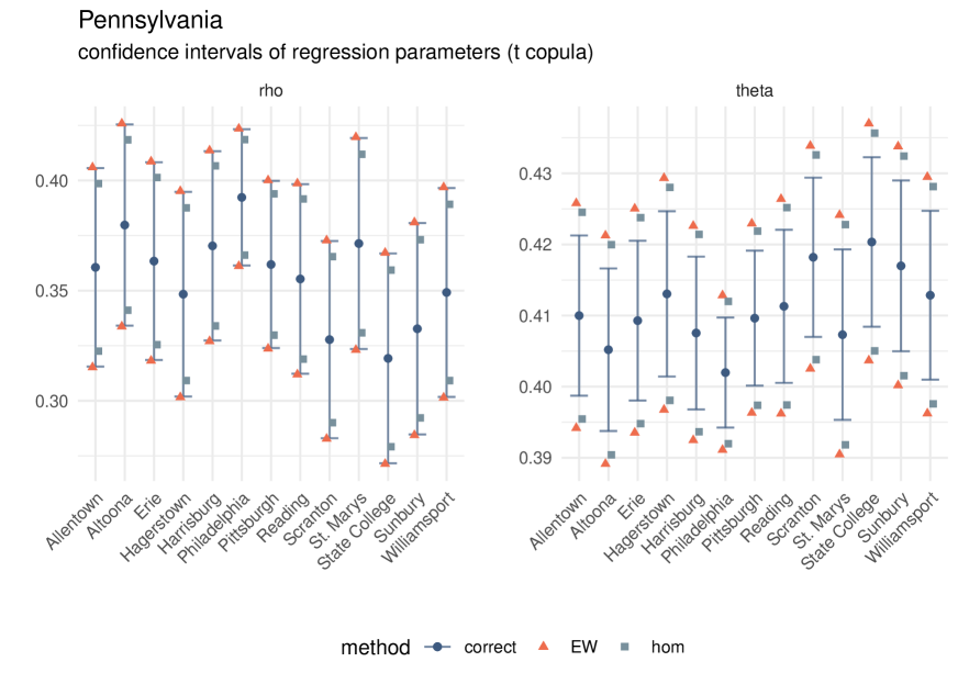
Figure 20: Separate rank-rank regression within each CZ: 95% marginal confidence intervals for the t copula.

D.2 Replication of Laboratory Experiments in Economics

References

- (1)
- Acciari et al. (2022) Acciari, P., A. Polo, and G. L. Violante (2022): “And Yet It Moves: Intergenerational Mobility in Italy,” American Economic Journal: Applied Economics, 14, 118–63.
- Bickel and Freedman (1981) Bickel, P., and D. Freedman (1981): “Some asymptotic theory for the bootstrap,” Annals of Statistics, 9, 1196–1217.
- Borkowf (2002) Borkowf, C. B. (2002): “Computing the nonnull asymptotic variance and the asymptotic relative efficiency of Spearman’s rank correlation,” Computational Statistics & Data Analysis, 39, 271–286.
- Bratberg et al. (2017) Bratberg, E., J. Davis, B. Mazumder, M. Nybom, D. D. Schnitzlein, and K. Vaage (2017): “A Comparison of Intergenerational Mobility Curves in Germany, Norway, Sweden, and the US,” The Scandinavian Journal of Economics, 119, 72–101.
- Camerer et al. (2016) Camerer, C. F., A. Dreber, E. Forsell et al. (2016): “Evaluating replicability of laboratory experiments in economics,” Science, 351, 1433–1436.
- Carneiro et al. (2023) Carneiro, P., Y. Cruz Aguayo, F. Salvati, and N. Schady (2023): “The effect of classroom rank on learning throughout elementary school: experimental evidence from Ecuador,” Working Paper CWP19/23, CeMMAP.
- Chatterjee (2023) Chatterjee, S. (2023): “A survey of some recent developments in measures of association,” arXiv:2211.04702.
- Chernozhukov et al. (2022) Chernozhukov, V., J. Escanciano, H. Ichimura, W. Newey, and J. Robins (2022): “Locally robust semiparametric estimation,” Econometrica, 90, 1501–1535.
- Chetty et al. (2022a) Chetty, R., J. Friedman, N. Hendren, M. R. Jones, and S. R. Porter (2022a): “Replication Data for: The Opportunity Atlas: Mapping the Childhood Roots of Social Mobility,” https://doi.org/10.7910/DVN/NKCQM1.
- Chetty et al. (2018) Chetty, R., J. N. Friedman, N. Hendren, M. R. Jones, and S. R. Porter (2018): “The Opportunity Atlas: Mapping the Childhood Roots of Social Mobility,” Working Paper 25147, NBER.
- Chetty et al. (2011) Chetty, R., J. N. Friedman, N. Hilger, E. Saez, D. W. Schanzenbach, and D. Yagan (2011): “How Does Your Kindergarten Classroom Affect Your Earnings? Evidence from Project Star,” The Quarterly Journal of Economics, 126, 1593–1660.
- Chetty and Hendren (2018) Chetty, R., and N. Hendren (2018): “The Impacts of Neighborhoods on Intergenerational Mobility I: Childhood Exposure Effects,” The Quarterly Journal of Economics, 133, 1107–1162.
- Chetty et al. (2014) Chetty, R., N. Hendren, P. Kline, and E. Saez (2014): “Where is the land of Opportunity? The Geography of Intergenerational Mobility in the United States,” The Quarterly Journal of Economics, 129, 1553.
- Chetty et al. (2022b) (2022b): “Replication Data for: Where is the Land of Opportunity? The Geography of Intergenerational Mobility in the United States,” https://doi.org/10.7910/DVN/NALG3E.
- Corak (2020) Corak, M. (2020): “The Canadian Geography of Intergenerational Income Mobility,” The Economic Journal, 130, 2134–2174.
- de la Croix and Goni (2022) de la Croix, D., and M. Goni (2022): “Nepotism vs. Intergenerational Transmission of Human Capital in Academia (1088–1800),” discussion paper.
- Dahl and DeLeire (2008) Dahl, M., and T. DeLeire (2008): “The Association between Children’s Earnings and Fathers’ Lifetime Earnings: Estimates Using Administrative Data,” Discussion Paper 1342-08, Institute for Research on Poverty.
- Deutscher and Mazumder (2023) Deutscher, N., and B. Mazumder (2023): “Measuring Intergenerational Income Mobility: A Synthesis of Approaches,” Journal of Economic Literature, 61, 988–1036.
- Dudley (2002) Dudley, R. M. (2002): Real Analysis and Probability, Cambridge Studies in Advanced Mathematics: Cambridge University Press, 2nd edition.
- Dudley (2014) (2014): Uniform Central Limit Theorems: Cambridge University Press, Cambridge.
- Fang and Santos (2019) Fang, Z., and A. Santos (2019): “Inference on directionally differentiable functions,” Review of Economc Studies, 86, 377–412.
- Forsell et al. (2016) Forsell, E., M. Johannesson, C. Camerer et al. (2016): “Experimental Economics Replication Project,” osf.io/bzm54, Jun.
- Genest et al. (2013) Genest, C., J. Nes̆lehova, and B. Rémillard (2013): “On the estimation of Spearman’s rho and related tests of independence for possibly discontinuous multivariate data,” Journal of Multivariate Analysis, 98, 214–228.
- Hoeffding (1948) Hoeffding, W. (1948): “A Class of Statistics with Asymptotically Normal Distribution,” The Annals of Mathematical Statistics, 19, 293 – 325.
- Klein et al. (2020) Klein, M., T. Wright, and J. Wieczorek (2020): “A joint confidence region for an overall ranking of populations,” Journal of the Royal Statistical Society: Series C (Applied Statistics), 69, 589–606.
- Mesfioui and Quessy (2010) Mesfioui, M., and J.-F. Quessy (2010): “Concordance measures for multivariate non-continuous random vectors,” Journal of Multivariate Analysis, 101, 2398–2410.
- Mogstad et al. (2023) Mogstad, M., J. P. Romano, A. M. Shaikh, and D. Wilhelm (2023): “Inference for Ranks with Applications to Mobility across Neighbourhoods and Academic Achievement across Countries,” The Review of Economic Studies, forthcoming.
- Mogstad and Torsvik (2023) Mogstad, M., and G. Torsvik (2023): “Family background, neighborhoods, and intergenerational mobility,” in Handbook of the Economics of the Family, Volume 1 ed. by Lundberg, S., and Voena, A. Volume 1 of Handbook of the Economics of the Family: North-Holland, Chap. 6, 327–387.
- Murphy and Weinhardt (2020) Murphy, R., and F. Weinhardt (2020): “Top of the Class: The Importance of Ordinal Rank,” The Review of Economic Studies, 87, 2777–2826.
- Nes̆lehova (2007) Nes̆lehova, J. (2007): “On rank correlation measures for non-continuous random variables,” Journal of Multivariate Analysis, 98, 544–567.
- Newey (1994) Newey, W. (1994): “The asymptotic variance of semiparametric estimators,” Econometrica, 62, 1349–1382.
- Ornstein and Lyhagen (2016) Ornstein, P., and J. Lyhagen (2016): “Asymptotic properties of Spearman’s rank correlation for variables with finite support,” PLOS one, 11, 1–7.
- Serfling (2002) Serfling, R. J. (2002): Approximation Theorems of Mathematical Statistics: John Wiley & Sons, Inc.
- Sharkey and Torrats-Espinosa (2017) Sharkey, P., and G. Torrats-Espinosa (2017): “The effect of violent crime on economic mobility,” Journal of Urban Economics, 102, 22–33.
- Song et al. (2020) Song, X., C. G. Massey, K. A. Rolf, J. P. Ferrie, J. L. Rothbaum, and Y. Xie (2020): “Long-term decline in intergenerational mobility in the United States since the 1850s,” Proceedings of the National Academy of Sciences, 117, 251–258.
- Ward (2022a) Ward, Z. (2022a): “Intergenerational Mobility in American History: Accounting for Race and Measurement Error,” American Economic Review, forthcoming.
- Ward (2022b) (2022b): “Internal Migration, Education, and Intergenerational Mobility,” Journal of Human Resources, 57, 1981–2011.