New Mass and Radius Constraints on the LHS 1140 Planets – LHS 1140 b is Either a Temperate Mini-Neptune or a Water World
Abstract
The two-planet transiting system LHS 1140 has been extensively observed since its discovery in 2017, notably with Spitzer, HST, TESS, and ESPRESSO, placing strong constraints on the parameters of the M4.5 host star and its small temperate exoplanets, LHS 1140 b and c. Here, we reanalyse the ESPRESSO observations of LHS 1140 with the novel line-by-line framework designed to fully exploit the radial velocity content of a stellar spectrum while being resilient to outlier measurements. The improved radial velocities, combined with updated stellar parameters, consolidate our knowledge on the mass of LHS 1140 b (5.600.19 M⊕) and LHS 1140 c (1.910.06 M⊕) with unprecedented precision of 3%. Transits from Spitzer, HST, and TESS are jointly analysed for the first time, allowing us to refine the planetary radii of b (1.7300.025 R⊕) and c (1.2720.026 R⊕). Stellar abundance measurements of refractory elements (Fe, Mg and Si) obtained with NIRPS are used to constrain the internal structure of LHS 1140 b. This planet is unlikely to be a rocky super-Earth as previously reported, but rather a mini-Neptune with a 0.1% H/He envelope by mass or a water world with a water-mass fraction between 9 and 19% depending on the atmospheric composition and relative abundance of Fe and Mg. While the mini-Neptune case would not be habitable, a water-abundant LHS 1140 b potentially has habitable surface conditions according to 3D global climate models, suggesting liquid water at the substellar point for atmospheres with relatively low CO2 concentration, from Earth-like to a few bars.
1 Introduction
The last few years have been fruitful in the quest to uncover exoplanets transiting nearby low-mass stars. Unlike their solar counterparts, M dwarfs represent optimal targets for detailed studies of their planetary systems. They have smaller sizes (0.1–0.6 R⊙) and masses (0.1–0.6 M⊙), facilitating the characterization of exoplanets through transit and radial velocity (RV) observations. As they are less luminous, their Habitable Zone (HZ) is more compact than in our solar system, corresponding to orbital periods usually well sampled by current surveys (typically 60 days for an M0, 3 days for an M9). M dwarfs have at least twice as many small exoplanets with M⊕ than G-type stars (Sabotta et al., 2021) and make up the majority of systems in the vicinity of the Sun (Reylé et al. 2021, 2022). We thus expect the nearest HZ planets to orbit such kind of stars. This is exemplified with Proxima Centauri (M5.5V), our closest neighbour (1.3 pc; Gaia Collaboration et al. 2021), hosting a non-transiting terrestrial planet in the HZ (Anglada-Escudé et al., 2016; Faria et al., 2022). The M5.5V dwarf GJ 1002 at 4.84 pc also has two non-transiting Earth-mass companions in the HZ recently discovered by Suárez Mascareño et al. (2023). The TRAPPIST-1 system (Gillon et al., 2017) at 12.5 pc has seven terrestrial planets, including three in the HZ, all transiting the M8V ultracool host. These transiting systems are extremely valuable because the radius of exoplanets — sometimes even the mass through transit timing variations as for TRAPPIST-1 (e.g., Agol et al. 2021) — is only accessible via the transit method. Combined with dynamical mass constraints from Doppler spectroscopy, the bulk density of exoplanets can be obtained, revealing whether their interior is mostly rocky, gaseous, or perhaps even water-rich (Luque & Pallé, 2022), but evidence of water worlds remains elusive (Rogers et al., 2023).
The M4.5 dwarf LHS 1140 located at 15.0 pc is another intriguing system, currently the second closest to a transiting HZ exoplanet after TRAPPIST-1. A super-Earth on a 24.7-day temperate orbit was detected in 2017 (Dittmann et al. 2017, hereafter D17) from MEarth photometry (Irwin et al., 2009), followed by the discovery of a second rocky planet with a shorter 3.8-day period (Ment et al. 2019, hereafter M19). The follow-up study of M19 presents a transit visit of LHS 1140 b and c with the Spitzer Space Telescope, largely improving the radius constraints of the two planets. Their masses were derived from HARPS (Pepe et al., 2002) radial velocities, initially for b only by D17, and subsequently for b and c by M19 using an extended data set. This planetary system was revisited in 2020 (Lillo-Box et al. 2020, hereafter LB20) with the ESPRESSO spectrograph (Pepe et al., 2021) and the Transiting Exoplanet Survey Satellite (TESS; Ricker et al. 2015), offering an update of the bulk densities of LHS 1140 b and c, while also hinting at a possible third non-transiting planet on a longer orbit ( days). Lastly, transit spectroscopy of LHS 1140 b has been obtained from the ground (Diamond-Lowe et al., 2020) and from space (Edwards et al., 2021) with the Wide Field Camera 3 (WFC3) on the Hubble Space Telescope (HST). Edwards et al. (2021) reported a tentative detection of a hydrogen-dominated atmosphere with H2O on LHS 1140 b, but the signal (100 ppm) could also be explained by stellar contamination.
In this letter, we present a new analysis of archival data of LHS 1140 and derive stellar abundances from near-infrared spectroscopy with NIRPS (Bouchy et al., 2017). The ESPRESSO radial velocities were significantly improved using a line-by-line extraction (Artigau et al., 2022) and, for the first time, transit data sets from Spitzer, HST, and TESS were jointly analysed. We describe the observations in Section 2 and characterize the host star in Section 3. We present our revision of the mass and radius of the LHS 1140 planets and discuss their plausible internal structures in Section 4. Concluding remarks follow in Section 5.
2 Observations
2.1 Spitzer photometry
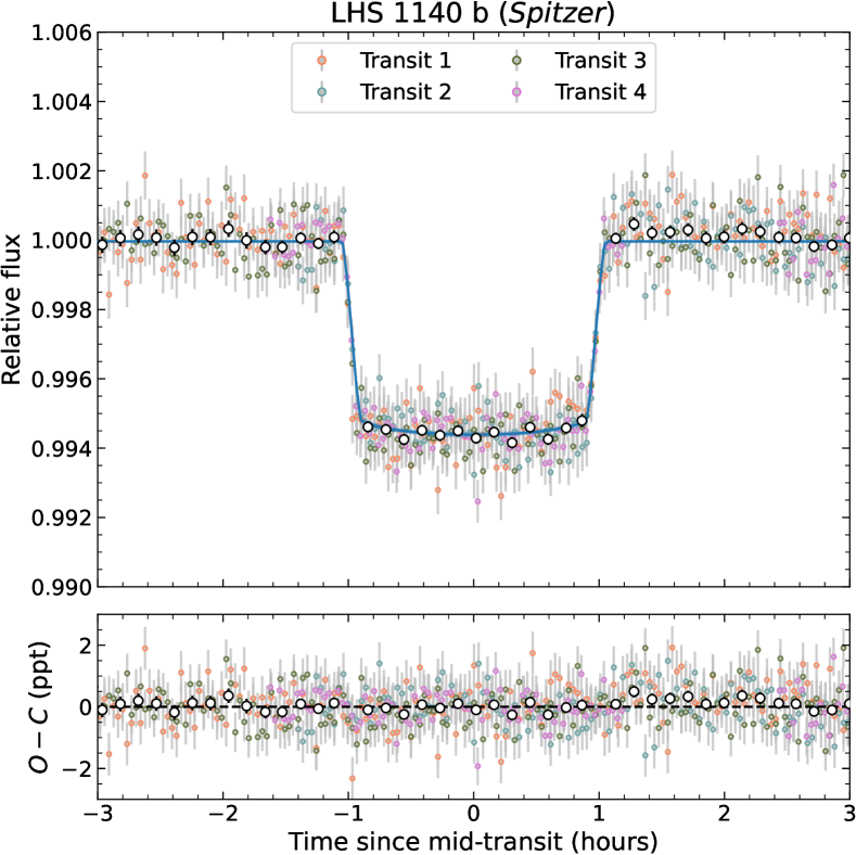
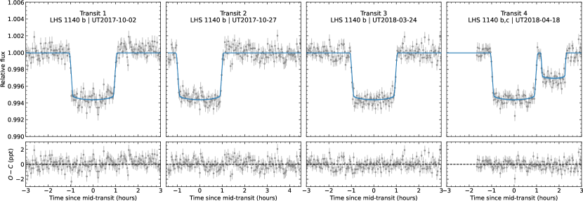
We recovered four Spitzer transits of LHS 1140 b taken with the Infrared Array Camera (Fazio et al., 2004) at 4.5 m from the NASA/IPAC Infrared Science Archive111irsa.ipac.caltech.edu/. These data include the double transit of LHS 1140 b and c analysed by M19, with three additional unpublished transits of LHS 1140 b (PI: J. A. Dittmann) from the same program. The observations were taken on UT2017-10-02, 2017-10-27, 2018-03-24, and 2018-04-18, hereafter referred to as Transit 1 to 4 (Transit 4 is presented in M19).
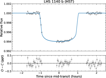
The observations were acquired using the subarray mode with a 2 s exposure producing datacubes of 64 subarray images of 3232 pixels. We used the Spitzer Phase Curve Analysis (SPCA) pipeline (Dang et al., 2018; Bell et al., 2021) to extract the photometry and decorrelate against instrumental systematics. For Transits 1 and 3, we use a 33 pixel area to extract the target’s intensity for each subarray frame. We then median-binned each datacube to mitigate the known subarray instrumental systematics and use Pixel Level Decorrelation (PLD; Deming et al., 2015) to detrend against detector systematics. Similarly to M19, we elect to discard the first 78 minutes of Transit 4 during which the target’s centroid had not yet settled on the detector. For Transit 2 and 4, we opted for a different detrending strategy as the shorter baseline before transit tends to bias the retrieved eclipse depth with PLD. Instead, we find that extracting the target photometry with an exact circular aperture with a radius of 3.0 pixels centered on the target’s centroid yields the optimal photometric scheme. We then binned each datacube and detrended the instrumental systematics using a 2D polynomial as a function of centroid. The stacked (phase-folded) transit of LHS 1140 b is presented in Figure 1. The individual detrended transits are presented Figure A1.
2.2 HST WFC3 white light curve
Two transits of LHS 1140 b were observed with HST WFC3 on UT2017-01-28 and UT2017-12-15 (PN: 14888; PI: J. A. Dittmann). Unfortunately, due to large shifts in the position of the spectrum on the detector, the observation from UT2017-01-28 could not be reliably analysed (Edwards et al., 2021). The transit on UT2017-12-15 was successfully analysed by Edwards et al. (2021) to constrain the transmission spectrum of LHS 1140 b near 1.4 m. The observations were conducted in the G141 grism configuration with the GRISM256 aperture (256256 subarray) and 103.13 s integration time. Readers are referred to Edwards et al. (2021) for a complete description of the HST data reduction that made use of the Iraclis software (Tsiaras et al., 2016). Here, we include the extracted white light curve from HST (Fig. A2) for our transit analysis.
2.3 TESS photometry
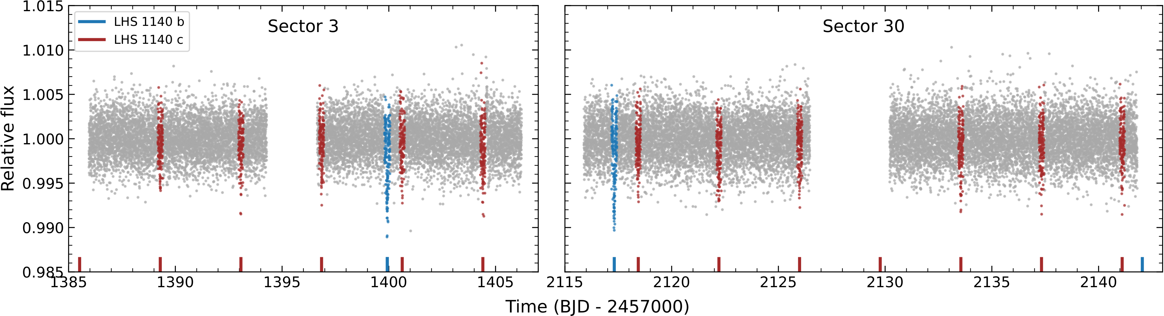
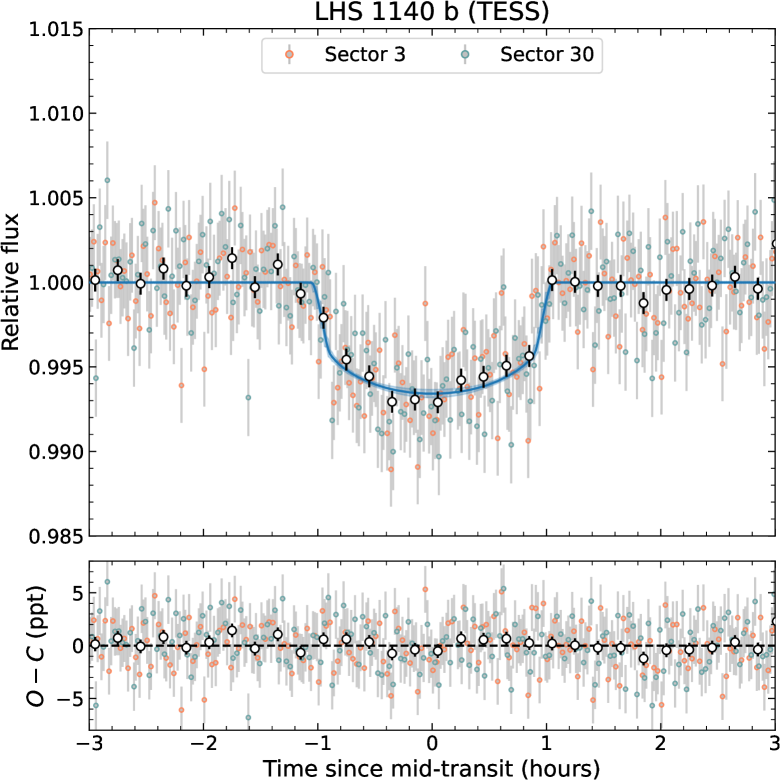
LHS 1140 (TIC 92226327, TOI-256) was observed with TESS at a 2-minute cadence during its primary mission from September 20 to October 17, 2018 (Sector 3) and during its first extended mission from September 23 to October 20, 2020 (Sector 30). We used the Presearch Data Conditioning Simple Aperture Photometry (PDCSAP; Smith et al. 2012; Stumpe et al. 2012, 2014) data product issued by the TESS Science Processing Operations Center (SPOC, Jenkins et al. 2016) at NASA Ames Research Center and available on the Mikulski Archive for Space Telescopes222archive.stsci.edu/tess/. The PDCSAP data includes corrections for instrumental systematics and for flux dilution from known Gaia sources within several TESS pixels (21 per pixel). The light curve from Sector 3 was reprocessed with a more recent release of SPOC (version 5.0.20), which applies the new background correction implemented for the extended mission to the first sectors of TESS. This new correction typically reduces the inferred transit depths by less than 2%. Using the same pipeline (SPOC v5.0) for Sectors 3 and 30 ensures consistent transit depths for LHS 1140 b and c between primary and extended mission data. The full TESS light curve of LHS 1140 shown in Figure A3 captures 2 and 11 transits of planet b and c, respectively, twice as many as in LB20 based on Sector 3 data only. The phase-folded transits from TESS are also shown in the same Figure A3.
2.4 ESPRESSO radial velocity
We retrieved publicly available ESPRESSO data of LHS 1140 from the European Southern Observatory (ESO) science archive333archive.eso.org/ (Delmotte et al., 2006). These data consist of the same 117 spectra analysed in LB20 and taken with the SINGLEHR21 mode between October 2018 and December 2019. We used the bias & dark subtracted, extracted and flat-fielded spectra reduced with the ESPRESSO pipeline (version 2.2.1)444eso.org/sci/software/pipelines/espresso/. The RV extraction from the reduced data was performed with the line-by-line (LBL, version 0.52) method of Artigau et al. (2022) available as an open source package555github.com/njcuk9999/lbl. A simple telluric correction is first performed inside the LBL code by fitting a TAPAS (Bertaux et al., 2014) atmospheric model. This correction step, comparable to the approach of Allart et al. (2022), has been demonstrated to improve the RV precision of ESPRESSO particularly for M-type stars.
At the core of the LBL method, first explored by Dumusque (2018), Doppler shifts are measured on the smallest spectral range possible, i.e., a spectral line, from a high signal-to-noise ratio (SNR) template spectrum of the star and its first derivative (Bouchy et al., 2001). This template is constructed by coadding all our 117 telluric-corrected spectra. Then, the statistical consistency between all per-line velocities (38 000 for LHS 1140) is verified using a simple mixture model (Appendix B of Artigau et al. 2022) that effectively remove high-sigma outliers to produce a final error-weighted average of valid lines. This approach fully exploits the RV content of a stellar spectrum and is conceptually similar to widely employed template-matching algorithms (e.g., Anglada-Escudé & Butler 2012, Astudillo-Defru et al. 2017, Zechmeister et al. 2018, Silva et al. 2022) while being more resilient to outlying spectral features (e.g., telluric residuals, cosmic rays, detector defects).
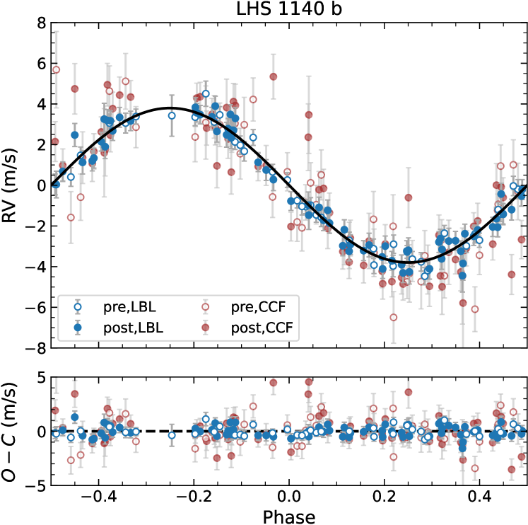
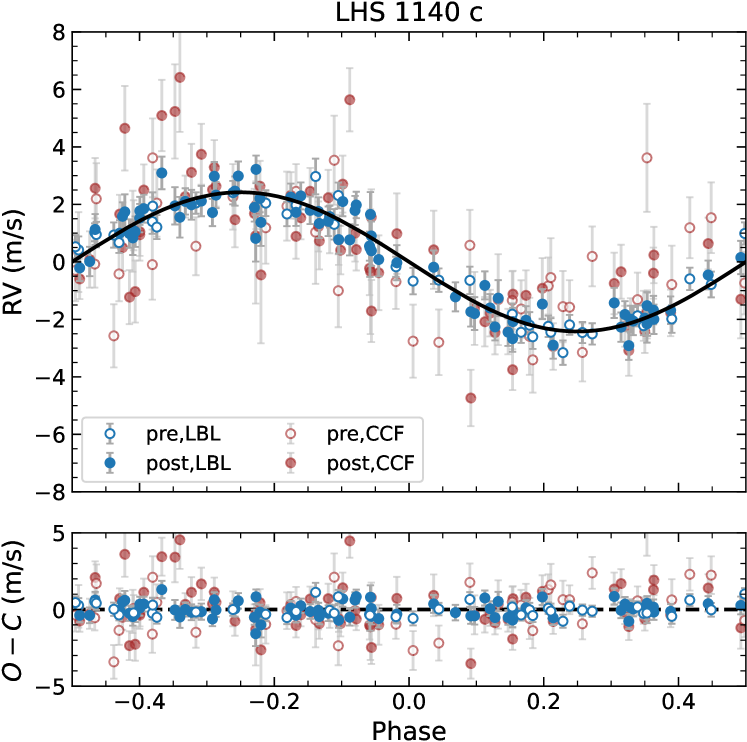
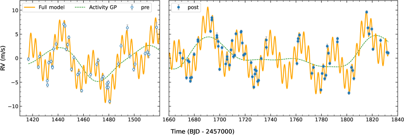
Following LB20, we separately analysed the data taken before and after the fiber link change of ESPRESSO in June 2019 (Pepe et al., 2021), hereafter designated as “pre” and “post” velocities. Using an iterative sigma-clipping algorithm, we removed two epochs (BJD = 2458703.787210 and 2458766.704332) flagged as 3 outliers. The final radial velocities are given in Table B1 and show a median uncertainty of 0.36 m s-1 and dispersion (RMS) of 4.07 m s-1. As a comparison, the published values of LB20 derived from the cross-correlation function (CCF) technique have a median precision of 0.99 m s-1, almost three times larger than LBL, and a 4.76 m s-1 scatter. Figure 2 presents a comparison between LBL and CCF for the best-fit orbits of LHS 1140 b and c. The full LBL RV sequence is shown in Figure B1. Given the extreme precision of ESPRESSO with LBL, a joint analysis with the HARPS data also available through the ESO archive has resulted in identical semi-amplitudes for LHS 1140 b and c. For this reason and to simplify the analysis, we opted to only use ESPRESSO in this work. The ESPRESSO observations span approximately 400 days, a long enough baseline to characterize signals at longer periods, such as the candidate LHS 1140 d ( days) or the rotation of the star ( days; D17). As discussed in Appendices D.1 and D.3, we find no evidence for LHS 1140 d and attribute this 80-day signal most likely to stellar activity.
2.5 NIRPS high-resolution spectroscopy
We acquired 29 high-resolution spectra of LHS 1140 with the Near-InfraRed Planet Searcher (NIRPS; Bouchy et al. 2017; Wildi et al. 2022) during one of its commissioning phases (Prog-ID 60.A-9109) from 2022-11-26 to 2022-12-06. NIRPS is a new echelle spectrograph designed for precision RV at the ESO 3.6-m telescope in La Silla, Chile covering the bands (980–1800 nm). The instrument is equipped with a high-order Adaptive Optics (AO) system and two observing modes, High Accuracy (HA, , 0.4′′ fiber) and High Efficiency (HE, , 0.9′′ fiber), that can both be utilized simultaneously with HARPS. LHS 1140 was observed in HE mode as an RV standard star to test the stability of the instrument preceding the official start of NIRPS operation in April 2023. The observations were reduced with APERO v0.7.271 (Cook et al., 2022), the standard data reduction software for the SPIRou near-infrared spectrograph (Donati et al., 2020), fully compatible with NIRPS. We built a template spectrum of LHS 1140 from the telluric-corrected data product from APERO to derive independent stellar parameters and the abundances of several elements (Sect. 3.2). This template spectrum combines 29 individual spectra each with a SNR per pixel of about 70 in the middle of band.
3 Stellar Characterization
The star LHS 1140 was characterized in previous studies (D17; M19; LB20). In this section, we summarize our work to revise the stellar mass and radius and to measure the effective temperature and stellar abundances with NIRPS. An analysis of the stellar kinematics confirming the age (5 Gyr, D17) and galactic thin disk membership of LHS 1140 is presented in Appendix C.1.
3.1 Stellar mass and radius update
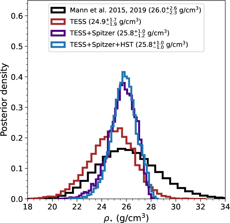
We pulled the magnitude (8.820.02) of LHS 1140 from 2MASS (Skrutskie et al., 2006) and its distance from Gaia DR3 (14.960.01 pc; Gaia Collaboration et al. 2021). Then, from the absolute magnitude () to empirical relation of Mann et al. (2019), we obtain a stellar mass of M⊙, with uncertainty propagating the errors on , , and the scatter of this relation. This revised and more precise stellar mass is consistent with that of M19 ( M⊙) obtained from a similar mass–luminosity calibration (Benedict et al., 2016), but using a smaller sample of nearby binaries. In a similar way, but using the – relationship of Mann et al. (2015), we obtain a radius of R⊙ for LHS 1140. M19 determine the stellar radius from an analysis of the transits, yielding a slightly more precise R⊙. To make sure that our results are completely independent of previous analyses, we first adopt the value derived from Mann et al. (2015) as a prior, then further constrained the radius from the stellar density inferred from transits. This Bayesian method is detailed in Appendix C.2 and results in a new stellar mass and radius of R⊙ and R⊙. The stellar parameters of LHS 1140 are listed in Table C.3.
3.2 Stellar abundances from NIRPS
We follow the methodology of Jahandar et al. (2023), also applied in Cadieux et al. (2022) for TOI-1452 (M4) and in Gan et al. (2023) for TOI-4201 (M0.5), to derive the effective temperature as well as the abundances of several chemical species in LHS 1140 from the NIRPS template spectrum. A global fit ( minimization) to a selection of strong spectral lines using ACES stellar models (Allard et al. 2012; Husser et al. 2013) convolved to match NIRPS resolution resulted in a K and a [M/H] = for LHS 1140. Note we fixed (cgs) for our grid of models in accordance to LHS 1140 (Table C.3). This method was empirically calibrated for log of 5.00.2 dex (Jahandar et al., 2023).
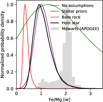
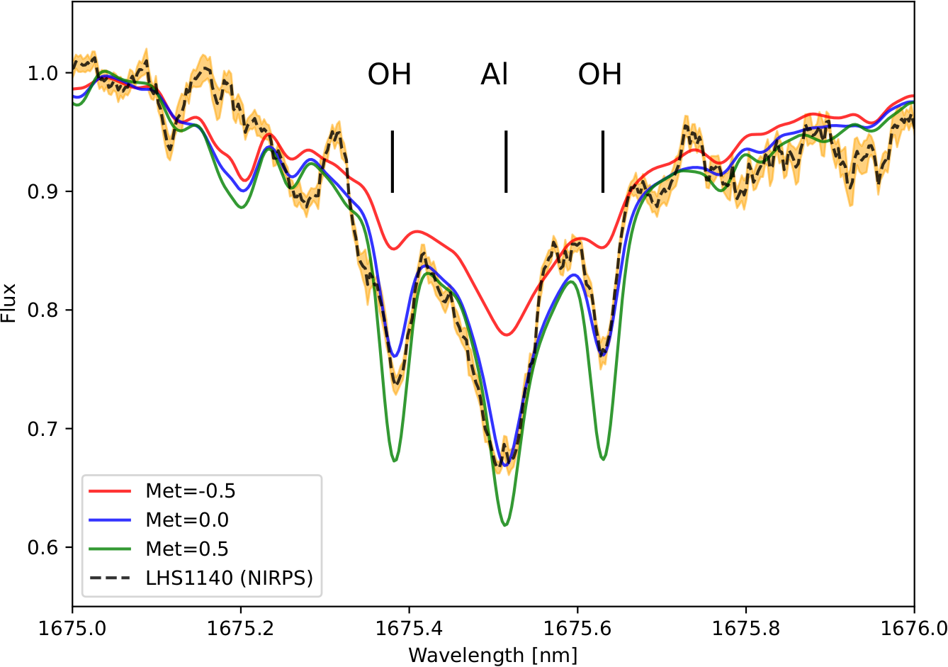
We then performed a series of fits for a fixed K on individual spectral lines of known chemical species to derive their elemental abundances (again following Jahandar et al. 2023). We show an example of this method in Figure C2 for the Al I line at 1675.514 nm from which we measure [Al/H] = dex from this single line. The average abundances for all chemical species detected in LHS 1140 are given in Table C2 including the refractory elements Fe, Mg, and Si that form the bulk material of planetary cores and mantles. As shown in Table C3, LHS 1140 features a relatively low Fe/Mg weight ratio (1.03) compared to the Sun (1.87) and other solar neighbourhood M dwarfs, with a C/O measurement consistent with the solar value. The measured Fe/Mg abundance ratio is used later as input to planetary internal structure models (Sect. 4.2).
4 Results & Discussion
4.1 New density measurements
We measure the physical and orbital parameters of LHS 1140 b and c by jointly fitting transit and Keplerian models to the photometric (Spitzer, HST, and TESS) and RV (ESPRESSO) observations. The details of this joint transit RV fit are presented in Appendix D.1. Notably, the best-fit solution is two planets on circular orbits (Table D1) with no evidence of candidate LHS 1140 d. We adopt the average radius measured by Spitzer and TESS for LHS 1140 c but discuss an important discrepancy between the two measurements in Appendix D.2.
We infer a mass of 5.600.19 M⊕ for LHS 1140 b and 1.910.06 M⊕ for LHS 1140 c, as well as planetary radii of 1.7300.025 R⊕ for b and 1.2720.026 R⊕ for c. The LHS 1140 planets are among the best-characterized exoplanets to date, with relative uncertainties of only 3% for the mass and 2% for the radius, reaching a similar precision to the TRAPPIST-1 planets (Agol et al., 2021). These measurements correspond to bulk densities of g cm-3 and g cm-3 for planet b and c, respectively. The results of previous studies for the semi-amplitudes () and scaled radii () of the planets are shown in Table 1. Since LB20, our updated ratios have increased back to M19 values. This change results from incorporating additional transits with Spitzer and HST, as we retrieve the same as LB20 to 1 when fitting the TESS data only (see Fig. D1). Note our revision of the mass and radius of LHS 1140 b and c is dominated (by more than 80%) by and changes, not by the update of stellar parameters.
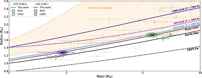
We compare our updated mass and radius to the M dwarf exoplanet population in Figure 3 with various pure composition curves included in the same figure. A detailed analysis of the internal structure of LHS 1140 b is presented in Section 4.2. First examining LHS 1140 b in Figure 3, we see that our revised mass and radius are off the Earth-like track, contradicting previous results from M19 and LB20 that this planet is a rocky, larger version of Earth (super-Earth). The mode of the distribution lies above the pure Mg–Si rock sequence, a region of the mass–radius diagram requiring an additional input of light elements, i.e., gas (H2, He) or ices (e.g., H2O, CH4, NH3), to explain the observed radius. LHS 1140 b is on the lower limit of the synthetic sub-Neptune population around M dwarfs of Rogers et al. 2023 (orange region in Fig. 3) that have undergone thermal evolution and atmospheric mass loss (photoevaporation) over 5 Gyr assuming initial H/He mass fraction between 0.1% and 30%. With a small of 226 K, Rogers et al. 2023 predict a 0.1% H/He mass fraction for LHS 1140 b which we confirm through simulation in Section 4.2.1. Alternatively, the planet could be purely rocky or with a water-mass fraction of 10–20%, clearly not as high as the water-rich (50% H2O) population suggested by Luque & Pallé (2022). Note this latter scenario would involve a different formation mechanism, as suggested by recent studies (Cloutier & Menou, 2020; Luque & Pallé, 2022; Piaulet et al., 2023; Cherubim et al., 2023), where small planets around M dwarfs could directly accrete icy materials outside the water snow line before migrating inwards, in which case sub-Neptunes would actually be water worlds rather than H/He-enveloped planets.
For LHS 1140 c, our mass measurement agrees with previous studies, but we show in Appendix D.2 that Spitzer and TESS radii are in 4 disagreement, complicating the determination of its internal structure. In Figure 3, we present the average Spitzer+TESS radius of LHS 1140 c most compatible with a rocky interior depleted in iron relative to Earth, but should the planet be smaller, as measured by TESS, an Earth-like interior remains plausible. However, given the planet size and higher of 422 K, a hydrogen-dominated atmosphere or an important water content ( by mass) similar to LHS 1140 b are formally rejected.
4.2 Nature of LHS 1140 b
The unprecedented precisions of both the mass and radius of the LHS 1140 planets combined with stellar abundance measurements provide a unique opportunity to better constrain the nature of these planets. Because of the radius uncertainty associated with LHS 1140 c discussed above, we focus our analysis on LHS 1140 b. The mass–radius diagram of Figure 3 suggests three potential scenarios: (1) a mini-Neptune depleted in hydrogen, (2) a pure rocky (and airless) planet and (3) a water world. All three possibilities are discussed below.
To address scenarios 2 and 3, we follow the method of Plotnykov & Valencia (2020) also applied to the water-world candidate TOI-1452 b (Cadieux et al., 2022) to constrain both the core-mass fraction (CMF) and water-mass fraction (WMF) of the planet. The adaptation of this method to LHS 1140 b is further detailed in Appendix E.1 with the posterior distributions available in Appendix E.2. In brief, this interior analysis treats the Fe/Mg ratio either as a free output parameter completely constrained by the mass-radius data (the no prior case) or as direct input informed by the measured stellar value (the stellar prior case) with ). This latter case assumes that stellar abundances are a good proxy of planetary abundances as suggested by planet formation studies (e.g., Bond et al. 2010, Thiabaud et al. 2015, Unterborn et al. 2016) and empirically (e.g., Dorn et al. 2017, Bonsor et al. 2021) though this correlation is not necessarily 1:1 (Adibekyan et al., 2021).
4.2.1 Hydrogen-poor mini-Neptune
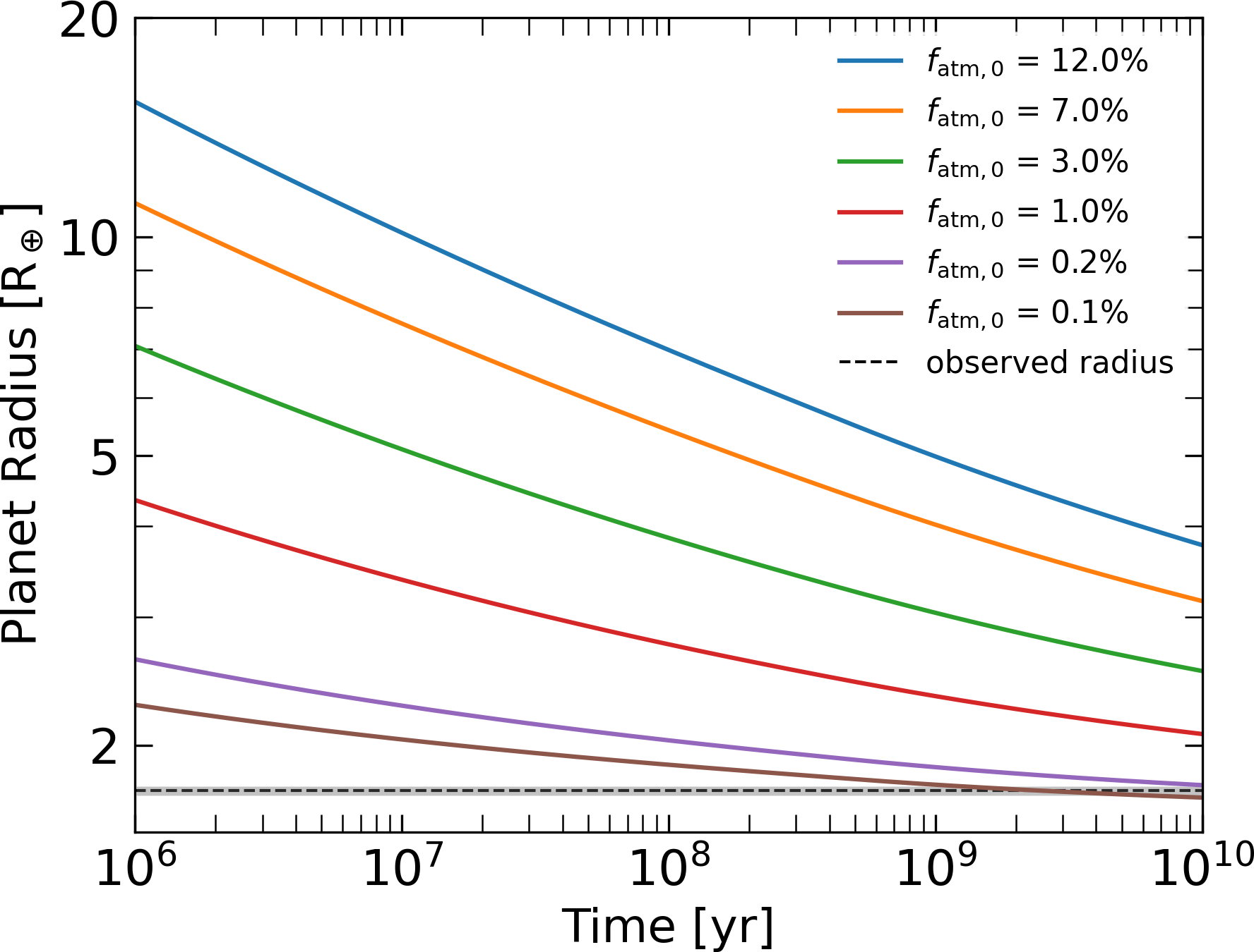
An Earth-like interior (CMF = 33%, WMF 0) overlain by a solar mixture of hydrogen-helium contributing 0.1% of the mass, 10% of the radius could explain the density of LHS 1140 b. Here, we simulate the photoevaporation history of LHS 1140 b for 10 Gyr using the method of Cherubim et al. (2023) to verify whether such hydrogen-rich envelope could survive at present day. These simulations take into account thermal evolution, photoevaporation (e.g., Owen & Wu 2017) from stellar extreme ultraviolet (XUV; 10–130 nm) and core-powered atmospheric escape (e.g., Ginzburg et al. 2018).
The results for a range of initial envelope mass fractions ( between 0.1% and 12%) are shown in Figure 4. Assuming that LHS 1140 b did not undergo important migration after formation, it appears that a –0.2% (brown and purple curves in Fig. 4) is in agreement with the observed radius after 5 Gyr, the minimum age estimate of the system. Since gas accretion models typically predict initial envelopes with mass fractions 1% (Ginzburg et al., 2016), such a small for LHS 1140 b would imply a formation in a gas-poor environment in less than 0.1 Myr (Lee & Connors, 2021) or that it lost part of its atmosphere during giant impacts (Inamdar & Schlichting, 2016). The relatively large semi-major axis of LHS 1140 b (0.1 au) is just beyond the instellation needed to strip the atmosphere: the final after 10 Gyr is close to the initial . In other words, the radius evolution over the simulation timescale is dominated by the cooling/contraction of the atmosphere.
4.2.2 Pure rocky planet
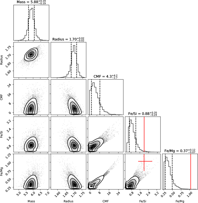
This is the special case of a rocky planet with no water envelope, i.e., the WMF forced to zero. With no prior on the Fe/Mg ratio, our model converges to a very small CMF (%) essentially consistent with a coreless planet with a predicted Fe/Mg ratio (0.37) significantly lower (2.3) than observed for the host star (1.03) and much smaller than the lowest value ever measured in M dwarfs of the solar neighbourhood (see Fig. E1). Moreover, this model converges to a larger mass and smaller radius than observed (2.3 offset in density). We argue that the inconsistency with the observations coupled with the challenge of forming highly iron depleted (coreless) planets (Carter et al. 2015; Scora et al. 2020; Spaargaren et al. 2023) make this scenario implausible for LHS 1140 b. This conclusion is in line with exoplanet demographics (Rogers, 2015) and the empirical rocky-to-gaseous transition around M dwarfs (Cloutier & Menou, 2020) that most 1.6 R⊕ exoplanets are not rocky.
4.2.3 Water world
For this scenario, we also include an atmospheric layer, essentially a (small) fixed radius correction associated with a potential atmosphere. For the general case of a water world receiving more irradiation than the runaway greenhouse threshold ( K; Turbet et al. 2020; Aguichine et al. 2021), the outer layer is likely to be supercritical, which would significantly inflate the radius, requiring a proper joint modeling of the warm water layer in vapor/supercritical state on top of a core+mantle interior. While we defer this general case to a future publication (Plotnykov et al. in prep.), LHS 1140 b with a small K does not warrant such a detailed treatment since a potential outer water layer on this planet is most likely to be either in frozen or liquid state as the planet resides in the Water Condensation Zone (Turbet et al., 2023). We thus assume the atmospheric layer of LHS 1140 b to be an Earth-like atmosphere with a surface pressure of 1 bar and surface temperature equal to . The radius correction (a few tens of kilometers) for such a thin atmosphere is negligible.
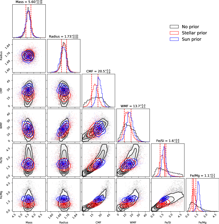
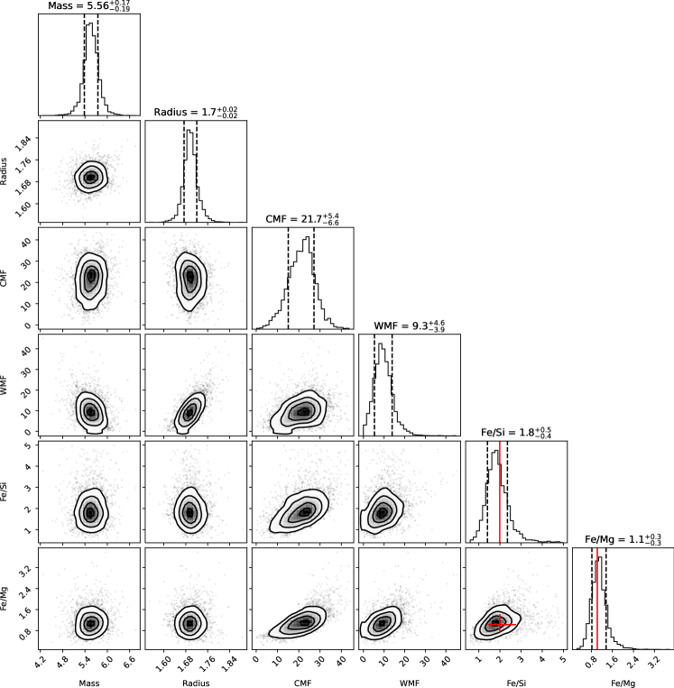
Two prior cases for the Fe/Mg abundance ratio are considered. The unconstrained case (no prior) yields CMF % and a WMF % while assuming that the planet shares the same Fe/Mg ratio as the host star (stellar prior), we obtain CMF % and WMF %. As shown in Table 2, adopting a solar Fe/Mg ratio instead of those measured on LHS 1140 yields an even larger WMF. We tested changing the surface temperature and pressure (using climate predictions from Sect. 4.3) to generate fully solid/liquid water surface. The effect of phase change is small: both CMF and WMF remained within the reported uncertainty for all models.
A variant of this model is the Hycean world (Madhusudhan et al., 2021), i.e., a water world surrounded by a thin H/He-rich layer as was recently proposed for the temperate mini-Neptune K2-18 b (Madhusudhan et al., 2023). This new result opens the possibility that LHS 1140 b may be a lower-mass version of such a Hycean planet in the middle of the radius valley (Fulton et al., 2017). In this scenario, the lower mean molecular weight of the atmosphere yields a higher radius correction (up to 250 km for 2) corresponding to 2% of the planet radius. This case with stellar prior on Fe/Mg still yields a significant WMF % with CMF %.
The main conclusion from this modeling exercise summarized in Table 2 is that LHS 1140 b is unlikely to be a rocky super-Earth. The planet is either a unique mini-Neptune with a thin 0.1% H/He atmosphere or a water world with a WMF in the 9–19% range depending on the atmospheric composition and the Fe/Mg ratio of the planetary interior. Transmission spectroscopic observations with JWST (Gardner et al., 2023) will be key to discriminate between these scenarios.
| Model | CMF (%) | WMF (%) | Fe/Mg [w] |
|---|---|---|---|
| LHS 1140 | |||
| Host star (reference) | – | – | 1.0 |
| LHS 1140 b | |||
| Purely rocky (no prior) | – | ||
| Water world (no prior) | |||
| Water world | |||
| (stellar prior) | |||
| Water world | |||
| (solar prior) | |||
| Hycean world∗ | |||
| (stellar prior) |
Note. — ∗The Hycean model is derived from the Water world model (stellar prior) by subtracting 250 km to the planetary radius corresponding to 5 atmospheric scale heights of H2.
4.3 3D GCM of LHS 1140 b and prospects for atmospheric characterization
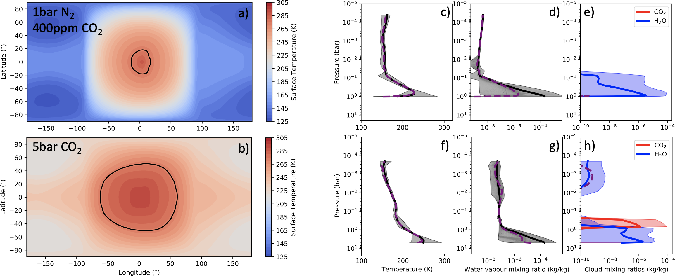
Here we consider the case of a water world with a thin atmosphere for LHS 1140 b as this scenario presents broader implications for habitability. Planets with large amounts of water are likely to have CO2+N2+H2O atmospheres (Forget & Leconte, 2014; Kite & Ford, 2018), possibly with high amounts of CO2 (Marounina & Rogers, 2020). While the diversity of water-world atmospheres has yet to be explored, we adopt here two distinct atmospheric compositions as a first working hypothesis and proof of concept to predict the transmission spectrum of LHS 1140 b: an Earth-like atmosphere (1 bar N2, 400 ppm CO2) and a CO2-dominated atmosphere (5 bar CO2).
The simulations were computed with the Generic Planetary Climate Model (hereafter simply called GCM), a state-of-the-art 3D climate model (Wordsworth et al., 2011) historically known as the LMD (Laboratoire de Météorologie Dynamique, Paris, France) Generic Global Climate Model. The model has been widely applied to simulate all types of exoplanets, ranging from terrestrial planets like the TRAPPIST-1 planets (Turbet et al., 2018; Fauchez et al., 2019) to mini-Neptunes like GJ 1214 b (Charnay et al., 2015) or K2-18 b (Charnay et al., 2021). The GCM uses an up-to-date generalized radiative transfer and can simulate a wide range of atmospheric compositions (N2, H2O, CO2, etc.) including clouds self-consistently.
The model was used to make realistic predictions of LHS 1140 b’s atmospheric properties (temperature–pressure profile, water vapor, and cloud mixing ratios), summarized in Figure 5. We find that no matter how much CO2 is included in the model, the planet has a patch of liquid water at the substellar point. The extent of the ice-free ocean grows with increasing atmospheric CO2, due to the greenhouse effect. This result is similar to that shown by Turbet et al. (2016); Boutle et al. (2017); Del Genio et al. (2018) for Proxima b and Wolf et al. (2017); Turbet et al. (2018); Fauchez et al. (2019) for TRAPPIST-1 planets, that water worlds synchronously rotating in the Habitable Zone of low-mass stars almost always have surface liquid water, at least at the substellar point.
Note that the GCM simulations presented here do not include dynamic ocean and sea ice transport, which could slightly change the extent of the substellar liquid water ocean depending on the amount of CO2 (Del Genio et al., 2019; Yang et al., 2020). Note also that we assumed that LHS 1140 b is in synchronous rotation. This is the most likely rotation mode given LHS 1140 b’s proximity to its star and low eccentricity (Ribas et al., 2016), producing gravitational tides which are expected to dominate atmospheric tides for this planet (Leconte et al., 2015).
The outputs of the GCM were used to compute realistic transmission spectra that take into account the 3D nature of the atmosphere. We used the Planetary Spectrum Generator (PSG; Villanueva et al. 2018, 2022) to produce transmission spectrum models (following the methodology of Fauchez et al. 2019) of LHS 1140 b based on the output of the two GCM simulations including the effects of H2O/CO2 clouds. As shown in Figure 6, the strongest atmospheric feature predicted by these models is CO2 near 4.3 m with a strength of about 15 ppm. Changing the partial pressure of CO2 from 400 ppm to 5 bars produces a similar CO2 bump as this molecule essentially condenses at higher concentration to form ice particles at low altitude (see Fig. 5, panel h).
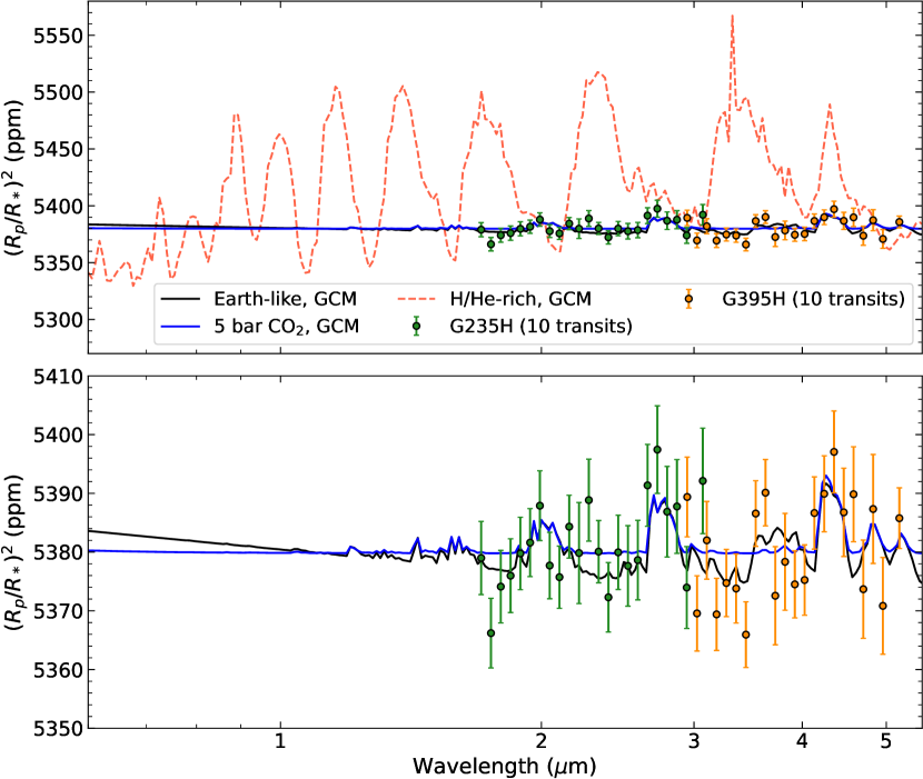
LHS 1140 b was observed twice in transit with JWST in July 2023 during Cycle 1 (PID: 2334, PI: M. Damiano, unpublished). The two visits were made with NIRSpec (Böker et al., 2023) using the Bright Object Time Series mode, one transit with the G235H disperser (1.66–3.05 m) and the other with G395H (2.87–5.14 m). We used PandExo (Batalha et al., 2017) to simulate NIRSpec observations, keeping the same observing strategy of alternating between G235H and G395H. For a degraded spectral resolution of and assuming a conservative 5 ppm noise floor (Coulombe et al., 2023), these simulations predict sensitivity of about 20 ppm for G235H/G395H per spectral bin and per transit. As shown in Figure 6, the Cycle 1 data has the capability to identify the mini-Neptune scenario, but should LHS 1140 b be a water world, we predict that an additional 18 transits (20 in total) would be required to detect its atmosphere (at 4). This estimation is made by simulating 1000 transmission spectra and comparing the log Bayesian evidence () between a flat spectrum and the Earth-like model of Figure 6 with the median simulation shown in the same figure yielding a or 4 (Benneke & Seager, 2013). Note, the optimal observing strategy has yet to be fine-tuned depending on the level of stellar contamination yet to be characterized. This may warrant some visits to be obtained regularly with NIRISS SOSS (0.6–2.8 m; Doyon et al. 2023, Albert et al. 2023).
It should be noted that only four transits are observable every year with JWST as a result of the 24.7-day period of LHS 1140 b and the fact that the system is near the ecliptic. An in-depth atmospheric characterization will realistically require that all future transit events of this planet be observed with JWST over several years (at least 3 years to detect a 15 ppm CO2 signal at 3). Irrespective of the nature of LHS 1140 b, we advocate initiating an extensive campaign as soon as possible considering the uniqueness of this temperate world.
5 Summary & Conclusion
In this letter, we revisited the M4.5 LHS 1140 system hosting two transiting small exoplanets including LHS 1140 b in the Habitable Zone. We applied the novel line-by-line precision radial velocity method of Artigau et al. (2022) to publicly available ESPRESSO data, previously analysed by Lillo-Box et al. (2020) using the cross-correlation function technique. The improvement on the radial velocities is significant: the errors are reduced by almost a factor three, the residual dispersion is halved, and no important excess white noise is detected. By jointly fitting the RVs with transits from Spitzer (3 new archival transits), HST, and TESS (new Sector 30), we update the planetary mass and radius to 5.600.19 M⊕ and 1.7300.025 R⊕ for LHS 1140 b, 1.910.06 M⊕ and 1.2720.026 R⊕ for LHS 1140 c. The improved radial velocity data do not support the existence of the non-transiting candidate LHS 1140 d announced by Lillo-Box et al. (2020).
Our revised mass and radius measurements reveal that LHS 1140 b is unlikely to be a rocky super-Earth as previously reported, as it would require: (1) A density larger (by 2.3) than observed, (2) A core-mass fraction consistent with a coreless planet (CMF %), (3) A planetary Fe/Mg weight ratio smaller (2.3) than measured on its host star and never measured in any solar neighbourhood M dwarfs. Instead, our analysis shows that LHS 1140 b could either be one of the smallest known mini-Neptune (0.1% H/He by mass) with an atmosphere stable to mass loss over the lifetime of the system or a water world with a significant water-mass fraction of % when the iron-to-magnesium weight ratio of the planet is informed by those measured with NIRPS on the host star (Fe/Mg = 1.03). For LHS 1140 c, our updated density is consistent with a rocky world depleted in iron relative to Earth’s, but this result is highly influenced by radius measurement currently discrepant between Spitzer and TESS to 4.
We recommend in-depth transit spectroscopy with JWST to characterize the atmosphere on LHS 1140 b which we predict would create a CO2 feature at 4.3 m, potentially as small as 15 ppm according to self-consistent 3D global climate modeling of the planet in the water world hypothesis. These simulations show that the atmospheric CO2 concentration controls the surface temperature and the extent of a liquid water ocean. For an Earth-like case (1 bar N2, 400 ppm CO2), liquid water is limited to a small patch at the substellar point, while for a CO2-dominated atmosphere (5 bar CO2), almost a whole hemisphere is covered. These future observations could reveal the first exoplanet with a potentially habitable atmosphere and surface.
We thank the anonymous referee for constructive comments and suggestions that improved the presentation of this letter.
This study uses public ESPRESSO data under program IDs 0102.C-0294(A), 0103.C-0219(A), and 0104.C-0316(A) (PI: J. Lillo-Box).
This work is partly supported by the Natural Science and Engineering Research Council of Canada and the Trottier Institute for Research on Exoplanets through the Trottier Family Foundation.
We acknowledge the use of public TESS Alert data from pipelines at the TESS Science Office and at the TESS Science Processing Operations Center. Resources supporting this work were provided by the NASA High-End Computing (HEC) Program through the NASA Advanced Supercomputing (NAS) Division at Ames Research Center for the production of the SPOC data products. This letter includes data collected by the TESS mission that are publicly available from the Mikulski Archive for Space Telescopes (MAST).
This work has been carried out within the framework of the NCCR PlanetS supported by the Swiss National Science Foundation (SNSF) under grants 51NF40_182901 and 51NF40_205606. This project has received funding from the SNSF for project 200021_200726. F.P. would like to acknowledge the SNSF for supporting research with ESPRESSO and NIRPS through grants nr. 140649, 152721, 166227, 184618 and 215190.
This project has received funding from the European Research Council (ERC) under the European Union’s Horizon 2020 research and innovation program (grant agreement SCORE No 851555)
Co-funded by the European Union (ERC, FIERCE, 101052347). Views and opinions expressed are however those of the author(s) only and do not necessarily reflect those of the European Union or the European Research Council. Neither the European Union nor the granting authority can be held responsible for them.
M.T. thanks the Gruber Foundation for its generous support to this research, support from the Tremplin 2022 program of the Faculty of Science and Engineering of Sorbonne University, and the Generic PCM team for the teamwork development and improvement of the model. This work was performed using the High-Performance Computing (HPC) resources of Centre Informatique National de l’Enseignement Supérieur (CINES) under the allocations No. A0100110391 and A0120110391 made by Grand Équipement National de Calcul Intensif (GENCI).
T.J.F. acknowledges support from the GSFC Sellers Exoplanet Environments Collaboration (SEEC), which is funded in part by the NASA Planetary Science Divisions Internal Scientist Funding Model.
R.A. is a Trottier Postdoctoral Fellow and acknowledges support from the Trottier Family Foundation. This work was supported in part through a grant from the Fonds de Recherche du Québec - Nature et Technologies (FRQNT).
J.I.G.H., V.M.P., and A.S.M. acknowledge financial support from the Spanish Ministry of Science and Innovation (MICINN) project PID2020-117493GB-I00 and A.S.M. from the Government of the Canary Islands project ProID2020010129.
This work was supported by Fundação para a Ciência e a Tecnologia (FCT) through national funds and by FEDER through COMPETE2020 - Programa Operacional Competitividade e Internacionalização by these grants: UIDB/04434/2020; UIDP/04434/2020. The research leading to these results has received funding from the European Research Council through the grant agreement 101052347 (FIERCE). E.D.M. acknowledges the support from through Stimulus FCT contract 2021.01294.CEECIND and by the following grants: UIDB/04434/2020 & UIDP/04434/2020 and 2022.04416.PTDC.
B.L.C.M. and J.R.M. acknowledge continuous grants from the Brazilian funding agencies CNPq and Print/CAPES/UFRN. This study was financed in part by the Coordenação de Aperfeiçoamento de Pessoal de Nível Superior - Brasil (CAPES) - Finance Code 001.
T.H. acknowledges support from an NSERC Alexander Graham Bell CGS-D scholarship.
X.D. acknowledges support by the French National Research Agency in the framework of the Investissements d’Avenir program (ANR-15-IDEX-02), through the funding of the “Origin of Life” project of the Grenoble-Alpes University.
References
- Adibekyan et al. (2021) Adibekyan, V., Dorn, C., Sousa, S. G., et al. 2021, Science, 374, 330, doi: 10.1126/science.abg8794
- Agol et al. (2021) Agol, E., Dorn, C., Grimm, S. L., et al. 2021, Planet. Sci. J., 2, 1, doi: 10.3847/PSJ/abd022
- Aguichine et al. (2021) Aguichine, A., Mousis, O., Deleuil, M., & Marcq, E. 2021, ApJ, 914, 84, doi: 10.3847/1538-4357/abfa99
- Ahumada et al. (2020) Ahumada, R., Prieto, C. A., Almeida, A., et al. 2020, ApJS, 249, 3, doi: 10.3847/1538-4365/ab929e
- Akeson et al. (2013) Akeson, R. L., Chen, X., Ciardi, D., et al. 2013, PASP, 125, 989, doi: 10.1086/672273
- Albert et al. (2023) Albert, L., Lafrenière, D., Doyon, R., et al. 2023, Publications of the Astronomical Society of the Pacific, 135, 075001, doi: 10.1088/1538-3873/acd7a3
- Allard et al. (2012) Allard, F., Homeier, D., & Freytag, B. 2012, Philosophical Transactions of the Royal Society of London Series A, 370, 2765, doi: 10.1098/rsta.2011.0269
- Allart et al. (2022) Allart, R., Lovis, C., Faria, J., et al. 2022, A&A, 666, A196, doi: 10.1051/0004-6361/202243629
- Ambikasaran et al. (2015) Ambikasaran, S., Foreman-Mackey, D., Greengard, L., Hogg, D. W., & O’Neil, M. 2015, IEEE Transactions on Pattern Analysis and Machine Intelligence, 38, 252, doi: 10.1109/TPAMI.2015.2448083
- Anglada-Escudé & Butler (2012) Anglada-Escudé, G., & Butler, R. P. 2012, ApJS, 200, 15, doi: 10.1088/0067-0049/200/2/15
- Anglada-Escudé et al. (2016) Anglada-Escudé, G., Amado, P. J., Barnes, J., et al. 2016, Nature, 536, 437, doi: 10.1038/nature19106
- Artigau et al. (2022) Artigau, É., Cadieux, C., Cook, N. J., et al. 2022, AJ, 164, 84, doi: 10.3847/1538-3881/ac7ce6
- Asplund et al. (2021) Asplund, M., Amarsi, A. M., & Grevesse, N. 2021, A&A, 653, A141, doi: 10.1051/0004-6361/202140445
- Astropy Collaboration et al. (2018) Astropy Collaboration, Price-Whelan, A. M., Sipőcz, B. M., et al. 2018, AJ, 156, 123, doi: 10.3847/1538-3881/aabc4f
- Astudillo-Defru et al. (2017) Astudillo-Defru, N., Díaz, R. F., Bonfils, X., et al. 2017, A&A, 605, L11, doi: 10.1051/0004-6361/201731581
- Batalha et al. (2017) Batalha, N. E., Mandell, A., Pontoppidan, K., et al. 2017, PASP, 129, 064501, doi: 10.1088/1538-3873/aa65b0
- Bell et al. (2021) Bell, T. J., Dang, L., Cowan, N. B., et al. 2021, MNRAS, 504, 3316, doi: 10.1093/mnras/stab1027
- Benedict et al. (2016) Benedict, G. F., Henry, T. J., Franz, O. G., et al. 2016, AJ, 152, 141, doi: 10.3847/0004-6256/152/5/141
- Benneke & Seager (2013) Benneke, B., & Seager, S. 2013, ApJ, 778, 153, doi: 10.1088/0004-637X/778/2/153
- Bensby et al. (2003) Bensby, T., Feltzing, S., & Lundström, I. 2003, A&A, 410, 527, doi: 10.1051/0004-6361:20031213
- Bertaux et al. (2014) Bertaux, J. L., Lallement, R., Ferron, S., Boonne, C., & Bodichon, R. 2014, Astronomy & Astrophysics, 564, A46, doi: 10.1051/0004-6361/201322383
- Binney & Tremaine (2008) Binney, J., & Tremaine, S. 2008, Galactic Dynamics: Second Edition
- Blanco-Cuaresma (2019) Blanco-Cuaresma, S. 2019, MNRAS, 486, 2075, doi: 10.1093/mnras/stz549
- Bland-Hawthorn & Gerhard (2016) Bland-Hawthorn, J., & Gerhard, O. 2016, ARA&A, 54, 529, doi: 10.1146/annurev-astro-081915-023441
- Böker et al. (2023) Böker, T., Beck, T. L., Birkmann, S. M., et al. 2023, PASP, 135, 038001, doi: 10.1088/1538-3873/acb846
- Bond et al. (2010) Bond, J. C., O’Brien, D. P., & Lauretta, D. S. 2010, ApJ, 715, 1050, doi: 10.1088/0004-637X/715/2/1050
- Bonsor et al. (2021) Bonsor, A., Jofré, P., Shorttle, O., et al. 2021, MNRAS, 503, 1877, doi: 10.1093/mnras/stab370
- Bouchy et al. (2001) Bouchy, F., Pepe, F., & Queloz, D. 2001, A&A, 374, 733, doi: 10.1051/0004-6361:20010730
- Bouchy et al. (2017) Bouchy, F., Doyon, R., Artigau, É., et al. 2017, The Messenger, 169, 21, doi: 10.18727/0722-6691/5034
- Boutle et al. (2017) Boutle, I. A., Mayne, N. J., Drummond, B., et al. 2017, A&A, 601, A120, doi: 10.1051/0004-6361/201630020
- Cadieux et al. (2022) Cadieux, C., Doyon, R., Plotnykov, M., et al. 2022, AJ, 164, 96, doi: 10.3847/1538-3881/ac7cea
- Carter et al. (2015) Carter, P. J., Leinhardt, Z. M., Elliott, T., Walter, M. J., & Stewart, S. T. 2015, ApJ, 813, 72, doi: 10.1088/0004-637X/813/1/72
- Charnay et al. (2021) Charnay, B., Blain, D., Bézard, B., et al. 2021, A&A, 646, A171, doi: 10.1051/0004-6361/202039525
- Charnay et al. (2015) Charnay, B., Meadows, V., Misra, A., Leconte, J., & Arney, G. 2015, ApJ, 813, L1, doi: 10.1088/2041-8205/813/1/L1
- Cherubim et al. (2023) Cherubim, C., Cloutier, R., Charbonneau, D., et al. 2023, AJ, 165, 167, doi: 10.3847/1538-3881/acbdfd
- Cloutier et al. (2018) Cloutier, R., Doyon, R., Bouchy, F., & Hébrard, G. 2018, AJ, 156, 82, doi: 10.3847/1538-3881/aacea9
- Cloutier & Menou (2020) Cloutier, R., & Menou, K. 2020, AJ, 159, 211, doi: 10.3847/1538-3881/ab8237
- Cook et al. (2022) Cook, N. J., Artigau, É., Doyon, R., et al. 2022, PASP, 134, 114509, doi: 10.1088/1538-3873/ac9e74
- Coulombe et al. (2023) Coulombe, L.-P., Benneke, B., Challener, R., et al. 2023, Nature, 620, 292, doi: 10.1038/s41586-023-06230-1
- Dang et al. (2018) Dang, L., Cowan, N. B., Schwartz, J. C., et al. 2018, Nature Astronomy, 2, 220, doi: 10.1038/s41550-017-0351-6
- Dawson & Johnson (2012) Dawson, R. I., & Johnson, J. A. 2012, ApJ, 756, 122, doi: 10.1088/0004-637X/756/2/122
- Del Genio et al. (2018) Del Genio, A. D., Brain, D., Noack, L., & Schaefer, L. 2018, arXiv e-prints, arXiv:1807.04776. https://arxiv.org/abs/1807.04776
- Del Genio et al. (2019) Del Genio, A. D., Way, M. J., Amundsen, D. S., et al. 2019, Astrobiology, 19, 99, doi: 10.1089/ast.2017.1760
- Delmotte et al. (2006) Delmotte, N., Dolensky, M., Padovani, P., et al. 2006, in Astronomical Society of the Pacific Conference Series, Vol. 351, Astronomical Data Analysis Software and Systems XV, ed. C. Gabriel, C. Arviset, D. Ponz, & S. Enrique, 690
- Deming et al. (2015) Deming, D., Knutson, H., Kammer, J., et al. 2015, ApJ, 805, 132, doi: 10.1088/0004-637X/805/2/132
- Diamond-Lowe et al. (2020) Diamond-Lowe, H., Berta-Thompson, Z., Charbonneau, D., Dittmann, J., & Kempton, E. M. R. 2020, AJ, 160, 27, doi: 10.3847/1538-3881/ab935f
- Dittmann et al. (2017) Dittmann, J. A., Irwin, J. M., Charbonneau, D., et al. 2017, Nature, 544, 333, doi: 10.1038/nature22055
- Donati et al. (2020) Donati, J. F., Kouach, D., Moutou, C., et al. 2020, MNRAS, 498, 5684, doi: 10.1093/mnras/staa2569
- Dorn et al. (2017) Dorn, C., Hinkel, N. R., & Venturini, J. 2017, A&A, 597, A38, doi: 10.1051/0004-6361/201628749
- Doyon et al. (2023) Doyon, R., Willott, C. J., Hutchings, J. B., et al. 2023, PASP, 135, 098001, doi: 10.1088/1538-3873/acd41b
- Dumusque (2018) Dumusque, X. 2018, A&A, 620, A47, doi: 10.1051/0004-6361/201833795
- Edwards et al. (2021) Edwards, B., Changeat, Q., Mori, M., et al. 2021, AJ, 161, 44, doi: 10.3847/1538-3881/abc6a5
- Espinoza (2018) Espinoza, N. 2018, Research Notes of the American Astronomical Society, 2, 209, doi: 10.3847/2515-5172/aaef38
- Espinoza et al. (2019) Espinoza, N., Kossakowski, D., & Brahm, R. 2019, MNRAS, 490, 2262, doi: 10.1093/mnras/stz2688
- Faria et al. (2022) Faria, J. P., Suárez Mascareño, A., Figueira, P., et al. 2022, A&A, 658, A115, doi: 10.1051/0004-6361/202142337
- Fauchez et al. (2019) Fauchez, T. J., Turbet, M., Villanueva, G. L., et al. 2019, ApJ, 887, 194, doi: 10.3847/1538-4357/ab5862
- Fazio et al. (2004) Fazio, G. G., Hora, J. L., Allen, L. E., et al. 2004, ApJS, 154, 10, doi: 10.1086/422843
- Foreman-Mackey (2016) Foreman-Mackey, D. 2016, The Journal of Open Source Software, 1, 24, doi: 10.21105/joss.00024
- Foreman-Mackey et al. (2013) Foreman-Mackey, D., Hogg, D. W., Lang, D., & Goodman, J. 2013, PASP, 125, 306, doi: 10.1086/670067
- Forget & Leconte (2014) Forget, F., & Leconte, J. 2014, Philosophical Transactions of the Royal Society of London Series A, 372, 20130084, doi: 10.1098/rsta.2013.0084
- Fulton et al. (2018) Fulton, B. J., Petigura, E. A., Blunt, S., & Sinukoff, E. 2018, PASP, 130, 044504, doi: 10.1088/1538-3873/aaaaa8
- Fulton et al. (2017) Fulton, B. J., Petigura, E. A., Howard, A. W., et al. 2017, AJ, 154, 109, doi: 10.3847/1538-3881/aa80eb
- Gaia Collaboration et al. (2021) Gaia Collaboration, Brown, A. G. A., Vallenari, A., et al. 2021, A&A, 649, A1, doi: 10.1051/0004-6361/202039657
- Gaia Collaboration et al. (2023) Gaia Collaboration, Vallenari, A., Brown, A. G. A., et al. 2023, A&A, 674, A1, doi: 10.1051/0004-6361/202243940
- Gan et al. (2023) Gan, T., Cadieux, C., Jahandar, F., et al. 2023, AJ, 166, 165, doi: 10.3847/1538-3881/acf56d
- Gardner et al. (2023) Gardner, J. P., Mather, J. C., Abbott, R., et al. 2023, PASP, 135, 068001, doi: 10.1088/1538-3873/acd1b5
- Gillon et al. (2017) Gillon, M., Triaud, A. H. M. J., Demory, B.-O., et al. 2017, Nature, 542, 456, doi: 10.1038/nature21360
- Ginzburg et al. (2016) Ginzburg, S., Schlichting, H. E., & Sari, R. 2016, ApJ, 825, 29, doi: 10.3847/0004-637X/825/1/29
- Ginzburg et al. (2018) —. 2018, MNRAS, 476, 759, doi: 10.1093/mnras/sty290
- Guillot & Morel (1995) Guillot, T., & Morel, P. 1995, A&AS, 109, 109
- Hallatt & Wiegert (2020) Hallatt, T., & Wiegert, P. 2020, AJ, 159, 147, doi: 10.3847/1538-3881/ab7336
- Harris et al. (2020) Harris, C. R., Millman, K. J., van der Walt, S. J., et al. 2020, Nature, 585, 357, doi: 10.1038/s41586-020-2649-2
- Hawkins et al. (2015) Hawkins, K., Jofré, P., Masseron, T., & Gilmore, G. 2015, MNRAS, 453, 758, doi: 10.1093/mnras/stv1586
- Haywood et al. (2014) Haywood, R. D., Collier Cameron, A., Queloz, D., et al. 2014, MNRAS, 443, 2517, doi: 10.1093/mnras/stu1320
- Hemley et al. (1987) Hemley, R. J., Jephcoat, A. P., Mao, H. K., et al. 1987, Nature, 330, 737, doi: 10.1038/330737a0
- Higson et al. (2019) Higson, E., Handley, W., Hobson, M., & Lasenby, A. 2019, Statistics and Computing, 29, 891, doi: 10.1007/s11222-018-9844-0
- Hunter (2007) Hunter, J. D. 2007, Computing in Science and Engineering, 9, 90, doi: 10.1109/MCSE.2007.55
- Husser et al. (2013) Husser, T. O., Wende-von Berg, S., Dreizler, S., et al. 2013, A&A, 553, A6, doi: 10.1051/0004-6361/201219058
- Inamdar & Schlichting (2016) Inamdar, N. K., & Schlichting, H. E. 2016, ApJ, 817, L13, doi: 10.3847/2041-8205/817/2/L13
- Irwin et al. (2009) Irwin, J., Charbonneau, D., Nutzman, P., & Falco, E. 2009, in Transiting Planets, ed. F. Pont, D. Sasselov, & M. J. Holman, Vol. 253, 37–43, doi: 10.1017/S1743921308026215
- Jahandar et al. (2023) Jahandar, F., Doyon, R., Artigau, É., et al. 2023, arXiv e-prints, arXiv:2310.12125, doi: 10.48550/arXiv.2310.12125
- Jenkins et al. (2016) Jenkins, J. M., Twicken, J. D., McCauliff, S., et al. 2016, in Society of Photo-Optical Instrumentation Engineers (SPIE) Conference Series, Vol. 9913, Software and Cyberinfrastructure for Astronomy IV, ed. G. Chiozzi & J. C. Guzman, 99133E, doi: 10.1117/12.2233418
- Karamanis et al. (2021) Karamanis, M., Beutler, F., & Peacock, J. A. 2021, MNRAS, 508, 3589, doi: 10.1093/mnras/stab2867
- Kipping (2010) Kipping, D. M. 2010, MNRAS, 407, 301, doi: 10.1111/j.1365-2966.2010.16894.x
- Kipping (2013) —. 2013, MNRAS, 435, 2152, doi: 10.1093/mnras/stt1435
- Kipping (2014) —. 2014, MNRAS, 440, 2164, doi: 10.1093/mnras/stu318
- Kite & Ford (2018) Kite, E. S., & Ford, E. B. 2018, ApJ, 864, 75, doi: 10.3847/1538-4357/aad6e0
- Kordopatis et al. (2023) Kordopatis, G., Schultheis, M., McMillan, P. J., et al. 2023, A&A, 669, A104, doi: 10.1051/0004-6361/202244283
- Kreidberg (2015) Kreidberg, L. 2015, PASP, 127, 1161, doi: 10.1086/683602
- Leconte et al. (2015) Leconte, J., Wu, H., Menou, K., & Murray, N. 2015, Science, 347, 632, doi: 10.1126/science.1258686
- Lee & Connors (2021) Lee, E. J., & Connors, N. J. 2021, ApJ, 908, 32, doi: 10.3847/1538-4357/abd6c7
- Li & Zhao (2017) Li, C., & Zhao, G. 2017, ApJ, 850, 25, doi: 10.3847/1538-4357/aa93f4
- Lillo-Box et al. (2020) Lillo-Box, J., Figueira, P., Leleu, A., et al. 2020, A&A, 642, A121, doi: 10.1051/0004-6361/202038922
- Lindegren (2018) Lindegren, L. 2018. http://www.rssd.esa.int/doc_fetch.php?id=3757412
- Luque & Pallé (2022) Luque, R., & Pallé, E. 2022, Science, 377, 1211, doi: 10.1126/science.abl7164
- Madhusudhan et al. (2021) Madhusudhan, N., Piette, A. A. A., & Constantinou, S. 2021, ApJ, 918, 1, doi: 10.3847/1538-4357/abfd9c
- Madhusudhan et al. (2023) Madhusudhan, N., Sarkar, S., Constantinou, S., et al. 2023, ApJ, 956, L13, doi: 10.3847/2041-8213/acf577
- Majewski et al. (2016) Majewski, S. R., APOGEE Team, & APOGEE-2 Team. 2016, Astronomische Nachrichten, 337, 863, doi: 10.1002/asna.201612387
- Mann et al. (2015) Mann, A. W., Feiden, G. A., Gaidos, E., Boyajian, T., & von Braun, K. 2015, ApJ, 804, 64, doi: 10.1088/0004-637X/804/1/64
- Mann et al. (2019) Mann, A. W., Dupuy, T., Kraus, A. L., et al. 2019, ApJ, 871, 63, doi: 10.3847/1538-4357/aaf3bc
- Marounina & Rogers (2020) Marounina, N., & Rogers, L. A. 2020, ApJ, 890, 107, doi: 10.3847/1538-4357/ab68e4
- Ment et al. (2019) Ment, K., Dittmann, J. A., Astudillo-Defru, N., et al. 2019, AJ, 157, 32, doi: 10.3847/1538-3881/aaf1b1
- Morrison et al. (2018) Morrison, R. A., Jackson, J. M., Sturhahn, W., Zhang, D., & Greenberg, E. 2018, Journal of Geophysical Research (Solid Earth), 123, 4647, doi: 10.1029/2017JB015343
- Owen & Wu (2017) Owen, J. E., & Wu, Y. 2017, ApJ, 847, 29, doi: 10.3847/1538-4357/aa890a
- Patel & Espinoza (2022) Patel, J. A., & Espinoza, N. 2022, AJ, 163, 228, doi: 10.3847/1538-3881/ac5f55
- Pepe et al. (2002) Pepe, F., Mayor, M., Rupprecht, G., et al. 2002, The Messenger, 110, 9. https://ui.adsabs.harvard.edu/2002Msngr.110....9P/abstract
- Pepe et al. (2021) Pepe, F., Cristiani, S., Rebolo, R., et al. 2021, A&A, 645, A96, doi: 10.1051/0004-6361/202038306
- Piaulet et al. (2023) Piaulet, C., Benneke, B., Almenara, J. M., et al. 2023, Nature Astronomy, 7, 206, doi: 10.1038/s41550-022-01835-4
- Plotnykov & Valencia (2020) Plotnykov, A., & Valencia, D. 2020, MNRAS, 499, 932
- Rajpaul et al. (2015) Rajpaul, V., Aigrain, S., Osborne, M. A., Reece, S., & Roberts, S. 2015, MNRAS, 452, 2269, doi: 10.1093/mnras/stv1428
- Reddy et al. (2006) Reddy, B. E., Lambert, D. L., & Allende Prieto, C. 2006, MNRAS, 367, 1329, doi: 10.1111/j.1365-2966.2006.10148.x
- Reylé et al. (2021) Reylé, C., Jardine, K., Fouqué, P., et al. 2021, A&A, 650, A201, doi: 10.1051/0004-6361/202140985
- Reylé et al. (2022) Reylé, C., Jardine, K., Fouqué, P., et al. 2022, in Cambridge Workshop on Cool Stars, Stellar Systems, and the Sun, Cambridge Workshop on Cool Stars, Stellar Systems, and the Sun, 218, doi: 10.5281/zenodo.7669746
- Ribas et al. (2016) Ribas, I., Bolmont, E., Selsis, F., et al. 2016, A&A, 596, A111, doi: 10.1051/0004-6361/201629576
- Ricker et al. (2015) Ricker, G. R., Winn, J. N., Vanderspek, R., et al. 2015, Journal of Astronomical Telescopes, Instruments, and Systems, 1, 014003, doi: 10.1117/1.JATIS.1.1.014003
- Rogers et al. (2023) Rogers, J. G., Schlichting, H. E., & Owen, J. E. 2023, ApJ, 947, L19, doi: 10.3847/2041-8213/acc86f
- Rogers (2015) Rogers, L. A. 2015, ApJ, 801, 41, doi: 10.1088/0004-637X/801/1/41
- Sabotta et al. (2021) Sabotta, S., Schlecker, M., Chaturvedi, P., et al. 2021, A&A, 653, A114, doi: 10.1051/0004-6361/202140968
- Scora et al. (2020) Scora, J., Valencia, D., Morbidelli, A., & Jacobson, S. 2020, MNRAS, 493, 4910, doi: 10.1093/mnras/staa568
- Seager & Mallén-Ornelas (2003) Seager, S., & Mallén-Ornelas, G. 2003, ApJ, 585, 1038, doi: 10.1086/346105
- Silva et al. (2022) Silva, A. M., Faria, J. P., Santos, N. C., et al. 2022, A&A, 663, A143, doi: 10.1051/0004-6361/202142262
- Skrutskie et al. (2006) Skrutskie, M. F., Cutri, R. M., Stiening, R., et al. 2006, AJ, 131, 1163, doi: 10.1086/498708
- Smith et al. (2012) Smith, J. C., Stumpe, M. C., Van Cleve, J. E., et al. 2012, PASP, 124, 1000, doi: 10.1086/667697
- Spaargaren et al. (2023) Spaargaren, R. J., Wang, H. S., Mojzsis, S. J., Ballmer, M. D., & Tackley, P. J. 2023, ApJ, 948, 53, doi: 10.3847/1538-4357/acac7d
- Speagle (2020) Speagle, J. S. 2020, MNRAS, 493, 3132, doi: 10.1093/mnras/staa278
- Stewart & Ahrens (2005) Stewart, S. T., & Ahrens, T. J. 2005, Journal of Geophysical Research (Planets), 110, E03005, doi: 10.1029/2004JE002305
- Stixrude & Lithgow-Bertelloni (2011) Stixrude, L., & Lithgow-Bertelloni, C. 2011, Geophysical Journal International, 184, 1180, doi: 10.1111/j.1365-246X.2010.04890.x
- Stock et al. (2023) Stock, S., Kemmer, J., Kossakowski, D., et al. 2023, A&A, 674, A108, doi: 10.1051/0004-6361/202244629
- Stumpe et al. (2014) Stumpe, M. C., Smith, J. C., Catanzarite, J. H., et al. 2014, PASP, 126, 100, doi: 10.1086/674989
- Stumpe et al. (2012) Stumpe, M. C., Smith, J. C., Van Cleve, J. E., et al. 2012, PASP, 124, 985, doi: 10.1086/667698
- Suárez Mascareño et al. (2023) Suárez Mascareño, A., González-Álvarez, E., Zapatero Osorio, M. R., et al. 2023, A&A, 670, A5, doi: 10.1051/0004-6361/202244991
- Thiabaud et al. (2015) Thiabaud, A., Marboeuf, U., Alibert, Y., Leya, I., & Mezger, K. 2015, A&A, 580, A30, doi: 10.1051/0004-6361/201525963
- Trotta (2008) Trotta, R. 2008, Contemporary Physics, 49, 71, doi: 10.1080/00107510802066753
- Tsiaras et al. (2016) Tsiaras, A., Waldmann, I. P., Rocchetto, M., et al. 2016, ApJ, 832, 202, doi: 10.3847/0004-637X/832/2/202
- Turbet et al. (2020) Turbet, M., Bolmont, E., Ehrenreich, D., et al. 2020, A&A, 638, A41, doi: 10.1051/0004-6361/201937151
- Turbet et al. (2016) Turbet, M., Leconte, J., Selsis, F., et al. 2016, A&A, 596, A112, doi: 10.1051/0004-6361/201629577
- Turbet et al. (2018) Turbet, M., Bolmont, E., Leconte, J., et al. 2018, A&A, 612, A86, doi: 10.1051/0004-6361/201731620
- Turbet et al. (2023) Turbet, M., Fauchez, T. J., Leconte, J., et al. 2023, arXiv e-prints, arXiv:2308.15110, doi: 10.48550/arXiv.2308.15110
- Unterborn et al. (2016) Unterborn, C. T., Dismukes, E. E., & Panero, W. R. 2016, ApJ, 819, 32, doi: 10.3847/0004-637X/819/1/32
- Valencia et al. (2013) Valencia, D., Guillot, T., Parmentier, V., & Freedman, R. S. 2013, ApJ, 775, 10, doi: 10.1088/0004-637X/775/1/10
- Valencia et al. (2007) Valencia, D., Sasselov, D. D., & O’Connell, R. J. 2007, ApJ, 656, 545, doi: 10.1086/509800
- Van Eylen & Albrecht (2015) Van Eylen, V., & Albrecht, S. 2015, ApJ, 808, 126, doi: 10.1088/0004-637X/808/2/126
- Villanueva et al. (2022) Villanueva, G. L., Liuzzi, G., Faggi, S., et al. 2022, Fundamentals of the Planetary Spectrum Generator
- Villanueva et al. (2018) Villanueva, G. L., Smith, M. D., Protopapa, S., Faggi, S., & Mandell, A. M. 2018, J. Quant. Spec. Radiat. Transf., 217, 86, doi: 10.1016/j.jqsrt.2018.05.023
- Virtanen et al. (2020) Virtanen, P., Gommers, R., Oliphant, T. E., et al. 2020, Nature Methods, 17, 261, doi: 10.1038/s41592-019-0686-2
- Wagner & Pruß (2002) Wagner, W., & Pruß, A. 2002, Journal of Physical and Chemical Reference Data, 31, 387, doi: 10.1063/1.1461829
- Waskom (2021) Waskom, M. 2021, The Journal of Open Source Software, 6, 3021, doi: 10.21105/joss.03021
- Wildi et al. (2022) Wildi, F., Bouchy, F., Doyon, R., et al. 2022, in Society of Photo-Optical Instrumentation Engineers (SPIE) Conference Series, Vol. 12184, Ground-based and Airborne Instrumentation for Astronomy IX, ed. C. J. Evans, J. J. Bryant, & K. Motohara, 121841H, doi: 10.1117/12.2630016
- Wolf et al. (2017) Wolf, E. T., Shields, A. L., Kopparapu, R. K., Haqq-Misra, J., & Toon, O. B. 2017, ApJ, 837, 107, doi: 10.3847/1538-4357/aa5ffc
- Wordsworth et al. (2011) Wordsworth, R. D., Forget, F., Selsis, F., et al. 2011, ApJ, 733, L48, doi: 10.1088/2041-8205/733/2/L48
- Yang et al. (2020) Yang, J., Ji, W., & Zeng, Y. 2020, Nature Astronomy, 4, 58, doi: 10.1038/s41550-019-0883-z
- Zechmeister et al. (2018) Zechmeister, M., Reiners, A., Amado, P. J., et al. 2018, A&A, 609, A12, doi: 10.1051/0004-6361/201731483
Appendix A Light curves
In this appendix, we present the light curves of LHS 1140 from Spitzer, HST, and TESS. The four individual transits of LHS 1140 b and one of LHS 1140 c acquired with Spitzer are presented in Figure A1. The single transit visit from HST with the Wide Field Camera 3 (white light curve) is shown in Figure A2. Lastly, the full TESS light curves from Sectors 3 and 30 are presented in Figure A3.

Appendix B Radial velocity measurements
The ESPRESSO radial velocity of LHS 1140 extracted with the line-by-line method are shown in Figure B1 and listed in Table B1 fully available online.
| BJD - 2 400 000 | RV (m s-1) | (m s-1) |
|---|---|---|
| 58416.711656 | 0.364 | |
| 58424.576752 | 0.360 | |
| 58425.528804 | 0.343 | |
| 58431.527205 | 0.453 | |
| 58431.714392 | 0.423 | |
| 58432.733559 | 0.383 | |
| 58434.555946 | 0.346 | |
| … | … | … |
Note. — Table B1 is published in its entirety in machine-readable format.
Appendix C Supplementary material of the stellar characterization
C.1 Stellar age
We analysed the kinematics of LHS 1140 to characterize its age. This was done by assessing whether the star belongs to the Galaxy’s thin or thick disk stellar populations; thick disk stars are older (10 Gyr) than their counterparts in the thin disk, have different chemistry ([Fe/H]-0.5, [/Fe]+0.3; Reddy et al. 2006), and are kinematically hotter, with larger velocity dispersions relative to the Local Standard of Rest (LSR), and larger orbital excursions from the Galactic midplane (Binney & Tremaine, 2008). We employed the astrometric solution from Gaia DR3 (Gaia Collaboration et al., 2023). We note that the solution’s renormalized unit weight error ruwe=1.53 indicates that there is some uncertainty in the astrometry (ruwe1.4 for well-behaved solutions; Lindegren, 2018). The orbit of LHS 1140 was integrated forward in time 60 Myr using the Monte Carlo model outlined in Hallatt & Wiegert (2020).
These calculations produce a velocity with respect to the Local Standard of Rest km s-1, yielding km s-1 (adopting the Local Standard of Rest from Bland-Hawthorn & Gerhard 2016). This places LHS 1140 in the thin disk, where km s-1 (e.g., Bensby et al., 2003; Hawkins et al., 2015). Its orbital oscillation amplitude above/below the Galactic midplane is pc, significantly smaller than that of thick disk stars (1 kpc; e.g., Li & Zhao 2017) and consistent with that of thin disk stars a few Gyr old (see Fig. 20 of Kordopatis et al., 2023). This result for the age of LHS 1140 is consistent with D17 (5 Gyr) estimated from its slow rotation period and absence of H emission. We thus adopt that LHS 1140 has a relatively old age 5 Gyr and is a thin disk star.
C.2 Bayesian inference of stellar mass and radius from transits
Measured directly from transit light curves, the orbital period () and the scaled semi-major axis () of an exoplanet allow the determination of the density of its host star (Seager & Mallén-Ornelas, 2003):
| (C1) |
While Equation C1 is fundamentally true for all orbits, as it is essentially a reformulation of Kepler’s Third Law (with the gravitational constant), the inferred from transit can be significantly biased when assuming a circular orbit (e.g., Kipping 2010, Dawson & Johnson 2012, Kipping 2014). Following the notation of Van Eylen & Albrecht (2015), the true stellar density () when photo-eccentric effects are considered is given by:
| (C2) |
where and are respectively the orbital eccentricity and argument of periastron of the transiting planet. Unaccounted eccentricity as small as can potentially induce a 30% error in . From our joint transit RV analysis (Appendix D.1), we measure of for LHS 1140 b and for LHS 1140 c consistent with perfectly circular orbits (, with 95% confidence). As both orbital solutions satisfy , we hereafter drop the transit subscript when referring to stellar density obtained from our transit light curves. As summarized in Figure C1, our measurement of constrained by Spitzer, HST, and TESS has resulted in new posteriors for the mass and radius of the star LHS 1140, namely M⊙ and R⊙. This Bayesian approach is taken to improve the precision on and , otherwise the dominant sources of uncertainty for the inferred planetary mass and radius.

C.3 Additional Tables and Figure
We recapitulate the stellar parameters of LHS 1140 in Table C.3. After, we present the stellar abundance determination from NIRPS (Sect. 3.2) in Table C2 and give corresponding chemical weight ratios in Table C3. An example of this chemical spectroscopy analysis for the Al I line (1675.514 nm) is presented in Figure C2.
| Parameter | Value | Ref. |
|---|---|---|
| Astrometry and kinematics | ||
| RA (J2016.0) | 00:44:59.33 | 1 |
| DEC (J2016.0) | -15:16:17.54 | 1 |
| (mas yr-1) | 318.152 0.049 | 1 |
| (mas yr-1) | -596.623 0.054 | 1 |
| (mas) | 66.8287 0.0479 | 1 |
| (pc) | 14.9636 0.0107 | 1 |
| (km s-1) | 14.38 0.041 | 2 |
| (km s-1) | -38.52 0.09 | 2 |
| (km s-1) | 11.18 0.41 | 2 |
| Physical parameters | ||
| (M⊙) | 0.1844 0.0045 | 2 |
| (R⊙) | 0.2159 0.0030 | 2 |
| (g cm-3) | 25.8 1.0 | 3 |
| (K) | 3096 48 | 2 |
| (L⊙) | 0.0038 0.0003 | 3 |
| SpT | M4.5V | 4 |
| (dex) | 0.09 | 2 |
| log (cgs) | 5.041 0.016 | 3 |
| Age | Gyr | 4 |
| (days) | 131 5 | 4 |
| Element | [X/H] | # of lines | |
|---|---|---|---|
| Fe I | -0.15 | 0.09 | 3 |
| Al I | 0.00 | 0.10 | 2 |
| Mg I | 0.11 | 0.10 | 2 |
| Si I | -0.20 | 0.10 | 1 |
| Ca I | 0.20 | 0.10 | 1 |
| O I∗ | 0.00 | 0.01 | 82 |
| C I | 0.10 | 0.10 | 3 |
| 0.01 | 0.04 | – |
Note. — ∗The oxygen abundance is inferred from OH lines.
†Average abundance of all elements.
| Ratios | LHS 1140 | Sun† | M dwarf‡ |
|---|---|---|---|
| Fe/Mg [w] | 1.03 | 1.87 0.22 | [0.89, 2.92] |
| Mg/Si [w] | 1.94 | 0.95 0.09 | [0.69, 1.66] |
| Fe/O [w] | 0.15 | 0.21 0.03 | [0.08, 0.28] |
| C/O [w] | 0.56 | 0.44 0.06 | [0.21, 0.60] |
Note. — ∗Weight ratios calculated using with the absolute logarithmic abundance, taken from Table 2 of Asplund et al. (2021), and the atomic mass of element X.
†Solar weight ratios from Asplund et al. (2021).
‡95% confidence interval of the M dwarf population (1000) of APOGEE DR16 (Majewski et al. 2016; Ahumada et al. 2020)
Appendix D Data analysis
D.1 Joint transit RV fit
The joint analysis of the photometric (Spitzer, HST, and TESS) and RV (ESPRESSO) data is done with juliet (Espinoza, 2018), an all-in-one package that combines transit and RV modeling using batman (Kreidberg, 2015) and radvel (Fulton et al., 2018) with multiple sampling options (e.g., Markov Chain Monte Carlo, nested sampling). Here, we select the dynesty (Speagle, 2020) sampler in juliet for parameter estimations and Bayesian log-evidence () calculations relevant for model comparisons. The dynesty package implements dynamic nested sampling algorithms (Higson et al., 2019) designed for more efficient and robust estimations of complex posterior distributions. We follow the dynesty documentation666dynesty.readthedocs.io/en/stable/index.html and choose the random slice sampling option since the number of free parameters exceeds 20.
The orbit of planet (: ‘b’, ‘c’, ‘d’) is described by four parameters, the orbital period , the time of inferior conjunction , the eccentricity , and the argument of periastron , and one systemic parameter, the stellar density , common for all planets. For multi-planetary systems, a single exists, which eliminates the need to fit semi-major axes () for each planet (Equation C1). We define a Gaussian prior on the stellar density of LHS 1140 based on Mann et al. (2015, 2019): g cm-3. For the transiting planets b and c, we follow the Espinoza et al. (2019) transformation of the transit impact parameter and planet-to-star radius ratio into and parameters to only sample physically plausible regions in – space. We model the baseline flux of the Spitzer, HST, and TESS light curves with the parameter described in Espinoza (2018) and include per-instrument extra jitter terms (, , and ).
Synthetic spectra of M dwarfs often show significant discrepancy with the observations (Blanco-Cuaresma, 2019), implying that theoretical limb-darkening (LD) predictions may be unreliable. Patel & Espinoza (2022) have found systematic offsets between empirical quadratic LD coefficients (,) and theoretical predictions in the TESS bandpass of the order , for cool stars similar to LHS 1140. Differing from previous transit analyses (D17; M19; LB20; Edwards et al. 2021), we do not fix or apply Gaussian priors on the LD coefficients, but let them vary freely (uniform priors). The stellar LD effects in the Spitzer, HST, and TESS transits are modeled using per-instrument quadratic and parameters (Kipping, 2013) constructed to only allow physical solutions for values between 0 and 1. Note fixing the LD parameters to those measured by previous studies for the same instrument does not change the median of our posteriors.
For the Keplerian component, a semi-amplitude for each planet is fitted, as well as instrumental RV offsets (, ) and extra white noise terms (, ) for ESPRESSO pre- and post-fiber upgrade. When testing for possible eccentric orbits, we sample uniformly and between -1 and 1. We include in juliet a Gaussian Process (GP) to model stellar activity in the ESPRESSO RVs. Our GP implementation in juliet runs george (Ambikasaran et al., 2015) with a quasi-periodic covariance kernel (Haywood et al. 2014; Rajpaul et al. 2015):
| (D1) |
where is the time interval between data and , is the amplitude of the GP, is the coherence timescale, scales the periodic component of the GP, and is the stellar rotation period. We adopt a Gaussian prior on the known rotation period of the star days. The priors for the other GP hyperparameters are listed in Table D2 and mostly follow the recommendation of Stock et al. 2023 (GP Prior III) when the rotation period is already constrained.
We inspected three different joint models ():
-
•
Two planets, LHS 1140 b and c, on circular orbits (; , )
-
•
Two planets, LHS 1140 b and c, on eccentric orbits ()
-
•
Three planets, LHS 1140 b, c, and the candidate planet d reported by LB20, on circular orbits (; , )
The difference in Bayesian log-evidence () yields the probability that one model describes better the observations over another. The empirical scale of Trotta 2008 (see Table 1 therein) serves to interpret the significance of and to select the “best” model. A constitutes “strong” evidence in favour of the model with the highest . A corresponds to “moderate” evidence, but a means that neither model should be favoured. Multiple runs of each were carried with dynesty to verify the consistency of .
For the two planet models and , we obtain a in favour of the circular orbit solutions (inconclusive). We report from model upper limits on and (95% confidence) of 0.043 and 0.050, respectively, implying that in all likelihood, the orbit of LHS 1140 b and c are de facto circular. For this reason, we select the simpler as the preferred model. We present the relevant planetary parameters derived from the joint transit RV fit for model in Table D1. The priors and posteriors (16th, 50th, and 84th percentiles) of the free parameters of model are reported in Table D2. The best-fit transit models of the Spitzer, HST, and TESS light curves are respectively shown in Figures 1, A2, and A3. The phase-folded RVs with the best-fit orbital solutions of LHS 1140 b and c is shown in Figure 2 with the full RV model (Keplerian + activity GP) presented in Figure B1. This full RV model yields a residual RMS of 41 cm s-1 for the “pre” data consistent with the median RV errors of 42 cm s-1. For the “post” data, the residual dispersion of 54 cm s-1 is larger than the typical RV errors of 34 cm s-1 so that a cm s-1 jitter term is needed to fully describe the scatter.
The reanalysis of the ESPRESSO data with the LBL framework is an opportunity to test the presence of the candidate LHS 1140 d on a 78.9-day orbit reported by LB20. For model , we chose the same priors on , , and as in LB20, namely days, BJD, and m s-1. This fit converges to a small semi-amplitude of m s-1 and an undefined period of days for a planet d. The Bayesian log-evidence does not increase when adding a third planet with between and . We also reject a larger than 2.21 m s-1 at 2, corresponding to the median signal detected in LB20. LHS 1140 could realistically have other planets, but given the precision of our RV measurements, we see no evidence of an additional companion sharing the parameters of candidate LHS 1140 d. In Appendix D.3, we further demonstrate that an 80-day RV signal is most likely of stellar origin.
D.2 Transit depth discrepancy for LHS 1140 c
In LB20, the radius of LHS 1140 b and c measured by TESS was slightly smaller (by 1.5 and 2 respectively) compared with previous results by M19 obtained with Spitzer (see Fig. 3). Here, our joint analysis of Spitzer, HST (for LHS 1140 b only), and TESS data has resulted in a similar discrepancy for planet c, but not for b. In Figure D1, we show the transit impact parameter () and scaled radius () of LHS 1140 b and c derived from fitting each instrument independently. The – posteriors of LHS 1140 b agree well for all available instruments, but we detect a 4 tension for the of LHS 1140 c measured by Spitzer and TESS.
We remain cautious before interpreting the transit depth discrepancy of LHS 1140 c as real because we only have a single visit with Spitzer. It is possible that data reduction systematics affected the depth measurement. Nonetheless, it is worth mentioning that Spitzer Channel 2 at 4.5 m covers a strong CO2 feature. We detect a difference of 500 ppm between the Spitzer and TESS bandpasses, meaning that if excess atmospheric absorption is causing this discrepancy, it would be readily detectable with JWST. This work calls for better radius determination for LHS 1140 c, particularly obtaining the full near-infrared transmission spectrum of this planet with JWST to reveal its true radius that we currently report as an average between Spitzer and TESS (see Joint in Fig. D1) and test whether its atmosphere is CO2-rich.
| Parameter | LHS 1140 b | LHS 1140 c | Description |
|---|---|---|---|
| Orbital parameters | |||
| (days) | 24.73723 0.00002 | 3.777940 0.000002 | Period |
| (BJD - 2 457 000) | 1399.9300 0.0003 | 1389.2939 0.0002 | Time of inferior conjunction |
| (au) | 0.0946 0.0017 | 0.0270 0.0005 | Semi-major axis |
| (∘) | 89.86 0.04 | 89.80 | Inclination |
| (95%) | (95%) | Eccentricity | |
| Transit parameters | |||
| 0.23 | 0.09 | Impact parameter | |
| (ppt) | 5.38 0.06 | 2.90 0.09 | Depth |
| (hours) | 2.15 0.05 | 1.13 0.02 | Duration |
| Physical parameters | |||
| (R⊕) | 1.730 0.025 | 1.272 0.026 | Radius |
| (M⊕) | 5.60 0.19 | 1.91 0.06 | Mass |
| (g cm-3) | 5.9 0.3 | 5.1 0.4 | Bulk density |
| (S⊕) | 0.43 0.03 | 5.3 0.4 | Insolation |
| (K) | 226 4 | 422 7 | Equilibrium temperature |
| Parameter | Prior1 | Posterior | Description |
|---|---|---|---|
| Stellar parameter | |||
| (g cm-3) | 25.8 1.0 | Stellar density | |
| LHS 1140 b | |||
| (days) | 24.73723 0.00002 | Orbital period | |
| (BJD - 2 457 000) | 1399.9300 0.0003 | Time of inferior conjunction | |
| 0.49 0.03 | Parameterization2 for and | ||
| 0.0733 0.0004 | Parameterization2 for and | ||
| (m s-1) | 3.80 0.11 | RV semi-amplitude | |
| LHS 1140 c | |||
| (days) | 3.777940 0.000002 | Orbital period | |
| (BJD - 2 457 000) | 1389.2939 0.0002 | Time of inferior conjunction | |
| 0.39 0.05 | Parameterization2 for and | ||
| 0.0539 0.0008 | Parameterization2 for and | ||
| (m s-1) | 2.42 0.07 | RV semi-amplitude | |
| Photometric parameters | |||
| 0.016 | Limb-darkening parameter3 | ||
| 0.42 | Limb-darkening parameter3 | ||
| (ppm) | 34 23 | Baseline flux | |
| (ppm) | 15 | Extra white noise | |
| 0.28 0.08 | Limb-darkening parameter3 | ||
| 0.12 | Limb-darkening parameter3 | ||
| (ppm) | 22 | Baseline flux | |
| (ppm) | 12 | Extra white noise | |
| 0.33 | Limb-darkening parameter3 | ||
| 0.56 0.27 | Limb-darkening parameter3 | ||
| (ppm) | 9 48 | Baseline flux | |
| (ppm) | 17 | Extra white noise | |
| RV parameters | |||
| (m s-1) | 1.3 1.5 | RV offset4 | |
| (m s-1) | -0.6 1.4 | RV offset4 | |
| (m s-1) | 0.04 | Extra white noise | |
| (m s-1) | 0.36 0.06 | Extra white noise | |
| RV activity GP | |||
| (m s-1) | 2.8 | Amplitude of the GP | |
| (days) | 164 | Timescale of the GP | |
| 3.7 | Periodic scale of the GP | ||
| (days) | 133 3 | Rotation period |
Note. — is the uniform distribution between value and , is the log-uniform (Jeffreys) distribution between value and , is the normal distribution with mean and variance .
2Parameterization of the transit impact parameter () and the planet-to-star radius ratio () outlined in Espinoza (2018).
are related to the quadratic limb-darkening coefficients by the transformations described in Kipping (2013).
4Relative to the median RV (-13 458.5 and -13 450.5 m s-1 for pre- and post-fiber change data).
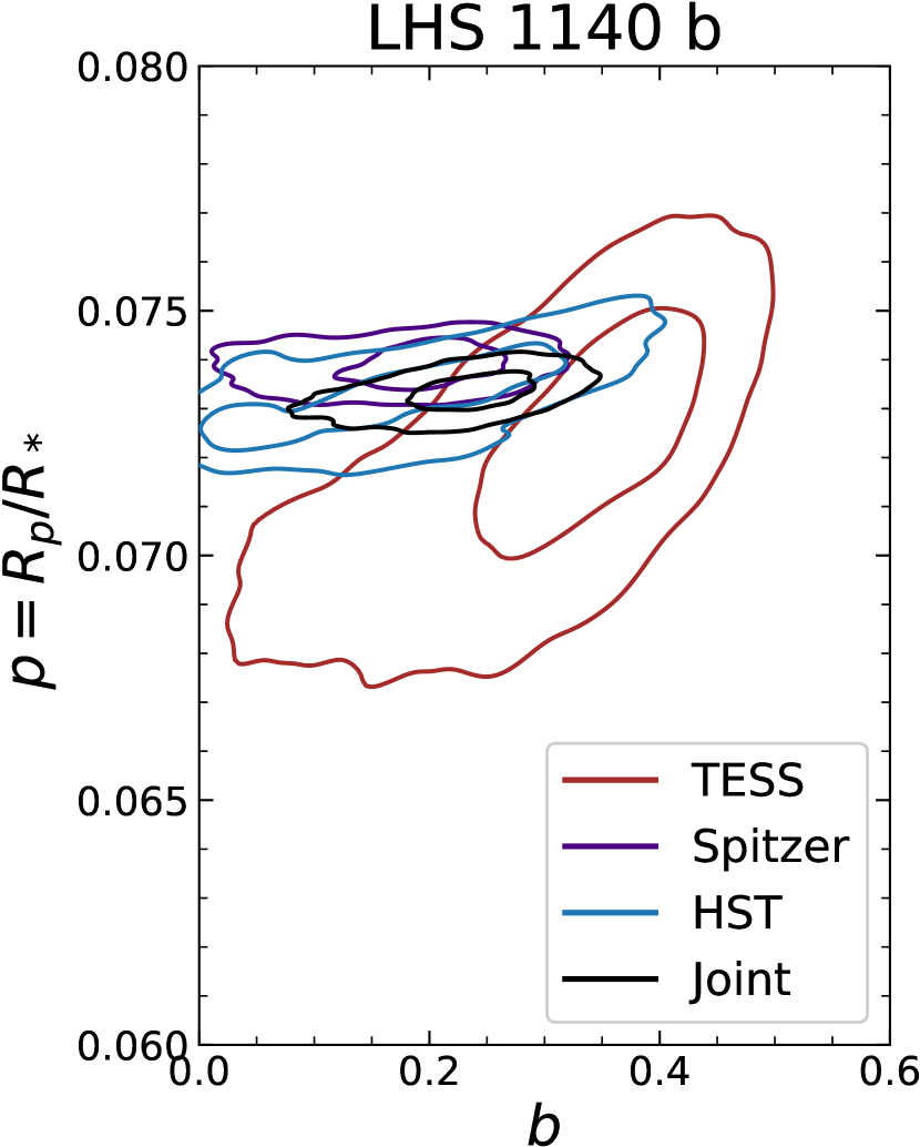
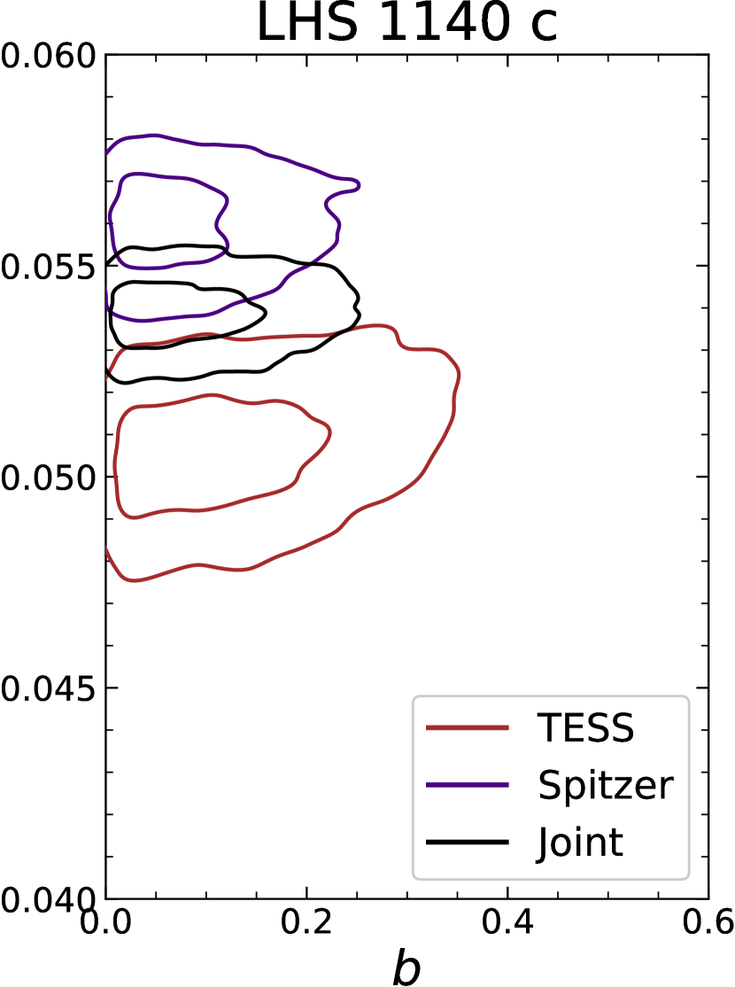
D.3 Validating genuine Keplerian signals with line-by-line radial velocity
The LBL method allows to verify the achromaticity of the inferred semi-amplitudes of the LHS 1140 planets. The three-planet model can be applied on velocities derived per spectral bins of nm in the entire ESPRESSO domain. For genuine Keplerian signals:
-
•
(chromaticity test) the calculated for different bands are achromatic, i.e., .
-
•
(coherence test) the add constructively (coherent period and phase), yielding a consistent weighted average (value and uncertainty) with resulting from the full spectral range.
-
•
(noise test) the semi-amplitude uncertainties () should scale with RV precision () according to the Cloutier et al. (2018) formalism, i.e., when no important extra jitter is detected.
These three criteria can be tested for LHS 1140 b, c, and the non-transiting candidate d. As summarized in Figure D2, we measure no chromaticity for the Keplerian signals of LHS 1140 b and c, respectively with and m s-1 per 100 nm. For the candidate LHS 1140 d, the signal is marginally larger in the blue wavelengths of ESPRESSO ( m s-1 per 100 nm). Similarly, since the Doppler signals of LHS 1140 b and c are perfectly coherent, the weighted average of the are consistent with the obtained from the full spectral range (see Fig. D2). This is not observed for the 80-day signal associated with candidate d for which fitting a Keplerian model on RVs derived from the full ESPRESSO wavelength range is three times less accurate. Finally, given the RV precision of this data set varying from 4.73 to 0.65 m s-1 in the 450–750 nm interval, we find that LHS 1140 b and c follow the Cloutier et al. (2018) formalism, but not d (see Fig. D2, right). Interestingly, the spectral interval 700–725 nm covering only 8% of the ESPRESSO domain contains 30% of all the RV content of LHS 1140. The tests presented in this section provide evidence against the existence of LHS 1140 d first announced by LB20 as a candidate non-transiting planet.
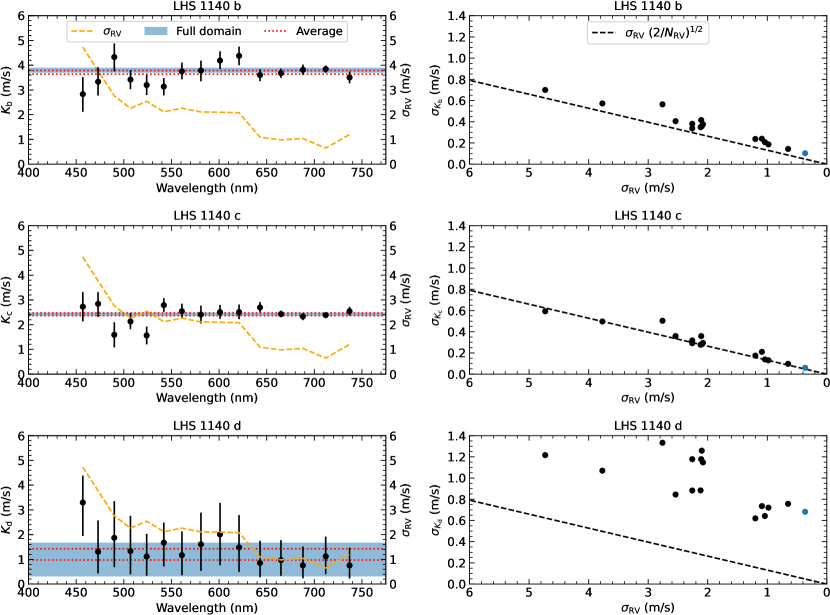
Appendix E Supplementary material of the internal structure analysis
E.1 Interior modeling
In this appendix, we summarize the method of Plotnykov & Valencia (2020) adapted to constrain the detailed internal structure of LHS 1140 b.
We used a Bayesian analysis with Markov Chain Monte Carlo (MCMC) sampling with emcee (Foreman-Mackey et al., 2013) coupled to the internal structure model of Valencia et al. (2007). The model assumes three layers for the interior of the planet: a condensed water (liquid/ice) layer at the surface, a mantle (Mg-Si rock) and a core (Fe-Ni-Si alloy). A fixed atmospheric layer is also considered for models in which the atmosphere could significantly contribute to the planet radius. The water layer is described by the equation of state (EOS) of Hemley et al. 1987; Wagner & Pruß 2002; Stewart & Ahrens 2005 and we adopt the density mixing model with EOS parameters of Stixrude & Lithgow-Bertelloni (2011) and Morrison et al. (2018) for the mantle and the core, respectively. The lower mantle is assumed to be composed of bridgmanite/post-perovskite and wustite (at different proportions to that of Earth), while the upper mantle is modeled as pure olivine (). This choice was made in light of the possible low Si content of the star that may indicate olivine formation is favoured compared to pyroxenes ().
Important ingredients to the model are the abundance ratios (by weight) of refractory elements, namely Fe/Mg and Mg/Si. We explored a no prior (Fe/Mg unconstrained) and a stellar prior (Fe/Mg following the star) models for the water world case of LHS 1140 b (Sect. 4.2.3). For the pure rocky case (Sect. 4.2.2), the planet Fe/Mg ratio must be lower than that of the host star to produce the observed density. Consequently, only the unconstrained Fe/Mg analysis was done. Note that because we model three layers for the interior, the no prior case cannot fully constrain both the CMF and WMF, i.e., planetary interior models are inherently degenerate in this case. For all models, the Mg/Si ratio in the mantle is assumed to be that of the host star: ). Despite LHS 1140 having a Mg/Si approximately twice that of the Sun/Earth (see Table C3), this ratio only weakly influences the final radius of the planet meaning that our results do not depend on the exact mineralogy of the rocks.
E.2 Posterior distributions
We summarize the posterior distributions of Fe/Mg for LHS 1140 b in Figure E1 for the pure rocky (Sect. 4.2.2) and water world (Sect. 4.2.3) scenarios. The posteriors from our MCMC sampling are also presented in the following corner plots of Figures E2, E3, and E4 showing the results for a bare rock, a water world (no prior, stellar prior, and solar prior cases), and a Hycean world, respectively.