Policy Optimization of Finite-Horizon Kalman Filter with Unknown Noise Covariance

Abstract

This paper is on learning the Kalman gain by policy optimization method. Firstly, we reformulate the finite-horizon Kalman filter as a policy optimization problem of the dual system. Secondly, we obtain the global linear convergence of exact gradient descent method in the setting of known parameters. Thirdly, the gradient estimation and stochastic gradient descent method are proposed to solve the policy optimization problem, and further the global linear convergence and sample complexity of stochastic gradient descent are provided for the setting of unknown noise covariance matrices and known model parameters.

Keywords: Kalman filter, linear-quadratic regulator, stochastic gradient descent

1 Introduction

Kalman filter (KF) is widely used in the fields of control and estimation, such as in road vehicle tracking [1, 2, 3], spacecraft orbit estimation and control [4], active power filter [5], medical diagnosis [6], and ship control [7]. However, the noise covariance matrices are usually unknown, and this makes it difficult to use classical KF in practical problems. To solve this puzzle, many approaches have been proposed [8], and there are mainly four types: Bayesian inference, maximum likelihood estimation, innovation correlation and noise variance matching. Bayesian inference uses recursive method to calculate the posterior estimation of unknown parameters under observation, and then calculates the joint posterior probability of state and unknown parameters [9, 10]; maximum likelihood estimation uses nonlinear programming method to calculate the optimal probability density function [11, 12]. Covariance matching technique is to make the covariance of innovation sequence consistent with its theoretical value [13]. Innovation correlation method uses the system output to generate a set of equations related to the model parameters, and solves the these equations to obtain the estimations of unknown parameters; this method has been extensively studied in recent year [14, 15, 16, 17]. Interestingly, most of the analysis of these methods is based on the asymptotic viewpoint.

In this paper, we consider to solve a finite-horizon KF problem (with unknown covariance matrices) from the perspective of policy optimization, namely, to learn the Kalman gain by the stochastic gradient descent (SGD) method. Compared with the aforementioned works, we focus on exploring the global convergence, convergence rate and sample complexity of the SGD method in the policy optimization landscape. The basis of our research is the duality between control and estimation, and the recent developments of policy gradient (PG) method. In the areas of optimal control and reinforcement learning, zeroth-order PG method has been specifically analyzed. The work [18] reformulates the classical linear-quadratic regulator (LQR) as an optimization problem of feedback gain, and obtain the gradient dominance condition and almost smoothness of optimization function by using the advantage function. By the two properties and zeroth-order optimization technique, global linear convergence of gradient descent (GD) method is established in the setting of known parameters and unknown parameters, respectively [18]. Based on this work, the convergence and sample complexity of PG method for several variants of LQR problem are analyzed [19, 20, 21, 22, 23, 24]. For finite-horizon LQR problem, Hambly et al. [19] obtain the global linear convergence of PG method in the setting of both known and unknown parameters, and analyzes the convergence of projected PG method. Mohammadi et al. [21] explore the sample complexity and convergence of PG method for infinite-horizon LQR problem with continuous-time system. Moreover, for LQR problem with risk constraints [22], LQR problem with decentralized system [23], $\mathcal{H}_{2}/\mathcal{H}_{\infty}$ problem [24], the convergence and sample complexity of PG method have also been established.

According to the duality between control and estimation, some convergence results of PG method for solving KF problems have been obtained too [25, 26, 27]. The work [25] develops a receding-horizon policy gradient (RHPG) framework for learning the steady-state Kalman filter, and obtains the sample complexity of convergence of RHPG to optimal filter with error $\epsilon$. In [26], the problem of determining the steady-state Kalman gain is reformulated into a policy optimization problem for the adjoint system, and a SGD method is proposed to learn the steady-state Kalman gain with unknown noise covariance matrices and known model parameters. The work [27] solves the dynamic filter problem for output estimation by policy search method, and proposes a regularizer to establish the global convergence of policy search method.

The objective of this paper is to solve the finite-horizon KF problem with unknown noise covariance matrices. Compared with existing results, our contributions are as follows.

• We introduce a cost function on the observation and prove that the minimizer to this cost function is the Kalman gain; we further construct an unbiased estimation of gradient by using the model parameters and observations, and show the sample complexity and convergence rate of the resulting SGD method. The results of sample complexity indicates that our estimation method needs less samples than that of zeroth-order optimization technique [25], which investigates a steady-state KF problem in the setting of both unknown model parameters and unknown noise covariance matrices.

• The results of this paper can be viewed as an extension of [26] (learning the steady-state KF by a SGD method in the setting of known system parameters and unknown noise covariance matrices) to the setting of handling finite-horizon KF problem, and there are mainly two facts that make our results differ from those of [26]. Firstly, the KF is time-dependent in our setting, and we reformulate the learning problem as an optimal control problem of the dual system, which differs from the deterministic one for the backward adjoint system of [26]. Secondly, we consider the scenario that system noise and observation noise are both subgaussian; though explicit results are just given for the case of Gaussian noise, they can be easily extended to the setting of subgaussian noise by changing some coefficients only. Note that a bounded random variable is subgaussian and the work [26] only considers the scenario of bonded noises. Interestingly, the non-asymptotic error bound of [26] depends explicitly on the bound of the noises.

The rest of this paper is organized as follows. In Section 2, we first review the standard KF, and then introduce some optimization problem which is shown to be equivalent to the finite-horizon KF problem. Section 3 presents the convergence analysis of exact GD algorithm to our optimization problem. In Section 4, we present the form of gradient estimation and the framework of SGD method for solving the finite-horizon KF problem, whose convergence analysis and sample complexity are also studied in this section. Section 5 is a specific discussion on our results and the related works [25, 26]. Section 6 presents some numerical examples to verify the feasibility of the proposed method.

Notation. Let $\mathbb{N}$ be the set of all the natural numbers. For positive integers $n_{0},n_{1},n_{2}$, let $\mathcal{S}^{n_{0}}$ be the set of all the $\mathbb{R}^{n_{0}\times n_{0}}$-valued positive definite matrices, $I_{n_{1}}$ is the $n_{1}\times n_{1}$ unit matrix, $\mathbf{1}_{n_{1}\times n_{1}}$ denotes the $n_{1}\times n_{2}$ matrix whose elements are all $1$, and $0_{n_{1}\times n_{2}}$ is the $n_{1}\times n_{2}$ zero matrix. For a random variable $X$, $\mathbb{E}[X]$ is the mathematical expectation of $X$, $||X||_{L_{2}}$ is the $L_{2}$ norm of $X$, and $||X||_{\psi_{2}}$ is the $\psi_{2}$ norm of $X$. $\sum_{i=k}^{N}a_{i}$ denotes $a_{N}+a_{N-1}+\cdots+a_{k}$ for $k<N$, $a_{k}$ for $k=N$ and $0$ for $k>N$. $\prod_{i=k}^{N}a_{i}$ denotes $a_{N}\times a_{N-1}\times\cdots\times a_{k}$ for $k<N$, $a_{k}$ for $k=N$ and $1$ for $k>N$. For matrix $A$, let $A^{T}$, $||A||$, $||A||_{F}$, $\sigma_{\min}^{A}$ and $\sigma_{\max}^{A}$ be, respectively, the transposition, spectral norm, Frobenius norm, minimal and maximal singular values of $A$, and $A\otimes B$ denotes the kronecker product of matrices $A$ and $B$. If $A$ is square, $tr(A)$ denotes the trace of matrix $A$.

2 Problem formulation

Our goal is to solve a finite-horizon KF problem with unknown noise covariance matrices, which is stated first in this section and then is transformed equivalently into an optimization problem. Without loss of generality, we assume that the initial time $t_{0}$ is $0$ and the terminal time $t_{\max}$ is $M$, and denote $\mathbb{T}=\{0,\dots,M-1\}$.

2.1 Kalman filter

Consider a discrete-time linear time-invariant system

$$\left\{\begin{array}[]{ll}x_{t+1}=Ax_{t}+\omega_{t},\\ y_{t}=Cx_{t}+v_{t},\leavevmode\nobreak\ \leavevmode\nobreak\ \leavevmode\nobreak\ t\in\mathbb{N},\end{array}\right.$$ (1)

where $x_{t}\in\mathbb{R}^{N}$ and $y_{t}\in\mathbb{R}^{m}$ are the state vector and observation vector, respectively, and $x_{0}\sim\mathcal{N}(\overline{x}_{0},\Sigma_{x_{0}})$. In (1), $\{v_{t}\}_{t=0}^{\infty}$ and $\{\omega_{t}\}_{t=0}^{\infty}$ are two sequences of Gaussian random vectors which denote the process noises and measurement noises, respectively, with properties

$$\mathbb{E}[v_{t}]=0,\ \mathbb{E}[\omega_{t}]=0,\ \mathbb{E}[v_{t}v_{t}^{T}]=R_{t},\ \mathbb{E}[\omega_{t}\omega_{t}^{T}]=Q_{t}.$$ (2)

Moreover, $x_{0},v_{t},w_{t},t\in\mathbb{N}$, are assumed to be mutually independent.

As state $x_{t}$ in system (1) cannot be obtained directly in practical problems, the goal of KF is to obtain the optimal estimation $\hat{x}_{t}$ of $x_{t}$ in the mean square sense based on the observation information $\{y_{t}\}$. Specifically, suppose that $\hat{x}_{0}$ has been known and $\hat{x}_{0}=\overline{x}_{0}$, KF can be described as

$$\left\{\begin{array}[]{ll}\widetilde{x}_{t+1}=A\hat{x}_{t},\\ \widetilde{y}_{t+1}=C\widetilde{x}_{t+1},\\ \hat{x}_{t+1}=A\hat{x}_{t}+K_{t}^{*}(y_{t+1}-\widetilde{y}_{t+1}),\leavevmode\nobreak\ \leavevmode\nobreak\ \leavevmode\nobreak\ t\in\mathbb{N},\end{array}\right.$$ (3)

where $\widetilde{x}_{t}$ is the prior estimation of $x_{t}$, and $K_{t}^{*}$ is the Kalman gain to minimize $\mathbb{E}[(x_{t+1}-\hat{x}_{t+1})^{T}(x_{t+1}-\hat{x}_{t+1})]$. In addition, KF can be rewritten as the following form without using prior estimation $\widetilde{x}_{t}$:

$$\left\{\begin{array}[]{l}x_{t+1}=Ax_{t}+\omega_{t},\\ y_{t+1}=Cx_{t+1}+v_{t+1},\\ \hat{x}_{t+1}=A\hat{x}_{t}+K_{t}^{*}CA(x_{t}-\hat{x}_{t})+K_{t}^{*}C\omega_{t}+K_{t}^{*}v_{t+1},\leavevmode\nobreak\ \leavevmode\nobreak\ \leavevmode\nobreak\ t\in\mathbb{N}.\end{array}\right.$$ (4)

Assumption 1.

Let covariance matrices $Q_{t},R_{t},t\in\mathbb{N}$, be positive definite.

The problem we want to solve is to learn Kalman gains $\{K_{t}^{*}\}_{t=0}^{M-1}$ in the setting of unknown noise covariance matrices, which we named the finite-horizon KF problem in what follows. $K_{t}^{*},\ t\in\mathbb{T}$, can be calculated through the following equations

$$P_{t+1}^{*}=AP_{t}^{*}A^{T}+Q_{t}-Z_{t}^{*}(H_{t}^{*})^{-1}Z_{t}^{*T},$$ (5)

$$K_{t}^{*}=Z_{t}^{*}(H_{t}^{*})^{-1}$$ (6)

with

$$H_{t}^{*}=CAP_{t}^{*}(CA)^{T}+R_{t+1}+CQ_{t}C^{T},$$

$$Z_{t}^{*}=AP_{t}^{*}(CA)^{T}+Q_{t}C^{T}.$$

Here, the positive definiteness of $H_{t}^{*}$ is due to Assumption 1. However, $Q_{t},R_{t},t\in\mathbb{T}$, and $P_{0}=\mathbb{E}[(x_{0}-\hat{x}_{0})(x_{0}-\hat{x}_{0})^{T}]$ are unknown in our setting, and solving (5) (6) is not feasible.

2.2 Optimization formulation

In this section, we reformulate the finite-horizon KF problem with unknown noise covariance matrices as an optimization problem, which is stated as the following one.

$\mathbf{Problem\ 1.}$ Find optimal $\mathbf{K}$ such that

$$\min_{\mathbf{K}\in\mathbb{R}^{N\times Mm}}\mathbb{E}\Bigg{[}\sum_{t=0}^{M-1}\sum_{n=1}^{N}(y_{t+n+1}-\hat{y}_{t+1}^{n})^{T}(y_{t+n+1}-\hat{y}_{t+1}^{n})\Bigg{]}$$ (7)

$$\leavevmode\nobreak\ \leavevmode\nobreak\ \leavevmode\nobreak\ \leavevmode\nobreak\ \,\,s.t.\leavevmode\nobreak\ \leavevmode\nobreak\ \leavevmode\nobreak\ \left\{\begin{array}[]{l}x_{t+1}=Ax_{t}+\omega_{t},\\ y_{t+1}=Cx_{t+1}+v_{t+1},\\ \hat{x}_{t+1}=A\hat{x}_{t}+K_{t}CA(x_{t}-\hat{x}_{t})+K_{t}C\omega_{t}+K_{t}v_{t+1},\end{array}\right.$$

where

$$\hat{y}_{t}^{n} :=CA^{n}\hat{x}_{t}=CA^{n}A^{t}\hat{x}_{0}+\sum_{i=0}^{t-1}CA^{n}A^{t-i-1}K_{i}(y_{i+1}-\hat{y}_{i}^{1}),n=1,\dots,N,\ t=1,\dots,M,$$ (8)

$$\mathbf{K} :=(K_{0},\dots,K_{M-1}).$$ (9)

We will use the duality between control and estimation [10, 28] to prove the equivalence between Problem 1 and the finite-horizon KF problem. Note that the optimization function of Problem 1 can be rewritten as

$$tr \Bigg{(}\mathbb{E}\big{[}\sum_{t=0}^{M-1}\sum_{n=1}^{N}(x_{t+1}-\hat{x}_{t+1})(x_{t+1}-\hat{x}_{t+1})^{T}\big{(}CA^{n})^{T}CA^{n}\big{]}\Bigg{)}$$

$$+tr\Bigg{(}\sum_{t=0}^{M-1}\sum_{n=1}^{N}\sum_{i=0}^{n-1}Q_{t+n-i}(CA^{i})^{T}CA^{i}+R_{t+n+1}\Bigg{)};$$

as the second part is a constant, Problem 1 is equal to the following problem.

$\mathbf{Problem\ 2.}$ Find optimal $\mathbf{K}$ such that

$$\min_{\mathbf{K}\in\mathbb{R}^{N\times Mm}}\mathbb{E}\Bigg{[}tr\Bigg{(}\sum_{t=0}^{M-1}{\sum_{n=1}^{N}(x_{t+1}-\hat{x}_{t+1})(x_{t+1}-\hat{x}_{t+1})^{T}(CA^{n})^{T}CA^{n}}\Bigg{)}\Bigg{]}$$ (10)

$$\leavevmode\nobreak\ \leavevmode\nobreak\ \leavevmode\nobreak\ \leavevmode\nobreak\ \,\,\,s.t.\leavevmode\nobreak\ \leavevmode\nobreak\ \leavevmode\nobreak\ \left\{\begin{array}[]{l}x_{t+1}=Ax_{t}+\omega_{t},\\ y_{t+1}=Cx_{t+1}+v_{t+1},\\ \hat{x}_{t+1}=A\hat{x}_{t}+K_{t}CA(x_{t}-\hat{x}_{t})+K_{t}C\omega_{t}+K_{t}v_{t+1}.\end{array}\right.$$

Let us introduce an optimal control problem of the dual system.

$\mathbf{Problem\ 3.}$ Find optimal $\mathbf{K}$ such that

$$\begin{aligned} \leavevmode\nobreak\ \leavevmode\nobreak\ \leavevmode\nobreak\ &\min_{\mathbf{K}\in\mathbb{R}^{m\times MN}}\mathbb{E}\Bigg{[}\sum_{t=0}^{M-1}{\bigg{(}s_{t}^{T}Q_{M-t-1}s_{t}+u_{t}^{T}(CQ_{M-t-1}C^{T}+R_{M-t})u_{t}{+}2u_{t}^{T}CQ_{M-t-1}s_{t}\bigg{)}}+{s_{M}^{T}P_{0}s_{M}}\Bigg{]}\\ &\leavevmode\nobreak\ \leavevmode\nobreak\ \leavevmode\nobreak\ \leavevmode\nobreak\ \leavevmode\nobreak\ \,\,s.t.\leavevmode\nobreak\ \leavevmode\nobreak\ \left\{\begin{array}[]{l}s_{t+1}=A^{T}s_{t}+(CA)^{T}u_{t}+z_{t},\\ u_{t}=-K_{M-t-1}^{T}s_{t},\\ \end{array}\right.\end{aligned}$$ (11)

with

$$s_{0}\sim\mathcal{N}(0,\Sigma),z_{t}\sim\mathcal{N}(0,\Sigma),t=0,\dots,M-2,z_{M-1}=0,$$ (12)

where $s_{0}$ and $z_{t},t\in\mathbb{T}$ are assumed to be mutually independent and $\Sigma=\sum_{n=1}^{N}(CA^{n})^{T}CA^{n}$.

Remark 1.

The dual system of Kalman filter is first introduced in [10], and we here make some changes in the deterministic one of [10] to adapt to system (1) and Problem (10), namely, the dual system in (11) is stochastic. Interestingly, the estimation problem can also be transformed into a LQR problem for some deterministic adjoint system [26], which is a backward equation in time.

The following theorem shows the equivalence between Problem 2 and Problem 3, namely, Problem 2 and Problem 3 can be transformed into a same optimization problem with respect to $\mathbf{K}$. Based on this theorem, the specific proof of equivalence between Problem 1 and the finite-horizon KF problem will be shown in Section 2.3.

To simplify the subsequent proof and for any gains $\mathbf{K}=(K_{0},\dots,K_{M-1})$, let $A_{t}:=A-K_{t}CA,t\in\mathbb{T}$, and denote the optimization function of Problem 2 as

$$f(\mathbf{K}):=\mathbb{E}\Bigg{[}tr\Bigg{(}\sum_{t=0}^{M-1}(x_{t+1}-\hat{x}_{t+1})(x_{t+1}-\hat{x}_{t+1})^{T}\Sigma\Bigg{)}\Bigg{]},$$

where $x_{t},t\in\mathbb{T}$ are generated by $\mathbf{K}$.

Theorem 1.

The optimal solution of Problem 2 is same to the one of Problem 3.

Proof.

The optimization function of Problem 3 can be written as

$$\mathbb{E}\Bigg{[}\bigg{(}\sum_{t=0}^{M-1}s_{t}^{T}Q_{M-t-1}s_{t}+u_{t}^{T}(CQ_{M-t-1}C^{T}+R_{M-t})u_{t}{+}2u_{t}^{T}CQ_{M-t-1}s_{t}\bigg{)}+s_{M}^{T}P_{0}s_{M}\Bigg{]}$$

$$=tr\Bigg{(}\sum_{t=0}^{M-1}\sum_{i=0}^{t}\prod_{j=M-t}^{M-i-1}A_{j}\left((I-K_{M-t-1}C)Q_{M-t-1}(I-K_{M-t-1}C)^{T}+K_{M-t-1}R_{M-t}K_{M-t-1}\right)$$

$$\hphantom{=}\cdot\bigg{(}\prod_{j=M-t}^{M-i-1}A_{j}\bigg{)}^{T}\Sigma\Bigg{)}+tr\left(\sum_{i=0}^{M-1}\prod_{j=0}^{M-i-1}A_{j}P_{0}(\prod_{j=0}^{M-i-1}A_{j})^{T}\Sigma\right).$$ (13)

According to (13), we can rewritten Problem 3 as an optimization problem with respect to $\mathbf{K}$

$$\min_{\mathbf{K}\in\mathbb{R}^{m\times MN}} \Bigg{[}tr\Bigg{(}\sum_{t=0}^{M-1}\sum_{i=0}^{t}\prod_{j=M-t}^{M-i-1}A_{j}((I-K_{M-t-1}C)Q_{M-t-1}(I-K_{M-t-1}C)^{T}$$ (14)

$$+K_{M-t-1}R_{M-t}K_{M-t-1})\bigg{(}\prod_{j=M-t}^{M-i-1}A_{j}\bigg{)}^{T}\Sigma\Bigg{)}+tr\Bigg{(}\sum_{i=0}^{M-1}\prod_{j=0}^{M-i-1}A_{j}P_{0}(\prod_{j=0}^{M-i-1}A_{j})^{T}\Sigma\Bigg{)}\Bigg{]}.$$

Using (2), the optimization function in (14) can be rewritten as

$$tr\Bigg{(}\sum_{t=0}^{M-1}\sum_{i=0}^{M-t-1}\prod_{j=t+1}^{M-i-1}A_{j}((I-K_{t}C)\mathbb{E}[\omega_{t}\omega_{t}^{T}](I-K_{t}C)^{T}+K_{t}\mathbb{E}[v_{t+1}v_{t+1}^{T}]K_{t})(\prod_{j=t+1}^{M-i-1}A_{j})^{T}\Sigma\Bigg{)}$$ (15)

$$+tr\Bigg{(}\sum_{i=0}^{M-1}\prod_{j=0}^{M-i-1}A_{j}\mathbb{E}[(x_{0}-\hat{x}_{0})(x_{0}-\hat{x}_{0})^{T}](\prod_{j=0}^{M-i-1}A_{j})^{T}\Sigma\Bigg{)}.$$

According to (3), we have

$$x_{t+1}-\hat{x}_{t+1}=\sum_{i=0}^{t}\prod_{j=i+1}^{t}A_{j}\big{(}(I-K_{i}C)\omega_{i}-K_{i}v_{i+1}\big{)}+\prod_{j=0}^{t}A_{j}(x_{0}-\hat{x}_{0}),\leavevmode\nobreak\ \leavevmode\nobreak\ t\in\mathbb{T}.$$ (16)

Taking equation (16) into (15), we can obtain the optimization function of Problem 2

$$\mathbb{E}\Bigg{[}tr\Bigg{(}\sum_{t=0}^{M-1}(x_{t+1}-\hat{x}_{t+1})(x_{t+1}-\hat{x}_{t+1})^{T}\Sigma\Bigg{)}\Bigg{]};$$ (17)

this means that Problem 2 can also be transformed into optimization problem (14). This completes the proof. ∎

To simplify the subsequent analysis, we propose the following symbolic

$$\left\{\begin{aligned} &\mathcal{G}_{t}(X):=X+\sum_{i=0}^{M-t-1}\prod_{j=i}^{M-t-1}A_{M-j-1}^{T}XA_{M-j-1},\\ &\mathcal{F}_{t}(X):=A_{M-t-1}^{T}XA_{M-t-1},\\ &\mathcal{D}_{t,s}(X):=\prod_{i=s}^{M-t-1}A_{M-i-1}^{T}XA_{M-i-1},t{,s}\in\mathbb{T},\end{aligned}\right.$$ (18)

where $\mathcal{G}_{t}(X)$ can be rewritten as

$$\mathcal{G}_{t}(X)=X+\sum_{i=0}^{M-t-1}\mathcal{D}_{t,i}(X).$$

2.3 The equivalence between Problem 1 and the finite-horizon KF problem

To prove the equivalence between Problem 1 and the finite-horizon KF problem, we need to calculate $\nabla f(\mathbf{K})$. Let $\mathbf{K}$ be any gain, and define $P_{t}:=\mathbb{E}\big{[}(x_{t}-\hat{x}_{t})(x_{t}-\hat{x}_{t})^{T}\big{]},t=1,\dots,M$, where $\hat{x}_{t},t\in\mathbb{T}$ are the states generated by gains $\mathbf{K}$. Using (10), we obtain

$$P_{t}=A_{t-1}P_{t-1}A_{t-1}^{T}+(I-K_{t-1}C)Q_{t-1}(I-K_{t-1}C)^{T}+K_{t-1}R_{t}K_{t-1}^{T},\leavevmode\nobreak\ \leavevmode\nobreak\ t=1,\dots,M.$$ (19)

Let $H_{t}$ and $Z_{t}$ be

$$H_{t}:=CAP_{t}(CA)^{T}+R_{t+1}+CQ_{t}C^{T},$$

$$Z_{t}:=AP_{t}(CA)^{T}+Q_{t}C^{T},\leavevmode\nobreak\ \leavevmode\nobreak\ \leavevmode\nobreak\ \leavevmode\nobreak\ t\in\mathbb{T}.$$

Theorem 2.

For any $\mathbf{K}\in\mathbb{R}^{m\times MN}$, the gradient $\nabla f(\mathbf{K}):=(\nabla_{0}f(\mathbf{K}),\cdots,\nabla_{M-1}f(\mathbf{K}))$ has the form

$$\nabla_{t}f(\mathbf{K})=2\Sigma_{t}E_{t},\leavevmode\nobreak\ \leavevmode\nobreak\ t\in\mathbb{T},$$ (20)

where $\nabla_{t}f(\mathbf{K})$ is the gradient of $f(\mathbf{K})$ with respect to $K_{t}$ and

$$E_{t} :=\big{(}K_{t}H_{t}-Z_{t}\big{)},$$

$$\Sigma_{t} :=\mathcal{G}_{t+1}(\Sigma).$$

Proof.

We first calculate $\nabla_{0}f(\mathbf{K})$. According to Theorem 1, $f(\mathbf{K})$ is described as

$$f(\mathbf{K})=\mathbb{E}\Bigg{[}\sum_{t=0}^{M-1}s_{t}^{T}Q_{M-t-1}s_{t}+u_{t}^{T}(CQ_{M-t-1}C^{T}+R_{M-t})u_{t}{+}2u_{t}^{T}CQ_{{M-t-1}}s_{t}+s_{M}^{T}P_{0}s_{M}\Bigg{]},$$ (21)

where $s_{t},u_{t},t\in\mathbb{T}$ are defined in Problem 3, and hence $f(\mathbf{K})$ can be transformed into

$$f(\mathbf{K})= \mathbb{E}\Bigg{[}\sum_{t=0}^{M-1}s_{t}^{T}Q_{M-t-1}s_{t}+u_{t}^{T}(CQ_{M-t-1}C^{T}+R_{M-t})u_{t}{+}2u_{t}^{T}CQ_{M-t-1}s_{t}$$

$$+s_{M-1}^{T}A_{0}P_{0}A_{0}^{T}s_{M-1}+z_{M-1}^{T}P_{0}z_{M-1}\Bigg{]}$$

$$= \mathbb{E}\Bigg{[}\sum_{t=0}^{M-2}s_{t}^{T}Q_{M-t-1}s_{t}+u_{t}^{T}(CQ_{M-t-1}C^{T}+R_{M-t})u_{t}{+}2u_{t}^{T}CQ_{M-t-1}s_{t}\Bigg{]}$$

$$+\mathbb{E}\Bigg{[}(s_{M-1}^{T}P_{1}s_{M-1})+z_{M-1}^{T}P_{0}z_{M-1}\Bigg{]}$$ (22)

with $z_{t},t\in\mathbb{T}$ given in Problem 3. Note that the last equality of (22) is by (19). As only $\mathbb{E}\big{[}s_{M-1}^{T}P_{1}s_{M-1}\big{]}$ contains $K_{0}$, $\nabla_{0}f(\mathbf{K})$ is represented as

$$\nabla_{0}f(\mathbf{K})=\nabla_{0}\mathbb{E}\big{[}s_{M-1}^{T}P_{1}s_{M-1}\big{]}=\nabla_{0}tr\big{(}P_{1}\mathbb{E}\big{[}s_{M-1}s_{M-1}^{T}\big{]}\big{)},$$

where

$$\mathbb{E}\big{[}s_{M-1}s_{M-1}^{T}\big{]}= \mathbb{E}\Bigg{[}\Bigg{(}\sum_{t=0}^{M-3}\prod_{i=t+1}^{M-2}A_{M-i-1}^{T}z_{t}+z_{M-2}+\prod_{t=0}^{M-2}A_{M-t-1}^{T}s_{0}\Bigg{)}$$

$$\Bigg{(}\sum_{t=0}^{M-3}\prod_{i=t+1}^{M-2}A_{M-i-1}^{T}z_{t}+z_{M-2}+\prod_{t=0}^{M-2}A_{M-t-1}^{T}s_{0}\Bigg{)}^{T}\Bigg{]}$$

$$= \mathbb{E}\Bigg{[}\sum_{t=0}^{M-3}\mathcal{D}_{1,t+1}(z_{t}z_{t}^{T})+z_{M-2}z_{M-2}^{T}+\mathcal{D}_{1,0}(s_{0}s_{0}^{T})\Bigg{]}$$

$$= \mathcal{G}_{1}(\Sigma)$$

$$= \Sigma_{0}.$$ (23)

As $\Sigma_{0}$ has nothing to do with $K_{0}$, substituting $P_{1}$ into $P_{t}$ of (19) leads to

$$\nabla_{0}f(\mathbf{K})= 2\Sigma_{0}(K_{0}R_{1}-(I-K_{0}C)Q_{0}C^{T}-A_{0}P_{0}(CA)^{T})$$

$$= 2\Sigma_{0}E_{0}.$$

According to (19), $f(\mathbf{K})$ can also be rewritten as

$$f(\mathbf{K})= \mathbb{E}\Bigg{[}\sum_{i=0}^{M-t-1}s_{i}^{T}Q_{M-i-1}s_{i}+u_{i}^{T}(CQ_{M-i-1}C^{T}+R_{M-i})u_{i}{+}2u_{i}^{T}CQ_{M-i-1}s_{i}$$ (24)

$$+s_{M-t}^{T}P_{t}s_{M-t}+\sum_{i=M-t}^{M-1}z_{i}P_{M-i-1}z_{i}\Bigg{]},\leavevmode\nobreak\ \leavevmode\nobreak\ \leavevmode\nobreak\ t=2,\dots,M-1,$$

and

$$f(\mathbf{K})=\mathbb{E}\Bigg{[}s_{0}^{T}P_{M}s_{0}+\sum_{i=0}^{M-1}z_{i}P_{M-i-1}z_{i}\Bigg{]}.$$ (25)

In (24) and (25), only $s_{M-t}^{T}P_{t}s_{M-t}$ contains $K_{t}$ and we have

$$\nabla_{t}f(\mathbf{K})= \nabla_{t}\mathbb{E}[s_{M-t-1}^{T}P_{t+1}s_{M-t-1}]$$

$$= 2\Sigma_{t}E_{t},{\leavevmode\nobreak\ \leavevmode\nobreak\ \leavevmode\nobreak\ t\in\mathbb{T}}.$$

in a similar way. ∎

Using (25), we get the upper bound of $||P_{t}||$

$$||P_{t}||\leq\sum_{i=0}^{M}||P_{i}||\leq\frac{f(\mathbf{K})}{\sigma_{\min}^{\Sigma}}+||P_{0}||,\leavevmode\nobreak\ \leavevmode\nobreak\ t\in\mathbb{T}.$$ (26)

According to the definition of $s_{t},t=0,\dots,M$, we have

$$f(\mathbf{K})= \mathbb{E}\Bigg{[}\sum_{i=0}^{M-t-2}s_{i}^{T}Q_{M-i-1}s_{i}+u_{i}^{T}(CQ_{M-i-1}C^{T}+R_{M-i})u_{i}{\color[rgb]{1,0,0}+}2u_{i}^{T}CQ_{M-i-1}s_{i}$$ (27)

$$+u_{M-t-1}^{T}R_{t+1}u_{M-t-1}+(s_{M-t}-z_{M-t-1})^{T}A^{-T}Q_{t}A^{-1}(s_{M-t}-z_{M-t-1})$$

$$+s_{M-t}^{T}P_{t}s_{M-t}+\sum_{i=M-t}^{M-1}z_{i}P_{M-i-1}z_{i}\Bigg{]}$$

with $t\in\mathbb{T}.$ We obtain the upper bound of $\Sigma_{t},t\in\mathbb{T}$ by (27)

$$||\Sigma_{t}||\leq tr(\Sigma_{t})\leq\frac{f(\mathbf{K})}{\sigma_{\min}^{\mathbf{A^{-T}QA^{-1}}}}+N\sigma_{\max}^{\Sigma},$$ (28)

where $\sigma_{\min}^{\mathbf{A^{-T}QA^{-1}}}$ denotes $\min_{t\in\mathbb{T}}\{\sigma_{\min}^{A^{-T}Q_{t}A^{-1}}\}$. Introduce the notations $\mathcal{A}(\mathbf{K}):=\frac{f(\mathbf{K})}{\sigma_{\min}^{\Sigma}}+||P_{0}||$ and $\mathcal{B}(\mathbf{K}):=\frac{f(\mathbf{K})}{\sigma_{\min}^{\mathbf{A^{-T}QA^{-1}}}}+N\sigma_{\max}^{\Sigma}$ to simplify the subsequent proof.

By Theorem 2 and the following assumption about system (1), we can prove that the optimal solution of Problem 2 satisfies equations (5) and (6); this means the optimal solution of Problem 2 is equal to Kalman gain $\{K_{t}^{*}\}_{t=0}^{M-1}$.

Assumption 2.

The pair $(C,A)$ is observable.

Assumption 3.

Matrix $A$ is invertible.

Corollary 1.

Under assumptions 1-3, the optimal solution of Problem 2 is equal to $\{K_{t}^{*}\}_{t=0}^{M-1}$.

Proof.

Let $\mathbf{K}^{\circ}$ be the optimal solution of Problem 2. Substituting (20) into $\nabla_{t}f(\mathbf{K}^{\circ})=0,\ t\in\mathbb{T}$, we have

$$2\Sigma_{t}(K_{t}H_{t}-Z_{t})=0.$$

Matrix $\Sigma_{t}$ is invertible under Assumption 2 and 3. Therefore, $E_{t}=K_{t}H_{t}-Z_{t}=0$. Due to Assumption 1, we have

$$K_{t}=Z_{t}H_{t}^{-1}.$$ (29)

Taking (29) into (19), $P_{t},\ t\in\mathbb{T}$ satisfy

$$P_{t+1}= A_{t}P_{t}A_{t}^{T}+(I-K_{t}C)Q_{t}(I-K_{t}C)^{T}+K_{t}R_{t+1}K_{t}^{T}$$

$$= AP_{t}A^{T}+Q_{t}-2Z_{t}H_{t}^{-1}Z_{t}+Z_{t}H_{t}^{-1}H_{t}H_{t}^{-1}Z_{t}^{T}$$

$$= AP_{t}A^{T}+Q_{t}-Z_{t}H_{t}^{-1}Z_{t}^{T},$$

which means $P_{t}=P_{t}^{*},t=0,\dots,M$. That completes the proof. ∎

Since Problem 1 is equal to Problem 2, the equivalence between Problem 1 and the finite-horizon KF problem is proved by Corollary 1. For Problem 1, we propose a SGD method in Section 4 to solve it. To analyze the convergence of SGD method, we first analyze the global linear convergence guarantee of exact GD method in Section 3.

2.4 Discussion on Assumption 3

Assumption 3 might be too strong, and it means that the analysis of our method can be applied to the case that the system matrix is invertible. In fact, our initial idea is to solve the following optimization problem instead of Problem 1.

$\mathbf{Problem\ 4.}$ Find optimal $\mathbf{K}$ such that

$$\min_{\mathbf{K}\in\mathbb{R}^{m\times MN}}\mathbb{E}\Bigg{[}tr\Bigg{(}\sum_{t=0}^{M-1}(x_{t+1}-\hat{x}_{t+1})(x_{t+1}-\hat{x}_{t+1})^{T}\Sigma_{initial}\Bigg{)}\Bigg{]}$$ (30)

$$\leavevmode\nobreak\ \leavevmode\nobreak\ \leavevmode\nobreak\ \leavevmode\nobreak\ \,\,\,s.t.\leavevmode\nobreak\ \leavevmode\nobreak\ \leavevmode\nobreak\ \left\{\begin{array}[]{l}x_{t+1}=Ax_{t}+\omega_{t},\\ y_{t+1}=Cx_{t+1}+v_{t+1},\\ \hat{x}_{t+1}=A\hat{x}_{t}+K_{t}CA(x_{t}-\hat{x}_{t})+K_{t}C\omega_{t}+K_{t}v_{t+1},\end{array}\right.$$

where $\Sigma_{initial}=\sum_{n=0}^{N-1}(CA^{n})^{T}CA^{n}$.

Note that there is only a little difference between $\Sigma$ and $\Sigma_{initial}$, and hence the analysis of Problem 2, such as Theorem 2, can be easily extended to the setting for Problem 4. However, it is not easy to rewrite the optimization function of (30) by the observations of system (1) indeed. Specifically, optimization function of Problem 4 is the sum of

$$tr\big{(}\mathbb{E}[(CA^{n}x_{t+1}-CA^{n}\hat{x}_{t+1})(CA^{n}x_{t+1}-CA^{n}\hat{x}_{t+1})^{T}]\big{)},\leavevmode\nobreak\ \leavevmode\nobreak\ t\in\mathbb{T},\leavevmode\nobreak\ \leavevmode\nobreak\ n=0,\dots,N-1.$$ (31)

Using equations (4) and (8), we have

$$\mathbb{E}[(y_{t+n+1}-\hat{y}_{t+1}^{n})^{T}(y_{t+n+1}-\hat{y}_{t+1}^{n})]$$ (32)

$$=tr\big{(}\mathbb{E}[(x_{t+1}-\hat{x}_{t+1})(x_{t+1}-\hat{x}_{t+1})^{T}((CA^{n})^{T}CA^{n})]$$

$$\hphantom{=}-2\mathbb{E}[v_{t+n+1}\hat{x}_{t+1}^{T}]+\mathbb{E}[v_{t+n+1}v_{t+n+1}^{T}]\big{)},\leavevmode\nobreak\ \leavevmode\nobreak\ \leavevmode\nobreak\ t\in\mathbb{T},n=1,\dots,N-1.$$

As $v_{t+n+1}$ is linear independent with $\hat{x}_{t+1}$, we have that $\mathbb{E}[v_{t+n+1}\hat{x}_{t+1}]=0$ and $\mathbb{E}[v_{t+n+1}v_{t+n+1}^{T}]$ is a constant. Therefore, the optimal solution of Problem 4 does not change if we replace $tr\big{(}\mathbb{E}[(CA^{n}x_{t+1}-CA^{n}\hat{x}_{t+1})$ $(CA^{n}x_{t+1}-CA^{n}\hat{x}_{t+1})^{T}]\big{)},t\in\mathbb{T},n=1,\dots,N-1$ by $tr\big{(}\mathbb{E}[(y_{t+n+1}-\hat{y}_{t+n+1}^{n})^{T}(y_{t+n+1}-\hat{y}_{t+1}^{n})]\big{)},t\in\mathbb{T},n=1,\dots,N-1$. On the other hand,

$$\mathbb{E}[(y_{t+1}-\hat{y}_{t+1}^{0})^{T}(y_{t+1}-\hat{y}_{t+1}^{0})]= tr\big{(}\mathbb{E}[(x_{t+1}-\hat{x}_{t+1})(x_{t+1}-\hat{x}_{t+1})^{T}(C^{T}C)]$$ (33)

$$-2\mathbb{E}[\hat{x}_{t+1}v_{t+1}^{T}]+\mathbb{E}[v_{t+1}v_{t+1}^{T}]\big{)},$$

and $\mathbb{E}[\hat{x}_{t+1}v_{t+1}^{T}]=K_{t}R_{t+1}$ is not equal to zero; if we further replace $tr\big{(}\mathbb{E}[(x_{t+1}-\hat{x}_{t+1})(x_{t+1}-\hat{x}_{t+1})^{T}(C^{T}C)]\big{)}$ by $tr\big{(}\mathbb{E}[(y_{t+1}-\hat{y}_{t+1}^{0})^{T}(y_{t+1}-\hat{y}_{t+1}^{0})]\big{)}$, the superfluous term $K_{t}R_{t+1}$ will change the optimal solution of Problem 4, which will be no longer the Kalman gain $\{K_{t}^{*}\}_{t=0}^{M-1}$.

Interestingly, we do not need Assumption 3 in the following special condition. If $R_{t}\equiv R,t\in\mathbb{N}$ and $P_{0}=0$ (i.e., $x_{0}=\hat{x}_{0}$), then we can have the estimation $\hat{R}=\frac{1}{L}\sum_{l=1}^{L}v_{0}(l)v_{0}^{T}(l)$ of covariance matrix $R$ of $v_{t},t\in\mathbb{N}$, by collecting the samples of measurement noise $v_{0}(l)=y_{0}(l)-Cx_{0},l=1,\dots,L$. Therefore, we can replace $tr\big{(}\mathbb{E}[(x_{t+1}-\hat{x}_{t+1})(x_{t+1}-\hat{x}_{t+1})^{T}(C^{T}C)]\big{)}$ in Problem 4 by $tr(\mathbb{E}[(y_{t+1}-\hat{y}_{t+1}^{0})^{T}(y_{t+1}-\hat{y}_{t+1}^{0})]+2K_{t}\hat{R})$ without changing the optimal solution of Problem 4, and hence we can propose a learning method like Algorithm 1 below for Problem 4 and analyze the sample complexity and convergence of the new algorithm as the same as we will do in Section 4.

Indeed, Assumption 3 has been proposed in the classical Mehra method [8], which is used to estimate the noise covariance. The necessity of this condition has yet to be proved [16], and whether the Kalman gain can be obtained in the setting with singular $A$ has been not addressed. In the near future, we might explore how to weaken this assumption in the perspective of optimization.

3 Exact GD method

In this section, we first review some properties of $f(\mathbf{K})$ and analyze the convergence of exact GD method. Though the model of our optimization problem is different from the ones of existing literature, the proofs of this section are essentially same to those of [19] due to the relationship between Kalman filter and Kalman predictor. Just for the completeness, we present some concise proofs of the concerned results.

Suppose that covariance matrices $P_{0}$, $\{Q_{t}\}_{t\in\mathbb{T}},$ $\{R_{t+1}\}_{t\in\mathbb{T}}$ and model parameters $A,C$ are all known, and in this section we will analyze the convergence of exact GD method for Problem 2. To simplify the subsequent proofs, we introduce the following notations. Let $\mathbf{K}^{\prime}=(K_{0}^{\prime},K_{1}^{\prime},\dots,K_{M-1}^{\prime})$ be any gain and $\mathbf{K}^{*}=(K_{0}^{*},K_{1}^{*},\dots,K_{M-1}^{*})$ be the optimal solution of Problem 2, and $A_{t}^{\prime},P_{t+1}^{\prime},\Sigma_{t}^{\prime},E_{t}^{\prime},A_{t}^{*},\Sigma_{t}^{*},E_{t}^{*},t\in\mathbb{T}$ are defined in the same way as $A_{t},P_{t+1},\Sigma_{t},E_{t}$, where we just replace $K_{t}$ by $K_{t}^{\prime}$ and $K_{t}^{*}$, respectively. Let $\{s_{t}^{\prime}\}$ and $\{u_{t}^{\prime}\}$ denote the state sequence and control sequence generated by policy $\mathbf{K}^{\prime}$, and further let $\sigma_{\max}^{\mathbf{CQC^{T}+R}}$, $\sigma_{\min}^{\mathbf{R}}$ denote $\max_{t\in\mathbb{T}}\{\sigma_{\max}^{CQ_{t}C^{T}+R_{t+1}}\}$ and $\min_{t\in\mathbb{T}}\{\sigma_{\min}^{R_{t+1}}\}$, respectively. Denote

$$\Lambda_{t}:=(CQ_{t}C^{T})+R_{t+1}+CAP_{t}(CA)^{T},$$ (34)

$$\delta K_{t}^{\prime}:=K_{t}^{\prime}-K_{t},\leavevmode\nobreak\ \leavevmode\nobreak\ \leavevmode\nobreak\ t\in\mathbb{T},$$

$$||\Lambda_{\max}||:=\sigma_{\max}^{\mathbf{CQC^{T}+R}}+||CA||^{2}\mathcal{A}(\mathbf{K}).$$

The Polyak-Lojasiewicz (PL) condition is key to analyze the convergence of exact GD method, and it can be deduced in several different versions of LQR problem [18, 19, 20, 25, 26]. Lemma 1 and Lemma 2 below are simple extensions of Lemma 3.6 and Lemma 3.7 of [19], which shows that $f(\mathbf{K})$ also has the PL condition and almost smoothness. Note that the expression (21) of $f(\mathbf{K})$ contains a cross term between $u_{t}$ and $s_{t}$; this makes the coefficients $c_{1},c_{2}$ of (35) (36) slightly different from those in [19]. For the completeness, this paper presents a concise proof of Lemma 1, which is same to that of Lemma 3.6 of [19].

Lemma 1.

Under assumptions 1-3 and for any $\mathbf{K}\in\mathbb{R}^{N\times mM}$, $f(\mathbf{K})$ satisfies the following inequalities:

$$f(\mathbf{K})-f(\mathbf{K}^{*}) \leq c_{1}tr\Bigg{(}\sum_{t=0}^{M-1}\nabla_{t}f(\mathbf{K})\nabla_{t}f(\mathbf{K})^{T}\Bigg{)},$$ (35)

$$f(\mathbf{K})-f(\mathbf{K}^{*}) \geq c_{2}tr\Bigg{(}\sum_{t=0}^{M-1}E_{t}E_{t}^{T}\Bigg{)},$$ (36)

where $c_{1}=\frac{\mathcal{B}(\mathbf{K}^{*})}{4\sigma_{\min}^{R}(\sigma_{\min}^{\Sigma})^{2}}$ and $c_{2}=\frac{\sigma_{\min}^{\Sigma}}{4(\sigma_{\max}^{\mathbf{CQC^{T}+R}}+||CA||^{2}\mathcal{A}(\mathbf{K}))}$.

Proof.

The advantage function takes the form

$$A(\mathbf{K}^{\prime},\mathbf{K})= f(\mathbf{K}^{\prime})-f(\mathbf{K})$$

$$= \mathbb{E}\Bigg{[}\sum_{t=0}^{M-1}s_{t}^{\prime T}Q_{M-t-1}s_{t}^{\prime}+u_{t}^{\prime T}(CQ_{M-t-1}C^{T}+R_{M-t})u_{t}^{\prime}{+}2u_{t}^{\prime T}CQ_{M-t-1}s_{t}^{\prime}$$

$$+s_{t+1}^{\prime}P_{M-t-1}s_{t+1}^{\prime}-s_{t}^{\prime}P_{M-t}s_{t}^{\prime}-z_{t}P_{M-t-1}z_{t}^{T}\Bigg{]}$$

$$= tr\Bigg{(}\sum_{t=0}^{M-1}\Sigma_{t}^{\prime}(E_{t}\Lambda_{t}^{-1}+\delta K_{t}^{\prime})\Lambda_{t}(E_{t}\Lambda_{t}^{-1}+\delta K_{t}^{\prime})^{T}-\Sigma_{t}^{\prime}E_{t}\Lambda_{t}^{-1}(E_{t})^{T}\Bigg{)}.$$ (37)

Substituting ${\mathbf{K}^{\prime}=\mathbf{K}^{*}}$ into (37), we obtain

$$A(\mathbf{K}^{*},\mathbf{K}) \geq-tr\Bigg{(}\sum_{t=0}^{M-1}\Sigma_{t}^{*}E_{t}\Lambda_{t}^{-1}(E_{t})^{T}\Bigg{)}.$$ (38)

Dividing both sides of (38) by -1 and using inequalities $||\Lambda_{t}^{-1}||\leq\frac{1}{\sigma_{\min}^{\mathbf{R}}}$, $||\Sigma_{t}^{-1}||\leq\frac{1}{\sigma_{\min}^{\Sigma}}$, we have

$$f(\mathbf{K})-f(\mathbf{K}^{*})\leq\sum_{t=0}^{M-1}\frac{||\Sigma_{t}^{*}||}{4\sigma_{\min}^{\mathbf{R}}(\sigma_{\min}^{\Sigma})^{2}}||\nabla_{t}f(\mathbf{K})||_{F}^{2}.$$

According to (28), $c_{1}=\frac{\mathcal{B}(\mathbf{K}^{*})}{4\sigma_{\min}^{R}(\sigma_{\min}^{\Sigma})^{2}}\geq\frac{||\Sigma_{t}^{*}||}{4\sigma_{\min}^{\mathbf{R}}(\sigma_{\min}^{\Sigma})^{2}}$, and hence we get (35). Similarly, substituting $\hat{K}_{t}=K_{t}-E_{t}\Lambda_{t}^{-1}$ into $K_{t}^{\prime}$ of (37), it holds

$$f(\mathbf{K})-f(\mathbf{K}^{*})\geq f(\mathbf{K})-f(\mathbf{\hat{K}})\geq\sum_{t=0}^{M-1}\frac{\sigma_{\min}^{\Sigma}}{4||\Lambda_{\max}||}||E_{t}||_{F}^{2}\geq\sum_{t=0}^{M-1}c_{2}||E_{t}||_{F}^{2}.$$ (39)

This completes the proof. ∎

Using Lemma 1, $\sum_{t=0}^{M-1}||K_{t}||$ can be bounded in the following way

$$\sum_{t=0}^{M-1}||K_{t}|| \leq\sum_{t=0}^{M-1}\Bigg{(}\frac{||(K_{t}H_{t}-Z_{t})||+||Z_{t}||}{\sigma_{\min}^{\mathbf{R}}}\Bigg{)}$$

$$\leq\frac{\sqrt{Mc_{2}^{-1}(f(\mathbf{K})-f(\mathbf{K}^{*}))}+\mathcal{A}(\mathbf{K})||CA||||A||}{\sigma_{\min}^{\mathbf{R}}}+\sum_{t=0}^{M-1}\frac{||CQ_{t}||}{\sigma_{\min}^{\mathbf{R}}}$$

$$:=\mathcal{C}(\mathbf{K}).$$ (40)

According to (37), we can get the almost smoothness of $f(\mathbf{K})$.

Lemma 2.

$f(\mathbf{K})$ and $f(\mathbf{K}^{\prime})$ satisfies

$$f(\mathbf{K}^{\prime})-f(\mathbf{K})=tr\Bigg{(}2\sum_{t=0}^{M-1}\Sigma_{t}^{\prime}E_{t}\delta K_{t}^{\prime T}+\sum_{t=0}^{M-1}\Sigma_{t}^{\prime}\delta K_{t}^{\prime}\Lambda_{t}\delta K_{t}^{\prime T}\Bigg{)}.$$ (41)

Denote $\rho:=\max_{t\in\mathbb{T}}\{\max\{||A_{t}||+\frac{1}{2},1+b\}\}$, $|||\mathbf{K}|||=\sum_{t=0}^{M-1}||K_{t}||$ and $|||\mathbf{K}-\mathbf{K}^{\prime}|||=\sum_{t=0}^{M-1}||K_{t}-K_{t}^{\prime}||$, respectively, where $b>0$ is a small constant. We now propose the following lemma to characterize the local Lipschitz continuity of $\Sigma_{t}$,

Lemma 3.

Under Assumption 1 and condition $||K_{t}-K_{t}^{\prime}||\leq\frac{1}{2||CA||},t\in\mathbb{T}$, it holds

$$||\Sigma_{t}-\Sigma_{t}^{\prime}||\leq\big{(}\frac{\rho^{2M}-1}{\rho^{2}-1}(2\rho+1)\big{)}||\Sigma||||CA|||||\mathbf{K}-\mathbf{K}^{\prime}|||,\leavevmode\nobreak\ \leavevmode\nobreak\ \leavevmode\nobreak\ t\in\mathbb{T}.$$ (42)

Proof.

By Corollary 3.14 of [19], we get

$$\sum_{i=0}^{M-1}||\mathcal{D}_{t,i}(\Sigma)-\mathcal{D}_{t,i}^{\prime}(\Sigma)||\leq\sum_{i=0}^{M-1}\big{(}\frac{\rho^{2M}-1}{\rho^{2}-1}\big{)}||\mathcal{F}_{M-i-1}(\Sigma)-\mathcal{F}_{M-i-1}^{\prime}(\Sigma)||.$$ (43)

As $||K_{t}-K_{t}^{\prime}||\leq\frac{1}{2||CA||}$, it is easy to have $||A_{t}^{\prime}||\leq||A_{t}||+\frac{1}{2}$. According to the definition of $\mathcal{F}_{t}$ in (18), we can completes the proof by using Lemma 3.12 of [19]. ∎

We consider to analyze the exact GD method with updating rule

$$\mathbf{K}_{k+1}=\mathbf{K}_{k}-\eta\nabla f(\mathbf{K}_{k}),$$

where $\mathbf{K}_{k}=(K_{0}^{k},\dots,K_{M-1}^{k})$ is the $k$-th iteration point and $\eta$ is a fixed step size. Many works have analyzed the convergence rate of exact GD method for LQR problem [18, 19, 20], and we can use roughly the same method to get the similar result. To simplify the proof, we define $P_{t+1}^{k},A_{t}^{k},\Sigma_{t}^{k},\Lambda_{t}^{k},E_{t}^{k},t\in\mathbb{T}$ in the same way as $P_{t+1},A_{t},\Sigma_{t},\Lambda_{t},E_{t}$ above.

Theorem 3.

Let assumptions 1-3 hold and the step size $\eta$ satisfy

$$\eta\leq\min\{c_{3},c_{4}\},$$ (44)

$$c_{3}=\frac{\min\{1,\sigma_{\min}^{\Sigma}\}}{2\mathcal{B}(\mathbf{K}_{0})\sqrt{Mc_{2}^{-1}\big{(}\{f(\mathbf{K}_{0})-f(\mathbf{K}^{*})\}\big{)}}\big{(}(\frac{\rho_{\max}^{2M}-1}{\rho_{\max}^{2}-1})(2\rho_{\max}+1)\big{)}||\Sigma||\max\{||CA||,1\}},$$

$$c_{4}=\frac{1}{4(\sigma_{\max}^{\mathbf{CQC^{T}+R}}+||CA||^{2}\mathcal{A}(\mathbf{K}_{0}))(\frac{1}{2}+\mathcal{B}(\mathbf{K}_{0}))}$$

with $\rho_{\max}:=\max_{t\in\mathbb{T}}\{||A||+||CA||\mathcal{C}({\mathbf{K}}_{0}),1+b\}$ and $b>0$ a small constant. Then,

$$f(\mathbf{K}_{k+1})-f(\mathbf{K}^{*})\leq(1-2\alpha)^{k+1}(f(\mathbf{K}_{0})-f(\mathbf{K}^{*})),\ \alpha=\frac{\eta}{c_{1}8},\ k\in\mathbb{N},$$ (45)

where $\{\mathbf{K}_{k}\}$ is the filter gain sequence generated by the exact GD method.

Proof.

Consider the sequence $\{\hat{\mathbf{K}}_{k}\}$ generated by $\hat{\mathbf{K}}_{k+1}=\hat{\mathbf{K}}_{k}-\eta_{k}\nabla f(\hat{\mathbf{K}}_{k}),k\in\mathbb{N},$ with $\hat{\mathbf{K}}_{0}=\mathbf{K}_{0}$, and let $\hat{P}_{t+1}^{k},\hat{A}_{t}^{k},\hat{\Sigma}_{t}^{k},\hat{\Lambda}_{t}^{k},\hat{E}_{t}^{k},t\in\mathbb{T}$ be defined in the same way as that of ${P}_{t+1},{A}_{t},{\Sigma}_{t},{\Lambda}_{t},{E}_{t}$. Set $\eta_{k}\leq\min\{c_{3}^{k},c_{4}^{k}\}$ with $c_{3}^{k},c_{4}^{k}$ similarly defined as $c_{3},c_{4}$ by replacing $\mathbf{K}_{0}$ and $\rho_{\max}$ with $\hat{\mathbf{K}}_{k}$ and $\rho_{k}:=\max_{t\in\mathbb{T}}\{\max\{||\hat{A}_{t}^{k}||+\frac{1}{2},1+b\}\}$, respectively. Using Lemma 2, we have

$$f(\hat{\mathbf{K}}_{k+1})-f(\hat{\mathbf{K}}_{k})\leq tr\Bigg{(}\sum_{t=0}^{M-1}l_{t}^{k}\nabla_{t}f(\hat{\mathbf{K}}_{k})\nabla_{t}f(\hat{\mathbf{K}}_{k})^{T}\Bigg{)}$$ (46)

with

$$l_{t}^{k}=-\eta_{k}+\eta_{k}\frac{||\hat{\Sigma}_{t}^{k+1}-\hat{\Sigma}_{t}^{k}||}{\sigma_{\min}^{\Sigma}}+\eta_{k}^{2}||\hat{\Lambda}_{t}^{k}||(||\hat{\Sigma}_{t}^{k+1}-\hat{\Sigma}_{t}^{k}||+||\hat{\Sigma}_{t}^{k}||).$$

As $\eta_{k}\leq c_{3}^{k}$, we can get that $||\hat{A}_{t}^{k+1}||\leq||\hat{A}_{t}^{k}||+\frac{1}{2}$ and $||\hat{K}_{t}^{k}-\hat{K}_{t}^{k+1}||\leq 1$, and hence we have

$$||\hat{\Sigma}_{t}^{k+1}-\hat{\Sigma}_{t}^{k}||\leq\eta_{k}\sum_{i=0}^{M-1}\big{(}\frac{\rho_{k}^{2M}-1}{\rho_{k}^{2}-1}(2\rho_{k}+1)\big{)}||\Sigma||||CA||||\nabla_{i}f(\hat{\mathbf{K}}_{k})||\leq\frac{1}{2},$$ (47)

where the first inequality is due to Lemma 3 and the second one is by (40) and the definition of $c_{3}^{k}$. Using (28), (47) and the inequality $||\hat{\Lambda}_{t}^{k}||\leq\sigma_{\max}^{\mathbf{CQC^{T}+R}}+||CA||^{2}\mathcal{A}(\hat{\mathbf{K}}_{k})$, $l_{t}^{k}$ can be bounded as

$$l_{t}^{k}\leq-\frac{\eta_{k}}{2}+\eta_{k}^{2}(\sigma_{\max}^{\mathbf{CQC^{T}+R}}+||CA||^{2}\mathcal{A}(\hat{\mathbf{K}}_{k}))(\frac{1}{2}+\mathcal{B}(\hat{\mathbf{K}}_{k})),\leavevmode\nobreak\ \leavevmode\nobreak\ \leavevmode\nobreak\ t\in\mathbb{T}.$$ (48)

Substituting $\eta_{k}\leq c_{4}^{k}$ into (48), we obtain $l_{t}^{k}\leq-\frac{\eta_{k}}{4}$. According to Lemma 1, we have

$$f(\hat{\mathbf{K}}_{k+1})-f(\hat{\mathbf{K}}_{k})\leq-\frac{\eta_{k}}{4c_{1}}\big{(}f(\hat{\mathbf{K}}_{k})-f({\mathbf{K}}^{*})\big{)}.$$ (49)

Subtracting $f({\mathbf{K}}^{*})-f(\hat{\mathbf{K}}_{k})$ into both sides of (49), we get

$$f(\hat{\mathbf{K}}_{k+1})-f({\mathbf{K}}^{*})\leq(1-\frac{\eta_{k}}{4c_{1}})\big{(}f(\hat{\mathbf{K}}_{k})-f({\mathbf{K}}^{*})\big{)},\leavevmode\nobreak\ \leavevmode\nobreak\ \leavevmode\nobreak\ k\in\mathbb{N}.$$ (50)

According to (50), it holds that $\max_{k}\{f(\hat{\mathbf{K}}_{k})\}=f(\hat{\mathbf{K}}_{0})$. Hence, using (40), $\rho_{k}$ is bounded by $f(\mathbf{K}_{0})$, and $\max_{k\in\mathbb{N},t\in\mathbb{T}}\{||A_{t}^{k}||\}<||A||+||CA||\mathcal{C}(\mathbf{K}_{0})<+\infty$. Therefore, $c_{3}$, $c_{4}$ are well defined, and we can take a small constant as $\eta$. Setting $\eta_{k}=\eta,k\in\mathbb{N}$ and using (50), we obtain (45). ∎

By Theorem 3, we have $f(\mathbf{K}_{k})-f(\mathbf{K}^{*})\leq\epsilon$ if $k\geq\frac{\ln(\epsilon)-\ln(f(\mathbf{K}_{0})-f(\mathbf{K}^{*}))}{\ln(1-\frac{\eta}{4c_{1}})}$. Using this conclusion, we can estimate the number of iterations for different accuracy requirement. Based on Theorem 3, we may study the SGD method to solve finite-horizon KF problem with unknown noise covariance matrices.

4 SGD method

In this section, we will give the framework and analysis of SGD method for solving Problem 1 under the scenario that covariance matrices $P_{0}$, $\{Q_{t}\}_{t\in\mathbb{T}}$ $\{R_{t+1}\}_{t\in\mathbb{T}}$ are all unknown. First of all, we determine the estimation $\hat{\nabla}f(\mathbf{K})$ of $\nabla f(\mathbf{K})$, and then we analyze the error bound caused by gradient estimation $\hat{\nabla}f(\mathbf{K})$. Finally, we analyze the convergence and sample complexity of the SGD method.

4.1 Estimation of $\nabla f(\mathbf{K})$

In the setting of known system parameters, an unbiased estimation of $\nabla f(\mathbf{K})$ can be formulated by model parameters $A,C$ and the observation of systems (1). For this, we first rewrite $\{\hat{y}_{t}^{n}\}_{n=1}^{N}$ of (8) as one without using state sequence $\{x_{t}\}$.

Lemma 4.

$\{\hat{y}_{t}^{n}\}_{n=1}^{N},\ t=1,\dots,M$, defined in Problem 1, can be rewritten as

$$\hat{y}_{t}^{n} =CA^{n}\prod_{i=0}^{t-1}A_{i}\hat{x}_{0}+\sum_{i=0}^{t-1}CA^{n}\prod_{j=i+1}^{t-1}A_{j}K_{i}y_{i+1},\leavevmode\nobreak\ \leavevmode\nobreak\ t\in\mathbb{T}.$$ (51)

Proof.

By the definition of $\{\hat{y}_{t}^{n}\}_{n=1}^{N}$, we just need to prove

$$\hat{x}_{t}=\prod_{i=0}^{t-1}A_{i}\hat{x}_{0}+\sum_{i=0}^{t-1}\prod_{j=i+1}^{t-1}A_{j}K_{i}y_{i+1},t=1,\dots,M.$$ (52)

For $t=1$, we have

$$\hat{x}_{1} =A\hat{x}_{0}+K_{0}(y_{1}-\hat{y}_{0})$$

$$=A\hat{x}_{0}+K_{0}(y_{1}-CA\hat{x}_{0})$$

$$=A_{0}\hat{x}_{0}+K_{0}y_{1}.$$

Suppose that $\hat{x}_{t}=\prod_{i=0}^{t-1}A_{i}\hat{x}_{0}+\sum_{i=0}^{t-1}\prod_{j=i+1}^{t-1}A_{j}K_{i}{y_{i+1}}$ holds for some $t$ with $M>t\geq 1$. Then, we have

$$\hat{x}_{t+1}= A^{t+1}\hat{x}_{0}+\sum_{i=0}^{t}A^{t-i}K_{i}(y_{i+1}-\hat{y}_{i}^{1})$$

$$= A^{t+1}\hat{x}_{0}+\sum_{i=0}^{t-1}A^{t-i}K_{t}(y_{i+1}-\hat{y}_{i}^{1})+K_{t}(y_{t+1}-\hat{y}_{t}^{1})$$

$$= A^{t+1}\hat{x}_{0}+\sum_{i=0}^{t-1}A^{t-i}K_{i}(y_{i+1}-\hat{y}_{i}^{1})+K_{t}y_{t+1}-K_{t}\Bigg{(}CA^{t+1}x_{0}+\sum_{i=0}^{t-1}CA^{t-i}K_{i}(y_{i+1}-\hat{y}_{i}^{1})\Bigg{)}$$

$$= A_{t}A^{t}\hat{x}_{0}+\sum_{i=0}^{t-1}A_{t}A^{t-i-1}K_{i}(y_{i+1}-\hat{y}_{i}^{1})+K_{t}y_{t+1}$$

$$= A_{t}\hat{x}_{t}+K_{t}y_{t+1},$$ (53)

Multiplying both sides of (53) by $CA^{n}$ and substituting $\hat{x}_{t}=\prod_{i=0}^{t-1}A_{i}\hat{x}_{0}+\sum_{i=0}^{t-1}\prod_{j=i+1}^{t-1}A_{j}K_{i}(y_{i+1})$ into (53), we can completes the proof. ∎

Generating $L$ samples $\{y_{i+n+1}(l),i\in\mathbb{T},n=1,\cdots,N\},l=1,\cdots,L$ by running system (1) for $L$ times, and it is clear that $\{y_{i+n+1}(l),i\in\mathbb{T},n=1,\cdots,N\},l=1,\cdots,L$ are mutually independent. Let $e_{i+1}^{n}:=y_{i+n+1}-\hat{y}_{i+1}^{n},i\geq t,i,t\in\mathbb{T},$ and $e_{i+1}^{n}(l):=y_{i+n+1}(l)-\hat{y}_{i+1}(l)^{n},l=1,\dots,L,i\geq t,i,t\in\mathbb{T},$ where $\hat{y}_{i+1}^{n}(l)$ is generated by $\{y_{i+n+1}\}$ and Kalman gains $\mathbf{K}$ in the same way as $\hat{y}_{i+1}^{n}$. According to the above notations and Lemma 4, we have the following corollary.

Corollary 2.

The gradient of $\sum_{l=1}^{L}e_{i+1}^{nT}(l)e_{i+1}^{n}(l)$ with respect to $K_{t},t\geq i,i,t\in\mathbb{T},$ can be represented as

$$\nabla_{t}\sum_{l=1}^{L}e_{i+1}^{nT}(l)e_{i+1}^{n}(l)$$

$$={-}2\Bigg{(}\sum_{l=1}^{L}\bigg{(}(CA^{n}\prod_{j=t+1}^{i}A_{j})^{T}e_{i+1}^{n}(l)y_{t+1}(l)^{T}-\sum_{j=0}^{t-1}(CA^{n}\prod_{k=t+1}^{i}A_{k})^{T}e_{i+1}^{n}(l)$$

$$\hphantom{=}\cdot\bigg{(}\prod_{k=j+1}^{t-1}A_{k}K_{j}y_{j+1}(l))^{T}(CA)^{T}-(CA^{n}\prod_{j=t+1}^{i}A_{j})^{T}e_{i+1}^{n}(l)(\prod_{j=0}^{t-1}A_{j}\hat{x}_{0})^{T}(CA)^{T}\bigg{)}\Bigg{)}.$$ (54)

Proof.

Note that

$$\hat{y}_{i+1}^{n}(l) =\sum_{j=0}^{3}U_{j}$$

with

$$U_{0} =\sum_{j=t+1}^{i}CA^{n}\prod_{k=j+1}^{i}A_{k}K_{j}y_{j+1}(l),$$

$$U_{1} =CA^{n}\prod_{j=t+1}^{i}A_{j}K_{t}y_{t+1}(l),$$

$$U_{2} =\sum_{j=0}^{t-1}CA^{n}\prod_{k=j+1}^{i}A_{k}K_{j}y_{j+1}(l),$$

$$U_{3} =CA^{n}\prod_{j=0}^{i}A_{j}\hat{x}_{0}.$$

As $U_{0}$ has nothing to do with $K_{t}$, we have (54) by taking the gradient of the other three terms. ∎

Using Corollary 2, we propose the estimation of $\nabla_{t}f(\mathbf{K})$

$$\hat{\nabla}_{t}f(\mathbf{K})=\frac{1}{L}\sum_{i=t}^{M-1}\sum_{l=1}^{L}\sum_{n=1}^{N}\nabla_{t}e_{i+1}^{nT}(l)e_{i+1}^{n}(l),\leavevmode\nobreak\ \leavevmode\nobreak\ \leavevmode\nobreak\ t\in\mathbb{T},$$ (55)

where $\nabla_{t}e_{i+1}^{nT}(l)e_{i+1}^{n}(l)$ denotes the gradient of $e_{i+1}^{nT}(l)e_{i+1}^{n}(l)$ with respect to $K_{t}$.

4.2 Local Lipschitz continuity of $f(\mathbf{K})$

In zeroth-order PG method, the local Lipschitz continuity of optimization function is used to analyze the error caused by gradient estimation, and the analysis method is similar in several variants of LQR problem [18, 19, 20, 25, 26]. Referencing Lemma 4.7 of [29], we propose the following theorem to characterize the local Lipschitz continuity of $f(\mathbf{K})$.

Lemma 5.

Under assumptions 1-3 and for any $\mathbf{K},\mathbf{K}^{\prime}\in\mathbb{R}^{m\times MN}$, it holds

$$|f(\mathbf{K})-f(\mathbf{K}^{\prime})|\leq l_{cost\mathbf{K}}||\mathbf{K}-\mathbf{K}^{\prime}||,\leavevmode\nobreak\ \leavevmode\nobreak\ t\in\mathbb{T}$$

under condition $||K_{t}-K_{t}^{\prime}||\leq\min\{\frac{1}{2||CA||},1\},t\in\mathbb{T}$, and $l_{cost\mathbf{K}}$ is bounded by a polynomial of $f(\mathbf{K})$.

Proof.

By Lemma 2, we have

$$|f(\mathbf{K})-f(\mathbf{K}^{\prime})|\leq 2\sum_{t=0}^{M-1}||K_{t}-K_{t}^{\prime}||(||E_{t}-E_{t}^{\prime}||+||E_{t}||)tr(\Sigma_{t})$$

$$+\sum_{t=0}^{M-1}tr(\Sigma_{t})(||\Lambda_{t}^{\prime}-\Lambda_{t}||+||\Lambda_{t}||)||K_{t}-K_{t}^{\prime}||.$$

In order to determine the local Lipschitz constant of $f(\mathbf{K})$, the ones of $P_{t}$ and $\Sigma_{t},\ t\in\mathbb{T}$ need to be specified first. According to (19), we have

$$||P_{t}-P_{t}^{\prime}||\leq ||A_{t-1}P_{t-1}A_{t-1}^{T}-A_{t-1}^{\prime}P_{t-1}^{\prime}A_{t-1}^{\prime T}||+||K_{t-1}(R_{t}+CQ_{t-1}C^{T})K_{t-1}^{T}$$

$$-K_{t-1}^{\prime}(R_{t}+CQ_{t-1}C^{T})K_{t-1}^{\prime T}||+2||K_{t-1}CQ_{t-1}-K_{t-1}^{\prime}CQ_{t-1}||,$$ (56)

for $t=1,\dots,M-1$. Using $||K_{t}-K_{t}^{\prime}||\leq\min\{\frac{1}{2||CA||},1\},t\in\mathbb{T},$ and $\rho=\max_{t\in\mathbb{T}}\{\max\{||A_{t}||+\frac{1}{2},1+b\}\},b>0$, we have

$$||P_{t}-P_{t}^{\prime}||\leq \bigg{(}(2||K_{t-1}||+1)||R_{t}+CQ_{t-1}C^{T}||+2||CQ_{t-1}||+(2\rho+1)\mathcal{A}(\mathbf{K})||CA||\bigg{)}||K_{t-1}-K_{t-1}^{\prime}||$$

$$+\rho^{2}||P_{t-1}-P_{t-1}^{\prime}||,$$

where the inequality holds by (26). When $t=0$, we have $||P_{t}-P_{t}^{\prime}||=||P_{0}-P_{0}||=0$. According to the above analysis, we can get

$$||P_{t}-P_{t}^{\prime}||\leq \sum_{i=1}^{t}c_{ti}||K_{i-1}-K_{i-1}^{\prime}||,\ \leavevmode\nobreak\ \leavevmode\nobreak\ \forall t\in\mathbb{T}$$ (57)

with $c_{ti}=\rho^{2t-2i}\big{(}(2||K_{i-1}||+1)||R_{i}+CQ_{i-1}C^{T}||+2||CQ_{i-1}||+(2\rho+1)\mathcal{A}(\mathbf{K})||CA||\big{)}$. Substituting (57) into $||E_{t}-E_{t}^{\prime}||$ and $||\Lambda_{t}-\Lambda_{t}^{\prime}||$, respectively, we have

$$||E_{t}-E_{t}^{\prime}||\leq (\sigma_{\max}^{\mathbf{R+CQC^{T}}}+||CA||^{2}\mathcal{A}(\mathbf{K}))||K_{t}-K_{t}^{\prime}||+\big{(}||A||||CA||$$

$$+||CA||^{2}(1+||K_{t}||)\big{)}c_{\mathbf{K}}|||\mathbf{K}-\mathbf{K}^{\prime}|||,$$ (58)

and

$$||\Lambda_{t}-\Lambda_{t}^{\prime}||\leq ||CA||^{2}||P_{t}-P_{t}^{\prime}||\leq||CA||^{2}c_{\mathbf{K}}|||\mathbf{K}-\mathbf{K}^{\prime}|||,$$ (59)

where $c_{\mathbf{K}}=\rho^{2M}\big{(}(2\max_{t\in\mathbb{T}}||K_{t}||+1)\sigma_{\max}^{\mathbf{R+CQC^{T}}}+2||C||\sigma_{\max}^{\mathbf{Q}}+(2\rho+1)\mathcal{A}(\mathbf{K})||CA||\big{)}$, and $\sigma_{\max}^{\mathbf{Q}}:=\max_{t\in\mathbb{T}}\{\sigma_{\max}^{Q_{t}}\}$.

Letting $c_{5}=M||CA||^{2}c_{\mathbf{K}}$, $c_{6}=(\sigma_{\max}^{\mathbf{R+CQC^{T}}}+||CA||^{2}\mathcal{A}(\mathbf{K}))+M\big{(}||A||||CA||+||CA||^{2}(1+\max_{t\in\mathbb{T}}||K_{t}||)\big{)}c_{\mathbf{K}}$ and $c_{7}=c_{6}+\sqrt{Mc_{2}^{-1}(f(\mathbf{K})-f(\mathbf{K}^{*}))}$, we have

$$|f(\mathbf{K})-f(\mathbf{K}^{\prime})|\leq l_{cost\mathbf{K}}|||\mathbf{K}-\mathbf{K}^{\prime}|||$$

with $l_{cost\mathbf{K}}=\mathcal{B}(\mathbf{K})(2c_{7}+\sigma_{\max}^{\mathbf{CQC^{T}+R}}+||CA||^{2}\mathcal{A}(\mathbf{K})+c_{5}).$ In the above, the inequality is due to (28), (58) and (59). ∎

Remark 2.

According to (40), we can replace $\rho$ by $\max\{||A||+||CA||\mathcal{C}(\mathbf{K})+\frac{1}{2},1+b\}$ in $c_{\mathbf{K}}$, $c_{6}$ and $l_{cost\mathbf{K}}$ such that the local Lipschitz constant of $f(\mathbf{K})$ can be bounded by the polynomial of $f(\mathbf{K})$.

4.3 Convergence of SGD method

According to the gradient estimation $\hat{\nabla}f(\mathbf{K})$, we propose the SGD method to solve Problem 1.

  Algorithm 1 SGD method for Kalman filter

 

1:Input: $\mathbf{K}_{0}$, $M$, $C$, $A$, $\eta$, number of iterations $V$, sample size $L$.

2:Initialization: Generate $L$ samples $Y(l)=\{y_{t+n+1}(l),t\in\mathbb{T},n=1,\cdots,N\},l=1,2,\cdots,L$.

3:for $k=0,1,...,V-1$ do

4:     for $l=1,2,\cdots,L$ do

5:         Calculate $\{\hat{y}_{t+1}^{n}(l),t\in\mathbb{T},n=1,\cdots,N\},$ by $\mathbf{K}_{k}$, $Y$ and (51).

6:     end for

7:     Calculate $\hat{\nabla}f(\mathbf{K}_{k})$ by (55)

8:     $\mathbf{K}_{k+1}\leftarrow\mathbf{K}_{k}-\eta\hat{\nabla}f(\mathbf{K}_{k})$

9:end for

 

We now analyze the convergence of Algorithm 1.

Lemma 6.

[29] Let $X$ be a subgaussian random vector in $\mathbb{R}^{n}$. If there exists $K\geq 1$ such that

$$||\langle X,x\rangle||_{\psi_{2}}\leq K||\langle X,x\rangle||_{L_{2}},\forall x\in\mathbb{R}^{n},$$

then for every $u,L>0$, the inequality

$$||D_{L}-D||\leq CK^{2}\Big{(}\sqrt{\frac{n+u}{L}}+\frac{n+u}{L}\Big{)}||D||$$

holds with probability at least $1-2e^{-2u}$, where $C$ is a positive constant, $D=\mathbb{E}[XX^{T}]$, and $D_{L}$ is the sample version of $D$ computed from the $i.i.d$ samples $X_{1},\dots,X_{L}$ as follows:

$$D_{L}=\frac{1}{L}\sum_{l=1}^{L}X_{l}X_{l}^{T}.$$

Using the above lemma of [29], we can characterize the error bound of $\hat{\nabla}_{t}f(\mathbf{K}),t\in\mathbb{T}$.

Lemma 7.

The following result holds

$$\mathbb{P}\bigg{\{}||\hat{\nabla}_{t}f(\mathbf{K})-\nabla_{t}f(\mathbf{K})||\leq\frac{8}{3}C^{\prime}(\sqrt{\frac{z+u}{L}}+\frac{z+u}{L}),\forall\ \mathbf{K}\in\mathbb{R}^{m\times MN},\forall\ t\in\mathbb{T}\bigg{\}}\geq 1-2e^{-2u},\\$$

where $C^{\prime}$ is a positive constant bounded by a polynomial of $f(\mathbf{K})$ and $z=N(N+M+1)+m(N+M)$.

Proof.

According to Lemma 4 and (4), we have

$$y_{i+n+1}= \sum_{k=0}^{i+n}CA^{k}\omega_{i+n-k}+v_{i+n+1}+CA^{i+n+1}x_{0},$$ (60)

$$\hat{y}_{i+1}^{n}= CA^{n}\prod_{j=0}^{i}A_{j}\hat{x}_{0}+\sum_{j=0}^{i}CA^{n}\prod_{k=j+1}^{i}A_{k}K_{j}y_{j+1}$$

$$= CA^{n}\prod_{j=0}^{i}A_{j}\hat{x}_{0}+\sum_{j=0}^{i}CA^{n}\prod_{k=j+1}^{i}A_{k}K_{j}\Bigg{(}\sum_{l=0}^{j}CA^{l}\omega_{j-l}+v_{j+1}+CA^{j+1}x_{0}\Bigg{)}$$

$$= CA^{n}\prod_{j=0}^{i}A_{j}\hat{x}_{0}+\sum_{j=0}^{i}CA^{n}\prod_{k=j+1}^{i}A_{k}K_{j}CA^{j+1}x_{0}$$

$$+\sum_{j=0}^{i}\sum_{k=j}^{i}CA^{n}\prod_{l=k+1}^{i}A_{l}K_{k}CA^{k-j}\omega_{j}+\sum_{j=1}^{i+1}CA^{n}\prod_{k=j}^{i}A_{k}K_{j-1}v_{j}$$ (61)

with $i\in\mathbb{T},n=1,\dots,N$. Substituting (60) and (61) into $y_{i+n+1}-\hat{y}_{i+1}^{n}$, we have

$$y_{i+n+1}-\hat{y}_{i+1}^{n}= CA^{n}\prod_{j=0}^{i}A_{j}e_{0}+\sum_{j=0}^{i}CA^{n}\prod_{k=j+1}^{i}A_{k}(I_{N}-K_{j}C)\omega_{j}$$ (62)

$$+\sum_{j=i+1}^{i+n}CA^{i+n-j}\omega_{j}-\sum_{j=1}^{i+1}CA^{n}\prod_{k=j}^{i}A_{k}K_{j-1}v_{j}+v_{i+n+1},$$

where $e_{0}$ is $x_{0}-\hat{x}_{0}$. Letting $X^{T}=(e_{0}^{T},\omega_{0}^{T},\dots,\omega_{M+N-1}^{T},v_{1}^{T},\dots,v_{M+N}^{T})$ and taking (62) into the optimization function of Problem 1, we get

$${f_{1}(\mathbf{K})}:=\mathbb{E}\Bigg{[}\sum_{i=0}^{M-1}\sum_{n=1}^{N}(y_{i+n+1}-\hat{y}_{i+1}^{n})^{T}(y_{i+n+1}-\hat{y}_{i+1}^{n})\Bigg{]}=\mathbb{E}\Bigg{[}X^{T}\sum_{i=0}^{M-1}\ \sum_{n=1}^{N}\Lambda_{i}^{n}\Lambda_{i}^{nT}X\Bigg{]},$$ (63)

where

$$\Lambda_{i}^{nT}= \bigg{(}CA^{n}\prod_{j=0}^{i}A_{j},CA^{n}\prod_{j=1}^{i}A_{j}(I_{N}-K_{0}C),\dots,CA^{n}(I_{N}-K_{i}C),CA^{n-1},\dots,C,$$

$$0_{m\times N(M+N-i-n-1)},CA^{n}\prod_{j=1}^{i}A_{j}K_{0},\dots,K_{i},0_{m\times m(n-1)},I_{m},0_{m\times m(M+N-i-n-1)}\bigg{)}$$

is a $\mathbb{R}^{m\times(N(N+M)+m(N+M)+1)}$-valued matrix.

Define $\delta_{t}\Lambda_{i}^{nT},i\geq t,i,t\in\mathbb{T}$, as

$$\delta_{t}\Lambda_{i}^{nT}:= \big{(}-CA^{n}\prod_{j=t+1}^{i}A_{j}\delta K_{t}CA\prod_{j=0}^{t-1}A_{j},-CA^{n}\prod_{j=t+1}^{i}A_{j}\delta K_{t}CA\prod_{j=1}^{t-1}A_{j}(I_{N}-K_{0}C),$$ (64)

$$\dots,-CA^{n}\prod_{j=t+1}^{i}A_{j}\delta K_{t}C,0_{m\times N(M+N-t-1)},-CA^{n}\prod_{j=t+1}^{i}A_{j}\delta K_{t}CA\prod_{j=1}^{t-1}A_{j}K_{0},$$

$$\dots,CA^{n}\prod_{j=t+1}^{i}A_{j}\delta K_{t},0_{m\times m(M+N-t-1)}\big{)},t\neq 0,$$

$$\delta_{t}\Lambda_{i}^{nT}:= \big{(}-CA^{n}\prod_{j=1}^{i}A_{j}\delta K_{0}CA,-CA^{n}\prod_{j=1}^{i}A_{j}\delta K_{0}C,0_{m\times N(M+N-1)},$$

$$CA^{n}\prod_{j=1}^{i}A_{j}\delta K_{0},0_{m\times m(M+N-1)}\big{)},t=0,$$

where $\delta K_{t}$ is any $\mathbb{R}^{N\times m}$-valued matrix satisfying

$$||\delta K_{t}||_{F}=1.$$

It is easy to see

$$tr(\nabla_{t}f(\mathbf{K})\delta K_{t})=2\mathbb{E}\Bigg{[}X^{T}\sum_{i=t}^{M-1}\ \sum_{n=1}^{N}\Lambda_{i}^{n}\delta_{t}\Lambda_{i}^{nT}X\Bigg{]}.$$ (65)

Let $X_{l}^{T}=(e_{0}(l)^{T},\omega_{0}(l)^{T},\dots,\omega_{M+N-1}(l)^{T},v_{1}(l)^{T},\dots,v_{M+N}(l)^{T}),\leavevmode\nobreak\ l=1,\dots,L,$ be the $i.i.d$ samples of $X$. According to (55),(63) and (65), we have

$$tr(\hat{\nabla}_{t}f(\mathbf{K})\delta K_{t})=2{\frac{1}{L}}\sum_{l=1}^{L}\bigg{(}X_{l}^{T}\sum_{i=t}^{M-1}\ \sum_{n=1}^{N}\Lambda_{i}^{n}\delta_{t}\Lambda_{i}^{nT}X_{l}\bigg{)}.$$ (66)

Defining the covariance matrix of $X$ as $D_{X}$ and by Lemma 6, (66) and the properties of gradient, the following inequality

$$tr\Bigg{(}(\hat{\nabla}_{t}f(\mathbf{K})-\nabla_{t}f(\mathbf{K}))\delta K_{t}^{T}\Bigg{)}= 2tr\Bigg{(}\frac{1}{L}\sum_{l=1}^{L}\sum_{n=1}^{N}\sum_{i=t}^{M-1}\delta_{t}\Lambda_{i}^{nT}X_{l}X_{l}^{T}\Lambda_{i}^{n}-\sum_{n=1}^{N}\sum_{i=t}^{M-1}\delta_{t}\Lambda_{i}^{nT}D_{X}\Lambda_{i}^{n}\Bigg{)}$$

$$\leq 2z||\frac{1}{L}\sum_{l=1}^{L}X_{l}X_{l}^{T}-D_{X}||\sum_{n=1}^{N}\sum_{i=t}^{M-1}||\delta_{t}\Lambda_{i}^{nT}||||\Lambda_{i}^{n}||$$

$$\leq 2zK^{2}C(\sqrt{\frac{z+u}{L}}+\frac{z+u}{L})||D_{X}||\sum_{n=1}^{N}\sum_{i=t}^{M-1}||\delta_{t}\Lambda_{i}^{nT}||||\Lambda_{i}^{n}||$$ (67)

holds, as

$$||\frac{1}{L}\sum_{l=1}^{L}X_{l}X_{l}^{T}-D_{X}||\leq K^{2}C\bigg{(}\sqrt{\frac{z+u}{L}}+\frac{z+u}{L}\bigg{)}{||D_{X}||}.$$ (68)

Dividing $\delta_{t}\Lambda_{i}^{nT}$ into two parts, we have

$$\delta_{t}\Lambda_{i}^{nT}=\Delta_{t}^{1}\Lambda_{i}^{nT}\Delta_{t}^{2}\Lambda_{i}^{nT},$$ (69)

where

$$\Delta_{t}^{1}\Lambda_{i}^{nT}= \Bigg{(}\mathbf{1}_{1\times(t+2)}\otimes-CA^{n}\prod_{j=t+1}^{i}A_{j}\delta K_{t},0_{m\times m(M+N-t-1)},$$ (70)

$$\mathbf{1}_{1\times(t+1)}\otimes-CA^{n}\prod_{j=t+1}^{i}A_{j}\delta K_{t},0_{m\times m(M+N-t-1)}\Bigg{)},$$

$$\Delta_{t}^{2}\Lambda_{i}^{nT}= \mbox{diag}\Bigg{\{}CA\prod_{j=0}^{t-1}A_{j},CA\prod_{j=1}^{t-1}A_{j}(I_{N}-K_{0}C),\dots,C,0_{m(M+N-t-1)\times N(M+N-t-1)},$$

$$CA\prod_{j=1}^{t-1}A_{j}K_{0},\dots,I_{m},0_{m(M+N-t-1)\times m(M+N-t-1)}\Bigg{\}},\leavevmode\nobreak\ \leavevmode\nobreak\ t\neq 0,$$

$$\Delta_{t}^{2}\Lambda_{i}^{nT}= \mbox{diag}\big{\{}CA,C,0_{m\times N(M+N-1)},I_{m},0_{m{(M+N-1)}\times m(M+N-1)}\big{\}},t=0.$$

According to (28), $||\Delta_{t}^{1}\Lambda_{i}^{nT}||\leq(2t+3)||CA^{n}||\sqrt{\frac{\mathcal{B}(\mathbf{K})}{\sigma_{\min}^{\Sigma}}}{||\delta K_{t}||_{F}}$. Using (63), we have

$$||\Delta_{t}^{2}\Lambda_{i}^{nT}||\leq\sqrt{\frac{{f_{1}}(\mathbf{K})}{\sigma_{\min}^{D_{X}}}},$$ (71)

if $\sigma_{\min}^{P_{0}}>0$. If $\sigma_{\min}^{P_{0}}=0$, we have

$$||\Delta_{t}^{2}\Lambda_{i}^{nT}||\leq(1+||A||)\sqrt{\frac{{f_{1}}(\mathbf{K})}{\sigma_{\min}^{\mathbf{Q,\mathbf{R}}}}},$$ (72)

by using inequality $||CA\prod_{j=0}^{t-1}A_{j}||<||A||||CA\prod_{j=1}^{t-1}A_{j}(I_{N}-K_{0}C)||$, where $\sigma_{\min}^{\mathbf{Q,\mathbf{R}}}:=\min\{\sigma_{\min}^{Q_{t}},\sigma_{\min}^{R_{t+1}},$ $t\in\mathbb{T}\}$. Let

$$c_{8}(\mathbf{K})=2({M+2})||CA^{n}||\sqrt{\frac{\mathcal{B}(\mathbf{K})}{\sigma_{\min}^{\Sigma}}},$$

$$c_{9}(\mathbf{K})={\min}\Bigg{\{}(1+||A||)\sqrt{\frac{{f_{1}}(\mathbf{K})}{\sigma_{\min}^{\mathbf{Q,\mathbf{R}}}}},\sqrt{\frac{{f_{1}}(\mathbf{K})}{\sigma_{\min}^{D_{X}}}}\Bigg{\}},$$

which are the uniformly upper bounds of $\{||\Delta_{t}^{1}\Lambda_{i}^{nT}||,i,t\in\mathbb{T},i\geq t\}$ and $\{||\Delta_{t}^{2}\Lambda_{i}^{nT}||,i,t\in\mathbb{T},i\geq t\}$, respectively. Similarly to the analysis of $||\Delta_{t}^{2}\Lambda_{i}^{nT}||$, we can also get $||\Lambda_{i}^{n}||\leq c_{9}(\mathbf{K}),i\in\mathbb{T}$. Substituting (69), $c_{8}(\mathbf{K}),c_{9}(\mathbf{K})$ into (67) and by the definition of operator norm, we have

$$||\hat{\nabla}_{t}f(\mathbf{K})-\nabla_{t}f(\mathbf{K})||_{F}\leq K^{2}C^{\prime}\bigg{(}\sqrt{\frac{z+u}{L}}+\frac{z+u}{L}\bigg{)},\leavevmode\nobreak\ \leavevmode\nobreak\ t\in\mathbb{T}$$

with $C^{\prime}=2zCMNc_{8}(\mathbf{K})c_{9}^{2}(\mathbf{K})||D_{X}||$. Noting that (68) holds with probability at least $1-e^{-2u}$, we have

$$\mathbb{P}\{||\hat{\nabla}_{t}f(\mathbf{K})-\nabla_{t}f(\mathbf{K})||\leq K^{2}C^{\prime}(\sqrt{\frac{z+u}{L}}+\frac{z+u}{L}),\forall\mathbf{K}\in\mathbb{R}^{m\times MN},\forall t\in\mathbb{T}\}\geq 1-2e^{-2u}.$$ (73)

According to (2) and the definition of $\psi_{2}$ norm [29], we have

$$||\langle X,x\rangle||_{\psi_{2}}=\frac{2\sqrt{2}}{\sqrt{3}}\sigma,$$

$$\sigma=\sqrt{\langle x,D_{X}x\rangle},$$

as $X\sim\mathcal{N}(0,D_{X})$. Hence, $K=\frac{2\sqrt{2}}{\sqrt{3}}$. ∎

Using (63), we can easily show that $\hat{\nabla}f(\mathbf{K}):=(\hat{\nabla}_{0}f(\mathbf{K}),\cdots,\hat{\nabla}_{M-1}f(\mathbf{K}))$ is an unbiased estimation of $\nabla f(\mathbf{K})$, namely,

$$\nabla f(\mathbf{K})= \nabla\mathbb{E}[X^{T}\sum_{t=0}^{M-1}\ \sum_{n=1}^{N}\Lambda_{t}^{n}\Lambda_{t}^{nT}X]$$

$$= \nabla tr(D_{X}\sum_{t=0}^{M-1}\sum_{n=1}^{N}\Lambda_{t}^{n}\Lambda_{t}^{nT})$$

$$= \mathbb{E}[\nabla tr(XX^{T}\sum_{t=0}^{M-1}\sum_{n=1}^{N}\Lambda_{t}^{n}\Lambda_{t}^{nT})]$$

$$= \mathbb{E}[\nabla tr(\frac{1}{L}\sum_{l=1}^{L}X_{l}X_{l}^{T}\sum_{t=0}^{M-1}\sum_{n=1}^{N}\Lambda_{t}^{n}\Lambda_{t}^{nT})]$$

$$= \mathbb{E}[\hat{\nabla}f(\mathbf{K})].$$

The third equality is by the dominated convergence theorem.

Combined with Theorem 3, we could analyze the convergence rate and sample complexity of Algorithm 1.

Theorem 4.

Let assumptions 1-3 hold and $\{\mathbf{K}_{k}\}$ be the gain sequence generated by Algorithm 1 with step size $\eta$ designed by (44). With enough samples $L=O\big{(}\frac{1}{\epsilon^{2}}ln(\frac{1}{\delta})\big{)}$ and as long as $f(\mathbf{K}_{k})-f(\mathbf{K}^{*})\geq\epsilon$, Algorithm 1 is linearly convergent in the sense

$$f(\mathbf{K}_{k})-f(\mathbf{K}^{*})\leq(1-\alpha)^{k}\big{(}f(\mathbf{K}_{0})-f(\mathbf{K}^{*})\big{)}$$ (74)

with high probability $1-\delta$.

Proof.

Suppose that $||\hat{\nabla}_{t}f(\mathbf{K})-\nabla_{t}f(\mathbf{K})||\leq\frac{8}{3}C^{\prime}(\sqrt{\frac{z+u}{L}}+\frac{z+u}{L})$, $\forall$ $\mathbf{K}\in\mathbb{R}^{m\times MN}$, $\forall t\in\mathbb{T},$ and $f(\mathbf{K}_{0})-f(\mathbf{K}^{*})\geq\epsilon$ hold. According to Theorem 3, we have

$$f(\mathbf{K}_{1})-f(\mathbf{K}^{*})\leq (1-2\alpha)\big{(}f(\mathbf{K}_{0})-f(\mathbf{K}^{*})\big{)}-f(\mathbf{K}_{0}+\eta\nabla f(\mathbf{K}))+f(\mathbf{K}_{0}+\eta\hat{\nabla}f(\mathbf{K})).$$

By Lemma 5, Lemma 7 and for $L\geq(\frac{16\eta C^{\prime}M\sqrt{z+u}}{3\min\{1,\frac{1}{2||CA||}\}})^{2}$, we can obtain

$$f(\mathbf{K}_{1})-f(\mathbf{K}^{*})\leq (1-2\alpha)\big{(}f(\mathbf{K}_{0})-f(\mathbf{K}^{*})\big{)}+\eta l_{cost\mathbf{K}_{0}}\sum_{t=0}^{M-1}||\nabla_{t}f(\mathbf{K}_{0})-\hat{\nabla}_{t}f(\mathbf{K}_{0})||$$

$$\leq (1-2\alpha)\big{(}f(\mathbf{K}_{0})-f(\mathbf{K}^{*})\big{)}+\eta l_{cost\mathbf{K}_{0}}\frac{8}{3}C^{\prime}M\bigg{(}\sqrt{\frac{z+u}{L}}+\frac{z+u}{L}\bigg{)}.$$

Letting $L{\geq}(\frac{16\eta{\max\{l_{cost\mathbf{K}_{0}},1\}}C^{\prime}M\sqrt{z+u}}{3\epsilon\alpha\min\{1,\frac{1}{2||CA||}\}})^{2}$, we have

$$f(\mathbf{K}_{1})-f(\mathbf{K}^{*})\leq (1-2\alpha)\big{(}f(\mathbf{K}_{0})-f(\mathbf{K}^{*})\big{)}+\alpha\epsilon$$

$$\leq (1-\alpha)\big{(}f(\mathbf{K}_{0})-f(\mathbf{K}^{*})\big{)}.$$ (75)

If $f(\mathbf{K}_{1})-f(\mathbf{K}^{*})\geq\epsilon$, using the definition of $l_{cost\mathbf{K}}$ and Remark 2, we have $l_{cost\mathbf{K}_{0}}\geq l_{cost\mathbf{K}_{1}}$, and hence (74) holds for $k=2$. In a similar fashion, we can prove that $\{f(\mathbf{K}_{k})\}$ monotonically decreases as $f(\mathbf{K_{k}})-f(\mathbf{K}^{*})\geq\epsilon$. According to Lemma 7 and letting $L{\geq}(z+\frac{1}{2}ln\big{(}\frac{2}{\delta})\big{)}(\frac{16\eta{\max\{l_{cost\mathbf{K}_{0}},1\}}C^{\prime}}{3\epsilon\alpha\min\{1,\frac{1}{2||CA||}\}})^{2}$ and $u=\frac{1}{2}ln\big{(}\frac{2}{\delta})$, (74) will hold with probability at least $1-\delta$ until $f(\mathbf{K}_{k})-f(\mathbf{K}^{*})<\epsilon$. So we have $L=O\big{(}\frac{1}{\epsilon^{2}}ln(\frac{1}{\delta})\big{)}$. This completes the proof. ∎

Remark 3.

Noting that Lemma 6 holds for any subgaussian vector $X$, Lemma 7 and Theorem 4 can be extended to the case where noise sequences $\{v_{t}\},\{\omega_{t}\}$ proposed in (1) are subgaussian.

Corollary 3.

Let assumptions 1-3 hold and $\{\mathbf{K}_{k}\}$ be the gain sequence generated by Algorithm 1 with step size $\eta$ designed by (44). With enough samples $L=O\big{(}\frac{1}{\epsilon^{2}}ln(\frac{1}{\delta})\big{)}$ and as long as $f(\mathbf{K}_{k})-f(\mathbf{K}^{*})\geq\epsilon$, $||\mathbf{K}_{k}-\mathbf{K}^{*}||_{F}^{2}$ decays linearly with probability at least $1-\delta$

$$||\mathbf{K}_{k}-\mathbf{K}^{*}||_{F}^{2}\leq c_{10}(1-\alpha)^{k}||\mathbf{K}_{0}-\mathbf{K}^{*}||_{F}^{2},k\in\mathbb{N},$$ (76)

where $c_{10}=\frac{\mathcal{B}(\mathbf{K}_{0})(\sigma_{\max}^{\mathbf{CQC^{T}+R}}+||CA||^{2}\mathcal{A}(\mathbf{K}^{*}))}{\sigma_{\min}^{\Sigma}\sigma_{\min}^{\mathbf{R}}}$.

Proof.

By Theorem 4, we have that

$$f(\mathbf{K}_{k})-f(\mathbf{K}^{*})\leq(1-\alpha)^{k}\big{(}f(\mathbf{K}_{0})-f(\mathbf{K}^{*})\big{)}$$

holds with high probability $1-\delta$ as long as $f(\mathbf{K}_{k})-f(\mathbf{K}^{*})\geq\epsilon$. Using Lemma 2, we can obtain

$$f(\mathbf{K}_{0})-f(\mathbf{K}^{*})\leq \mathcal{B}(\mathbf{K}_{0})(\sigma_{\max}^{\mathbf{CQC^{T}+R}}+||CA||^{2}\mathcal{A}(\mathbf{K}^{*}))||\mathbf{K}_{0}-\mathbf{K}^{*}||_{F}^{2},$$ (77)

$$f(\mathbf{K}_{k})-f(\mathbf{K}^{*})\geq \sigma_{\min}^{\Sigma}\sigma_{\min}^{\mathbf{R}}||\mathbf{K}_{k}-\mathbf{K}^{*}||_{F}^{2},$$ (78)

where the first inequality is by $||\Sigma_{t}^{0}||||\Lambda_{t}^{*}||\leq\mathcal{B}(\mathbf{K}_{0})(\sigma_{\max}^{\mathbf{CQC^{T}+R}}+||CA||^{2}\mathcal{A}(\mathbf{K}^{*})),t\in\mathbb{T}$. Using (77) and (78), we have

$$||\mathbf{K}_{k}-\mathbf{K}^{*}||_{F}^{2}\leq c_{10}(1-\alpha)^{k}||\mathbf{K}_{0}-\mathbf{K}^{*}||_{F}^{2},k\in\mathbb{N},$$

where $c_{10}=\frac{\mathcal{B}(\mathbf{K}_{0})(\sigma_{\max}^{\mathbf{CQC^{T}+R}}+||CA||^{2}\mathcal{A}(\mathbf{K}^{*}))}{\sigma_{\min}^{\Sigma}\sigma_{\min}^{\mathbf{R}}}$. ∎

5 Discussions

This paper is on learning the KF by optimization theory and high dimensional statistics. Compared with existing asymptotic results of adaptive filtering [14, 15, 16, 17], we introduce a SGD method for a finite-horizon KF problem, and investigate the sample complexity of non-asymptotic error bound and the global convergence of the proposed SGD method.

Recently, there have been many researches on handling KF problems by optimization theory and high dimensional probability. Specifically, In [25], a steady-state KF problem is investigated in the setting of both unknown model parameters and unknown noise covariance matrices. By solving receding-horizon KF problems with SGD method and zeroth-order optimization technique, the steady-state optimal solution to infinite-horizon KF problem is approximated and the sample complexity of this framework is also studied [25]. Compared with [25], we propose a SGD method to solve a finite-horizon KF problem in the setting of unknown noise covariance matrices and yet known system parameters. Specifically, we introduce a cost function on the observation and prove that the minimizer to this cost function is the Kalman gain; we further construct an unbiased estimation of gradient by using the model parameters and observations, and show the sample complexity and convergence rate of the resulting SGD method. The results of sample complexity indicates that our estimation method needs less samples than that of zeroth-order optimization technique [25].

The work [26] examines learning the steady-state KF by a SGD method in the setting of known system parameters and unknown noise covariance matrices. Using the duality between control and estimation, the KF problem is reformulated as an optimal control problem of the adjoint system, and a SGD method is introduced on this landscape; by the approach of high dimensional statistics, the non-asymptotic error bound guarantee of the proposed SGD method is presented under the assumption that the noise is bounded. The results of this paper can be viewed as an extension of [26] to the setting of handling finite-horizon KF problem, and there are mainly two facts that make our results differ from those of [26]. Firstly, the KF is time-dependent in our setting, and we reformulate the learning problem as an optimal control problem of the dual system, which differs from the deterministic one for the backward adjoint system of [26]. Secondly, we consider the scenario that system noise and observation noise are both subgaussian; though explicit results are just given for the case of Gaussian noise, they can be easily extended to the setting of subgaussian noise by changing some coefficients only. Note that a bounded random variable is subgaussian and the work [26] only considers the scenario of bonded noises. Interestingly, the non-asymptotic error bound of [26] depends explicitly on the bound of the noises.

6 Numerical Example

In this section, we give some numerical simulations to verify the effectiveness of our method. Let the system parameters and initial state be

$$A=\begin{bmatrix}0.24&-0.18&-0.3118\\ -0.0578&0.4839&-0.0279\\ -0.1283&-0.0138&0.4761\\ \end{bmatrix},C=\begin{bmatrix}0&0.7071&1.2247\\ 0.7071&-0.5125&1.1124\\ \end{bmatrix},$$

$$Q=\begin{bmatrix}0.61&-0.195&-0.3377\\ -0.195&0.775&-0.0953\\ -0.3377&-0.0953&0.665\\ \end{bmatrix},R=\begin{bmatrix}0.9&0\\ 0&0.6\\ \end{bmatrix},P_{0}=\begin{bmatrix}0&0&0\\ 0&0&0\\ 0&0&0\\ \end{bmatrix},x_{0}=\begin{bmatrix}1\\ 1\\ 0\\ \end{bmatrix}$$

with $Q_{t}\equiv Q,R_{t}\equiv R,t\in\mathbb{N}$. The normalized estimation error is defined as $\frac{f(\mathbf{K}_{k})-f(\mathbf{K}^{*})}{f(\mathbf{K}^{*})}$.

We first verify the convergence of exact GD method. Letting $M=3$, $\mathbf{K}_{0}=0_{3\times 6}$, step size $\eta=0.0008$, and number of iterations $V=1000$, the numerical result of running exact GD method is shown in Figure 1; it shows that $f(\mathbf{K}_{k})$ converges to $f(\mathbf{K}^{*})$ with fixed step size.

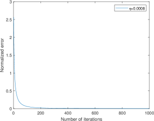
Figure 1: Convergence of GD

For the setting of unknown covariance matrices $Q$ and $R$, we use Algorithm 1 to compute $K_{t}^{*},t\in\mathbb{T}$ with $M=3$. Let initial policy $\mathbf{K}_{0}=0_{3\times 6}$, step size $\eta=0.0008$, number of iterations $V=4000$, and number of samples $L=200$. The numerical result is shown in Figure 2(a) and the average process of normalized estimation error over 10 simulations converges to $0$ around. If we set the number of samples $L$ be $2000$, the ultimate normalized estimation error and fluctuation range will be smaller as shown in Figure 2(b). This indicates that $\mathbf{K}_{k}$ will converge to $\mathbf{K}^{*}$ with enough samples.

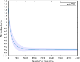
(a) $L=200$

(b) $L=2000$

Figure 2: The convergence of SGD over 10 simulations with different numbers of samples. The solid blue line is the average process of normalized estimation error over 10 simulations, and the shaded light blue area is the fluctuation range of normalized estimation error over 10 simulations.

Consider the scenario that $Q_{t}$ changes with time slowly

$$\delta Q=\begin{bmatrix}0.12&-0.08&0\\ -0.08&0.12&0\\ 0&0&0.05\\ \end{bmatrix},Q_{t}=\begin{bmatrix}0.61&-0.195&-0.3377\\ -0.195&0.775&-0.0953\\ -0.3377&-0.953&0.665\\ \end{bmatrix}+t*\delta Q,\leavevmode\nobreak\ \leavevmode\nobreak\ \leavevmode\nobreak\ t=0,\dots,M+N.$$

Set initial policy $\mathbf{K}_{0}=\{K^{0}_{0},K^{0}_{1},K^{0}_{2}\}=0_{3\times 6}$, step size $\eta=0.0008$, and number of iterations $V=4000$. Figure 3(a) and Figure 3(b) show that the average process of normalized estimation error over 10 simulations converges to $f(\mathbf{K}^{*})$ around with number of samples $L=200$ and $L=2000$, respectively. Comparing Figure 2 with 3, the estimation error in the setting of time-varying $Q_{t}$ is bigger than that in the setting of time-invariant $Q_{t}$.

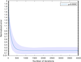
(a) $L=200$

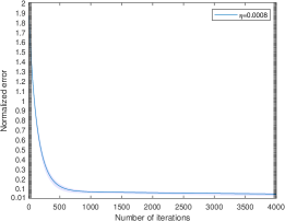
(b) $L=2000$

Figure 3: The convergence of SGD over 10 simulations with different numbers of samples with time-varying $Q_{t}$.

7 Conclusion

In this work, we consider to solve the finite-horizon KF problem with unknown noise covariance, which is reformulated as a policy optimization problem of the dual system. We provide the global convergence guarantee and sample complexity of the proposed SGD method. Our consideration might be viewed as a supplement to the adaptive filtering methodology. In the future, we will explore the finite-horizon KF problem and steady-state KF problem for more general systems.

References

- [1] Roland Hostettler, Wolfgang Birk, and Magnus Lundberg Nordenvaad. Extended kalman filter for vehicle tracking using road surface vibration measurements. In 2012 IEEE 51st IEEE Conference on Decision and Control (CDC), pages 5643–5648, 2012.
- [2] Tamer Mekky Ahmed Habib. Simultaneous spacecraft orbit estimation and control based on gps measurements via extended kalman filter. The Egyptian Journal of Remote Sensing and Space Science, 16(1):11–16, 2013.
- [3] Hadis Karimipour and Venkata Dinavahi. Extended kalman filter-based parallel dynamic state estimation. IEEE Transactions on Smart Grid, 6(3):1539–1549, 2015.
- [4] R. Clarke, J. Waddington, and J.N. Wallace. The application of kalman filtering to the load/pressure control of coal-fired boilers. In IEE Colloquium on Kalman Filters: Introduction, Applications and Future Developments, pages 2/1–2/6, 1989.
- [5] Jose A. Rosendo, Alfonso Bachiller, and Antonio Gomez. Application of self-tuned kalman filters to control of active power filters. In 2007 IEEE Lausanne Power Tech, pages 1262–1265, 2007.
- [6] Jaroslav Macalak. Application of kalman filtering to acoustic sound diagnostic measurement. In 13th Mechatronika 2010, pages 84–86, 2010.
- [7] M.R. Katebi and M.J. Grimble. Marine application of kalman filtering. In IEE Colloquium on Kalman Filters: Introduction, Applications and Future Developments, pages 3/1–3/3, 1989.
- [8] R. Mehra. Approaches to adaptive filtering. IEEE Transactions on Automatic Control, 17(5):693–698, 1972.
- [9] C. G. Hilborn and Demetrios G. Lainiotis. Optimal estimation in the presence of unknown parameters. IEEE Transactions on Systems Science and Cybernetics, 5(1):38–43, 1969.
- [10] R. E. Kalman. A New Approach to Linear Filtering and Prediction Problems. Journal of Basic Engineering, 82(1):35–45, 03 1960.
- [11] V.K. Kotti and A.G. Rigas. Identification of a stochastic neuroelectric system using the maximum likelihood approach. In 6th International Conference on Signal Processing, 2002., volume 2, pages 1492–1495 vol.2, 2002.
- [12] Patrick L. Smith. Estimation of the covariance parameters of non-stationary time-discrete linear systems. 1971.
- [13] K. Myers and B. Tapley. Adaptive sequential estimation with unknown noise statistics. IEEE Transactions on Automatic Control, 21(4):520–523, 1976.
- [14] C. Neethling and P. Young. Comments on "identification of optimum filter steady-state gain for systems with unknown noise covariances". IEEE Transactions on Automatic Control, 19(5):623–625, 1974.
- [15] B.J. Odelson, A. Lutz, and J.B. Rawlings. The autocovariance least-squares method for estimating covariances: application to model-based control of chemical reactors. IEEE Transactions on Control Systems Technology, 14(3):532–540, 2006.
- [16] Brian J. Odelson, Murali R. Rajamani, and James B. Rawlings. A new autocovariance least-squares method for estimating noise covariances. Automatica, 42(2):303–308, 2006.
- [17] Lingyi Zhang, David Sidoti, Adam Bienkowski, Krishna R. Pattipati, Yaakov Bar-Shalom, and David L. Kleinman. On the identification of noise covariances and adaptive kalman filtering: A new look at a 50 year-old problem. IEEE Access, 8:59362–59388, 2020.
- [18] Maryam Fazel, Rong Ge, Sham Kakade, and Mehran Mesbahi. Global convergence of policy gradient methods for the linear quadratic regulator. In Jennifer Dy and Andreas Krause, editors, Proceedings of the 35th International Conference on Machine Learning, volume 80 of Proceedings of Machine Learning Research, pages 1467–1476. PMLR, 10–15 Jul 2018.
- [19] Ben Hambly, Renyuan Xu, and Huining Yang. Policy gradient methods for the noisy linear quadratic regulator over a finite horizon. SIAM Journal on Control and Optimization, 59(5):3359–3391, 2021.
- [20] Hesameddin Mohammadi, Mahdi Soltanolkotabi, and Mihailo R. Jovanović. On the linear convergence of random search for discrete-time lqr. IEEE Control Systems Letters, 5(3):989–994, 2021.
- [21] Hesameddin Mohammadi, Armin Zare, Mahdi Soltanolkotabi, and Mihailo R. Jovanović. Convergence and sample complexity of gradient methods for the model-free linear–quadratic regulator problem. IEEE Transactions on Automatic Control, 67(5):2435–2450, 2022.
- [22] Feiran Zhao, Keyou You, and Tamer Başar. Global convergence of policy gradient primal–dual methods for risk-constrained lqrs. IEEE Transactions on Automatic Control, 68(5):2934–2949, 2023.
- [23] Yingying Li, Yujie Tang, Runyu Zhang, and Na Li. Distributed reinforcement learning for decentralized linear quadratic control: A derivative-free policy optimization approach. IEEE Transactions on Automatic Control, 67(12):6429–6444, 2022.
- [24] Kaiqing Zhang, Bin Hu, and Tamer Başar. Policy optimization for linear control with robustness guarantee: Implicit regularization and global convergence, 2021.
- [25] Xiangyuan Zhang, Bin Hu, and Tamer Başar. Learning the kalman filter with fine-grained sample complexity. In 2023 American Control Conference (ACC), pages 4549–4554, 2023.
- [26] Shahriar Talebi, Amir Hossein Taghvaei, and Mehran Mesbahi. Data-driven optimal filtering for linear systems with unknown noise covariances. ArXiv, abs/2305.17836, 2023.
- [27] Jack Umenberger, Max Simchowitz, Juan C. Perdomo, K. Zhang, and Russ Tedrake. Globally convergent policy search over dynamic filters for output estimation. ArXiv, abs/2202.11659, 2022.
- [28] P.A. Blackmore and R.R. Bitmead. Duality between the discrete-time kalman filter and lq control law. IEEE Transactions on Automatic Control, 40(8):1442–1444, 1995.
- [29] Omiros Papaspiliopoulos. High-dimensional probability: An introduction with applications in data science. Quantitative Finance, 20(10):100–101, 2020.