A distributed-memory parallel algorithm for discretized integral equations using Julia
Abstract
Boundary value problems involving elliptic PDEs such as the Laplace and the Helmholtz equations are ubiquitous in physics and engineering. Many such problems have alternative formulations as integral equations that are mathematically more tractable than their PDE counterparts. However, the integral equation formulation poses a challenge in solving the dense linear systems that arise upon discretization. In cases where iterative methods converge rapidly, existing methods that draw on fast summation schemes such as the Fast Multipole Method are highly efficient and well established. More recently, linear complexity direct solvers that sidestep convergence issues by directly computing an invertible factorization have been developed. However, storage and compute costs are high, which limits their ability to solve large-scale problems in practice. In this work, we introduce a distributed-memory parallel algorithm based on an existing direct solver named “strong recursive skeletonization factorization.” The analysis of its parallel scalability applies generally to a class of existing methods that exploit the so-called strong admissibility. Specifically, we apply low-rank compression to certain off-diagonal matrix blocks in a way that minimizes data movement. Given a compression tolerance, our method constructs an approximate factorization of a discretized integral operator (dense matrix), which can be used to solve linear systems efficiently in parallel. Compared to iterative algorithms, our method is particularly suitable for problems involving ill-conditioned matrices or multiple right-hand sides. Large-scale numerical experiments are presented to demonstrate the performance of our implementation using the Julia language.
I Introduction
Boundary value problems of classical potential theory appear frequently in scientific and engineering domains. Many such problems involving elliptic partial differential equations (PDEs), e.g., Laplace’s and the Helmholtz equations, can be formulated as integral equations of the form
| (1) |
where is derived from the free-space fundamental solution associated with the elliptic operator; where and are given functions; and where is the unknown. While it may be challenging to solve the original PDEs directly, the corresponding integral formulations offer several advantages (see, e.g., [1, Chapter 10]).
We are interested in solving a large dense linear system
| (2) |
that arises from the discretization of an integral equation. The structure that we exploit is that the matrix is associated with a set of points such that
| (3) |
The kernel function is typically singular at the origin but otherwise smooth. In this work, we restrict ourselves to the case that is not too oscillatory. An important consequence of eq. 3 is that certain off-diagonal blocks in can be compressed using low-rank approximations. In particular, the required numerical rank is constant (independent of ) for a prescribed accuracy when an off-diagonal block satisfies the so-called strong admissibility. This observation is crucial for the success of the fast multipole method (FMM) [2, 3], which requires only operations for applying matrix to a vector. It may be somewhat surprising that under mild assumptions motivated by numerical experiments, a factorization of can also be computed using operations [4, 5, 6, 7, 8]. Although the asymptotic complexity is appealing, such factorization algorithms still require a significant amount of computation and memory footprint. A natural solution is to distribute the required computation and storage across multiple compute nodes in order to solve large-scale problems. The challenge here comes from the fact that the matrix is dense, which seems to imply that the cost of communication among compute nodes may be excessive.
In this paper, we demonstrate that such a concern is not necessary. In particular, we show that the required communication is local in the sense that every compute node communicates with only its neighbors in a sparse graph. Such a result is related to the parallel scalability of the FMM, where every compute node stores a local essential tree with other compute nodes to exchange messages.
I-A Contributions
We introduce a distributed-memory parallel algorithm for solving dense linear systems that arise from the discretization of two-dimensional volume integral equations. Our algorithm has two phases: (1) a factorization phase that constructs an approximate factorization of the dense matrix subject to a prescribed accuracy and (2) a solution phase that applies the former factorization to any right-hand side (vector) and obtain an approximate solution. The advantage of our approach is that once the first phase finishes, the second phase is extremely efficient. Therefore, our algorithm is particularly suitable for solving the following two types of problems:
-
1.
The condition number of is large. This typically occurs when eq. 1 is a first-kind Fredholm integral equation for Laplace’s equation or the Stokes equation, which has applications in magnetostatics, electrostatics and fluid dynamics. For example, the condition number of scales empirically as for Laplace’s equation.
-
2.
Multiple right-hand sides need to be addressed. This typically occurs when eq. 1 is the Lippmann-Schwinger equation that models the scattering of acoustic waves in media with variable save speed, which has applications in seismology, ultrasound tomography, and sonar. To resolve multiple incident fields, we only need to compute the factorization of once before applying it to different right-hand sides.
Our parallel algorithm for factorizing matrix is based on an existing sequential method named strong recursive skeletonization (RS-S) [7]. But the analysis of data dependency and the parallelization strategy generally apply to a class of methods based on strong admissibility including RS-S, the inverse fast multipole method [4, 8] and the compress-and-eliminate solver [9, 10]. The fundamental step employed in these methods is the following: (1) the set of row/column indices is partitioned into clusters such that indices in the same cluster correspond to points close to each other in space; (2) given a cluster of indices , the off-diagonal submatrices and are compressed using low-rank approximations for a set of indices , the union of all clusters satisfying the strong admissibility condition.
We show that applying Gaussian elimination to a subset of indices in after the compression (a.k.a, skeletonization) leads to a Schur-complement update that affects only neighbors of , clusters adjacent to . In addition, the compression step for can be performed locally without forming the two big matrices entirely. Based on these observations, we propose a domain decomposition strategy where the computational domain is partitioned among all processors. So all processors work on their interior clusters in parallel. To process the remaining boundary clusters, we color all processors so any pair of processors have two different colors if they own adjacent clusters. Then, we loop over all colors, and processors with the same color can work in parallel at each iteration.
We implemented our parallel algorithm using the Julia programming language111https://julialang.org/ because of its ease of usage and support for various numerical linear algebra routines. In particular, our implementation explores the distributed computing capability of Julia222https://docs.julialang.org/en/v1/manual/distributed-computing/. To show the performance of our software, we present large-scale numerical results for solving (1) first-kind Fredholm integral equation for Laplace’s equation and (2) the Lippmann-Schwinger equation. For example, a dense matrix with 268 million rows/columns associated with the Laplace kernel can be factorized in 100 seconds using 1024 cores (see table I).
I-B Related work
Before discussing methods based on the strong admissibility, we mention two algorithms based on the weak admissibility proposed by Corona et al. [5] and Ho et al. [6], respectively. They improve upon earlier recursive skeletonization ideas [11, 12] by incorporating an extra compression step on intermediate skeletons. Assuming that the Schur complements during the elimination process in the original algorithms retain the same rank structure as matrix in eq. 2, the authors proved nearly linear complexities for corresponding methods.
Methods based on the strong admissibility have a clear advantage: they can reuse the quad-/oct-tree data structure from the FMM. Indeed, the inverse FMM method [4, 8] and the strong recursive skeletonization factorization [7] are closely related to the black-box FMM [13, 14] and the kernel-independent FMM [15, 16], respectively. As a consequence, they are relatively easy to deploy in practice, and they have been utilized for solving acoustic scattering problems [17], for solving Stokes flow in porous media [18], and for solving electromagnetic scattering from large complex perfect conduct problems [19] and from homogeneous penetrable objects [20]. The strong recursive skeletonization factorization has also been coupled with high-order quadrature schemes for multiscale boundary integral equations in three dimensions recently [21]. Again, assuming the numerical ranks are constant for well-separated interactions (off-diagonal blocks satisfying the strong admissibility) in the Schur complements during an elimination process, both the inverse FMM and the strong recursive skeletonization factorization can be shown to achieve linear complexity (albeit with somewhat large constants).
Our goal of this paper is to demonstrate the parallel scalability of methods based on strong-admissibility for solving dense linear systems on distributed-memory machines. The two most related methods are as follows: Ma et al. [22] proposed a distributed-memory parallel algorithm for solving eq. 2 in two passes, where the first pass precomputed necessary information in order to gain parallelism in the second pass. Takahashi et al. [23] proposed a parallel algorithm of the inverse FMM for shared-memory machines. Other related work includes the following. Grama et al. [24] introduced parallel hierarchical solvers and preconditioners for boundary element methods. Rouet et al. [25] introduced a distributed-memory parallel algorithm for the so-called HSS matrix based on weak admissibility that generally leads to larger numerical ranks. Ghysels et al. [26] introduced a multicore implementation based on an HSS-structured multifrontal solver using randomized sampling. Yu et al. [27] introduced distributed linear-time solver for dense symmetric hierarchical semi-separable matrices. Cao et al. [28] introduced a parallel algorithm based on the tile low-rank format and demonstrated its performance on large-scale covariance matrices used in geostatistical modeling.
II Sequential algorithm and data dependency
In this section, we review the sequential algorithm for factorizing and solving eq. 2 approximately. The focus here is analyzing data dependency and parallelism. While there exist a few methods that are closely related such as [4, 8, 9, 10], we mostly follow [7, 21].
Suppose we are given a set of points in and a kernel function that defines matrix as in eq. 3. Our approach for solving eq. 2 employs approximate Gaussian elimination in a multi-level fashion.
II-A Hierarchical domain decomposition
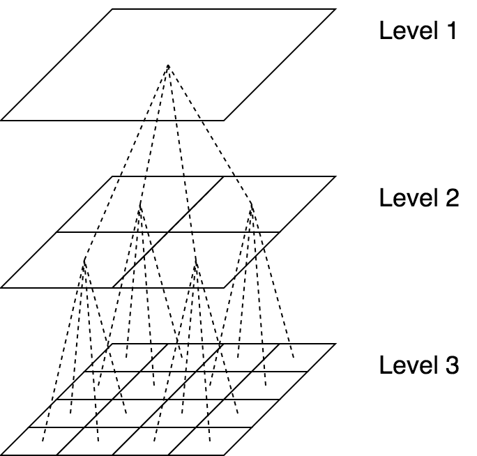
The algorithm relies on a hierarchical decomposition of the points as in the FMM. The hierarchical decomposition is as follows. Suppose all points lie in a square domain. We divide the domain into four equal-sized subdomains. We call the entire domain the parent of the four subdomains, which are the children of the original domain. We continue subdividing the four subdomains recursively until every subdomain contains points. This hierarchical decomposition of the problem domain naturally maps to a quad tree , where the root is the entire domain and the leaves are all subdomains that are not subdivided. See a pictorial illustration in fig. 1(a).
For ease of presentation, we further make the assumption that the points are uniformly distributed, so the hierarchical domain decomposition corresponds to a perfect quad tree (all internal nodes have 4 children and all the leaf nodes are at the same level). Extensions to a non-uniform distribution of points are straightforward; see details in [7, 21].
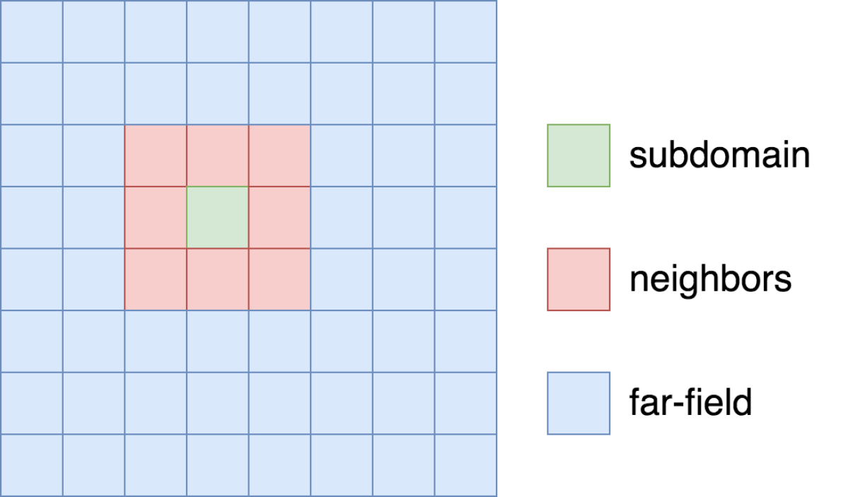
We refer to a subdomain (or a node in tree ) as a box for the rest of this paper. Given a box at level in the tree , its parent and its children are naturally defined (if they exist). We also define the near-field (a.k.a., neighbors) and the far-field as follows:
-
•
: boxes that are physically adjacent to (excluding ) at level .
-
•
: boxes excluding at level .
See an example in fig. 1(b). Assuming is a perfect quad-tree, it is obvious that no box has more than eight neighbors, i.e., . In the following, we abuse notations and use to also denote indices of points in that are contained in box , its near-field/neighbors , and its far-field , respectively.
Given a leaf node , there exists a permutation matrix such that
| (4) |
Here, for two index sets and stands for the corresponding submatrix in .
II-B Low-rank property
Assumption 1
For any box , it holds that for (1) and ; or (2) and . In other words, the submatrices and come from kernel evaluation.
The observation is that the off-diagonal block (or ) for an arbitrary box can be approximated efficiently by a low-rank approximation for a prescribed accuracy . In particular, the numerical rank is , independent of the problem size , for a smooth kernel that is not highly oscillatory.
Next, we explain a specific type of low-rank approximation named the interpolative decomposition (ID) [29], which is applied to the submatrix . Other low-rank approximations such as the truncated singular value decomposition can also be used; see the resulting solvers for eq. 2 in, e.g., [9, 30].
Definition 1
Let and be the row and column indices of a matrix . A (column) interpolative decomposition (ID) for a prescribed accuracy finds the so-called skeleton indices , the redundant indices , and an interpolation matrix such that
While the strong rank-revealing QR factorization of Gu and Eisenstat [31] is the most robust method for computing an ID, we employ the column-pivoting QR factorization as a greedy approach [29], which has better computational efficiency and behave well in practice. In particular, we adopted the implementation from the LowRankApprox.jl333https://github.com/JuliaLinearAlgebra/LowRankApprox.jl package. The cost to compute an ID using the aforementioned deterministic methods is , which can be further reduced to using randomized algorithms that may incur some loss of accuracy [32].
II-C Fast compression
As stated earlier, we want to compress the two off-diagonal blocks and using their IDs. In practice, we conduct one (column) ID compression of the concatenation
| (5) |
(that has rows and columns) and obtain a single interpolation matrix that satisfies both
| (6) |
This approach leads to a slightly larger set of skeleton indices but makes the algorithm/implementation easier.
Notice that the computational cost would be if the full matrix in eq. 5 is formed, which turns out to be unnecessary. As in the FMM, there are a few techniques that require only operations such as the (analytical) multipole expansion (see, e.g., [2, 3, 33]), the Chebyshev interpolation (see, e.g., [13, 14]), and the proxy method (see, e.g., [15, 11]).
Below, we focus on illustrating the proxy method for compressing the submatrix . Specifically, we form and compress the following matrix
| (7) |
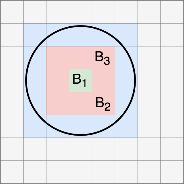
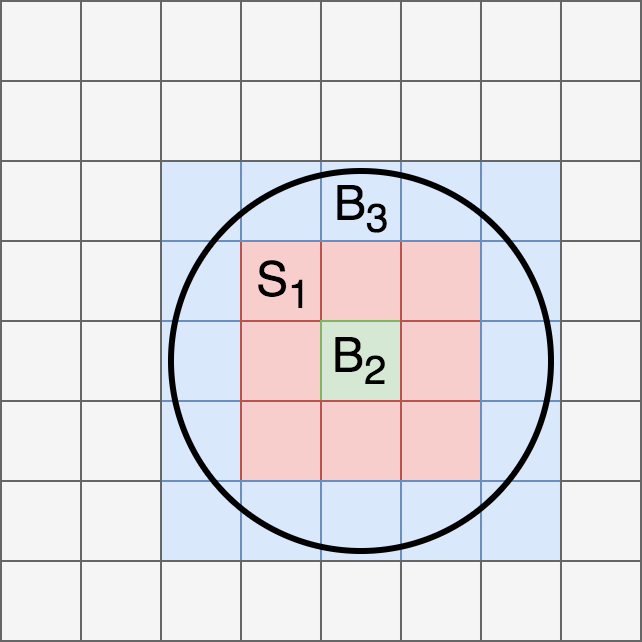
which has rows (and columns). In eq. 7, is a small subset of surrounding defined as follows (see fig. 2):
Definition 2
The distance-2 neighbors of a box is defined as
Note that 1 does not hold in our algorithm, where the submatrix is updated and is not the kernel evaluation any more; see section II-D. However, we can show the following to be true:
Theorem 1
For any leaf box , it holds that for (1) and ; or (2) and . In other words, the submatrices and come from kernel evaluation.
This relaxation means that the established rank estimation in section II-B no longer holds. However, we empirically verify that the resulting rank from compressing eq. 7 still follows the previous estimation; see numerical results in section V.
In eq. 7, stands for a matrix where the -th entry is given by , i.e., a kernel evaluation between a discretization point on the proxy circle444A circle is chosen for ease of implementation but not necessary mathematically. and a point lying inside the box . The “interaction” accounts for the “interaction” between points lying in and points inside . To that end, the proxy circle must lie inside . See a pictorial illustration in fig. 2. In this paper, we choose the radius of the proxy circle to be , where is the side length of boxes at this level.
Remark 1
The computation of skeleton indices , redundant indices , and the interpolation matrix in eq. 6 requires (reads) submatrices and (not the entire submatrices or ) for a leaf box .
II-D Approximate matrix factorization
The algorithm starts at the leaf level of the quad-tree . Let us apply an ID compression for a box to obtain skeleton indices , redundant indices , and an interpolation matrix such that eq. 6 holds. (As explained in the previous section, this step requires only operations.)
Rewrite eq. 4 as
where is an appropriate permutation matrix. Define the sparsification matrix
| (8) |
where the partitioning of row and column indices is the same as that of and the diagonal blocks are identity matrices of appropriate sizes. Applying the sparsification matrix, we have that
where the coupling (submatrices) between and disappears. Here, the notation denotes modified blocks that can be easily derived and be calculated using operations. Notice that we never need to explicitly form or .
Suppose that the diagonal block is non-singular and that is an LU factorization. We apply (block) Gaussian elimination to obtain
| (9) |
where
Notice that the original “interaction” among ’s neighbors, i.e., submatrix , has been updated.
Define
| (10) |
Here, is called the strong skeletonization operator in [7]. Note that and can be applied efficiently without explicitly forming their inverses.
Remark 2
Given the interpolation matrix in eq. 6, applying the strong skeletonization operator requires (reads) matrices and , and it updates (read & write) submatrix for a leaf box . (No far-field information is required.)
II-E Multi-level algorithm
Let denote the number of boxes at level in the quad-tree (). Given an ordering of all boxes at the leaf level, our algorithm applies the strong skeletonization operator eq. 10 to all boxes one after another:
The resulting (approximate) factorization becomes
| (11) |
where the leading diagonal blocks are identity matrices of sizes , which correspond to the redundant indices in box for . The (approximate) Schur complement has rows and columns.
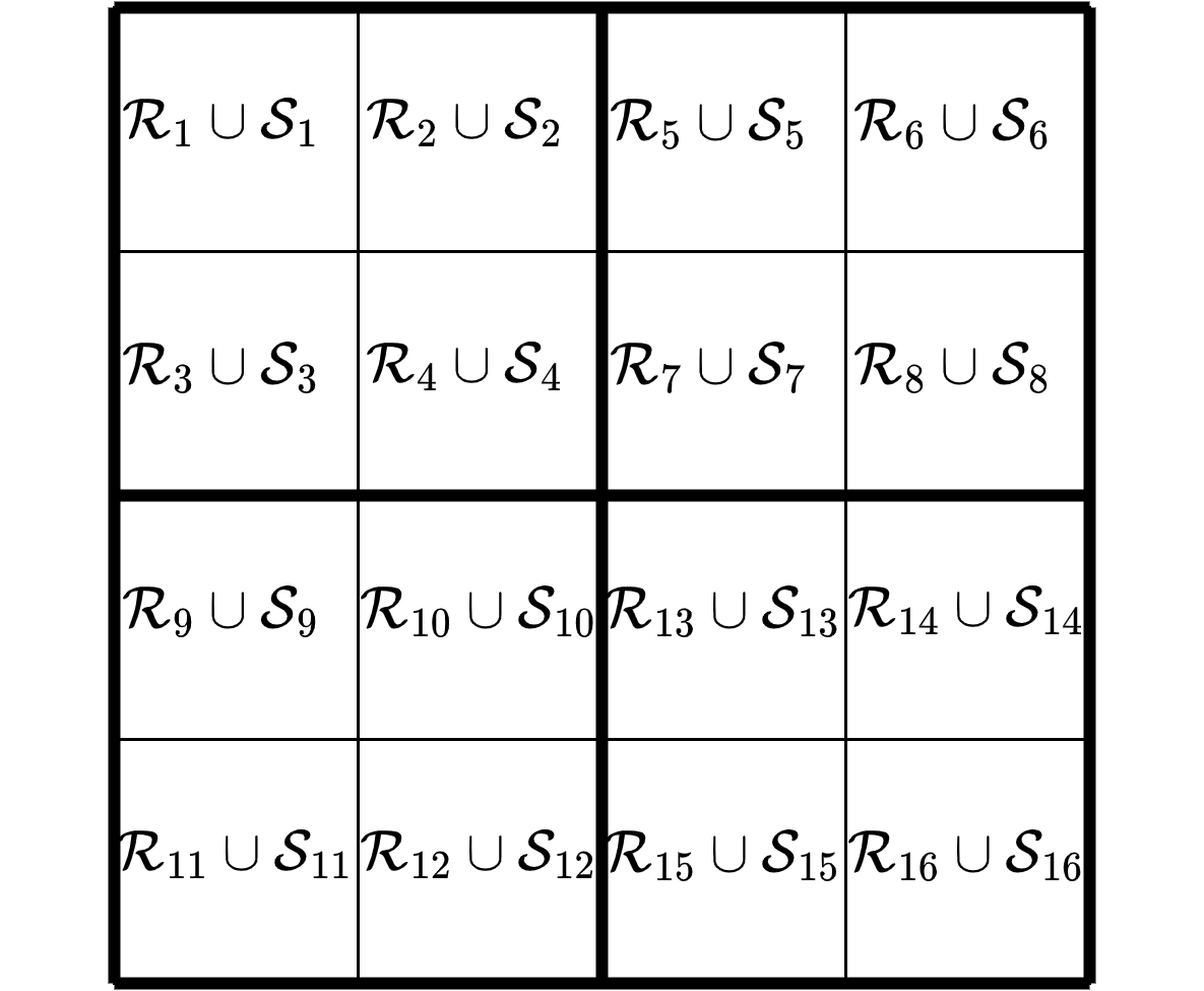
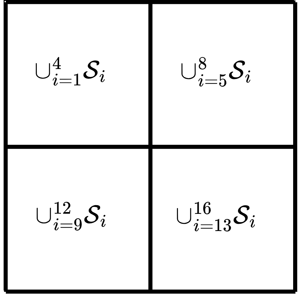
Next, we demonstrate that the single-level algorithm eq. 11 can be applied to recursively. In order to factorize (approximately), we consider the remaining skeleton points at the coarse level . Let every box own the skeleton points of its children, i.e., . See fig. 3 for a pictorial illustration. We obtain a partitioning of as we did for (a leaf box owns points physically lying inside it).
In order to continue applying the strong skeletonization operator to every box at level , we need to first verify 1 still holds. For the skeletons in box , the modified interactions (submatrices) only exist between and . At level , it can be shown that the parent of is the neighbor of the parent of any box in . As a result, 1 holds, and thus we can repeat the previous approach to apply the strong skeletonization operator to every box at level . By induction, we know that
Theorem 2
1 holds at all levels 555There is no far-field for any box at level 1, so the theorem holds trivially..
We refer to [7, Section 3.3.2] for a formal proof of the above theorem. The implication of the theorem is that remark 2 and remark 1 both hold at all levels. Therefore, we obtain a multi-level algorithm:
| (12) |
As explained in section II-D, the inverse of a strong skeletonization operator can be applied efficiently (without forming the inverse operator explicitly). We summarize the complete algorithm in algorithm 1.
As mentioned earlier, other low-rank approximation methods can also be used to construct similar factorizations [4, 8]. The same framework can be applied to solving large sparse linear systems with minor modifications [9, 10]. While the described framework leverages the so-called strong admissibility (compression of far-field), a few methods based on the weak admissibility (compression of both far-field and near-field) can also construct efficient factorizations [5, 6].
II-F Solution/applying the inverse of factorization
The solution phase follows the standard forward and backward substitution procedures besides applying the inverse of the sparsification operator eq. 8. The algorithm consists of an upward and a downward level-by-level traversal of the tree . During the upward pass, all boxes at the same level are visited according to the order of factorization. For every box , we first update a subset of the right-hand-side (RHS) and then update associated with neighbor boxes of in our in-place algorithm. The operations are “reversed” during the downward pass, where we read neighbor data and update local data for every box .
III Distributed-memory parallel algorithm
In the following, we analyze data dependency at the leaf level based on previous results summarized in remarks 1 and 2, but the analysis also holds at other levels in the tree (see section II-E). In Julia, a master process (process 1) provides the interactive prompt and coordinates worker processes to conduct parallel operations. To store our data structures such as a list of required submatrices for every box, we used distributed arrays from DistributedArrays.jl. A distributed array has the property that a process can make a fast local access but has only read permission for a remote access. Our parallel algorithm starts by constructing local data structures on each worker and assembling them into distributed arrays.
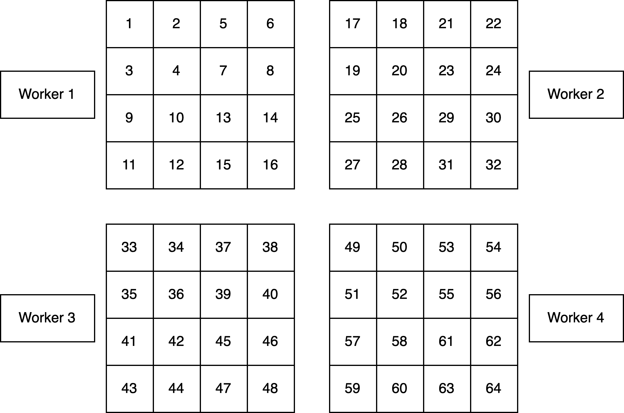
At the leaf level, all boxes are distributed evenly among all worker processes. See fig. 4 for an example. On every worker , the boxes are classified into two groups: (1) “interior boxes”, whose neighbors are on the same worker, and (2) “boundary boxes”, whose neighbors are on and at least one other worker . In fig. 4, boundary boxes on worker 1 include 6, 8, 14, 16, 11, 12, and 15; and the rest are all interior boxes. Notice that if the total number of boxes is large, the number of interior boxes dominates.
Consider a pair of boxes and at the leaf level. Suppose the two boxes are on two different workers and , respectively. (Otherwise, the two boxes will be processed sequentially.) Consider the distance between the two boxes,666, where and are the centers of and , respectively, and is the side length of boxes at the same level as and . where
-
1.
if and are neighbors/adjacent (e.g., boxes 6 and 17 in fig. 4). In fact, both boxes must be boundary boxes. We discuss the parallel algorithm for handling all boundary boxes in section III-B.
-
2.
if and are not neighbors but share a common neighbor, i.e., they are distance-2 neighbors as defined in definition 2 (e.g., boxes 5 and 17 in fig. 4). In fact, one of the two boxes must be a boundary box and the other one must be an interior box. If one of them, say , is processed first, it requires accessing the corresponding submatrices and (see remark 1) but will not update submatrices in the rows/columns of (see remark 2).
- 3.
Our parallel algorithm for the described matrix factorization employs a level-by-level traversal of the quad-tree . At every level, we have three steps: (1) processing the massive interior boxes in parallel, (2) processing the remaining boundary boxes, and (3) creating the next/coaser level. The pseudocode is shown in algorithm 2, and we explain implementation details in the following sections.
III-A Interior boxes
For the first step in our parallel algorithm at every level, notice that if a pair of interior boxes and are on two different workers, then (e.g., boxes 5 and 18 in fig. 4). Therefore, all workers can apply the strong skeletonization operator (see algorithm 1) to factorize their respective interior boxes concurrently. In our implementation, every worker stores all necessary submatrices for this step. For example, in fig. 4 both worker 1 and worker 2 store copies of the submatrices and . Recall remark 1 that both box 5 and box 17 need the two submatrices for computing their IDs.
The syntactical structure of our implementation is similar to task-based programming, in which the master process launches the factorization tasks to all workers through a for loop:
Here, remotecall_wait tells worker to factorize a set of boxes, the async macro means the task launch is asynchronous, and the sync macro on the loop makes sure that the master process waits for all workers to finish their tasks. (If remotecall is used instead, then the master process only waits for all workers to receive their tasks.)
III-B Boundary boxes
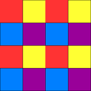
After the first step, all workers are left with their boundary boxes to be processed. We assign colors to all workers such that any pair of adjacent processes have two different colors. Although mature software packages exist for coloring an arbitrary graph, we assume the boxes at every level form a grid (a full quad-tree ), and thus a coloring of the process grid is straightforward as shown in fig. 5. Notice that 4 colors are needed for a 2D process grid regardless of the number of boxes on every worker.
Once the coloring is available, our parallel algorithm loops over all colors. For each color, the associated processors need to fetch submatrices required for subsequent computation and then process their boundary boxes in parallel. For the example in fig. 5, our algorithm will schedule 4 boxes, say with red color; wait for their completion; then schedule the next 4 boxes, say with yellow color; wait for their completion; and so on. Notice that if a pair of boundary boxes and are on two different processors with the same color, then as long as every processor has at least boxes.
After all workers with a specific color finish factorizing their boundary boxes, they need to send submatrices from Schur complement updates to their neighbors. In Julia, communication is “one-sided,” which means that only one process needs to be explicitly managed by the programmer. According to our best knowledge, remote direct memory access [34] is not available in Julia for distributed computing. So we implemented explicit communication through remote procedural calls. In particular, the master process launches receive_data tasks on the neighbor workers as follows:
Here, receive_data is a function defined on all workers through the use of the everywhere macro as follows:
where the worker that needs data launches tasks on its neighbors who have color , and data will be returned in the form of a future object. Finally, the neighbor with color returns/sends the requested data back, which is stored in a distributed array.
III-C Level transition
Since the algorithm traverses the quad-tree in a level-by-level fashion starting from the leaf level, it is important to keep track of the data structure when the algorithm transitions from one level to the next. The approach we take is to explicitly store the modified interactions for every box. As a result, whenever the algorithm changes level, it will need to reconstruct the data structure by regrouping interactions among accumulated points. An additional thing that we need to keep track of is where the coordinates of the given points are stored. At the start of the algorithm, the points are stored evenly distributed across all processes using a distributed array. However, as the algorithm progresses from one level to the next, two things will change. First, since each new level are constructed from the skeletonized points of the previous level, the points that are involved in the factorization of the new level are a subset of the previous points. Second, the number of processes involved in the new level may also decrease. Hence, this suggests that during the transition stage, we also need to reconstruct a distributed array by using only the relevant skeletonized points.
IV Complexity analysis
We assume that the number of points per box at the leaf level is , where is the numerical rank that stays constant regardless of the problem size . Furthermore, we let be the number of levels of the quad-tree .
IV-A Computational and memory complexity
The costs of the strong RS algorithm were derived in [7, Section 3.3.4]: the factorization cost , the solve cost , and the memory footprint also scales as , where is the problem size. Similar results for the inverse FMM algorithm can be found in [8, Section 2.5]. In the parallel algorithm, we uniformly partition the problem, the required work, and the memory footprint among all processors.
IV-B Communication cost
Notice the quad-tree has levels, and all processors are organized as another quad-tree with levels. So every processor owns a subtree of levels. In our parallel factorization algorithm, every processor sends a constant number of messages with a constant number of words for the first levels. Then, the remaining algorithm behaves as a parallel reduction among processors. As a result, the number of messages sent by every processor is , and the number of words moved is
| (13) |
where is the number of boundary boxes on every processor. For strong scaling experiments (), we obtain
For weak scaling experiments (), we obtain:
V Numerical results
In this section, we show benchmark results for solving two types of dense linear systems that are induced by the free-space Green’s function for the Laplace equation in 2D and that for the Helmholtz equation in 2D, respectively. They represent kernel functions that are non-oscillatory and mildly oscillatory. The accuracy of our approximate factorization is controlled by , the relative error in the ID (see definition 1). In the experiments, we fixed and obtained high-quality preconditioners, which required only a few steps of preconditioned CG or GMRES to reach a tolerance of for solving the corresponding linear systems. For ease of setting up the experiments, we chose the point set to be uniform grids in the unit square, so the matrix-vector product with the dense linear operator could be performed efficiently via the fast Fourier transform. (Otherwise, a fast summation algorithm such as the distributed-memory fast Multipole Method is required.) Below are the notations we used to report results of our experiments (timings are in seconds):
-
•
: problem size/matrix size/number of points;
-
•
: number of processes used;
-
•
: time of constructing our factorization;
-
•
: time of applying the factorization once;
-
•
: number of preconditioned CG (PCG) or GMRES iterations for solving a single right-hand side (RHS) with tolerance .
All experiments were performed with Julia (version 1.7.3) on the CPU nodes of Perlmutter777https://docs.nersc.gov/systems/perlmutter/architecture/, an HPE (Hewlett Packard Enterprise) Cray EX supercomputer. Each compute node has two AMD EPYC 7763 (Milan) CPUs (64 cores per CPU) and 512 GB of memory. Since Julia employs a just-in-time compiler that compiles a code before its first execution, we always ran a small problem size before timing our numerical experiments. We also turned off the garbage collection Julia during the factorization stage for faster execution.
V-A Laplace kernel
Consider the following problem involving the free-space Green’s function for the 2D Laplace equation: solving the first-kind volume integral equation
| (14) |
where the kernel function . We discretized eq. 14 using piecewise-constant collocation on a uniform grid . The resulting linear system involves a dense matrix defined as follows: the off-diagonal entries are
| (15) |
where and and is the grid spacing; and the diagonal entries are given by
| (16) |
where , and and we evaluate eq. 16 numerically using an adaptive quadrature (dblquad from MultiQuad.jl).
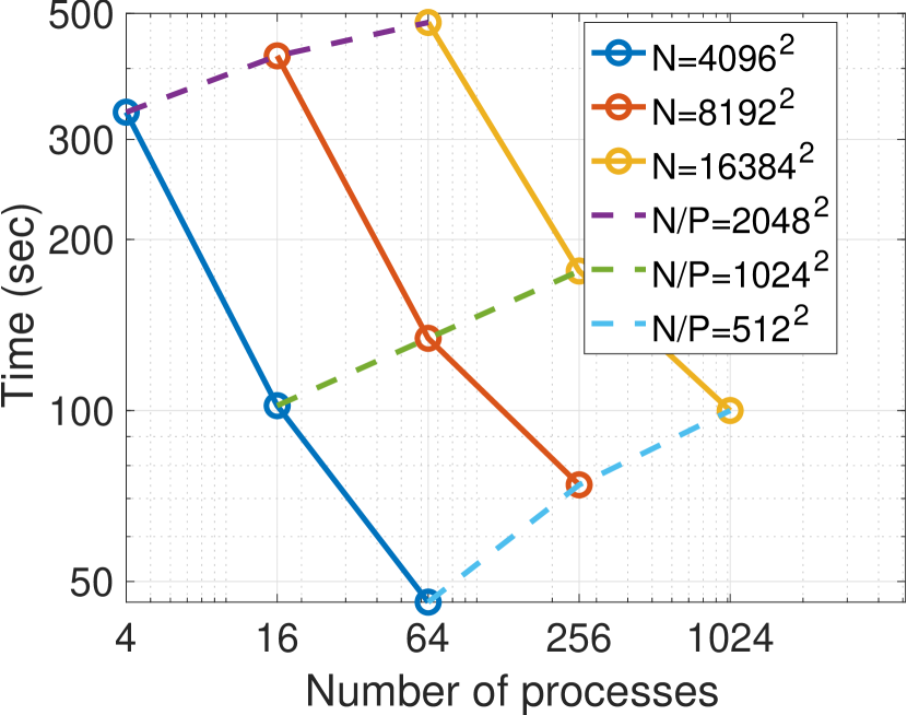
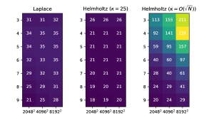
table I shows the relevant numerical results, and fig. 6 shows the parallel scalability of the factorization and the solve time. We make the following observations:
-
1.
We were able to solve a large problem size of million using 1024 processes in less than three minutes (100 seconds for factorization and around seconds for five PCG iterations).
-
2.
The approximate factorizations constructed in parallel required a consistent number (five) of PCG iterations to arrive at a tolerance of . By contrast, the number of CG iterations is approximately without any preconditioners.
-
3.
The solve time for a single RHS is much smaller than the factorization time. The speedup of the solve time is typically more than that of the factorization time because the solve phase requires less communication.
| factorization time | solve time (one iteration) | ||||||||
| 1 | 234 | 154 | 80 | 6.15 | 5.65 | 0.50 | |||
| 4 | 71 | 54 | 17 | 3.01 | 2.51 | 0.51 | |||
| 16 | 24 | 20 | 4 | 0.84 | 0.64 | 0.20 | |||
| 4 | 335 | 193 | 142 | 14.73 | 12.77 | 1.96 | |||
| 16 | 102 | 59 | 43 | 4.30 | 2.99 | 1.31 | |||
| 64 | 46 | 23 | 23 | 1.40 | 1.00 | 0.40 | |||
| 16 | 421 | 210 | 211 | 20.02 | 15.07 | 4.95 | |||
| 64 | 134 | 70 | 64 | 6.61 | 4.22 | 2.39 | |||
| 256 | 74 | 30 | 44 | 2.34 | 1.52 | 0.82 | |||
| 64 | 482 | 230 | 252 | 25.81 | 17.03 | 8.78 | |||
| 256 | 176 | 76 | 100 | 10.38 | 5.26 | 5.12 | |||
| 1024 | 100 | 38 | 62 | 7.25 | 3.64 | 3.61 | |||
V-B Helmholtz Kernel
Consider the next problem involving the free-space Green’s function for the 2D Helmholtz equation: solving the second-kind volume integral equation
| (17) |
where , known as the Lippmann-Schwinger equation, a reformulation of the variable coefficient Helmholtz equation (see, e.g., [1, Section 11.2]) that models, e.g., acoustic wave propagation in a medium with a variable wave speed. Here is the incoming wave with frequency ; the “scattering potential” is a known smooth function compactly supported inside ; and the kernel function where is the Hankel function of the first kind of order zero.
We can use the change of variable to symmetrize eq. 17 and then discretize using piecewise-constant collocation on a uniform grid . The resulting complex linear system involves a dense matrix defined as follows: the off-diagonal entries are
| (18) |
where and , and is the grid spacing; and the diagonal entries are given by
| (19) |
where , and we evaluate eq. 19 numerically using an adaptive quadrature (dblquad from MultiQuad.jl).
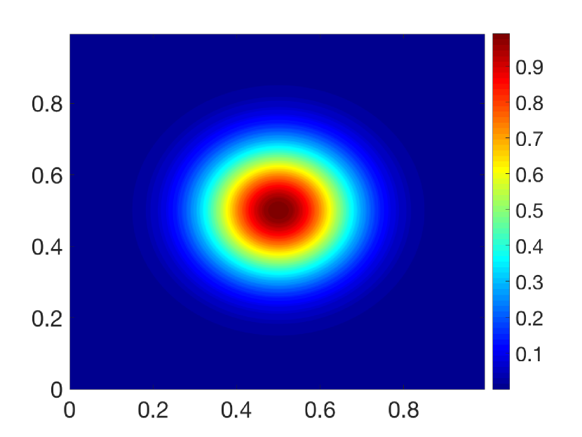
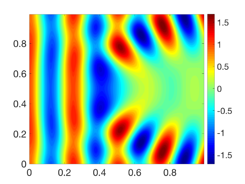
For the following experiments, we use a Gaussian bump scattering potential with the center , as shown in fig. 7(a). For an incoming plan wave pointing to the right, the total field is shown in fig. 7(b).
V-B1 Fixed frequency ()
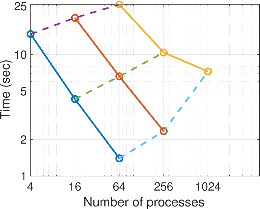
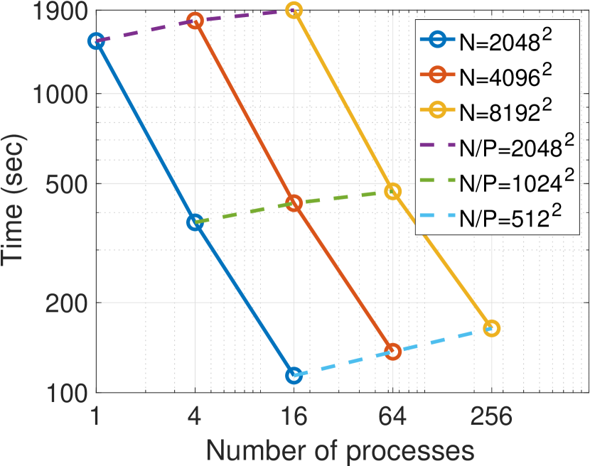
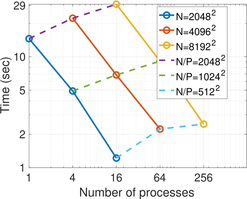
table II shows the relevant numerical results for a fixed frequency , and fig. 7 shows the parallel scalability of the factorization and the solve time. We make the following observations:
-
1.
The factorization time is much longer than that for the Laplace kernel. The major difference is that an evaluation of the (complex) Helmholtz kernel in LABEL:e:helmholtz takes longer.
-
2.
As a result of the significant computational costs for kernel evaluations, the parallel factorization algorithm achieves greater speedups compared to those for the Laplace kernel. In addition, one advantage of constructing a highly accurate approximation is clear: the solve time is much faster, suitable for situations where multiple RHSs need to be addressed.
-
3.
Again, the approximate factorizations constructed in parallel required a consistent number (three) of GMRES iterations to arrive at a tolerance of (when the frequency is fixed).
| factorization time | solve time (one iteration) | ||||||||
| 1 | 1499 | 1182 | 318 | 14.56 | 13.61 | 0.95 | |||
| 4 | 371 | 287 | 85 | 4.91 | 4.15 | 0.76 | |||
| 16 | 114 | 86 | 28 | 1.22 | 0.97 | 0.25 | |||
| 64 | 60 | 39 | 21 | 0.79 | 0.51 | 0.28 | |||
| 4 | 1754 | 1240 | 514 | 22.26 | 19.53 | 2.73 | |||
| 16 | 430 | 302 | 128 | 6.85 | 5.17 | 1.67 | |||
| 64 | 137 | 96 | 41 | 2.23 | 1.68 | 0.55 | |||
| 256 | 75 | 44 | 31 | 1.50 | 0.90 | 0.60 | |||
| 16 | 1901 | 1269 | 632 | 29.74 | 23.76 | 5.98 | |||
| 64 | 471 | 328 | 142 | 9.13 | 6.14 | 2.99 | |||
| 256 | 164 | 101 | 64 | 2.47 | 1.60 | 0.87 | |||
| 1024 | 101 | 54 | 47 | 5.36 | 1.75 | 3.61 | |||
V-B2 Increasing frequency (, i.e., 32 points per wavelength)
table III shows the relevant numerical results for incoming waves with increasing frequencies. We make the following observations:
- 1.
-
2.
As increases in eq. 17, the integral equation becomes increasingly more ill-conditioned. So is the discretized linear system, which requires more and more preconditioned GMRES iterations to converge. However, the savings from employing the preconditioner is clear: the number of GMRES iterations without any preconditioner is orders-of-magnitudes larger and grows rapidly.
| 1 | 32 | 365 | 1.83 | 3 | 452 | |||
| 4 | 64 | 495 | 14.56 | 4 | 1752 | |||
| 16 | 128 | 684 | 22.26 | 5 | 8198 | |||
| 64 | 256 | 1138 | 29.74 | 12 | - |
VI Conclusions and generalizations
In this paper, we have introduced a distributed-memory parallel algorithm based on the sequential RS-S method [7] for factorizing discretized two-dimensional volume integral equations. Our algorithm follows from an analysis of the data dependency of methods based on strong admissibility, among which RS-S is an example. We implemented the new algorithm using Julia and have presented large-scale numerical experiments to demonstrate its parallel scalability.
Several important future research directions include (1) implementation of adaptive domain decomposition, (2) incorporating high-order discretization schemes, and (3) extension to solving boundary integral equations in three dimensions.
References
- [1] P.-G. Martinsson, Fast direct solvers for elliptic PDEs. SIAM, 2019.
- [2] L. Greengard and V. Rokhlin, “A fast algorithm for particle simulations,” Journal of computational physics, vol. 73, no. 2, pp. 325–348, 1987.
- [3] ——, “A new version of the fast multipole method for the Laplace equation in three dimensions.” YALE UNIV NEW HAVEN CT DEPT OF COMPUTER SCIENCE, Tech. Rep., 1996.
- [4] S. Ambikasaran and E. Darve, “The inverse fast multipole method,” arXiv preprint arXiv:1407.1572, 2014.
- [5] E. Corona, P.-G. Martinsson, and D. Zorin, “An O(N) direct solver for integral equations on the plane,” Applied and Computational Harmonic Analysis, vol. 38, no. 2, pp. 284–317, 2015.
- [6] K. L. Ho and L. Ying, “Hierarchical interpolative factorization for elliptic operators: integral equations,” Comm. Pure Appl. Math, vol. 69, no. 7, pp. 1314–1353, 2016.
- [7] V. Minden, K. L. Ho, A. Damle, and L. Ying, “A recursive skeletonization factorization based on strong admissibility,” Multiscale Modeling & Simulation, vol. 15, no. 2, pp. 768–796, 2017.
- [8] P. Coulier, H. Pouransari, and E. Darve, “The inverse fast multipole method: using a fast approximate direct solver as a preconditioner for dense linear systems,” SIAM Journal on Scientific Computing, vol. 39, no. 3, pp. A761–A796, 2017.
- [9] H. Pouransari, P. Coulier, and E. Darve, “Fast hierarchical solvers for sparse matrices using extended sparsification and low-rank approximation,” SIAM Journal on Scientific Computing, vol. 39, no. 3, pp. A797–A830, 2017.
- [10] D. A. Sushnikova and I. V. Oseledets, ““compress and eliminate” solver for symmetric positive definite sparse matrices,” SIAM Journal on Scientific Computing, vol. 40, no. 3, pp. A1742–A1762, 2018.
- [11] P.-G. Martinsson and V. Rokhlin, “A fast direct solver for boundary integral equations in two dimensions,” Journal of Computational Physics, vol. 205, no. 1, pp. 1–23, 2005.
- [12] L. Greengard, D. Gueyffier, P.-G. Martinsson, and V. Rokhlin, “Fast direct solvers for integral equations in complex three-dimensional domains,” Acta Numerica, vol. 18, pp. 243–275, 2009.
- [13] W. Fong and E. Darve, “The black-box fast multipole method,” Journal of Computational Physics, vol. 228, no. 23, pp. 8712–8725, 2009.
- [14] R. Wang, C. Chen, J. Lee, and E. Darve, “PBBFMM3D: a parallel black-box algorithm for kernel matrix-vector multiplication,” Journal of Parallel and Distributed Computing, vol. 154, pp. 64–73, 2021.
- [15] L. Ying, G. Biros, and D. Zorin, “A kernel-independent adaptive fast multipole algorithm in two and three dimensions,” Journal of Computational Physics, vol. 196, no. 2, pp. 591–626, 2004.
- [16] P.-G. Martinsson and V. Rokhlin, “An accelerated kernel-independent fast multipole method in one dimension,” SIAM Journal on Scientific Computing, vol. 29, no. 3, pp. 1160–1178, 2007.
- [17] T. Takahashi, P. Coulier, and E. Darve, “Application of the inverse fast multipole method as a preconditioner in a 3d helmholtz boundary element method,” Journal of Computational Physics, vol. 341, pp. 406–428, 2017.
- [18] B. Quaife, P. Coulier, and E. Darve, “An efficient preconditioner for the fast simulation of a 2d stokes flow in porous media,” International Journal for Numerical Methods in Engineering, vol. 113, no. 4, pp. 561–580, 2018.
- [19] Z. Rong, M. Jiang, Y. Chen, L. Lei, X. Yang, and J. Hu, “Strong admissibility skeletonization factorization for fast direct solution of electromagnetic scattering from conducting objects,” IEEE Transactions on Antennas and Propagation, vol. 69, no. 10, pp. 6607–6617, 2021.
- [20] M. Jiang, Z. Rong, X. Yang, L. Lei, P. Li, Y. Chen, and J. Hu, “Analysis of electromagnetic scattering from homogeneous penetrable objects by a strong skeletonization-based fast direct solver,” IEEE Transactions on Antennas and Propagation, 2022.
- [21] D. Sushnikova, L. Greengard, M. O’Neil, and M. Rachh, “Fmm-lu: A fast direct solver for multiscale boundary integral equations in three dimensions,” arXiv preprint arXiv:2201.07325, 2022.
- [22] Q. Ma, S. Deshmukh, and R. Yokota, “Scalable linear time dense direct solver for 3-d problems without trailing sub-matrix dependencies,” in Proceedings of the International Conference on High Performance Computing, Networking, Storage and Analysis, ser. SC ’22. IEEE Press, 2022.
- [23] T. Takahashi, C. Chen, and E. Darve, “Parallelization of the inverse fast multipole method with an application to boundary element method,” Computer Physics Communications, vol. 247, p. 106975, 2020.
- [24] A. Grama, V. Kumar, and A. Sameh, “Parallel hierarchical solvers and preconditioners for boundary element methods,” SIAM Journal on Scientific Computing, vol. 20, no. 1, pp. 337–358, 1998.
- [25] F.-H. Rouet, X. S. Li, P. Ghysels, and A. Napov, “A distributed-memory package for dense hierarchically semi-separable matrix computations using randomization,” ACM Transactions on Mathematical Software (TOMS), vol. 42, no. 4, pp. 1–35, 2016.
- [26] P. Ghysels, X. S. Li, F.-H. Rouet, S. Williams, and A. Napov, “An efficient multicore implementation of a novel hss-structured multifrontal solver using randomized sampling,” SIAM Journal on Scientific Computing, vol. 38, no. 5, pp. S358–S384, 2016.
- [27] D. Y. Chenhan, S. Reiz, and G. Biros, “Distributed o (n) linear solver for dense symmetric hierarchical semi-separable matrices,” in 2019 IEEE 13th International Symposium on Embedded Multicore/Many-core Systems-on-Chip (MCSoC). IEEE, 2019, pp. 1–8.
- [28] Q. Cao, S. Abdulah, R. Alomairy, Y. Pei, P. Nag, G. Bosilca, J. Dongarra, M. G. Genton, D. E. Keyes, H. Ltaief, and Y. Sun, “Reshaping geostatistical modeling and prediction for extreme-scale environmental applications,” in Proceedings of the International Conference on High Performance Computing, Networking, Storage and Analysis, ser. SC ’22. IEEE Press, 2022.
- [29] H. Cheng, Z. Gimbutas, P.-G. Martinsson, and V. Rokhlin, “On the compression of low rank matrices,” SIAM Journal on Scientific Computing, vol. 26, no. 4, pp. 1389–1404, 2005.
- [30] L. Cambier, C. Chen, E. G. Boman, S. Rajamanickam, R. S. Tuminaro, and E. Darve, “An algebraic sparsified nested dissection algorithm using low-rank approximations,” SIAM Journal on Matrix Analysis and Applications, vol. 41, no. 2, pp. 715–746, 2020.
- [31] M. Gu and S. C. Eisenstat, “Efficient algorithms for computing a strong rank-revealing qr factorization,” SIAM Journal on Scientific Computing, vol. 17, no. 4, pp. 848–869, 1996.
- [32] Y. Dong and P.-G. Martinsson, “Simpler is better: a comparative study of randomized algorithms for computing the cur decomposition,” arXiv preprint arXiv:2104.05877, 2021.
- [33] H. Cheng, W. Y. Crutchfield, Z. Gimbutas, L. F. Greengard, J. F. Ethridge, J. Huang, V. Rokhlin, N. Yarvin, and J. Zhao, “A wideband fast multipole method for the helmholtz equation in three dimensions,” Journal of Computational Physics, vol. 216, no. 1, pp. 300–325, 2006.
- [34] W. Lu, L. E. Peña, P. Shamis, V. Churavy, B. Chapman, and S. Poole, “Bring the bitcode – moving compute and data in distributed heterogeneous systems,” 2022. [Online]. Available: https://arxiv.org/abs/2208.01154