Feasibility study of a hard x-ray FEL oscillator at 3 to 4 GeV based on harmonic lasing and transverse gradient undulator

Abstract

We studied the feasibility of a hard x-ray FEL oscillator (XFELO) based on a 3 to 4 GeV storage ring considered for the low-emittance upgrade of NSLS-II. We present a more detailed derivation of a formula for the small-gain gain calculation for 3 GeV XFELO published in the proceedings of IPAC’21 (ipac21yu, ). We modified the small-signal low-gain formula developed by K.J. Kim, et.al. (lindberg, ; ysLi, ; kim4, ) so that the gain can be derived without taking the “no focusing approximation” and a strong focusing can be applied. In this formula, the gain is cast in the form of a product of two factors with one of them depending only on the harmonic number, undulator period, and gap. Using this factor, we show that it is favorable to use harmonic lasing to achieve hard x-ray FEL working in the small-signal low-gain regime with the medium-energy electron beam (3-4 GeV). Our formula also allows FEL optimization by varying the vertical gradient of the undulator, the vertical dispersion, and the horizontal and vertical focusing, independently. Since a quite high peak current is required for the FEL, the collective effects of beam dynamics in medium-energy synchrotrons significantly affect the electron beam parameters. We carried out a multiple-parameter optimization taking collective effects into account and the result indicates the XFELO is feasible for storage ring energy as low as 3 GeV, with local correction of betatron coupling.

I Introduction

An x-ray FEL oscillator based on a transverse gradient undulator (TGU) (tgu1, ; tgu2, ) considered by APS and SLAC collaboration (lindberg, ; ysLi, ) provides a promising direction for a storage-ring-based fully coherent hard x-ray source. The difficulty associated with the relatively large energy spread of $10^{-3}$in the storage ring is mitigated by introducing TGU and dispersion in the FEL by a trade-off with increased transverse beam size.

The examples in these literatures use electron beam energy of 6 GeV. For a medium energy light source such as NSLSII, with energy at 3GeV, the first difficulty is the relatively lower energy. To achieve hard x-ray at 0.12nm, to satisfy the resonance condition, the required undulator period for such low energy is less than 1cm, and the gap of a few mm makes it very difficult to allow the electron beam to achieve the required beam quality. We are obliged to consider harmonic lasing under this circumstance.

The harmonic generation and harmonic lasing, for high gain FEL, are analyzed, for example, in (huang, ; yurkov, ). The harmonic lasing in a low gain regime is expected to have a slightly different but similar scaling relation with the harmonic number. However, we need more quantitative analysis of the scaling relation, particularly because we are considering the case of lower energy and large energy spread. We adopt the approach in (lindberg, ; ysLi, ) for the low gain formula which is based on the low gain formula derived by K.J. Kim(kim4, ). For this purpose, we need to follow through with the derivation to explicitly allow for harmonic lasing. Before going into more detailed analysis, we first consider the gain formula in 1D Madey theorem with harmonic number $h$ and when energy spread is negligible, the gain can be cast in a form convenient for scaling the gain with harmonic number $h$ and undulator period $\lambda_{u}$:

$$G_{1D}=\left(\frac{hK^{2}[JJ]_{h}^{2}}{\lambda_{u}}\right)\left(\pi^{2}\frac{I}{I_{A}}\frac{L_{u}^{3}}{\gamma^{3}\Sigma}\right)\left(\frac{d}{d\Phi}\left(\frac{\text{sin}\Phi}{\Phi}\right)^{2}\right)$$ (1)

where $K$ is the undulator parameter given by the peak field $B_{peak}$ in the resonance condition

$$\lambda_{s}=\frac{\lambda_{u}}{2\gamma_{0}^{2}h}(1+\frac{K^{2}}{2})$$ (2)

$\gamma_{0}$ is the resonant electron beam energy in the unit of electron rest mass, $\lambda_{s}$ is the FEL wavelength, $L_{u}=N_{u}\lambda_{u}$ is the undulator length with the number of period $N_{u}$. $[JJ]_{h}=J_{(h-1)/2}\left(\frac{hK^{2}}{4+2K^{2}}\right)-J_{(h+1)/2}\left(\frac{hK^{2}}{4+2K^{2}}\right)$ is the Bessel factor, $\Sigma=2\pi\sigma_{x}\sigma_{y}$ is the electron beam cross-section area with $\sigma_{x},\sigma_{y}$ the RMS beam size, $I$ is beam peak current. $I_{A}=4\pi mc^{3}\epsilon_{0}/e\approx 17kA$ is the Alfven current. $\Phi=\pi\Delta\nu N_{u}-2\eta h\pi N_{u}$ is the phase advance in the undulator due to detuning, with $\eta=(\gamma-\gamma_{0})/\gamma_{0}$ is the relative energy detuning of mean energy $\gamma$ from resonance, $\Delta\nu=h(\omega-\omega_{s})/\omega_{s}$ is the laser frequency detuning from resonance frequency $\omega_{s}=2\pi/\lambda_{s}$ with harmonic number $h$.

The effect of the energy spread can be obtained by an average of the 3rd factor $\frac{d}{d\Phi}\left(\frac{\text{sin}\Phi}{\Phi}\right)^{2}$over the energy spread $\sigma_{\eta}$, which gives the effect of the spread of $\Phi$.

For a given wavelength $\lambda_{s}$, energy $\gamma$, peak current $I$, undulator length $L_{u}$, and the electron beam cross-section $\Sigma$, we consider the scaling relation of the gain given by Eq.(1) when we vary the harmonic number $h$, and the undulator period $\lambda_{u}$. The second factor is fixed by these parameters. However, in order to achieve sufficient gain, the need to increase the harmonic number $h$ becomes clear only after we calculate the first factor $\left(\frac{K^{2}[JJ]_{h}^{2}h}{\lambda_{u}}\right)$ as a function of $h$ and $\lambda_{u}$ while taking into account the resonance condition Eq.(2 ) and the relation of undulator parameter $K$ to the undulator period $\lambda_{u}$, peak field $B_{peak}$ and gap $g$. Assume the relation between $B_{peak}$ and $g$ is given by the K.Halbach formula(halbach, ), we have:

$$K=\frac{e\lambda_{u}B_{peak}}{2\pi mc}=93.43\lambda_{u}B_{peak}$$

$$B_{peak}=3.1\exp\left(-5.47\frac{g}{\lambda_{u}}+1.8\left(\frac{g}{\lambda_{u}}\right)^{2}\right)$$ (3)

For a given $\lambda_{u}$ and $h$, the resonance condition Eq.(2) determines $K$, then Eq.(3) determines $B_{peak}$ and the gap $g$. For 3GeV beam, and for $\lambda_{s}=0.12nm$, we plot $\frac{K^{2}[JJ]_{h}^{2}h}{\lambda_{u}}$ as function of $\lambda_{u}$for $h=1,5$ respectively in Fig.1a. We plot the gap $g$ and $K$ respectively in Fig.1b, and Fig.2a as function of $\lambda_{u}$ for $h=1,5$. From Fig.1b we see that for $h=1$, the range of period to satisfy the resonance condition is between 4.5mm to 8.2mm. At 4.5mm, the gap is zero while at the other limit 8.2 mm, the gap is 5.5mm, but the $K$ approaches zero in Fig. 2a. For $h=5$, the range satisfying the resonance condition is above 9.2mm, and gap is above 7mm when $\lambda_{u}>2.2cm$. The very narrow gap for $h=1$ makes it very difficult for the x-ray FEL to use $h=1$, and from this point of view of gap alone we would need to consider possibility for higher harmonic number.

The main issue here is whether there is sufficient gain with $h>1$, i.e., whether the gain is larger than the total power loss of the X-ray cavity. We considered a bow-tie configuration with a 200m roundtrip and the cavity consists of four crystals and two focusing lenses as identified in Fig. (3) of Ref. (cavity, ). To estimate power loss and outcoupling through the cavity, we considered a monochromatic radiation beam at 0.12nm with a Gaussian transverse profile in physical and angular space expected at the steady-state of XFELO. Since angular filtering from Bragg-Crystal in the reflecting plane dominates power loss in the cavity, we stabilized the cavities under consideration by placing two Be lenses with the same focal length at either side of the undulator. The first lens after the undulator collimates the diverging radiation beam ensuring a parallel transverse profile of the radiation beam while propagating through all crystals before the second lens.

We further confined crystal choices to symmetrical Bragg reflection cases for simplicity and convenience. We identified a few Bragg-crystals allowing us to confine overall power loss in the cavity to 5%. Thorough details of the optical cavity analysis will be published elsewhere.

First, we consider the factor $\frac{K^{2}[JJ]_{h}^{2}h}{\lambda_{u}}$ in the 1D gain. The Fig.1a shows the advantage of higher $h$. We compare two points with same gap of $g=$3.8mm, the first factor is 8.4 for $h=1,$while it is 21.2 for $h=5$, even though this gap is too narrow to be practical. Another pair of points have the same gain factor $\frac{K^{2}[JJ]_{h}^{2}h}{\lambda_{u}}=8.4$, the gap is 3.8mm for $h=1,$while for $h=5$ the gap is 6.1mm. The examples show for the contribution to the first factor, for the same gap, higher harmonic number has higher gain, while for the same gain, higher harmonic number has larger gap. The magent point a is the working point we use in the following sections.

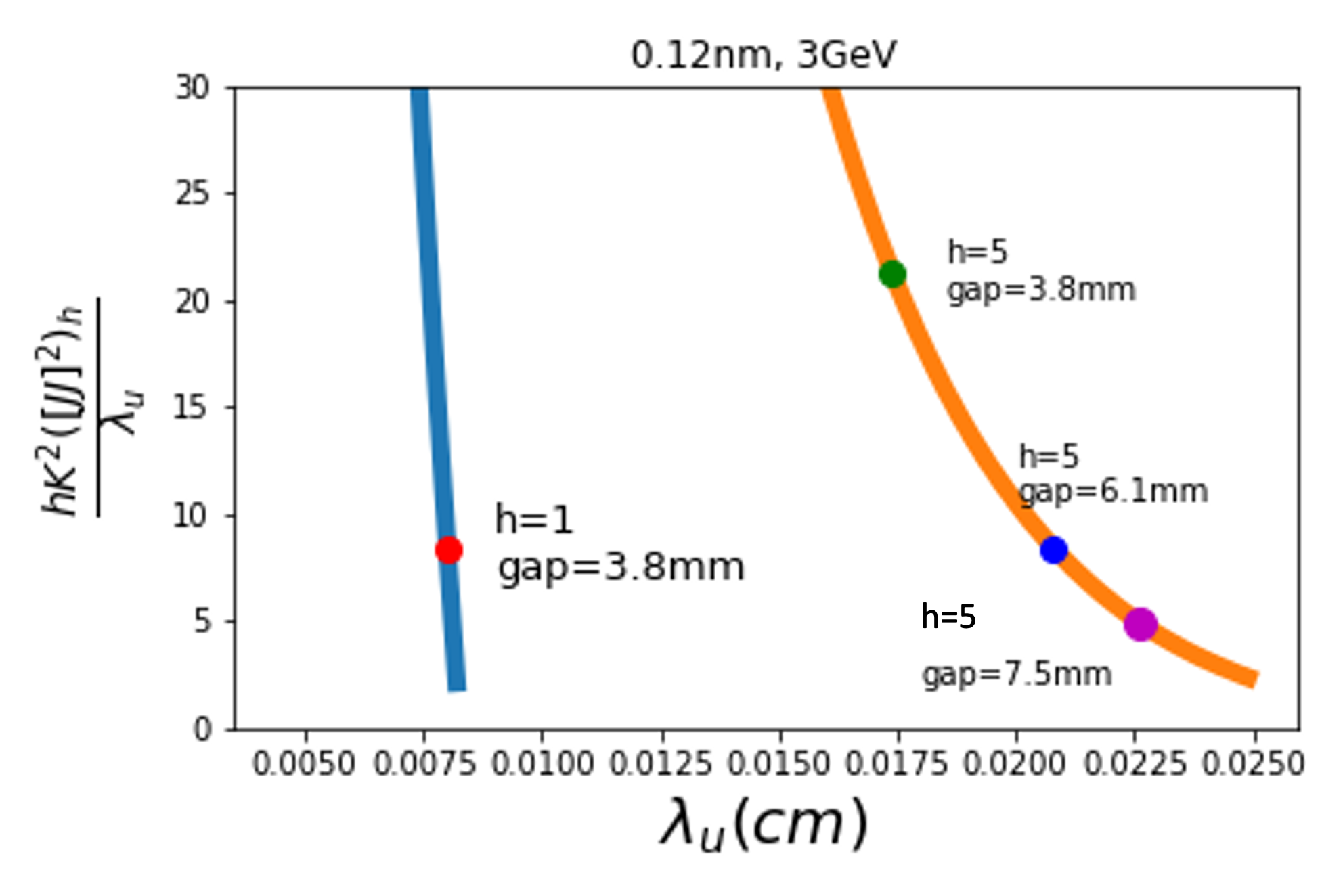
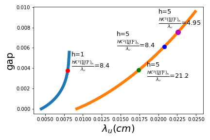
Figure 1: a: $\frac{K^{2}[JJ]_{n}^{2}h}{\lambda_{u}}$ vs. $\lambda_{u}$, compare h=5 with h=1   b: gap vs. $\lambda_{u}$,

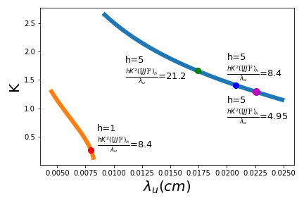
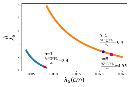
Figure 2: a:   K vs. $\lambda_{u}$,   b: $\frac{h}{\lambda_{u}}$ vs. $\lambda_{u}$,

However, the contribution from the 3rd factor $\frac{d}{d\Phi}\left(\frac{\text{sin}\Phi}{\Phi}\right)^{2}$ is more complicated, with a maximum of 0.54 at $\Phi=-1.3$, the term $2\eta h\pi N_{u}=2\eta\pi L_{u}\frac{h}{\lambda_{u}}$ in $\Phi$ has a spread proportional to $h/\lambda_{u}$ due to the energy spread $\sigma_{\eta}$, the increased spread would reduce the average value of the 3rd factor. To see its effect on the spread of $\Phi$, we plot $h/\lambda_{u}$ as a function of $\lambda_{u}$in Fig.2b. For the pair of points in Fig.1a with the same first gain factor 8.4, we see the ratio $\frac{h}{\lambda_{u}}$ increases from 1.2 for $h=1$ to 2.6 for $h=5$. This reduction is significant, hence the main question in the following discussion is whether the gain reduction due to the large energy spread can be mitigated by TGU and dispersion sufficiently to maintain the required gain.

In the formulation developed in (lindberg, ; ysLi, ; kim4, ) about the 3D gain, if we assume the gradient is in the vertical direction, then the undulator parameter $K=K_{0}(1+\alpha y)$, the energy is $\gamma=\gamma_{0}(1+\eta)$, for $\alpha y\ll 1,\eta\ll 1$, the resonance condition becomes

$$\lambda=\frac{\lambda_{u}}{2\gamma^{2}h}(1+\frac{K^{2}}{2})$$ (4)

$$=\frac{\lambda_{u}}{2\gamma_{0}^{2}h}\frac{1+\frac{K_{0}^{2}}{2}(1+\alpha y)^{2}}{(1+\eta)^{2}}\approx\frac{\lambda_{u}}{2\gamma_{0}^{2}h}\left(1+\frac{K_{0}^{2}}{2}\right)\left(1+\frac{2K_{0}^{2}}{2+K_{0}^{2}}\alpha y-2\eta\right)$$

If we assume the dispersion is $D$ in vertical direction, the vertical distritbution is in gaussian form $\exp(-\frac{(y-D\eta)^{2}}{2\sigma_{y}^{2}})$. the centroid of the electron beam with energy $\eta$ is shifted to $D\eta$, then for very small $\sigma_{y}$, we can take $y\approx D\eta$, and the deviation from resonance condition due to the spread in $\eta$ is given by $\frac{2K_{0}^{2}}{2+K_{0}^{2}}\alpha D\eta-2\eta$. If $\alpha D=\frac{2+K_{0}^{2}}{K_{0}^{2}}$, then the gain reduction due to large energy spread is mitigated. However, there is a trade off with increased verital beam size. The term $\frac{2K_{0}^{2}}{2+K_{0}^{2}}\alpha\sigma_{y}$ causes a deviation from resonance condition in Eq.(4) and $D\sigma_{y}$ increases the transverse beam cross section $\Sigma$ in the gain formula Eq.(1). Both effects reduce the gain, and both are determined by the emittance and focusing in the undulator.

To study the beam quality required for an x-ray FEL working in the medium energy range, we need to apply the gain formula developed in (lindberg, ; ysLi, ; kim4, ) for optimization, with the 3D effect of diffraction, beam divergence, and betatron motion taken into account, and in particular, with addition to include harmonic lasing. In following the procedure to optimize the parameters, we realized that in the formulation in (lindberg, ; ysLi, ; kim4, ), a “no focusing” approximation is taken in the process of derivation of the gain formula using the “brightness function”, as explained clearly after the Eq.(24) of (kim4, ) by K.J. Kim. The “no focusing” approximation essentially neglects the focusing. In our optimization process, we often found that we need to increase the focusing in the undulator, and we reached a set of parameters that violated the condition required by the “no focusing” approximation. Hence it is desirable to develop an approach to calculate the gain without taking the “no focusing” approximation.

In the following we present a derivation of gain formula without taking the “no focusing” approximation, and some examples of the required parameters for a medium energy storage ring such as NSLSII. In Section II, we first follow (kim4, ) to describe the general 3D gain formula resemble 1-D Madey theorem, the Eq.(23) in (kim4, ). This general gain formula, without being given a specific gaussian form of the electron beam distribution and the input radiation field, is our starting point, which is also the last step in (lindberg, ; ysLi, ; kim4, ) right before taking the “no focusing” approximation. Then in Section III, we consider a focusing lattice interlaced with the undulator, the system has nearly constant beta and dispersion functions and hence has nearly constant transverse beam profile in the undulator, this allows us to carry out a multivariable gaussian integration without taking the “no focusing” approximation and reduce the gain formula to a double integral, similar to the result of (lindberg, ; ysLi, ; kim4, ). In Section IV we present some examples of gain optimization using the formula to study the required paramters for an X-ray FEL oscillator in a medium energy storage ring such as the upgrade being considered at the NSLSLII. In Section V, we carry out gain optimization with collective effects taken into account.The resut indicates the feasibility of XFELO for a 3GeV storage ring at NSLSII. In the Appendix I, in order to clarify the notations in this paper and in particular to include the harmonic number $h$ in the formulation, we briefly describe the steps that lead to the general 3D gain formula in Section I, starting from the combined Maxwell-Vlasov equations.

II Gain Formula

The gain in small signal, low gain regime taking into account of the 3D effect of diffracrion, beam divergence and betatron motion, is given in the following Eq.(5 ), which is the Eq.(23) of (kim4, ), with a minor elaboration of introducing the transverse gradient and dispersion for TGU as in (lindberg, ; ysLi, ). For convenience we adopt nearly identical notation as (kim4, ), with only few exceptions to unite with the notations in (lindberg, ; ysLi, ; kim4, ) and the notations we used in the early development of the coupled Maxwell-Vlasov equations for high gain FEL(wang, ; prA, ; PRL, ; HGHG, ). The gain expression has multiple integrations to be carried out for application:

$$G=-c_{h}\frac{\int d\eta d\mathbf{\bm{x}}d\mathbf{\bm{p}}\overline{F}(\mathbf{\bm{x}},\mathbf{\bm{p}},\eta;0)\frac{\partial}{\partial\eta}\mid\int d\bm{\phi}A_{\nu}^{(0)}(\bm{\phi},0)U_{\nu}^{*}(\eta,\bm{\phi},\mathbf{\bm{p}},\mathbf{\bm{x}})\mid^{2}}{\int\mid A^{(0)}(\bm{\phi})\mid^{2}d\bm{\phi}}$$ (5)

where $\mathbf{x}=(x,y)$, $\mathbf{p}=(p_{x},p_{y})$ , $\bm{\phi}=(\phi_{x},\phi_{y})$. $\overline{F}$ is the averaged smooth electron beam background distribution, we assume

$$\overline{F}(\mathbf{\bm{x}},\mathbf{\bm{p}},\eta;z)=\frac{e^{-\eta^{2}/(2\sigma_{\eta}^{2})}}{(2\pi)^{3/2}\sigma_{px}\sigma_{py}\sigma_{\eta}}\exp(-\frac{x^{2}}{2\sigma_{x}^{2}}-\frac{(y-D\eta)^{2}}{2\sigma_{y}^{2}})\exp(-\frac{p_{x}^{2}}{2\sigma_{px}^{2}}-\frac{p_{y}^{2}}{2\sigma_{py}^{2}})$$ (6)

So the electron beam density is $n_{0}\int d\eta dp_{x}dp_{y}\overline{F}(x,p,\eta;z)$, independent of $z$. $n_{0}$ is normalized such that when $D=0$, i.e., before entering into the dispersion region, the peak density at $x=y=0$ is $n_{0}$, so $\int d\eta dp_{x}dp_{y}\overline{F}(0,0,p_{x},p_{y},,\eta;0)\mid_{D=0}=1$. We assume approximately the electron beam in the undulator is matched with constant betatron function such that $\sigma_{px}=k_{\beta x}\sigma_{x}=\sigma_{x}/\beta_{x}$, $\sigma_{py}=k_{\beta y}\sigma_{y}=\sigma_{y}/\beta_{y}$, $p_{x}=\frac{dx}{dz}$,$p_{y}=\frac{dy}{dz}$.

$A_{\nu}(\phi_{x},\phi_{y},z)$ is the angular representation of Fourier transform $a_{\nu}$ of the horizontal electric field component $E$ at frequency $\omega=\nu\omega_{1}$, while the resonance harmonic frequency is $\omega_{s}=h\omega_{1}$in Eq.(2), where $\omega_{1}=2\pi/\lambda_{1}$ is the fundamental frequency.

$$E(x,y,z,t)=\frac{1}{\sqrt{2\pi}}\int e^{-i\Delta\nu k_{u}z}e^{-i\nu\left(k_{1}z-\omega_{1}t\right)}a_{\nu}(x,y,z)\omega_{1}d\nu$$ (7)

$$A_{\nu}(\phi_{x},\phi_{y};z)=\frac{1}{\lambda^{2}}\intop d\mathbf{x}a_{\nu}(\mathbf{x},z)e^{ik\left(x\phi_{x}+y\phi_{y}\right)}$$

where $\omega=2\pi/\lambda,k_{u}=2\pi/\lambda_{u},k_{1}=\omega_{1}/c,k=\omega/c=\nu\omega_{1}/c=\nu k_{1}$, the detuning is given by $\left(\omega-\omega_{s}\right)/\omega_{s}=(\nu-h)/h=\Delta\nu/h$.

We assume the input radiation $a_{\nu}^{(0)}(x,y,z)$, the solution of the Maxwell equation in free space, is a gaussian beam with frequency $\nu$ and Rayleigh range $z_{Rx}=\frac{\pi w_{x}^{2}}{\lambda},z_{Ry}=\frac{\pi w_{x}^{2}}{\lambda}$, where $w_{x}=2\sigma_{rx}$,$w_{y}=2\sigma_{ry}$. $\sigma_{rx},\sigma_{ry}$ are the RMS input laser beam size. Since in the gain formula Eq.(5) the factor $A_{\nu}^{(0)}A_{\nu}^{*(0)}$ appears in both the numerator and the denominator, to simplify writing, we shall take the constant coefficients as $1$ in $a_{\nu}^{(0)}(x,y,z)$ without changing the gain $G$.

$$E(x,z)\sim a_{\nu}^{(0)}(x,y,z)\exp(-ikz)=\frac{1}{\sqrt{q_{x}(z)}}\frac{1}{\sqrt{q_{y}(z)}}\exp(-ik\frac{x^{2}}{2q_{x}(z)}-ik\frac{y^{2}}{2q_{y}(z)}-ikz)$$

$$q_{x}(z)=z+iz_{Rx},q_{y}(z)=z+iz_{Ry}$$

Then Eq.(7) gives the angular representation of input radiation $A_{\nu}^{(0)}(\phi_{x},\phi_{y},0)$ in Eq.(5):

$$A_{\nu}^{(0)}(\phi_{x},\phi_{y},z)=\frac{1}{\sqrt{\lambda}}\exp(ik(z+iz_{Rx})\frac{\phi_{x}{}^{2}}{2})\frac{1}{\sqrt{\lambda}}\exp(ik(z+iz_{Ry})\frac{\phi_{y}{}^{2}}{2})=A_{\nu}^{(0)}(\phi_{x},\phi_{y},0)\exp(ikz\frac{\phi_{x}{}^{2}+\phi_{y}{}^{2}}{2})$$ (8)

$$\text{with }A_{\nu}^{(0)}(\phi_{x},\phi_{y},0)=\frac{1}{\lambda}\exp(-kz_{Rx}\frac{\phi_{x}{}^{2}}{2}-kz_{Ry}\frac{\phi_{y}{}^{2}}{2})$$

Thus the angular divergence RMS value is $\sigma_{\phi x}=\sigma_{rx}/z_{Rx},\sigma_{\phi y}=\sigma_{ry}/z_{Ry}$ .

The undulator radiation amplitude in Eq.(5) is $U_{\nu}^{*}(\eta,\phi_{x},\phi_{y},p_{x},y)$

$$U_{\nu}^{*}(\bm{\phi},\eta,\mathbf{x},\mathbf{p};z)=\intop_{-L/2}^{L/2}dse^{-ik\mathbf{x}\bm{\phi}}e^{i\intop_{0}^{s}ds_{1}\xi_{\nu}(\bm{\phi},\eta,\mathbf{x},\mathbf{p};s_{1})}$$

$$\text{where }\xi_{\nu}(\phi,\eta,\mathbf{x},\mathbf{p};s)=((\Delta\nu-2\nu\eta)k_{u}+\nu\frac{2K_{0}^{2}}{2+K_{0}^{2}}\alpha k_{u}y_{0}+\frac{k}{2}((p_{0x}-\phi_{x})^{2}+k_{\beta x}^{2}x_{0}^{2}+(p_{0y}-\phi_{y})^{2}+k_{\beta y}^{2}y_{0}^{2})$$ (9)

where $\mathbf{x}_{0}(s;\mathbf{x},\mathbf{p})$,$\mathbf{p}_{0}(s;\mathbf{x},\mathbf{p})$ are solutions of the equations of betatron motion

$$\frac{dx}{ds}=p_{x},\frac{dy}{ds}=p_{y}$$

$$\frac{dp_{x}}{ds}=-k_{\beta x}^{2}x^{2},\frac{dp_{y}}{ds}=-k_{\beta y}^{2}y^{2}$$ (10)

with the initial condition $\mathbf{x}_{0}(s=0;\mathbf{x},\mathbf{p})=\mathbf{x}$,$\mathbf{p}_{0}(s=0;\mathbf{x},\mathbf{p})=\mathbf{p}$. Here we neglect the focusing introduced by the gradient $\alpha$, and we assumed the focusing comes from the natural focusing and the external focusing of a FODO lattice, and approximate the beta function by constants.

The constant $c_{h}=\frac{e^{2}K^{2}[JJ]_{h}^{2}n_{0}}{8mc^{2}\epsilon_{0}\gamma^{3}\lambda^{2}}$, where the electron beam density at the peak is determined by current $I=ecn_{0}\Sigma=2\pi\sigma_{x}\sigma_{y}ecn_{0}$ (the current of an approximately flat top bunch with transverse gaussian distribution). To write the gain $G$ into a form convenient for scaling with $h$ and $\lambda_{u}$, as shown in Eq.(1), we have (with Alven current $I_{A}=4\pi mc^{3}\epsilon_{0}/e)$

$$c_{h}=\frac{I}{I_{A}}\frac{\pi K^{2}[JJ]_{h}^{2}}{\gamma^{3}}\frac{1}{4\pi\sigma_{x}\sigma_{y}\lambda^{2}}$$ (11)

To calculate the gain $G$ we need to carry out the multivariable integral in Eq.(5). Before the multivariable integration, the approach in(lindberg, ; ysLi, ) is to first take a “no focusing approximation” by neglecting the terms $k_{\beta x}^{2}x_{0}^{2}+k_{\beta y}^{2}y_{0}^{2}$, following the step prescribed in (kim4, ). With this approximation, a gain formula can be transformed into a form where the integrand becomes a convolution of the distribution function with the radiation brightness and undulator brightness. This form is appropriate for a gaussian integration which finally leads to a double integral convenient for numerical calculation.

The condition for neglecting $k_{\beta x}^{2}x_{0}^{2}$ in $(p_{0x}-\phi_{x})^{2}+k_{\beta x}^{2}x_{0}^{2}$, because $p_{x}$ and $k_{\beta x}x$ are about the order of $k_{\beta x}\sigma_{x}$, corresponds to require $\sigma_{\phi x}\gg k_{\beta x}\sigma_{x}$. Same way it requires $\sigma_{\phi y}\gg k_{\beta y}\sigma_{y}$. We found often our optimization leads to a set of parameters that violate this condition, in particular, when emittance is not very small and we need to increase $k_{\beta}$. In fact, in the example we developed in Section IV, for $\epsilon_{x0}=80pm,$the optimized $\beta_{x}=6.6m$ and Rayleigh range $Z_{Rx}=4m$ gives $k_{\beta}\sigma_{x}/\sigma_{\phi x}\approx 2.3$.

Hence we would like to try to take into account the effect of the betatron motion in the gain optimization without the limitation imposed by this condition. To maintain approximately constant beta and dispersion functions along the full length of the undulator, we considered a FODO lattice of focusing interlaced with the sections of the undulator, with dipole correctors next to the quadrupoles of the FODO lattice to keep an almost straight line for an approximately constant dispersion in the transverse gradient undulator. When the beta functions and dispersion are kept approximately constant, the beam transverse profile is approximately invariant along the undulator, the interaction between the effects of the betatron motion, the dispersion, and the FEL embodied in the integral in Eq.(5) is significantly simplified. Under this circumstance, it turns out without neglecting the focusing, the multiple integral are still possible to be reduced to a double integral, mainly because the integrations over $x,p_{x},y,p_{y},\eta,\phi_{x},\phi_{y}$ are all gaussian, as given in Section III.

III Gain Calculation by gaussian integration

To write the integrand in Eq.(5) into a gaussian integral, we first separate the variable $\bm{\phi}$ in Eq.(9)

$$\xi_{\nu}(\phi,\eta,\mathbf{x},\mathbf{p};s)=\xi_{\nu}^{(0)}(\eta,x,p;s)-k\mathbf{p}_{0}(s)\bm{\phi}+\frac{k}{2}\bm{\phi}^{2}$$

$$\text{where }\xi_{\nu}^{(0)}(\eta,x,p;s)\equiv\xi_{\nu}(\phi=0,\eta,\mathbf{x},\mathbf{p};s_{1})=(\Delta\nu-2\nu\eta)k_{u}+\nu\frac{2K_{0}^{2}}{2+K_{0}^{2}}\alpha k_{u}y_{0}+\frac{k}{2}(p_{x}^{2}+k_{\beta x}^{2}x^{2}+p_{y}^{2}+k_{\beta y}^{2}y^{2})$$ (12)

Because the last term in $\xi_{\nu}^{(0)}$ is invariant independent of $s$, $\mathbf{x}_{0}$,$\mathbf{p}_{0}$ are replaced by the initial value $\mathbf{x},\mathbf{p}$, and the only term dependent on $s$ is $4\nu\zeta_{0}\alpha k_{u}y_{0}(s)$. Since $\mathbf{x}+\intop_{0}^{s}ds_{1}\mathbf{p}_{0}(s)\bm{\phi}=\mathbf{x_{0}}(s)$, we have $U_{\nu}^{*}(\bm{\phi},\eta,\mathbf{x},\mathbf{p};z)=\intop_{-L/2}^{L/2}dse^{-ik\mathbf{x_{0}}(s)\bm{\phi}+i\frac{k}{2}\bm{\phi}{}^{2}s}e^{i\intop_{0}^{s}ds_{1}\xi_{\nu}^{(0)}(\eta,\mathbf{x},\mathbf{p};s_{1})}$ in Eq.(9). So the gain in Eq.(5) is

$$G=-c_{h}I_{1e}\left(\int\mid A^{(0)}(\bm{\phi})\mid^{2}d\bm{\phi}\right)^{-1}$$

$$\text{where }I_{1e}\equiv\int\int\int d\eta d\mathbf{x}d\mathbf{p}\overline{F}(\mathbf{x},\mathbf{p},\eta;0)\frac{\partial}{\partial\eta}\mid\intop_{-L/2}^{L/2}dsI_{1r}e^{i\intop_{0}^{s}ds_{1}\xi_{\nu}^{(0)}(\eta,\mathbf{x},\mathbf{p};s_{1})}\mid^{2}$$ (13)

$$\text{with }I_{1r}(s)\equiv\int d\bm{\phi}A^{(0)}(\bm{\phi})e^{-ik\mathbf{x_{0}}(s)\bm{\phi}+i\frac{k}{2}\bm{\phi}{}^{2}s}$$

substitute Eq.(8) into $I_{1r}(s)$ and use $x_{0}(s)=x\cos(\frac{s}{\beta_{x}})+\beta_{x}p_{x}\sin(\frac{s}{\beta_{x}}),y_{0}(s)=y\cos(\frac{s}{\beta_{y}})+\beta_{y}p_{y}\sin(\frac{s}{\beta_{y}})$, we find

$$I_{1r}(s)=-i\frac{1}{\sqrt{z_{Rx}-is}\sqrt{z_{Ry}-is}}\exp(c_{x}(s)x^{2}+2c_{xp}(s)xp_{x}+c_{px}(s)p_{x}^{2})\exp(c_{y}(s)y^{2}+2c_{yp}(s)yp_{y}+c_{py}(s)p_{y}^{2})$$

$$\text{where }c_{x}(s)\equiv-k\frac{\cos^{2}(\frac{s}{\beta_{x}})}{2(z_{Rx}-is)},c_{px}(s)\equiv-k\frac{\beta_{x}^{2}\sin^{2}(\frac{s}{\beta_{x}})}{2(z_{Rx}-is)},c_{xp}(s)\equiv-k\frac{\beta_{x}\cos(\frac{s}{\beta_{x}})\sin(\frac{s}{\beta_{x}})}{2(z_{Rx}-is)}$$ (14)

$$c_{y}(s)\equiv-k\frac{\cos^{2}(\frac{s}{\beta_{y}})}{2(z_{Ry}-is)},c_{py}(s)\equiv-k\frac{\beta_{y}^{2}\sin^{2}(\frac{s}{\beta_{y}})}{2(z_{Ry}-is)},c_{yp}(s)\equiv-k\frac{\beta_{y}\cos(\frac{s}{\beta_{y}})\sin(\frac{s}{\beta_{y}})}{2(z_{Ry}-is)}$$

$$\left(\int\mid A^{(0)}(\bm{\phi})\mid^{2}d\bm{\phi}\right)^{-1}=2\pi\text{$w_{x}w_{y}$}$$

$$I_{1e}=\int\int\int d\eta d\mathbf{x}d\mathbf{p}\overline{F}(\mathbf{x},\mathbf{p},\eta;0)\frac{\partial}{\partial\eta}\intop_{-L/2}^{L/2}\intop_{-L/2}^{L/2}dsdz\mid I_{1r}(s)I_{1r}^{*}(z)\mid e^{i\intop_{0}^{s}ds_{1}\xi_{\nu}^{(0)}(\eta,x,p;s_{1})}e^{-i\intop_{0}^{z}ds_{1}\xi_{\nu}^{(0)}(\eta,x,p;s_{1})}$$

Substitute $\intop_{0}^{s}ds_{1}y_{0}(s)$ into Eq.(12), we get

$$\intop_{0}^{s}ds_{1}\xi_{\nu}^{(0)}(\eta,x,p;s_{1})=(\Delta\nu-2\nu\eta)k_{u}s+\frac{k}{2}(p_{x}^{2}+k_{\beta x}^{2}x^{2}+p_{y}^{2}+k_{\beta y}^{2}y^{2})s$$

$$+\nu\frac{2K_{0}^{2}}{2+K_{0}^{2}}\alpha k_{u}\beta_{y}y\left(\sin(\frac{s}{\beta_{y}})-\sin(\frac{z}{\beta_{y}})\right)-\nu\frac{2K_{0}^{2}}{2+K_{0}^{2}}\alpha k_{u}\beta_{y}^{2}p_{y}\left(\cos(\frac{s}{\beta_{y}})-\cos(\frac{z}{\beta_{y}})\right)$$ (15)

With$\text{ }\frac{\partial}{\partial\eta}i\intop_{0}^{s}ds_{1}\xi_{\nu}^{(0)}(\eta,x,p,s_{1})-\frac{\partial}{\partial\eta}i\intop_{0}^{z}ds_{1}\xi_{\nu}^{(0)}(\eta,x,p,s_{1})=-2i\nu k_{u}(s-z)$, we have

$$I_{1e}=\intop_{-L/2}^{L/2}\intop_{-L/2}^{L/2}dsdz\int\int\int d\eta d\mathbf{x}d\mathbf{p}I_{1r}(s)I_{1r}^{*}(z)\overline{F}(\mathbf{x},\mathbf{p},\eta;0)e^{i\intop_{0}^{s}ds_{1}\xi_{\nu}^{(0)}(\eta,x,p;s_{1})}e^{-i\intop_{0}^{z}ds_{1}\xi_{\nu}^{(0)}(\eta,x,p;s_{1})}(-2i\nu k_{u})(s-z)$$

Collect all the exponential factors in $I_{1r}(s)I_{1r}^{*}(z)$ $\overline{F}(x,p,\eta;0)$ and in $e^{i\intop_{0}^{s}ds_{1}\xi_{\nu}^{(0)}(\eta,x,p;s_{1})},e^{-i\intop_{0}^{z}ds_{1}\xi_{\nu}^{(0)}(\eta,x,p;s_{1})}$ together (See Eq.(14), and Eq.(6), and Eq.(15)) and let

$$D_{R}(s,z)\equiv\sqrt{z_{Rx}-is}\sqrt{z_{Ry}-is}\sqrt{z_{Rx}+iz}\sqrt{z_{Ry}+iz}$$ (16)

we find

$$I_{1e}=\intop_{-L/2}^{L/2}\intop_{-L/2}^{L/2}dsdz\left(\frac{(-i2\nu k_{u})(s-z)}{D_{R}(s,z)}\frac{\exp(i\Delta\nu k_{u}(s-z))}{(2\pi)^{3/2}\sigma_{px}\sigma_{py}\sigma_{\eta}}\right)I_{x}(s,z)I_{y\eta}(s,z)$$ (17)

$$\text{where }I_{x}(s,z)=\int\int dxdp_{x}\exp(-\Phi_{x})$$

$$I_{y\eta}(s,z)=\int\int d\eta dydp_{y}\exp(-\Phi_{y\eta})$$

with

$$\Phi_{x}=A_{x}x^{2}+A_{px}p_{x}^{2}+B_{xp}xp_{x}$$

$$A_{x}=\frac{1}{2\sigma_{x}^{2}}D_{x},D_{x}=1-2\sigma_{x}^{2}\left[c_{x}(s)+c_{x}^{*}(z)\right]-ikk_{\beta x}^{2}\sigma_{x}^{2}(s-z)$$ (18)

$$A_{px}=\frac{1}{2\sigma_{px}^{2}}D_{px},D_{px}=1-2\sigma_{px}^{2}\left[c_{px}(s)+c_{px}^{*}(z)\right]-ik\sigma_{px}^{2}(s-z)$$

$$B_{xp}=-2\left[c_{xp}(s)+c_{xp}^{*}(z)\right]$$

and

$$\Phi_{y\eta}=A_{\eta}\eta^{2}+A_{y}y^{2}+A_{py}p_{y}^{2}+B_{\eta y}y\eta+B_{yp}y\eta+B_{\eta}\eta+B_{y}y+B_{py}p_{y}$$

$$A_{\eta}\equiv\frac{1}{2\sigma_{\eta}^{2}}+\frac{D^{2}}{2\sigma_{y}^{2}},A_{py}\equiv\frac{1}{2\sigma_{py}^{2}}D_{py},D_{py}=1-2\sigma_{py}^{2}\left[c_{py}(s)+c_{py}^{*}(z)\right]-ik\sigma_{py}^{2}(s-z)$$ (19)

$$A_{y}\equiv\frac{1}{2\sigma_{y}^{2}}-\left[c_{y}(s)+c_{y}^{*}(z)\right]-i\frac{k}{2}k_{\beta y}^{2}(s-z)$$

$$B_{\eta y}=-\frac{D}{\sigma_{y}^{2}},B_{yp}=-2\left[c_{yp}(s)+c_{yp}^{*}(z)\right],B_{\eta}=2i\nu k_{u}(s-z)$$

$$B_{y}=-B_{\alpha}c_{s}(s,z),B_{py}=B_{\alpha}\beta_{y}c_{c}(s,z),B_{\alpha}\equiv i\nu\frac{2K_{0}^{2}}{2+K_{0}^{2}}\alpha k_{u}\beta_{y}$$

$$\text{where }c_{s}(s,z)\equiv\left(\sin(\frac{s}{\beta_{y}})-\sin(\frac{z}{\beta_{y}})\right),c_{c}(s,z)\equiv\left(\cos(\frac{s}{\beta_{y}})-\cos(\frac{z}{\beta_{y}})\right)$$ (20)

$\Phi_{x}$ and $\Phi_{y\eta}$ are quadratic polynomials in $x,p_{x}$ and in $\eta,y,p_{y}$respectively. Their coefficients are functions of $s,z$ only. By linear transformation, they can be transformed into diagonal quadratic form. Hence $I_{x}(s,z),I_{y\eta}(s,z)$ are gaussian integrals. In Appendix II we give a brief description of the process of transforming to gaussian integration. The result is

$$I_{x}=\frac{2\pi\sigma_{px}\sigma_{x}}{\sqrt{(D_{x}D_{px}-\sigma_{x}^{2}\sigma_{px}^{2}B_{xp}^{2})}}$$ (21)

$$I_{y\eta}=\frac{\left(2\pi\right)^{\frac{3}{2}}}{\sqrt{D_{py}}}\frac{\sigma_{\eta}\sigma_{y}\sigma_{py}}{\sqrt{D_{\eta y}}}\exp\left(\frac{N_{\eta y}}{D_{\eta y}}\sigma_{\eta}^{2}\sigma_{y}^{2}\right)$$

where $D_{x},D_{px},D_{py},B_{xp}$ are given in Eq.(18,19) and

$$D_{\eta y}=1+\left(\sigma_{y}^{2}+D^{2}\sigma_{\eta}^{2}\right)\left(2A_{y}-\frac{1}{\sigma_{y}^{2}}-\frac{\sigma_{py}^{2}B_{yp}^{2}}{D_{py}}\right)$$

$$N_{\eta y}=C_{ss}c_{s}^{2}(s,z)+C_{0}+C_{s}c_{s}(s,z)+C_{sc}c_{s}(s,z)c_{c}(s,z)+C_{cc}c_{c}^{2}(s,z)+C_{c}c_{c}(s,z)$$ (22)

The sinusoidal functions $c_{s}(s,z)$,$c_{c}(s,z)$ are given by Eq.(19). Their coefficients in $N_{\eta y}(s,z)$ are also functions of $s,z$:

$$C_{ss}=B_{\alpha}^{2}A_{\eta},C_{0}=B_{\eta}^{2}\left(A_{y}-\frac{B_{yp}^{2}}{4A_{py}}\right),C_{s}=B_{\eta}B_{\alpha}B_{\eta y}$$

$$C_{sc}=\frac{B_{yp}B_{\alpha}^{2}\beta_{y}A_{\eta}}{A_{py}},C_{cc}=\frac{B_{\alpha}^{2}\beta_{y}^{2}}{A_{py}}\left(A_{\eta}A_{y}-\frac{1}{4}B_{\eta y}^{2}\right),C_{c}=\frac{B_{\eta}B_{\alpha}B_{\eta y}B_{yp}\beta_{y}}{2A_{py}}$$ (23)

With these provisions, we find the gain $G$ as a double integral over $s,z$. First substitute Eq.(22) into Eq.(17) to find $I_{1e}$, then substitute $I_{1e}$, $\left(\int\mid A^{(0)}(\bm{\phi})\mid^{2}d\bm{\phi}\right)^{-1}$from Eq.(14), and the constant$c_{h}$ in Eq.(11) into Eq.(13), with $\nu\approx h$, we finally have

$$G=-\left(\frac{hK^{2}[JJ]_{h}^{2}}{\lambda_{u}}\right)\left(\frac{I}{I_{A}}\frac{\pi^{2}}{\gamma^{3}}\right)\left(2I_{3D}\right)\frac{\text{$2\pi w_{x}w_{y}$}}{\lambda^{2}},$$

$$\text{with }I_{3D}=\intop_{-L/2}^{L/2}\intop_{-L/2}^{L/2}dsdz\frac{-i(s-z)\exp(i\Delta\nu k_{u}(s-z))}{\sqrt{(D_{x}D_{px}-\sigma_{x}^{2}\sigma_{px}^{2}B_{xp}^{2})}\sqrt{D_{py}}\sqrt{D_{\eta y}}}\exp\left(\frac{N_{\eta y}}{D_{\eta y}}\sigma_{\eta}^{2}\sigma_{y}^{2}\right)\frac{1}{D_{R}(s,z)}$$ (24)

where $D_{\eta y},N_{\eta y}$ are given by Eqs.(22,23). The coefficients in $D_{\eta y},N_{\eta y}$ are expressed by the coefficients $A_{\eta},A_{y},A_{py}$ ,$B_{\eta},B_{\alpha},B_{\eta y},B_{yp},B_{xp}$and $D_{x},D_{px},D_{py}$ of the polynomial $\Phi_{x},\Phi_{y\eta}$ in the gaussion integral, as given by Eq.(18,19). The expressions in these coefficients, $c_{x}(s),c_{xp}(s),c_{px}(s),c_{y}(s),c_{yp}(s),c_{py}(s)$, are given in Eq.(14). The sinusoldal functions $c_{s}(s,z),c_{c}(s,z)$ in $N_{\eta y}$ are given in Eq.(19).

Because of effect of the betatron motion, the structure of the factors in $I_{3D}$ is more complicated than the corresponding double integral in (lindberg, ; ysLi, ). However, the numerical calculation of the double integral is simple, so it is appropriate for optimization.

As a check, in 1D limit, $D_{x}=D_{px}=D_{py}=D_{\eta y}=1$,$B_{xp}=0$,$D_{R}(s,z)=z_{Rx}z_{Ry}=\frac{\pi^{2}w_{x}^{2}w_{y}^{2}}{\lambda^{2}}$. The radiation beam size is the same as the electron beam size $\sigma_{rx}=w_{x}/2=\sigma_{x}$,$\sigma_{ry}=w_{y}/2=\sigma_{y}$ . If energy spread is negligible, $\sigma_{\eta}=0$, we have

$$I_{3D}=\left(\intop_{-L/2}^{L/2}\intop_{-L/2}^{L/2}dsdz\left(-i(s-z)\exp(i\Delta\nu k_{u}(s-z))\right)\right)\frac{\lambda^{2}}{\pi^{2}w_{x}^{2}w_{y}^{2}}$$

$$=-L^{3}\frac{1}{2}\frac{d}{dx}\left(\frac{\sin\Phi}{\Phi}\right)_{\Phi=\Delta\nu k_{u}L/2}^{2}\left(\frac{\lambda^{2}}{\pi^{2}w_{x}^{2}w_{y}^{2}}\right)$$

Then $G$ becomes the $G_{1D}$ given by Eq.(1).

IV An Example of Gain Calculation

The Eq.(24) is the main result of this paper. Our goal is to apply this formula to explore the possibility of a hard x-ray FEL for a light source at energy as low as 3GeV, and in particular, to find the required electron beam quality and undulator for an upgrade of NSLSII to drive a hard x-ray FEL to help to study if it is possible.

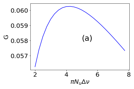
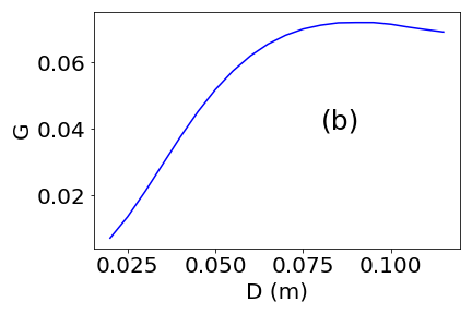
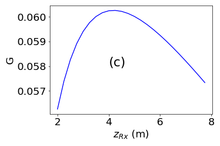
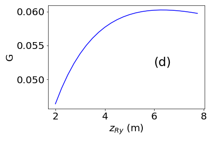
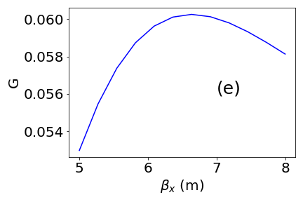
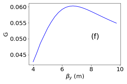
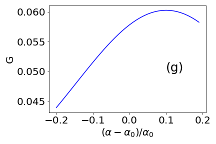
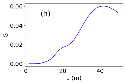
Figure 3: G vs. (a)$\Delta\nu$,   (b)D,   (c)$z_{Rx}$ ,  (d)$z_{Rx}$,   (e)$\beta_{x}$,   (f)$\beta_{y}$,    (g)($\alpha-\alpha_{0})/\alpha_{0}$,   (h) L

E (GeV)	I (A)	$\lambda_{u}$(cm)	h	G(%)	$K_{0}$	$\epsilon_{x}$ (pm)	$\epsilon_{y}$ (pm)	D (m)	$\beta_{x}$(m)	$\beta_{y}$(m)	$z_{Rx}$(m)	$z_{Ry}$(m)	$\alpha$ ($m^{-1})$	$\sigma_{x}$($\mu m)$	$\sigma_{y}$($\mu m)$
3	73	2.26	5	6.0	1.29	80	1.7	0.05(V)	6.6	6.9	4.0	6.3	49	23	3.5

Table 1: Parameters for maximum $G$

First, taking collective effects into account, we assume a 3GeV FEL at 0.12nm, approximate the bunch as a flat top pulse, the current $I=73A$ for a bunch length 180ps. For this example, we assume a local coupling correction in the undulator section to minimize the local vertical emittance and to blow up the vertical emittance in the rest of the ring for mitigation of the intra-beam scattering. The revolution period is about 2.6$\mu s$, so the bunch current is 5mA. As discussed in the Section I, we plot the first factor $\frac{K^{2}[JJ]_{h}^{2}h}{\lambda_{u}}$ in the 1D gain formula as function of $\lambda_{u}$ in Fig.1a, and plot the gap $g$ vs. $\lambda_{u}$ in Fig.1b. For $h=5$, as a compromise between larger gain and gap, we choose $\lambda_{u}=2.26cm$ and $\frac{K^{2}[JJ]_{h}^{2}h}{\lambda_{u}}=4.96m^{-1}$, with gap $g=7.5mm$, $K_{0}=1.29$.

We assume the emittance $\epsilon_{x}=80pm,\epsilon_{y}=1.7\,pm$, energy spread $\sigma_{\eta}=10^{-3}$, and undulator length $L=42m$, and scan the 6 variables: detuning $\Delta\nu$, horizontal dispersion $D$, focusing beta functions $\beta_{x},\beta_{y},$the input radiation Rayleigh ranges $z_{Rx},z_{Ry}$, and the transverse gradient $\alpha$ to find maximum gain. During the scan, we find the transverse gradient $\alpha$ should be allowed to deviate from $\alpha_{0}$ (where $\alpha_{0}D=\frac{2+K_{0}^{2}}{K_{0}^{2}}$). Actually, we find the optimized $\alpha$ close but larger than $\alpha_{0}$.

The plot of scan in the last scan cycle is given in Fig.3. The maximum gain is 7% in the last cycle for dispersion at 8 cm. However we limit the vertical dispersion to 5 cm and the gain is 6.0 %. In the subplot of G vs. L the maximum gain is reached at $L=42m$. The paramters for this setting are given in Table 1. In Table 1 the energy spread is $\sigma_{\eta}=10^{-3}$, the undulator length is taken as $L=42m$, the x-ray wavelength is $\lambda_{s}=0.12nm$, gap $g=7.5mm$. For dispersion $D$, (V) is vertical dispersion.

V. GAIN OPTIMIZATION WITH COLLECTIVE EFFECTS

As one can see in the previous section, XFELO requires quite a high peak beam current and small emittance. The emittance of synchrotron light sources is continuously reduced in past decades. Implementation of the Multi-Bend Achromat (MBA) technology resulted in the development of a new generation of synchrotrons with much lower emittance. Recently, three new MBA-based rings have been commissioned (tavares, ; torino, ; lin, ) and few upgrade projects are being developed worldwide (APS, ; steier, ; jiao, ; Karantzoulis, ; Diamond, ; shin, ). We consider an XFELO option for a lattice based on the recently developed complex bend approach for the future low-emittance upgrade of NSLS-II (Plassard, ). This lattice provides a horizontal emittance of 25 pm at a beam energy of 3 GeV fitting the present NSLS-II tunnel with a circumference of 792 m. We propose to place the 42-m long XFELO undulator in a straight section with a vertical dispersion bypassing three out of 30 achromat cells.

However, collective effects of beam dynamics significantly affect electron beam parameters in medium-energy (3-4 GeV) storage rings because the beams are small in all three dimensions and the particle density in the bunch is quite high. The main adverse effect impeding the achievement of the required combination of beam parameters is intra-beam scattering (IBS). To mitigate the collective effects, higher-harmonic RF cavities are used for bunch lengthening. The other strong intensity-dependent effect is the bunch lengthening due to potential well distortion by the longitudinal impedance of the vacuum chamber.

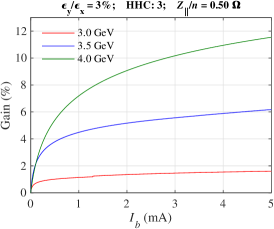
Figure 4: FEL gain optimized taking collective effects into account

For a realistic assessment of a ring-based XFELO, we carried out multi-parameter optimization of the FEL gain Eq.24 assuming the vertical dispersion of 5 cm, emittance, energy spread, and bunch length determined by the lattice model taking into account the effect of IBS together with the impedance-driven bunch lengthening and higher-harmonic cavities. For the low-emittance synchrotrons, the light-generating insertion devices make a major contribution to the total energy loss per turn $U_{0}$ determining the radiation damping, so we include them into the lattice model. We optimized the detuning $\Delta\nu$, beta functions $\beta_{x},\beta_{y}$, the input radiation Rayleigh ranges $z_{Rx},z_{Ry}$, and the transverse gradient $\alpha$ to find the maximum gain.

We applied the high-energy approximation of the IBS theory(bane, ). The equilibrium emittance $\varepsilon_{x,y}$ and relative energy spread $\sigma_{p}$ are expressed as

$$\varepsilon_{x,y}=\frac{\varepsilon_{x0,y0}}{1-\tau_{x,y}/T_{x,y}}\ ,\qquad\sigma_{p}^{2}=\frac{\sigma_{p0}^{2}}{1-\tau_{p}/T_{p}}\ ,$$

where $\varepsilon_{x0,y0}$ and $\sigma_{p0}$ are the emittance and energy spread at zero beam current; $\tau_{x}$, $\tau_{y}$, and $\tau_{p}$ are the radiation damping times; $T_{xy}$, and $T_{p}$ are the IBS growth times:

$$\frac{1}{T_{p}}\simeq\frac{r_{0}^{2}cN}{32\gamma^{3}\varepsilon_{x}\varepsilon_{y}\sigma_{s}\sigma_{p}^{2}}\left(\frac{\varepsilon_{x}\varepsilon_{y}}{\left<\beta_{x}\right>\left<\beta_{y}\right>}\right)^{\!\!1/4}\ln\frac{\left<\sigma_{y}\right>\gamma^{2}\varepsilon_{x}}{r_{0}\left<\beta_{x}\right>}\ ,$$ (25)

$$\frac{1}{T_{x,y}}\simeq\frac{\sigma_{p}^{2}\left<\mathscr{H}_{x,y}\right>}{\varepsilon_{x,y}}\frac{1}{T_{p}}\ ,$$ (26)

$r_{0}$ is classical electron radius, $\sigma_{s}$ is the r.m.s. bunch length, $\sigma_{y}$ is the vertical beam size, $\mathscr{H}_{x,y}$ is the lattice function Eq.27

$$\mathscr{H}=\beta_{x}\eta_{x}^{\prime 2}+2\alpha_{x}\eta_{x}\eta_{x}^{\prime}+\gamma_{x}\eta_{x}^{2}\ ,$$ (27)

$\beta_{x}$ is the amplitude function of betatron oscillation (beta function), $\alpha_{x}\equiv-\beta_{x}^{\prime}/2$, $\gamma_{x}\equiv\frac{1+\alpha_{x}^{2}}{\beta_{x}}$; $\eta_{x}$ and $\eta_{x}^{\prime}$ is the dispersion function and its derivative, respectively. As one can see, the IBS strongly depends on the beam energy, so its effect is not so significant for high-energy rings.

The bunch lengthening caused by the beam interaction with the longitudinal impedance was calculated using the modified Zotter equation(zotter, ) in differential form. The effect of higher-harmonic cavities was simply modeled by a multiplication of the zero-intensity bunch length by a factor of 3.

As a result of the optimization, Fig.4 shows the FEL gain as a function of single-bunch current for the beam energy of 3GeV, 3.5GeV, and 4GeV, and for an extremely low coupling of 3%.

With the constant coupling, the 3-GeV XFELO does not look realistic because the gain is too small but the energy increase results in a feasible gain of 6%, especially for 3.5GeV to 4GeV.

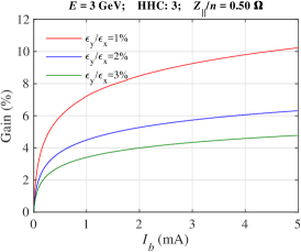
Figure 5: FEL gain optimized with a local coupling correction

However, if we implement a local coupling correction to reduce the vertical beam size only in the undulator section with coupling of 2% while keeping 100% coupling everywhere else in the ring, the XFELO looks feasible with gain reaching 6% even for 3$\sim$GeV energy, see Fig.5.

VI. Summary

We developed a gain formula for a hard x-ray FEL in the medium energy range between 3 and 4.5GeV so that we do not need to take “no focusing approximation” in the calculation, in the hope this can be of use in exploring the possibility of x-ray FEL in this energy range. The formula allows gain calculation with harmonic lasing.

We present an example. The example indicates hard x-ray FEL in 3GeV is feasible, even though it sets rather challenging conditions for the storage ring.

Appendix I Outline of derivation of FEL gain in small signal, low gain regime

The FEL gain is derived from the coupled Maxwell-Vlasov equations, which initially was developed for high gain FEL theory (wang, ; prA, ; PRL, ; HGHG, ). Later it is used for small gain FEL in (lindberg, ; ysLi, ; kim4, ). We outline the gain formula derivation here as given in (kim4, ) in order to clarify the inclusion of the TQU, the dispersion, and we pay attenion to the harmonic number $\nu\approx h$ in this paper. Many of the notations here have been introduced in Section II when we introduce the gain formula. The Maxwell equation in the notation here is

$$\begin{split}(\frac{\partial}{\partial z}-i\Delta\nu k_{u}\end{split}+\frac{i}{2k}\nabla_{\bot}^{2})a_{\nu}(x,z)=-g_{n}\int d\eta\int d\mathbf{p}\delta F_{\nu}(z,\theta,\eta,\mathbf{x},\mathbf{p})$$ (28)

where $g_{n}=\frac{eK[JJ]_{h}n_{0}}{4\epsilon_{0}\gamma\omega_{1}}$, and $n_{0}F(z,\theta,\eta,\mathbf{x},\mathbf{p})=k_{1}\sum\delta(\eta-\eta_{j})\delta(\mathbf{x}-\mathbf{x}_{j})\delta(\mathbf{p}-\mathbf{p}_{j})\delta(\theta-\theta_{j})$ is the electron beam distribution function, $\theta=(k_{1}+k_{u})z-\omega_{1}\overline{t}$ is the micro-bunching phase, $\overline{t}$ is the time of electron passing through $z$ averaged over a period of the undulator. The function $F$ is separated into two parts $F=\overline{F}+\delta F$, $\overline{F}$ is the averaged smooth electron beam background distribution in Eq.(6), $\delta F$ is the deviation from $\overline{F}$ including shot noise in the beam and the micro-bunching due to FEL interaction. $\delta F_{\nu}(z,\theta,\eta,\mathbf{x},\mathbf{p})$ is the Fourier transfrom of $\delta F$:

$$\delta F_{\nu}(\eta,\mathbf{x},\mathbf{p};z)=\frac{1}{\sqrt{2\pi}}\int e^{i\nu\theta}\delta F(z,\theta,\eta,\mathbf{x},\mathbf{p})d\theta$$ (29)

The Vlasov equation is essentially the Liouville theorem applied to perturbation theory in a small signal regime. After Fourier transfrom from $\theta$ to $\nu$, it is in the form

$$\begin{split}(\frac{\partial}{\partial z}\end{split}+\dot{\theta}\frac{\partial}{\partial\theta}+\dot{\mathbf{x}}\frac{\partial}{\partial\mathbf{x}}+\dot{\mathbf{p}}\frac{\partial}{\partial\mathbf{p}})\delta F_{\nu}(\eta,\mathbf{x},\mathbf{p};z)=-h_{h}a_{\nu}(\mathbf{x},z)\frac{\partial}{\partial\eta}\bar{F}(\eta,\mathbf{x},\mathbf{p};z)$$ (30)

where the Fourier transformed energy equation is $\frac{1}{\sqrt{2\pi}}\int\dot{\eta}e^{i\nu\theta}d\theta=-h_{n}a_{\nu}(x,y,z)$, with $h_{h}=\frac{e\omega_{1}K[JJ]_{h}}{2mc^{2}\gamma^{2}}$, $\dot{x},\dot{p}$ are given by betatron motion Eq.(10), and the phase equation is

$$\dot{\theta}=\frac{d\theta}{dz}=k_{u}\left(2\eta-\frac{K_{0}^{2}}{1+\frac{K_{0}^{2}}{2}}\alpha y\right)-\frac{k_{1}}{2}w(\mathbf{x},\mathbf{p})$$

$$\text{where }w(\mathbf{x},\mathbf{p})\equiv p_{x}^{2}+k_{\beta x}^{2}x^{2}+p_{y}^{2}+k_{\beta y}^{2}y^{2}$$

To solve the coupled Maxwell-Vlasov equations with two unknowns $a_{\nu}(x,z),\delta F_{\nu}$, we eliminate the unknown $\delta F_{\nu}$ by first solving the Vlasov equation Eq.(30) to express $\delta F_{\nu}$ in terms of $a_{\nu}(x,z)$. Treating this linear partial differential equation as a one variable linear ordinary differential equation with $\delta F_{\nu}$ as a function of $z$, using the “method of variation of constants”, the result is

$$\delta F_{\nu}(\eta,\mathbf{x},\mathbf{p};z)=\delta F_{\nu}^{(0)}(\eta,\mathbf{x},\mathbf{p};z)-h_{n}\intop_{0}^{z}dsa_{\nu}(x_{0},s))\left(\frac{\partial}{\partial\eta}\overline{F}(\eta,\mathbf{x_{0}(\mathbf{x},\mathbf{p}},z;s),\mathbf{p_{0}(\mathbf{x},\mathbf{p}},z;s);s)\right)$$

$$\times\exp\left(-2i\nu\eta k_{u}(s-z)+i\frac{\nu k_{1}}{2}\intop_{z}^{s}dz_{1}w(\mathbf{x_{0}(\mathbf{x},\mathbf{p}},z;z_{1}),\mathbf{p_{0}(\mathbf{x},\mathbf{p}},z;z_{1}))+i\nu k_{u}\frac{K_{0}^{2}}{1+\frac{K_{0}^{2}}{2}}\alpha\intop_{z}^{s}dz_{1}y_{0}\right)$$ (31)

where $\delta F_{\nu}^{(0)}(\eta,\mathbf{x},\mathbf{p};z)$ is the solution without FEL interaction, related to the spontaneous radiation and will be neglected in the small gain calculation, and $\mathbf{x_{0}(\mathbf{x},\mathbf{p}},z;s),\mathbf{p_{0}(\mathbf{x},\mathbf{p}},z;s)$ are solution of the betatron motion Eq.(10) with initial conditon such that at $s=z$, $\mathbf{x_{0}(\mathbf{x},\mathbf{p}},z;s=z)=\mathbf{x}$ and $\mathbf{p_{0}(\mathbf{x},\mathbf{p}},z;s=z)=\mathbf{p}$.

Inserting Eq.(31) into the Maxwell equation Eq.(28), and neglecting the first term which contributes to the spontaneous radiation, we get the field equation for $a_{\nu}(x,z)$

$$(\frac{\partial}{\partial z}-i\Delta\nu k_{u}+\frac{i}{2k}\nabla_{\bot}^{2})a_{\nu}(\mathbf{x},z)=-g_{n}h_{n}\int d\eta\int d\mathbf{p}\intop_{0}^{z}ds\overline{F}(\eta,\mathbf{x_{0}(}s),\mathbf{p_{0}(}s);s)\frac{\partial}{\partial\eta}a_{\nu}(\mathbf{x_{0}(}s),s)$$

$$\times\exp\left(-2i\nu\eta k_{u}(s-z)+i\frac{k}{2}\intop_{z}^{s}dz_{1}w(\mathbf{x_{0}(}z_{1}),\mathbf{p_{0}(}z_{1}))+i\nu k_{u}\frac{K_{0}^{2}}{1+\frac{K_{0}^{2}}{2}}\alpha\intop_{z}^{s}dz_{1}y_{0}(z_{1})\right)$$ (32)

We abbreviate $\mathbf{x_{0}(\mathbf{x},\mathbf{p}},z;s)$ as $\mathbf{x_{0}(}s)$, and similarly for $\mathbf{p_{0}(}s)$. $\mathbf{\mathbf{x},\mathbf{p}},z$ in the argument is implied, and $k=\nu k_{1}$. The version of this equation with the transverse gradient $\alpha=0$ has been used as dispersion relation (PRL, ) to derive the gain length formula including the effect of finite emittance, diffraction, and betatron focusing for the development in the high gain regime for the first time.

Later this equation was applied to solve for small gain regime (lindberg, ; ysLi, ; kim4, ). Applying the transform $\frac{1}{\lambda^{2}}\intop d\mathbf{x}e^{ik\left(x\phi_{x}+y\phi_{y}\right)}$in Eq.(7) to both sides of the Eq.(32) converts it to a field equation for $A_{\nu}(\phi_{x},\phi_{y};z)$

$$(\frac{\partial}{\partial z}-i\Delta\nu k_{u}-\frac{ik}{2}\bm{\phi}^{2})A_{\nu}(\bm{\phi};z)=b(z)$$

$$\text{where }b(z;\phi)=-\frac{1}{\lambda^{2}}g_{n}h_{n}\int d\eta d\mathbf{p}\intop d\mathbf{x}\intop d\bm{\phi}^{\prime}\exp(\Delta\nu k_{u}z+i\frac{k}{2}\bm{\phi}^{2}z)\overline{F}(\eta,\mathbf{x},p;z)$$ (33)

$$\times\frac{\partial}{\partial\eta}e^{ik\mathbf{x}\bm{\phi}}\exp(-i\intop_{0}^{z}dz_{1}\xi_{\nu}(\bm{\phi},\eta,\mathbf{x},\mathbf{p};z_{1}))\intop_{-L/2}^{z}ds_{1}e^{-ik\mathbf{x}\bm{\phi}^{\prime}}\exp(i\intop_{0}^{s_{1}}dz_{1}\xi_{\nu}(\bm{\phi}^{\prime},\eta,\mathbf{x},\mathbf{p};z_{1}))A_{\nu}(\bm{\phi}^{\prime},0)$$

$$\text{and }\xi_{\nu}(\phi^{\prime},\eta,\mathbf{x},\mathbf{p};z_{1})=(\Delta\nu-2\nu\eta)k_{u}+\nu k_{u}\frac{K_{0}^{2}}{1+\frac{K_{0}^{2}}{2}}\alpha y_{0}(z_{1})+\frac{k}{2}w(\mathbf{x_{0}(}z_{1}),\mathbf{p_{0}(}z_{1})-\bm{\phi})$$ (34)

The input radiation $A_{\nu}^{(0)}(\phi_{x},\phi_{y},z)$ in Eq.(7), the gaussian beam, is the solution of this equation with $b(z)$ set to zero. When substituting $A_{\nu}^{(0)}(\phi_{x},\phi_{y},0)$ as $A_{\nu}(\bm{\phi}^{\prime},0)$ into Eq.(33) first-order perturbation, the equation is considered as a linear ordinary differential equation with $z$ as variable and $b(z)$ as the inhomogeneous term, the solution at the end $z=L/2$ is

$$A_{\nu}(\bm{\phi};L/2)=A_{\nu}^{(0)}(\phi;L/2)+A_{\nu}^{(1)}(\phi,L/2)$$

$$\text{with }A_{\nu}^{(0)}(\phi;L/2)=\exp(i\Delta\nu k_{u}L/2+\frac{ik}{2}\phi^{2}L/2)A_{\nu}^{(0)}(\phi^{\prime},0)$$

$$A_{\nu}^{(1)}(\bm{\phi})=-\frac{1}{\lambda^{2}}g_{h}h_{h}\exp(i\Delta\nu k_{u}L/2+\frac{ik}{2}\phi^{2}L/2)\int d\eta dp\intop dx\intop d\bm{\phi}^{\prime}\overline{F}(\eta,\mathbf{x},\mathbf{p};0)$$ (35)

$$\times\frac{\partial}{\partial\eta}\intop_{-L/2}^{L/2}dse^{ik\mathbf{x}\bm{\phi}}\exp(-i\intop_{0}^{s}dz_{1}\xi_{\nu}(\bm{\phi},\eta,\mathbf{x},\mathbf{p};z_{1}))\intop_{-L/2}^{s}ds^{\prime}e^{-ik\mathbf{x}\bm{\phi}^{\prime}}\exp(i\intop_{0}^{s^{\prime}}dz_{1}\xi_{\nu}(\bm{\phi}^{\prime},\eta,\mathbf{x},\mathbf{p};z_{1}))A_{\nu}(\phi^{\prime},0)$$

here $\overline{F}(\eta,\mathbf{x},p;z)$ in Eq.(33) has been replaced by $\overline{F}(\eta,\mathbf{x},p;0)$ because it is independent of $z$. In Eq.(35), and in Eq.(5) of Section II the $\mathbf{x}_{0}(s;\mathbf{x},\mathbf{p})$,$\mathbf{p}_{0}(s;\mathbf{x},\mathbf{p})$ in $\xi_{\nu}(\bm{\phi}^{\prime},\eta,\mathbf{x},\mathbf{p};z_{1})$ are solutions of the equations of betatron motion Eq.(10) with the initial condition.

The gain is defined as

$$G=\frac{\int\left(\mid A_{\nu}(\bm{\phi};L/2)\mid^{2}-\mid(A_{\nu}^{(0)}(\bm{\phi};L/2)\mid^{2}\right)d\phi}{\int\mid(A_{\nu}^{(0)}(\bm{\phi};L/2)\mid^{2}d\bm{\phi}}$$ (36)

$$\approx\frac{\int\left(A_{\nu}^{(0)*}(\bm{\phi};L/2)A_{\nu}^{(1)}(\bm{\phi},L/2)+c.c.\right)d\phi}{\int\mid(A_{\nu}^{(0)}(\bm{\phi};L/2)\mid^{2}d\bm{\phi}}$$

where the term of second power of $\frac{1}{\lambda^{2}}g_{n}h_{n}\text{ }$ is neglected. Substitute Eq.(35) in Eq.(36), the result is the gain formula Eq.(5).

Appendix II Gaussian Integral of several variables

We brief the calculation of the 3 variable gaussian integrals $I_{y\eta}$ in Eq.(21) of Section III. The integral $I_{x}$ is a 2-variable gaussian, and can be considered as a simplified version of $I_{y\eta}$. The exponent in $I_{y\eta}(s,z)=\int\int d\eta dydp_{y}\exp(-\Phi_{y\eta})$ is

$$\Phi_{y\eta}=A_{\eta}\eta^{2}+A_{y}y^{2}+A_{py}p_{y}^{2}+B_{\eta y}y\eta+B_{yp}y\eta+B_{\eta}\eta+B_{y}y+B_{py}p_{y}$$ (37)

where the coefficients are given by Eq.(19). The first step is to transform the coefficients of the 3 quadratic terms to 1 by a transform $A_{\eta}\implies A_{\eta}/\sqrt{A_{\eta}}$ $y\implies y/\sqrt{A_{y}},p_{y}\implies p_{y}/\sqrt{A_{py}}$ so

$$I_{y\eta}=\frac{1}{\sqrt{A_{\eta}A_{py}A_{y}}}\int\int d\eta dydp_{y}\exp(-\Phi_{y\eta 1})$$

$$\Phi_{y\eta 1}=\eta^{2}+p_{y}^{2}+y^{2}+dy\eta+cyp_{y}+a\eta+by+gp_{y}$$

where $a=\frac{B_{\eta}}{\sqrt{A_{\eta}}}$,$b=\frac{-B_{\alpha}}{\sqrt{A_{y}}}\left(\sin(\frac{s}{\beta_{y}})-\sin(\frac{z}{\beta_{y}})\right),B_{\alpha}\equiv i4\nu\zeta_{0}\alpha k_{u}\beta_{y}$,$c=\frac{B_{yp}}{\sqrt{A_{py}A_{y}}}$,$d=\frac{B_{\eta y}}{\sqrt{A_{\eta}A_{y}}}$,$g=\frac{B_{\alpha}\beta_{y}}{\sqrt{A_{py}}}\left(\cos(\frac{s}{\beta_{y}})-\cos(\frac{z}{\beta_{y}})\right)$.

Next, we shift the origin to the maximum of $\Phi_{y\eta 1}$at $\eta_{0},p_{y0},y_{0}$ by a transform $\eta\implies\eta+\eta_{0},p_{y}\implies p_{y}+p_{y0},y\implies y+y_{0}$, which is found by solving 3 linear equations. The result is

$$I_{y\eta}=\frac{1}{\sqrt{A_{\eta}}\sqrt{A_{py}}\sqrt{A_{y}}}\exp(-\frac{4b^{2}+a^{2}(4-c^{2})-4abd-4bcg+(4-d^{2})g^{2}+2acdg}{4(4-c^{2}-d^{2})})\int\int d\eta dydp_{y}\exp(-\Phi_{y\eta 2})$$

$$\Phi_{y\eta 2}=X^{T}.m.X=\eta^{2}+p_{y}^{2}+(\eta d+cp_{y})y+y^{2}$$

$$\text{where }X=\left(\begin{array}[]{c}\eta\\ p_{y}\\ y\end{array}\right),m=\left(\begin{array}[]{ccc}1&0&\frac{d}{2}\\ 0&1&\frac{c}{2}\\ \frac{d}{2}&\frac{c}{2}&1\end{array}\right)$$

$\Phi_{y\eta 2}$ is in quadratic form and can be transformed into diagonal quadratic form using the eigenvectors $V$ of the matrix $m$

$$V=\left(\begin{array}[]{ccc}-\frac{c}{d}&-\frac{d}{\sqrt{c^{2}+d^{2}}}&\frac{d}{\sqrt{c^{2}+d^{2}}}\\ 1&-\frac{c}{\sqrt{c^{2}+d^{2}}}&\frac{c}{\sqrt{c^{2}+d^{2}}}\\ 0&1&1\end{array}\right)$$ (38)

Now apply transform:$X\implies VX$ with determinant $\det(V)=\frac{2\sqrt{c^{2}+d^{2}}}{d}$, we find

$$I_{y\eta}=\frac{1}{\sqrt{A_{\eta}A_{py}A_{y}}}\frac{2\sqrt{c^{2}+d^{2}}}{d}\exp\left(\frac{4b^{2}+a^{2}(4-c^{2})-4abd-4bcg+(4-d^{2})g^{2}+2acdg}{4(4-c^{2}-d^{2})}\right)$$

$$\times\int\int d\eta dydp_{y}\exp(-(1+\frac{c^{2}}{d^{2}})\eta^{2}-\left(2-\sqrt{c^{2}+d^{2}}\right)p_{y}^{2}-\left(2+\sqrt{c^{2}+d^{2}}\right)y^{2})$$

The integrals over $\eta,y,p_{y}$ are separately carried out, and finanly with $a,b,c,d,g$ substituted and rearranged, the result is Eq.(21).

References

(1) L.H. Yu, Gain of Hard X-ray FEL at 3 GeV and Required
Parameters, Proc of IPAC-2021, Campinas.
(2)T. I. Smith; J. M. J. Madey; L. R. Elias; D. A. G.
Deacon, J. Appl. Phys. 50, 4580–4583 (1979) https://doi.org/10.1063/1.326564
(3)N. Kroll; P. Morton; M. Rosenbluth; J. Eckstein; J.
Madey, IEEE Journal of Quantum Electronics ( Volume: 17, Issue: 8,
August 1981), DOI: 10.1109/JQE.1981.1071297
(4)R. R. Lindberg et al., “Transverse
gradient undulators for a storage ring X-ray FEL oscillator”,
in Proc. FEL 2013, New York, USA, paper THOBNO02, p. 740, 2013.
(5)Y. S. Li, R. Lindberg and K.-J. Kim, “OPTIMIZATION
OF THE TRANSVERSE GRADIENT UNDULATOR (TGU) FOR APPLICATION IN A STORAGE
RING BASED XFELO”, 39th Free Electron Laser Conf.,FEL2019, Hamburg,
Germany
(10) K.-J. Kim and Y. V. Shvyd’ko, Phys.
Rev. ST Accel. Beams 12, 030703 (2009)
(11)G. Marcus, et al. “CAVITY-BASED FREE-ELECTRON LASER
RESEARCH AND DEVELOPMENT: A JOINT ARGONNE NATIONAL LABORATORY AND
SLAC NATIONAL LABORATORY COLLABORATION”, 39th Free Electron Laser
Conf., FEL2019, Hamburg, Germany
(12)J. M. Wang and L. H. Yu, Nucl. Instrum. Methods Phys.
Res., Sect. A., 250, 484 (1986)
(13)S. Krinsky and L. H. Yu, Phys. Rev. A. 35, 3406 (1987)
(14)L. H. Yu, S. Krinsky and R. L. Gluckstern, Phys. Rev.
Lett. 64, 3011 (1990)
(15)L. H. Yu, Phys. Rev. A. 44, 5178 (1991)
(16)P. Tavares, et al., “Commissioning and first-year
operational results of the MAX IV 3 GeC ring", J. Synchrotron
Rad. 25 (2018) 1291–1316.
(17) L. Torino, et al., “Beam Instrumentation Performances
Through the ESRF-EBS Commissioning", in Proc. of IBIC-2020,
Santos, MOAO04.
(18)L. Lin, “Sirius Accelerators Overview",
in Proc. of EIC Workshop, 2020.
(19)Advanced Photon Source Upgrade Project, Final Design
Report, 2019.
(20) C. Steier, et al., “Status of the Conceptual Design
of ALS-U", in Proc. of IPAC-2017, Copenhagen, WEPAB104.
(21) Y. Jiao, et al., “The HEPS project",
J. Synchrotron Rad. 25 (2018) 1611–1618.
(22) E. Karantzoulis, “The Elettra 2.0 project:
Challenges and Solutions", in Proc. of ILO-IOD 2019,
Napoli.
(23) Diamond-II: Conceptual Design Report, 2019.
(24) S. Shin, “Lattice Design and Beam Dynamics Studies
for Fourth-Generation Storage Ring", 23rd International
Conference on Accelerators and Beam Utilization, Daejeon, 2019.
(25) F. Plassard, et al., “Simultaneous correction
of high order geometrical driving terms with octupoles in synchrotron
light sources", Phys. Rev. Accel. Beams 24, 114801 (2021).
(26) K. Bane, et al., “Intrabeam Scattering Analysis of
ATF Beam Measurements", SLAC-PUB-8875 (2001).