Finite-size behavior in phase transitions and scaling in the progress of an epidemic

Abstract

Analytical descriptions of patterns concerning spread and fatality during an epidemic, covering natural as well as restriction periods, are important for reducing damage. We employ a scaling model to investigate this aspect in the real data of COVID-19. It transpires from our study that the statistics of fatality in many geographical regions follow unique behavior, implying the existence of universality. Via Monte Carlo simulations in finite boxes, we also present results on coarsening dynamics in a generic model that is used frequently for the studies of phase transitions in various condensed matter systems. It is shown that the overall growth, in a large set of regions, concerning disease dynamics and that during phase transitions in a broad class of finite systems are closely related to each other and can be described via a single and compact mathematical function, thereby providing a new angle to the studies of the former. In the case of disease we have demonstrated that the employed scaling model has predictive capability, even for periods with complex social restrictions. These results are of much general epidemiological relevance.

I Introduction

COVID-19, a disease spread by a novel coronavirus, has produced global harm of historic magnitude wiki . Many countries suffered severely from multiple waves of infections wiki . Despite social restrictions (SR), a large group of countries fought the first wave for many months wiki . Naturally, the topic of epidemic is of much recent research interest mug ; tian ; cesar ; lamm ; skd_spread ; adam ; fer ; ma . For combating communicable diseases, via accurate predictions, there exists longstanding interest in finding appropriate mathematical pictures kerm ; ander ; hjh . It is important to show that the growth in spread, as well as in fatality, combining the early natural and the late time SR periods of a wave, within an epidemic, can be accurately described by a compact mathematical form. Furthermore, for a general understanding of universality in nonequilibrium systems, and thus, for benefiting from possible existing information, it should be instructive to compare the scenario of disease dynamics with growth phenomena in other systems, e.g., in systems undergoing phase transitions fisher1 ; onuki ; bray ; fisher3 ; book1 ; df ; binder2 ; majumder ; majumder2 ; das0 ; majumder3 ; majumder4 . Outcomes of such studies, in addition to being of fundamental importance, can have practical relevance in the containment of damage due to the spread of a disease.

An expectation for the early period natural spread of an infectious disease is the exponential rise kerm ; ander ; siam ; stanley ; mug ; tian ; smm ; cesar ; lamm ; skd_spread

$$N_{i}=N_{0i}\exp(m_{i}t),$$ (1)

where $N_{i}$ is the number of infections till time $t$, with $N_{0i}$ and $m_{i}$ being constants. Such a behavior may be present in the fatality rate as well. A deviation from Eq. (1) should occur at later time. This can be due to natural reasons as well as because of SR skd_spread ; kerm ; ander ; siam ; stanley ; mug ; tian ; smm ; cesar ; lamm ; adam ; fer ; ma . The post-exponential behavior can have different characters. Appearances of peaks in daily new cases, while the total number of infections remaining much smaller than the population of a country, suggest that if strict measures are put in place, economic scenario permitting and human patience persisting, the epidemic may die soon. The problem, in general, is of quite finite-size type fisher3 ; book1 ; df ; binder2 ; majumder ; majumder2 ; das0 ; majumder3 ; majumder4 , if multiple infections of a single individual is disregarded. Thus, we use a finite-size scaling approach (from the literature of phase transitions) to describe the phenomena skd_spread ; fisher3 ; book1 ; df ; binder2 ; majumder ; majumder2 ; majumder3 ; majumder4 ; das0 . However, for disease dynamics the reason behind finiteness is not unique and infected population, at the end of an epidemic, can be a rather small fraction of the overall inhabitants in a given region, unlike the standard phase transition behavior fisher3 ; book1 ; df ; binder2 ; majumder ; majumder2 ; das0 ; majumder3 ; majumder4 of materials (of finite size) that are studied in computers. This has connection with SR, acquired herd immunity, mutations of the pathogens, etc.

The applied approach reveals that the growth covering a complete wave for COVID-19, in a large set of geographical regions, can be described by a single analytical function, implying the existence of universality. We have demonstrated that this mathematical formulation provides predictive character to the model. We also present results from the computer simulations book1 of coarsening dynamics during phase transitions fisher3 ; book1 in systems, having finite sizes, described by a well-known model Hamiltonian. The above mentioned function, interestingly, describes the latter phenomena also rather well. For disease, even though we discuss both spread and fatality, the focus here is on the latter.

II Models and Methods

Average length of domains ($L$), rich in one or the other species, e.g., A and B particles in a (A+B) binary mixture, during phase separation grows with time typically as book1 ; bray ; majumder $L=L_{0}+at^{\alpha}$. Here $L_{0}$ is the value of $L$ at $t=0$ and $a$ is an amplitude. In finite systems, having $N$ particles, the above mentioned time dependence is obeyed only at early times. At late enough times, one has $L=L_{\rm max}$, with $L_{\rm max}$, the saturation value, being proportional to $N^{1/d}$ in $d$ dimensions. These two limiting facts are bridged via the introduction of a scaling function $Y(y)$ such that binder2 ; majumder ; majumder2

$$(L-L_{0})^{1/\alpha}=Y(y)(L_{\rm max}-L_{0})^{1/\alpha},$$ (2)

where $y$ ($=L_{\rm max}^{1/\alpha}/t$) is a dimensionless scaling variable. $Y$ is independent of system size, i.e., for optimum choice of $\alpha$ there should be collapse of data from different system sizes. This fact is exploited in this finite-size scaling method to quantify the growth in a system in the thermodynamically large size limit. When $y\rightarrow\infty$, one expects binder2 ; majumder ; majumder2 $Y\sim y^{-1}$ so that early time behavior is recovered. For $y\rightarrow 0$, i.e., in the limit $t\rightarrow\infty$, $Y$ should converge to a constant binder2 ; majumder ; majumder2 .

For the study of the above facts during phase separation we have performed Kawasaki exchange Monte Carlo (MC) simulations book1 of the nearest-neighbor ferromagnetic Ising model fisher1 ; book1 , on 2D square lattices, set inside square boxes of different sizes. The model is described by the Hamiltonian $H=-J\sum_{<ij>}S_{i}S_{j}$, with interaction strength $J>0$ and $S_{i}=\pm 1$, different signs of the spin variable corresponding either to an A or a B particle. The coarsening dynamics in this model was studied by quenching infinite temperature homogeneous initial configurations to a temperature $T=0.6T_{c}$, where $T_{c}$ ($\simeq 2.27$) is the critical temperature book1 , in units of $J/k_{B}$, $k_{B}$ being the Boltzmann constant. A trial move in our simulations is an exchange between a randomly chosen pair of nearest neighbor spins book1 . These moves are accepted according to the standard Metropolis algorithm book1 . $N$ such trial moves make a MC step (MCS), the unit of time book1 . Lengths from the simulation snapshots were obtained by exploiting a well known scaling property of the two-point equal time correlation function bray that complies with the self-similarity feature of growing domains bray . We have applied periodic boundary conditions and worked with $50$:$50$ compositions of +ve and -ve spins. The presented simulation results were averaged over about $50$ independent initial configurations. For this model, one has lif ; majumder ; majumder2 ; das0 ; majumder4 ; huse ; amar $\alpha=1/3$.

In analogy with the finite-size scaling model of kinetics of phase transitions fisher3 ; book1 ; binder2 ; majumder ; majumder2 , we briefly discuss here an analytical construction for the disease dynamics, following Ref. skd_spread . For the latter, the finite-size limit of a system, in the case of fatality, is $N_{sf}$, the total number of deaths when the epidemic stops, which we take ideally as the perfect end of the first wave. Considering that the early time fatality may follow Eq. (1) as well, like the spread, the (finite-size) scaling ansatz can be written as

$$\ln n_{f}=Y(y)\ln n_{sf},$$ (3)

with $y=\ln n_{sf}/m_{f}t$, $n_{f}=N_{f}/N_{0f}$ and $n_{sf}=N_{sf}/N_{0f}$. Here $m_{f}$ is the pre-factor of time inside the exponential, $N_{0f}$ is the fatality at the onset of exponential behavior and $N_{f}$ is the fatality at time $t$ since the onset of the exponential behavior. Note that logarithmic conversions in this case are by anticipating exponential early growth. For simple exponential growth skd_spread , like in Eq. (1), one expects $Y\sim y^{-1}$, for $y\gg 0$ and $Y$ should approach a constant for $y\rightarrow 0$. Given that $N_{sf}$ is unknown, when the epidemic is still in progress, in the following we will work with $N_{df}$. The latter is the number at which deviation of the time dependence of fatality occurs from the rise in accordance with the thermodynamic limit behavior, here mostly complying with the exponential growth. We will exploit the fact that $N_{df}\propto N_{sf}$, which we know to be true from the experience with phase transitions. We will use $N_{df}$ as an adjustable parameter, along with $N_{0f}$, for optimum data collapse. Later, for the comparison with the scaling plot from phase transitions, the ordinate for one of the master functions has to be adjusted via a multiplication factor $Y(y=0)$, in addition to horizontal shifting by another constant factor that is supposed to take care of the simple time mismatch between the two cases.

Starting from an instantaneous exponent majumder ; huse ; amar ($\psi_{i}=d\ln Y/d\ln y$) approach (see Ref. skd_spread for details), by accepting that for large $y$ one has power-law character of $Y$ with exponent $p$ ($p$ being unity for simple exponential growth of $N_{f}$), one may write

$$-\frac{1}{\psi_{i}}=\frac{1}{p}+f(y).$$ (4)

Here $f(y)$ is the deciding function for the convergence of $Y$ to a constant value, in the $y\rightarrow 0$ limit, following deviation from the power law. For $f(y)=by^{-\theta}$, one obtains skd_spread

$$Y(y)=Y_{0}\left(b+\frac{y^{\theta}}{p}\right)^{-p/\theta},$$ (5)

where $Y_{0}$, $b$, $p$, and $\theta$ are positive constants, with $Y(y=0)=Y_{0}/b^{p/\theta}$. Combining Eqs. (3) and (5), fatality as a function of time can be obtained. Note here that the unit of time in the disease dynamics is a day.

III Results

First we provide a discussion on the disease dynamics. Results are presented for whole of Europe as well as five countries within it, viz., Germany (DE), Netherlands (NL), Spain (ES), United Kingdom (UK), and Italy (IT). The first infections in these places were reported on the following dates wiki of 2020: Europe – 27 January (Jan); DE – 27 Jan; NL – 27 February (Feb); ES – 31 Jan; UK – 31 Jan; IT – 31 Jan. The first fatalities were reported on wiki : Europe – 15 Feb; DE – 9 March; NL – 6 March; ES – 8 March; UK – 5 March; IT – 21 Feb, again all in 2020. In each of the cases we have worked with data for at most up to first $120$ days. We have analyzed data from more places, but confined ourselves, with respect to presentation, within a set that form a universality class in certain strict sense.

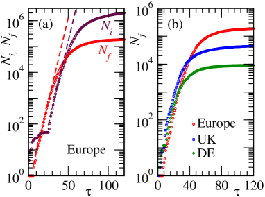
Figure 1: (a) Plots of total number of infections ($N_{i}$) and fatalities ($N_{f}$) in Europe, with the variation of time. A semi-log scale has been chosen. The dashed lines correspond to exponential behavior. (b) Time dependence of fatalities in Europe and two countries within the continent are shown in a semi-log scale.

In Fig. 1 (a) we show, versus time $\tau$, the total numbers of infections and deaths in Europe. This time was counted from the day on which the first cases in respective categories were reported. In both the plots exponential enhancements are visible for significant periods of time, after an onset time $\tau_{0}$. This can be appreciated from the agreements of the data sets with the dashed lines that represent simple exponential growths as in Eq. (1). Fig. 1 (b) shows $N_{f}$, versus $\tau$, from Europe and two countries inside the continent, viz., UK and DE. In the rest of the manuscript all the COVID-19 results will be presented on fatality only.

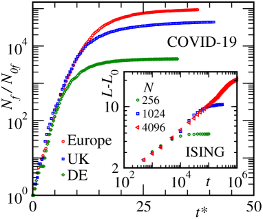
Figure 2: $N_{f}/N_{0f}$, for Europe, DE and UK, are shown with the increase of time, on a semi-log scale. The time here, for each of the regions, has been translated with respect to the value at which a jump, signifying the onset of exponential behavior, was observed. Furthermore, this translated time was scaled via multiplication by appropriately chosen $m_{f}$, value of which is region specific. Inset: Plot of growth data for the Ising model, from different system sizes, on a log-log scale. We have used $L_{0}=1.29$, a value that emerges from the simulations.

In Fig. 2 we show plots of $N_{f}/N_{0f}$, versus translated and scaled time $t^{*}$ [$=m_{f}(\tau-\tau_{0})$], on a semi-log scale. After such transformations early data from different places collapse on top of each other. At late time there is deviation, of course, which is related to the departure from the exponential behavior. The overall picture is analogous to that of kinetics of phase transitions in finite box of different sizes binder2 ; majumder ; majumder2 ; majumder4 . In the latter case data from smaller systems deviate from the thermodynamic limit behavior earlier – see the inset. In the case of disease dynamics the thermodynamic limit (only in the sense of analogy that there is a crossover from this behavior to a saturation at a finite number) behavior mostly comprises of the exponential period.

The main frame of Fig. 3 shows the (finite-size) scaling plot for the disease dynamics. There data from all the above mentioned regions have been included. The collapse appears quite satisfactory, the quality being as good as that for those obtained for phase transitions via computer simulations of simple model systems das0 . This confirms the similarity between the two types of problems. The solid line in this figure represents a power-law with exponent $-1$ that corresponds to $p=1$, i.e., simple exponential behavior at early time. The dashed line there is the analytical function in Eq. (5). The function parameters were obtained by fitting Eq. (5) to the combined data set. For the values see the caption. Near perfect collapse of data from many regions suggest robust universality in the growth dynamics of the disease. Such universality, in spite of the differences in $m_{f}$, that, for the considered places, lies in the range $[0.275,0.35]$ (Europe: $0.32$; DE: $0.275$; NL: $0.33$; IT: $0.325$; ES: $0.315$; UK: $0.35$), suggests that in the post exponential periods the regions are maintaining similar discrepancies with each other as those during the exponential periods. The other best collapse parameters ($N_{0f}$, $N_{df}$) for different regions, in the same sequence as above, are ($2,1500$), ($2,255$), ($1,151$), ($2,545$), ($28,1500$) and ($1,465$).

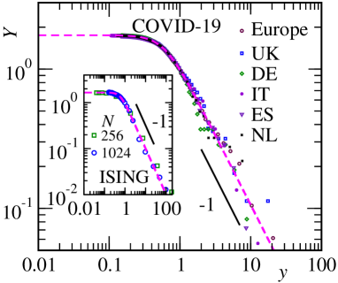
Figure 3: Finite-size scaling exercise for COVID-19 fatalities in a group of regions: $Y$ is plotted versus $y$, on a log-log scale. The solid line is a power-law with exponent $-1$. The dashed line represents the scaling function in Eq. (5) with parameter values $Y_{0}=1.06$, $b=0.23$, $\theta=2.93$, and $p=1.0$. Inset: Here the finite-size scaling function for COVID-19 is compared with the scaled Ising model data for two smallest studied system sizes for which finite-size limits have been reached within the time scales of our simulations. For these systems, i.e., for $N=256$ and $1024$, the obtained values of $L_{\rm max}$, respectively, are $6.2$ and $12$. In this case we have obtained best data collapse for $\alpha=0.3$. Small discrepancy in $\alpha$, from the expected theoretical value of $1/3$, is due to the error in the domain size measurement, owing to thermal noise that has not been eliminated unlike some of our previous studies. Furthermore, for more accurate estimation of $\alpha$ introduction of an instability time $t_{0}$ becomes necessary (see Ref. majumder ).

In the inset of Fig. 3 we have shown the analogous scaling plot by using data from the simulations of the Ising model. There it is clearly seen that the phase transition data are very nicely described by the analytical function for the disease. This observation combines the uniqueness in the disease spread with phase transition, except for the fact that in one case to get the actual number one needs to go through an exponential transformation and in the other case an algebraic transformation is necessary. It is worth mentioning here, even though we have shown results for six regions, we believe that data from more countries will be described by the same analytical function. In the phase transition scenario also, universality in finite-size scaling behavior is broad – this combines the considered Ising model with coarsening scenario in multi-component mixtures and fluid systems das0 ; majumder2 ; majumder4 . For the latter, neither the scaling function was previously derived nor such an agreement was obtained with a construction of any type.

The parameters that decide the universality in disease dynamics are $p$ and $\theta$. The others are simple multiplicative factors. Between $p$ and $\theta$, it has already been observed that $p=1$, i.e., early behavior is practically simple exponential. Thus, $\theta$ is the quantity to look for. Note that for the Ising case, independent fitting to the combined scaling plot provides $\theta=2.29$, for $p=1$. While this is only about $20$% less than the COVID-19 value, in a less restricted sense the universality can be classified in accordance with power-law or exponential behavior of $f(y)$.

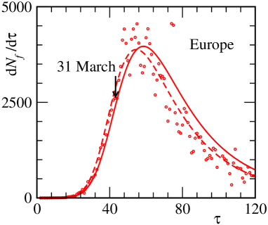
Figure 4: Symbols represent the daily deaths, due to COVID-19, in Europe for a period of 120 days, starting from $27$ January. The dashed line is obtained from the scaling function in Fig. 3. The continuous line is obtained by fitting only the data of Europe till $31$ March, by fixing $\theta$ at $3$, approximately the number for the scaling function in Fig. 3.

In Fig. 4 we have demonstrated the predictive capability of the scaling model. There we have compared the real data for daily new deaths in Europe with the analytical description. The connection between $Y$ and $N_{f}$ has already been mentioned above. The dashed line in this figure represents analytical function obtained by fitting to the full combined data set in Fig. 3. Obviously, the agreement is very good. For the prediction purpose, however, we have fitted the data for Europe only till March 31, a date that is significantly earlier than the appearance of the peak in this continent. Again the agreement is good. Certainly, then, the model has strong predictive character.

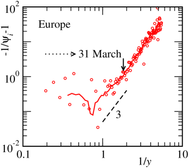
Figure 5: Dependence of $\psi_{i}$, the instantaneous exponent, on $y$ is demonstrated, on a double-log scale, for Europe. The dashed line represents $\theta=3.0$. The arrow-headed solid line points to the date $31$ March. The arrow-headed dotted line shows the direction of increasing time. The continuous line represents running averaged plot of the original data that are shown using symbols.

In the fitting of the data for Europe till 31 March, we had fixed the value of $\theta$ at $3$, approximately the number that is obtained for $\theta$ by fitting the combined full data set in Fig. 3. The justification is provided below. Dependence of $\psi_{i}$ on $y$ is shown in Fig. 5. The number obtained by fitting the combined data is consistent with the actual scenario. Furthermore, by $31$ March, a steady picture, consistent with the above mentioned exponent, has already emerged. This tells about the reason behind such a good prediction. The overall story essentially conveys that a unique pattern for the disease dynamics for many places emerges rather early. Once this is captured, action on SR and various facilities becomes easier.

IV Conclusion

We have studied real data wiki concerning fatality due to COVID-19 in a group of regions. A finite-size-like scaling model fisher3 ; book1 ; binder2 ; majumder ; majumder2 ; majumder4 ; das0 , analogous to the one used for studies of phase transitions in small boxes, has been applied. Analysis via this model suggests that the growth in fatality occurs exponentially fast at early time. The model nicely combines this with the behavior at late time and suggests that there exists strong universality skd_spread ; jkb . It has been shown that the coarsening behavior during phase transitions book1 follow the analogous scaling pattern when studied in finite boxes binder2 ; majumder ; majumder2 ; das0 .

An empirically derived finite-size scaling function skd_spread describes the disease growth as well as domain growth during phase transitions quite accurately. The scaling function, and, thus, the model, has predictive power. This has been demonstrated by analyzing data over a small early time window and comparing the analytical function for the time dependence of $N_{f}$, thus obtained, with the future of the disease dynamics. The construction of the function does not put restriction on the very early-time monotonicity. However, for a pure exponential behavior it is necessary. This feature of the function may lead to errors if the data are very noisy. However, conditions can be imposed to get rid of such errors.

Error free predictions indeed require high quality early time data. An improvement by statistical averaging is not possible with real data, as far as the spread of a disease is concerned. Nevertheless, models can be constructed sourav0 to replicate, in a statistical sense, the ground data, providing scope for improvement by averaging over many such trials. We are interested in devising such combined methods sourav1

Acknowledgment: The author acknowledges financial supports from the Department of Biotechnology, India (grant No. LSRET-JNC/SKD/4539); and Science and Engineering Research Board of Department of Science and Technology, India (grant No. MTR/2019/001585). He is thankful to F. Müller-Plathe for important queries and to K. Dey for a help with the bibliography.

Data accessibility: This article has no additional data.

Authors’ Contributions: S.K.D. designed the problem, carried out the work and wrote the manuscript.

The authors declares that there is no competing interest.

^∗ das@jncasr.ac.in

References

- (1) https://en.wikipedia.org/wiki/COVID-19-pandemic. The disease data were collected in 2020.
- (2) M.U.G. Kraemer et al., The effect of human mobility and control measures on the COVID-19 epidemic in China, Science 368, 493 (2020).
- (3) H. Tian et al., An investigation of transmission control measures during the first 50 days of the COVID-19 epidemic in China, Science 368, 638 (2020).
- (4) C. Manchein et al., Strong correlations between power-law growth of COVID-19 in four continents and the inefficiency of soft quarantine strategies, Chaos 30, 041102 (2020).
- (5) J. Lammers, J. Crusius, and A. Gast, Correcting misperceptions of exponential coronavirus growth increases support for social distancing, Proc. Natl. Acad. Sci. USA 117, 16264 (2020).
- (6) D. Adam, The simulations driving the world’s response to COVID-19, Nature 580, 316 (2020).
- (7) C. Fraser, S. Riley, A. Meeyai, S. Iamsirithaworn, and D.S. Burke, Strategies for containing an emerging influenza pandemic in Southeast Asia, Nature 437, 209 (2020).
- (8) Y. Ma et al., Effects of temperature and humidity on the daily new cases and new deaths of COVID-19 in 166 countries, Sci. Tot. Environ. 724, 138226 (2020).
- (9) S.K. Das, A scaling investigation of pattern in the spread of COVID-19: universality in real data and a predictive analytical description, Proc. R. Soc. A 477, 20200689 (2021).
- (10) W.O. Kermack and A.G. McKendrick, A contribution to the mathematical theory of epidemics, Proc. R. Soc. A 115, 700 (1927).
- (11) R.M. Anderson, In population dynamics of infectious diseases: theory and applications, in Population Dynamics of Infectious Diseases: Theory and Applications, edited by R.M. Anderson (Chapman and Hall, NewYork, 1982), pp. 1- 37.
- (12) C.M. Schneider, T. Mihaljev, S. Havlin, and H.J. Herrman, Suppressing epidemics with a limited amount of immunization units, Phys. Rev. E 84, 061911 (2011).
- (13) M.E. Fisher, The theory of equilibrium critical phenomenon, Rep. Prog. Phys. 30, 615 (1967).
- (14) A. Onuki, Phase Transition Dynamics (Cambridge University Press, Cambridge, England, 2002).
- (15) A.J. Bray, Theory of phase-ordering kinetics, Adv. Phys. 51, 481 (2002).
- (16) M.E. Fisher and M.N. Barber, Scaling theory for finite-size effects in the critical region, Phys. Rev. Lett. 28, 1516 (1972).
- (17) K. Binder and D.P. Landau, A guide to Monte Carlo simulations in statistical physics (Cambridge University Press, Cambridge, 2009).
- (18) S.K. Das, M.E. Fisher, J.V. Sengers, J. Horbach, and K. Binder, Critical Dynamics in a Binary Fluid: simulations and Finite-Size Scaling, Phys. Rev. Lett. 97, 025702 (2006).
- (19) D.W. Heermann, L. Yixue, and K. Binder, Scaling solutions and finite-size effects in the Lifshitz-Slyozov theory, Physica A 230, 132 (1996).
- (20) S. Majumder and S.K. Das, Diffusive domain coarsening: early time dynamics and finite-size effects, Phys. Rev. E 84, 021110 (2011).
- (21) S. Majumder and S.K. Das, Temperature and composition dependence of kinetics of phase separation in solid binary mixtures, Phys. Chem. Chem. Phys. 15, 13209 (2013).
- (22) S.K. Das, S. Roy, S. Majumder and S. Ahmad, Finite-size effects in dynamics: critical vs. coarsening phenomena, Europhys. Lett. 97, 66006 (2012).
- (23) S. Majumder, J. Zierenberg, and W. Janke, Kinetics of polymer collapse: effect of temperature on cluster growth and aging, Soft Matter 13, 1276 (2017).
- (24) S. Majumder, S.K. Das, and W. Janke, Universal finite-size scaling function for kinetics of phase separation in mixtures with varying number of components, Phys. Rev. E 98, 042142 (2018).
- (25) H. W. Hethcote, The Mathematics of Infectious Diseases, SIAM Rev. 42, 599 (2000).
- (26) G. M. Viswanathan, M. G. E. da Luz, E. P. Raposo, and H. E. Stanley, The physics of foraging: an introduction to random searches and biological encounters (Cambridge University Press, 2011).
- (27) N. Harding, R. Nigmatullin, and M. Prokopenko, Thermodynamic efficiency of contagions: a statistical mechanical analysis of the SIS epidemic model, Interface Focus 8, 0036 (2018).
- (28) I.M. Lifshitz and V.V. Slyozov, The kinetics of precipitation from supersaturated solid solutions, J. Phys. Chem. Solids 19, 35 (1961).
- (29) D.A. Huse, Corrections to late-stage behavior in spinodal decomposition: Lifshitz-Slyozov scaling and Monte Carlo simulations, Phys. Rev. B 34, 7845 (1986).
- (30) J.G. Amar, F.E. Sullivan, and R.D. Mountain, Monte Carlo study of growth in the two-dimensional spin-exchange kinetic Ising model, Phys. Rev. B 37, 196 (1988).
- (31) A. Paul, J.K. Bhattacharjee, A. Pal, and S. Chakraborty, Emergence of universality in the transmission dynamics of COVID-19, Sci. Rep. 11, 18891 (2021).
- (32) S. Chowdhury, S. Roychowdhury and I. Choudhuri, Cellular automata in the light of COVID-19, Eur. Phys. J. Spl. Topics 231, 3619 (2023).
- (33) S. Chowdhury, S. Roychowdhury, I. Choudhuri and S.K. Das, work in progress.