Quantum phase transitions and cat states in cavity-coupled quantum dots

Abstract

We study double quantum dots coupled to a quasistatic cavity mode with high mode-volume compression allowing for strong light-matter coupling. Besides the cavity-mediated interaction, electrons in different double quantum dots interact with each other via dipole-dipole (Coulomb) interaction. For attractive dipolar interaction, a cavity-induced ferroelectric quantum phase transition emerges leading to ordered dipole moments. Surprisingly, we find that the phase transition can be either continuous or discontinuous, depending on the ratio between the strengths of cavity-mediated and Coulomb interactions. We show that, in the strong coupling regime, both the ground and the first excited states of an array of double quantum dots are squeezed Schrödinger cat states. Such states are actively discussed as high-fidelity qubits for quantum computing, and thus our proposal provides a platform for semiconductor implementation of such qubits. We also calculate gauge-invariant observables such as the net dipole moment, the optical conductivity, and the absorption spectrum beyond the semiclassical approximation.

Introduction. Placing condensed matter systems in an optical cavity is a promising way of engineering new correlated states of matter via the interaction with quantum fluctuations of the cavity field [1]. The main experimental challenge is to achieve the ultrastrong light-matter coupling regime [2, 3] that can be reached by external driving [4, 5, 6, 7, 8, 9, 10], by tuning the cavity in a plasmon or an exciton-polariton resonance [11], or by compressing down the effective mode volume in specially designed resonators [12, 13] that can be thought of as an $LC$-circuit [14, 15] with a single discrete quasistatic mode, whose frequency $\omega_{0}=1/\sqrt{LC}$ is not constrained by the resonator dimensions. When the light-matter coupling is strong enough, then even in the ground state the vacuum fluctuations can radically modify electron systems [16, 17]. This phenomenon fosters a qualitatively new class of condensed-matter platforms with strongly correlated light-matter excitations.

Superradiance, initially described by R. H. Dicke [18, 19], has garnered significant attention to coupled light-matter systems ever since. There exist various effective models describing electron systems coupled to a cavity, known as extended and generalized Dicke models, see, e.g., Refs. [20, 21, 22, 23]. An important restriction to such effective models is the gauge invariance that must be preserved [24] when perturbation theory or Hilbert space truncation is employed. Originally, the main signature of the superradiant Dicke phase transition was a photon condensate, the macroscopic occupation of the cavity mode that is not gauge-invariant [25]. Nevertheless, the quantum phase transition is present and equivalent to the ferroelectric phase transition (FPT), resulting in ordered electric dipole moments, see Refs. [26, 27]. Important, the FPT is only possible if the Coulomb interaction between the dipoles is included [28, 29, 21, 26, 30].

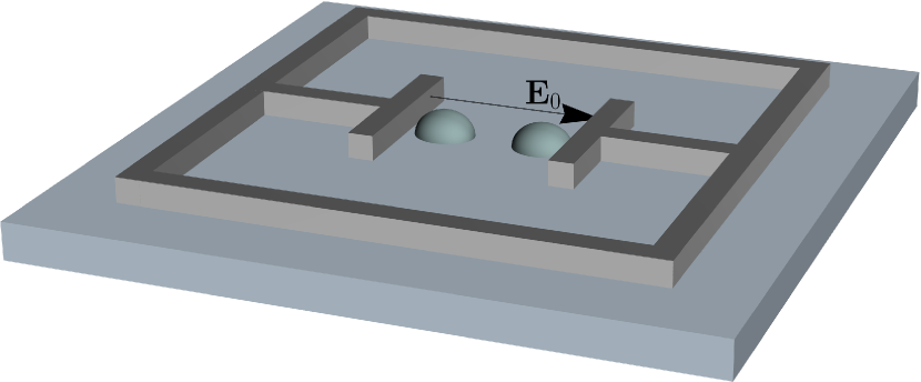
Figure 1: (a) Sketch of the system: Two DQDs embedded in a split-ring resonator. The cavity mode is polarized along the arrow, $\mathbf{E}_{0}=(0,0,E_{0})$. (b) Two double-well potentials for each DQD. The two lowest energy levels are shown. The two minima of each DQD are marked with L (Left) and R (Right), respectively. The DQD axes are aligned along the $z$ axis.

In this work, we consider a few cavity-coupled double quantum dots (DQDs) with a Coulomb interaction between them, the only non-trivial part of which is the electric dipole-dipole interaction. Choosing a geometry where the dipolar interaction between DQDs is attractive, we find a FPT of the first or second order depending on the relative strength of the Coulomb and light-matter interactions, leading to ordered phases of the electric dipole moments. Most importantly, the ground state and the first excited state in the ferroelectric phase in the strong coupling regime are squeezed Schrödinger cat states. In particular, this is true already for two cavity-coupled DQDs with attractive dipole-dipole (Coulomb) interaction. We suggest such systems as possible semiconductor candidates for a self-correcting cat qubit [31, 32] and a realistic platform to study cavity-induced quantum phase transitions. Here we calculate the net dipole moment, the optical conductivity, and the absorption spectrum all of which are gauge-invariant.

Model. A few identical singly-occupied DQDs are oriented along the line connecting the capacitor plates as shown in Fig. 1. Due to the Coulomb repulsion, DQDs interact with each other directly via the electric dipole-dipole interaction. The double-well shape of the confining potential of each DQD allows us to truncate electron energy levels by the lowest two as long as the higher states are far detuned [33, 34]. Such an electronic system is described by the following Hamiltonian, ${H}_{\text{el}}=-(\Delta/2)\sum_{i=1}^{N}\left({c}_{i,L}^{\dagger}{c}_{i,R}+\text{h.c.}\right)+\sum_{i>j}^{N}(U_{ij}/2){d}_{i,z}{d}_{j,z}-(V_{b}/2)\sum_{i=1}^{N}{d}_{i,z}$, where ${c}^{\dagger}_{i,L/R}$ (${c}_{i,L/R}$) are the electron creation (annihilation) operators for the two sites ($L/R$) of the i^th DQD, $N$ is number of DQDs, $V_{b}$ the bias along the DQD axis, $\Delta/2$ the DQD level hybridization, and ${d}_{i,z}={c}^{\dagger}_{i,R}{c}_{i,R}-{c}^{\dagger}_{i,L}{c}_{i,L}$ the electric dipole operator. Spin indices are suppressed. The Coulomb interaction is reduced to the dipole-dipole interaction here due to the two-level truncation of each singly-occupied DQD. The dipolar interaction strength between two DQDs is given by $U_{ij}/2\approx(eb/2)^{2}(|\mathbf{r}_{ij}|^{2}-3(\mathbf{r}_{ij}\cdot\mathbf{e}_{z})^{2})/(\varepsilon|\mathbf{r}_{ij}|^{5})$, where $\mathbf{r}_{ij}$ is the distance vector between two DQD centers, $\varepsilon$ the dielectric constant, $e<0$ the elementary charge, $b$ the DQD length, and $eb/2$ the dipole matrix element between the lowest two levels of a DQD. If DQDs are assembled along the capacitor axis $z$, the dipole-dipole interaction is attractive, $U_{ij}=-(eb)^{2}/(\varepsilon r_{ij}^{3})<0$ with $\bm{r}_{ij}=r_{ij}\mathbf{e}_{z}$ being the distance vector between two DQD centers. Screening of $U_{ij}$ due to proximity to the capacitor plates does not affect the sign of $U_{ij}$ but only slightly modifies its absolute value. In what follows, we mostly focus on two ($N=2$) DQDs. In this case, only the $U_{12}\equiv U$ matrix element of the dipole-dipole interaction is important. Throughout the paper, we use cgs-units and also set the Planck and Boltzmann constants to unity, $\hbar=k_{B}=1$.

All DQDs are coupled to a single quantized quasistatic $LC$-cavity mode [35, 36, 37]. The quantized electric field of the cavity mode is almost completely localized in the capacitor and polarized along the line connecting the DQDs, see Fig. 1. The corresponding vector-potential operator ${A}_{z}$ is given by ${A}_{z}=iE_{0}/\omega_{0}({a}^{\dagger}-{a})\equiv i\sqrt{2\pi/(\varepsilon V_{\text{eff}}\,\omega_{0})}({a}^{\dagger}-{a})$, where $a$ ($a^{\dagger}$) is the annihilation (creation) operator of the cavity mode with frequency $\omega_{0}$, $E_{0}$ the amplitude of the electric field fluctuations, and $V_{\text{eff}}$ the effective mode volume.

\begin{overpic}[scale={0.4}]{fig_energy_spectum_2nd_order_qpt.pdf} \put(57.0,12.0){\includegraphics[scale={0.133}]{fig_d2Eoverdg2_inset.pdf}} \end{overpic}

Figure 2: Exact energy spectrum of $H$ given in Eq. (2) for $\omega_{0}/\Delta=0.1$, and attractive dipolar interaction (a) $U/\omega_{0}=-5$, (b) $U/\omega_{0}=-1.5$ as function of light-matter coupling constant $g$. The six lowest energy levels are shown. The FPT is second-order in panel (a) and first-order in panel (b). In (b), the ferroelectric (trivial) phase is on the right (left) side of the vertical dashed red line indicating the FPT. The insets show the (a) second and (b) first derivatives of the ground state energy $E_{\text{GS}}(g)$ obtained by the exact diagonalization (ED). In the inset in (a) the bump converges in the quasi-thermodynamic limit $\omega_{0}/\Delta\to 0$ to the jump predicted by the semi-classical result (SM, solid curve), whereas in (b) the jump occurs without the need to take the limit. Both jumps are followed by a ferroelectric phase.

We couple the DQDs to the cavity via the Peierls substitution,

$${H}_{0}=\omega_{0}{a}^{\dagger}{a}-V_{b}{S}_{z}+U{S}_{z}^{2},$$ (1)

$${H}={H}_{0}-\frac{\Delta}{2}\left(e^{g(a-a^{\dagger})}{S}_{+}+e^{-g(a-a^{\dagger})}{S}_{-}\right),$$ (2)

$$g=\sqrt{\frac{W}{\omega_{0}}}\,,\hskip 5.0ptW=\frac{2\pi e^{2}b^{2}}{\varepsilon V_{\text{eff}}},$$ (3)

where ${S}_{\beta}=1/2\sum_{i=1}^{N}\sigma_{i,\beta}$ is the orbital pseudospin of the system, $\sigma_{i,\beta}$ is the Pauli matrix corresponding to the $i^{\rm th}$ DQD, $\beta\in\{x,y,z\}$, $g$ is the dimensionless light-matter coupling constant, $U_{ij}=U$. The operators ${S}_{z}$ and ${S}_{\pm}={S}_{x}\pm i{S}_{y}$ satisfy the standard spin algebra: $[{S}_{\pm},{S}_{z}]=\mp{S}_{\pm}$, $[{S}_{+},{S}_{-}]=2{S}_{z}$. The pseudospin ${\bm{S}}$ describes the collective orbital degree of freedom in the DQD array. For example, the total dipole moment operator maps onto ${S}_{z}$: $\sum_{i=1}^{N}{d}_{i,z}\to 2{S}_{z}$.

Figure 3: (a) Phase diagram of the numerically exact net dipole moment $\langle{S}_{z}\rangle$ for $N=2$ DQDs at $\omega_{0}/\Delta=0.1$ and zero temperature as function of the dipole interaction strength $U$ and light-matter coupling constant $g$. An infinitesimal symmetry-breaking field $-V_{b}{S}_{z}$ with $V_{b}/\omega_{0}=10^{-4}$ is introduced. The FPT is first (second) order at $|U|/\omega_{0}\lesssim 2$ ($|U|/\omega_{0}\gtrsim 2$), and the star marks the critical point, $|U|/\omega_{0}\approx 2$, separating two different types of phase transitions. (b) Phase diagram of $\langle{S}_{z}^{2}\rangle$ at finite temperature $T/\omega_{0}=0.1$.

First, we diagonalize the Hamiltonian $H$, see Eq. (2), numerically for $N=2$ cavity-coupled DQDs at zero bias $V_{b}=0$. The first six energy levels are shown in Fig. 2. We analyze the system in the quasi-thermodynamic limit $\omega_{0}\ll\Delta$ (the limit of the classical oscillator), see Refs. [38, 39, 40, 41] for details. We find the FPT for any attractive dipole-dipole interaction $U<0$ and large enough light-matter coupling $g$. A 2D plot of the net dipole moment $\langle{S}_{z}\rangle$ as a function of ($g$,$U/\omega_{0}$) at $\omega_{0}/\Delta=0.1$ and zero temperature [see Fig. 3(a)] shows the FPT of second (first) order at $|U|/\omega_{0}\gtrsim 2$ ($|U|/\omega_{0}\lesssim 2$). These two regimes are separated by the critical point located at $|U|/\omega_{0}\approx 2$, the green star in Fig. 3(a). At finite temperature, the FPT turns into a cross-over, see the density plot of $\langle{S}_{z}^{2}\rangle$ in Fig. 3(b). We note that $\langle S_{z}^{2}\rangle$ is meaningful for $N\geq 2$ DQDs. In contrast to $\langle S_{z}\rangle$, $\langle S_{z}^{2}\rangle$ is not sensitive to small symmetry breaking field $V_{b}$ which is useful at finite temperatures $T\gg|V_{b}|$. Interestingly, a single cavity-coupled DQD shows the cavity-induced FPT at strong coupling [40], whereas two DQDs do not unless there is an attractive dipolar interaction between them. In contrast to the Dicke- and Rabi- models predicting the second-order FPT, here we observe the first-order FPT that is not sensitive to the quasi-thermodynamic limit.

Photonic semi-classical decoupling. In order to gain physical insight into our numerical results, we apply the semi-classical approximation to photons while keeping the orbital pseudospin ${\bm{S}}$ quantum. The photonic semi-classical decoupling is reminiscent of the length gauge formulation of the problem [42, 43, 44, 45],

$${H}_{\text{D}}={U}{H}{U}^{\dagger}={H}_{\text{sm}}+\delta{V},$$ (4)

$${H}_{\text{sm}}=\omega_{0}{a}^{\dagger}{a}-V_{b}{S}_{z}-\Delta{S}_{x}+U{S}_{z}^{2}+g^{2}\omega_{0}\left(\delta{S}_{z}\right)^{2},$$ (5)

$$\delta{V}=-g\omega_{0}\,\delta{S}_{z}\left({a}+{a}^{\dagger}\right),$$ (6)

where ${H}$ is given by Eq. (2), ${U}=\exp{\left[g\,\delta{S}_{z}({a}^{\dagger}-{a})\right]}$, $\delta{S}_{z}={S}_{z}-\langle{S}_{z}\rangle$, $\langle{S}_{z}\rangle$ is the average of orbital pseudospin ${S}_{z}$ over the ground state of the semi-classical Hamiltonian ${H}_{\text{sm}}$. The perturbation $\delta{V}$ accounts for quantum corrections beyond the semi-classical approximation. In contrast to conventional mean-field treatment where both, the photons and the pseudospin, are treated as classical objects, see e.g. Ref. [38], the orbital pseudospin ${\bm{S}}$ in our work remains quantum because we apply our results to a small number of DQDs.

The Hamiltonian ${H}_{D}$ commutes with ${\bm{S}}^{2}$, so we consider states with definite orbital pseudospin $S$. Single DQD corresponds to $N=1$ and $S=1/2$, this case is known as the Rabi model [40]. In case of $N=2$ DQDs, see Fig. 1, $S$ can be either $0$ or $1$. The $S=0$ state does not couple to the antenna. If $S=1$, the semi-classical Hamiltonian [Eq. (5)] can be diagonalized analytically, see the SM [46]. Here, we show the semi-classical ground-state energy, $E_{\text{sm}}$, of two cavity-coupled DQDs at $V_{b}=0$ (symmetric DQDs):

$$E_{\text{sm}}=-\frac{2}{3}\sqrt{P}\cos\left[\arccos\left(Q/P^{3/2}\right)/3\right]$$

$$+\frac{2}{3}\left(U+g^{2}\omega_{0}\right)+\omega_{0}\alpha^{2},$$ (7)

where $P$ and $Q$ are defined as follows,

$$P=\left(U+g^{2}\omega_{0}\right)^{2}+3\left(\Delta^{2}+4g^{2}\alpha^{2}\omega_{0}^{2}\right),$$ (8)

$$Q=\left(U+g^{2}\omega_{0}\right)\left[\left(U+g^{2}\omega_{0}\right)^{2}-36\alpha^{2}g^{2}\omega_{0}^{2}+9\Delta^{2}/2\right].$$

Here, we introduced the parameter $\alpha=g\langle{S}_{z}\rangle$. If $\alpha=0$, the phase is trivial. If $\alpha\neq 0$, the ground state is ferroelectric, i.e., it has a net dipole moment $\langle{S}_{z}\rangle\neq 0$. The FPT between the trivial and the ferroelectric phases is first (second) order if $\langle{S}_{z}\rangle$ has a finite jump (continuous) at the transition, see Fig. 3(a).

As $E_{\text{sm}}$ is an even function of $\alpha$ at $V_{b}=0$ [Eq. (7)], the ground state of ${H}_{\text{sm}}$ is two-fold degenerate at $\alpha\neq 0$. This degeneracy is best seen from the symmetry $\mathcal{P}=\exp(i\pi{a}^{\dagger}{a}+i\pi{S}_{x})$ of the transformed Hamiltonian ${H}_{T}={T}(\alpha){H}_{D}{T^{\dagger}}(\alpha)$ at $V_{b}=0$, where ${T}(\alpha)=e^{\alpha({a}^{\dagger}-{a})}$. Note that ${T}(\alpha)$ is the optical displacement operator that creates the coherent state $|\alpha\rangle={T}(\alpha)|0\rangle$, where $|0\rangle$ is the photonic vacuum of ${H}_{\text{sm}}$, see Eq. (5). While the symmetry breaking in this problem occurs only in the limit $\omega_{0}/\Delta\to 0$, we expect very small lifting of the degeneracy at any finite $\omega_{0}/\Delta\ll 1$ such that the parity symmetry $\mathcal{P}$ of the Hamiltonian ${H}_{T}$ is restored. In particular, the ground state, $|\Psi_{\text{G}}\rangle$, and the first excited state, $|\Psi_{\text{E1}}\rangle$, of the Hamiltonian ${H}_{T}$ in the semi-classical approximation correspond to $\mathcal{P}=+1$ and $\mathcal{P}=-1$, respectively

$$|\Psi_{\text{G}}\rangle=\mathcal{N}\left[\chi(\alpha)|\alpha\rangle+\chi(-\alpha)|-\alpha\rangle\right],$$ (9)

$$|\Psi_{\text{E1}}\rangle=\mathcal{N}\left[\chi(\alpha)|\alpha\rangle-\chi(-\alpha)|-\alpha\rangle\right],$$ (10)

where $\alpha>0$ corresponds to positive dipole moment $\langle{S}_{z}\rangle>0$, $|\alpha\rangle={T}(\alpha)|0\rangle$ is the photonic coherent state, $\chi(\pm\alpha)$ are the two lowest-energy eigenstates of ${H}_{\text{sm}}$, and $\mathcal{N}$ is the normalization factor. Indeed, we observe a finite splitting in the ferroelectric phase, see Fig. 2(a). Restoration of the parity symmetry $\mathcal{P}$ is due to the tunneling (instantons) between two semi-classical ground states [47].

\begin{overpic}[scale={0.4}]{fig_fidelity.pdf} \put(51.0,13.0){\includegraphics[scale={0.19}]{fig_cat_size.pdf}} \end{overpic}

Figure 4: Fidelities $|\langle\text{GS}\lvert\Psi_{\text{G}}\rangle|$ and $|\langle\text{E1}\lvert\Psi_{\text{E1}}\rangle|$ in the ferroelectric phase as function of light-matter coupling $g$, where $|\text{GS}\rangle$ and $|\text{E1}\rangle$ are the exact ground state and the first excited state, $\lvert\Psi_{\text{G}}\rangle$ and $\lvert\Psi_{\text{E1}}\rangle$ are the semi-classical cat states, see Eqs. (9), (10). The semi-classical approximation is valid if the fidelities are close to one. The following parameters are used: the dipole-dipole interaction strength is $U/\omega_{0}=-5$ and $\omega_{0}/\Delta=0.1$. The inset shows the “cat size” $\alpha^{2}$.

The fidelities $|\langle\text{GS}\lvert\Psi_{\text{G}}\rangle|$ and $|\langle\text{E1}\lvert\Psi_{\text{E1}}\rangle|$ plotted in Fig. 4 as function of $g$ justify the semi-classical treatment in the ferroelectric phase, where $|\text{GS}\rangle$ and $|\text{E1}\rangle$ are exact (numerical) ground and first excited states, $\lvert\Psi_{\text{G}}\rangle$ and $\lvert\Psi_{\text{E1}}\rangle$ are corresponding semi-classical cat states, see Eqs. (9) and (10). This confirms the semiclassical result that the ground and the first excited states are two-component squeezed (due to effective photon nonlinearity [48]) Schrödinger cat states. The parameter $\alpha^{2}$, being an increasing function of $g$ (see the inset in Fig. 4), plays the role of the “cat size”. The comparison between the semi-classically calculated phase diagram for the order parameter $\langle\hat{S}_{z}^{2}\rangle$ and the exact diagonalization is shown in SM [46]. Two lowest energy levels become degenerate in the strong coupling limit $g\to+\infty$, see Fig. 2, when the Schrödinger cats become truly classical. In order to use such a system as a cat qubit, a finite energy splitting is required, which restricts the cat size $\alpha^{2}$. On the bright side, the cat states appearing in the ultrastrong coupling regime of a somewhat similar quantum Rabi model are robust to decoherence and can be harnessed to implement quantum gates with high fidelity [49, 50]. We propose the cavity-coupled DQDs as a new solid-state platform for cat qubits, as promising candidates for quantum computing [51, 51]. In contrast to atomic systems (e.g., see [52, 53, 54]), solid-state platforms are scalable and require much less stringent experimental conditions. In contrast to previous proposals based on quantum dots [55], our model does not require external driving. Also the fact that we have several DQDs results in greater resilience to noise.

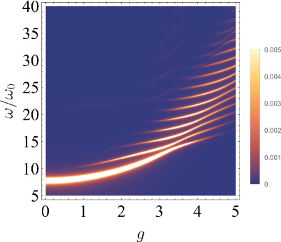
Figure 5: Density plot of (a) the optical conductivity $\operatorname{Re}\left[\sigma(\omega)\right]/\sigma_{0}$ and (b) the absorption spectrum (photon spectral function) for $N=2$ DQDs at $U/\omega_{0}=-5$ and $\omega_{0}/\Delta=0.1$. The optical conductivity shows a frequency comb (light stripes) at strong coupling. The normalization parameter $\sigma_{0}=(eb)^{2}$ and each delta peak is replaced by a Lorentzian with the broadening $\Gamma/\omega_{0}=0.1$. The absorption spectrum shows the lower polariton softening alongside a reduction in its spectral weight.

Optical conductivity and absorption spectrum. Two gauge invariant response functions that can be routinely measured are the optical conductivity and the absorption spectrum. The latter is defined [56] as the cavity response to an AC voltage applied to the cavity and is proportional to the Fourier transform of $C(t)=\langle{A}_{z}(t){A}_{z}(0)\rangle$. The absorption spectrum was thoroughly studied before [57, 14, 58] as a function of the driving frequency, showing two standard polariton branches. We plot the absorption spectrum in Fig. 5(b), revealing the softening of the lower polariton mode to zero during the second-order FPT. Importantly, the previous studies of cavity-embedded semiconductor systems [14] did not reveal quantum phase transitions due to the lack of engineering of the Coulomb interaction between individual dipoles, which is problematic to achieve with quantum wells.

The optical conductivity is calculated by standard means [59]

$$\operatorname{Re}\left[\sigma(\omega)\right]=\frac{1}{2\omega}\int_{-\infty}^{+\infty}dte^{i\omega t}\langle{J}(t){J}\rangle,$$ (11)

where the current operator ${J}$ along the DQD axis is defined as ${J}=e\,d{z}/dt=i\left[{H}_{D},(eb/2)\sum_{i}{d}_{i,z}\right]$ because the ${z}$ coordinate operator is replaced by the dipole moment, and in the length gauge [Eq.(4)] is given by $J=i\left[H_{D},ebS_{z}\right]=-eb\Delta S_{y}$.

Contrary to absorption, the optical conductivity retains a strong frequency comb deep in the ferroelectric phase, see Fig. 5(a). We stress that such a frequency comb is not present in the semi-classical approximation, see Eq. (5). Here, we present analytic result for $\operatorname{Re}\left[\sigma(\omega)\right]$,

$$\operatorname{Re}\left[\sigma(\omega)\right]\approx\frac{\pi S}{2\omega}\left(eb\Delta\right)^{2}\sum\limits_{n=0}^{\infty}p_{n}(g^{2})\delta\left(\omega-E_{n}\right),$$ (12)

where $S$ is the pseudospin, $p_{n}(z)=e^{-z}z^{n}/n!$ is the Poisson distribution, and $E_{n}=n\omega_{0}-U(2S-1)$. Equation (12) is valid in the ferroelectric phase at arbitrary $g$ and near-full semi-classical polarization $|\langle S_{z}\rangle|\approx S$, see the SM [46] for details. Interestingly, the Poissonian structure of the frequency comb in $\operatorname{Re}\left[\sigma(\omega)\right]$ is similar to replica bands recently discussed in the context of light-matter interaction [60].

To demonstrate that our findings are of relevance for state-of-the-art experiments, we provide typical parameters: $\omega_{0}$ ranges from tens of GHz to tens THz (i.e. $\omega_{0}\sim 0.01-10$ meV). The splitting between the quantum dots can vary between $\Delta\sim 0.1-10$ meV. The magnitude of electrostatic dipole-dipole interaction strength $|U|$ depends on the quantum dot configuration (sizes, distance, and mutual orientation), and can be tuned in the range from $0-10$ meV. The light-matter interaction strength $g$ can be tuned in a vast range and greatly exceed unity for typical semiconductor double quantum dots if the mode volume is made small enough. Thus, the parameters presented on the plots are well within the experimentally accessible range.

Conclusion. We analyzed a small array of DQDs coupled to a single $LC$-cavity. We find a FPT at strong light-matter coupling and attractive dipole-dipole interaction between DQDs due to the Coulomb force. The FPT is either first or second order depending on the dipole-dipole interaction strength. The first-order FPT is due to the interplay between the cavity-mediated interactions and the dipole-dipole interaction of the Coulomb nature. We show that the ground state and the first excited state of two cavity-coupled DQDs in the ferroelectric phase are Schrödinger-cat states. We argue that such cavity-coupled DQD systems can be used as cat qubits that are actively discussed as an alternative to spin qubits. Higher energy excited states can be studied via the optical conductivity spectra that demonstrate dense frequency comb in the strong coupling limit.

Supplemental material: “Quantum phase transitions and cat states in cavity-coupled quantum dots”

I Semiclassical analysis

The semiclassical Hamiltonian $H_{\text{sm}}$ takes the following form

$$H_{\text{sm}}=\omega_{0}a^{\dagger}a-V_{b}S_{z}-\Delta S_{x}+US_{z}^{2}+g^{2}\omega_{0}\left(\delta S_{z}\right)^{2},$$ (13)

where $\delta S_{z}=S_{z}-\langle S_{z}\rangle$, $\langle S_{z}\rangle$ is the average of $S_{z}$ over the ground state of $H_{\text{sm}}$. Within this approximation, photons are decoupled from the orbital pseudospin, so the semiclassical ground state wave function $\Psi_{\text{sm}}=|0\rangle\chi_{\text{sm}}$, where $|0\rangle$ is the photon vacuum, $\chi_{\text{sm}}$ is the lowest-energy spinor of $\langle 0|H_{\text{sm}}|0\rangle$. The semiclassical ground-state energy $E_{\text{sm}}$ follows from the characteristic equation $\det(\langle 0|H_{\text{sm}}|0\rangle-E_{\text{sm}})=0$.

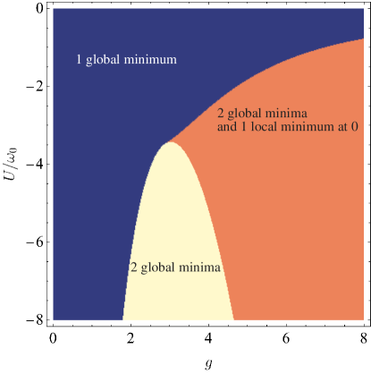
Figure 6: Energy landscape of the semiclassical ground state at $\omega_{0}/\Delta=0.1$. Blue region : the semiclassical lowest energy $E_{\text{sm}}(\alpha)$ has its minimum at $\alpha=0$. Yellow region: the semiclassical energy $E_{\text{sm}}(\alpha)$ has the two minima $\pm\alpha\neq 0$, and $E^{\prime\prime}_{\text{sm}}(\alpha=0)<0$. Orange region: the semiclassical energy has the two minima at $\pm\alpha\neq 0$, and $E^{\prime\prime}_{\text{sm}}(\alpha=0)>0$. Transition from blue to yellow region is a second-order QPT, whereas from blue to orange it is a 1st-order QPT. The boundary between yellow and orange regions does not correspond to a phase transition as in both regions the global minima are at $\pm\alpha\neq 0$ (ferroelectric phase).

In case $S=1$ the characteristic equation is a third-degree polynomial

$$\left(U+\omega_{0}(g-\alpha)^{2}-V_{b}-E\right)\left(U+\omega_{0}(g+\alpha)^{2}+V_{b}-E\right)\left(\omega_{0}\alpha^{2}-E\right)-\Delta^{2}\left(U+\omega_{0}\left(g^{2}+\alpha^{2}\right)-E\right)=0,$$ (14)

where we introduced the notation $\alpha=g\langle S_{z}\rangle$. All three roots of this characteristic equation are real and can be represented as follows:

$$E_{k}=\omega_{0}\alpha^{2}+\frac{2}{3}\left(U+g^{2}\omega_{0}\right)-\frac{2}{3}\sqrt{P}\cos\left[\frac{1}{3}\arccos\left(\frac{Q}{P^{3/2}}\right)+\frac{2\pi k}{3}\right],$$ (15)

where $k\in\{0,\pm 1\}$, and $P$ and $Q$ are given by

$$P=\left(U+g^{2}\omega_{0}\right)^{2}+3\Delta^{2}+3\left(V_{b}+2\omega_{0}\alpha g\right)^{2},$$ (16)

$$Q=\left(U+g^{2}\omega_{0}\right)\left[\left(U+g^{2}\omega_{0}\right)^{2}-9\left(V_{b}+2\omega_{0}\alpha g\right)^{2}+\frac{9}{2}\Delta^{2}\right].$$ (17)

The ground state corresponds to $k=0$, i.e. $E_{\text{sm}}=E_{k=0}$.

Considering $\alpha$ as a variational parameter, we analyze global minima of $E_{\text{sm}}(\alpha)$ at all other parameters fixed. We stress that $\alpha=g\langle S_{z}\rangle$ at extrema of $E_{\text{sm}}(\alpha)$. In Fig. 6 we display three different regions: one global minimum (blue), two global minima located at $\pm\alpha\neq 0$ with $E^{\prime\prime}_{\text{sm}}(\alpha=0)<0$ (yellow) or with $E^{\prime\prime}_{\text{sm}}(\alpha=0)>0$ (orange). Notice that $E_{\text{sm}}(\alpha)$ contains two (three) local minima in yellow (orange) region. In other words, the boundary between blue and yellow (blue and orange) regions corresponds to the second- (first-) order FPT. The boundary between yellow and orange regions does not correspond to a phase transition, it only shows that the local extremum at $\alpha=0$ changes from local maximum to local minimum, while the global minima are located at $\pm\alpha\neq 0$.

II Phase diagrams: exact diagonalization vs semi-classics

In the case of a single DQD the square of the dipole moment $S_{z}^{2}$ is trivial (identity matrix). This is not the case for $N\geq 2$ DQDs. In Fig. 7(a),(b) we show the exact (numerical) and the semiclassical colour maps of $\langle S_{z}^{2}\rangle$ for two DQDs at $\omega_{0}/\Delta=0.1$ and zero temperature, $T=0$. These two maps converge to one another in the quasi-thermodynamic limit $\omega_{0}/\Delta\to 0$. Even though at $T=0$ the phase boundaries on the $\langle S_{z}\rangle$ and $\langle S_{z}^{2}\rangle$ colour maps are the same, the situation is different at finite temperature $T\gg|V_{b}|$. At these temperatures $\langle S_{z}\rangle=0$ due to the symmetry restoration effect, while $\langle S_{z}^{2}\rangle$ is not sensitive to neither weak symmetry breaking field $V_{b}\ll\omega_{0}$, nor to the symmetry restoration due to the quantum tunneling (instanton) effect. This is why we plot the $\langle S_{z}^{2}\rangle$ colour map at finite temperature in Fig. 3(b) in the main text.

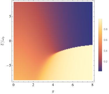
Figure 7: Left panel: Colour map of $\langle{S}_{z}^{2}\rangle$ obtained by the exact diagonalization. Right panel: Colour map of $\langle{S}_{z}^{2}\rangle$ obtained from the semiclassical solution, see main text. In both figures $\omega_{0}/\Delta=0.1$. The phase boundary predicted by the semiclassical approximation approaches the exact one in the quasi-thermodynamic limit $\omega_{0}/\Delta\to 0$.

III Optical conductivity in the ordered phase

The optical conductivity $\sigma(\omega)$ is a gauge-invariant observable. Here, we derive $\textrm{Re}[\sigma(\omega)]$ in the leading order in $\Delta$. This result is applicable deep in the ordered phase where $\langle S_{z}\rangle\approx S$, $\langle S_{z}\rangle$ is the ground-state average of the semiclassical Hamiltonian $H_{\text{sm}}$, and $S$ is the value of orbital pseudospin. Here, we assume $S\geq 1$, such that the dipole-dipole interaction $US_{z}^{2}$ is non-trivial. Indeed, in this case effects of the “depolarization” field $-\Delta S_{x}$ are weak and therefore, they can be treated via the perturbation theory. Note that the light-matter coupling constant $g$ can be of arbitrary value and the perturbation expansion is performed only in the small parameter $\Delta/|US|$. It is more convenient to present the derivation within the Peierls gauge, see Eq. (2) in the main text. The current operator $J$ along the DQD axis $z$ follows from the fact that the coordinate operator is given by $z=bS_{z}$ in the Peierls gauge, where $b$ is the separation between left and right minima within each DQD:

$$J=e\frac{dz}{dt}=i\left[H,ebS_{z}\right]=i\frac{eb\Delta}{2}\left(e^{g(a-a^{\dagger})}S_{+}-e^{-g(a-a^{\dagger})}S_{-}\right).$$ (18)

First, we calculate the current-current correlator $\Pi(g,t)$,

$$\Pi(g,t)=-i\theta(t)\Bigl{\langle}\left[J^{H}(t),J(0)\right]\Bigr{\rangle},$$ (19)

where $J^{H}(t)=e^{iHt}Je^{-iHt}$ is the Heisenberg representation of the current operator and $\theta(t)$ the Heaviside step function. Within leading order in $\Delta$, $\Pi(g,t)$ is given by the following average:

$$\Pi_{0}(g,t)=-i\theta(t)\Bigl{\langle}\left[J(t),J(0)\right]\Bigr{\rangle},$$ (20)

where $J(t)=e^{iH_{0}t}{J}e^{-iH_{0}t}$ is the interaction representation of the current operator, $H_{0}$ is given by Eq. (1) in the main text. First we note that $S_{z}(t)=S_{z}$ as $[H_{0},S_{z}]=0$. The interaction representations of $S_{+}$ and $a$ are the following:

$$S_{+}(t)=e^{-iK(S_{z})t}S_{+}=S_{+}e^{-iK(S_{z}+1)t},$$ (21)

$$a(t)=e^{-i\omega_{0}t}a,$$ (22)

where $K(S_{z})=H_{0}(S_{z}-1)-H_{0}(S_{z})=V_{b}+U(1-2S_{z})$. The statistical average of the exponential operators then follows directly from the Campbell-Baker-Hausdorff formula,

$$F(g,t)\equiv\Bigl{\langle}e^{g({a}(t)-{a}^{\dagger}(t))}e^{-g({a}-{a}^{\dagger})}\Bigr{\rangle}=e^{-g^{2}\left(2N_{\text{ph}}+1\right)}\exp\left[2g^{2}N_{\text{ph}}\cos(\omega_{0}t)+g^{2}e^{-i\omega_{0}t}\right],$$ (23)

where $N_{\text{ph}}=[e^{\beta\omega_{0}}-1]^{-1}$ is the average photon number at finite temperature $T=1/\beta$. As $\langle{S}_{+}(t){S}_{+}\rangle=\langle{S}_{-}(t){S}_{-}\rangle=0$, we find

$$\Pi_{0}(g,t)=F(g,t)\Pi_{0}(g=0,t),$$ (24)

where $\Pi_{0}(g=0,t)$ is the current-current correlator of the electron system decoupled from photons. We emphasize that the factorization in Eq. (24) holds in the limit $\Delta\ll\langle K({S}_{z})\rangle$, i.e. when the hopping $\Delta$ can be treated as a small perturbation. In the limit $\Delta=0$, $H=H_{0}$, see Eq. (1) in the main text, and the ground state at $U<0$ is the state with the maximal spin projection ($S_{z}=S$ at $V_{b}>0$ and $S_{z}=-S$ at $V_{b}<0$),

$$\Pi_{0}(g=0,t)=-i\theta(t)\frac{S}{2}\left(eb\Delta\right)^{2}e^{-itE_{\text{opt}}},$$ (25)

where $E_{\text{opt}}=|U|(2S-1)+|V_{b}|$ corresponds to the energy difference between the ground state and the first excited state of $\langle 0|H_{0}|0\rangle$ at $\Delta\to 0$, $|0\rangle$ is the photon vacuum. In order to see optical transitions between the ground state and the second excited state of $\langle 0|H_{0}|0\rangle$, two virtual spin flips are required, such transitions emerge in order $\propto\Delta^{4}$. We indeed observe such transitions in exact diagonalization, they are strongly suppressed compared to the leading harmonic, see Fig. 5 in the main text. In order to find the Fourier transform $\Pi_{0}(g,\omega)$, we use the Bessel function expansion,

$$e^{z\cos(\omega_{0}t)}=\sum\limits_{-\infty}^{\infty}I_{m}(z)e^{im\omega_{0}t},$$ (26)

where $I_{-m}(z)=I_{m}(z)$ is the modified Bessel function of the first kind. The real part of the optical conductivity then follows from Eq. (24),

$${\rm Re}\left[\sigma(\omega)\right]\approx-\frac{1}{\omega}{\rm Im}\left[\Pi_{0}(g,\omega)\right]=\frac{\pi S}{2\omega}\left(eb\Delta\right)^{2}\sum\limits_{n=0}^{\infty}p_{n}\left(g^{2}\right)\sum\limits_{m\in\mathbb{Z}}e^{-2g^{2}N_{\text{ph}}}I_{m}\left(2g^{2}N_{\text{ph}}\right)\delta\left(\omega-E_{\text{opt}}-(n-m)\omega_{0}\right),$$ (27)

where $\mathbb{Z}$ is the set of integers and $p_{n}(z)=e^{-z}z^{n}/n!$ the Poisson distribution. Notice that at $T=0$ we get $N_{\text{ph}}=0$, so only the $m=0$ term in Eq. (27) contributes, and we restore Eq. (12) in the main text.

The subleading $\propto\Delta^{4}$ harmonics can be calculated similarly via perturbative expansion with respect to the terms $\propto\Delta$ in $H$, see Eq. (2) in the main text. Here we only present the brightest harmonics $\propto\Delta^{2}$.