Bitrate Ladder Prediction Methods for Adaptive Video Streaming: A Review and Benchmark

Abstract

HTTP adaptive streaming (HAS) has emerged as a widely adopted approach for over-the-top (OTT) video streaming services, due to its ability to deliver a seamless streaming experience. A key component of HAS is the bitrate ladder, which provides the encoding parameters (e.g., bitrate-resolution pairs) to encode the source video. The representations in the bitrate ladder allow the client’s player to dynamically adjust the quality of the video stream based on network conditions by selecting the most appropriate representation from the bitrate ladder. The most straightforward and lowest complexity approach involves using a fixed bitrate ladder for all videos, consisting of pre-determined bitrate-resolution pairs known as “one-size-fits-all.” Conversely, the most reliable technique relies on intensively encoding all resolutions over a wide range of bitrates to build the convex hull, thereby optimizing the bitrate ladder for each specific video. Several techniques have been proposed to predict content-based ladders without performing a costly exhaustive search encoding. This paper provides a comprehensive review of various methods, including both conventional and learning-based approaches. Furthermore, we conduct a benchmark study focusing exclusively on various learning-based approaches for predicting content-optimized bitrate ladders across multiple codec settings. The considered methods are evaluated on our proposed large-scale dataset, which includes 300 UHD video shots encoded with software and hardware encoders using three state-of-the-art encoders, including AVC/H.264, HEVC/H.265, and VVC/H.266, at various bitrate points. Our analysis provides baseline methods and insights, which will be valuable for future research in the field of bitrate ladder prediction. The source code of the proposed benchmark and the dataset will be made publicly available upon acceptance of the paper.

I Introduction

In recent years, video streaming services such as video on demand (VOD) and live streaming have contributed significantly to Internet traffic. According to the Sandvine report [1], in the first half of 2022, video streaming accounted for 65.93% of overall Internet traffic. As a result, video service providers have invested considerable resources in optimizing the video encoding process to improve the quality of experience (QoE) and maintain seamless video streaming performance for all users.

HAS stands as the state-of-the-art video streaming technology, designed to guarantee the delivery of the highest possible visual quality at the target bitrate. In HAS, the video content is first split into short chunks, called segments, typically ranging from 2 to 10 seconds. These segments are pre-encoded at various resolutions and quality levels to accommodate a wide range of network conditions, device displays, and computing capabilities. The video segments stored on the server side are transmitted over HTTP to client devices based on their adaptive bitrate (ABR) algorithm [2] requests, which consider their specific bandwidth, display resolution, and computing resource requirements. To facilitate the bitrate selection process for each segment, a bitrate ladder is commonly utilized. The bitrate ladder consists of a set of encoding parameters, often referred to as bitrate-resolution pairs, which indicate the encoding configuration for each video segment. These pairs are organized hierarchically, with higher bitrates associated with higher video quality and resolutions. The primary objective of the bitrate ladder is to provide multiple representations of the video content, enabling client devices to dynamically select the representation that offers the highest possible quality. This adaptive selection process enhances reliability, minimizes buffering, and ultimately enhances the overall user experience.

One of the classical approaches to constructing a bitrate ladder is to use a static ladder. In this approach, usually referred to as one-size-fits-all bitrate ladder, a fixed set of encoding parameters, such as bitrate-resolution pairs, is recommended for all video contents regardless of their characteristics. Although this approach is easy to implement and provides a straightforward solution, it often fails to capture the characteristics and complexities of each video. This lack of granularity could lead to suboptimal streaming experiences, with some videos being transmitted at unnecessarily high bitrates, leading to bandwidth wastage. In contrast, other videos might suffer from poor quality and coding artifacts due to insufficient bitrate allocation. As a result, more adaptive and content-aware solutions have been proposed. For example, the per-title encoding solution introduced by Netflix [3] is a content-aware approach that individually encodes each source title, which is a specific piece of content such as a movie or a TV show, at various bitrates and resolutions, enabling the construction of its rate-distortion (RD) curves based on a perceptual quality metric. Fig. 1 illustrates RD curves of one video title using the video multi-method assessment fusion (VMAF) [4] quality metric. Subsequently, the Pareto-optimal points on these curves are identified, forming the convex hull. Bitrate-resolution pairs are then selected from the convex hull to define the bitrate ladder for each title. Later, this approach was further refined using per-shot encoding [5]. It involves segmenting each video into shots of similar frames that behave similarly when varying encoding parameters. This allows for determining a specific bitrate ladder for each shot, refining the adaptive convex hull approach, and enhancing the overall streaming experience. However, generating convex hulls for adaptive streaming, whether per video shot or title, is quite expensive due to the extensive space of encoding parameters, including resolution, quality level, codec type, etc. For example, determining the convex hull from sets of $R$ resolutions, $Q$ quality levels, and $C$ codecs, for a per-codec video content requires $R\times Q\times C$ encodings. This complexity results in a time-consuming and resource-intensive process, making it highly costly to VOD streaming and not suitable for live streaming.

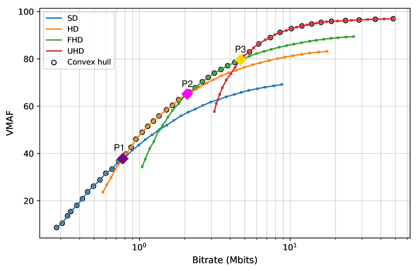
Figure 1: Example of rate-distortion curves and their convex hull for the sequence of India-scene-18 from the proposed dataset. P1, P2, and P3 denote the intersection points between SD-HD, HD-FHD, and FHD-UHD resolutions, respectively.

To address these challenges, numerous machine learning (ML)-based bitrate ladder prediction techniques have been proposed by both academic and industry experts in recent years [6, 7, 8, 9, 10, 11, 12, 13, 14, 15, 16]. These techniques aim to predict per-scene or per-shot bitrate ladders, eliminating the need for exhaustive encoding. In this context, we have conducted a benchmark study that compares various handcrafted- and deep learning (DL)-based methods, providing an in-depth analysis of their complexity and prediction performance. In addition, our benchmark incorporates a multi-codec approach to enhance the evaluation, allowing for a more comprehensive assessment of methods under different encoding scenarios. This comparison and analysis will contribute to a better understanding of the strengths and weaknesses of handcrafted (i.e., conventional) and DL techniques, ultimately guiding the development and comparison of more efficient and adaptable video streaming solutions. The principal contributions of this paper are listed as follows:

• A systematic classification and extensive review of current bitrate ladder construction methods for adaptive video streaming, including a detailed analysis of conventional and learning-based techniques.

• A large dataset with 300 Ultra-HD video sequences, encoded through hardware and software video encoders using three standards: AVC/H.264 [17], HEVC/H.265 [18], and VVC/H.266 [19] in four resolutions and multiple quantization parameter (QP) values.

• Exploring several handcrafted and DL-based features for both VOD and live streaming scenarios with various ML models for bitrate ladder prediction.

• A comprehensive benchmark study to assess the performance of ML-based methods, along with an in-depth analysis of prediction performance and complexity overhead on CPU and GPU platforms.

The remainder of this paper is organized as follows. Section II gives a comprehensive review of bitrate ladder prediction methods. Furthermore, the proposed dataset is presented and characterized in Section II. Section IV presents the development of benchmarking evaluation, while Section V provides and analyses the experimental results. Finally, Section VI concludes this paper.

II Bitrate ladder prediction methods

This section aims to provide a systematic classification and a comprehensive review of the existing methods for constructing bitrate ladders for adaptive video streaming. Specifically, we categorize these methods into two overarching categories: (i) conventional (i.e., do not involve any learning process) and (ii) learning-based. Furthermore, we subdivide the conventional techniques into static and dynamic methods, and the learning-based techniques are classified into handcrafted feature extraction methods and deep feature extraction based on deep neural networks, as depicted in Fig. 2.

II-A Conventional methods

II-A1 Static methods

The static (i.e., content-independent) bitrate ladder, also known as the one-size-fits-all bitrate ladder, is the conventional approach that offers predefined recommendations for encoding parameters, such as bitrate and resolution, for a given video content. Apple proposed one commonly adopted static bitrate ladder in Tech Note TN2224 [20]. Similarly, other video streaming platforms, such as YouTube [21] and Twitch [22], have also provided their own recommendations on encoding settings for their streamers. Although these one-size-fits-all bitrate ladders are simple to implement and straightforward to use, they have limitations in providing optimal encoding parameters for different types of videos. For complex videos, such as those with high-motion scenes, these static ladders may allocate insufficient bitrate, resulting in significant blocking and other visual artifacts. On the other hand, for less complex video content, such as cartoons, these ladders might over-allocate bitrate, leading to storage and bandwidth wastage. For instance, in Fig. 3, we plotted the RD curves of 50 video sequences at 1080p resolution encoded using the x265 software encoder at the same range of QP values. It demonstrates that some sequences reach very high Y-peak signal-to-noise ratio (YPSNR) (45 dB or more) at a bitrate of 1 Mbps or less. Conversely, some video sequences require bitrates of 20 Mbps or more to achieve a good YPSNR of 38 dB. Considering the diversity of video content, it is clear that a static scheme cannot provide the best video quality for a given title. This is why more advanced techniques have been proposed to address this limitation and improve the overall video streaming experience.

forked edges, for tree=draw,align=center,edge=-latex,fill=white,blur shadow, where level=1 for descendants=grow’=0, folder, l sep’+=-1pt, , [Bitrate ladder construction methods [Conventional methods [Static methods [Apple [20]] [YouTube [21]] [Twitch [22]] ] [Dynamic methods [Netflix [3, 23, 5]] [Chen et al. [24]] [Tashtarian et al. [25]] [Amirpour et al. [26]] [Reznik et al. [27, 28]] ] ] [Learning-based methods [Handcrafted feature-based methods [Goswami et al. [6]] [Bhat et al. [7]] [Takeuchi et al. [8]] [Katsenou et al. [9, 10]] [Silhavy et al. [11]] [Nasiri et al. [12]] [Menon et al. [13]] ] [Deep feature-based methods [Tianchi et al. [14]] [Xing et al. [29]] [Paul et al. [30]] [Amirpour et al. [31]] ] ] ]

Figure 2: Categories of bitrate ladder construction methods.

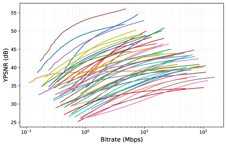
Figure 3: rd curves for 50 randomly sampled footage at 1080p resolution.

II-A2 Dynamic methods

At each resolution, the encoding quality improves with increasing bitrate, but there is a threshold beyond which the quality improvement becomes marginal. In the realm of dynamic methods, i.e., content-dependent, a per-title approach was first proposed by Netflix [3]. The primary task of this method is to encode the entire video at different quality levels and resolutions to build the convex hull of the RD curves based on the VMAF metric. Netflix’s per-title method uses this convex hull of the RD curves to create a customized bitrate ladder, tailored explicitly to the video’s content and characteristics, ensuring an improved QoE for viewers compared to static approaches. Later, as the Netflix service grew, they introduced an optimized per-chunk cloud-based encoding method [23] to enhance the scalability and reliability at a large scale. This approach identifies the most suitable bitrate-resolution pairs for all video chunks by evaluating their visual complexity through a constant rate factor (CRF)-based multi-pass encoding process. Nevertheless, both methods are suboptimal, as a title and even a chunk can contain various scenes with differing visual complexities. To address this shortcoming, Netflix’s research team proposed an optimized version of their method [5]. In this refined approach, a video is first divided into shots, which consist of adjacent frames that exhibit similar behavior when encoding parameters are altered. Each shot is then processed separately using the same exhaustive encoding approach as the original method to construct a per-shot bitrate ladder.

Similar to the approach in [5], the authors of [24] extracted the RD characteristics by conducting multiple encodes of each video chunk at various resolutions and bitrates. However, in contrast to the Netflix method, which primarily concentrates on content-based bitrate selection and the selection of rate-quality pairs located near the convex hull, the authors of this study also consider users’ bandwidth and the distribution of viewport sizes for the players.

Furthermore, Reznik et al. [27] introduced an analytical approach that takes into account both content behavior and network statistics when constructing the bitrate ladder. They frame the construction of the bitrate ladder as a non-linear constrained optimization problem, employing structural similarity index measure (SSIM)[32] as the quality metric and establishing bitrate constraints using probabilistic models. This approach was later extended to accommodate multiple codec types, including advanced video coding (AVC)/H.264 and high-efficiency video coding (HEVC)/H.265 [28]. Tashtarian et al. [25] developed LALISA, an online lightweight bitrate ladder optimization framework for HTTP-based live video streaming. LALISA dynamically determines the optimal bitrate ladder to achieve low encoding and delivery costs while maintaining an acceptable quality of experience during live sessions. Further, Amirpour et al. [26] proposed the per-title encoding using spatio-temporal resolutions (PSTR) method, which introduces the temporal resolution, specifically framerate, as an additional dimension to enhance the bitrate ladder prediction. This technique involves encoding each video chunk at multiple resolutions and framerates to identify the optimal settings at each bitrate. While the inclusion of temporal resolution in per-title encoding increases complexity, considering both resolutions results in higher bitrate savings.

II-B Learning-based methods

Learning-based methods refer to techniques that utilize machine learning methodologies to discern patterns and relationships from input video data for the purpose of generating a content-dependent bitrate ladder. These methods can be broadly classified into two categories based on whether they employ handcrafted or deep learning approaches to extract features from the video content.

II-B1 Handcrafted features

In learning-based methods, the first class focuses on approaches that leverage handcrafted features. These features are meticulously designed and manually derived from the video content to model and predict the optimal bitrate ladder for video encoding. For instance, Goswami et al. [6] introduced a method that combines exhaustive encoding with machine learning techniques to expedite the encoding process. In this approach, the video sequence initially undergoes encoding at a lower resolution. Subsequently, encoder decisions, including motion vectors, quad-tree structures for coding unit (CU), and predictions for prediction unit (PU), serve as handcrafted features. These features are harnessed to train a maximum a posteriori (MAP) classifier. This classifier, in turn, refines the encoder’s decision during higher-resolution encoding, resulting in a significant reduction in computational complexity. Bhat et al. [7] introduced an innovative approach to swiftly predict adaptive spatial resolutions without the need for multiple encodings. Their algorithm incorporates an extensive array of features, covering rate control-based factors (QP, frame rate, targeted bitrate), spatial features (histogram of pixel values, variance of coding tree unit (CTU)), temporal features (motion vectors (MVs), scene change scores), and encoder pre-analysis-based features (estimated QP of all frames in the initial group of pictures (GOP), estimated intra probability). A total of 43 input values are derived from various statistics extracted from these diverse features. Subsequently, these multifaceted features, together with their corresponding statistics, serve as inputs for a machine-learning classification model. The research indicates that both multilayer perceptron (MLP) and random forest (RF) classifiers are well-suited for this classification task.

In [8], the authors proposed a perceptual quality-driven method to generate an adaptive encoding recipe (i.e., adaptive encoding ladder). They employed the just noticeable difference (JND) scale to measure perceptual quality, which represents the smallest perceivable difference in visual quality that a human viewer can detect. The process begins with pre-encoding target sequences using fixed QPs at different resolutions and then extracting features such as bitrates, peak signal-to-noise ratio (PSNR), SSIM, and VMAF. These features are then used to estimate JND scores through support vector regression (SVR) estimation. This estimation process allows for optimizing the encoding recipe, ensuring that the differences in visual quality between successive encodings are perceptually noticeable to viewers. The objective is to improve storage size by reducing redundancies in perceptual quality, while still maintaining an acceptable level of visual experience. Menon et al. [13] similarly proposed a perceptually-aware online per-title encoding (PPTE) scheme for live streaming applications. ppte includes an algorithm that predicts the optimal bitrate-resolution pairs for every video segment based on JND. Specifically, ppte utilizes low-complexity discrete cosine transform (DCT)-energy-based features to assess video segments’ spatial and temporal complexity, enabling the prediction of bitrates where JNDs are located.

Moreover, Katsenou et al. [9] introduced a content-agnostic approach that harnesses machine learning, specifically Gaussian processes regression (GPR), to predict cross-over QPs for various spatial resolutions. These parameters determine the bitrates at which the switch between spatial resolutions should occur when encoding with the HEVC encoder. The authors employ GPR with rational quadratic kernels and incorporate handcrafted spatiotemporal features, such as gray level co-occurrence matrix (GLCM) and temporal coherence (TC), extracted from uncompressed ultra high definition (UHD) video sequences in their native resolutions to predict the cross-over QP values based on the YPSNR metric. In their subsequent work, Katsenou et al. [10] extended their approach to include the VMAF metric as an additional quality criterion. In a similar vein to [9], Silhavy et al. [11] leverage various machine learning algorithms, including SVR, MLP, and random forest regression (RFR), to construct a content-aware bitrate ladder based on VMAF as a quality metric.

An additional handcrafted feature-based method was introduced in [12]. This approach employs two supervised machine learning algorithms, a regression, and a classification method, trained on spatiotemporal features (GLCM, TC) extracted from uncompressed video sequences. An ensemble aggregation technique is applied to predict a bitrate ladder for the versatile video coding (VVC) encoder, improving the performance of both ML algorithms.

Lastly, Menon et al. [13] present a perceptually-aware bitrate ladder prediction approach that leverages DCT-energy-based low-complexity spatial and temporal features extracted from video sequence, as well as a newly introduced feature that combines the DCT-based features with the target bitrate of encoding. The method employs linear regression to predict the VMAF value corresponding to a resolution and target bitrate based on the extracted features.

II-B2 Deep features

In contrast to learning-based methods relying on handcrafted features, the deep-features category includes methods that leverage deep neural networks to extract relevant features from the video content. For instance, Tianchi et al. [14] introduced a reinforcement learning-based method called DeepLadder, which considers video content, network traffic capacity, and storage costs to estimate a suitable encoder setting for each resolution. The latter is mainly based on pre-trained ResNet-50 as the backbone model to extract spatial features from intra-frames.

Moving on, the authors in [29] proposed a content-adaptive rate control solution that utilizes a temporal segment network (TSN) [33] to extract spatiotemporal features from video content. The extracted features feed a fully connected (FC) layer followed by a Softmax function to predict the optimal rate-control target based on the content characteristics. This deep learning model supports both the average bitrate control and the CRF modes. The model learns to predict the optimal bitrate for the target rate control in the average bitrate mode. On the other hand, in the CRF mode, the model learns to predict the rate factor as the target.

Another DNN method is presented in [30], which employs a recurrent convolutional network (RCN) to estimate the convex hull of the video shots. This method jointly processes spatial and temporal information using convolutional gated recurrent units (Conv-GRUs) [34] to effectively capture long-term spatiotemporal properties throughout video shots. The prediction task is formulated as a multi-label classification problem rather than a regression problem. A transfer learning technique is employed to overcome the limited availability of uncompressed public video datasets for deep model training.

Moreover, Amirpour et al. [31] proposed a scalable content-aware per-title encoding system called DeepStream, designed to support CPU-only and GPU-available end-users. The proposed approach consists of two main layers: the base layer, which constructs a bitrate ladder based on any existing per-title encoding method, and the enhancement layer, which enhances QoE by incorporating content-aware deep video super-resolution using lightweight context-adaptive binary arithmetic coding for DNN compression. The system maintains backward compatibility for CPU-only end-users while providing improved perceived video quality for GPU-available end-users through lightweight content-aware video super-resolution DNNs and efficient DNN compression methods.

As many learning-based solutions necessitate large-scale datasets, our next section is dedicated to the construction of such a dataset. We will elaborate on our process for creating a comprehensive large-scale dataset to support the objectives of our study.

III Dataset construction

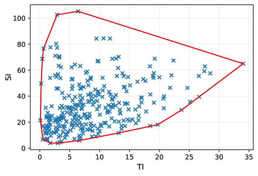
(a) SI vs. TI

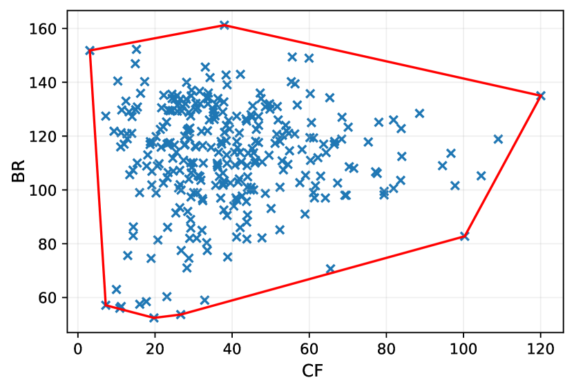
(b) BR vs. CF

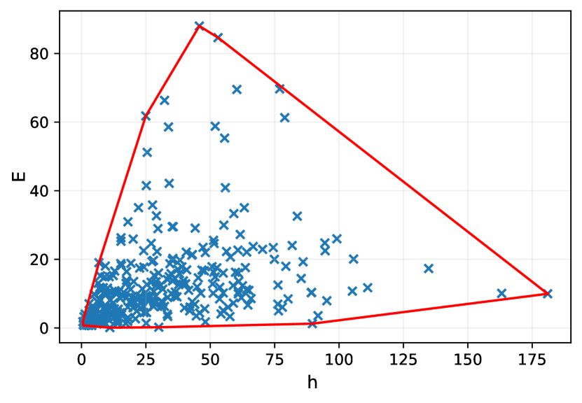
(b) h vs. E

Figure 4: Source content distribution in paired feature space with corresponding convex hulls. Left column: TI×SI, middle column: CF×BR and right column: hxE.

For any data-driven approach, the presence of a diverse and extensive video dataset that encompasses a wide array of scenes is indispensable. Thus, in this section, we present the adaptive video streaming dataset (AVSD), a comprehensive and diversified dataset containing 300 UHD video shots sourced from publicly available video sequences. Additionally, we provide the computed convex hulls for these shots, following encoding using three distinct video coding standards: AVC/H.264, HEVC/H.265, and VVC/H.266. We firmly believe that the availability of the AVSD dataset will be of immense value and contribute to the advancement of research in adaptive video streaming and related domains.

III-A Video collection

Researchers in the field of learned video compression often encounter a significant challenge: the scarcity of high-quality video content that is both an uncompressed (pristine) and publicly accessible. To address this limitation, we have meticulously curated a dataset comprising 300 videos. This dataset encompasses both pristine, uncompressed video sequences and high-quality compressed versions. Within this collection, we have assembled 120 pristine, uncompressed video sequences from a variety of sources, including Netflix Chimera [35], AWS Elemental [36], MCML [37], Harmonic [38], Ultra Video Group [39], SJTU [40], and the Waterloo IVC 4K Video Quality Database [41]. The remaining 180 sequences were thoughtfully selected from the YouTube-UGC dataset [42], exclusively featuring high-quality content. While many of these sequences initially boasted a resolution of 4096$\times$2160, they were subsequently cropped to 3840$\times$2160 and converted into a 4:2:0 chroma subsampled format, if not originally formatted as such. To ensure homogeneity, all sequences underwent a scene segmentation process, guaranteeing that each sequence comprises only a single scene. This segmentation was accomplished using the PySceneDetect tool [43]. As a final step, all sequences were temporally cropped to 64 frames, resulting in a dataset that offers a comprehensive view of different scenes and scenarios.

III-B Dataset characterization

Winkler et al. [44] originally proposed three video descriptors: spatial activity, temporal activity, and colorfulness, to characterize content diversity within datasets. In our study, we extend this analysis of content diversity by incorporating six low-level features. These features encompass spatial information (SI) [45], temporal information (TI) [45], brightness (BR) [46], colorfulness (CF) [46], and two novel features derived from video complexity analyzer (VCA) [47]: spatial complexity (E) and temporal complexity (h). Each of these features is computed individually for every frame in the dataset. Subsequently, the computed values are averaged to obtain an overall (mean) representation. To visualize the feature coverage of our dataset, we present scatter plots with convex hulls for paired features, as depicted in Fig. 4. It is evident that the video sequences in our dataset span a wide range of the spatiotemporal domain, with SI values ranging from 5 to 105 and TI values from 0 to 35. This diversity extends to the spatiotemporal complexities found within the dataset. The majority of videos exhibit low complexity, characterized by single-shot scenes. However, a smaller fraction contains highly complex shots, adding variety to the dataset. Additionally, the scatter plot of BR versus CF unveils a rich spectrum of content types. br values span from 60 to 160, indicating diverse lighting conditions and scene settings. Further, CF values range from 0 to 120, signifying a multitude of color palettes and visual styles.

III-C Convex hull construction

To determine the RD of video sequences and construct the ground truth bitrate ladder, we initiated the process by spatially downscaling all sequences. This downscaling was carried out using a Lanczos-3 filter [48] to create three different resolutions: full high definition (FHD), high definition (HD), and standard definition (SD). Subsequently, we encoded the video sequences in four resolutions, which included both the downsampled versions and the original UHD sequences, denoted as $\mathcal{S}\in\{3840\times 2160,1920\times 1080,1280\times 720,720\times 480\}$. These resolutions represent typical choices in streaming applications [49]. The encoding process was performed using three video coding standards: AVC/H.264, HEVC/H.265, and VVC/H.266. For the AVC/H.264 and HEVC/H.265 codecs, we employed both software and hardware-based implementations in random access (RA) configuration, using a range of constant QP values from $\mathcal{Q}\in\{15,16,\dots,44,45\}$. The encoding process for these codecs was conducted using FFmpeg [50]. Nevertheless, it is worth noting that as of now, there is no public hardware encoder implementation available for the VVC/H.266 standard. Thus, we solely utilized its software encoder, Fraunhofer versatile video encoder (VVenC) [51]. Similar to the other codecs, we operated the software encoder in random access configuration with a set of constant QP values from $\mathcal{Q}\prime\in\{16,18,\dots,46,48\}$. In total, this process resulted in the encoding of 564 different bitstreams for each source content, which amounted to a grand total of 169,200 encoded video shots. Further, it is essential to mention that the software encoding process was carried out on a 16-core Intel® Xeon W-2145 CPU running at a frequency of 3.70 GHz and equipped with 64 GB of RAM. On the other hand, for hardware encoding, we employed the NVIDIA GeForce RTX 2080 Ti graphics card. Following this, all the encoded bitstreams underwent a decoding process and were upsampled back to their original resolution (2160p) using the same filter. Subsequently, we proceeded to construct the RD curves. To do this, we measured the objective video quality of the decoded sequences using two full-reference quality metrics: Y-PSNR and VMAF. Finally, we defined the intersection points between the RD curves of the same video across different resolutions to create the convex hull. Specifically, we identified these points as SD-HD, HD-FHD, and FHD-UHD, denoted as P1, P2, and P3, respectively. These points are visually represented in Fig. 1 for a specific video shot encoded with the x.264 software encoder.

IV Benchmark description for bitrate ladder construction

This section describes our benchmark for evaluating learning-based methods for bitrate ladder construction in adaptive video streaming. Our benchmark is divided into two primary categories, focusing on distinct approaches to predicting optimal bitrate ladders: (i) methods based on handcrafted features and (ii) methods based on deep neural networks. By comparing the performance of these two categories of methods, our benchmark aims to offer valuable insights into their respective strengths and limitations, ultimately guiding researchers and practitioners toward more effective and efficient adaptive video streaming solutions.

IV-A Methods based on handcrafted features

This subsection presents the handcrafted feature-based methods to predict bitrate ladders in adaptive video streaming. We focus on two sets of handcrafted features. The initial set consists of classic low-level features successfully used in compression and video streaming-related research [9, 52, 53]. Although these classic features are widely used, their extraction can be computationally expensive and time-consuming, especially for UHD videos, making them more appropriate for VOD streaming applications, hence referred to as VoD-HandC features.

On the other hand, the VCA features, referred to as Live-HandC features in this context, aim to provide a more efficient alternative for live-streaming scenarios with real-time and low latency constraints. The results of these methods, including their complexity, will be further explored in Section V.

TABLE I: List of VoD-HandC features and their statistics.

Features Statistics Grey-Level Co-occurrence Matrix (GLCM) F1.$\textrm{meanGLCM}_{\textrm{cor}}$, F2.$\textrm{stdGLCM}_{\textrm{cor}}$, F3.$\textrm{meanGLCM}_{\textrm{con}}$, F4$\textrm{stdGLCM}_{\textrm{con}}$, F5.$\textrm{meanGLCM}_{\textrm{enr}}$, F6.$\textrm{stdGLCM}_{\textrm{enr}}$, F7.$\textrm{meanGLCM}_{\textrm{hom}}$, F8.$\textrm{stdGLCM}_{\textrm{hom}}$, F9.$\textrm{meanGLCM}_{\textrm{ent}}$, F10.$\textrm{stdGLCM}_{\textrm{ent}}$ Temporal Coherence (TC) F11.$\textrm{meanTC}_{\textrm{mean}}$, F12.$\textrm{meanTC}_{\textrm{std}}$, F13.$\textrm{stdTC}_{\textrm{mean}}$, F14.$\textrm{stdTC}_{\textrm{std}}$, F15.$\textrm{meanTC}_{\textrm{skw}}$, F16.$\textrm{stdTC}_{\textrm{skw}}$, F17.$\textrm{meanTC}_{\textrm{kur}}$, F18.$\textrm{stdTC}_{\textrm{kur}}$, F19.$\textrm{meanTC}_{\textrm{entr}}$, F20.$\textrm{stdTC}_{\textrm{entr}}$ Spatial Information (SI) F21.mean_SI, F22.std_SI Temporal Information (TI) F23.mean_TI, F24.std_TI Colorfulness (CF) F25.mean_CF, F26.std_CF Noise estimation F27.mean_Noise, F28.std_Noise Normalized Cross Correlation (NCC) F29.mean_NCC, F30.std_NCC

IV-A1 VoD-HandC features

identifying suitable spatiotemporal features that reflect the sequence content characteristics is essential, especially for building an efficient content-gnostic bitrate ladder. The VoD-HandC feature extraction process can be modulated as follows:

$$\mathcal{S}_{F_{i}}=\Psi_{\text{VoD}}(\mathcal{V}),$$ (1)

where $\mathcal{S}_{F_{i}}$ represents the extracted features set, the $\Psi_{\text{VoD}}$ represents VoD-HandC feature extraction module, while $\mathcal{V}$ denotes the input video sequence.
We have selected a set of spatiotemporal features from various low-level features successfully used in our previous related work [53]. The chosen features listed below effectively capture the content characteristics essential for constructing a content-aware bitrate ladder. Table I provides the full set of these features and their statistics.
glcm [54] is a spatial feature that characterizes the distribution of gray levels within an image by examining the contrast in intensity between adjacent pixels. By quantifying the occurrence frequency of pairs of pixel values at defined spatial relationships, such as distance and direction, GLCM offers valuable insights into the texture and patterns present in the image. GLCM comprises five fundamental descriptors: contrast, correlation, homogeneity, energy, and entropy.
tc [55] is a temporal feature employed to characterize the predictability of one frame based on its temporal predecessor. It assesses the consistency of spectral amplitude between two consecutive images, which, in turn, reflects the ease or complexity of the temporal prediction process. In practical terms, TC is computed for each pair of successive frames, and sequence-level statistics are derived, including mean, standard deviation, skewness, kurtosis, and entropy.
si [45] is a feature employed to gauge the level of spatial detail within an image, encompassing textures, patterns, and structures. SI quantifies the associations among pixel intensity values within an image, offering insights into local variations in the image. When analyzing SI across an entire video sequence, statistical measures like mean and standard deviation are computed, contributing to a holistic assessment of the sequence’s spatial characteristics.
ti [45] is a feature used to evaluate the video’s temporal characteristics, such as motion, scene changes, and object dynamics. TI quantifies the relationships between consecutive frames, offering insight into the changes and variations over time. To analyze TI across an entire video sequence, statistics such as mean and standard deviation are calculated, providing a comprehensive understanding of the temporal properties of the video sequence.
Colorfulness (CF) [46] is a spatial feature employed to evaluate the richness and diversity of colors within a picture. It quantifies the degree of color variation and saturation, offering insights into the visual appeal and vibrancy of the content. Analyzing CF across an entire video sequence requires computing statistics such as mean and standard deviation.
Noise estimation [56] is a spatial feature employed to evaluate the presence and intensity of noise within an image. It measures the extent of random variations, artifacts, or distortions in pixel values, providing insight into the overall quality and sharpness of the content. The mean and standard deviation are computed to analyze the noise estimation across the entire video sequence.
ncc [57] is a similarity measure used to assess temporal similarity between frames. The correlation of pixel intensity values between two successive frames indicates the degree of resemblance or motion between the frames. To analyze normalized cross correlation (NCC) across an entire sequence, the NCC is computed for each pair of consecutive frames, followed by the calculation of sequence-level statistics, such as mean and standard deviation.

TABLE II: List of Live-HandC features and their statistics.

Features	Statistics
Spatial energy (E)	F1.meanE, F2.stdE, F3.minE,
	F4.maxE, F5.$25^{th}$E, F6.$50^{th}$E,
	F7.$75^{th}$E, F8.iqrE, F9.skwE,
	F10.kurE
Temporal energy (h)	F11.meanh, F12.stdh, F13.minh,
	F14.maxh, F15.$25^{th}$h, F16.$50^{th}$h,
	F17.$75^{th}$h, F18.iqrh, F19.skwh,
	F20.kurh
Gradient of temporal energy ($\epsilon$)	F21.meanϵ, F22.stdϵ, F23.minϵ,
	F24.maxϵ, F25.$25^{th}$ϵ, F26.$50^{th}$ϵ,
	F27.$75^{th}$ϵ, F28.iqrϵ, F29.skwϵ
	F30.kurϵ
Brightness (BR)	F31.meanBR, F32.stdBR, F33.minBR,
	F34.maxBR, F35.$25^{th}$BR, F36.$50^{th}$BR,
	F37.$75^{th}$BR, F38.iqrBR, F39.skwBR,
	F40.kurBR

IV-A2 Live-HandC features

The VoD-HandC features have been extensively explored in the realms of computer vision and compression-related fields. However, their extraction process may prove to be relatively time-consuming, especially when dealing with high-resolution videos. This is primarily due to the lack of optimization for online analysis, which diminishes their suitability for real-time applications. In response to this issue, Menon et al. [47] have introduced an alternative solution known as VCA, which leverages low-complexity features. vca is tailored for online video content complexity analysis, ensuring low-latency video streaming and enhanced real-time performance. The extraction process for Live-HandC features can be defined as follows:

$$\mathcal{S}_{F_{i}}=\Psi_{\text{Live}}(\mathcal{V}),$$ (2)

Here, $\mathcal{S}_{F_{i}}$ represents the set of extracted features, $\Psi_{\text{Live}}$ corresponds to the Live-HandC feature extraction module, and $\mathcal{V}$ denotes the input video sequence. The VoD-HandC features are presented below.
Spatial energy (E) is used to quantify the complexity and variation of textures within an image. It is calculated using a DCT-based energy function that determines the block-wise texture of each frame.
Temporal energy (h) is a temporal feature that measures changes in texture complexity and variation between consecutive frames in a video sequence. The temporal energy is calculated through the sum of absolute differences (SAD) of the texture energy of each frame compared to its previous frame on a block-wise basis.
Gradient of temporal energy ($\epsilon$) is a feature that quantifies the rate of change in texture complexity and variation between consecutive frames in a video sequence. It is calculated as the ratio of the difference between temporal energy (h) values of the $(p-1)^{th}$ and $p^{th}$ frames with the h value of the $(p-1)^{th}$ frame.
Brightness (BR) is a spatial feature that quantifies the overall light intensity of a picture.

Finally, Table II provides the full set of listed features and their statistics. To provide a comprehensive understanding of the entire video, various statistics, such as mean, standard deviation, maximum, minimum, $25^{th}$ percentile, $50^{th}$ percentile, $75^{th}$ percentile, interquartile range (IQR), skewness and kurtosis are computed for each feature.

TABLE III: Selected features of predicted cross-over bitrates for RD curves based on YPSNR.

Cross-over bitrates	Codec	AVC		HEVC		VVC
	Plateform	Software (FFmpeg)	Hardware (NVENC)	Software (FFmpeg)	Hardware (NVENC)	Software (VVenC)
P3	VoD-HandC features	F5, F7, F11, F13, F26, F27, F29	F1, F5, F7, F11, F13, F17, F25-F27, F29	F3, F7, F11-F13, F29, F30, F27	F1, F5, F7, F11-F13, F17, F25-F27, F29	F7, F9, F11, F12, F13, F25, F27, F29
	Live-HandC features	F5, F11, F12, F13, F15, F16, F34, F39	F3, F12, F13, F15, F16, F19, F34	F5, F12, F13, F15, F18, F31, F33, F34, F38	F5, F12, F13, F15, F16, F19, F31, F35, F38	F1, F6, F10, F13, F15, F17, F19, F33, F34, F35-F39
P2	VoD-HandC features	F5, F7, F9-F13, F16, F25-F27, F29	F5, F7, F11, F13, F16, F25, F26, F27, F29	F7, F10, F11, F13, F19, F25, F27, F29	F1, F3, F5, F7- F9, F11-F13, F16, F25-F27, F29, F30	F5, F7, F9-F13, F25, F27, F29
	Live-HandC features	F6, F11-F13, F15, F16, F18, F31, F33, F34, F37-F39	F5, F7, F11-F13, F15, F16, F18, F19, F31, F34, F38, F40	F3, F4, F6, F9, F11, F13, F15, F31, F34, F36, F37, F38, F40	F3, F5, F11-F17, F31, F35, F38, F39	F5, F9, F10, F11, F13, F15, F21, F29, F31, F32, F36, F38,F39
P1	VoD-HandC features	F3, F5-F7, F10-F13, F26, F27, F29	F5, F7, F8, F11, F13, F29	F1-F3, F5, F7, F8, F10-F14, F25, F27, F29	F1, F3, F5-F13, F16, F25-F27, F29, F30	F6-F14, F16, F19,F25, F29, F30
	Live-HandC features	F3, F4, F9-F11, F13, F15, F18, F19, F34, F38	F3-F5, F9, F10, F11, F13, F15, F16, F18, F19, F38, F40	F3, F5, F6, F10, F11, F13-F16, F18, F38	F1, F5, F12-F16, F35, F37, F38, F39	F5, F9, F10, F13, F18, F19, F26, F32, F38, F40

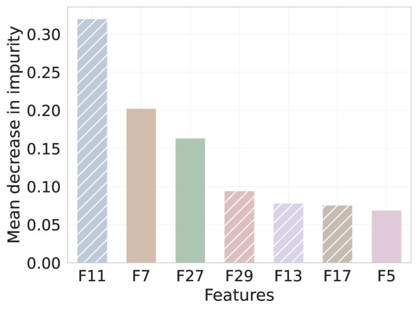
(a) VoD-HandC feature importance

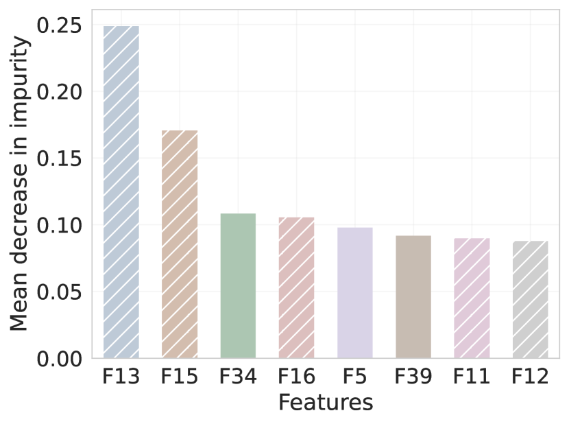
(b) Live-HandC feature importance

Figure 5: Feature importance of selected features for P3 cross-point prediction for x264 software encoding in terms of YPSNR. Dashed bars represent temporal features.

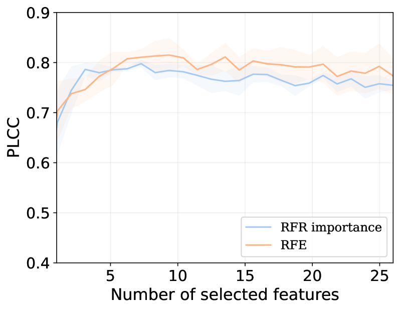
(a) VoD-HandC feature selection

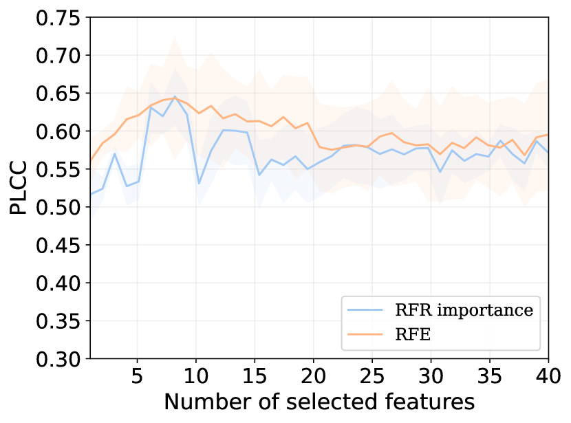
(b) Live-HandC feature selection

Figure 6: Feature selection performance (PLCC) for P3 cross-point prediction for x264 software encoding in terms of YPSNR. The shaded error bar represents the standard deviation of PLCC over 3 iterations.

IV-A3 Feature selection

In the context of increasing data dimensionality, the challenge of determining which features to incorporate into machine learning models has become paramount. Feature selection addresses this challenge by identifying the most pertinent and informative features within a dataset. This, in turn, bolsters machine learning models by reducing dimensionality, mitigating overfitting, and decreasing computational complexity. In our approach, we employ two types of feature selection algorithms to distill the initial feature set, denoted as $\mathcal{S}{F_{i}}$, into a refined feature set, referred to as $\mathcal{S}{F_{s}}$, for both VoD-HandC and Live-HandC features. This process ensures optimal model efficiency and accuracy. The first type of feature selection employs model-based feature selectors. In this category, we utilize the RFR algorithm known for its robustness and effectiveness in handling complex datasets. The RFR algorithm fits a regression model, capturing the relationships between features and the target variable. One key advantage of RFR-based feature selectors is their capacity to calculate the permutation importance of each feature, as illustrated in Fig. 5. By ranking the features based on their permutation importance, we can discern and eliminate the least significant ones. The second technique involves applying recursive feature elimination (RFE) to systematically remove the weakest features. The RFE operates by iteratively fitting a machine learning model, ranking features based on their importance, and subsequently eliminating the least important ones. In this study, we utilize ExtraTrees [58] as the target regressor. In the first step, we evaluated both of these feature selection methods on 3 test-training iterations using stratified sampling. Fig. 6 illustrates the median pearson linear correlation coefficient (PLCC) performance for P3 cross point prediction for x264 software encoding in terms of YPSNR. Following this comparison, we chose to proceed with the RFE technique due to its superior results. The resulting selected features for predicting cross-over bitrates are presented in Table III for YPSNR RD curves. Finally, these selected features are used to train a regression machine learning model for predicting the bitrate ladder, as outlined below:

$$\hat{P_{k}}=\theta_{k}(\mathcal{S}_{F_{s}}),$$ (3)

where $\hat{P_{k}}$ denotes the predicted value for $P_{k}$ on the bitrate ladder $P=(P_{1},P_{2},P_{3})$, $\theta_{k}$ is the parametric function of the regression ML model, while $\mathcal{S}_{F_{s}}=\{\text{F1},\dots\text{Fm}\}$ represents the selected feature set.

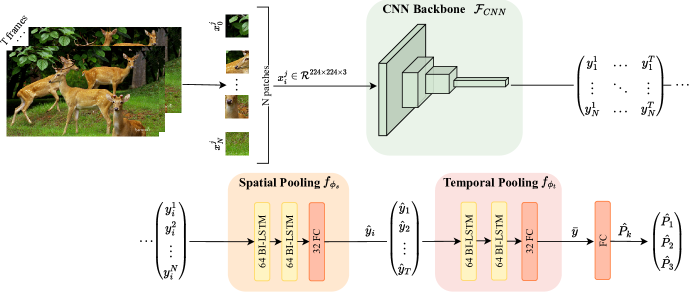
Figure 7: The overall framework of the proposed DNN methods. The feature extraction module is used to extract spatial features $\bm{y}_{i}^{j}$ from patches $\bm{x}_{i}^{j}$. The spatial and temporal pooling modules are used to aggregate features into a final vector $\bar{\bm{y}}$. Finally, the regression module uses the final vector $\bar{\bm{y}}$ to predict the cross-over bitrates $\hat{P_{k}}$.

IV-B Methods based on deep neural network

Recently, DNNs have gained tremendous attention in the field of computer vision due to their remarkable abilities to process complex visual data and solve a wide range of computer vision problems. In light of these advances, exploring the merit of using deep learning techniques to construct a content-gnostic bitrate ladder in the adaptive video streaming field is well-deserved. Thus, we investigate the application of DNN to achieve this goal in this subsection. As illustrated in Fig. 7, the proposed DNN solution’s framework consists of four main modules: feature extraction, spatial pooling, temporal pooling, and bitrate ladder regression module.

IV-B1 Feature extraction

Compared to traditional ML-based methods, deep convolutional neural network (CNN) features provide a more powerful approach to modeling complex data. By automatically learning and hierarchically representing local features, deep CNNs enable the network to extract higher-level abstractions from raw input video shots. However, the efficacy of CNNs is closely tied to the amount of training data available, and the proposed dataset is still much smaller than the typical computer vision datasets with millions of samples. To overcome this limitation, we used pre-trained models on the extensive ImageNet dataset [59] as backbone models, serving as deep feature descriptors. By employing these pre-trained models, we can leverage the knowledge learned from the vast amount of training data in ImageNet, significantly enhancing the feature representation and overall performance of DNN approaches in the context of bitrate ladder prediction.

When using pre-trained models, one challenge is dealing with their fixed input shape requirements. Two potential alternative solutions to address this constraint are resizing the input frame or dividing it into multiple patches. However, the first method could adversely lead to a loss of fine-grained details and introduce distortions, which may affect the network’s ability to extract meaningful features for the accurate prediction of bitrate-resolution pairs. Consequently, we chose the second approach.

Let us consider the input sequence $\mathcal{V}$ as a set of $T$ consecutive frames: $\mathcal{V}=\{\bm{x}_{1},\bm{x}_{2},\dots,\bm{x}_{T}\}$. For each frame $\bm{x}_{i}$ a sliding window is used to extract $N$ non-overlapping patches $\bm{x}_{i}^{j}$ of size $224\times 224$, where $j\in\{1,\dots,N\}$ and $i\in\{1,\dots,T\}$. Then, these patches $\bm{x}_{i}^{j}$ are fed into the CNN backbone pre-trained on ImageNet [59] for the extraction of spatial features $\bm{y}_{i}^{j}$ expressed as follows:

$$\bm{y}_{i}^{j}=\mathcal{F}_{CNN}(\bm{x}_{i}^{j}).$$ (4)

where $\mathcal{F}_{CNN}$ denotes the CNN backbone.

IV-B2 Spatial pooling

Once the features have been extracted from each patch, it is necessary to aggregate them into one vector per frame. This vector effectively encapsulates the spatial information of the frame, summarizing the distinct features of individual patches into a comprehensive representation. Traditionally, this is done using a spatial pooling technique. However, since patches within a frame are correlated and can be treated as a sequence, we employ an bi-directional long short term memory (Bi-LSTM) network to process the patch features sequentially in both directions. This allows Bi-LSTM to capture dependencies across the sequence of patches, reflecting their spatial relationships. Thus, the Bi-LSTM serves as a form of spatial pooling, effectively summarizing local features while reducing computational complexity and efficiently capturing short-term dependencies between neighboring patches.

The module is composed of two Bi-LSTM layers followed by a FC layer with 256 nodes. We have found that using this architecture leads to the best results in our experiments. The feature vector $(\bm{y}_{i}^{1},\bm{y}_{i}^{2},\dots,\bm{y}_{i}^{N})^{T}$ of a frame $i$ is fed into the spatial pooling module, expressed as:

$$\hat{\bm{y}}_{i}=f_{\phi_{s}}(\bm{y}_{i}^{1},\bm{y}_{i}^{2},\dots,\bm{y}_{i}^{N}),\hskip 8.53581pt\forall i\in\{1,\dots,T\},$$ (5)

where $f_{\phi_{s}}$ is the parametric function of the spatial pooling module with the training parameters $\phi_{s}$.

TABLE IV: Performance comparison in YPSNR / VMAF of the considered models on the proposed dataset with AVC encoder. The top result for each encoder type is highlighted in boldface.

Encoder type		AVC software encoding
Model \ Metric		R2 $\uparrow$	SROCC $\uparrow$	PLCC $\uparrow$	Accuracy $\uparrow$	BD-BR vs EEL $\downarrow$	BD-BR vs SL $\downarrow$
VoD-HandC	ExtraTrees	0.7265 / 0.5559	0.7466 / 0.7252	0.8689 / 0.7741	0.8462 / 0.8056	2.529% / 4.193%	-6.785% / -7.965%
	Random Forests	0.6760 / 0.5360	0.7114 / 0.6984	0.8308 / 0.7751	0.8309 / 0.7932	2.655% / 4.229%	-6.852% / -7.454%
	XGBoost	0.6629 / 0.5385	0.7263 / 0.6418	0.8241 / 0.6241	0.8395 / 0.7984	2.749% / 4.326%	-6.893% / -7.863%
	LightGBM	0.6143 / 0.5192	0.6472 / 0.6318	0.7925 / 0.7341	0.8235 / 0.8086	2.850% / 4.465%	-5.719% / -6.457%
Live-HandC	ExtraTrees	0.3854 / 0.2869	0.6885 / 0.6209	0.6347 / 0.5671	0.7980 / 0.7558	4.040% / 5.226%	-5.307% / -6.029%
	Random Forests	0.3325 / 0.2429	0.6629 / 0.6072	0.5788 / 0.4399	0.7977 / 0.7589	4.200% / 6.057%	-5.229% / -5.253%
	XGBoost	0.3395 / 0.2417	0.6700 / 0.5905	0.5864 / 0.4951	0.8009 / 0.7483	3.718% / 5.935%	-5.401% / -7.123%
	LightGBM	0.2729 / 0.1745	0.5993 / 0.5114	0.5338 / 0.4327	0.7831 / 0.7350	5.313% / 7.394%	-3.865% / -3.788%
Deep features	DensNet169	0.4964 / 0.5294	0.5487 / 0.6013	0.6813 / 0.7507	0.8032 / 0.7913	3.582% / 5.264%	-5.174% / -6.574%
	VGG16	0.5119 / 0.5133	0.5295 / 0.6000	0.7125 / 0.7373	0.7908 / 0.7845	3.368% / 7.966%	-5.165% / -6.637%
	ResNet-50	0.5416 / 0.5421	0.5371 / 0.6438	0.7425 / 0.7437	0.8155 / 0.7988	2.901% / 4.268%	-6.694% / -7.025%
	ConvNeXtBase	0.5381 / 0.5384	0.5544 / 0.5789	0.7323 / 0.7416	0.7982 / 0.7841	3.323% / 5.678%	-5.489% / -6.051%
Encoder type		AVC hardware encoding
Model \ Metric		R2 $\uparrow$	SROCC $\uparrow$	PLCC $\uparrow$	Accuracy $\uparrow$	BD-BR vs EEL $\downarrow$	BD-BR vs SL $\downarrow$
VoD-HandC	ExtraTrees	0.6461 / 0.4431	0.5994 / 0.5451	0.8200 / 0.6885	0.8075 / 0.7856	3.017% / 3.478%	-6.439% / -5.594%
	Random Forests	0.5749 / 0.3289	0.5568 / 0.5152	0.7824 / 0.6343	0.7958 / 0.7719	3.502% / 4.251%	-5.979% / -4.938%
	LightGBM	0.5591 / 0.4706	0.5097 / 0.4561	0.7752 / 0.6231	0.7871 / 0.7565	4.343% / 4.663%	-5.642% / -4.856%
	XGBoost	0.5117 / 0.3207	0.5391 / 0.4696	0.7385 / 0.6073	0.7849 / 0.7507	4.452% / 5.675%	-3.982% / -4.041%
Live-HandC	ExtraTrees	0.2943 / 0.2617	0.5092 / 0.4290	0.5787 / 0.5438	0.7622 / 0.7432	4.547% / 4.606%	-5.292% / -4.512%
	Random Forests	0.2733 / 0.3032	0.4975 / 0.4311	0.5451 / 0.5709	0.7540 / 0.7347	5.523% / 4.892%	-4.352% / -3.952%
	LightGBM	0.2560 / 0.2418	0.4647 / 0.3657	0.5124 / 0.5225	0.7589 / 0.7492	5.363% / 5.453%	-4.605% / -4.152%
	XGBoost	0.1997 / 0.1926	0.4075 / 0.3524	0.4784 / 0.4650	0.7543 / 0.7312	5.920% / 6.253%	-3.105% / -3.573%
Deep features	DensNet169	0.3875 / 0.3880	0.5986 / 0.5275	0.6550 / 0.6592	0.7890 / 0.7811	3.497% / 3.997%	-5.512% / -4.248%
	VGG16	0.4477 / 0.3849	0.6023 / 0.5095	0.6871 / 0.6431	0.7921 / 0.7663	3.678% / 3.999%	-5.041% / -3.812%
	ResNet-50	0.5534 / 0.4152	0.6048 / 0.5567	0.7042 / 0.6462	0.7940 / 0.7803	3.249% / 3.807%	-5.754% / -4.502%
	ConvNeXtBase	0.5116 / 0.4033	0.5601 / 0.4737	0.7022 / 0.6349	0.7967 / 0.7716	3.320% / 3.932%	-5.605% / -4.277%

IV-B3 Temporal pooling

parallel to the spatial aggregation process, temporal aggregation of frame features into a single vector per sequence is also a critical step. This temporal modeling module captures the dynamic changes and patterns over time, providing a critical dimension of information for predicting the bitrate ladder. Hence, we employ a temporal modeling module that utilizes a Bi-LSTM network to consolidate the frame-level features, denoted as $(\hat{\bm{y}}_{1},\hat{\bm{y}}_{2},\dots,\hat{\bm{y}}_{T})$ , into a comprehensive global feature vector $\bar{\bm{y}}$ that encapsulates the entire video sequence. bi-lstm networks are adept at considering both forward and backward information, enabling the capture of long-range dependencies among frames. Analogous to the spatial modeling, this module comprises two Bi-LSTM layers, each with 64 cells, and is subsequently followed by a FC layer containing 256 nodes. The temporal modeling module can be expressed as follows:

$$\bar{\bm{y}}=f_{\phi_{t}}(\hat{\bm{y}}_{1},\hat{\bm{y}}_{2},\dots,\hat{\bm{y}}_{T}),$$ (6)

where $f_{\phi_{t}}$ is the parametric function of the temporal modeling module with the training parameters $\phi_{t}$.

IV-B4 Bitrate ladder regression

Following the extraction and aggregation of deep features into a single representative vector $\bar{y}$, the challenge lies in mapping these features onto the respective point in the final bitrate ladder. To address this, we employed one node in a FC layer as a regression model with a linear activation function to predict a single point on the bitrate ladder. To predict the complete bitrate ladder, $P=(P_{1},P_{2},P_{3})$, we implemented three distinct models, each consisting of a spatial and temporal module as described above, followed by the regression module. We have found that using this architecture, with separate models for each point on the bitrate ladder, leads to the best results in our experiments. Consequently, the prediction for each point in the bitrate ladder can be formulated as follows:

$$\hat{P_{k}}=\zeta_{k}(\bar{\bm{y}}),$$ (7)

where $\hat{P_{k}}$ represents the predicted value for $P_{k}$ on the bitrate ladder $P=(P_{1},P_{2},P_{3})$ and $\zeta_{k}$ denotes the FC layer, where $k\in\{1,2,3\}$.

V Experimental results

In this section, we first define the experimental setup, including the baselines, the evaluation methods, and the implementation details. Then, we present the coding performance regarding the coding efficiency and complexity.

V-A Experimental setup

V-A1 Baselines

due to the lack of publicly available implementations for many of the methods discussed in Section II, we opted to benchmark the performance of our proposed models against two alternative methods. These methods, outlined below, offer a trade-off between computational cost, simplicity, and compression performance:

eel: this approach, based on exhaustive encoding detailed in Subsection III-C, provides a reference point for our performance measurements by generating a fully specialized bitrate ladder for each content. The exhaustive encoding ladder (EEL) approach also serves as the ground truth during the training stage.

sl: this method creates a fixed bitrate resolution pair by averaging the ground truth bitrate ladders obtained from the training dataset (using the EEL approach).

TABLE V: Performance comparison in YPSNR / VMAF of the considered models on the proposed dataset with HEVC encoder. The top result for each encoder type is highlighted in boldface.

Encoder type		HEVC software encoding
Model \ Metric		R2 $\uparrow$	SROCC $\uparrow$	PLCC $\uparrow$	Accuracy $\uparrow$	BD-BR vs EEL $\downarrow$	BD-BR vs SL $\downarrow$
VoD-HandC	ExtraTrees	0.6479 / 0.4929	0.6730 / 0.6286	0.8154 / 0.7131	0.8852 / 0.8685	1.776% / 2.545%	-5.997% / -5.583%
	Random Forests	0.6079 / 0.4293	0.6452 / 0.6087	0.7847 / 0.6679	0.8814 / 0.8626	2.365% / 2.670%	-5.886% / -5.721%
	XGBoost	0.5659 / 0.3877	0.6312 / 0.5867	0.7767 / 0.6541	0.8775 / 0.8606	2.909% / 3.331%	-5.524% / -4.943%
	LightGBM	0.5487 / 0.4095	0.6436 / 0.5762	0.7518 / 0.6496	0.8665 / 0.8397	2.023% / 3.841%	-5.293% / -4.785%
Live-HandC	ExtraTrees	0.2700 / 0.3250	0.4941 / 0.5341	0.5411 / 0.5832	0.8354 / 0.8396	3.448% / 4.037%	-4.805% / -5.179%
	Random Forests	0.2627 / 0.2301	0.5083 / 0.5363	0.5303 / 0.5060	0.8329 / 0.8303	3.870% / 4.310%	-4.784% / -4.803%
	XGBoost	0.2507 / 0.1920	0.5181 / 0.4978	0.5317 / 0.4471	0.8303 / 0.8299	3.866% / 4.041%	-4.828% / -4.585%
	LightGBM	0.2438 / 0.1687	0.5172 / 0.4279	0.5088 / 0.4169	0.8315 / 0.8149	3.840% / 4.188%	-4.889% / -4.531%
Deep features	DensNet169	0.3306 / 0.3139	0.3778 / 0.5374	0.5703 / 0.5250	0.8793 / 0.8395	3.300% / 3.181%	-4.915% / -4.823%
	VGG16	0.2787 / 0.2511	0.3832 / 0.5531	0.5767 / 0.5083	0.8637 / 0.8227	3.378% / 3.329%	-4.845% / -4.751%
	ResNet-50	0.5652 / 0.3204	0.5057 / 0.5802	0.6349 / 0.5400	0.8805 / 0.8539	2.755% / 2.999%	-5.387% / -5.012%
	ConvNeXtBase	0.3188 / 0.2321	0.4788 / 0.4650	0.5884 / 0.5005	0.8756 / 0.8252	3.600% / 3.434%	-4.892% / -4.712%
Encoder type		HEVC hardware encoding
Model \ Metric		R2 $\uparrow$	SROCC $\uparrow$	PLCC $\uparrow$	Accuracy $\uparrow$	BD-BR vs EEL $\downarrow$	BD-BR vs SL $\downarrow$
VoD-HandC	ExtraTrees	0.4728 / 0.3822	0.5927 / 0.4424	0.7027 / 0.6452	0.8373 / 0.7815	2.644% / 4.850%	-5.319% / -5.068%
	Random Forests	0.4113 / 0.3481	0.5475 / 0.3934	0.6527 / 0.6057	0.8278 / 0.7800	3.292% / 4.724%	-4.896% / -4.932%
	XGBoost	0.4139 / 0.2794	0.5219 / 0.3452	0.6536 / 0.5462	0.8228 / 0.7669	3.880% / 5.370%	-4.916% / -4.472%
	LightGBM	0.3039 / 0.1876	0.5304 / 0.3347	0.6428 / 0.4816	0.8029 / 0.7371	4.501% / 5.915%	-4.922% / -3.728%
Live-HandC	ExtraTrees	0.3188 / 0.2321	0.4788 / 0.4650	0.5884 / 0.5005	0.7894 / 0.7715	4.610% / 5.100%	-4.209% / -3.533%
	Random Forests	0.2854 / 0.1866	0.4879 / 0.3989	0.5612 / 0.4020	0.7841 / 0.7613	5.205% / 5.921%	-3.951% / -3.258%
	XGBoost	0.2490 / 0.1391	0.4843 / 0.3629	0.5293 / 0.4686	0.7793 / 0.7627	5.049% / 5.930%	-4.094% / -2.807%
	LightGBM	0.3039 / 0.1876	0.5304 / 0.3347	0.6428 / 0.4816	0.8029 / 0.7371	4.501% / 5.915%	-4.922% / -3.728%
Deep features	DensNet169	0.3750 / 0.4408	0.5710 / 0.5477	0.6109 / 0.7133	0.8272 / 0.8143	3.059% / 4.333%	-4.967% / -5.018%
	VGG16	0.3422 / 0.3559	0.5584 / 0.4899	0.6159 / 0.6239	0.7649 / 0.7529	3.750% / 5.335%	-4.807% / -3.931%
	ResNet-50	0.3466 / 0.4229	0.5965 / 0.5251	0.6354 / 0.7025	0.8278 / 0.8003	2.811% / 4.150%	-5.139% / -5.533%
	ConvNeXtBase	0.2440 / 0.3490	0.5013 / 0.5127	0.5284 / 0.6253	0.7420 / 0.7544	3.916% / 5.417%	-4.745% / -3.590%

TABLE VI: Performance comparison in YPSNR / VMAF of the considered models on the proposed dataset with VVC encoder. The top result for each encoder type is highlighted in boldface.

Encoder type		VVC software encoding
Model \ Metric		R2 $\uparrow$	SROCC $\uparrow$	PLCC $\uparrow$	Accuracy $\uparrow$	BD-BR vs EEL $\downarrow$	BD-BR vs SL $\downarrow$
VoD-HandC	ExtraTrees	0.5093 / 0.3379	0.6696 / 0.5896	0.7217 / 0.6249	0.9267 / 0.8030	2.685% / 3.701%	-5.184% / -4.900%
	Random Forests	0.5057 / 0.2622	0.5661 / 0.5251	0.7351 / 0.5654	0.9211 / 0.7908	3.389% / 5.051%	-4.777% / -3.487%
	XGBoost	0.4813 / 0.2096	0.5746 / 0.5471	0.7065 / 0.5431	0.9232 / 0.7968	3.448% / 4.546%	-4.692% / -4.811%
	LightGBM	0.3722 / 0.2354	0.5439 / 0.5031	0.6147 / 0.5218	0.9060 / 0.7989	4.009% / 4.827%	-4.596% / -3.888%
Live-HandC	ExtraTrees	0.2613 / 0.1144	0.5447 / 0.4741	0.5611 / 0.2921	0.8936 / 0.7792	3.714% / 4.751%	-3.890% / -3.413%
	Random Forests	0.2021 / 0.0511	0.5222 / 0.4541	0.4700 / 0.2500	0.8858 / 0.7662	3.863% / 5.682%	-3.764% / -3.256%
	XGBoost	0.2210 / 0.0540	0.5351 / 0.4503	0.4777 / 0.2705	0.8894 / 0.7708	3.886% / 5.395%	-3.750% / -3.831%
	LightGBM	0.1208 / 0.0470	0.3641 / 0.3612	0.3655 / 0.2606	0.8777 / 0.7594	5.218% / 5.533%	-2.903% / -2.984%
Deep features	DensNet169	0.3998 / 0.3280	0.4281 / 0.4924	0.6286 / 0.5966	0.9018 / 0.7665	3.215% / 4.871%	-3.957% / -3.563%
	VGG16	0.3861 / 0.3066	0.4069 / 0.5027	0.6288 / 0.5821	0.8990 / 0.7676	3.606% / 4.775%	-4.012% / -3.464%
	ResNet-50	0.4220 / 0.3174	0.4472 / 0.5712	0.6407 / 0.5903	0.9144 / 0.7815	3.099% / 4.658%	-4.067% / -4.190%
	ConvNeXtBase	0.3860 / 0.2702	0.4373 / 0.5510	0.6264 / 0.5293	0.9047 / 0.7702	3.126% / 4.801%	-3.892% / -3.392%

V-A2 Considered models

In our benchmark, we consider two sets of handcrafted features and four deep features extracted from popular deep CNN models: VGG16 [60], DenseNet169 [61], ResNet-50 [62], and ConvNeXtBase [63]. The two sets of handcrafted features, VoD-HandC and Live-HandC, are trained with four machine-learning regression algorithms, including ExtraTrees Regressor [58], Random Forest [64], XGBoost [65], and LightGBM [66], resulting in eight handcrafted-based models. The deep features are processed with the spatial and temporal pooling models described in Section IV-B resulting in four DL-based methods.

V-A3 Evaluation metrics

for a comprehensive evaluation, we split the AVSD dataset into two non-overlapping subsets, 80% for training and the remaining 20% for testing. To minimize sampling bias and ensure the representation of all types of content, we employed stratified sampling, repeating this process three times to mitigate the impact of sampling errors. To assess the performance of the considered models, we used three correlation metrics, including R-squared (R2), spearman rank order correlation coefficient (SROCC), and PLCC, to measure the correlation between the predicted cross-over bitrates and the reference cross-over bitrates generated by the EEL approach. We also use the accuracy to evaluate the performance of each approach in predicting the optimal resolution over all tested bitrates. Finally, we compute the bjøntegaard delta bitrate (BD-BR) score between the predicted and the reference convex-hulls, giving the rate gain or loss in percentage of each method compared to the anchor.

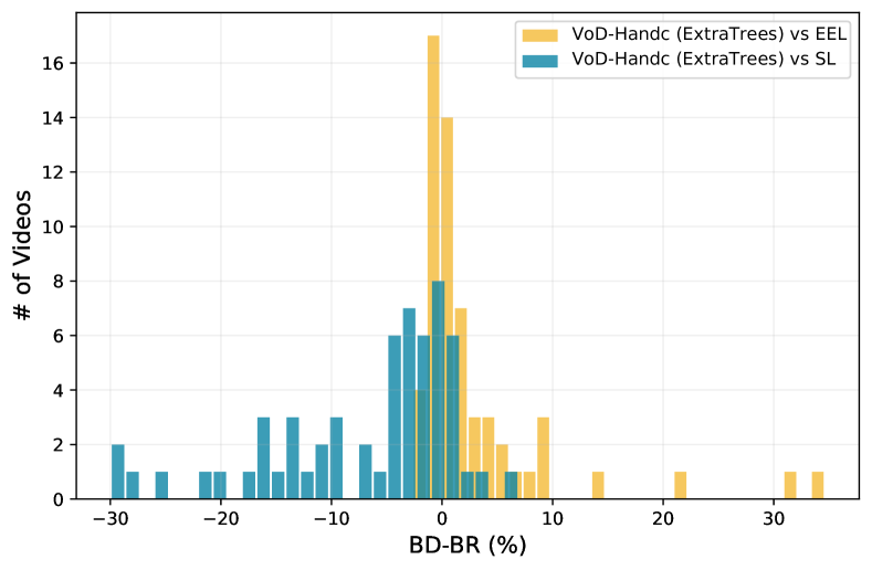
Figure 8: Histogram of BD-BR for VoD-HandC ExtraTrees model compared to EEl and SL approaches for AVC software encoding in terms of YPSNR.

V-B Coding performance

Tables IV, V, and VI give the median performance of the considered models over three stratified iterations on the AVSD dataset, using the AVC, HEVC, and VVC encoders, respectively for both YPSNR and VMAF objective quality metrics.

Table IV shows the performance of these models using AVC software and hardware encoders. The VoD-HandC features-based models consistently achieve high scores across multiple metrics in both encoding scenarios. For instance, the ExtraTrees Regressor model achieves an average accuracy of 88%/86% in predicting cross-over bitrates, resulting in a gain of 5.99%/5.58% over the static approach at the cost of a slight BD-BR loss of 1.77%/2.54% compared to the EEL method using software encoding, in terms of YPSNR/VMAF. The Live-HandC features-based models (VCA features), although not as strong as the VoD-HandC features, still outperform the static ladder (SL) approach, resulting in an average BD-BR gain of 4.95%/5.54% with software encoding and 4.33%/4.04% with hardware encoding, in terms of YPSNR/VMAF. On the other hand, DNN-based models show relatively competitive performance compared to the VoD-HandC features-based models, particularly ResNet-50, which achieved the best results among CNN baselines in both software and hardware encoding scenarios. Fig. 8 illustrates the histogram of BD-BR per tested sequence compared to EEL and SL methods. The figure shows that the bitrate gain is content dependent, ranging from -30% gain to a slight loss for a few sequences (outliers) compared to the SL method.

Table V presents the performance comparison using the HEVC encoders. The VoD-HandC feature-based (VoD-HandC) models exhibit strong performance in HEVC software encoding, notably with the ExtraTrees Regressor model achieving the highest scores in terms of YPSNR and VMAF. It outperforms the static approach with an overall gain of 5.99%/5.58% while incurring only a slight loss of 1.77%/2.54% compared to the EEL method in terms of BD-BR. Additionally, the Live-HandC feature-based (Live-HandC) models perform consistently better than the static approach SL, particularly the ExtraTrees Regressor, with an average BD-BR gain of 4.80%/5.17% using software encoding and 4.20%/3.53% using hardware encoding. In comparison, the DNN-based models, particularly ResNet-50, show competitive performance, achieving the best results among the CNN baselines in both software and hardware encoding scenarios.

Table VI compares the performance of the models considered using the VVC software encoder. Among the models considered, the ExtraTrees model, fitted with VoD-HandC features, stands out, as it achieves the highest performance in terms of YPSNR and VMAF. It outperforms the static approach with an overall gain of 5.18%/4.90% in YPSNR/VMAF while only incurring a loss of 2.86%/3.70% compared to the EEL method in terms of BD-BR. Furthermore, the Live-HandC feature-based models consistently perform better than the static approach SL, with an average BD-BR gain of 3.89%/3.41% for the best model. In terms of DNN-based models, as expected, ResNet-50 outperforms all CNN baselines with accuracy in predicting cross-over bitrates of 91%/78% in term of YPSNR.

In summary, VoD-HandC feature-based models consistently performed well across different encoding scenarios. The Live-HandC feature-based models also showed superiority over the static approach. Further, DNN-based models, particularly ResNet-50, demonstrated competitive performance compared to VoD-HandC feature-based models, which can be further optimized with a more extensive training dataset.

TABLE VII: Average inference runtime (Seconds) comparison evaluated on 10 UHD videos.

Model Features extraction Prediction CPU GPU CPU GPU VoD-HandC ExtraTrees 144.754 ✗ 0.0011 ✗ Randomforest 144.754 ✗ 0.0006 ✗ XGboost 144.754 ✗ 0.0005 ✗ LightGBM 144.754 ✗ 0.0003 ✗ Live-HandC ExtraTrees 1.086 ✗ 0.0013 ✗ Randomforest 1.086 ✗ 0.0008 ✗ XGboost 1.086 ✗ 0.0006 ✗ LightGBM 1.086 ✗ 0.0005 ✗ Deep features DensNet169 304.877 69.041 0.1720 0.0888 VGG16 473.982 67.363 0.1403 0.0625 ResNet50 273.211 63.636 0.2157 0.1013 ConvexNetBase 11729.184 146.996 0.1541 0.0744

V-C Runtime Comparison

Computational complexity is crucial to build a bitrate ladder in both VOD and live adaptive streaming applications. In this regard, we performed runtime comparisons of the compared models in this benchmark on the same desktop computer equipped with an Intel® Xeon(R) W-2133 CPU @3.60GHz $\times$12, 64G RAM, and GeForce RTX 2080 Ti graphics card under Ubuntu 20.04 long term support (LTS) operating system. Table VII gives the inference time in seconds averaged on ten random UHD video sequences from the AVSD dataset using both CPU and GPU. The table reveals that Live-HandC feature-based models achieve impressively low feature extraction times, taking less than 1.1 seconds. Moreover, the prediction time of these methods demonstrates even shorter runtime values ranging from 2 to 13 milliseconds on CPU. Thus, Live-HandC features (VCA features) are well-suited for real-time live streaming scenarios, where low latency is crucial. On the other hand, VoD-HandC feature-based models exhibit a longer feature extraction time, approximately 145 seconds, making them more suitable for VOD streaming scenarios. It should be noted that the feature extraction software may be optimized, and software optimization may result in reduced time complexity. Furthermore, deep learning models also require a long feature extraction time. For instance, ResNet50 needs approximately 273.211 seconds for feature extraction on CPU and 63.636 seconds on GPU. Nevertheless, DNN models can be further optimized to reduce inference time using pruning and knowledge-distillation techniques [67].

VI Conclusion

In this paper, we have undertaken a comprehensive review of existing methods for constructing bitrate ladders in the context of adaptive video streaming. These methods have been categorized into two main approaches: conventional and learning-based methods. Additionally, we have curated an extensive collection of video shots and have developed the largest publicly available dataset of corresponding convex hulls, referred to as AVSD. These convex hulls were generated by encoding the shots using both hardware and software video encoders, encompassing three standards: AVC/H.264, HEVC/H.265, and VVC/H.266, across four resolutions and various QP values. Furthermore, we have presented an empirical benchmark study focusing on learning-based methods for bitrate ladder prediction. The experimental results clearly demonstrate that the ExtraTrees Regressor, fitted with VoD-HandC handcrafted features, outperforms other learning-based methods when predicting cross-over bitrates. However, it is worth noting that these features can be computationally expensive and time-consuming, particularly when dealing with UHD videos, making them more suitable for VOD streaming scenarios. Moreover, our complexity analysis reveals that models based on Live-HandC features are the most suitable for live streaming applications. These features strike a balance between inference runtime and prediction performance, making them an efficient choice for such scenarios. Additionally, the promising performances of baseline CNN models suggest the significant potential of DNN approaches in addressing adaptive streaming challenges. We believe that this comprehensive benchmarking study will greatly contribute to and facilitate future research endeavors in the domain of bitrate ladder prediction for adaptive video streaming.

References

- [1] Sandvine, “Global Internet Phenomena Report 2022,” https://www.sandvine.com/phenomena, accessed on 2023-01-30.
- [2] A. Bentaleb, B. Taani, A. C. Begen, C. Timmerer, and R. Zimmermann, “A Survey on Bitrate Adaptation Schemes for Streaming Media Over HTTP,” IEEE Commun. Surveys Tuts., vol. 21, no. 1, pp. 562–585, 2019.
- [3] (2015) Per-Title Encode Optimization. [Online]. Available: https://netflixtechblog.com/per-title-encode-optimization-7e99442b62a2
- [4] N. T. Blog, “VMAF: The Journey Continues,” Oct. 2018. [Online]. Available: https://netflixtechblog.com/vmaf-the-journey-continues-44b51ee9ed12
- [5] I. Katsavounidis. (2018) Dynamic Optimizer — A Perceptual Video Encoding Optimization Framework. [Online]. Available: https://netflixtechblog.com
- [6] K. Goswami, et al., “Adaptive Multi-Resolution Encoding for ABR Streaming,” in 2018 25th IEEE International Conference on Image Processing (ICIP). IEEE, 2018, pp. 1008–1012.
- [7] M. Bhat, J.-M. Thiesse, and P. Le Callet, “A Case Study of Machine Learning Classifiers for Real-Time Adaptive Resolution Prediction in Video Coding,” in IEEE International Conference on Multimedia and Expo (ICME), 2020.
- [8] M. Takeuchi et al., “Perceptual Quality Driven Adaptive Video Coding Using JND Estimation,” in Picture Coding Symposium (PCS), 2018.
- [9] A. V. Katsenou, J. Sole, and D. R. Bull, “Content-gnostic Bitrate Ladder Prediction for Adaptive Video Streaming,” in Picture Coding Symposium (PCS), 2019.
- [10] A. V. Katsenou, F. Zhang, K. Swanson, M. Afonso, J. Sole, and D. R. Bull, “VMAF-Based Bitrate Ladder Estimation for Adaptive Streaming,” in Picture Coding Symposium (PCS), 2021.
- [11] D. Silhavy et al., “Machine Learning for Per-Title Encoding,” SMPTE Motion Imaging Journal, vol. 131, no. 3, pp. 42–50, 2022.
- [12] F. Nasiri, W. Hamidouche, L. Morin, N. Dholland, and J.-Y. Aubié, “Ensemble Learning for Efficient VVC Bitrate Ladder Prediction,” in European Workshop on Visual Information Processing (EUVIP), 2022.
- [13] V. V. Menon, H. Amirpour, M. Ghanbari, and C. Timmerer, “Perceptually-Aware Per-Title Encoding for Adaptive Video Streaming,” in IEEE International Conference on Multimedia and Expo (ICME), 2022.
- [14] T. Huang, R.-X. Zhang, and L. Sun, “Deep Reinforced Bitrate Ladders for Adaptive Video Streaming,” in in ACM Workshop on Network and Operating Systems Support for Digital Audio and Video, 2021.
- [15] (2020) Per-title encoding. [Online]. Available: https://bitmovin.com/per-title-encoding
- [16] V. V. Menon, P. T. Rajendran, C. Feldmann, K. Schoeffmann, M. Ghanbari, and C. Timmerer, “JND-aware Two-pass Per-title Encoding Scheme for Adaptive Live Streaming,” IEEE Trans. Circuits Sys. Video Technol., 2023.
- [17] T. Wiegand, G. J. Sullivan, G. Bjontegaard, and A. Luthra, “Overview of the H. 264/AVC Video Coding Standard,” IEEE Trans. Circuits Sys. Video Technol., vol. 13, no. 7, pp. 560–576, 2003.
- [18] G. J. Sullivan, J.-R. Ohm, W.-J. Han, and T. Wiegand, “Overview of the High Efficiency Video Coding (HEVC) Standard,” IEEE Trans. Circuits Sys. Video Technol., vol. 22, no. 12, pp. 1649–1668, 2012.
- [19] B. Bross, Y.-K. Wang, Y. Ye, S. Liu, J. Chen, G. J. Sullivan, and J.-R. Ohm, “Overview of the Versatile Video Coding (VVC) Standard and its Applications,” IEEE Trans. Circuits Sys. Video Technol., vol. 31, no. 10, pp. 3736–3764, 2021.
- [20] (2021) Best Practices for Creating and Deploying HTTP Live Streaming Media for the IPhone and IPad. [Online]. Available: https://developer.apple.com/documentation/http_live_streaming/http_live_streaming_hls_authoring_specification_for_apple_devices
- [21] YouTube: Choose Live Encoder Settings, Bitrates, and Resolutions. [Online]. Available: https://support.google.com/youtube/answer/2853702
- [22] Twitch. [Online]. Available: https://stream.twitch.tv/
- [23] J. De Cock, Z. Li, M. Manohara, and A. Aaron, “Complexity-Based Consistent-Quality Encoding in the Cloud,” in IEEE International Conference on Image Processing (ICIP), 2016, pp. 1484–1488.
- [24] C. Chen, Y.-C. Lin, S. Benting, and A. Kokaram, “Optimized Transcoding for Large Scale Adaptive Streaming Using Playback Statistics,” in IEEE International Conference on Image Processing (ICIP), 2018.
- [25] F. Tashtarian, A. Bentaleb, H. Amirpour, B. Taraghi, C. Timmerer, H. Hellwagner, and R. Zimmermann, “LALISA: Adaptive Bitrate Ladder Optimization in HTTP-based Adaptive Live Streaming,” in IEEE/IFIP Network Operations and Management Symposium (NOMS), 2023.
- [26] H. Amirpour, C. Timmerer, and M. Ghanbari, “PSTR: Per-Title Encoding Using Spatio-Temporal Resolutions,” in IEEE International Conference on Multimedia and Expo (ICME), 2021.
- [27] Y. A. Reznik, K. O. Lillevold, A. Jagannath, J. Greer, and J. Corley, “Optimal Design of Encoding Profiles for ABR Streaming,” in Proceedings of the 23rd Packet Video Workshop, 2018, pp. 43–47.
- [28] Y. A. Reznik, X. Li, K. O. Lillevold, A. Jagannath, and J. Greer, “Optimal Multi-Codec Adaptive Bitrate Streaming,” in IEEE International Conference on Multimedia & Expo Workshops (ICMEW), 2019.
- [29] H. Xing, Z. Zhou, J. Wang, H. Shen, D. He, and F. Li, “Predicting Rate Control Target Through A Learning Based Content Adaptive Model,” in IEEE Picture Coding Symposium (PCS), 2019.
- [30] S. Paul, A. Norkin, and A. C. Bovik, “Efficient Per-Shot Convex Hull Prediction By Recurrent Learning,” arXiv preprint arXiv:2206.04877, 2022.
- [31] H. Amirpour, M. Ghanbari, and C. Timmerer, “DeepStream: Video Streaming Enhancements using Compressed Deep Neural Networks,” IEEE Trans. Circuits Sys. Video Technol., 2022.
- [32] Z. Wang, A. C. Bovik, H. R. Sheikh, and E. P. Simoncelli, “Image quality assessment: from error visibility to structural similarity,” IEEE Trans. Image Process., vol. 13, no. 4, pp. 600–612, 2004.
- [33] L. Wang, Y. Xiong, Z. Wang, Y. Qiao, D. Lin, X. Tang, and L. Van Gool, “Temporal Segment Networks: Towards Good Practices for Deep Action Recognition,” in European conference on computer vision. Springer, 2016, pp. 20–36.
- [34] N. Ballas, L. Yao, C. Pal, and A. Courville, “Delving Deeper Into Convolutional Networks for Learning Video Representations,” arXiv preprint arXiv:1511.06432, 2015.
- [35] I. Katsavounidis, “Chimera Video Sequence Details and Scenes,” https://www.cdvl.org/documents/NETFLIX_Chimera_4096x2160_Download_Instructions.pdf, 2015.
- [36] A. Elemental, https://www.youtube.com/playlist?list=PLwIpNYl7S0G_C5I76Tf46n6ImKssMn2kT/, [Online; accessed 2018-07-02].
- [37] M. Cheon and J.-S. Lee, “Subjective and Objective Quality Assessment of Compressed 4K UHD Videos for Immersive Experience,” IEEE Trans. Circuits Sys. Video Technol., vol. 28, no. 7, pp. 1467–1480, 2017.
- [38] Harmonic Inc 4K Demo Footage, https://www.harmonicinc.com/4k-demo-footage-download/, [Online; accessed 2017-05-01].
- [39] T. U. Ultra Video Group, http://ultravideo.cs.tut.fi/, [Online; accessed 2017-01-23].
- [40] L. Song, X. Tang, W. Zhang, X. Yang, and P. Xia, “The SJTU 4K Video Sequence Dataset,” in IEEE International Workshop on Quality of Multimedia Experience (QoMEX), 2013, pp. 34–35.
- [41] Z. Li, Z. Duanmu, W. Liu, and Z. Wang, “AVC, HEVC, VP9, AVS2 OR AV1?—A Comparative Study of State-of-the-Art Video Encoders on 4K Videos,” in International Conference on Image Analysis and Recognition. Springer, 2019, pp. 162–173.
- [42] Y. Wang, S. Inguva, and B. Adsumilli, “YouTube UGC Dataset for Video Compression Research,” in IEEE International Workshop on Multimedia Signal Processing (MMSP).
- [43] Intelligent Scene Cut Detection and Video Splitting tool. [Online]. Available: https://pyscenedetect.readthedocs.io/en/latest/
- [44] S. Winkler, “Analysis of Public Image and Video Databases for Quality Assessment,” IEEE Journal of Selected Topics in Signal Processing, vol. 6, no. 6, pp. 616–625, 2012.
- [45] International Telecommunication Union, “ITU-T Recommendation P.910: Subjective Video Quality Assessment Methods for Multimedia Applications,” ITU-T, Recommendation, 2008. [Online]. Available: https://www.itu.int/rec/T-REC-P.910
- [46] M. D. Fairchild, Color Appearance Models. John Wiley & Sons, 2013.
- [47] V. V. Menon, C. Feldmann, H. Amirpour, M. Ghanbari, and C. Timmerer, “VCA: Video Complexity Analyzer,” in Proceedings of the 13th ACM Multimedia Systems Conference, 2022, pp. 259–264.
- [48] C. E. Duchon, “Lanczos Filtering in One and Two Dimensions,” Journal of Applied Meteorology and Climatology, vol. 18, no. 8, pp. 1016–1022, 1979.
- [49] Dacast, https://www.dacast.com/blog/adaptive-bitrate-streaming/, [Online; accessed 2023-03-02].
- [50] FFmpeg. [Online]. Available: https://www.ffmpeg.org/
- [51] A. Wieckowski et al., “VVenC: An Open and Optimized VVC Encoder Implementation,” in IEEE International Conference on Multimedia & Expo Workshops (ICMEW), 2021.
- [52] M. Afonso, F. Zhang, and D. R. Bull, “Spatial Resolution Adaptation Framework for Video Compression,” in Applications of Digital Image Processing XLI, vol. 10752. SPIE, 2018, pp. 209–218.
- [53] A. Telili, W. Hamidouche, S. A. Fezza, and L. Morin, “Benchmarking Learning-Based Bitrate Ladder Prediction Methods for Adaptive Video Streaming,” in Picture Coding Symposium (PCS), 2022, pp. 325–329.
- [54] R. M. Haralick, K. Shanmugam, and I. H. Dinstein, “Textural Features for Image Classification,” IEEE Trans. Syst., Man, Cybem., no. 6, pp. 610–621, 1973.
- [55] A. V. Katsenou, M. Afonso, D. Agrafiotis, and D. R. Bull, “Predicting Video Rate-Distortion Curves Using Textural Features,” in Picture Coding Symposium (PCS), 2016.
- [56] C. Liu, W. T. Freeman, R. Szeliski, and S. B. Kang, “Noise Estimation from A Single Image,” in IEEE Computer Society Conference on Computer Vision and Pattern Recognition (CVPR’06), vol. 1, 2006, pp. 901–908.
- [57] J. P. Lewis, “Fast Template Matching,” in Vision interface, vol. 95, no. 120123. Quebec City, QC, Canada, 1995, pp. 15–19.
- [58] P. Geurts, D. Ernst, and L. Wehenkel, “Extremely Randomized Trees,” Machine learning, vol. 63, pp. 3–42, 2006.
- [59] J. Deng, W. Dong, R. Socher, L.-J. Li, K. Li, and L. Fei-Fei, “Imagenet: A Large-Scale Hierarchical Image Database,” in IEEE conference on computer vision and pattern recognition, 2009, pp. 248–255.
- [60] X. Zhang, J. Zou, K. He, and J. Sun, “Accelerating Very Deep Convolutional Networks for Classification and Detection,” IEEE Trans. Pattern. Anal. Mach. Intell., vol. 38, no. 10, pp. 1943–1955, 2015.
- [61] G. Huang, Z. Liu, L. Van Der Maaten, and K. Q. Weinberger, “Densely Connected Convolutional Networks,” in IEEE conference on computer vision and pattern recognition, 2017, pp. 4700–4708.
- [62] K. He, X. Zhang, S. Ren, and J. Sun, “Deep Residual Learning for Image Recognition,” in IEEE conference on computer vision and pattern recognition, 2016, pp. 770–778.
- [63] Z. Liu, H. Mao, C.-Y. Wu, C. Feichtenhofer, T. Darrell, and S. Xie, “A Convnet for the 2020s,” in IEEE/CVF Conference on Computer Vision and Pattern Recognition, 2022, pp. 11 976–11 986.
- [64] T. K. Ho, “Random Decision Forests,” in IEEE international conference on document analysis and recognition, vol. 1, 1995, pp. 278–282.
- [65] T. Chen et al., “XGBoost: Extreme Gradient Boosting,” R package version 0.4-2, vol. 1, no. 4, pp. 1–4, 2015.
- [66] G. Ke, Q. Meng, T. Finley, T. Wang, W. Chen, W. Ma, Q. Ye, and T.-Y. Liu, “Lightgbm: A Highly Efficient Gradient Boosting Decision Tree,” Advances in neural information processing systems, vol. 30, 2017.
- [67] C. Morris, D. Danier, F. Zhang, N. Anantrasirichai, and D. R. Bull, “ST-MFNet Mini: Knowledge Distillation-Driven Frame Interpolation,” arXiv preprint arXiv:2302.08455, 2023.