Unlocking the Transferability of Tokens in Deep Models for Tabular Data

Abstract

Fine-tuning a pre-trained deep neural network has become a successful paradigm in various machine learning tasks. However, such a paradigm becomes particularly challenging with tabular data when there are discrepancies between the feature sets of pre-trained models and the target tasks. In this paper, we propose TabToken, a method aims at enhancing the quality of feature tokens (i.e., embeddings of tabular features). TabToken allows for the utilization of pre-trained models when the upstream and downstream tasks share overlapping features, facilitating model fine-tuning even with limited training examples. Specifically, we introduce a contrastive objective that regularizes the tokens, capturing the semantics within and across features. During the pre-training stage, the tokens are learned jointly with top-layer deep models such as transformer. In the downstream task, tokens of the shared features are kept fixed while TabToken efficiently fine-tunes the remaining parts of the model. TabToken not only enables knowledge transfer from a pre-trained model to tasks with heterogeneous features, but also enhances the discriminative ability of deep tabular models in standard classification and regression tasks.

1 Introduction

Deep learning has achieved remarkable success in various domains, including computer vision [52] and natural language processing [40]. While these fields have benefited greatly from deep learning, the application of deep models to tabular data is difficult [18, 20]. Highly structured, tabular data is organized with rows representing individual examples and columns corresponding to specific features. Within domains such as finance [1], healthcare [22], and e-commerce [37], tabular data emerges as a common format where classical machine learning methods like XGBoost [12] have showcased strong performance. In recent years, deep models have been extended to tabular data, leveraging the ability of deep neural networks to capture complex feature interactions and achieve competitive results compared to boosting methods in certain tasks [13, 21, 41, 5, 18, 31, 10, 11, 25].

The “pre-training then fine-tuning” paradigm is widely adopted in deep learning. By reusing the pre-trained feature extractor, the entire model is subsequently fine-tuned on target datasets [16, 55, 48, 49, 47]. However, when it comes to tabular data, the transferability of pre-trained deep models faces unique challenges. The tabular features often possess semantic meanings and the model attempts to comprehend the relationships between features and targets. Each tabular feature has strong correspondence with model parameters, making it hard to directly transfer pre-trained deep learning models when encountering unseen features [53, 15, 23, 39, 62]. For instance, different branches of financial institutions may share certain features when predicting credit card fraud, but each branch may also possess unique features associated with their transaction histories. Besides, the scarcity of available samples for fine-tuning on new datasets further complicates the knowledge transfer process.

In this paper, we focus on a crucial component of tabular deep models — the feature tokenizer, which is an embedding layer that transforms numerical or categorical features into high-dimensional vectors (tokens). The original features correspond specifically with these tokens, which are leveraged by the top-layer models like transformers [51] and Multi-Layer Perceptrons to extract relationships between features [18, 19]. Through the feature tokenizer, all features are transformed in the same manner, the tokens seem to be a tool to bridge two heterogeneous feature sets by reusing tokens of shared features in a pre-trained model. By transferring the feature tokens, the model achieves a reduction in the size of learnable parameters. The model may leverage knowledge acquired from pre-training data and enhance its generalization ability on the target dataset.

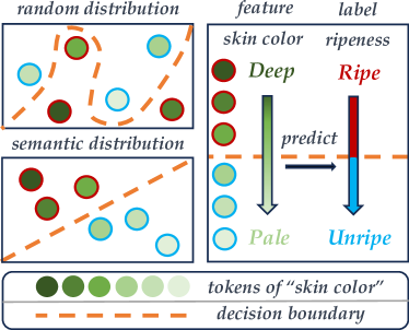
Figure 1: The toy example involves predicting ripeness based on the color of the watermelon, where ripe ones have a deep color and unripe ones are pale. Semantic distributions are more discriminative and possess the potential for transferability.

However, our observation reveals that the learned tokens exhibit random behavior and lack discriminative properties. Since learning the feature relationships is crucial as it enables the model to gain a deeper understanding of the underlying patterns within the data, the top-layer models encounter more difficulties in effectively learning from the semantically deficient tokens. As illustrated in Figure 1, if the feature tokens corresponding to the six possible values of “skin color” are randomly distributed, the decision boundary becomes complex. The correlation between skin color and ripeness needs to be learned by a more complex top-layer model. However, with a discriminative semantic distribution, a simple classifier can achieve accurate predictions. At this point, the tokens will contain potentially transferable knowledge, which may unlock the transferability of feature tokens.

To address this issue, we propose TabToken to introduce semantics to feature tokens, improving the transferability of feature tokenizers. Specifically, TabToken aims to leverage the semantic information provided by the instance labels to understand feature relationships. Firstly, we represent an instance by averaging the tokens associated with all features. Based on the instance tokens, we introduce a contrastive token regularization objective that minimizes the distance between instances and their respective class centers. By incorporating this regularization into the pre-training stages, TabToken enables the previously randomly distributed feature tokens to reflect actual semantic information, bolstering the model’s transferability. Furthermore, the fine-tuning stage benefits from the enhanced pre-trained feature tokens, learning new modules under the constraint of regularization.

Our experiments demonstrate the efficacy of TabToken in achieving model transfer across datasets with heterogeneous feature sets. TabToken also improves the performance of deep models in standard tabular tasks involving classification and regression. The contributions of our paper are:

• We emphasize the significance of token quality in facilitating the transferability of tabular deep models when there is a change in the feature set between pre-training and downstream datasets. To the best of our knowledge, we are the first to focus on feature tokens in tabular transfer learning.

• We introduce TabToken to enhance the transferability of deep tabular models by incorporating feature semantics into the tokens and enabling their utilization in downstream tasks.

• Through experiments on real-world datasets, we demonstrate the ability of TabToken to reveal explainable feature semantics. Furthermore, our method showcases strong performance in heterogeneous transfer tasks as well as standard tabular tasks.

2 Related Work

Standard Tabular Data Learning. Tabular data is a prevalent data format in numerous real-world applications, spanning click-through rate prediction [43], fraud detection [6], and time-series forecasting [2]. Traditional machine learning methods for tabular data mainly focus on feature engineering and hand-crafted feature selection. Popular algorithms encompass decision trees, random forests, and gradient boosting machines. Among them, XGBoost [12], LightGBM [32], and CatBoost [42] are widely employed tree-based models that exhibit comparable performance for tabular data. Deep learning models have shown promise in automatically learning feature representations from raw data and have achieved competitive performance across diverse tabular data applications, such as click-through rate prediction [59] and time-series forecasting [35].

Deep Tabular Data Learning. Recently, a large number of deep learning models for tabular data have been developed [13, 21, 5, 18, 41, 10, 31, 11, 25]. These models either imitate the tree structure or incorporate popular deep learning components. They have demonstrated superior performance compared to traditional machine learning methods, especially in sparse and high-dimensional feature spaces. However, deep learning models for tabular data struggle to learn high-order feature interactions [20], which are crucial in many tabular data applications, and require substantial amounts of training data. Boosting methods [12, 32, 42] can effectively capture these interactions and are more robust to data limitations. While deep models may not surpass tree-based models entirely on tabular data, they offer greater flexibility and can be customized for complex and specific tasks, especially when faced with changing factors such as features and labels.

Transferring Tabular Models across Feature Spaces. Transferring knowledge from pre-trained models across feature spaces can be challenging but also beneficial, as it reduces the need for extensive data labeling and enables efficient knowledge reuse [54, 28, 60, 57, 26, 27]. In real-world applications such as healthcare, there are numerous medical diagnostic tables. These tables usually have some features in common such as blood type and blood pressure. For rare diseases with limited data, knowledge transfer from other diagnostic tables with overlapping features becomes beneficial. When feature space changes, language-based methods assume there are semantic relationships between the descriptions of features [53, 15, 23], and rely on large-scale language models.

However, sufficient textual descriptions are not always the case in tabular data. Without the requirement for language, Pseudo-Feature method [34] utilize pseudo-feature models individually for each new feature, which is computationally expensive in our broader feature space adaptation and require access to pre-training data. TabRet [39] utilizes masked autoencoding to make transformer work in downstream tasks. XTab [62] enhances the transferability of the transformer (one type of the top-layer models), while we discover the untapped potential in improving the feature tokens and develop a tokenizer with stronger transferability. To transfer pre-trained large language models to tabular tasks, ORCA [45] trains an embedder to align the source and target distributions. Our approach, on the other hand, centers on how to directly transfer the embedder (tokenizer). In contrast to prior work, our emphasis lies in enhancing the quality of feature tokens and unlocking their transferability.

3 Preliminary and Background

In this section, we introduce the task learning with tabular data, as well as the vanilla deep tabular models based on feature tokens. We also describe the scenario of transferring a pre-trained model to downstream tasks with heterogeneous feature sets.

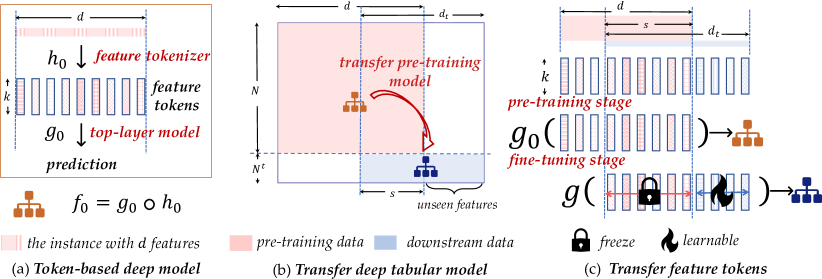
Figure 2: Illustrations of the token-based model, transfer task, and the procedure of TabToken. (a) The token-based models $f_{0}$ for tabular data can be decomposed into a feature tokenizer $h_{0}$ and a top-layer model $g_{0}$. (b) In the transfer task, the downstream dataset consists of $s$ overlapping features with the pre-training dataset while also introducing $d_{t}-s$ unseen features. When the feature space changes, we expect to transfer the pre-trained model for downstream tasks. (c) In the pre-training stage, by employing token combination and regularization, TabToken incorporates the semantics of labels into tokens. In the fine-tuning stage, TabToken freezes the overlapping feature tokens of the pre-trained tokenizer, efficiently fine-tuning other modules.

3.1 Learning with Tabular Data

Given a labeled tabular dataset $\mathcal{D}=\{({\bm{x}}_{i,:},y_{i})\}_{i=1}^{N}$ with $N$ examples (rows in the table). An instance ${\bm{x}}_{i,:}$ is associated with a label $y_{i}$. We consider three types of tasks: binary classification $y_{i}\in\{0,1\}$, multiclass classification $y_{i}\in[C]=\{1,\ldots,C\}$, and regression $y_{i}\in\mathbb{R}$. There are $d$ features (columns) for an instance ${\bm{x}}_{i,:}$, we denote the $j$-th feature in tabular dataset as ${\bm{x}}_{:,j}$. The tabular features include numerical (continuous) type ${\bm{x}}_{:,j}^{\textit{\rm num}}$ and categorical (discrete) type ${\bm{x}}_{:,j}^{\textit{\rm cat}}$. Denote the $j$-th feature value of ${\bm{x}}_{i,:}$ as $x_{i,j}$. We assume $x_{i,j}^{\textit{\rm num}}\in\mathbb{R}$ when it is numerical (e.g., the salary of a person). While for a categorical feature (e.g., the occupation of a person) with $K_{j}$ discrete choices, we present ${\bm{x}}_{i,j}^{\textit{\rm cat}}\in\{0,1\}^{K_{j}}$ in a one-hot form, where a single element is assigned a value of 1 to indicate the categorical value. We learn a model $f_{0}$ on $\mathcal{D}$ that maps ${\bm{x}}_{i,:}$ to its label $y_{i}$, and a generalizable model could extend its ability to unseen instances sampled from the same distribution as $\mathcal{D}$.

3.2 Token-based Methods for Tabular Data

There are several classical methods when learning on tabular data, such as logistic regression (LR) and XGBoost. Similar to the basic feature extractor when applying deep models over images and texts, one direct way to apply deep learning models on the tabular data is to implement model $f_{0}$ with Multi-Layer Perceptron (MLP) or Residual Network (ResNet). While for token-based deep learning models, the model $f_{0}$ is implemented by the combination of feature tokenizer $h_{0}$ and top-layer deep models $g_{0}$. The prediction for instance ${\bm{x}}_{i,:}$ is denoted as $f_{0}({\bm{x}}_{i,:})=g_{0}\circ h_{0}({\bm{x}}_{i,:})=g_{0}(h_{0}({\bm{x}}_{i,:}))$. We minimize the following objective to obtain the feature tokenizer $h_{0}$ and top-layer model $g_{0}$:

$$\min_{f_{0}=g_{0}\circ h_{0}}\sum_{i=1}^{N}\left[\ell\left(g_{0}\circ h_{0}({\bm{x}}_{i,:}),y_{i}\right)\right],$$ (1)

where the loss function $\ell(\cdot,\cdot)$ measures the discrepancy between the prediction and the label. Feature tokenizer $h_{0}$ performs a similar role to the feature extractor in traditional image models [17, 18]. It maps the features to high-dimensional tokens in a hidden space, facilitating the learning process of top-layer $g_{0}$. The top-layer model $g_{0}$ infers feature relationships based on the feature tokenizer $h_{0}$ and then performs subsequent classification or regression tasks.

Feature Tokenizer. We follow FT-trans [18] to implement the feature tokenizer. The tokenizer $h_{0}$ transforms the input ${\bm{x}}_{i,:}$ into a $d\times k$ matrix $\{\hat{{\bm{x}}}_{i,j}\}_{j=1}^{d}$. In detail, for a numerical feature value $x_{i,j}^{\textit{{\rm num}}}\in\mathbb{R}$, it is transformed as $\hat{{\bm{x}}}_{i,j}=x_{i,j}^{\textit{\rm num}}\cdot\bm{E}^{\textit{\rm num}}_{j}$, where $\bm{E}^{\textit{\rm num}}_{j}$ is a learnable $k$-dimensional vector (token) for the $j$-th feature. For a categorical feature ${\bm{x}}_{i,j}^{\textit{\rm cat}}\in\{0,1\}^{K_{j}}$, where there are $K_{j}$ discrete choices, the tokenizer is implemented as a lookup table. Given $\bm{E}^{\textit{\rm cat}}_{j}\in\mathbb{R}^{K_{j}\times k}$ as the set of $K_{j}$ tokens, the tokenizer transform ${\bm{x}}_{i,j}^{\textit{\rm cat}}$ as $\hat{{\bm{x}}}_{i,j}={{\bm{x}}_{i,j}^{\textit{\rm cat}}}^{\top}\bm{E}^{\textit{\rm cat}}_{j}$. Overall, the feature tokenizer maps different types of features to a unified form — ${\bm{x}}_{i,:}$ is transformed into a $d\times k$ matrix $\{\hat{{\bm{x}}}_{i,j}\}_{j=1}^{d}$ with a set of $k$-dimensional tokens. The model learns feature tokens $\bm{E}^{\textit{\rm num}}$ or $\bm{E}^{\textit{\rm cat}}$ during the training process. The feature tokenizer $h_{0}$ is a weighted or selective representation of feature tokens.

Deep Top-layer Models. After the tokenizer, the transformed tokens $h_{0}({\bm{x}}_{i,:})=\{\hat{{\bm{x}}}_{i,j}\}_{j=1}^{d}$ for instance ${\bm{x}}_{i,:}$ are feed into top-layer models. There can be various top-layer models, such as MLP, ResNet, and transformer. When the top-layer model is MLP or ResNet, it cannot directly process the set of tokens $h_{0}({\bm{x}}_{i,:})$. The common approach is to concatenate $d$ tokens into a long $dk$-dimensional vector ${\bm{T}}^{\textit{\rm con}}_{i}\in\mathbb{R}^{dk}$. Then, ${\bm{T}}^{\textit{\rm con}}_{i}$ feeds into the top-layer model $g_{0}$:

$$f_{0}({\bm{x}}_{i,:})=g_{0}({\bm{T}}^{\textit{\rm con}}_{i}),\;{\bm{T}}^{\textit{\rm con}}_{i}={\rm concat}(h_{0}({\bm{x}}_{i,:}))\;.$$ (2)

For the transformer, the token set of ${\bm{x}}_{i,:}$ directly feeds into the transformer layer without the need for concatenating. The input $h_{0}\left({\bm{x}}_{i,:}\right)$ and output $\bm{F}_{i}$ of transformer are both a set of $k$-dimension tokens

$$\bm{F}_{i}={\rm TransformerLayer}\left(\ldots\left({\rm TransformerLayer}\left(h_{0}\left({\bm{x}}_{i,:}\right)\right)\right)\right)\in\mathbb{R}^{d\times k},$$

where the module ${\rm TransformerLayer}(\cdot)$ is described in  Appendix B. Based on the transformed tokens, the results could be obtained based on a prediction head over the averaged token:

$$f_{0}({\bm{x}}_{i,:})={\rm Prediction}\left(\frac{1}{d}{\sum_{j=1}^{d}{\bm{F}}_{i,j}}\right),$$

where $\bm{F}_{i,j}$ is the $j$-th token in the output token set $\bm{F}_{i}$ of transformer. The head ${\rm Prediction}(\cdot)$ consists of an activation function ReLU and a fully connected layer.

3.3 Transfer Learning with Overlapping and Unseen Features

Given another related downstream dataset $\mathcal{D}^{t}=\{({\bm{x}}_{i,:}^{t},y_{i}^{t})\}_{i=1}^{N^{t}}$ with $N^{t}$ examples ($N^{t}\ll N$) and $d_{t}$ features, we aim to construct a new model $f$ for $D^{t}$ borrowing the knowledge of well-trained $f_{0}$. We assume there exists heterogeneity between $\mathcal{D}$ and $\mathcal{D}^{t}$, in their feature or label sets. We mainly consider the scenario that $\mathcal{D}$ and $\mathcal{D}^{t}$ have the same label space but different feature spaces. We explore different label spaces in subsection D.2. We denote the features ranging from the $j$-th to the $m$-th as $\{{\bm{x}}_{:,j:m}\}$. The last $s$ features $\{{\bm{x}}_{:,d-s+1:d}\}$ in the pre-trained dataset are shared features (overlapping features), corresponding to the first $s$ features $\{{\bm{x}}_{:,1:s}^{t}\}$ in the fine-tuning dataset. The unseen feature set in the downstream dataset is $\{{\bm{x}}_{:,s+1:d_{t}}^{t}\}$. We pre-train $h_{0}$ and $g_{0}$ together on $\mathcal{D}$, then we fine-tune $f=g\circ h$ on $\mathcal{D}^{t}$. Our goal (illustrated in Figure 2) is to train $f$ with strong generalization ability in downstream tasks.

Inspired by the idea of “pre-training then fine-tuning” in traditional deep learning, since feature tokenizer $h_{0}$ is pre-trained on sufficient examples, we expect to reuse its weights $\{\bm{E}^{\textit{\rm num}}_{j}\}_{j=1}^{d}$ or $\{\bm{E}^{\textit{\rm cat}}_{j}\}_{j=1}^{d}$ to construct a better fine-tuning feature tokenizer $h$. As each token from the tokenizer is correspond to a specific feature and there are overlapping features $\{{\bm{x}}_{:,d-s+1:d}\}$, it should be possible to reuse the token directly when the feature space changes. The knowledge acquired from the upstream task appears to be present in the pre-trained feature tokens.

However, our observation experiments (in section 5) show that the tokens generated during the vanilla pre-training process display stochastic patterns. These feature tokens lack sufficient semantic information, hindering their ability to reflect discriminative feature relationships, thereby limiting their effectiveness in aiding top-layer models and transferability in transfer learning.

4 Improve Feature Tokens for Transferable Deep Tabular Models

To address the issue that the feature tokens obtained through vanilla training are distributed in an almost random manner, we analyze the significance of semantics in unlocking feature tokens’ transferability, and propose a pre-training then fine-tuning procedure for transfer tasks.

4.1 Token Semantics Play a Role in Transferability

Since the feature tokens are in correspondence with features, tokens should reflect the nature of features, implying that tokens may carry semantics. However, based on our analysis in Appendix A, feature tokenizer does not increase the model capacity. During vanilla training, different tokens are concatenated and then predicted by different parts of the classifier. Considering an extreme scenario, the model could accurately predict an instance even when feature tokens are generated randomly, by only optimizing the classifier. Consequently, as long as the top-layer model is sufficiently strong for the current task, the trained tokens do not retain enough knowledge for transfer.

Tokens that lack semantics or even resemble randomness lack discriminative power and hold little value for transfer. Unlike in the image or text domains, where the feature extractors capture the semantic meaning with their strong capacity and enable model transferability across tasks [46, 14], unlocking the transferability of feature tokenizer in the tabular model is challenging. Without additional information, it is difficult to directly learn semantically meaningful tokens. The downstream task also fails to transfer the learned knowledge in overall model due to different feature space. To make the tokens of sharing feature transferable, it is important to introduce token semantics.

4.2 Semantic Enriched Pre-Training

The label assigned to an instance could be additional information that help feature tokens understand semantics. For example, for the feature “occupation” with values like “entrepreneur”, “manager”, and “unemployed", if the label indicates whether the individual has a credit risk, typically, the labels for “entrepreneur” and “manager” would be low risk, while “unemployed” might be associated with high risk. By grouping instances with the same label together, semantically similar tokens corresponding to “entrepreneur” and “manager” would cluster. Therefore, to achieve the goal of imbuing tokens with semantics, we utilize instance labels as additional supervision.

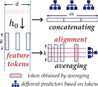
Figure 3: Averaging outperforms concatenating as it aligns distinct feature tokens, which enhances the semantics.

To facilitate direct distance computation for grouping instances, we need to represent each instance by one token instead of a token set. Token combination transforms the set of tokens $h_{0}({\bm{x}}_{i,:})=\{\hat{{\bm{x}}}_{i,j}\}_{j=1}^{d}$ into an instance token $\bm{T}_{i}$ of ${\bm{x}}_{i,:}$. As in  Equation 2, the usual combination operation is concatenating, which makes $\bm{T}_{i}^{\textit{\rm con}}$ a high-dimensional vector. However, when the order of input features is permuted, applying concatenating to the same ${\bm{x}}_{i,:}$ after the feature tokenizer will result in different $\bm{T}_{i}^{\textit{\rm con}}$. Besides, the vector values at the same position in different feature tokens will correspond to different weights in the subsequent predictor (as shown in Figure 3). This implies that, for different features ${\bm{x}}_{:,m}$ and ${\bm{x}}_{:,n}(m\neq n)$, the meanings of $\hat{{\bm{x}}}_{i,m}\in\mathbb{R}^{k}$ and $\hat{{\bm{x}}}_{i,n}\in\mathbb{R}^{k}$ are not the same in the corresponding dimension. Therefore, concatenating fails to consider the alignment between features.

Instead, we propose utilizing averaging for token combination, which averages the vector values at the same position in different feature tokens. Averaging also makes instance tokens remain unchanged regardless of the order of input features. We obtain the representation $\bm{T}_{i}^{\textit{\rm avg}}\in\mathbb{R}^{k}$ for instance ${\bm{x}}_{i}$ in the following form: $\bm{T}_{i}^{\textit{\rm avg}}=\frac{1}{d}\sum_{j=1}^{d}\hat{{\bm{x}}}_{i,j}.$ For notational clarity, we drop the superscript avg of $\bm{T}_{i}^{\textit{\rm avg}}$. We calculate the the class center $\bm{S}_{y_{i}}\in\mathbb{R}^{k}$ for ${\bm{x}}_{i,:}$ by averaging instance tokens belong to the same class: $\bm{S}_{y_{i}}=\frac{1}{N^{y_{i}}}\sum_{y_{p}=y_{i}}\bm{T}_{p}$, where $\{\bm{T}_{p}\}_{y_{p}=y_{i}}$ are the $N^{y_{i}}$ instance tokens with the same class to ${\bm{x}}_{i,:}$. $\bm{S}_{y_{i}}$ is the class center belongs to the label $y_{i}$ of ${\bm{x}}_{i,:}$. We anticipate that instance tokens belonging to the same class will exhibit proximity [56]. As instance tokens are derived from averaging the feature tokens, the tokens that share similar semantic relevance to the label should cluster together. Therefore, we pull instance tokens toward their class center via a contrastive regularization $\Omega:\mathbb{R}^{N\times k}\rightarrow\mathbb{R}$:

$$\Omega\left(\{\bm{T}_{i}\}_{i=1}^{N}\right)=\frac{1}{N}\sum_{i=1}^{N}\left\|\bm{T}_{i}-\bm{S}_{y_{i}}\right\|^{2}_{2}.$$

We name this contrastive regularization as “Contrastive Token Regularization (CTR)”. For token regularization, we calculate the regularization term on instance tokens and add the term to training loss $\ell$. The objective is to minimize the following loss:

$$\min_{f_{0}=g_{0}\circ h_{0}}\sum_{i=1}^{N}\left[\ell(g_{0}\circ h_{0}({\bm{x}}_{i,:}),y_{i})\right]+\beta\Omega\left(\{\bm{T}_{i}\}_{i=1}^{N}\right),$$ (3)

where $\beta$ is a hyperparameter that controls the regularization term. In the pre-training stage, we learn the feature tokenizer $h_{0}$ and the top-layer model $g_{0}$ simultaneously. Different from the objective in Equation 1, the feature tokens $\{\bm{E}^{\textit{\rm num}}_{j}\}_{j=1}^{d}$ or $\{\bm{E}^{\textit{\rm cat}}_{j}\}_{j=1}^{d}$ are subject to two constraints. Firstly, they need to be adjusted in a way that enhances the predictions of the top-layer model. Secondly, a regularization is employed to ensure that the tokens retain their semantic.

In practice, only the samples within each batch are used to compute the center. For regression tasks, the regularization term is computed by dividing the target values into two pseudo-classes. We use the median as a threshold. For instance, if the median of the target values in the dataset is 0.5, samples with values greater than 0.5 are labeled as class 1, while less than 0.5 are labeled as class 2. These pseudo-labels are only utilized for computing the CTR. In Appendix D, we compare the effect of CTR with other contrastive losses, verifying that our simple regularization has obvious advantages.

4.3 Token Reused Fine-tuning

Through the utilization of the CTR, we can enhance the feature tokenizer during the pre-training stage. In this subsection, we elucidate the reuse process based on high-quality tokens. We pre-train $g_{0}\circ h_{0}$ with CTR, which is essential for the transferability of feature tokens. For the ease of expression, we use $\{\bm{E}_{j}^{\textit{\rm pre}}\}_{j=1}^{d}$ to represent $\{\bm{E}^{\textit{\rm num}}_{j}\}_{j=1}^{d}$ or $\{\bm{E}^{\textit{\rm cat}}_{j}\}_{j=1}^{d}$, which are the feature tokens of the pre-training feature tokenizer $h_{0}$. In the transfer task, we expect to reuse $\{\bm{E}_{j}^{\textit{\rm pre}}\}_{j=1}^{d}$ to construct fine-tuning feature tokenizer $h$, then we fine-tuning $g\circ h$ on downstream dataset $\mathcal{D}^{t}$.

There are $d$ pre-training features $\{{\bm{x}}_{:,1:d}\}$ and $d_{t}$ downstream features $\{{\bm{x}}_{:,1:d_{t}}^{t}\}$. As illustrated in  Figure 2(b), in the downstream task, there are two feature sets: $s$ overlapping features $\{{\bm{x}}_{:,1:s}^{t}\}(\{{\bm{x}}_{:,d-s+1:d}\})$ and $d_{t}-s$ unseen features $\{{\bm{x}}_{:,s+1:d_{t}}^{t}\}$. To construct the fine-tuning tokenizer $h$, for overlapping features, $h$ fix the pre-trained feature tokens $\{\bm{E}_{j}^{\textit{\rm pre}}\}_{j=d-s+1}^{d}$ of $h_{0}$ and transfer. For unseen features, $h$ firstly initializes the remaining feature tokens based on the averaging of all pre-trained feature tokens: $\frac{1}{d}\sum_{j=1}^{d}\bm{E}_{j}^{\textit{\rm pre}}\in\mathbb{R}^{k}$. Then $h$ fine-tunes these learnable tokens.

After building $h$, we freeze the overlapping feature tokens. The learnable modules are top-layer model $g$ (transformer) and unseen feature tokens in $h$. To regularize feature tokens for unseen features, we utilize averaging and CTR to perform fine-tuning, too. Continuing with the notations from Equation 3, we optimize model $f=g\circ h$ via minimizing the following objective on downstream dataset $\mathcal{D}^{t}$:

$$\min_{f=g\circ h}\quad \sum_{i=1}^{N^{t}}\left[\ell(g\circ h({\bm{x}}_{i,:}^{t}),y_{i}^{t})\right]+\beta\cdot\frac{1}{N^{t}}\sum_{i=1}^{N^{t}}\left\|\bm{T}_{i}-\bm{S}_{y_{i}^{t}}\right\|^{2}_{2}$$

s.t. $$h({\bm{x}}_{i,:}^{t})=H({\bm{x}}_{i,:}^{t}),\;$$

$$H({\bm{x}}_{i,j}^{t})=\begin{cases}h_{0}({\bm{x}}_{i,j}^{t}),&1\leq j\leq s,\\ \hat{{\bm{x}}}_{i,j}^{t},&s+1\leq j\leq d_{t},\end{cases}$$

where $h_{0}$ remains fixed and $\beta$ is a pre-defined coefficient for adjusting the regularization term.

Summary of TabToken. When there is a change in the feature space, we aim to transfer the tokens corresponding to shared features. In the pre-training stage, we enhance the quality of tokens by introducing semantics, making them transferable. In the fine-tuning stage, we continue to constrain new feature tokens using both the frozen pre-trained feature tokens and CTR. TabToken unlocks the tokens’ transferability through a well-designed combination of pre-training and fine-tuning processes.

5 Visualization on Token Semantics

We visualize the impact of vanilla training and TabToken on feature tokens by training on a real-world dataset bank-marketing and a synthetic dataset. The synthetic dataset helps to understand CTR’s behavior in controlled conditions. The bank-marketing dataset demonstrates that our method generalizes well to real-world applications. Different from visualizations on the penultimate layer’s embeddings [29], the feature tokens are feature-specific embeddings near the input of the tabular model, which better reveals the quality of the feature tokenizer.

5.1 Semantical Relationships between Different Features

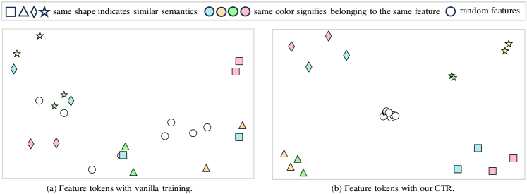
Figure 4: Feature tokens on synthetic datasets. Colors indicate which feature the tokens belong to, and the same shapes indicate semantically similar tokens. Colorless circles represent tokens of random features. (a): Categories with similar semantics across different features are not captured in the tokens. Tokens from random features may come close to other tokens that are relevant to the target, thereby influencing the prediction. (b): Tokens with similar semantics exhibit a clear clustering phenomenon, while tokens representing random features are tightly clustered together in the center.

We construct a synthetic four-class classification dataset consisting of 6 features, each feature with 4 categorical choices. In feature tokenizer, each discrete categorical choice has a corresponding token, after training we can get $6\times 4=24$ feature tokens. The details of synthetic datasets are in Appendix C.

Semantically Similar Feature Tokens. We construct highly correlated features as follows: when we generate an instance, two different features have a one-to-one correspondence with the categorical choices. As in the real-world data, “fireman” of feature “occupation” always appears together with “male” of feature “gender”. “fireman” and “male” exhibit a strong correlation. The relationship between the features and labels we set in the synthetic dataset is closely tied to the feature values. As a result, these semantically similar tokens come from different features. We expect these tokens to be close to each other.

Random Feature Tokens. We construct noise features, whose values are random. We expect that random feature tokens should have a distance from feature tokens that contribute to predictions. Otherwise random feature tokens will exert similar influences on the subsequent top-layer model’s prediction process, which is not the desired outcome.

We simply train a one-layer Linear model upon a feature tokenizer. The dimension of the token is set to 2 for better visualization, and the results of the feature tokens after training are shown in Figure 4. For semantically similar features (distinguished by shape), feature tokens generated with vanilla training exhibit a random distribution, showing no discernible patterns. While if feature tokenizer is trained with CTR, all groups of tokens are separately clustered together. TabToken enables the trained feature tokens to capture the semantic correlation between different features.

For random feature tokens (the colorless circles), when CTR is not employed, some random tokens are closely located to those semantically meaningful features. When the random tokens are trained with CTR, they occupy the same region in the latent space, staying away from other feature tokens. The reason why these tokens are clustered together is that, random features do not contribute to label predictions, during the training process, they are under the constraint of the CTR. The phenomenon of complete clustering satisfies the regularization term that reduces the distance between instance tokens of the same class. Therefore, it helps indicate noise features that do not contribute to prediction.

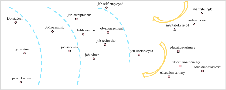
Figure 5: Feature tokens trained with CTR on bank-marketing dataset. The tokens of feature “job” depict a distribution based on job types. The hierarchical pattern is in relation to the probability associated with purchasing financial products. The distribution of tokens for the feature “education” and feature “marital” aligns perfectly with their respective semantic order.

5.2 Category Relationships within Single Feature

Within a single categorical feature, there may be semantic relationships among different discrete choices. We selected three categorical features, “job”, “education”, and “marital”, from the real-world dataset “bank-marketing”. The target of the “bank-marketing” is to predict the success rate of a customer purchasing financial products. There are inherent relationships between different categorical values of single features. We train a three-layer transformer on a 64-dimensional feature tokenizer. After training, we employed t-SNE to reduce their feature tokens to 2 dimensions for observation.

Figure 5 shows the results of feature tokens. The feature tokens obtained by CTR can indicate the arrangement of the tokens within a single feature. There are semantic arrangements within the features, such as “tertiary” $\rightarrow$ “secondary” $\rightarrow$ “primary” in feature “education”, “divorced” $\rightarrow$ “married” $\rightarrow$ “single” in feature “marital”. Besides, the tokens associated with the feature “job” exhibit a hierarchical pattern, where certain jobs like “retired”, “student”, and “unknown” form one layer, while jobs such as “housemaid” and “service” form another layer. Additionally, jobs like “management” and “admin.” constitute a layer. Individuals with these high-paying jobs are highly likely to successfully purchase financial products, which is the prediction target of the dataset.

The distribution of feature tokens aligns well with the associations between feature values and the prediction target. This indicates that with the assistance of instance labels through CTR, feature tokens are able to capture category relationships within single features. As illustrated in Figure 9, We cannot obtain the desired semantics from the feature tokens obtained by vanilla training. The observations on real-world datasets validate that our approach is capable of obtaining semantically meaningful tokens.

6 Experiments

In the experiments for observation, feature tokens from TabToken capture semantic information. In this section, we demonstrate the performance of the feature tokens obtained by TabToken in transfer tasks using real-world tabular data. We introduce the role of feature tokens from two aspects: enhanced transferability and improved discriminative ability for deep models. The implementation details are introduced in Appendix E.

6.1 Token Matters in Transfer

We first evaluate TabToken in transfer tasks on classification and regression. Further investigations are based on different shot numbers, overlapping ratios, and pre-training top-layer models.

Table 1: Results for 5-shot downstream tasks. TabToken outperforms other baselines in the transfer setting, reflecting the transferable nature of the tokens obtained by CTR. $\dagger$: TabPFN does not support regression tasks. ( ↑ ~ accuracy, ↓ ~ RMSE). The whole results with the standard deviation are listed in Table 6.

	Eye↑	Colon↑	Clave↑	Cardio↑	Jannis↑	Htru↑	Breast↑	Elevators↓	Super↓	Volume↓
SVM	0.3621	0.5921	0.3482	0.6036	0.3512	0.8376	0.8211	0.0088	33.9036	124.2391
XGBoost	0.3699	0.5676	0.3506	0.5703	0.3222	0.8369	0.8453	0.0090	34.6605	123.9724
FT-trans	0.3916	0.5792	0.3584	0.6064	0.3064	0.8252	0.8275	0.0081	31.3274	122.8319
TabPFN†	0.3918	0.5809	0.3733	0.5965	0.3601	0.8371	0.7438	-	-	-
SCARF	0.3371	0.6048	0.2144	0.5547	0.3523	0.8131	0.7063	0.0097	39.9343	124.5373
TabRet	0.3477	0.4688	0.2393	0.4329	0.3545	0.8231	0.7252	0.0094	41.2537	126.4713
XTab	0.3851	0.5964	0.3627	0.5856	0.2868	0.8363	0.8145	0.0077	38.5030	119.6656
ORCA	0.3823	0.5876	0.3689	0.6042	0.3413	0.8421	0.8242	0.0082	37.9436	121.4952
TabToken	0.3982	0.6074	0.3741	0.6229	0.3687	0.8459	0.8284	0.0074	30.9636	118.7280

Datasets. We conduct experiments on 10 open-source tabular datasets from various fields, including medical, physical and traffic domains. The datasets we utilized encompass both classification and regression tasks, as well as numerical and categorical features (details are in Table 3).

Experimental setups. To explore transfer challenges in the presence of feature overlaping, we follow the data split process in [38, 28, 9, 57]. We split each tabular dataset into pre-training dataset and fine-tuning dataset. The detailed split property and evaluation process for each datasets are shown in Table 4 and  subsection C.3. From the downstream dataset, we randomly sample subsets as few-shot tasks. For instance, the dataset Eye has 3 classes, we split 5 samples from each class, obtaining a 5-shot downstream dataset with $3\times 5$ samples. For regression tasks, each 5-shot downstream dataset consists of 5 samples. We report the average of 300 (30 subsets $\times$ 10 random seeds) results. In the fine-tuning stage, we are not allowed to utilize the validation set and pre-training set due to the constraints of limited data.

Baselines. We use four types of baselines: (1) The methods that train models from scratch on downstream datasets. We choose Support Vector Machine (SVM), XGBoost [12], and FT-trans [18] which have strong performance on tabular data. TabPFN [25] specifically designed for small classification datasets is also compared. (2) The methods that use contrastive learning for pre-training: SCARF [8]. (3) Pre-training and fine-tuning methods designed specifically for tabular data with overlapping features: TabRet [39]. (4) The methods that transfer large-scale pre-trained transformers for tabular data: XTab [62] and ORCA [45]. We compare more baselines in  Appendix D.

Results.  Table 1 shows the results of different methods in the downstream tasks. For non-transfer methods, our advantage lies in the reuse of high-quality tokens. Self-supervised transfer method SCARF struggles to adapt well to changes in the feature space. Although TabRet aims at transfer setting with overlapping features, it does not perform well on limited data. Both XTab, which leverages a significant amount of pre-trained data, and ORCA, which utilizes large-scale pre-trained models, are unable to surpass TabToken.

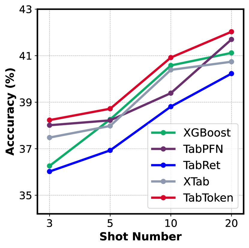
(a) Eye (medium).

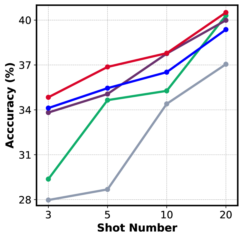
(b) Jannis (medium).

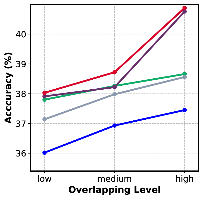
(c) Eye (5shot).

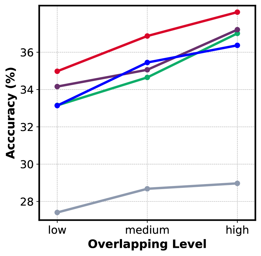
(d) Jannis (5shot).

Figure 6: Results for different shots and overlapping ratios. TabToken outperforms other baselines with different degrees of data limitations. When the overlapping feature ratio improves, TabToken can leverage a larger proportion of pre-trained feature tokens, leading to improved performance.

Different Shots and Overlapping Ratios. In order to fully verify the robustness of TabToken, we conduct experiments on $\{3,5,10,20\}$-shot and adjust the overlapping ratio to three levels {low, medium, high}.  Figure 6 shows that TabToken can maintain the transfer effect in different shots and overlapping ratios. The specific number of features for different overlapping ratios is in Table 5.

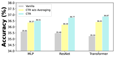
Figure 7: The results of 5-shot downstream tasks in Jannis. “Vanilla” means transferring feature tokens obtained by vanilla pre-training.

Different Top-layer Model Types. In the pre-training process, we combine the tokenizer with different top-layer models, and transfer the pre-trained feature tokens to a new transformer for the downstream task. We report the results of different pre-training strategies and pre-trained model types: {MLP, ResNet, Transformer}. We use transformer as the top-layer model in the downstream tasks. Figure 7 shows that even when the pre-training and downstream model types are different , the feature tokens trained with CTR gain transferability. Averaging also plays a role in TabToken.

Table 2: We investigate the ability of TabToken in standard tasks. We train deep models on the full pre-training data. TabToken improves different deep models with either numerical or categorical features. (↑ ~ accuracy).

	Eye↑	Colon↑	Clave↑	Cardio↑	Jannis↑	Htru↑	Breast↑
MLP	0.4633	0.6299	0.7345	0.7317	0.5210	0.9801	0.8855
+ CTR	0.4849	0.6222	0.7412	0.7333	0.5373	0.9823	0.8772
ResNet	0.4670	0.6206	0.7310	0.7318	0.5124	0.9779	0.8771
+ CTR	0.4725	0.6222	0.7326	0.7340	0.5195	0.9803	0.8783
Trans.	0.4638	0.6414	0.7375	0.7325	0.5052	0.9807	0.8686
+ CTR	0.4698	0.6448	0.7467	0.7366	0.5215	0.9813	0.8804

6.2 Token Matters in Improving Deep Models

We investigate whether the token-based deep model can be improved through CTR. We directly evaluate the deep models in the full pre-training dataset. We use Optuna [3] library and search hyperparameters for 30 iterations on the validation set.  Table 2 shows the mean results over 10 random seeds. Different deep model architectures can achieve better prediction performance by coupling with TabToken. TabToken enhances the discriminative ability of deep models in standard tabular tasks. The results validate the potential of TabToken beyond transfer tasks.

7 Conclusion

Transferring a pre-trained tabular model effectively can enhance the learning of a downstream tabular model and improve its efficiency. In this paper, we propose TabToken to improve the transferability of deep tabular models by addressing the quality of feature tokens, which is a crucial component in various deep tabular models. We introduce a contrastive objective that regularizes the tokens and incorporates feature semantics into the token representations. Experimental results on diverse tabular datasets validate the effectiveness of our approach in bridging the gap between heterogeneous feature sets and improving the performance of deep learning models for tabular data.

We highlight the significance of feature tokens when transferring a pre-trained deep tabular model from a task with overlapping features. Our proposed method, TabToken, focuses on improving the quality of feature tokens and demonstrates strong performance in both cross-feature-set and standard tabular data experiments. The Appendix consists of five sections:

• Appendix A: We demonstrate that the feature tokenizer does not increase the model capacity, which emphasizes the importance of enhancing the quality of tokens.

• Appendix B: We describe the architectures of several top-layer models in tabular deep learning, including MLP, ResNet, and Transformer.

• Appendix C: We provide details on generating synthetic datasets and real-world datasets. We specify how to split the dataset for evaluation.

• Appendix D: Additional experiments are presented, including comparisons with more variants and baselines. We extend our approach to more complex scenarios with different label spaces and non-overlapping features.

• Appendix E: Implementation details of baseline methods and TabToken are provided.

Appendix A The Tokenizer Does Not Increase The Model Capacity

Unlike directly handling input data with a deep neural network, the token-based deep models add another embedding layer, which transforms the raw feature into a set of high-dimensional embeddings. In particular, given a labeled tabular dataset $\mathcal{D}=\{({\bm{x}}_{i},y_{i})\}_{i=1}^{N}$ with $N$ instances (rows in the table), the feature tokenizer maps both categorical and numerical feature value $x_{i,j}$ to a $k$-dimensional vector. One of the main motivations of the feature tokenizer is to replace a sparse feature (e.g., the one-hot coding of a categorical feature) with a dense high-dimensional vector with rich semantic meanings [58, 21, 29, 36, 61, 4]. However, in this section, we analyze the feature tokenizer and show that they cannot increase the capacity of deep tabular models.

Following the same notation in the main text, we denote the $j$-th feature of the data as ${\bm{x}}_{:,j}$. Then we take the classification task as an example and analyze both numerical and categorical features.

Numerical Features. If the $j$-th feature is numerical, then the $j$-th element of an instance ${\bm{x}}_{i}$ is ${\bm{x}}_{i,j}\in\mathbb{R}$. When we classify the label of ${\bm{x}}_{i}$ directly, we learn a classifier $w_{0}\in\mathbb{R}$ for ${\bm{x}}_{i,j}$, which predicts ${\bm{x}}_{i,j}$ with $w^{\top}_{0}\cdot{\bm{x}}_{i,j}$. While based on the feature tokenizer, we allocate a learnable embedding $\bm{E}_{j}\in\mathbb{R}^{1\times k}$ for the feature ${\bm{x}}_{:,j}$, and transform ${\bm{x}}_{i,j}$ with $\hat{{\bm{x}}}_{i,j}={\bm{x}}_{i,j}\cdot\bm{E}_{j}\in\mathbb{R}^{1\times k}$. Based on the tokenized numerical feature $\hat{{\bm{x}}}_{i,j}$, the classifier becomes a vector $\bm{w}\in\mathbb{R}^{k}$, and the prediction works as follows:

$$f({\bm{x}}_{i,j})=\bm{w}^{\top}({\bm{x}}_{i,j}\cdot\bm{E}_{j})^{\top}=(\bm{w}^{\top}\bm{E}_{j}^{\top})\cdot{\bm{x}}_{i,j}={w^{\prime}}^{\top}\cdot{\bm{x}}_{i,j},$$

where ${w^{\prime}}^{\top}=\bm{w}^{\top}\bm{E}_{j}^{\top}\in\mathbb{R}$. Therefore, it has the same effect as the original learning approach $w_{0}$.

Categorical Features. If the $j$-th feature is categorical with $K_{j}$ choices, we rewrite ${\bm{x}}_{i,j}$ in the one-hot coding form, i.e., ${\bm{x}}_{i,j}\in\{0,1\}^{K_{j}}\in\mathbb{R}^{K_{j}}$. Assume the classifier for the one-hot feature is $\bm{\eta}_{0}\in\mathbb{R}^{K_{j}}$, which predicts ${\bm{x}}_{i,j}$ with $\bm{\eta}_{0}^{\top}{\bm{x}}_{i,j}$. The tokenizer for a categorical feature works as a lookup table. Given $\bm{E}_{j}=\{\bm{e}_{p}\}_{p=1}^{K_{j}}\in\mathbb{R}^{K_{j}\times k}$ is the set of candidate tokens for the $j$-th feature, then we have $\hat{{\bm{x}}}_{i,j}={\bm{x}}_{i,j}^{\top}\bm{E}_{j}\in\mathbb{R}^{1\times k}$, which selects the corresponding token based on the index of the categorical feature value set. The classifier for the tokenized feature is $\bm{\eta}\in\mathbb{R}^{k}$ and the prediction is:

$$f({\bm{x}}_{i,j})=\bm{\eta}^{\top}({\bm{x}}_{i,j}^{\top}\bm{E}_{j})^{\top}=\bm{\eta}^{\top}\bm{E}_{j}^{\top}{\bm{x}}_{i,j}=\left[\bm{\eta}^{\top}\bm{e}_{1},\bm{\eta}^{\top}\bm{e}_{2},\ldots,\bm{\eta}^{\top}\bm{e}_{K_{j}}\right]{\bm{x}}_{i,j}={\bm{\eta}^{\prime}}^{\top}{\bm{x}}_{i,j},$$

where ${\bm{\eta}^{\prime}}^{\top}=\left[\bm{\eta}^{\top}\bm{e}_{1},\bm{\eta}^{\top}\bm{e}_{2},\ldots,\bm{\eta}^{\top}\bm{e}_{K_{j}}\right]\in\mathbb{R}^{1\times K_{j}}$. Therefore, the representation ability of the token-based model is the same as the original one $\bm{\eta}_{0}$.

Summary. The feature tokenizer does not increase the model capacity. Training with feature tokens cannot automatically associate the feature semantics with the tokens. Therefore, we incorporate the feature semantics into the tokens with a contrastive regularization in TabToken, which makes the learned tokens facilitate the reuse of tabular deep models across feature sets.

Appendix B Top-layer Models

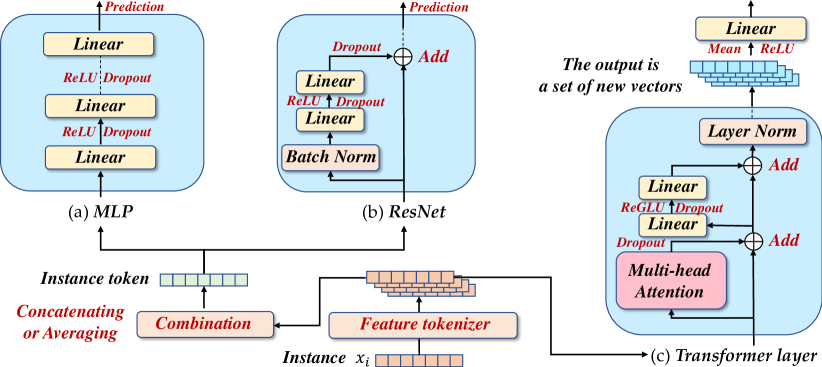
Figure 8: The feature tokenizer and top-layer models. (a) The Multi-Layer Perceptron needs the feature combination to process the input set of vectors. (b) The same to MLP, the Residual Network needs the feature combination to utilize a feature tokenizer. (c) A set of vectors can feed into the Transformer layer directly. The output is also a set of vectors, different from using a class token, we take the average of these vectors to obtain the vector used for the final prediction.

Based on the transformed tokens, deep tabular models implement the classifier with various top-layer models, e.g., MLP, ResNet, and Transformer. In this section, we formally describe the details of these models, whose architectures mainly follow the designs in [18]. However, instead of applying MLP and ResNet on raw features, we treat MLP and ResNet as the top-layer model upon the feature tokenizer. It is notable that the output of the feature tokenizer is a set of vectors. The main procedure is illustrated in  Figure 8.

B.1 MLP

Given a set of tokens, we transform them into a vector via token averaging or concatenating as described in the main text. With a bit of abuse of notation, we denote the processed token as ${\bm{x}}$, whose dimension is $k$ or $dk$ when we average or concatenate the tokens, respectively. The MLP architecture is designed as follows based on ${\bm{x}}$:

$${\rm MLP}({\bm{x}}) ={\rm Linear}({\rm MLPBlock}(\ldots({\rm MLPBlock}({\bm{x}}))),$$

$${\rm MLPBlock}({\bm{x}}) ={\rm Dropout}({\rm ReLU}({\rm Linear}({\bm{x}}))),$$

where ${\rm Linear(\cdot)}$ is a fully connected layer, which performs a linear transformation on the input data by applying a matrix multiplication followed by an optional bias addition. ${\rm Dropout(\cdot)}$ is a regularization technique, which works by randomly deactivating a certain percentage of neurons during each training step. ${\rm ReLU(\cdot)}$ is a simple and computationally efficient non-linear function that introduces non-linearity into the networks.

B.2 ResNet

The same as MLP, we employ ResNet on the feature tokens, and the architecture is:

$${\rm ResNet}({\bm{x}}) ={\rm Prediction}\left({\rm ResNetBlock}\left(\ldots\left({\rm ResNetBlock}\left({\rm Linear}({\bm{x}})\right)\right)\right)\right),$$

$${\rm ResNetBlock}({\bm{x}}) ={\bm{x}}+{\rm Dropout}({\rm Linear}({\rm Dropout}({\rm ReLU}({\rm Linear}({\rm BatchNorm}({\bm{x}})))))),$$

$${\rm Prediction}({\bm{x}}) ={\rm Linear}\left({\rm ReLU}\left({\rm BatchNorm}\left({\bm{x}}\right)\right)\right),$$

where ${\rm BatchNorm(\cdot)}$ is a technique used in neural networks during training [30]. ${\rm BatchNorm(\cdot)}$ normalizes the activations of a specific layer by adjusting and scaling them based on the statistics of the mini-batch.

B.3 Transformer

Different from MLP or ResNet, Transformer processes the set of tokens simultaneously, and the output of Transformer is a set of tokens with the same form as the input one. Assume the input matrix $\bm{X}$ is the set of $k$-dimensional vectors $\bm{X}\in\mathbb{R}^{d\times k}$, the general prediction flow of Transformer-based deep tabular model is:

$${\rm Transformer}(\bm{X}) ={\rm Prediction}({\rm TransformerLayer}(\ldots({\rm TransformerLayer}(\bm{X})))),$$

$${\rm Prediction}(\bm{X}) ={\rm Linear}({\rm ReLU}({\rm mean}(\bm{X}))),$$

where the Transformer layer is implemented as

$${\rm TransformerLayer}(\bm{X}) ={\rm LayerNorm}({\rm Residual}({\rm FFN},\ {\rm Residual}({\rm MultiheadAttention},\bm{X}))),$$

$${\rm Residual}({\rm Module},\bm{X}) =\bm{X}+{\rm Dropout}({\rm Module}(\bm{X})),$$

$${\rm FFN}(\bm{X}) ={\rm Linear}({\rm Dropout}({\rm ReGLU}({\rm Linear}(\bm{X})))),$$

where ${\rm LayerNorm(\cdot)}$ is a normalization layer that performs layer normalization on the input [7]. It computes the mean and standard deviation along specified axes and normalizes the tensor using these statistics. It is an alternative to ${\rm BatchNorm(\cdot)}$ and is commonly used in Transformer where batch statistics are inappropriate. ${\rm MultiheadAttention(\cdot)}$ is a key component of Transformer-based architectures, allowing the model to attend to multiple parts of the input sequence simultaneously and capture diverse patterns and relationships. $\rm ReGLU(\cdot)$ is a GLU variant designed for Transformer [44].

Appendix C Data

In this section, we introduce the detailed properties of source datasets and describe how to construct the synthetic datasets. We also introduce how to split real-world datasets into heterogeneous pre-training and fine-tuning datasets.

C.1 Data Preprocessing

For the sake of fair comparison, almost identical preprocessing steps are applied to all methods. In the case of categorical datasets, missing values are treated as a new discrete choice within each feature. As for numerical datasets, missing values are filled with the mean value of each respective feature. Standardization, involving mean subtraction and scaling, is applied to normalize each numerical dataset. To handle categorical features, encoding methods are employed to assist baselines that lack direct support. In the case of TabPFN [25], an ordinal encoder is utilized to ensure a limited quantity of encoded features for the method to work well on gpu. For other baselines, one-hot encoding is employed when necessary.

C.2 Synthetic Datasets

We aim to construct a synthetic four-class classification dataset with semantically similar features and random features. As described in the main text, the dataset consists of six features $\{x_{:,i}\}_{i=1}^{6}$, each feature with four categorical choices. When constructing each sample in the dataset, the feature value is as follows ($p$ is the probability) :

• $x_{:,1}\in\{A,B,C,D\}$, $p=0.25$ is assigned to each choice.

• $x_{:,2}\in\{E,F,G,H\}$, $p=0.25$ is assigned to each choice.

• $x_{:,3}\in\{A^{\prime},B^{\prime},C^{\prime},D^{\prime}\}$, $x_{:,3}=x_{:,1}$ with $p=0.8$; random choices otherwise.

• $x_{:,4}\in\{E^{\prime},F^{\prime},G^{\prime},H^{\prime}\}$, $x_{:,4}=x_{:,2}$ with $p=0.8$; random choices otherwise.

• $x_{:,5}$ and $x_{:,6}$ are comletely random choices.

The label $y\in\{1,2,3,4\}$ of a sample is assigned following the rules:

• when $x_{:,1}\in\{C,D\}$ and $x_{:,2}\in\{E,F\}$, $y=1$ with $p=0.8$; random choices otherwise.

• when $x_{:,1}\in\{A,B\}$ and $x_{:,2}\in\{G,H\}$, $y=2$ with $p=0.8$; random choices otherwise.

• when $x_{:,1}\in\{A,B\}$ and $x_{:,2}\in\{E,F\}$, $y=3$ with $p=0.8$; random choices otherwise.

• when $x_{:,1}\in\{C,D\}$ and $x_{:,2}\in\{G,H\}$, $y=4$ with $p=0.8$; random choices otherwise.

It is clearly shown in the rules of construction that, within 80% probability, $x_{:,1}$ and $x_{:,3}$, $x_{:,2}$ and $x_{:,4}$ have a one-to-one correspondence with the categorical choices, they are semantically similar features, while $x_{:,5}$ and $x_{:,6}$ are random noise features. We expect the feature tokens of $A^{\prime}$ to be close to $A$, $B^{\prime}$ close to $B$, ${\it etc}$. Besides, we aim at identifying the random features $x_{:,5}$ and $x_{:,6}$ from the feature tokens. As demonstrated in the main text, TabToken incorporates these semantics into the feature tokens, fulfilling our aforementioned objectives.

Table 3: Descriptions of full datasets. There are different feature types and task types. These full datasets will be divided into pre-training datasets and fine-tuning datasets.

Properties Eye Colon Clave Cardio Jannis Htru Breast Elevators Super Volume Feature type num cat cat num num num cat num num num Feature num 26 18 16 11 54 8 29 18 81 53 Task type multiclass binary multiclass binary multiclass binary binary regression regression regression Size of full 10.9K 3.0K 10.8K 70.0K 83.7K 17.9K 3.9K 16.6K 21.3K 50.9K Size of train 7.0K 1.8K 6.9K 44.8K 53.6K 11.5K 2.3K 10.6K 13.6K 32.8K Size of val 1.8K 0.6K 1.7K 11.2K 13.4K 2.9K 0.8K 2.7K 3.4K 8.1K Size of test 2.2K 0.6K 2.2K 14.0K 16.7K 3.6K 0.8K 3.3K 4.3K 10.0K Source OpenML Datasphere UCI Kaggle AutoML UCI Datasphere OpenML UCI UCI

C.3 Real-world Datasets and evaluation setups

To get datasets in different domains, the real-world datasets are from OpenML [50], UCI, AutoML, Kaggle, and Projectdatasphere. The descriptions are shown in Table 3.

Table 4: Descriptions of transferring datasets and fine-tuning datasets. We maintain an overlap of approximately 50% between the overlapping features and the fine-tuning features, which corresponds to the “medium” level among different overlapping ratios. “# Pre-training feature” denotes the number of pre-training features.

Properties Eye Colon Clave Cardio Jannis Htru Breast Elevators Super Volume # Pre-training feature 17 13 11 7 36 6 20 12 54 35 # Fine-tuning feature 17 12 10 7 36 5 19 12 54 35 # Overlapping feature 8 7 5 3 38 3 10 6 27 17

We randomly sample 20% instances to construct the test set. In the remaining dataset, we randomly hold out 20% instances as the validation set. We split the final training set into two parts. The first part consists of 80% training instances, which are utilized as pre-training dataset. The remaining instances are used for sampling few-shot downstream datasets. The validation set is only used in the pre-training stage for saving the best checkpoint as the pre-training model.

To obtain a clearer explanation, consider a tabular dataset with nine features: f1 to f9. The upstream dataset comprises features f1 to f6, while the downstream dataset includes features f4 to f9. The details of transferring dataset are shown in  Table 4.

Table 5: Different overlapping ratios of transferring datasets. (l: low, m: medium, h: high). The overlapping ratios are calculated by dividing “# Overlapping feature” by “# Fine-tuning feature”.

Properties	Jannis (l)	Jannis (m)	Jannis (h)	Eye (l)	Eye (m)	Eye (h)
# Pre-training feature	34	36	38	16	17	19
# Fine-tuning feature	34	36	38	15	17	18
# Overlapping feature	14	18	22	5	8	11
Overlapping ratio (%)	41	50	69	33	47	61

(1) The number of shots is the sample size for each class. For instance, a 5-shot dataset for binary classification consists of $5\times 2$ samples. (2) The overlapping ratio is defined as the ratio between the number of overlapping features and the total number of features used for fine-tuning. The low, medium, and high overlapping ratios are shown in  Table 5. In the main text, we investigate the cases with different number of shots or different overlapping ratios.

Appendix D Additional Analyses and Experiments

We analyze TabToken from various aspects. First, we investigate several possible implementations of “Contrastive Token Regularization (CTR)”, and demonstrate that the simple contrastive form in the main text works the best. Then in  subsection D.2, we test the ability of TabToken when the target data share the same feature space but different distributions with the pre-trained model. We also explore the variant of TabToken when the target data have entirely different feature and label spaces with the pre-trained model.

D.1 Additional Analyses and Comparisons

Table 6: The whole results in Table 1. $\dagger$: TabPFN does not support regression tasks. ( ↑ ~ accuracy, ↓ ~ RMSE).

Eye↑ Colon↑ Clave↑ Cardio↑ Jannis↑ Htru↑ Breast↑ Elevators↓ Super↓ Volume↓ SVM 0.3621 0.5921 0.3482 0.6036 0.3512 0.8376 0.8211 0.0088 33.9036 124.2391  $\pm$ 0.0044  $\pm$ 0.0028  $\pm$ 0.0094  $\pm$ 0.0027  $\pm$ 0.0048  $\pm$ 0.0029  $\pm$ 0.0049  $\pm$ 0.0003  $\pm$ 1.0362  $\pm$ 1.3914 XGBoost 0.3699 0.5676 0.3506 0.5703 0.3222 0.8369 0.8453 0.0090 34.6605 123.9724  $\pm$ 0.0035  $\pm$ 0.0074  $\pm$ 0.0027  $\pm$ 0.0047  $\pm$ 0.0063  $\pm$ 0.0028  $\pm$ 0.0092  $\pm$ 0.0002  $\pm$ 1.7548  $\pm$ 1.6470 FT-trans 0.3916 0.5792 0.3584 0.6064 0.3064 0.8252 0.8275 0.0081 31.3274 122.8319  $\pm$ 0.0075  $\pm$ 0.0028  $\pm$ 0.0083  $\pm$ 0.0013  $\pm$ 0.0047  $\pm$ 0.0028  $\pm$ 0.0018  $\pm$ 0.0003  $\pm$ 0.9462  $\pm$ 1.0277 TabPFN^† 0.3918 0.5809 0.3733 0.5965 0.3601 0.8371 0.7438 - - -  $\pm$ 0.0064  $\pm$ 0.0082  $\pm$ 0.0016  $\pm$ 0.0037  $\pm$ 0.0045  $\pm$ 0.0027  $\pm$ 0.0029 SCARF 0.3371 0.6048 0.2144 0.5547 0.3523 0.8131 0.7063 0.0097 39.9343 124.5373  $\pm$ 0.0125  $\pm$ 0.0152  $\pm$ 0.0127  $\pm$ 0.0094  $\pm$ 0.0081  $\pm$ 0.0058  $\pm$ 0.0083  $\pm$ 0.0004  $\pm$ 1.4749  $\pm$ 2.1749 TabRet 0.3477 0.4688 0.2393 0.4329 0.3545 0.8231 0.7252 0.0094 41.2537 126.4713  $\pm$ 0.0017  $\pm$ 0.0048  $\pm$ 0.0082  $\pm$ 0.0038  $\pm$ 0.0037  $\pm$ 0.0037  $\pm$ 0.0085  $\pm$ 0.0002  $\pm$ 1.4772  $\pm$ 1,2734 XTab 0.3851 0.5964 0.3627 0.5856 0.2868 0.8363 0.8145 0.0077 38.5030 119.6656  $\pm$ 0.0085  $\pm$ 0.0045  $\pm$ 0.0074  $\pm$ 0.0047  $\pm$ 0.0092  $\pm$ 0.0037  $\pm$ 0.0019  $\pm$ 0.0002  $\pm$ 1.7463  $\pm$ 0.8743 ORCA 0.3823 0.5876 0.3689 0.6042 0.3413 0.8421 0.8242 0.0082 37.9436 121.4952  $\pm$ 0.0037  $\pm$ 0.0074  $\pm$ 0.0018  $\pm$ 0.0041  $\pm$ 0.0082  $\pm$ 0.0048  $\pm$ 0.0054  $\pm$ 0.0003  $\pm$ 2.1852  $\pm$ 1.2876 TabToken 0.3982 0.6074 0.3741 0.6229 0.3687 0.8459 0.8284 0.0074 30.9636 118.7280  $\pm$ 0.0054  $\pm$ 0.0061  $\pm$ 0.0023  $\pm$ 0.0024  $\pm$ 0.0015  $\pm$ 0.0034  $\pm$ 0.0013  $\pm$ 0.0002  $\pm$ 1.5274  $\pm$ 1.0285

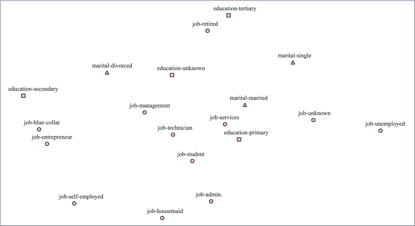
Figure 9: Feature tokens with vanilla training on bank-marketing dataset.

Visualization of feature tokens with vanilla training on bank-marketing dataset. As shown in Figure 9, withour our CTR, the distribution of feature tokens is random.

Different Forms of Contrastive Token Regularization. In CTR, we aim to incorporate the semantics of features into tokens. One main intuition is that the tokens with similar feature semantics should be close while those tokens corresponding to different features may be far away from each other. Given a target dataset $\mathcal{D}^{t}=\{({\bm{x}}_{i}^{t},y_{i}^{t})\}_{i=1}^{N^{t}}$ with $N^{t}$ examples and $d_{t}$ features, the feature tokenizer $h$ and feature combination (averaging or concatenating) process instance ${\bm{x}}_{i}^{t}$ to instance token $\bm{T}_{i}$. Assume there are $C$ classes in total, we denote the class center belonging to the target label $y_{i}$ of instance ${\bm{x}}_{i}^{t}$ as $\bm{S}_{y_{i}}$, while the class centers of different labels as $\bm{S}_{j\neq y_{i}}$. Recall that $h$ is the feature tokenizer and $g$ is the top-layer model. The CTR is usually optimized with the following objective:

$$\min_{h,g}\sum_{i=1}^{N^{t}}\left[\ell(g\circ h({\bm{x}}^{t}_{i}),y^{t}_{i})\right]+\beta\Omega\left(\{\bm{T}_{i}\}_{i=1}^{N^{t}}\right).$$

Here are possible implementations of the token regularization $\Omega$:

• Vanilla CTR: the implementation that we used in TabToken, which minimizes the distance between an instance token with its target class center:

  $$\Omega_{{\rm{\sc TabToken}}}\left(\{\bm{T}_{i}\}_{i=1}^{N^{t}}\right)=\frac{1}{N^{t}}\sum_{i=1}^{N^{t}}\left\|\bm{T}_{i}-\bm{S}_{y_{i}}\right\|^{2}_{2}.$$

• Hardest: the objective is to push $\bm{T}_{i}$ away from the nearest center of the different classes, which aims at moving instances away from the centers of the most easily misclassified labels.

  $$\Omega_{{\rm hardest}}\left(\{\bm{T}_{i}\}_{i=1}^{N^{t}}\right)=\frac{1}{N^{t}}\sum_{i=1}^{N^{t}}{\rm min}(\{\left\|\bm{T}_{i}-\bm{S}_{j}\right\|^{2}_{2}\}_{j\neq y_{i}}).$$

• All-hard: the objective is to push $\bm{T}_{i}$ away from all the centers of the different classes, which minimize the average distance between the instance and the centers of all other labels. (while in the binary classification task and regression task, “All-hard” and “Hardest” are the same).

  $$\Omega_{{\rm all-hard}}\left(\{\bm{T}_{i}\}_{i=1}^{N}\right)=\frac{1}{{N^{t}}\cdot(C-1)}\sum_{i=1}^{N^{t}}\sum_{j\neq y_{i}}(\left\|\bm{T}_{i}-\bm{S}_{j}\right\|^{2}_{2}).$$

• Supcon: the supervised contrastive loss [33]. The objective remains the same, which is to bring instances of the same label closer together while keeping instances of different labels far apart. However, this approach requires more calculations based on the distances of instance tokens. We use the default configuration of official implementation.

• Triplet: the triplet contrastive loss with margin [24]. The objective is to ensure that the positive examples are closer to the anchor than the negative examples by at least the specified margin. We use the default configuration of official implementation.

• TabToken + hard: the objective is the combination of CTR and All-hard:

  $$\Omega_{{\rm{\sc TabToken}+hard}}=\frac{1}{{N^{t}}}\sum_{i=1}^{N^{t}}\left(\left\|\bm{T}_{i}-\bm{S}_{y_{i}}\right\|^{2}_{2}-\frac{1}{C-1}\sum_{j\neq y_{i}}\left\|\bm{T}_{i}-\bm{S}_{j}\right\|^{2}_{2}\right).$$

Table 7: Test accuracy on fine-tuning datasets for different forms of contrastive token regularization. We use TabToken with different token regularization techniques on the pre-training dataset. We reuse the pre-trained feature tokenizer and apply token regularization during fine-tuning on the 5-shot downstream dataset. TabToken is considered better overall, but in certain cases such as Jannis and Htru, further improvement can be achieved by incorporating another token regularization that focuses on pushing apart the centers of different classes. (↑ ~ accuracy, ↓ ~ RMSE).

Eye↑ Colon↑ Clave↑ Cardio↑ Jannis↑ Htru↑ Breast↑ Elevators↓ Super↓ Volume↓ $\Omega_{{\rm hardest}}$ 0.3803 0.5895 0.3577 0.6155 0.3462 0.8422 0.8121 0.0083 35.8297 121.2847 $\Omega_{{\rm all-hard}}$ 0.3792 0.5895 0.3596 0.6155 0.3483 0.8422 0.8121 0.0083 35.8297 121.2847 $\Omega_{{\rm supcon}}$ 0.3904 0.5976 0.3701 0.6041 0.3204 0.8293 0.8233 0.0077 34.8366 119.9927 $\Omega_{{\rm triplet}}$ 0.3993 0.5983 0.3675 0.6055 0.3049 0.8431 0.8178 0.0082 33.1726 120.8255 $\Omega_{{\rm{\sc TabToken}}}$ 0.3982 0.6074 0.3741 0.6229 0.3687 0.8459 0.8284 0.0074 30.9636 118.7280 $\Omega_{{\rm{\sc TabToken}}+{\rm hard}}$ 0.3911 0.6032 0.3678 0.6204 0.3936 0.8625 0.8253 0.0076 32.1836 118.7364

We use TabToken with different token regularization techniques. We reuse the pre-trained feature tokenizer and apply token regularization during fine-tuning on the 5-shot downstream dataset. The results in the  Table 7 shows the test accuracy for downstream tasks with 5-shot. The same to the evaluation in the main text, for each method and dataset, we train on 30 randomly sampled few-shot subsets, reporting the performance averaged over 10 random seeds. The only difference in training is the type of token regularization. Although $\Omega_{{\rm{\sc TabToken}}}$ is the simplest objective, it allows the feature tokens of the pre-trained model to obtain better transferability.

Table 8: Test accuracy of different methods on the 5-shot fine-tuning datasets with the help of pre-training. The construction of transferring datasets is shown in  Table 4. Token loss allows tokens to gain potential for prediction, but the transferability of feature tokens is not as strong as in TabToken. OPID, by utilizing model ensemble, has achieved better performance on Jannis and Htru. TabToken shows superior performance on most datasets. (↑ ~ accuracy, ↓ ~ RMSE).

	Eye↑	Colon↑	Clave↑	Cardio↑	Jannis↑	Htru↑	Breast↑
Token head	0.3863	0.6058	0.3683	0.6225	0.3675	0.8497	0.8059
LR transfer	0.3661	0.6001	0.3561	0.5947	0.3552	0.6834	0.7817
OPID	0.3903	0.5942	0.3689	0.6091	0.3754	0.8784	0.8143
TabToken	0.3982	0.6074	0.3741	0.6229	0.3687	0.8459	0.8284

Different Methods for Feature Overlapping. We compare baselines suitable for overlapping features, the descriptions are as follows:

• “Token loss” simultaneously train a linear classifier on the instance tokens during the training process of TabToken and incorporating its loss into the final loss instead of CTR, the quality of feature tokens is expected to be improved by direct predicting based on the tokens.

• In “LR transfer”, the logistic regression classifier obtained from the pre-training set is directly used to initialize the fine-tuning classifier with the overlapping part. For features that are unseen in the fine-tuning phase, their corresponding weights are initialized to zero.

• In “OPID” [28], during the pre-training phase, a sub-classifier is jointly trained on overlapping features, and the output of this sub-classifier is treated as knowledge from the pre-training set. This knowledge, in the form of new features, is concatenated with the fine-tuning dataset. During the fine-tuning phase, the sub-classifier and the new classifier are jointly trained, and the final prediction is the weighted sum of their predictions.

The results for these three baselines are in  Table 8. Although OPID shows advantages in two datasets, when pre-training, it need the information about which features will be overlapping features in downstream task. While all features are treated equally during pre-training in TabToken. Besides, OPID benefits from the ensemble of classifiers.

Table 9: Test accuracy on the 5-shot fine-tuning datasets when the instance distributions are changed. (SD: same distribution, DD: different distributions). We add Gaussian noise to pre-training datasets to change the instance distributions. $\Delta$ is the average absolute change in prediction accuracy for the three methods when there is a distribution shift across five datasets. TabToken can maintain its transferability and significantly outperform the other two transfer methods.

	Eye	Cardio	Jannis	Htru	$\Delta$
SCARF (SD)	0.3371	0.5547	0.3523	0.5938	0.0288
SCARF (DD)	0.3561	0.5320	0.3547	0.4958
TabRet(SD)	0.3477	0.4329	0.3545	0.6305	0.0484
TabRet (DD)	0.3661	0.5063	0.3189	0.5175
TabToken (SD)	0.3982	0.6229	0.3678	0.8459	0.0037
TabToken (DD)	0.3989	0.6189	0.3629	0.8479

D.2 Extension to More Complex Scenarios

Different Instance Distributions. To explore the scenario where the feature space is the same, but the pre-training instance distribution differs from the fine-tuning distribution, we first split the full training set into two halves. In the first part, we construct the pre-training dataset by adding Gaussian noise. The standard deviation of noise is 10% of the feature’s standard deviation. In the second part, we extract thirty 5-shot sub-datasets as downstream tasks. To facilitate the addition of Gaussian noise, we conduct experiments on numerical datasets. The results are in  Table 9. TabToken is robust to the deviation of instance distributions, achieving the least changes in prediction performance.

Different Feature and Label Space. We explore transferring scenarios where the pre-training dataset and fine-tuning dataset are completely different. We use CTR to pre-train transformer on Jannis, which owns a large number of features. We expect the downstream task to select feature tokens from these completely non-overlapping but semantically meaningful tokens using a re-weighting mechanism. By incorporating $n$ learnable new feature tokens $\{\bm{E}_{j}^{\textit{\rm new}}\}_{j=1}^{n}$ and a matching layer $\bm{W}\in\mathbb{R}^{d_{t}\times(d+n)}$, we adapt TabToken for scenarios with non-overlapping features.

Table 10: Test accuracy for different feature and label space. We conduct experiments on 5-shot Eye datasets with different feature numbers. We pre-train feature tokenizer with transformer on full Jannis, fine-tuning on 30 randomly sampled few-shot subsets. re-weighting based TabToken can benefit from pre-trained feature tokens, especially when the number of fine-tuning features is not large.

	Eye (l)	Eye (m)	Eye (h)
XGBoost	0.3719	0.3699	0.3909
CatBoost	0.3759	0.3791	0.3974
FT-trans	0.3857	0.3916	0.3922
TabPFN	0.3885	0.3918	0.4081
TabToken	0.3923	0.3977	0.3974

We concatenate the new tokens with $d$ pre-trained feature tokens, constructing a “token library” $\left(\{\bm{E}_{j}^{\textit{\rm pre}}\}_{j=1}^{d}\cup\{\bm{E}_{j}^{\textit{\rm new}}\}_{j=1}^{n}\right)\in\mathbb{R}^{(d+n)\times k}$. The expression for re-weighting based TabToken is as follows:

$$\{\bm{E}_{j}^{\textit{\rm fine}}\}_{j=1}^{d_{t}}=\bm{W}\left(\{\bm{E}_{j}^{\textit{\rm pre}}\}_{j=1}^{d}\cup\{\bm{E}_{j}^{\textit{\rm new}}\}_{j=1}^{n}\right)\in\mathbb{R}^{d_{t}\times k}.$$

where $\{\bm{E}_{j}^{\textit{\rm fine}}\}_{j=1}^{d_{t}}$ is the feature tokens for fine-tuning feature tokenizer $h$, $\{\bm{E}_{j}^{\textit{\rm pre}}\}_{j=1}^{d}$ is the pre-trained feature tokens of $h_{0}$. $\bm{W}$ is the re-weighting matrix for selecting feature tokens.

Overlapping feature transfer methods like TabRet may not be suitable for scenarios where there are non-overlapping features. TabToken constructs a feature tokenizer by re-weighting the feature tokens in the pre-training set. We expect to obtain more useful feature tokens by training fewer parameters.  Table 10 reports the performance with different number of fine-tuning features. Despite the disparity between the pre-training and the fine-tuning dataset, re-weighting is a token search-like mechanism to enable the target task to benefit from the heterogeneous pre-trained feature tokens.

Summary. Among various contrastive token regularizations, simple CTR has demonstrated superior performance in transferring tasks. Compared to other methods, TabToken is capable of obtaining easily transferable feature tokens during the pre-training phase. TabToken maintains its transferability even when there are differences in instance distributions. Re-weighting based TabToken proves to be effective when there is a non-overlapping feature set.

D.3 Ablation study

We first adjust the modules tuned during the transfer process. Then, we conduct an ablation study based on different pre-training data sizes and token dimensions.

Table 11: Test accuracy for different tuning modules. We pre-train transformer on pre-training datasets as in  Table 4. When we fix certain part of the pre-trained transformer and fine-tune, the pre-training model have lower transferring effect than TabToken. The frozen pre-trained top-layer model is not suitable for overlapping transfer scenarios. Feature tokens with semantics should be used for transfer. The best choice is to directly fine-tune the entire top-layer model as TabToken.

	Eye	Cardio
Tune last layer	0.3907	0.6155
Tune attention	0.3894	0.6217
Tune linear	0.3886	0.6153
Fix top-layer	0.3770	0.5983
TabToken	0.3982	0.6229

Tuning Modules. In TabToken, we do not fix the top-layer model when fine-tuning, while tuning all the transformer, which indicates that feature tokens matter. We compare various tuning choices. When we train the fine-tuning tokenizer using TabToken, we tune the last ${\rm TransformerLayer}(\cdot)$, tune the ${\rm MultiheadAttention}(\cdot)$, and tune the ${\rm Linear}(\cdot)$ in Transformer layer while keeping other modules in Transformer frozen (the final prediction linear head is trainable). Besides, we conduct experiments on tuning the entire fine-tuning tokenizer with fixed top-layer model. The results in  Table 11 show that token matters in transferring, we need to tune the entire top-layer model.

Table 12: Test accuracy for different token dimension and pre-training size. Left: The influence of token dimension. We change the dimension of feature tokens in tokenizer. We find that increasing the dimension of tokens does not lead to better transfer effect. Right: The transferring results with different size of pre-training dataset. We sample subsets from the pre-training dataset based on different proportions. TabToken does not need a large amount of pre-training data to achieve the transfer effect.

	Eye	Cardio
16	0.3909	0.5859
32	0.3999	0.6258
64	0.3982	0.6229
128	0.3977	0.6182
256	0.3949	0.6060

	Eye	Cardio
20%	0.3836	0.6205
40%	0.3878	0.6207
60%	0.3992	0.6179
80%	0.3962	0.6185
100%	0.3982	0.6229

Tuning Token Dimension and Pre-training Size. In our other experiments, we use a default token dimension of 64. Now, we will conduct experiments with token dimensions of 16, 32, 64, 128, and 256. Conventional transfer methods typically require a large amount of pre-training data. In our study, we randomly sample 20%, 40%, 60%, 80%, and 100% of the pre-training dataset to investigate the impact of data volume on the transfer performance of TabToken. The results in  Table 12 show that the larger dimension of tokens is not always better. TabToken exhibits stable transfer performance even when the data volume decreases. TabToken does not need a large amount of pre-training data to achieve the transfer effect.

Appendix E Implementation

In this section, we present the experimental configurations employed for the baselines and TabToken. Given the absence of a validation dataset in the downstream few-shot task, we adopt default configurations to ensure a fair comparison. For standard tabular task, we follow the hyper-parameter space in [18]. All hyper-parameters are selected by Optuna library with Bayesian optimization over 30 trials. The best hyper-parameters are used and the average accuracy over 10 different random seeds is calculated.

MLP and ResNet. We use three-layer MLP and set dropout to 0.2. The feature token size is set to 64 for MLP, ResNet, and Transformer. The default configuration of ResNet is in the left of  Table 13.

Transformer. The right tabular of  Table 13 describes the configuration of FT-trans [18] and Transformer layer in TabToken.

Table 13: The parameters of ResNet and Transformer for top-layer models. Left: Default configuration used for ResNet. Right: Default configuration used for Tranformer which is also the configuration for implementing FT-trans.

Layer count	3
Feature token size	64
Token bias	False
Layer size	168
Hidden factor	2.9
Hidden dropout	0.5
Residual dropout	0.0
Activation	ReLU
Normalization	BatchNorm
Optimizer	AdamW
Pre-train Learning rate	1e-3
Weight decay	2e-4

Layer count	3
Feature token size	64
Token bias	False
Head count	8
Activation & FFN size factor	ReGLU, $\nicefrac{{4}}{{3}}$
Attention dropout	0.08
FFN dropout	0.3
Residual dropout	0.1
Initialization	Kaiming
Optimizer	AdamW
Pre-train Learning rate	1e-3
Fine-Tune Learning rate	5e-4
Weight decay	2e-4

TabPFN. We use the official implementation ( https://github.com/automl/TabPFN) and use the default configuration.

SCARF and TabRet. We use the default configutation in https://github.com/pfnet-research/tabret, which is also the official implementation of TabRet [39]. To ensure a fair comparison, we set the number of pre-training epochs to 200, patience to 20, fine-tuning epochs to 20. We modified the implementations to prevent the use of the validation set during the fine-tuning process.

XTab. We reuse the checkpoint with the highest number (2k) of training epochs from the official implementation of XTab [62] (https://github.com/BingzhaoZhu/XTab). We perform evaluations on the target datasets using XTab’s light fine-tuning approach.

ORCA. We follow the configurations of ORCA [45] for OpenML11 datasets: text for embedder_dataset and roberta for pre-training model. We use the official implementation (https://github.com/sjunhongshen/ORCA).

TabToken. The configuration of feature tokenizer and top-layer models are described in  Table 13. During pre-training, the learning rate is set to 1e-3, the batch size is set to 1024. During fine-tuning, the learning rate is set to 5e-4. We fine-tuning models in 10 epochs.

References

- Addo et al. [2018] Peter Martey Addo, Dominique Guegan, and Bertrand Hassani. Credit risk analysis using machine and deep learning models. Risks, 6(2):38, 2018.
- Ahmed et al. [2010] Nesreen K Ahmed, Amir F Atiya, Neamat El Gayar, and Hisham El-Shishiny. An empirical comparison of machine learning models for time series forecasting. Econometric reviews, 29(5-6):594–621, 2010.
- Akiba et al. [2019] Takuya Akiba, Shotaro Sano, Toshihiko Yanase, Takeru Ohta, and Masanori Koyama. Optuna: A next-generation hyperparameter optimization framework. In Proceedings of the 25th ACM SIGKDD international conference on knowledge discovery & data mining (KDD), 2019.
- Almagor and Hoshen [2022] Chen Almagor and Yedid Hoshen. You say factorization machine, I say neural network - it’s all in the activation. In Proceddings of the 16th ACM Conference on Recommender Systems (RecSys), 2022.
- Arik and Pfister [2021] Sercan Ö. Arik and Tomas Pfister. Tabnet: Attentive interpretable tabular learning. In Proceddings of the 35th AAAI Conference on Artificial Intelligence (AAAI), 2021.
- Awoyemi et al. [2017] John O Awoyemi, Adebayo O Adetunmbi, and Samuel A Oluwadare. Credit card fraud detection using machine learning techniques: A comparative analysis. In 2017 international conference on computing networking and informatics (ICCNI), 2017.
- Ba et al. [2016] Jimmy Lei Ba, Jamie Ryan Kiros, and Geoffrey E Hinton. Layer normalization. arXiv preprint arXiv:1607.06450, 2016.
- Bahri et al. [2022] Dara Bahri, Heinrich Jiang, Yi Tay, and Donald Metzler. Scarf: Self-supervised contrastive learning using random feature corruption. In Proceddings of the 10th International Conference on Learning Representations (ICLR), 2022.
- Beyazit et al. [2019] Ege Beyazit, Jeevithan Alagurajah, and Xindong Wu. Online learning from data streams with varying feature spaces. In Proceedings of the AAAI Conference on Artificial Intelligence (AAAI), 2019.
- Chang et al. [2022] Chun-Hao Chang, Rich Caruana, and Anna Goldenberg. NODE-GAM: neural generalized additive model for interpretable deep learning. In Proceddings of the 10th International Conference on Learning Representations (ICLR), 2022.
- Chen et al. [2022] Jintai Chen, Kuanlun Liao, Yao Wan, Danny Z. Chen, and Jian Wu. Danets: Deep abstract networks for tabular data classification and regression. In Proceddings of the 36th AAAI Conference on Artificial Intelligence (AAAI), 2022.
- Chen and Guestrin [2016] Tianqi Chen and Carlos Guestrin. Xgboost: A scalable tree boosting system. In Proceedings of the 22nd ACM SIGKDD international conference on knowledge discovery & data mining (KDD), 2016.
- Cheng et al. [2016] Heng-Tze Cheng, Levent Koc, Jeremiah Harmsen, Tal Shaked, Tushar Chandra, Hrishi Aradhye, Glen Anderson, Greg Corrado, Wei Chai, Mustafa Ispir, Rohan Anil, Zakaria Haque, Lichan Hong, Vihan Jain, Xiaobing Liu, and Hemal Shah. Wide & deep learning for recommender systems. In Proceedings of the 1st Workshop on Deep Learning for Recommender Systems (DLRS), 2016.
- Devlin et al. [2018] Jacob Devlin, Ming-Wei Chang, Kenton Lee, and Kristina Toutanova. Bert: Pre-training of deep bidirectional transformers for language understanding. arXiv preprint arXiv:1810.04805, 2018.
- Dinh et al. [2022] Tuan Dinh, Yuchen Zeng, Ruisu Zhang, Ziqian Lin, Michael Gira, Shashank Rajput, Jy yong Sohn, Dimitris S. Papailiopoulos, and Kangwook Lee. LIFT: language-interfaced fine-tuning for non-language machine learning tasks. In Advances in Neural Information Processing Systems 35 (NeurIPS), 2022.
- Gando et al. [2016] Gota Gando, Taiga Yamada, Haruhiko Sato, Satoshi Oyama, and Masahito Kurihara. Fine-tuning deep convolutional neural networks for distinguishing illustrations from photographs. Expert Systems with Applications, 66:295–301, 2016.
- Goodfellow et al. [2016] Ian Goodfellow, Yoshua Bengio, and Aaron Courville. Deep learning. MIT press, 2016.
- Gorishniy et al. [2021] Yury Gorishniy, Ivan Rubachev, Valentin Khrulkov, and Artem Babenko. Revisiting deep learning models for tabular data. In Advances in Neural Information Processing Systems 34 (NeurIPS), 2021.
- Gorishniy et al. [2022] Yury Gorishniy, Ivan Rubachev, and Artem Babenko. On embeddings for numerical features in tabular deep learning. In Advances in Neural Information Processing Systems 35 (NeurIPS), 2022.
- Grinsztajn et al. [2022] Léo Grinsztajn, Edouard Oyallon, and Gaël Varoquaux. Why do tree-based models still outperform deep learning on typical tabular data? In Advances in Neural Information Processing Systems 35 (NeurIPS), 2022.
- Guo et al. [2017] Huifeng Guo, Ruiming Tang, Yunming Ye, Zhenguo Li, and Xiuqiang He. Deepfm: A factorization-machine based neural network for CTR prediction. In Proceedings of the Twenty-Sixth International Joint Conference on Artificial Intelligence (IJCAI), 2017.
- Hassan et al. [2020] Md. Rafiul Hassan, Sadiq Al-Insaif, Muhammad Imtiaz Hossain, and Joarder Kamruzzaman. A machine learning approach for prediction of pregnancy outcome following IVF treatment. Neural Computing and Applications, 32(7):2283–2297, 2020.
- Hegselmann et al. [2023] Stefan Hegselmann, Alejandro Buendia, Hunter Lang, Monica Agrawal, Xiaoyi Jiang, and David Sontag. Tabllm: few-shot classification of tabular data with large language models. In International Conference on Artificial Intelligence and Statistics (AISTATS), 2023.
- Hermans et al. [2017] Alexander Hermans, Lucas Beyer, and Bastian Leibe. In defense of the triplet loss for person re-identification. arXiv preprint arXiv:1703.07737, 2017.
- Hollmann et al. [2023] Noah Hollmann, Samuel Müller, Katharina Eggensperger, and Frank Hutter. Tabpfn: A transformer that solves small tabular classification problems in a second. In The Eleventh International Conference on Learning Representations (ICLR), 2023.
- Hou et al. [2021] Bo-Jian Hou, Yu-Hu Yan, Peng Zhao, and Zhi-Hua Zhou. Storage fit learning with feature evolvable streams. In Proceedings of the AAAI Conference on Artificial Intelligence (AAAI), 2021.
- Hou et al. [2022] Bo-Jian Hou, Lijun Zhang, and Zhi-Hua Zhou. Prediction with unpredictable feature evolution. IEEE Transactions on Neural Networks and Learning Systems, 33(10):5706–5715, 2022.
- Hou and Zhou [2018] Chenping Hou and Zhi-Hua Zhou. One-pass learning with incremental and decremental features. IEEE Transactions on pattern analysis and machine intelligence, 40(11):2776–2792, 2018.
- Huang et al. [2020] Xin Huang, Ashish Khetan, Milan Cvitkovic, and Zohar Karnin. Tabtransformer: Tabular data modeling using contextual embeddings. arXiv preprint arXiv:2012.06678, 2020.
- Ioffe and Szegedy [2015] Sergey Ioffe and Christian Szegedy. Batch normalization: Accelerating deep network training by reducing internal covariate shift. In International conference on machine learning (ICML), 2015.
- Katzir et al. [2021] Liran Katzir, Gal Elidan, and Ran El-Yaniv. Net-dnf: Effective deep modeling of tabular data. In Proceedings of the 9th International Conference on Learning Representations (ICLR), 2021.
- Ke et al. [2017] Guolin Ke, Qi Meng, Thomas Finley, Taifeng Wang, Wei Chen, Weidong Ma, Qiwei Ye, and Tie-Yan Liu. Lightgbm: A highly efficient gradient boosting decision tree. In Advances in neural information processing systems 30 (NIPS), 2017.
- Khosla et al. [2020] Prannay Khosla, Piotr Teterwak, Chen Wang, Aaron Sarna, Yonglong Tian, Phillip Isola, Aaron Maschinot, Ce Liu, and Dilip Krishnan. Supervised contrastive learning. In Advances in Neural Information Processing Systems 33 (NeurIPS), 2020.
- Levin et al. [2023] Roman Levin, Valeriia Cherepanova, Avi Schwarzschild, Arpit Bansal, C. Bayan Bruss, Tom Goldstein, Andrew Gordon Wilson, and Micah Goldblum. Transfer learning with deep tabular models. In The Eleventh International Conference on Learning Representations (ICLR), 2023.
- Lim and Zohren [2021] Bryan Lim and Stefan Zohren. Time-series forecasting with deep learning: a survey. Philosophical Transactions of the Royal Society A, 379(2194):20200209, 2021.
- Liu et al. [2021] Siyi Liu, Chen Gao, Yihong Chen, Depeng Jin, and Yong Li. Learnable embedding sizes for recommender systems. In Proceddings of the 9th International Conference on Learning Representations (ICLR), 2021.
- Nederstigt et al. [2014] Lennart J Nederstigt, Steven S Aanen, Damir Vandic, and Flavius Frasincar. Floppies: a framework for large-scale ontology population of product information from tabular data in e-commerce stores. Decision Support Systems, 59:296–311, 2014.
- Nguyen et al. [2012] Hai-Long Nguyen, Yew-Kwong Woon, Wee-Keong Ng, and Li Wan. Heterogeneous ensemble for feature drifts in data streams. In Advances in Knowledge Discovery and Data Mining: 16th Pacific-Asia Conference (PAKDD), 2012.
- Onishi et al. [2023] Soma Onishi, Kenta Oono, and Kohei Hayashi. Tabret: Pre-training transformer-based tabular models for unseen columns. arXiv preprint arXiv:2303.15747, 2023.
- Otter et al. [2020] Daniel W Otter, Julian R Medina, and Jugal K Kalita. A survey of the usages of deep learning for natural language processing. IEEE transactions on neural networks and learning systems, 32(2):604–624, 2020.
- Popov et al. [2020] Sergei Popov, Stanislav Morozov, and Artem Babenko. Neural oblivious decision ensembles for deep learning on tabular data. In Proceddings of the 8th International Conference on Learning Representations (ICLR), 2020.
- Prokhorenkova et al. [2018] Liudmila Ostroumova Prokhorenkova, Gleb Gusev, Aleksandr Vorobev, Anna Veronika Dorogush, and Andrey Gulin. Catboost: unbiased boosting with categorical features. In Advances in Neural Information Processing Systems 31 (NeurIPS), 2018.
- Richardson et al. [2007] Matthew Richardson, Ewa Dominowska, and Robert Ragno. Predicting clicks: estimating the click-through rate for new ads. In Proceedings of the 16th international conference on World Wide Web (WWW), 2007.
- Shazeer [2020] Noam Shazeer. Glu variants improve transformer. arXiv preprint arXiv:2002.05202, 2020.
- Shen et al. [2023] Junhong Shen, Liam Li, Lucio M Dery, Corey Staten, Mikhail Khodak, Graham Neubig, and Ameet Talwalkar. Cross-modal fine-tuning: Align then refine. In International conference on machine learning (ICML), 2023.
- Simonyan and Zisserman [2015] Karen Simonyan and Andrew Zisserman. Very deep convolutional networks for large-scale image recognition. In 3rd International Conference on Learning Representations (ICLR), 2015.
- Subramanian et al. [2022] Malliga Subramanian, Kogilavani Shanmugavadivel, and PS Nandhini. On fine-tuning deep learning models using transfer learning and hyper-parameters optimization for disease identification in maize leaves. Neural Computing and Applications, 34(16):13951–13968, 2022.
- Tan et al. [2018] Chuanqi Tan, Fuchun Sun, Tao Kong, Wenchang Zhang, Chao Yang, and Chunfang Liu. A survey on deep transfer learning. In Proceedings of the 27th International Conference on Artificial Neural Networks (ICANN), 2018.
- Too et al. [2019] Edna Chebet Too, Li Yujian, Sam Njuki, and Liu Yingchun. A comparative study of fine-tuning deep learning models for plant disease identification. Computers and Electronics in Agriculture, 161:272–279, 2019.
- Vanschoren et al. [2014] Joaquin Vanschoren, Jan N Van Rijn, Bernd Bischl, and Luis Torgo. Openml: networked science in machine learning. ACM SIGKDD Explorations Newsletter, 15(2):49–60, 2014.
- Vaswani et al. [2017] Ashish Vaswani, Noam Shazeer, Niki Parmar, Jakob Uszkoreit, Llion Jones, Aidan N Gomez, Łukasz Kaiser, and Illia Polosukhin. Attention is all you need. In Advances in neural information processing systems (NIPS), 2017.
- Voulodimos et al. [2018] Athanasios Voulodimos, Nikolaos Doulamis, Anastasios Doulamis, Eftychios Protopapadakis, et al. Deep learning for computer vision: A brief review. Computational intelligence and neuroscience, 2018, 2018.
- Wang and Sun [2022] Zifeng Wang and Jimeng Sun. Transtab: Learning transferable tabular transformers across tables. In Advances in Neural Information Processing Systems 35 (NeurIPS), 2022.
- Yang et al. [2015] Yang Yang, Han-Jia Ye, De-Chuan Zhan, and Yuan Jiang. Auxiliary information regularized machine for multiple modality feature learning. In Twenty-Fourth International Joint Conference on Artificial Intelligence (IJCAI), 2015.
- Yang et al. [2017] Yang Yang, De-Chuan Zhan, Ying Fan, Yuan Jiang, and Zhi-Hua Zhou. Deep learning for fixed model reuse. In Proceedings of the AAAI Conference on Artificial Intelligence (AAAI), 2017.
- Ye et al. [2019] Han-Jia Ye, De-Chuan Zhan, Nan Li, and Yuan Jiang. Learning multiple local metrics: Global consideration helps. IEEE transactions on pattern analysis and machine intelligence, 42(7):1698–1712, 2019.
- Ye et al. [2021] Han-Jia Ye, De-Chuan Zhan, Yuan Jiang, and Zhi-Hua Zhou. Heterogeneous few-shot model rectification with semantic mapping. IEEE Transactions on pattern analysis and machine intelligence, 43(11):3878–3891, 2021.
- Zhang et al. [2016] Weinan Zhang, Tianming Du, and Jun Wang. Deep learning over multi-field categorical data - - A case study on user response prediction. In Proceddings of the 38th European Conference on IR Research (ECIR), 2016.
- Zhang et al. [2021] Weinan Zhang, Jiarui Qin, Wei Guo, Ruiming Tang, and Xiuqiang He. Deep learning for click-through rate estimation. arXiv preprint arXiv:2104.10584, 2021.
- Zhang et al. [2020] Zhenyu Zhang, Peng Zhao, Yuan Jiang, and Zhi-Hua Zhou. Learning with feature and distribution evolvable streams. In Proceedings of the 37th International Conference on Machine Learning (ICML), 2020.
- Zhao et al. [2021] Xiangyu Zhao, Haochen Liu, Wenqi Fan, Hui Liu, Jiliang Tang, Chong Wang, Ming Chen, Xudong Zheng, Xiaobing Liu, and Xiwang Yang. Autoemb: Automated embedding dimensionality search in streaming recommendations. In IEEE International Conference on Data Mining (ICDM), 2021.
- Zhu et al. [2023] Bingzhao Zhu, Xingjian Shi, Nick Erickson, Mu Li, George Karypis, and Mahsa Shoaran. Xtab: Cross-table pretraining for tabular transformers. In International conference on machine learning (ICML), 2023.