Factorial growth at low orders in perturbative QCD: Control over truncation uncertainties

Abstract

A method, known as “minimal renormalon subtraction” [Phys. Rev. D 97 (2018) 034503, JHEP 2017 (2017) 62], relates the factorial growth of a perturbative series (in QCD) to the power $p$ of a power correction $\Lambda^{p}/Q^{p}$. ($\Lambda$ is the QCD scale, $Q$ some hard scale.) Here, the derivation is simplified and generalized to any $p$, more than one such correction, and cases with anomalous dimensions. Strikingly, the well-known factorial growth is seen to emerge already at low or medium orders, as a consequence of constraints on the $Q$ dependence from the renormalization group. The effectiveness of the method is studied with the gluonic energy between a static quark and static antiquark (the “static energy”). Truncation uncertainties are found to be under control after next-to-leading order, despite the small exponent of the power correction ($p=1$) and associated rapid growth seen in the first four coefficients of the perturbative series.

1 Introduction

In 2018, the Fermilab Lattice, MILC, and TUMQCD collaborations FermilabLattice:2018est used lattice-QCD calculations of heavy-light meson masses to obtain results for renormalized quark masses in the modified minimal subtraction ($\overline{\rm MS}$) scheme. The total uncertainty ranges from below 1% (for bottom, charm, and strange) to 1–2% (for down and up). The $\overline{\rm MS}$ scheme inevitably entails perturbation theory. Usually a top source of uncertainty would come from truncating the perturbative series in the strong coupling $\alpha_{\text{s}}$. In ref. FermilabLattice:2018est , however, the error budgets exhibit negligible uncertainty from truncation (cf., figure 4 FermilabLattice:2018est ). The associated uncertainty was estimated by omitting the highest-order coefficient (of $\alpha_{\text{s}}^{4}$) in the relation between the pole mass and the $\overline{\rm MS}$ mass. It was found to be comparable to the statistical uncertainty and much smaller than the parametric uncertainty in $\alpha_{\text{s}}$.

Essential to ref. FermilabLattice:2018est is a reinterpretation of the perturbation series Brambilla:2017hcq that in turn relies crucially on a formula for the normalization of the leading renormalon ambiguity of the pole mass Komijani:2017vep . Readers who are not familiar with renormalons are encouraged to indulge the jargon for a moment: clearly it is worth pursuing how to generalize refs. Komijani:2017vep ; Brambilla:2017hcq , in the hope of controlling the truncation uncertainty in further applications. This paper takes up that pursuit.

The coefficients of many perturbative series in quantum mechanics Bender:1971gu ; Bender:1973rz and quantum field theory Gross:1974jv ; Lautrup:1977hs ; tHooft:1977xjm are known to grow factorially. In QCD and other asymptotically free theories, a class of leading and subleading growths arises from soft loop momenta in Feynman diagrams. Details of the growth can be obtained from studying implications of the renormalization group. At the same time, the growth is related to power-law corrections to the perturbation series. For now, let us characterize the growth of the $l$^th coefficient as $Ka^{l}l^{b}l!$ for some $K$, $a$, and $b$. A basic renormalization-group analysis (e.g., ref. Beneke:1998ui ) determines $a$ and $b$ but not the normalization $K$. There are, however, at least three expressions in the literature for $K$ Komijani:2017vep ; Lee:1996yk ; Lee:1999ws ; Pineda:2001zq ; Hoang:2008yj . The expressions in refs. Komijani:2017vep and Hoang:2008yj bear some resemblance to each other, but the one in refs. Lee:1996yk ; Lee:1999ws ; Pineda:2001zq is different.

The generalizations initially sought in the present work started modest: I wanted to look at scale dependence of $\alpha_{\text{s}}$ to see (as a co-author of refs. FermilabLattice:2018est ; Brambilla:2017hcq ) whether our quoted uncertainties held up, and I wanted to treat arbitrary power corrections. Dissatisfaction with my understanding of the normalization derived in ref. Komijani:2017vep led to a simple way of analyzing the problem with interesting findings:

• the normalization of ref. Komijani:2017vep is reproduced, at least in practical terms;

• the standard factorial growth starts at low orders, not just at asymptotically large $l$;

• the second coefficient of the $\beta$ function and the exponent of the power correction determine the order at which the factorial growth becomes a practical matter;

• the way to deal with a sequence of power corrections becomes clear.

The third item is well known, but, even so, many analyses of large-order effects use a one-term $\beta$ function. The last item was mentioned in v1 and v2 on arXiv.org of ref. Komijani:2017vep , but the discussion was removed from the final publication. The derivation of the factorial growth presented below is so straightforward, it is almost surprising that it has not been known for decades. If it has appeared in the literature before, it is obscure.

The rest of this paper is organized as follows. Section 3 recalls ref. Brambilla:2017hcq and generalizes its ideas to an arbitrary (single) power correction. Section 4 considers cases with more than one power-suppressed contribution. Sections 3 and 4 rely on a special renormalization scheme that simplifies the algebra; other schemes are discussed in section 5. Section 6 considers the complication of anomalous dimensions. Proposals to improve perturbation theory should study at least one example, so section 7 applies section 3 to the static energy between a heavy quark-antiquark pair, for which four terms in the perturbation series are known (like the pole-mass–$\overline{\rm MS}$-mass relation). A summary and some outlook is offered in section 8. A modification of the Borel summation used in sections 3 and 4 is given in appendix A.

2 Notation and setup

The problem at hand is to compute in QCD, or other asymptotically free quantum field theory, a physical quantity that depends on a high-energy scale $Q$ (or, as in section 7, short distance $r=1/Q$). The hard scale $Q$ can be used to obtain a dimensionless version of the physical quantity. The dimensionless quantity can be approximated order-by-order in perturbation theory up to power corrections:

$$\mathscr{R}(Q)=r_{-1}+R(Q)+C_{p}\frac{\Lambda^{p}}{Q^{p}},\qquad R(Q)=\sum_{l=0}r_{l}(\mu/Q)\alpha_{\text{s}}(\mu)^{l+1},$$ (1)

where the term $r_{-1}$ can be 0 or not, $C_{p}$ is (for now) independent of $Q$, $\Lambda\sim\mu\mathrm{e}^{-1/2\beta_{0}\alpha_{\text{s}}(\mu)}$ is the scale arising from dimensional transmutation, $\alpha_{\text{s}}$ is the gauge coupling in some scheme, and $\mu$ is the renormalization scale. The power $p$ can be deduced from the operator-product expansion, an effective field theory, or other considerations. For now, let us consider the case with only one power correction, postponing until section 4 the more general case. Laboratory measurements or the continuum limit of lattice gauge theory can be used to provide a nonperturbative determination of $\mathscr{R}(Q)$. Fits of data for $\mathscr{R}(Q)$ could, ideally, be used to determine $\alpha_{\text{s}}$ with nuisance parameter $C_{p}$. As an asymptotic expansion, the sum representing $R(Q)$ in eq. 1 diverges, however, so an upper summation limit does not make sense without further discussion. Indeed, the definition of the power correction rests on how the sum is treated.

$\mathscr{R}$ and $R$ do not depend of $\mu$, so the $\mu$ dependence of the coefficients is intertwined with the $\mu$ dependence of $\alpha_{\text{s}}$ and, thus, dictated by

$$\dot{\alpha}_{\text{s}}(\mu)\equiv 2\beta(\alpha_{\text{s}})=-2\alpha_{\text{s}}(\mu)\sum_{k=0}^{\infty}\beta_{k}\alpha_{\text{s}}(\mu)^{k+1},$$ (2)

where $\dot{g}=\mathrm{d}g/\mathrm{d}\ln\mu$. The derivatives of the coefficients must satisfy

$$\dot{r}_{l}(\mu/Q)=2\sum_{j=0}^{l-1}(j+1)\beta_{l-1-j}r_{j}(\mu/Q).$$ (3)

Integrating these equations (in a mass-independent renormalization scheme) one after the other leads to

$$r_{0}(\mu/Q)=r_{0}$$ , (4a)

$$r_{1}(\mu/Q)=r_{1} +2\beta_{0}\ln(\mu/Q)r_{0},$$ (4b)

$$r_{2}(\mu/Q)=r_{2} +2\ln(\mu/Q)\left(2\beta_{0}r_{1}+\beta_{1}r_{0}\right)+[2\beta_{0}\ln(\mu/Q)]^{2}r_{0},$$ (4c)

$$r_{3}(\mu/Q)=r_{3} +2\ln(\mu/Q)\left(3\beta_{0}r_{2}+2\beta_{1}r_{1}+\beta_{2}r_{0}\right)+3[2\beta_{0}\ln(\mu/Q)]^{2}r_{1}$$

$$+10\beta_{0}\beta_{1}\ln^{2}(\mu/Q)r_{0}+[2\beta_{0}\ln(\mu/Q)]^{3}r_{0},$$ (4d)

and so on, with constants of integration $r_{l}\equiv r_{l}(1)$. The dependence of $R(Q)$ on $Q$ is, thus, tied to the renormalization-dictated dependence on $\mu$.

Equation 3 is a matrix equation, $\dot{\bm{r}}=2\mathbf{D}\cdot\bm{r}$, with $D_{lj}=(j+1)\beta_{l-1-j}$ if $l>j$ and $D_{lj}=0$ otherwise. For sections 3, 4 and 5, it is convenient to develop this matrix notation further, for instance writing

$$R=\boldsymbol{\mathfrak{A}}_{\text{s}}\cdot\bm{r}_{\text{s}}=\left\lceil\alpha_{\text{s}}\quad\alpha_{\text{s}}^{2}\quad\alpha_{\text{s}}^{3}\quad\alpha_{\text{s}}^{4}\quad\cdots\;\right\rceil\left\lceil\begin{array}[]{c}r_{0}\\ r_{1}\\ r_{2}\\ r_{3}\\ \vdots\end{array}\right\rceil.$$ (5)

Floorless delimiters $\lceil\;\rceil$ are used instead of brackets $[\;]$ or parentheses as a reminder that the vectors are infinite sequences. Below it will be useful to think of the subscript “s” as standing for “starting scheme”, in practice $\overline{\rm MS}$.

The matrix notation makes scheme and scale dependence manifest and eases derivations. For example, if

$$\alpha_{b}=\alpha_{\text{s}}+b_{1}\alpha_{\text{s}}^{2}+b_{2}\alpha_{\text{s}}^{3}+b_{3}\alpha_{\text{s}}^{4}+\cdots,$$ (6)

then $\boldsymbol{\mathfrak{A}}_{b}=\boldsymbol{\mathfrak{A}}_{\text{s}}\cdot\mathbf{b}^{-1}$ with scheme-conversion matrix

$$\mathbf{b}^{-1}=\left\lceil\begin{array}[]{ccccc}1&0&0&\,0&\cdots\\ b_{1}&1&0&\,0&\cdots\\ b_{2}&2b_{1}&1&\,0&\cdots\\ b_{3}&b_{1}^{2}+2b_{2}&3b_{1}&\,1&\cdots\\ \vdots&\vdots&\vdots&\ddots&\ddots\\ \end{array}\right\rceil,\hskip 16.0pt\mathbf{b}=\left\lceil\begin{array}[]{ccccc}1&0&0&\,0&\cdots\\ -b_{1}&1&0&\,0&\cdots\\ 2b_{1}^{2}-b_{2}&-2b_{1}&1&\,0&\cdots\\ 5b_{1}b_{2}-5b_{1}^{3}-b_{3}&5b_{1}^{2}-2b_{2}&-3b_{1}&\,1&\cdots\\ \vdots&\vdots&\vdots&\ddots&\ddots\\ \end{array}\right\rceil.$$ (7)

The coefficients in the “$b$” scheme are $\bm{r}_{b}=\mathbf{b}\cdot\bm{r}_{\text{s}}$. The lower-triangular structure of these and other matrices is the key to the forthcoming analysis.

The $\overline{\rm MS}$ scheme can be thought of as the “laboratory frame”, where $\bm{r}_{\text{s}}$ is most easily obtained. The “center-of-mass frame”, which reduces subsequent labor, is the “geometric scheme” defined by Brown:1992pk

$$\beta(\alpha_{\text{g}})=-\frac{\beta_{0}\alpha_{\text{g}}^{2}}{1-(\beta_{1}/\beta_{0})\alpha_{\text{g}}}.$$ (8)

Equivalently, $\beta_{k}=\beta_{0}(\beta_{1}/\beta_{0})^{k}$, so the $\beta$-function series, eq. 2, is geometric. In eq. 6, $b_{1}=2\beta_{0}\ln\Lambda_{\text{g}}/\Lambda_{\overline{\rm MS}}$; taking $b_{1}=0$ not only eliminates or simplifies many entries in the scheme-conversion matrix but also means $\Lambda_{\text{g}}=\Lambda_{\overline{\rm MS}}$ requires no conversion. Expressions for the $b_{i}$ connecting the geometric and $\overline{\rm MS}$ schemes are less interesting than the entries of the conversion matrix:

$$\mathbf{b}_{\text{g}}=\left\lceil\begin{array}[]{cccccc}1&0&0&\,0&\,0&\cdots\\ 0&1&0&\,0&\,0&\cdots\\ \delta_{2}&0&1&\,0&\,0&\cdots\\ {\textstyle\frac{1}{2}}\delta_{3}&\;2\delta_{2}&0&\,1&\,0&\cdots\\ {\textstyle\frac{1}{3}}\delta_{4}-{\textstyle\frac{1}{6}}\delta_{3}\check{\beta}_{1}+\frac{5}{3}\delta_{2}^{2}+{\textstyle\frac{1}{3}}\delta_{2}\check{\beta}_{1}^{2}&\delta_{3}&\;3\delta_{2}&\,0&\,1&\cdots\\ \vdots&\vdots&\vdots&\vdots&\ddots&\ddots\\ \end{array}\right\rceil,$$ (9)

where $\delta_{k}=\check{\beta}_{k}-\check{\beta}_{1}^{k}$, $\check{\beta}_{k}=\beta_{k}/\beta_{0}$, with the nonuniversal $\beta_{k}$ ($k>1$) of the original scheme. The geometric scheme can be reached from any starting point: first introduce a scale change to align, say, $\Lambda_{\text{lat}}$ with $\Lambda_{\overline{\rm MS}}$; then the coefficient vector $\bm{r}_{\text{g}}=\mathbf{b}_{\text{g}}\cdot\bm{r}$ is independent of the ultraviolet regulator and renormalization used to obtain $\bm{r}$.

3 One power correction

Let us recall how refs. Komijani:2017vep ; Brambilla:2017hcq handle the pole mass. The heavy-quark effective theory provides an expression for a heavy-light hadron mass Falk:1992wt ; Falk:1992fm ; Mannel:1994kv along the lines of eq. 1:

$$\mathscr{M}=\bar{m}\left(1+\sum_{l=0}r_{l}\alpha_{\text{s}}^{l+1}(\bar{m})\right)+\bar{\Lambda}+\mathrm{O}(1/\bar{m}),$$ (10)

where $\bar{m}=m_{\overline{\rm MS}}(\mu)$ evaluated at $\mu=\bar{m}$, and $\bar{\Lambda}$, which is of order $\Lambda$, is the energy of gluons and light quarks. The series times $\bar{m}$ is known as the pole (or on-shell) mass. The coefficients $r_{l}$ are obtained from the quark self-energy by putting the quark on shell iteratively at each order in perturbation theory. The coefficients are infrared finite and gauge independent at every order of the iteration Kronfeld:1998di , but they grow factorially with the order $l$ Bigi:1993zi ; Bigi:1994em ; Beneke:1994sw ; Beneke:1994rs . The series thus diverges, rendering its interpretation ambiguous. A hadron mass cannot be ambiguous, so the ambiguity in the series must be canceled by $\bar{\Lambda}$ (and higher-power terms) Luke:1994xd .

Komijani Komijani:2017vep exploited the fact that the leading factorial growth in the series, being related to $\bar{\Lambda}$, is independent of $\bar{m}$. Therefore, taking a derivative with respect to $\bar{m}$ generates a quantity without $\bar{\Lambda}$. The derivative yields

$$1+\sum_{l=0}r_{l}\alpha_{\text{s}}^{l+1}(\bar{m})+2\beta\left(\alpha_{\text{s}}(\bar{m})\right)\sum_{l=0}(l+1)r_{l}\alpha_{\text{s}}^{l}(\bar{m})\equiv 1+\sum_{k=0}f_{k}\alpha_{\text{s}}^{k+1}(\bar{m}),$$ (11)

where the $f_{k}$ are obtained by expanding out $\beta(\alpha_{\text{s}})$ on the left-hand side:

$$f_{k}=r_{k}-2\sum_{l=0}^{k-1}(l+1)\beta_{k-1-l}r_{l}.$$ (12)

Equation 12 is eq. (2.3) of ref. Komijani:2017vep .

Komijani recast eqs. 11 and 12 as a differential equation (eq. (1.6) of ref. Komijani:2017vep ),

$$r(\alpha)+2\beta(\alpha)r^{\prime}(\alpha)=f(\alpha),$$ (13)

where the prime denotes a derivative with respect to $\alpha$. The appendix of ref. Komijani:2017vep derives an asymptotic solution to eq. 13 that pins down the normalization of the large-order coefficients $r_{l}$, $l\gg 1$, i.e., the quantity denoted $K$ in section 1. Note that ref. Komijani:2017vep obtains a particular solution to eq. 13. A general solution consists of any particular solution plus a solution to the corresponding homogeneous equation with $0$ instead of $f(\alpha)$ on the right-hand side. The solution of the homogeneous equation is a constant of order $\Lambda$. In this paper, eq. 12 is used instead of eq. 13 as the starting point in search of a particular solution.

Before presenting the solution, let us generalize Komijani’s idea to eq. 1: multiply $\mathscr{R}$ by $Q^{p}$ so the $\Lambda^{p}$ term no longer depends on $Q$, differentiate once with respect to $Q$, and then divide by $pQ^{p-1}$:

$$\mathscr{F}^{(p)}(Q)\equiv\hat{Q}^{(p)}\mathscr{R}(Q)\equiv\frac{1}{pQ^{p-1}}\frac{\mathrm{d}\,Q^{p}\mathscr{R}}{\mathrm{d}Q}=r_{-1}+F^{(p)}(Q).$$ (14)

In this case $F^{(p)}=\hat{Q}^{(p)}R$ also, and a nonzero $r_{-1}$ cancels out just like the $1$ in eq. 11. Introducing a series for $F^{(p)}$ and collecting like powers of $\alpha_{\text{s}}$,

$$F^{(p)}(Q)=\sum_{k=0}f_{k}^{(p)}(\mu/Q)\alpha_{\text{s}}(\mu)^{k+1},\qquad f_{k}^{(p)}=r_{k}-\frac{2}{p}\sum_{l=0}^{k-1}(l+1)\beta_{k-1-l}r_{l}.$$ (15a)

In matrix notation,

$$\bm{f}^{(p)}=\mathbf{Q}^{(p)}\cdot\bm{r},\qquad\mathbf{Q}^{(p)}=\mathbf{1}-\frac{2}{p}\mathbf{D},$$ (15b)

with $\mathbf{D}$ defined above.

Equation 15 can be derived either by keeping $\alpha_{\text{s}}(\mu)$ independent of $Q$ and taking the derivative of the coefficients or by setting $\mu=Q$, as in eq. 11, so the coefficients are constant with $\alpha_{\text{s}}(Q)$ encoding the $Q$ dependence. Equation 15 generalize eqs. 12 and 13 to arbitrary $p$; the differential equation à la eq. 13 corresponding to eq. 15 has $2/p$ multiplying $\beta(\alpha)$. The particular solution to the differential equation is simply obtained by solving eq. 15b: $\bm{r}={\mathbf{Q}^{(p)}}^{-1}\cdot\bm{f}^{(p)}$.

At this point, one might wonder what could be gained this way. For some $L$, the $r_{l}$, $l<L$, are available in the literature. Via eq. 15a, just as many $f_{k}^{(p)}$ are obtained from these $L$ terms and the first $L$ coefficients $\beta_{j}$ (eq. 2). Solving eq. 15b should just return the original information. That is, of course, correct, but the solution, spelled out below, also yields information about the $r_{l}$ for $l\geq L$. Exploiting this additional information is the gist of this analysis.

The solution of eq. 15b is easiest in the geometric scheme. Let $b\equiv\beta_{1}/2\beta_{0}^{2}$, so that $2\beta_{k}=(2\beta_{0})^{k+1}b^{k}$ (in the geometric scheme), and let $\tau\equiv 2\beta_{0}/p$. Then $\mathbf{Q}^{(p)}_{\text{g}}=\mathbf{b}_{\text{g}}\cdot\mathbf{Q}^{(p)}\cdot\mathbf{b}^{-1}_{\text{g}}$ has elements

$$\left\lceil Q^{(p)}_{\text{g}}\right\rceil_{kl}=\left\{\begin{array}[]{ll}0,&k<l,\\ 1,&k=l,\\ -(l+1)\tau^{k-l}(pb)^{k-l-1},&k>l,\\ \end{array}\right.$$ (16a)

which looks like

$$\mathbf{Q}^{(p)}_{\text{g}}=\left\lceil\begin{array}[]{ccccc@{\;\;}c@{\;\;}c@{\;\;}c}1&0&0&0&0&0&0&\cdots\\ -\tau&1&0&0&0&0&0&\cdots\\ -\tau^{2}pb&-2\tau&1&0&0&0&0&\cdots\\ -\tau(\tau pb)^{2}&-2\tau^{2}pb&-3\tau&1&0&0&0&\cdots\\ -\tau(\tau pb)^{3}&-2\tau(\tau pb)^{2}&-3\tau^{2}pb&-4\tau&1&0&0&\cdots\\ -\tau(\tau pb)^{4}&-2\tau(\tau pb)^{3}&-3\tau(\tau pb)^{2}&-4\tau^{2}pb&-5\tau&1&0&\cdots\\ -\tau(\tau pb)^{5}&-2\tau(\tau pb)^{4}&-3\tau(\tau pb)^{3}&-4\tau(\tau pb)^{2}&-5\tau^{2}pb&-6\tau&1&\cdots\\ \vdots&\vdots&\vdots&\vdots&\vdots&\ddots&\ddots&\ddots\\ \end{array}\right\rceil.$$ (16b)

$\mathbf{Q}^{(p)}_{\text{g}}$ exhibits geometric but not factorial growth. The inverse is easily obtained row-by-row:

$${\mathbf{Q}^{(p)}_{\text{g}}}^{-1}=\left\lceil\begin{array}[]{ccccc@{\quad}c@{\quad}c@{\quad}c}1&0&0&0&0&0&0&\cdots\\[5.0pt] \tau&1&0&0&0&0&0&\cdots\\[5.0pt] \tau^{2}{\textstyle\frac{\Gamma(3+pb)}{\Gamma(2+pb)}}&2\tau&1&0&0&0&0&\cdots\\[5.0pt] \tau^{3}{\textstyle\frac{\Gamma(4+pb)}{\Gamma(2+pb)}}&2\tau^{2}{\textstyle\frac{\Gamma(4+pb)}{\Gamma(3+pb)}}&3\tau&1&0&0&0&\cdots\\[5.0pt] \tau^{4}{\textstyle\frac{\Gamma(5+pb)}{\Gamma(2+pb)}}&2\tau^{3}{\textstyle\frac{\Gamma(5+pb)}{\Gamma(3+pb)}}&3\tau^{2}{\textstyle\frac{\Gamma(5+pb)}{\Gamma(4+pb)}}&4\tau&1&0&0&\cdots\\[5.0pt] \tau^{5}{\textstyle\frac{\Gamma(6+pb)}{\Gamma(2+pb)}}&2\tau^{4}{\textstyle\frac{\Gamma(6+pb)}{\Gamma(3+pb)}}&3\tau^{3}{\textstyle\frac{\Gamma(6+pb)}{\Gamma(4+pb)}}&4\tau^{2}{\textstyle\frac{\Gamma(6+pb)}{\Gamma(5+pb)}}&5\tau&1&0&\cdots\\[5.0pt] \tau^{6}{\textstyle\frac{\Gamma(7+pb)}{\Gamma(2+pb)}}&2\tau^{5}{\textstyle\frac{\Gamma(7+pb)}{\Gamma(3+pb)}}&3\tau^{4}{\textstyle\frac{\Gamma(7+pb)}{\Gamma(4+pb)}}&4\tau^{3}{\textstyle\frac{\Gamma(7+pb)}{\Gamma(5+pb)}}&5\tau^{2}{\textstyle\frac{\Gamma(7+pb)}{\Gamma(6+pb)}}&6\tau&1&\cdots\\ \vdots&\vdots&\vdots&\vdots&\vdots&\vdots&\ddots&\ddots\\ \end{array}\right\rceil$$ (17a)

or, expressed as in eq. 16a,

$$\left\lceil{Q^{(p)}_{\text{g}}}^{-1}\right\rceil_{lk}=\left\{\begin{array}[]{ll}0,&l<k,\\ 1,&l=k,\\ \displaystyle(k+1)\frac{\tau^{l}\Gamma(l+1+pb)}{\tau^{k}\Gamma(k+2+pb)},&l>k.\\ \end{array}\right.$$ (17b)

From one row to the next, the entries increase both in a factorial way and by powers of $\tau$. As stated in section 1, the growth starts at low orders. From one column to the next, the entries decrease factorially (and by powers of $\tau$). Both factorials grow rapidly only once $l\gg pb$, $k\gg pb$, so — again as stated in section 1 — the higher the power $p$, the longer the growth need not be apparent from explicit expressions for the coefficients. Growth is also postponed for large $b$, which happens if $\beta_{0}$ is small but $\beta_{1}$ is not.

Reexpressing eq. 17 as series coefficients,

$$r_{l}=f_{l}^{(p)}+\left(\frac{2\beta_{0}}{p}\right)^{l}\Gamma(l+1+pb)\sum_{k=0}^{l-1}\frac{k+1}{\Gamma(k+2+pb)}\left(\frac{p}{2\beta_{0}}\right)^{k}f_{k}^{(p)},$$ (18)

which holds (in the geometric scheme) for all $l$. Equation 18 is similar to eq. (2.22) of ref. Komijani:2017vep , except for three details: eq. (2.22) of ref. Komijani:2017vep omits the first term $f_{l}^{(p)}$, has $\infty$ as the upper limit of the sum, and holds only asymptotically (i.e., the relation is $\sim$ instead of $=$). $\bm{f}^{(p)}$ grows more slowly than $\Gamma(l+1+pb)$ or $\Gamma(k+2+pb)$, so for $l\gg 1$ it is accurate to neglect the first term and to extend the sum to $\infty$. The crucial difference is that eq. 18 holds for all $l$, starting with the next few orders beyond the known $r_{l}$.

Recall that $L$ terms are available. Nowadays, $L=4$ for some problems (e.g., eq. 10 and section 7) and $L=3$ for others. For $l<L$, eq. 18 returns the $r_{l}$ available at the outset. For $l\geq L$, eq. 18 suggests estimating $r_{l}$ (in the geometric scheme) by

$$r_{l}\approx R_{l}^{(p)} \equiv R_{0}^{(p)}\left(\frac{2\beta_{0}}{p}\right)^{l}\frac{\Gamma(l+1+pb)}{\Gamma(1+pb)},\quad l\geq L,$$ (19a)

$$R_{0}^{(p)} \equiv\sum_{k=0}^{L-1}(k+1)\frac{\Gamma(1+pb)}{\Gamma(k+2+pb)}\left(\frac{p}{2\beta_{0}}\right)^{k}f_{k}^{(p)}.$$ (19b)

The expression for $R_{0}^{(1)}$ is the same as that for $N_{k_{\text{max}}}$ (with $k_{\text{max}}=L-1$) in eq. (2.23) of ref. Komijani:2017vep . It is also resembles the formula (taken in the geometric scheme) for $P_{1/2}$ in eqs. (17) of ref. Hoang:2008yj . Applying eq. 19 to the series $R(Q)$ yields

$$R(Q)\approx\sum_{l=0}^{L-1}r_{l}\alpha_{\text{g}}^{l+1}(Q)+\sum_{l=L}^{\infty}R_{l}^{(p)}\alpha_{\text{g}}^{l+1}(Q).$$ (20a)

The first $$L l=0$$ terms are as usual and the others are estimated via their fastest growing part. For subsequent analysis, it is better to start the second sum at ,

$$R(Q)\approx\sum_{l=0}^{L-1}\left(r_{l}-R_{l}^{(p)}\right)\alpha_{\text{g}}^{l+1}(Q)+\sum_{l=0}^{\infty}R_{l}^{(p)}\alpha_{\text{g}}^{l+1}(Q),$$ (20b)

which follows from subtracting and adding $\sum_{l=0}^{L-1}R_{l}^{(p)}\alpha_{\text{g}}^{l+1}(Q)$. For convenience below, let

$$R_{\text{RS}}^{(p)}(Q)\equiv\sum_{l=0}^{L-1}\left(r_{l}-R_{l}^{(p)}\right)\alpha_{\text{g}}(Q)^{l+1},\qquad R_{\text{B}}^{(p)}(Q)\equiv\sum_{l=0}^{\infty}R_{l}^{(p)}\alpha_{\text{g}}(Q)^{l+1}.$$ (21)

$R_{\text{RS}}^{(p)}$ is similar to the truncation to $L$ terms of the “renormalon subtracted” (RS) scheme for $R$ Pineda:2001zq . Here, $R_{\text{RS}}^{(p)}$ arises not by intentional subtraction but from rearranging terms. In the examples of the pole mass Brambilla:2017hcq and the static energy (section 7), $r_{l}-R_{l}^{(p)}$ is smaller than $r_{l}$, especially for $l=3$, $4$.

Because of the factorial growth of the $R_{l}^{(p)}$, the series $R_{\text{B}}^{(p)}$ does not converge. It can be assigned meaning through Borel summation, however. Using the integral representation of $\Gamma(l+1)$,

$$R_{\text{B}}^{(p)}(Q) =R_{0}^{(p)}\sum_{l=0}^{\infty}\left[\frac{\Gamma(l+1+pb)}{\Gamma(1+pb)\Gamma(l+1)}\int_{0}^{\infty}\left(\frac{2\beta_{0}t}{p}\right)^{l}\mathrm{e}^{-t/\alpha_{\text{g}}(Q)}\mathrm{d}{t}\right],$$

$$\to R_{0}^{(p)}\int_{0}^{\infty}\frac{\mathrm{e}^{-t/\alpha_{\text{g}}(Q)}}{(1-2\beta_{0}t/p)^{1+pb}}\mathrm{d}{t},$$ (22)

where the second line is obtained by swapping the order of summation and integration. Strictly speaking, the swap is not allowed because the integrand has a branch point at $t=p/2\beta_{0}$. This singularity is known as a renormalon tHooft:1977xjm . It is customary to place the cut on the real axis from the branch point to $+\infty$. In ref. Brambilla:2017hcq , we split the integral into two parts, over the intervals $[0,p/2\beta_{0})$ before the cut and $[p/2\beta_{0},\infty)$ along the cut. The first integral is unambiguous and given below.

For the interval $[p/2\beta_{0},\infty)$, the contour must be specified. Taking it slightly above or below the cut, for example, yields

$$\delta R^{(p)} \equiv R_{0}^{(p)}\int_{p/2\beta_{0}\pm\mathrm{i}\varepsilon}^{\infty\pm\mathrm{i}\varepsilon}\frac{\mathrm{e}^{-t/\alpha_{\text{g}}(Q)}}{(1-2\beta_{0}t/p)^{1+pb}}\mathrm{d}{t}=-R_{0}^{(p)}\mathrm{e}^{\pm\mathrm{i}pb\pi}\frac{p^{1+pb}}{2^{1+pb}\beta_{0}}\Gamma(-pb)\left[\frac{\mathrm{e}^{-1/[2\beta_{0}\alpha_{\text{g}}(Q)]}}{[\beta_{0}\alpha_{\text{g}}(Q)]^{b}}\right]^{p},$$ (23)

and the factor $\mathrm{e}^{\pm\mathrm{i}pb\pi}$ illustrates the ambiguity. The quantity inside the bracket is identically $\Lambda_{\text{g}}/Q=\Lambda_{\overline{\rm MS}}/Q$, so without loss $\delta{}R^{(p)}\propto(\Lambda/Q)^{p}$ can be lumped into the solution of the homogeneous differential equation à la eq. 13 or, equivalently, the power correction $C_{p}\Lambda^{p}/Q^{p}$ in eq. 1 Brambilla:2017hcq .

Because the interchange of summation and integration in eq. 22 is not allowed, $R_{\text{B}}^{(p)}$ can be assigned to be (taking $b<0$ at first and then applying analytic continuation)

$$R_{\text{B}}^{(p)}(Q) =R_{0}^{(p)}\int_{0}^{p/2\beta_{0}}\frac{\mathrm{e}^{-t/\alpha_{\text{g}}(Q)}}{(1-2\beta_{0}t/p)^{1+pb}}\mathrm{d}{t}=R_{0}^{(p)}\frac{p}{2\beta_{0}}\mathscr{J}(pb,1/2\beta_{0}\alpha_{\text{g}}(Q)),$$ (24a)

$$\mathscr{J}(c,y) =e^{-y}\Gamma(-c)\gamma^{\star}(-c,-y),$$ (24b)

which is acceptable because the asymptotic (small $\alpha_{\text{g}}$) expansion of $\mathscr{J}$ returns the original series in eq. 21. Here $\gamma^{\star}(a,x)\equiv[1/\Gamma(a)]\int_{0}^{1}\mathrm{d}{t}\,t^{a-1}\mathrm{e}^{-xt}$ is known as the limiting function of the incomplete gamma function AbramowitzStegun:1972 . It is analytic in $a$ and $x$ and has a convergent expansion

$$\gamma^{\star}(a,-y)=\frac{1}{\Gamma(a)}\sum_{n=0}^{\infty}\frac{y^{n}}{n!(n+a)},\;\;\forall y,$$ (25)

which saturates quickly, also when $a=-pb<0$.

Combining the various ingredients leads to the prescription

$$\mathscr{R}(Q)\equiv r_{-1}+R_{\text{RS}}^{(p)}(Q)+R_{\text{B}}^{(p)}(Q)+C_{p}\frac{\Lambda^{p}}{Q^{p}}$$ (26)

for estimating $\mathscr{R}(Q)$. Here, $R_{\text{RS}}^{(p)}(Q)$ is introduced in eq. 21 and $R^{(p)}_{\text{B}}(Q)$ is defined by the right-hand side of eq. 24a. Equation 26 is just eq. (2.25) of ref. Brambilla:2017hcq , generalized to $p$ different from $1$.

For the relation between the pole mass and $\overline{\rm MS}$ mass, ref. Brambilla:2017hcq referred to eq. 26 as “minimal renormalon subtraction” (MRS) in analogy with the RS mass of ref. Pineda:2001zq . The derivation given here arguably does not subtract anything but instead adds new information to the usual truncated perturbation series, rearranges a few terms, and then assigns meaning to an otherwise ill-defined series expression. Even so, this paper continues to refer to the procedure as MRS. For example, it is often convenient to consider $R_{\text{RS}}^{(p)}(Q)+R_{\text{B}}^{(p)}(Q)\equiv R_{\text{MRS}}(Q)$ as a single object. The asymptotic (small $\alpha_{\text{g}}$) expansion of $R_{\text{MRS}}(Q)$ is identical to the original series $R(Q)$.

Starting with eq. 20, the renormalization scale has been chosen to be $\mu=Q$. If $\mu=sQ$ is chosen instead, the derivations do not change. The coupling $\alpha_{\text{g}}(Q)$ simply becomes $\alpha_{\text{g}}(sQ)$ and the coefficients $r_{l}=r_{l}(1)$ and $f_{k}^{(p)}=f_{k}^{(p)}(1)$ become $r_{l}(s)$ and $f_{k}^{(p)}(s)$. How these effects play out in practice is discussed in section 7. In $\delta R^{(p)}$, the bracket in eq. 23 becomes $[\Lambda_{\text{g}}/sQ]^{p}$, so the overall change is to replace $R_{0}^{(p)}(1)$ with $R_{0}^{(p)}(s)/s^{p}$.

4 Cascade of power corrections

In general, problems like eq. 1 have more than one power correction. If there are two, with $p_{2}>p_{1}$, $\mathscr{F}^{{p_{1}}}$ still contains $(p_{1}-p_{2})C_{p_{2}}\Lambda^{p_{2}}/p_{1}Q^{p_{2}}$, which can be removed with $\hat{Q}^{(p_{2})}$:

$$\bm{f}^{\{p_{1},p_{2}\}}\equiv\mathbf{Q}^{(p_{2})}\cdot\bm{f}^{(p_{1})}\quad\Rightarrow\quad\bm{f}^{(p_{1})}={\mathbf{Q}^{(p_{2})}}^{-1}\cdot\bm{f}^{\{p_{1},p_{2}\}}.$$ (27)

These coefficients could then be used in eq. 18. A similar idea was mentioned in v1 and v2 on arXiv.org of ref. Komijani:2017vep . With the early onset of the “large-$l$” behavior not yet clear when ref. Komijani:2017vep was written, the utility of eq. 27 was also not clear. For whatever reason, the discussion was removed from the final publication.

More concretely and in general, if the set of powers is $\{p_{1},p_{2},\ldots,p_{n}\}$, the operator (with $\hat{Q}^{(p_{1})}$ rightmost)

$$\hat{Q}^{\{p_{i}\}}=\prod_{j=0}^{n-1}\hat{Q}^{(p_{n-j})}$$ (28)

fully removes the power corrections associated with these powers. In matrix notation, the $F$-series coefficients

$$\bm{f}^{\{p_{i}\}}=\mathbf{Q}^{\{p_{i}\}}\cdot\bm{r}=\prod_{j=0}^{n-1}\mathbf{Q}^{(p_{n-j})}\cdot\bm{r}$$ (29)

are obtained with $\mathbf{Q}^{\{p_{i}\}}$, which is the obvious matrix representation of $\hat{Q}^{\{p_{i}\}}$. This equation can be solved for

$$\bm{r}={\mathbf{Q}^{\{p_{i}\}}}^{-1}\cdot\bm{f}^{\{p_{i}\}}=\prod_{j=1}^{n}{\mathbf{Q}^{(p_{j})}}^{-1}\cdot\bm{f}^{\{p_{i}\}},$$ (30)

and, as above, the series $R(Q)$ is approximated by using the $L$ known terms of $\bm{r}$ while using the rest of them from this solution.

Because the $\mathbf{Q}^{(p_{i})}$ commute, their inverses do, so a partial-fraction decomposition turns the product into a sum,

$$\prod_{j=1}^{n}{\mathbf{Q}^{(p_{j})}}^{-1}=\sum_{j=1}^{n}h_{j}^{\{p_{i}\}}{\mathbf{Q}^{(p_{j})}}^{-1},\qquad h_{j}^{\{p_{i}\}}=\prod_{k=1,k\neq j}^{n}\frac{p_{k}}{p_{k}-p_{j}}.$$ (31)

Note that $\sum_{j=1}^{n}h_{j}^{\{p_{i}\}}=1$, $\sum_{j=1}^{n}p_{j}h_{j}^{\{p_{i}\}}=0$; table 1 shows the $h_{j}^{\{p_{i}\}}$ for various sets $\{p_{i}\}$.

$\{p_{i}\}\;\setminus\;\;j$	$1$	$2$	$3$	$4$	$6$	$8$
{1,2}	$2$	$-1$	–	–	–	–
{1,3}	$3/2$	–	$-1/2$	–	–	–
{1,2,3}	$3$	$-3$	$1$	–	–	–
{1,2,4}	$8/3$	$-2$	–	$1/3$	–	–
{1,2,3,4}	$4$	$-6$	$4$	$-1$	–	–
{2,4}	–	$2$	–	$-1$	–	–
{2,4,6,8}	–	$4$	–	$-6$	$4$	$-1$
{4,6}	–	–	–	$3$	$-2$	–
{4,6,8}	–	–	–	$6$	$-8$	$3$
{1,2,4,6}	$16/5$	–	$-3$	$1$	$-1/5$	–
{1,3,4,6,8}	$96/35$	–	$-32/5$	$6$	$-8/5$	$9/35$

Table 1: Partition coefficients $h_{j}^{\{p_{i}\}}$ for various sets of powers $p_{i}$.

The solution is thus,

$$\bm{r}=\sum_{j=1}^{n}h_{j}^{\{p_{i}\}}{\mathbf{Q}^{(p_{j})}}^{-1}\cdot\bm{f}^{\{p_{i}\}}.$$ (32)

which generalizes eq. 18. The prescription is again to take the first $L$ $r_{l}$ as computed in the literature and approximate the rest with the leading factorials in eq. 32. That means

$$\mathscr{R}(Q) \equiv r_{-1}+R_{\text{RS}}^{(p)}(Q)+R_{\text{B}}^{(p)}(Q)+\sum_{i=1}^{n}C_{p_{i}}\frac{\Lambda^{p_{i}}}{Q^{p_{i}}},$$ (33a)

$$R_{\text{RS}}(Q) \equiv\sum_{l=0}^{L-1}\left(r_{l}-R_{l}^{\{p_{i}\}}\right)\alpha_{\text{g}}^{l+1}(Q),$$ (33b)

$$R_{\text{B}}(Q) \equiv\sum_{j=1}^{n}h_{j}^{\{p_{i}\}}R_{0}^{\{p_{i}\}(p_{j})}\frac{p_{j}}{2\beta_{0}}\mathscr{J}\left(p_{j}b,p_{j}/2\beta_{0}\alpha_{\text{g}}(Q)\right),$$ (33c)

where

$$R_{l}^{\{p_{i}\}} =\sum_{j=1}^{n}h_{j}^{\{p_{i}\}}R_{0}^{\{p_{i}\}(p_{j})}\left(\frac{2\beta_{0}}{p_{j}}\right)^{l}\frac{\Gamma(l+1+p_{j}b)}{\Gamma(1+p_{j}b)},$$ (33d)

$$R_{0}^{\{p_{i}\}(p_{j})} =\sum_{k=0}^{L-1}(k+1)\frac{\Gamma(1+p_{j}b)}{\Gamma(k+2+p_{j}b)}\left(\frac{p_{j}}{2\beta_{0}}\right)^{k}f_{k}^{\{p_{i}\}}.$$ (33e)

The same $f_{k}^{\{p_{i}\}}$ appear in all $R_{0}^{\{p_{i}\}(p_{j})}$, hence the somewhat fussy notation. For lack of a better name, MRS now stands for “multiple renormalon subtraction” even though, again, the procedure as developed here adds information. A possible notation to distinguish how many power corrections have been removed from a given series is “MRS$\{p_{1},p_{2},\ldots,p_{n}\}$”.

5 Other renormalization schemes

While the geometric scheme simplifies the solution of the matrix equations, it is useful to generalize MRS to arbitrary schemes. Given the algebra of section 3, the simplest way to solve to eq. 15b is to combine eqs. 9 and 17a, yielding

$${\mathbf{Q}^{(p)}}^{-1}=\mathbf{b}^{-1}_{\text{g}}\cdot{\mathbf{Q}^{(p)}_{\text{g}}}^{-1}\cdot\mathbf{b}_{\text{g}}={\mathbf{Q}^{(p)}_{\text{g}}}^{-1}+\mathbf{\Delta}^{(p)}.$$ (34)

The lower-triangular matrix $\mathbf{\Delta}^{(p)}$ contains the $\delta_{k}$ introduced immediately after eq. 9, which parametrize the deviation from the geometric scheme of the arbitrary-scheme $\beta$-function coefficients. The same result is obtained, of course, by solving eq. 15b directly and eliminating the $\beta_{k}$ in favor of the $\delta_{k}$.

Another way to express eq. 34 is

$${\mathbf{Q}^{(p)}}^{-1}={\mathbf{Q}^{(p)}_{\text{g}}}^{-1}\left(\mathbf{1}+\mathbf{K}^{(p)}\right),$$ (35)

where $\mathbf{K}^{(p)}$ looks like

$$\mathbf{K}^{(p)}=\left\lceil\begin{matrix}0&0&0&\;0\;&\;0\;&\;0\;\\ 0&0&0&0&0&0\\ 0&0&0&0&0&0\\ \tau\delta_{2}&0&0&0&0&0\\ 2\tau^{2}\delta_{2}+\tau\delta_{3}&2\tau\delta_{2}&0&0&0&0\\ 3\tau^{3}(2+pb)\delta_{2}+2\tau^{2}\delta_{3}+\tau\delta_{4}&6\tau^{2}\delta_{2}+2\tau\delta_{3}&3\tau\delta_{2}&0&0&0\\ \vdots&\vdots&\vdots&\ddots&\vdots&\vdots\end{matrix}\right\rceil.$$ (36)

The matrix $\mathbf{K}^{(p)}$ can be decomposed into matrix coefficients of $\delta_{i}$, $\delta_{i}\delta_{j}$, etc. The matrix multiplying single powers of $\delta_{i}$ possess an easily seen pattern:

$$\left.\frac{\partial K_{lk}}{\partial\delta_{i}}\right|_{\forall j,\delta_{j}=0}=\left\{\begin{array}[]{ll}0,&l<k+i+1\\ (k+1)\tau,&l=k+i+1\\ \displaystyle(k+1)(l-i)\frac{\tau^{l-i}\Gamma(l-i+pb])}{\tau^{k}\Gamma(k+2+pb)},&l>k+i+1.\end{array}\right.$$ (37)

For example, the term $3\tau^{3}(2+pb)\delta_{2}$ in $K^{(p)}_{50}$ is the first nontrivial term. Starting on the $l=6$ row (not shown in eq. 36), $\mathbf{K}^{(p)}$ contains pieces proportional to $\delta_{i}^{2}$; similarly, starting on the $l=7$ row, $\mathbf{K}^{(p)}$ contains pieces proportional to $\delta_{i}\delta_{j}$. In neither case is any pattern to the matrix coefficient apparent.

The original correction $\mathbf{\Delta}^{(p)}$ looks similar to the right-hand side of eq. 36, but its structure, which is most easily constructed from ${\mathbf{Q}^{(p)}_{\text{g}}}^{-1}\cdot\mathbf{K}^{(p)}$, is less illuminating than $\mathbf{K}^{(p)}$’s. The terms in $r_{l}$, $l\geq L$, stemming from $\mathbf{\Delta}^{(p)}$ are smaller than those from ${\mathbf{Q}^{(p)}_{\text{g}}}^{-1}$. In previous work on the large-$l$ behavior of the $r_{l}$ Beneke:1994rs ; Beneke:1998ui ; Ayala:2014yxa ; Komijani:2017vep , the $\delta_{j}$ appear in a way that does not look like the medium-$l$ pattern accessible by the matrix derivation.

In practice, however, the details of $\mathbf{K}^{(p)}$ may not matter. Only the first few $\delta_{j}$ are known. In the geometric scheme they enter the coefficients $\bm{r}_{\text{g}}$ and $\bm{f}_{\text{g}}$. Thus, they may as well be absorbed into $\bm{r}_{\text{s}}$ and $\bm{f}_{\text{s}}$ by introducing

$$\bm{f}_{\text{Ks}}^{(p)}\equiv\left(\mathbf{1}+\mathbf{K}^{(p)}\right)\cdot\bm{f}_{\text{s}}^{(p)},\qquad\boldsymbol{\mathfrak{A}}_{\text{s}}\cdot\bm{r}_{\text{s}}=\boldsymbol{\mathfrak{A}}_{\text{s}}\cdot{\mathbf{Q}^{(p)}_{\text{g}}}^{-1}\cdot\bm{f}_{\text{Ks}}^{(p)}.$$ (38)

Then Borel summation can be applied by combining the growing part of ${\mathbf{Q}^{(p)}_{\text{g}}}^{-1}$ with $\boldsymbol{\mathfrak{A}}_{\text{s}}$ and combining the diminishing part of ${\mathbf{Q}^{(p)}_{\text{g}}}^{-1}$ with $\bm{f}_{\text{Ks}}^{(p)}$ to form the normalization factor. Indeed, if $L$ orders are available, and the scheme is chosen so that $\delta_{j}=0$ for all $j\leq L-2$, then the upper-left $L\times L$ block of $\mathbf{K}^{(p)}$ vanishes, and the knowable part of $\bm{f}_{\text{Ks}}^{(p)}$ coincides with $\bm{f}_{\text{s}}^{(p)}$.

A reason to consider schemes other than the geometric coupling is that $\alpha_{\text{g}}(\mu)$ runs into a branch point of the Lambert-$W$ function Corless:1993lwf at $\mu=(\mathrm{e}/2b)^{b}\Lambda$. (For $N_{c}=n_{f}=3$, $(\mathrm{e}/2b)^{b}\approx 1.629$.)

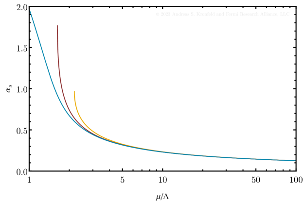
Figure 1: Gauge coupling $\alpha_{s}$ vs. $\mu/\Lambda$ in various schemes for $N_{c}=n_{f}=3$: $\alpha_{\overline{\rm MS}}(\mu)$ (gold), $\alpha_{\text{g}}(\mu)$ (red), and $\alpha_{2}(\mu)$ (blue). $\alpha_{\overline{\rm MS}}$ (with $1/\beta(\alpha)$ expanded to fixed order) and $\alpha_{\text{g}}$ run into branch points at $\mu\approx 2.1797\Lambda$ and $(\mathrm{e}/2b)^{b}\Lambda\approx 1.629\Lambda$, respectively. For smaller $\mu$, they are undefined. At these points, $\alpha_{\overline{\rm MS}}(2.1797\Lambda)=0.97601$, $\alpha_{\text{g}}(1.629\Lambda)=1.76715$. $\alpha_{2}(\mu)$ does not behave this way and like $\alpha_{\text{g}}$ has $\delta_{2}=0$.

Figure 1 shows the running of $\alpha_{\text{g}}$ and $\alpha_{2}$ ($\alpha_{n}$ for $n=2$), in SU(3) gauge theory with three massless flavors. The pole in the geometric $\beta$ function, which is the source of the problem, can be removed while retaining a closed-form relation between $\ln(\mu/\Lambda)$ and a family of schemes $\alpha_{n}$:

$$\beta(\alpha_{n}) =-\frac{\beta_{0}\alpha_{n}^{2}}{1-(\beta_{1}/\beta_{0})\alpha_{n}+n(\beta_{1}\alpha_{n}/\beta_{0})^{n+1}},$$ (39a)

$$\ln(\mu/\Lambda) =\frac{1}{2\beta_{0}\alpha_{n}}+b\ln(\beta_{0}\alpha_{n})-b\left(\frac{\beta_{1}\alpha_{n}}{\beta_{0}}\right)^{n}.$$ (39b)

In section 7, $\alpha_{2}$ is used to study how MRS works in practice. Like $\alpha_{\text{g}}$, $\alpha_{2}$ has $\delta_{2}=0$, so that $\mathbf{K}^{(p)}$ can be neglected (for $L\leq 4$). $\alpha_{\overline{\rm MS}}$ can be formulated by integrating the $\overline{\rm MS}$ $\beta$ function with either $1/\beta(\alpha_{\text{s}})$ or $\beta(\alpha_{\text{s}})$ expanded to fixed order. Both have an undesirable fixed point à la $\alpha_{\text{g}}$. Truncating with $\beta_{3}$, the former choice — also used in section 7 — is valid only for $\mu\geq 2.1797\Lambda$, at which point $\alpha_{\text{s}}=0.97601$ (cf., figure 1). The latter (again truncating with $\beta_{3}$) is valid only for $\mu\geq 0.87645\Lambda$, asymptotically as $\alpha_{\text{s}}\to\infty$ and in practice for $\alpha_{\text{s}}\gtrsim 50$.

6 Anomalous dimensions

The $Q$ dependence is not always as simple as the power law in eq. 1, because $C_{p}$ can depend on $Q$ via $\alpha_{\text{s}}(Q)$. In the operator-product expansion, for example, power corrections take the form

$$C_{p}(\mu/Q,\alpha_{\text{s}}(\mu))\frac{\langle\mathscr{O}(\mu)\rangle}{Q^{p}}=\widehat{C}_{p}(\alpha_{\text{s}}(Q))\frac{\langle\mathscr{O}_{\text{RGI}}\rangle}{Q^{p}}.$$ (40)

On the right-hand side, the renormalization group has been used to factor the $\mu$ dependence, such that $\langle\mathscr{O}_{\text{RGI}}\rangle\propto\Lambda^{p}$. The renormalization-group-invariant (RGI) Wilson coefficient can be written

$$\widehat{C}_{p}(\alpha_{\text{s}})=\left(2\beta_{0}\alpha_{\text{s}}\right)^{\psi}\sum_{l=-1}c_{l}\alpha_{\text{s}}^{l+1},$$ (41)

where $\psi=\gamma_{0}/2\beta_{0}$ and $\gamma_{0}$ is the one-loop anomalous dimension of $\mathscr{O}$. Some of the leading coefficients may (for some reason) vanish, and the series is known in practice only to some order. Strategies for truncating the series in eq. 41 lie beyond the scope of this paper.

Let us assume $c_{-1}\neq 0$. It is convenient to extend the matrix notation to $\boldsymbol{\mathfrak{A}}_{\text{g}}=\left\lceil 1\quad\alpha_{\text{g}}\quad\alpha_{\text{g}}^{2}\quad\alpha_{\text{g}}^{3}\quad\alpha_{\text{g}}^{4}\quad\cdots\;\right\rceil$, $\bm{r}_{\text{g}}=\left\lceil r_{-1}\quad r_{0}\quad r_{1}\quad r_{2}\quad r_{3}\quad\cdots\;\right\rceil^{\text{T}}$, and so on. The $r_{-1}$ entry is useful for bookkeeping; it cannot influence the final result, so below it can be set to 0, which is equivalent to changing to physical quantity to $\mathscr{R}(Q)-r_{-1}$.

To isolate $\Lambda^{p}$ so that it can be differentiated away, it is necessary to multiply by $Q^{p}/\widehat{C}_{p}$. Division by the Wilson coefficient changes the series $\boldsymbol{\mathfrak{A}}_{\text{g}}\cdot\bm{r}_{\text{g}}$ to $(2\beta_{0}\alpha_{\text{s}})^{-\psi}\boldsymbol{\mathfrak{A}}_{\text{g}}\cdot\mathbf{C}^{-1}\cdot\bm{r}_{\text{g}}$, where

$$\mathbf{C}=\left\lceil\begin{array}[]{ccccc}c_{-1}&0&0&0&\cdots\\ c_{0}&c_{-1}&0&0&\cdots\\ c_{1}&c_{0}&c_{-1}&0&\cdots\\ c_{2}&c_{1}&c_{0}&c_{-1}&\cdots\\ \vdots&\vdots&\ddots&\ddots&\ddots\end{array}\right\rceil.$$ (42)

The operation $\hat{Q}^{(p)}$ is applied to $(2\beta_{0}\alpha_{\text{s}})^{-\psi}\boldsymbol{\mathfrak{A}}_{\text{g}}\cdot\mathbf{C}^{-1}\bm{r}_{\text{g}}$, followed by multiplication by $\widehat{C}_{p}$. These steps yield $\boldsymbol{\mathfrak{A}}_{\text{s}}\cdot\bm{f}^{(p,\psi,\widehat{C})}_{\text{g}}$ with

$$\bm{f}^{(p,\psi,\widehat{C})}_{\text{g}}=\mathbf{C}\cdot\mathbf{Q}^{(p,\psi)}_{\text{g}}\cdot\mathbf{C}^{-1}\cdot\bm{r}_{\text{g}},$$ (43)

and $\mathbf{Q}^{(p,\psi)}_{\text{g}}$ has the same entries as in eq. 16 but with $l\to l-\psi$ and $k\to k-\psi$. The inverse ${\mathbf{Q}^{(p,\psi)}_{\text{g}}}^{-1}$ is given by eq. 17 with the same substitutions.

Equation 43 can be solved for

$$\bm{r}_{\text{g}}=\mathbf{C}\cdot{\mathbf{Q}^{(p,\psi)}_{\text{g}}}^{-1}\cdot\mathbf{C}^{-1}\cdot\bm{f}_{\text{g}}^{(p,\psi,\widehat{C})},$$ (44)

which has the same structure as the scheme change eq. 34. Thus,

$$\mathbf{C}\cdot{\mathbf{Q}^{(p,\psi)}_{\text{g}}}^{-1}\cdot\mathbf{C}^{-1}={\mathbf{Q}^{(p,\psi)}_{\text{g}}}^{-1}\cdot\left(\mathbf{1}+\mathbf{K}^{(p,\psi,\widehat{C})}\right),$$ (45)

and $\mathbf{K}^{(p,\psi,\widehat{C})}$ can be absorbed into the coefficients $\bm{f}_{\text{g}}^{(p,\psi,\widehat{C})}$, as in eq. 38 when estimating $r_{l}$, $l\geq L$. In the basic formulas for the improved series, eq. 19, it makes sense (along with $l\to l-\psi$ and $k\to k-\psi$) to change the conventional factor $\Gamma(1+pb)$ to $\Gamma(1+pb-\psi)$ and to omit $\psi$ in the powers of $2\beta_{0}/p$. The change to the normalization factor, $R_{0}^{(p,\psi)}$, is straightforward. In the Borel summation leading up to eq. 24, $\psi$ always appears as $pb-\psi$; the sum over $l$ and splitting of the integration follow exactly as in section 3.

If more than one power correction has an anomalous dimension, they still can be removed successively. Now every step affects all subsequent steps. The case of removing two power corrections reveals how complications ensue. Let the two power terms be $\widehat{C}_{i}\Lambda^{p_{i}}/Q^{p_{i}}$, $i=1,2$. The first step converts the second Wilson coefficient

$$\widehat{C}_{2} =(2\beta_{0}\alpha_{\text{s}})^{\psi_{2}}\boldsymbol{\mathfrak{A}}_{\text{s}}\cdot\bm{c}_{2}\mapsto\frac{p_{1}-p_{2}}{p_{1}}(2\beta_{0}\alpha_{\text{s}})^{\psi_{2}}\boldsymbol{\mathfrak{A}}_{\text{s}}\cdot\bm{c}_{2/1},$$ (46a)

$$\bm{c}_{2/1} =\mathbf{C}_{1}\cdot\mathbf{Q}^{(p_{1}-p_{2},\psi_{1}-\psi_{2})}\cdot\mathbf{C}_{1}^{-1}\cdot\bm{c}_{2}.$$ (46b)

The second step then leads to

$$\bm{f}^{\{(p_{1},\psi_{1},\widehat{C})_{1},(p_{2},\psi_{2},\widehat{C})_{2}\}}_{\text{g}}=\mathbf{C}_{2/1}\cdot\mathbf{Q}^{(p_{2},\psi_{2})}_{\text{g}}\cdot\mathbf{C}_{2/1}^{-1}\cdot\mathbf{C}_{1}\cdot\mathbf{Q}^{(p_{1},\psi_{1})}_{\text{g}}\cdot\mathbf{C}_{1}^{-1}\cdot\bm{r}_{\text{g}},$$ (47)

Note that the same outcome is obtained if the $\Lambda^{p_{2}}$ term is removed first, i.e.,

$$\mathbf{C}_{2/1}\cdot\mathbf{Q}^{(p_{2},\psi_{2})}_{\text{g}}\cdot\mathbf{C}_{2/1}^{-1}\cdot\mathbf{C}_{1}\cdot\mathbf{Q}^{(p_{1},\psi_{1})}_{\text{g}}\cdot\mathbf{C}_{1}^{-1}=\mathbf{C}_{1/2}\cdot\mathbf{Q}^{(p_{1},\psi_{1})}_{\text{g}}\cdot\mathbf{C}_{1/2}^{-1}\cdot\mathbf{C}_{2}\cdot\mathbf{Q}^{(p_{2},\psi_{2})}_{\text{g}}\cdot\mathbf{C}_{2}^{-1},$$ (48)

and similarly for their inverses. A decomposition of the right-hand side of eq. 47 along the lines of eq. 31 seems possible by isolating $\mathbf{Q}^{(p_{1},\psi_{1})}_{\text{g}}$ and $\mathbf{Q}^{(p_{2},\psi_{2})}_{\text{g}}$ and pragmatically absorbing the rest into the coefficients (as in eq. 45), but an elegant arrangement has (so far) eluded me.

Suppose the $c_{l}$ vanish for $l<n$. The first nonzero term, $c_{n}$, should not be connected to the $r_{l}$, $l\leq n$. A possible route forward is to subtract $\sum_{l=-1}^{n}r_{l}\alpha_{\text{s}}^{l+1}$ from $\mathscr{R}$, and the difference is still a valid observable. The factorially growing contributions can then be treated as before. If $p_{2}=p_{1}$ but $\psi_{2}\neq\psi_{1}$, the vector $\bm{c}_{2/1}$ in eq. 46 must be redefined as $-2\mathbf{C}_{1}\cdot\mathbf{D}^{(\psi_{1}-\psi_{2})}\cdot\mathbf{C}_{1}^{-1}\cdot\bm{c}_{2}$ with $c_{2/1,-1}=0$, so the second step will have to be tweaked in a similar way.

7 The static energy

To see MRS in action, the procedure is applied in this section to the gluonic energy stored between a static quark and a static antiquark, $E_{0}(r)$, called the “static energy” for short. It is computed in lattice gauge theory from the exponential fall-off at large $t$ of a $t\times r$ Wilson loop Wilson:1974sk ; Brambilla:2022het . The lattice quantity is the sum of a physical quantity plus twice the linearly divergent self-energy of a static quark. Dimensional regularization has no linear divergence, but on general grounds a constant of order $\Lambda$ is possible. Setting $\mathscr{R}(1/r)=-rE_{0}(r)/C_{F}$ yields a quantity of the form given in eq. 1 with $r_{-1}=0$ and $p=1$.

The static energy is a good candidate to test MRS because four orders in perturbation theory are known, thus enabling a thorough test. Beyond the tree-level result of order $\alpha_{\text{s}}$, $\overline{\rm MS}$-scheme results are available at order $\alpha_{\text{s}}^{2}$ Fischler:1977yf ; Billoire:1979ih , $\alpha_{\text{s}}^{3}$ Peter:1997me ; Schroder:1998vy ; Kniehl:2001ju , and $\alpha_{\text{s}}^{4}$ Smirnov:2008pn ; Anzai:2009tm ; Smirnov:2009fh ; Lee:2016cgz . The one-loop Gross:1973id ; Politzer:1973fx , two-loop Jones:1974mm ; Caswell:1974gg , three-loop Tarasov:1980au ; Larin:1993tp , and four-loop vanRitbergen:1997va ; Czakon:2004bu ; Zoller:2016sgq coefficients of the $\overline{\rm MS}$ $\beta$ function are also needed. The five-loop coefficient $\beta_{4}$ Baikov:2016tgj ; Herzog:2017ohr ; Luthe:2017ttc is not needed here.

References Fischler:1977yf ; Billoire:1979ih ; Peter:1997me ; Schroder:1998vy ; Kniehl:2001ju ; Smirnov:2008pn ; Anzai:2009tm ; Smirnov:2009fh ; Lee:2016cgz compute the static potential, $V(q)$, in momentum space, finding it to be infrared divergent starting at order $\alpha_{\text{s}}^{4}$ Appelquist:1977es . This behavior reflects the emergence of an “ultrasoft” scale $\alpha_{\text{s}}r^{-1}$ in addition to the hard scale $r^{-1}$. Ultrasoft contributions can be described in a multipole expansion and thereby demonstrated to render the static energy infrared finite Brambilla:1999qa ; Brambilla:1999xf ; Kniehl:1999ud . If $\alpha_{\text{s}}r^{-1}\gg\Lambda$, the ultrasoft part can be calculated perturbatively Brambilla:1999qa ; Kniehl:1999ud , and the total static energy is explicitly seen to be infrared finite Brambilla:1999qa ; Kniehl:1999ud ; Anzai:2009tm . A remnant of the cancellation remains in logarithms of the ratio of the two scales, $\ln[(\alpha_{\text{s}}r^{-1})/r^{-1}]=\ln\alpha_{\text{s}}$.

Following the exposition of Garcia i Tormo Tormo:2013tha , a momentum-space quantity, here denoted $\tilde{\mathscr{R}}(q)$, poses a second problem à la eq. 1, again with $r_{-1}=0$ but now with $p>1$. To distinguish the series coefficients associated with $\tilde{\mathscr{R}}(q)$ and $\mathscr{R}(1/r)$ from each other and the distance $r$, the notation used here is

$$\tilde{R}(q)=\sum_{l=0}a_{l}(\mu/q)\alpha_{\text{s}}(\mu)^{l+1},\quad\quad R(1/r)=\sum_{l=0}v_{l}(\mu r)\alpha_{\text{s}}(\mu)^{l+1}.$$ (49)

The coefficients $a_{l}(1)$ are available in the literature Fischler:1977yf ; Billoire:1979ih ; Peter:1997me ; Schroder:1998vy ; Kniehl:2001ju ; Smirnov:2008pn ; Anzai:2009tm ; Smirnov:2009fh ; Lee:2016cgz and can be found in a consistent notation in the accompanying Mathematica Mathematica:13.2.1 notebook. Each $v_{l}(\mu r)/r$ is $4\pi$ times the Fourier transform of $a_{l}(\mu/q)/q^{2}$. Indeed, the $p=1$ factorial growth of the $v_{l}$ arises from the Fourier transform of the logarithms (cf., eq. 4) in $a_{l}(\mu/q)$. The series $F^{(1)}(1/r)$, derived as in section 3 from $R(1/r)$, is related to the “static force”, $\mathfrak{F}(r)=-\mathrm{d}{E_{0}}/\mathrm{d}r$, by $\mathscr{F}(r)=F^{(1)}(1/r)=-r^{2}\mathfrak{F}(r)/C_{F}$. Note that $\mathfrak{F}(r)$ — and, hence $\mathscr{F}(r)$ and $F^{(1)}(1/r)$ — is expected to be free of renormalon ambiguities Brambilla:1999xf ; Ayala:2020odx , because the change in static energy from one distance to another is physical. The series $f_{l}$ should eventually exhibit factorial growth owing to instantons, i.e., with $p\geq 4\pi\beta_{0}={\textstyle\frac{11}{3}}C_{A}-{\textstyle\frac{4}{3}}\sum_{f}T_{f}$.

The remainder of this section gives numerical and graphical results for SU(3) gauge theory with three massless flavors. For brevity, the superscript “(1)” on $F^{(1)}$, $R_{0}^{(1)}$, etc., is omitted. To obtain numerical results and prepare plots, $\alpha_{\text{s}}$ in the ultrasoft logarithm, $\ln\alpha_{\text{s}}$, must be specified. This $\alpha_{\text{s}}$ can be taken to run, namely taken to be the same as the expansion parameter $\alpha_{\text{s}}(\mu)$. Alternatively, $\alpha_{\text{s}}$ can be held fixed. Below, $\alpha_{\text{s}}(s/r)$ (or $\alpha_{\text{s}}(sq)$), for various fixed $s$ is used as an expansion parameter, and the ultrasoft $\alpha_{\text{s}}$ is chosen either to be the same or, for comparison, a fixed value $\alpha_{\text{s}}={\textstyle\frac{1}{3}}$. This value arises at scales where perturbation theory starts to break down, making it a reasonable alternative. Resummation of logarithms $\alpha_{\text{s}}^{3+n}\ln^{n}\alpha_{\text{s}}$ Pineda:2000gza and $\alpha_{\text{s}}^{4+n}\ln^{n}\alpha_{\text{s}}$ Brambilla:2006wp ; Brambilla:2009bi is not considered here.

Table 3 shows the first four $a_{l}$ and $f_{l}$ in three different renormalization schemes, $\overline{\rm MS}$, geometric, and eq. 39 with $n=2$.

	$\overline{\rm MS}$		geometric		eq. 39, $n=2$
$l$	$a_{l}(1)$	$f_{l}(1)$	$a_{l}(1)$	$f_{l}(1)$	$a_{l}(1)$	$f_{l}(1)$
$0$	$1.0$	$1.0$	$1.0$	$1.0$	$1.0$	$1.0$
$1$	$0.557\,042$	$-0.048\,552$	$0.557\,042$	$-0.048\,552$	$0.557\,042$	$-0.048\,552$
$2$	$1.702\,18$	$0.687\,291$	$1.834\,97$	$0.820\,079$	$1.834\,97$	$0.820\,079$
$3$	$2.436\,87$	$0.323\,257$	$2.832\,68$	$0.558\,242$	$3.013\,89$	$0.739\,452$

Table 2: Perturbation series coefficients with $s=1$ for $\tilde{R}(q)$ ($a_{l}$) and $F(r)$ ($f_{l}$). Here $\alpha_{\text{s}}={\textstyle\frac{1}{3}}$ for $a_{3}$ and $f_{3}$.

	$\overline{\rm MS}$		geometric		eq. 39, $n=2$
$l$	$v_{l}(1)$	$v_{l}(1)-V_{l}(1)$	$v_{l}(1)$	$v_{l}(1)-V_{l}(1)$	$v_{l}(1)$	$v_{l}(1)-V_{l}(1)$
$0$	$1.0$	$0.206\,061$	$1.0$	$0.182\,531$	$1.0$	$0.177\,584$
$1$	$1.383\,84$	$-0.202\,668$	$1.383\,84$	$-0.249\,689$	$1.383\,84$	$-0.259\,574$
$2$	$5.462\,28$	$0.019\,479$	$5.595\,07$	$-0.009\,046$	$5.595\,07$	$-0.042\,959$
$3$	$26.6880$	$0.219\,262$	$27.3034$	$0.050\,179$	$27.4846$	$0.066\,468$

Table 3: Perturbation series coefficients with $s=1$ for $R(r)$ and $R_{\text{RS}}$ (with $V_{l}$ derived from $v_{l}$ as $R_{l}$ from $r_{l}$ in section 3). Here $\alpha_{\text{s}}={\textstyle\frac{1}{3}}$ for $v_{3}$ and $v_{l}-V_{l}$.

The scheme dependence in the two- and three-loop coefficients is about 10%. The (non)growth in $l$ conforms with expectations: $a_{l}$ is perhaps growing slowly and $f_{l}$ is not growing yet. (Recall, $p>1$ for $a_{l}$ and $p\geq 9$ for $f_{l}$.) Table 3 shows the first four $v_{l}$ in the same three schemes. The growth is obvious. Table 3 also shows the subtracted coefficients $v_{l}(1)-V_{l}(1)$. The cancellation is striking.

The cancellation at $s=1$ is robust, as shown in figure 2 over an illustrative interval of $\ln{s}$.

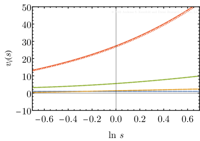
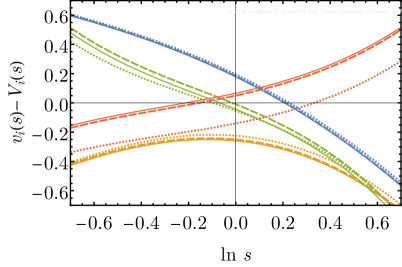
Figure 2: Scale dependence of $v_{l}(s)$ (left) and $v_{l}(s)-V_{l}(s)$ (right) vs. $\ln s$. Note the difference in vertical scale. Blue, gold, green, and red correspond to $l=0$, $1$, $2$, and $3$, respectively. Dotted, dashed, and solid curves correspond to the $\overline{\rm MS}$, geometric, and $\alpha_{2}$ schemes, respectively.

The range of $v_{3}(s)$ and even $v_{2}(s)$ dwarfs that of all $v_{l}(s)-V_{l}(s)$: $v_{3}(s)-V_{3}(s)$ ($v_{2}(s)-V_{2}(s)$) is 50–100 (5–10) times smaller than $v_{3}(s)$ ($v_{2}(s)$). Near $\ln s=0$, these two subtracted coefficients are unusually small. Overall, the cancellation is best for $\ln{s}\approx{\textstyle\frac{1}{4}}$, where $|v_{0}-V_{0}|$ is especially small, while the others are of typical size.

Interestingly, as $\ln s$ is taken negative both factors in the first term $[v_{l}(s)-V_{l}(s)]\alpha_{\text{s}}(s/r)$ increase. This behavior can be traced to the normalization factor $R_{0}(s)$, which is plotted in figure 3 for the three schemes.

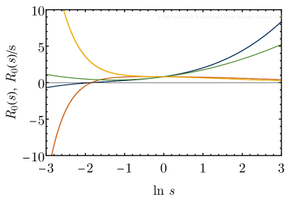
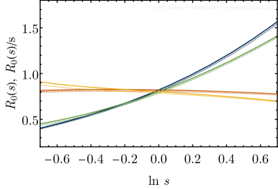
Figure 3: Scale dependence of $R_{0}(s)$ and $R_{0}(s)/s$ over a very wide range (left) and a relevant range (right). Blue and orange (green and yellow) curves corresponds to $L=4$ ($L=3$) in eq. 19b. Blue and green (orange and yellow) curves corresponds to $R_{0}(s)$ ($R_{0}(s)/s$). Dotted, dashed, and solid curves correspond to the $\overline{\rm MS}$, geometric, and $\alpha_{2}$ schemes, respectively.

There is not much scheme dependence. Curves for $L=4$ and $L=3$ in eq. 19b are shown. They are close, or even very close, to each other for $|\ln s|\leq\ln 2$. Sample numerical values are given in table 4, again using both four and three terms in eq. 19b. The shape of $R_{0}(s)$ follows from the positivity of the highest-power logarithmic term in eq. 4 and the positivity of the coefficients in eq. 19b. Near $\ln s=-2$, the four-term $R_{0}(s)$ goes negative, which is a reflection of $v_{3}(s)$ being run to an absurd extreme while omitting (unknown) higher orders. Indeed, the three-term approximation to $R_{0}(s)$ turns up near $\ln s=-2$, which is a reflection of $v_{2}(s)$ being run to an absurd extreme.

	$\overline{\rm MS}$		geometric		eq. 39, $n=2$
$s$	$L=4$	$L=3$	$L=4$	$L=3$	$L=4$	$L=3$
${\textstyle\frac{1}{2}}$	$0.386\,864$	$0.437\,281$	$0.403\,196$	$0.454\,397$	$0.397\,605$	$0.437\,281$
$1$	$0.793\,939$	$0.785\,114$	$0.817\,469$	$0.802\,230$	$0.801\,081$	$0.785\,114$
$2$	$1.523\,44$	$1.387\,07$	$1.554\,17$	$1.404\,19$	$1.526\,98$	$1.387\,07$

Table 4: Normalization factor $R_{0}(s)$ of the $p=$ factorial growth in three schemes for $s\in\{{\textstyle\frac{1}{2}},1,2\}$ at three ($L=4$) and two ($L=3$) loops. Here $\alpha_{\text{s}}={\textstyle\frac{1}{3}}$ for $L=4$.

Figure 3 also shows $R_{0}(s)/s$, which multiplies the term absorbed into the power correction (cf., last sentence in section 3). It is nearly constant over a wide range, especially once $L=4$.

The coefficients’ variation with $s$ is set up to compensate that of $\alpha_{\text{s}}(sq)$ or $\alpha_{\text{s}}(s/r)$. Figure 4 shows how $\tilde{R}(q)$, $F(1/r)$, $R(1/r)$, and $R_{\text{MRS}}(1/r)$ depend on $\Lambda/q$ or $r\Lambda$ for $s\in\{{\textstyle\frac{1}{2}},1,2\}$.

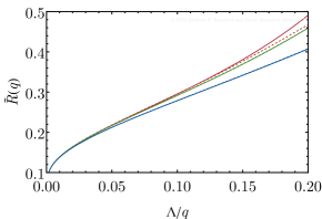
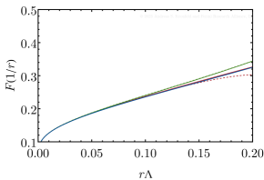
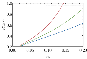
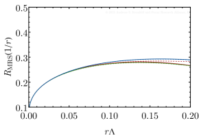
Figure 4: Scale variation in the $\alpha_{2}$ scheme up to and including the $\alpha_{\text{s}}^{4}$ term. Top: $\tilde{R}(q)$ and $F(1/r)$; neither suffers the $p=1$ renormalon. Bottom: $R(1/r)$ (with $p=1$ renormalon) and $R_{\text{MRS}}(1/r)$ (after MRS). Red, green, and blue curves correspond to $s={\textstyle\frac{1}{2}}$, $s=1$, and $s=2$, respectively. Solid (dashed) curves correspond to a running (fixed) $\alpha_{\text{s}}$ in the ultrasoft $\ln\alpha_{\text{s}}$. Note that the vertical scale for $R(1/r)$ is twice that of the other three plots.

(Plotted this way, the high-$q$, short-$r$ domain, where perturbation theory works best without any effort, is shrunk into a small region.) The variation with $s$ is mild for $\tilde{R}(q)$, even milder for $F(1/r)$, and catastrophic for $R(1/r)$. After MRS, however, the scale variation is as mild for $R_{\text{MRS}}(1/r)$ as for the renormalon-free $F(1/r)$. As shown in figure 5, the fractional difference of both remains a few percent for $r\Lambda\lesssim 0.1$ (with $s=1$ and running ultrasoft $\ln\alpha_{\text{s}}$ as the baseline).

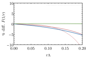
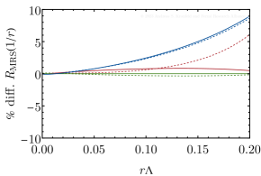
Figure 5: Scale variation in the $\alpha_{2}$ scheme of the fractional difference of $F(1/r)$ (left) and $R_{\text{MRS}}(1/r)$ (right), with respect to $s=1$ with running ultrasoft $\alpha_{\text{s}}$. Curve and color code as in figure 4.

The mild variation with $s$ is a pleasant outcome given the $s$ dependence of the subtracted coefficients (cf., figure 2). Figure 6 shows the variation with $s$ as a function of $r$ of the Borel sum $R_{\text{B}}(1/r)$ (left, eq. 26) and the subtracted series $R_{\text{RS}}(1/r)$ for $L=4$ (right).

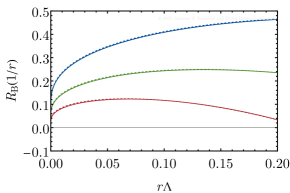
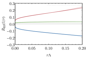
Figure 6: Scale variation in the $\alpha_{2}$ scheme of the Borel sum $R_{\text{B}}(1/r)$ (left) and the $L=4$-subtracted series $R_{\text{RS}}(1/r)$ (right). Curve and color code as in figure 4.

Both are quite sensitive to $s$, but their sum (bottom right of figure 4) is not.

The first two orders suffice to lift the $s$ dependence, as shown in section 7. Here, $R_{\text{B}}(1/r)$ is shown (dotted curve) and each term $(v_{l}-V_{l})\alpha_{\text{s}}^{l+1}$, $l=0,1,2,3$, in $R_{\text{RS}}(1/r)$ is accumulated (dashed curves with longer dashes as the order increases) until the total $L=4$ (solid) result $R_{\text{MRS}}(1/r)$ is reached.

Borel sum $R_{\text{B}}(1/r)$ (dotted curves) accumulating successively each term $(v_{l}-V_{l})\alpha_{\text{s}}^{l+1}$ (dashed curves with longer dashes for larger $l$) in the three schemes. Solid curves for the full $R_{\text{MRS}}$. Color code as in figure 4.[0.49] Same as figure 4 (bottom right) but with a band stemming from the uncertainty in $R_{0}$ (taken equal to the last term in eq. 19b) and an expanded vertical scale. Curve and color code as in figure 4.[0.49]

Adding the tree-level term $(v_{0}-V_{0})\alpha_{\text{s}}$ to the Borel sum overshoots the full (solid) result, but adding the one-loop term $(v_{1}-V_{1})\alpha_{\text{s}}^{2}$ yields a curve almost indistinguishable from $R_{\text{MRS}}(1/r)$. Indeed, it is hard to distinguish the longer-dashed curves from the solid ones, underscoring that the two-loop term $(v_{2}-V_{2})\alpha_{\text{s}}^{3}$ makes a small change while the three-loop term $(v_{3}-V_{3})\alpha_{\text{s}}^{4}$ makes hardly any change. As with the pole mass Brambilla:2017hcq , MRS perturbation theory converges (in the practical sense) quickly.

Let us return to the term-by-term change in $R_{0}$ (cf., figure 3 and table 4). The highest-order term in eq. 19b can be used to estimate the uncertainty in $R_{0}$ from omitting even higher orders Brambilla:2017hcq . In the case at hand, the term with $f_{3}$ yields the estimate, which is around $10\%$ or less (cf., table 4). Section 7 (right) overlays the resulting $s=1$ uncertainty band on $R_{\text{MRS}}(1/r)$ on the curves (at various $s$) of figure 4 (bottom right). The uncertainty propagated to $R_{\text{MRS}}$ is smaller than $10\%$ because changes in $R_{0}$ push $R_{\text{B}}(1/r)$ and $R_{\text{RS}}(1/r)$ in opposite directions. Indeed, the uncertainty in $R_{\text{MRS}}$ stemming from $R_{0}$ is smaller than the difference between the $s=1$ and the $s={\textstyle\frac{1}{2}}$ and 2 curves. Note, however, that the $R_{0}$-uncertainty, as defined here, is smaller at $s=1$ than at $s={\textstyle\frac{1}{2}}$ and 2 (cf., figure 3 and table 4). The uncertainty bands of these other choices (not shown) cover all three.

8 Summary and outlook

The initial aim of this work was to study and extend the discussion of factorial growth and renormalons started in refs. Komijani:2017vep ; Brambilla:2017hcq . I found, however, that the perspective, derivation, and interpretation could be simplified: a straightforward analysis extracts information from the renormalization-group constraints on the series coefficients. The only other ingredient is the knowledge (or assumption) of the powers $\{p_{i}\}$ of the power-suppressed corrections to the perturbative series of a physical observable. A by-product of adding this information to the series is to subtract the leading factorial growth (aka “renormalon effects”) from the first few series coefficients. Remarkably, the factorial growth is not just a large-order phenomenon: it starts at low orders. How it comes to dominate the coefficients depends of the power of the power correction. (The lower the power, the more powerful the factorial!)

The worked example of the static energy (section 7) seems successful in removing a power correction of order $r\Lambda$ from (a dimensionless version of the) static energy, $-rE_{0}/C_{F}$. The conventional choice of $\mu=1/r$ (in the $\overline{\rm MS}$ scheme) seems near an optimum: perturbation theory converges with the MRS treatment as well as it does for the static force, which is thought to suffer corrections only of high power. Varying $\mu$ by a factor of two rearranges contributions between the tree and one-loop fixed order contributions, on the one hand, and (a specific definition of) the Borel sum of the factorial growth, on the other. At very short distances, $r\Lambda\lesssim{\textstyle\frac{1}{16}}$, the total result (using all information through order $\alpha_{\text{s}}^{4}$) does not vary over a wide range of $\mu$. It will therefore be interesting to fit to lattice-QCD data (e.g., that of ref. Brambilla:2022het ) and compare with other approaches to taming the series. (Some other approaches are described in refs. Takaura:2018vcy ; Bazavov:2019qoo ; Ayala:2020odx ; Ananthanarayan:2020umo ; Brambilla:2021wqs ; Sumino:2020mxk and earlier work cited there.)

Some practical issues remain before applying the MRS procedure to, say, an $\alpha_{\text{s}}$ determinations. The MRS method, like standard perturbation theory, does not say what scale $s$ to choose: starting in the $\overline{\rm MS}$ scheme with $s=1$ and varying by a factor of 2 is conventional. When the factorial growth of coefficients matters, i.e., when MRS has something to offer, the $\ln^{n}s$ contributions associated with scale setting cannot tame the coefficients. Scale setting in light of MRS may warrant a closer look. Another issue is that in many applications, some of the quarks cannot be taken massless. A nonzero quark mass in a loop alters the loop’s growth, removing the factorials from the infrared. It is probably best to add massive quark-loop effects at fixed order and not to use the massless result as a stand-in for the massive one Hoang:2000fm . Last, when anomalous dimensions are an important feature for more than one round of MRS, the method (as presented in section 6) remains to cumbersome to be appealing. It may suffice to neglect the anomalous dimensions, but only practical experience will tell.

Appendix A Modified Borel summation

Alternatives to the standard Borel resummation are possible Brown:1992pk , and a natural variant is pursued here, leading to the same endpoint. Start with eq. 21:

$$R_{\text{B}}^{(p)}\equiv\sum_{l=0}^{\infty}R_{l}^{(p)}\alpha^{l+1}=R_{0}^{(p)}\alpha\sum_{l=0}^{\infty}\left(\frac{2\beta_{0}\alpha}{p}\right)^{l}\frac{\Gamma(l+1+pb)}{\Gamma(1+pb)}.$$ (50)

The $l$-dependent $\Gamma$ function can be expressed as $\Gamma(l+1+pb)=\int_{0}^{\infty}t^{l+pb}\mathrm{e}^{-t}\mathrm{d}{t}$. Swapping the order of summation and integration

$$R_{\text{B}}^{(p)}=\frac{R_{0}^{(p)}\alpha}{\Gamma(1+pb)}\int_{0}^{\infty}\sum_{l=0}^{\infty}\left(\frac{2\beta_{0}\alpha t}{p}\right)^{l}t^{pb}\mathrm{e}^{-t}\mathrm{d}{t}=\frac{R_{0}^{(p)}\alpha}{\Gamma(1+pb)}\int_{0}^{\infty}\frac{t^{pb}\mathrm{e}^{-t}}{1-2\beta_{0}\alpha t/p}\mathrm{d}{t},$$ (51)

which only has a simple pole instead of a branch point. After integrating

$$R_{\text{B}}^{(p)}=R_{0}^{(p)}\frac{p}{2\beta_{0}}\mathscr{J}(pb,p/2\beta_{0}\alpha)-R_{0}^{(p)}\mathrm{e}^{\pm\mathrm{i}pb\pi}\frac{p^{1+pb}}{2^{1+pb}\beta_{0}}\Gamma(-pb)\left[\frac{\mathrm{e}^{-1/2\beta_{0}\alpha}}{(\beta_{0}\alpha)^{b}}\right]^{p},$$ (52)

where the factor $\mathrm{e}^{\pm\mathrm{i}pb\pi}$ in the second term corresponds to passing the contour below or above the pole. As before, the second term can be absorbed into the power correction, and the first — the principal part — is taken to define $R_{\text{B}}^{(p)}$, the same as eq. 24.

- (1) Fermilab Lattice, MILC, TUMQCD collaboration, Up-, down-, strange-, charm-, and bottom-quark masses from four-flavor lattice QCD, Phys. Rev. D 98 (2018) 054517 [1802.04248].
- (2) TUMQCD collaboration, Relations between heavy-light meson and quark masses, Phys. Rev. D 97 (2018) 034503 [1712.04983].
- (3) J. Komijani, A discussion on leading renormalon in the pole mass, J. High Energy Phys. 2017 (2017) 62 [1701.00347].
- (4) C.M. Bender and T.T. Wu, Large-order behavior of perturbation theory, Phys. Rev. Lett. 27 (1971) 461.
- (5) C.M. Bender and T.T. Wu, Anharmonic oscillator II: A study of perturbation theory in large order, Phys. Rev. D 7 (1973) 1620.
- (6) D.J. Gross and A. Neveu, Dynamical symmetry breaking in asymptotically free field theories, Phys. Rev. D 10 (1974) 3235.
- (7) B.E. Lautrup, On high order estimates in QED, Phys. Lett. B 69 (1977) 109.
- (8) G. ’t Hooft, Can we make sense out of quantum chromodynamics?, in The Whys of Subnuclear Physics, A. Zichichi, ed., (New York), pp. 943–982, Plenum, 1979.
- (9) M. Beneke, Renormalons, Phys. Rept. 317 (1999) 1 [hep-ph/9807443].
- (10) T. Lee, Renormalons beyond one loop, Phys. Rev. D 56 (1997) 1091 [hep-th/9611010].
- (11) T. Lee, Normalization constants of large order behavior, Phys. Lett. B 462 (1999) 1 [hep-ph/9908225].
- (12) A. Pineda, Determination of the bottom quark mass from the (1S) system, J. High Energy Phys. 06 (2001) 022 [hep-ph/0105008].
- (13) A.H. Hoang, A. Jain, I. Scimemi and I.W. Stewart, Infrared renormalization-group flow for heavy-quark masses, Phys. Rev. Lett. 101 (2008) 151602 [0803.4214].
- (14) L.S. Brown, L.G. Yaffe and C.-X. Zhai, Large-order perturbation theory for the electromagnetic current-current correlation function, Phys. Rev. D 46 (1992) 4712 [hep-ph/9205213].
- (15) A.F. Falk and M. Neubert, Second-order power corrections in the heavy-quark effective theory I: Formalism and meson form factors, Phys. Rev. D 47 (1993) 2965 [hep-ph/9209268].
- (16) A.F. Falk, M. Neubert and M.E. Luke, Residual mass term in the heavy quark effective theory, Nucl. Phys. B 388 (1992) 363 [hep-ph/9204229].
- (17) T. Mannel, Higher order corrections at zero recoil, Phys. Rev. D 50 (1994) 428 [hep-ph/9403249].
- (18) A.S. Kronfeld, Perturbative pole mass in QCD, Phys. Rev. D 58 (1998) 051501 [hep-ph/9805215].
- (19) I.I.Y. Bigi and N.G. Uraltsev, Anathematizing the Guralnik-Manohar bound for , Phys. Lett. B 321 (1994) 412 [hep-ph/9311337].
- (20) I.I.Y. Bigi, M.A. Shifman, N.G. Uraltsev and A.I. Vainshtein, Pole mass of the heavy quark: Perturbation theory and beyond, Phys. Rev. D 50 (1994) 2234 [hep-ph/9402360].
- (21) M. Beneke and V.M. Braun, Heavy quark effective theory beyond perturbation theory: Renormalons, the pole mass and the residual mass term, Nucl. Phys. B 426 (1994) 301 [hep-ph/9402364].
- (22) M. Beneke, More on ambiguities in the pole mass, Phys. Lett. B 344 (1995) 341 [hep-ph/9408380].
- (23) M.E. Luke, A.V. Manohar and M.J. Savage, Renormalons in effective field theories, Phys. Rev. D 51 (1995) 4924 [hep-ph/9407407].
- (24) M. Abramowitz and I.A. Stegun, Handbook of Mathematical Functions, Dover, New York (1972).
- (25) C. Ayala, G. Cvetič and A. Pineda, The bottom quark mass from the (1S) system at NNNLO, J. High Energy Phys. 09 (2014) 045 [1407.2128].
- (26) R.M. Corless, G.H. Gonnet, D.E.G. Hare, D.J. Jeffrey and D.E. Knuth, On the Lambert function, Adv Comp. Math. 5 (1996) 329.
- (27) K.G. Wilson, Confinement of quarks, Phys. Rev. D 10 (1974) 2445.
- (28) TUMQCD collaboration, Static energy in ()-flavor lattice QCD: Scale setting and charm effects, Phys. Rev. D 107 (2023) 074503 [2206.03156].
- (29) W. Fischler, Quark-antiquark potential in QCD, Nucl. Phys. B 129 (1977) 157.
- (30) A. Billoire, How heavy must quarks be in order to build Coulombic bound states?, Phys. Lett. B 92 (1980) 343.
- (31) M. Peter, The static potential in QCD: A full two loop calculation, Nucl. Phys. B 501 (1997) 471 [hep-ph/9702245].
- (32) Y. Schröder, The static potential in QCD to two loops, Phys. Lett. B 447 (1999) 321 [hep-ph/9812205].
- (33) B.A. Kniehl, A.A. Penin, M. Steinhauser and V.A. Smirnov, Non-Abelian heavy-quark–antiquark potential, Phys. Rev. D 65 (2002) 091503 [hep-ph/0106135].
- (34) A.V. Smirnov, V.A. Smirnov and M. Steinhauser, Fermionic contributions to the three-loop static potential, Phys. Lett. B 668 (2008) 293 [0809.1927].
- (35) C. Anzai, Y. Kiyo and Y. Sumino, Static QCD potential at three-loop order, Phys. Rev. Lett. 104 (2010) 112003 [0911.4335].
- (36) A.V. Smirnov, V.A. Smirnov and M. Steinhauser, Three-loop static potential, Phys. Rev. Lett. 104 (2010) 112002 [0911.4742].
- (37) R.N. Lee, A.V. Smirnov, V.A. Smirnov and M. Steinhauser, Analytic three-loop static potential, Phys. Rev. D 94 (2016) 054029 [1608.02603].
- (38) D.J. Gross and F. Wilczek, Ultraviolet behavior of non-Abelian gauge theories, Phys. Rev. Lett. 30 (1973) 1343.
- (39) H.D. Politzer, Reliable perturbative results for strong interactions?, Phys. Rev. Lett. 30 (1973) 1346.
- (40) D.R.T. Jones, Two-loop diagrams in Yang-Mills theory, Nucl. Phys. B 75 (1974) 531.
- (41) W.E. Caswell, Asymptotic behavior of non-Abelian gauge theories to two-loop order, Phys. Rev. Lett. 33 (1974) 244.
- (42) O.V. Tarasov, A.A. Vladimirov and A.Y. Zharkov, The Gell-Mann–Low function of QCD in the three-loop approximation, Phys. Lett. B 93 (1980) 429.
- (43) S.A. Larin and J.A.M. Vermaseren, The three-loop QCD -function and anomalous dimensions, Phys. Lett. B 303 (1993) 334 [hep-ph/9302208].
- (44) T. Van Ritbergen, J.A.M. Vermaseren and S.A. Larin, The four-loop -function in quantum chromodynamics, Phys. Lett. B 400 (1997) 379 [hep-ph/9701390].
- (45) M. Czakon, The four-loop QCD -function and anomalous dimensions, Nucl. Phys. B 710 (2005) 485 [hep-ph/0411261].
- (46) M.F. Zoller, Four-loop QCD -function with different fermion representations of the gauge group, J. High Energy Phys. 2016 (2016) 118 [1608.08982].
- (47) P.A. Baikov, K.G. Chetyrkin and J.H. Kühn, Five-loop running of the QCD coupling constant, Phys. Rev. Lett. 118 (2017) 082002 [1606.08659].
- (48) F. Herzog, B. Ruijl, T. Ueda, J.A.M. Vermaseren and A. Vogt, The five-loop beta function of Yang-Mills theory with fermions, J. High Energy Phys. 2017 (2017) 090 [1701.01404].
- (49) T. Luthe, A. Maier, P. Marquard and Y. Schröder, Complete renormalization of QCD at five loops, J. High Energy Phys. 2017 (2017) 020 [1701.07068].
- (50) T. Appelquist, M. Dine and I.J. Muzinich, Static limit of quantum chromodynamics, Phys. Rev. D 17 (1978) 2074.
- (51) N. Brambilla, A. Pineda, J. Soto and A. Vairo, Infrared behavior of the static potential in perturbative QCD, Phys. Rev. D 60 (1999) 091502 [hep-ph/9903355].
- (52) N. Brambilla, A. Pineda, J. Soto and A. Vairo, Potential NRQCD: An effective theory for heavy quarkonium, Nucl. Phys. B 566 (2000) 275 [hep-ph/9907240].
- (53) B.A. Kniehl and A.A. Penin, Ultrasoft effects in heavy quarkonium physics, Nucl. Phys. B 563 (1999) 200 [hep-ph/9907489].
- (54) X. Garcia i Tormo, Review on the determination of from the QCD static energy, Mod. Phys. Lett. A 28 (2013) 1330028 [1307.2238].
- (55) Wolfram Research, Inc., Mathematica, Version 13.2.1, Champaign, Illinois (2022).
- (56) C. Ayala, X. Lobregat and A. Pineda, Determination of from a hyperasymptotic approximation to the energy of a static quark-antiquark pair, J. High Energy Phys. 09 (2020) 016 [2005.12301].
- (57) A. Pineda and J. Soto, The renormalization group improvement of the QCD static potentials, Phys. Lett. B 495 (2000) 323 [hep-ph/0007197].
- (58) N. Brambilla, X. Garcia i Tormo, J. Soto and A. Vairo, The logarithmic contribution to the QCD static energy at N4LO, Phys. Lett. B 647 (2007) 185 [hep-ph/0610143].
- (59) N. Brambilla, A. Vairo, X. Garcia i Tormo and J. Soto, QCD static energy at next-to-next-to-next-to leading-logarithmic accuracy, Phys. Rev. D 80 (2009) 034016 [0906.1390].
- (60) H. Takaura, T. Kaneko, Y. Kiyo and Y. Sumino, Determination of from static QCD potential: OPE with renormalon subtraction and lattice QCD, J. High Energy Phys. 04 (2019) 155 [1808.01643].
- (61) TUMQCD collaboration, Determination of the QCD coupling from the static energy and the free energy, Phys. Rev. D 100 (2019) 114511 [1907.11747].
- (62) B. Ananthanarayan, D. Das and M.S.A. Alam Khan, QCD static energy using optimal renormalization and asymptotic Padé-approximant methods, Phys. Rev. D 102 (2020) 076008 [2007.10775].
- (63) N. Brambilla, V. Leino, O. Philipsen, C. Reisinger, A. Vairo and M. Wagner, Lattice gauge theory computation of the static force, Phys. Rev. D 105 (2022) 054514 [2106.01794].
- (64) Y. Sumino and H. Takaura, On renormalons of static QCD potential at and , J. High Energy Phys. 05 (2020) 116 [2001.00770].
- (65) A.H. Hoang, Bottom quark mass from mesons: Charm mass effects, hep-ph/0008102.