Novel-View Acoustic Synthesis from 3D Reconstructed Rooms

Abstract

We investigate the benefit of combining blind audio recordings with 3D scene information for novel-view acoustic synthesis. Given audio recordings from 2–4 microphones and the 3D geometry and material of a scene containing multiple unknown sound sources, we estimate the sound anywhere in the scene. We identify the main challenges of novel-view acoustic synthesis as sound source localization, separation, and dereverberation. While naively training an end-to-end network fails to produce high-quality results, we show that incorporating room impulse responses (RIRs) derived from 3D reconstructed rooms enables the same network to jointly tackle these tasks. Our method outperforms existing methods designed for the individual tasks, demonstrating its effectiveness at utilizing 3D visual information. In a simulated study on the Matterport3D-NVAS dataset, our model achieves near-perfect accuracy on source localization, a PSNR of $26.44\text{\,}\mathrm{dB}$ and a SDR of $14.23\text{\,}\mathrm{dB}$ for source separation and dereverberation, resulting in a PSNR of $25.55\text{\,}\mathrm{dB}$ and a SDR of $14.20\text{\,}\mathrm{dB}$ on novel-view acoustic synthesis. Code, pretrained models, and video results are available on the project webpage [1].

Index Terms—  novel-view acoustic synthesis, source localization, source separation, dereverberation

1 Introduction

Recent advancements in novel-view synthesis and 3D reconstruction [2, 3, 4] have enabled users to explore scenes freely, viewing them from positions not captured during recordings. However, a significant limitation of these approaches is the absence of sound, restricting the immersive experience. In contrast to novel-view image synthesis, the non-stationary nature of sound and the low resolution of microphones make novel-view acoustic synthesis a challenging problem [5].

In this work, we investigate novel-view acoustic synthesis in 3D reconstructed and calibrated rooms. We build upon recent developments in 3D reconstruction [2] and acoustic calibration techniques [6, 7, 8] and assume the availability of high-quality room geometry and acoustic material information. We also assume to have audio recordings from a limited microphone array (2–4 receivers) at known locations in the scene. However, we have no knowledge about the sound sources, including their number, locations, and content. Under this setting, our goal is to enable users moving freely in the scene to hear realistic spatial audio renderings of the unknown sound sources recorded by the microphones.

Novel-view acoustic synthesis remains challenging despite having 3D reconstructed rooms. The main problem is the lack of knowledge of the sound sources. With known sound sources, the audio at any new location can be produced using standard acoustic renderers [9, 10, 11, 12]. In other words, the key to novel-view acoustic synthesis is estimating the positions (i.e., sound localization) and the content (i.e., sound separation and dereverberation) of the sources from blind audio recordings. However, the limited number and resolution of microphones and the mixture of different reverberant sound in same audios makes these problems difficult, particularly if the semantics are similar (i.e., two people speaking) or the sounds arrive from close directions. Existing methods relying on time-delay cues cannot pinpoint the locations of multiple sound sources in a complex 3D scene [13]. Simply training a neural network also fails to generate high-quality results, as will be shown in Section 4.

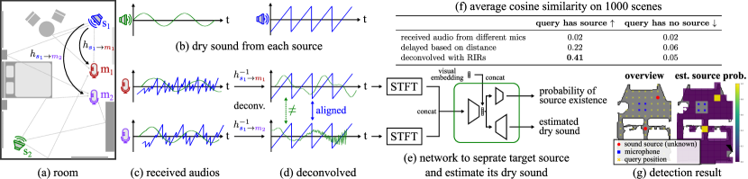
Fig. 1: Model overview and motivation. Given a 3D reconstructed room (a) and audio recordings from microphones (c), we estimate the locations and dry sound of individual sound sources. (d,f) Our key observation is that deconvolving audio recordings with the impulse response from a specific source location aligns sound emitted at that location across input recordings while keeping sound from other locations uncorrelated. (e) We use a network to isolate target audio from the mixture of sounds and mitigate deconvolution artifacts. (g) Our source detection result on an example scene. Our network accurately identify where the sound sources are.

Our key observation is that the echoes caused by the multipath reflection of sound contain valuable information for acoustic scene reconstruction. Specifically, as shown in Fig. 1, we propose to assist the network by deconvolving audio recordings from individual microphones (c) with RIRs from a specific location. This operation aligns the sound emitted from that location across microphone channels while keeping sound from other locations uncorrelated (d), enabling the network to predict whether an audio source exists at that location and the corresponding dry sound. Iterating this approach over all candidate source locations enables us to reconstruct the acoustic scene with high spatial resolution (g) and render it from novel viewpoints. Additionally, if we incorporate semantic visual cues (i.e., RGB images), we can further enhance source localization. We thoroughly study the benefits of deconvolution, as well as the use of visual cues, in experiments on the Matterport3D-NVAS dataset.

Contributions

Our method advances novel-view acoustic synthesis by leveraging RIRs for source localization, separation, and dereverberation. Our technique can reconstruct acoustic scenes with semantically indistinguishable sources, such as two guitars in the same room. To our knowledge, ours is the first method for novel-view acoustic synthesis to work for multiple sound sources. Additionally, our model can generalize to new scenes without per-scene optimization, as scene-specific information is encoded in the deconvolved audios, making our model scene-agnostic.

2 Related Work

Our approach relies on RIR estimation techniques that operate on 3D reconstructed rooms [6, 7, 8, 14, 15, 16]. These techniques estimate or render RIRs by using both room geometry and estimated acoustic material properties.

There are extensive studies separately addressing the tasks of sound localization [17], separation [18, 19, 20, 21, 22, 23], and dereverberation [24]. These generally do not take 3D scene information into account, which is useful for novel-view acoustic synthesis. Although the active audio-visual separation method [25] provides separation with 3D localization, it requires 3D embodied agents moving within the space.

Conceptually, our method is related to beamforming techniques [26, 27, 13, 28, 29, 30, 31], where the objective is to isolate the source at a query location, typically in non-reverberant scenarios (e.g., open spaces), relying on the directionality of sound. In contrast, our method utilizes 3D scene geometry and performs dereverberation simultaneously.

Recently, Chen et al. [5] introduced ViGAS, a pioneering end-to-end approach for novel-view acoustic synthesis, using images to synthesize binaural audio. While their method offers valuable insights, it does not address sound separation and is demonstrated only for a single source. It also does not utilize 3D scene geometry. In contrast, our method leverages 3D scene geometry for sound localization and separation, enabling it to handle multiple sources.

3 Method

Our method decomposes the novel-view acoustic synthesis into two subproblems: (i) acoustic scene reconstruction, which involves 3D source localization, separation, and dereverberation, and (ii) novel-view acoustic rendering. We begin by introducing each problem and then present our approach.

3.1 Problem formulation

Acoustic scene reconstruction

Given recorded audio $y_{m}(t)$ from $M$ microphones and a 3D reconstructed room containing $S$ sound sources, we estimate the dry sound emitted by each source $\{x_{s}\}_{s=1}^{S}$, and their locations ${\mathcal{P}}\,{=}\,\{{\mathbf{p}}_{s}\}_{s=1}^{S}$. The recorded audio from microphone located at $\{{\mathbf{r}}_{m}\}_{m=1}^{M}$ is

$$y_{m}(t)=\sum_{s=1}^{S}{h_{{\mathbf{p}}_{s}\rightarrow{\mathbf{r}}_{m}}}(t)\ast x_{s}(t)+\psi_{m}(t),$$ (1)

where ${h_{{\mathbf{p}}_{s}\rightarrow{\mathbf{r}}_{m}}}$ denotes the RIR from ${\mathbf{p}}_{s}$ to ${\mathbf{r}}_{m}$, and $\psi_{m}(t)$ is the noise. Here we assume the RIRs are given from a 3D room reconstruction [6, 14, 7, 8, 15, 16]. We discuss robustness to the RIR estimation in the supplementary material [1].

Novel-view acoustic rendering

Once the acoustic scene is known, novel-view acoustic rendering is straightforward as it can be achieved by simply convolving the dry sound results with corresponding RIRs for novel viewpoints. The audio $y(t)$ from novel microphone located at ${\mathbf{r}}$ is given by:

$$y(t)=\sum_{s=1}^{S}h_{{\mathbf{p}}_{s}\rightarrow{\mathbf{r}}}(t)\ast x_{s}(t).$$ (2)

3.2 Our approach

Overview

We reconstruct the acoustic scene by querying potential 3D source locations within a room. Our goal is to determine: (i) the existence of a source at a query location and (ii) if present, its associated dry sound. By iterating this process across potential source locations, we effectively localize, separate, and dereverberate all sources in the room.

Specifically, for a set of candidate source locations, denoted as ${\mathcal{Q}}\,{=}\,\{{\mathbf{q}}_{n}\}_{n=1}^{N}$, which includes the actual source locations ${\mathcal{P}}$ (i.e., ${\mathcal{P}}\subset{\mathcal{Q}}$), the network provides two outputs: (i) a detection estimate ${\hat{d}}$, indicating the presence of a source, $\mathbf{1}_{\mathcal{P}}({\mathbf{q}}_{n})$, and (ii) an estimation ${\hat{x}}_{n}(t)$ of the isolated dry sound $x_{s}(t)$ at the query point ${\mathbf{q}}_{n}$ when a positive detection is made. Then, novel-view acoustic synthesis is achieved by

$$y(t)=\sum_{n=1}^{N}h_{{\mathbf{q}}_{n}\rightarrow{\mathbf{r}}}(t)\ast\left({\hat{x}}_{n}(t)\ \mathbf{1}({\hat{d}}>0.5)\right).\vspace{-2mm}$$ (3)

Deconvolution and cleaning

One challenge for processing multichannel audios from microphones at different locations is that the audios do not align across the channels. The delay and echo received by individual channel depend on source and microphone locations (e.g., see Fig. 1c) and can change dramatically across scenes. Thus, a U-Net [32], which performs well on single-channel source separation, fails with multiple channels when applied directly (see Section 4).

Our key observation is that after deconvolving individual recorded audios with the RIR from a specific 3D location to a microphone, the sound emitted from the location (if any) would align across microphones. Specifically, given a query point ${\mathbf{q}}_{n}$ and microphone $m$, we deconvolve the recorded audio $y_{m}(t)$ with the RIR ${h_{{\mathbf{q}}_{n}\rightarrow{\mathbf{r}}_{m}}}(t)$. In the frequency domain, the deconvolved audio can be represented as

$$Z_{nm}(w)=\sum_{s=1}^{S}\frac{{H_{{\mathbf{p}}_{s}\rightarrow{\mathbf{r}}_{m}}}(w)}{{H_{{\mathbf{q}}_{n}\rightarrow{\mathbf{r}}_{m}}}(w)}\ X_{s}(w)+\frac{\Psi_{m}(w)}{{H_{{\mathbf{q}}_{n}\rightarrow{\mathbf{r}}_{m}}}(w)},\vspace{-1mm}$$ (4)

where $X_{s}$, ${H_{{\mathbf{p}}_{s}\rightarrow{\mathbf{r}}_{m}}}$, ${H_{{\mathbf{q}}_{n}\rightarrow{\mathbf{r}}_{m}}}$, and $\Psi_{m}$ represent the Fourier transform of $x_{s}$, ${h_{{\mathbf{p}}_{s}\rightarrow{\mathbf{r}}_{m}}}$, ${h_{{\mathbf{q}}_{n}\rightarrow{\mathbf{r}}_{m}}}$, and $\psi_{m}$, respectively.

When ${\mathbf{q}}_{n}$ corresponds to source $i$ (i.e., ${\mathbf{q}}_{n}={\mathbf{p}}_{i}$), we have $Z_{nm}(w)=X_{i}(w)+\sum_{s\neq i}\frac{{H_{{\mathbf{p}}_{s}\rightarrow{\mathbf{r}}_{m}}}(w)}{{H_{{\mathbf{q}}_{n}\rightarrow{\mathbf{r}}_{m}}}(w)}X_{s}(w)+\frac{\Psi_{m}(w)}{{H_{{\mathbf{q}}_{n}\rightarrow{\mathbf{r}}_{m}}}(w)}$, or $Z_{nm}(w)=X_{i}(w)$ + noise. Notice that $X_{i}$ is independent to $m$, which means that the deconvolved audios for individual microphones, $\{Z_{nm}\}_{m=1}^{M}$, consistently contain $X_{i}(w)$, the dry sound emitted by source $i$. Sound from other sources are unaligned and become noise-like. When ${\mathbf{q}}_{n}$ contains no sound source, no such alignment would exist. Fig. 1f shows the average cosine similarity between two microphone audios across $1000$ scenes with sources composed of speech and music. Deconvolution with RIRs significantly increases the similarity between two microphone channels when ${\mathbf{q}}_{n}$ is a sound source and maintains low similarity otherwise.

Taking deconvolved audios as inputs, the neural network’s job becomes separating the audios that are aligned across channels from the noise—a much easier job for a U-net than separating and dereverberating audios with arbitrary delay and echo. In practice, we use Wiener deconvolution [33] in our implementation to mitigate artifacts.

Our approach, which integrates deconvolution and cleaning, shares insights with image deblurring techniques that combine deconvolution with neural networks to reduce artifacts [34]. Additionally, our method can be related to the basic delay-and-sum strategy in beamforming [28, 29], but with key modifications: the traditional ‘delay’ is substituted with RIR-based deconvolution, and the ‘sum’ is replaced by a neural network to enable a more refined separation.

Utilizing visual information

While our framework primarily relies on auditory cues across microphones, we can additionally utilize visual information. Specifically, we input the RGB environment map at the query location rendered from the 3D reconstructed room to the neural network. When combined with deconvolved audio, it enhances the source detection and the final synthesis result, as shown in Section 4.

Training

For a query point ${\mathbf{q}}$, our loss is composed of the Binary Cross-Entropy (BCE) for sound source detection and the Mean Squared Error (MSE) between the Short-Time Fourier Transforms (STFT) of the estimated dry sound ${\hat{x}}$ and the ground truth dry sound $x_{s}$ when ${\mathbf{q}}$ coincides a sound source:

$$\mathcal{L}({\mathbf{q}}_{n})=\lambda\,\text{BCE}(\hat{d},d)+d\,\|\text{STFT}(\hat{x}_{n})-\text{STFT}(x_{s})\|_{2}^{2},$$ (5)

where $\lambda$ is the detection weight, $d$ is the ground truth for source presence (1 if present), and ${\hat{d}}$ is the estimated probability of source existence. The MSE term is active solely for queries with a source. We use a U-Net architecture from VisualVoice [32] for source separation. For source detection, we add a 3-layer CNN decoder, which takes the latent vector of the U-Net as input. For audio-visual experiments, we use a pretrained ResNet-18 to encode image features, which are concatenated with audio features at the latent space.

4 Results

Dataset

Following Chen et al. [5], we create a simulated Matterport3D-NVAS dataset by using SoundSpaces [9, 10] to render RIRs from Matterport3D scenes [35], which are split into 51/11/11 rooms for train/validation/test sets. For sound sources, we incorporate speech recordings from the LibriSpeech dataset [36] and audio from 12 MIDI instrument classes (bass, brass, chromatic percussion, drums, guitar, organ, piano, pipe, reed, strings, synth lead, synth pad) from the Slakh dataset [37], all sampled at 48kHz. We use grid query points of $1\text{\,}\mathrm{m}$ resolution. For audio-visual experiments, we include a male or female mesh for LibriSpeech, and a guitar mesh for all instruments in Slakh. For each scene, we randomly sample two source locations, paired with two random audios from LibriSpeech or Slakh.

Table 1: Quantitative results.

Method Detection Dry sound Reverberant sound NVAS AUROC$\,\uparrow$ PSNR$\,\uparrow$ SDR$\,\uparrow$ PSNR$\,\uparrow$ SDR$\,\uparrow$ PSNR$\,\uparrow$ SDR$\,\uparrow$ Comparisons (M=4) Receiver audio $0.507$ $11.82$ $-4.01$ $13.13$ $0.29$ $8.67$ $3.39$ DSP w/o RIRs (delay-and-sum) $0.739$ $13.06$ $-0.97$ $12.34$ $0.06$ $4.94$ $3.59$ DSP w/ RIRs (deconv-and-sum) $0.879$ $15.79$ $2.06$ $16.40$ $2.69$ $9.81$ $6.09$ DL Baselines $0.892$ $16.54$ $4.07$ $23.87$ $5.32$ $22.77$ $2.88$ Ours $0.996$ $26.28$ $14.14$ $25.43$ $13.01$ $22.92$ $12.64$ Ablation studies Ours (M=3) $0.985$ $25.57$ $13.34$ $25.01$ $12.60$ $21.42$ $12.08$ Ours (M=2) $0.987$ $24.09$ $11.68$ $24.02$ $11.41$ $19.92$ $10.28$ Ours (M=1) $0.711$ $16.29$ $1.07$ $16.82$ $1.91$ $4.78$ $0.17$ Ours w/o deconv. (M=4) $0.500$ $10.95$ $-7.92$ $10.85$ $-7.75$ $12.53$ $-\infty$ Ours w/o deconv. (M=4) + visual $1.000$ $11.01$ $-8.34$ $10.91$ $-8.14$ $11.38$ $-2.36$ Ours (M=4) + visual $1.000$ $26.44$ $14.23$ $25.64$ $13.16$ $25.55$ $14.20$ Ours (M=3) + visual $1.000$ $26.00$ $13.80$ $25.38$ $12.95$ $24.93$ $13.65$ Ours (M=2) + visual $1.000$ $24.23$ $11.80$ $24.12$ $11.51$ $23.67$ $12.60$ Ours (M=1) + visual $1.000$ $16.37$ $1.28$ $17.14$ $2.50$ $16.50$ $6.04$

Tasks and metrics

We evaluate our method on novel-view acoustic synthesis, as well as on the intermediate tasks of source detection, separation and dereverberation (for acoustic scene reconstruction). For detection, we compute the area under the ROC curve (AUROC) based on source detection accuracy on the grid query points. For the other tasks, we use Peak Signal-to-Noise Ratio (PSNR) and Source-to-Distortion Ratio (SDR) [38] for evaluation.

Baselines and ablations

DSP baselines: Receiver signals are aligned using time-delay (DSP w/o RIRs) or deconvolution (DSP w/ RIRs). Thresholding based on cosine similarity is used for detection, and summation of signals is used for dry sound estimation. Reverberant sound and novel-view sound are obtained by convolving dry sounds with their corresponding RIRs. DL baselines: We compare with recent learning-based methods designed for individual tasks—the network in [17] for detection, Demucs [18] for dry sound estimation, FUSS [39] for sound separation / reverberant sound estimation, and ViGAS [5] for novel-view acoustic synthesis (NVAS). Demucs and FUSS use only a single microphone as input, and Demucs is evaluated only on speech enhancement. ViGAS does not support multiple sources in our data, thus we adapted their reported metrics to ours using their code. Ablations: We evaluate the effect of deconvolution, visual information, and the number of microphones.

Acoustic scene reconstruction

Table 1 shows the quantitative comparison. Our method, which combines 3D scene information (via deconvolution with RIRs) with a learned network, outperforms all baselines on sound localization, separation, and dereverberation. Without deconvolution, the same network fails on individual tasks (Ours v. Ours w/o deconv), and in general, there is a performance gap between models with and without the deconvolution (i.e., compare Ours v. DL Baselines and DSP w/ RIRs v. DSP w/o RIRs). These results clearly demonstrate the utility of 3D scene information and deconvolution. Moreover, while deconvolution alone may be sufficient for dereverberating audios containing a single sound source, our experiments involve multiple overlapping sound sources, causing significant artifacts in the deconvolved receiver signals. Training a neural network to identify the aligned cues within the deconvolved audios and map to the desired output is critical to performance (i.e., compare Ours v. DSP w/ RIRs). Remarkably, our method enables pinpointing multiple sound sources within complex 3D scenes, achieving near-perfect AUROC for detection, whereas existing methods are only capable of estimating directions and distances without consideration of scene geometry [17].

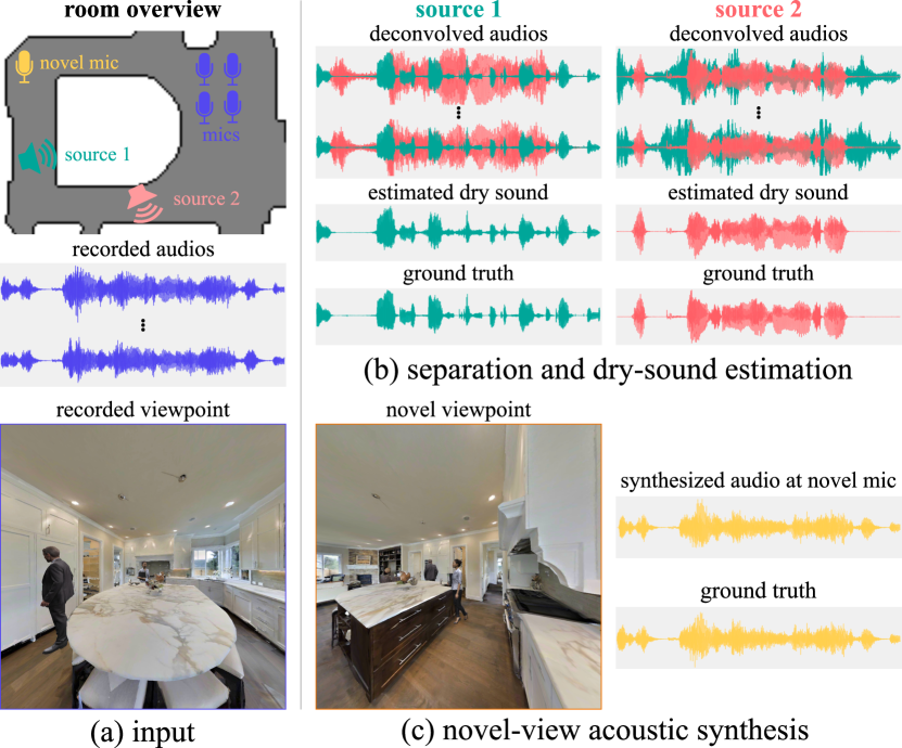
Fig. 2: Qualitative examples. (a) Receiver audio is recorded and (b) deconvolved with simulated RIRs. Leveraging the alignment from deconvolved audios, our method efficiently extracts dry sound, resulting in (c) synthesized audio from a novel viewpoint closely resembling true audio.

Novel-view acoustic synthesis

By localizing sound sources and estimating their dry sound, we effectively reconstruct the 3D acoustic scene. We subsequently resynthesize the audio anywhere in the scene using a standard renderer (SoundSpaces [10]). Our approach significantly outperforms ViGAS [5], which uses visual information and operates on single sound sources. Adding visual information further improves our results by boosting source detection accuracy and improving estimated dry sound (i.e., compare Ours v. Ours+visual). Fig. 2 shows waveforms of the results for dry sound estimation and novel-view acoustic synthesis. Our method effectively separates the dry sound from deconvolved audio and synthesizes novel-view audio consistent with ground truth. Video results are available at [1].

5 Conclusion

We introduced a method for novel-view acoustic synthesis which leverages advancements in 3D reconstruction and acoustic rendering. Our approach reconstructs an acoustic scene by jointly solving source localization, separation, and dereverberation, which allows us to realistically render immersive audio for users moving freely in a scene.

Limitations

We model sound sources as omni-directional point sources for simplicity. Our method relies on the availability of RIRs, and its performance can be influenced by the quality of the estimated RIRs.

Acknowledgement

We thank Dirk Schroeder and David Romblom for insightful discussions and feedback, Changan Chen for the assistance with SoundSpaces.

References

- [1] “Project page: Novel-view acoustic synthesis from 3d reconstructed rooms,” https://github.com/apple/ml-nvas3d, 2023.
- [2] B Mildenhall, PP Srinivasan, M Tancik, JT Barron, R Ramamoorthi, and R Ng, “Nerf: Representing scenes as neural radiance fields for view synthesis,” in ECCV, 2020.
- [3] Matthew Tancik, Ethan Weber, Evonne Ng, Ruilong Li, Brent Yi, Justin Kerr, Terrance Wang, Alexander Kristoffersen, Jake Austin, Kamyar Salahi, Abhik Ahuja, David McAllister, and Angjoo Kanazawa, “Nerfstudio: A modular framework for neural radiance field development,” in SIGGRAPH, 2023.
- [4] Jen-Hao Rick Chang, Wei-Yu Chen, Anurag Ranjan, Kwang Moo Yi, and Oncel Tuzel, “Pointersect: Neural rendering with cloud-ray intersection,” in CVPR, 2023.
- [5] Changan Chen, Alexander Richard, Roman Shapovalov, Vamsi Krishna Ithapu, Natalia Neverova, Kristen Grauman, and Andrea Vedaldi, “Novel-view acoustic synthesis,” in CVPR, 2023.
- [6] Carl Schissler, Christian Loftin, and Dinesh Manocha, “Acoustic classification and optimization for multi-modal rendering of real-world scenes,” TVCG, vol. 24, no. 3, 2017.
- [7] Anton Ratnarajah, Shi-Xiong Zhang, Meng Yu, Zhenyu Tang, Dinesh Manocha, and Dong Yu, “Fast-rir: Fast neural diffuse room impulse response generator,” in ICASSP, 2022.
- [8] Anton Ratnarajah, Zhenyu Tang, Rohith Aralikatti, and Dinesh Manocha, “Mesh2ir: Neural acoustic impulse response generator for complex 3d scenes,” in ACM International Conference on Multimedia, 2022.
- [9] Changan Chen, Unnat Jain, Carl Schissler, Sebastia Vicenc Amengual Gari, Ziad Al-Halah, Vamsi Krishna Ithapu, Philip Robinson, and Kristen Grauman, “Soundspaces: Audio-visual navigation in 3d environments,” in ECCV, 2020.
- [10] Changan Chen, Carl Schissler, Sanchit Garg, Philip Kobernik, Alexander Clegg, Paul Calamia, Dhruv Batra, Philip Robinson, and Kristen Grauman, “Soundspaces 2.0: A simulation platform for visual-acoustic learning,” NeurIPS, 2022.
- [11] Thomas Funkhouser, Ingrid Carlbom, Gary Elko, Gopal Pingali, Mohan Sondhi, and Jim West, “A beam tracing approach to acoustic modeling for interactive virtual environments,” in Conference on Computer graphics and interactive techniques, 1998.
- [12] Carl Schissler, Ravish Mehra, and Dinesh Manocha, “High-order diffraction and diffuse reflections for interactive sound propagation in large environments,” TOG, vol. 33, no. 4, 2014.
- [13] Ulf Michel, “History of acoustic beamforming,” in Berlin Beamforming Conference, 2006.
- [14] Zhenyu Tang, Nicholas J Bryan, Dingzeyu Li, Timothy R Langlois, and Dinesh Manocha, “Scene-aware audio rendering via deep acoustic analysis,” TVCG, vol. 26, no. 5, 2020.
- [15] Anton Ratnarajah and Dinesh Manocha, “Listen2scene: Interactive material-aware binaural sound propagation for reconstructed 3d scenes,” arXiv:2302.02809, 2023.
- [16] Andrew Luo, Yilun Du, Michael Tarr, Josh Tenenbaum, Antonio Torralba, and Chuang Gan, “Learning neural acoustic fields,” NeurIPS, 2022.
- [17] Miguel Sarabia, Elena Menyaylenko, Alessandro Toso, Skyler Seto, Zakaria Aldeneh, Shadi Pirhosseinloo, Luca Zappella, Barry-John Theobald, Nicholas Apostoloff, and Jonathan Sheaffer, “Spatial LibriSpeech: An Augmented Dataset for Spatial Audio Learning,” in Interspeech, 2023.
- [18] Simon Rouard, Francisco Massa, and Alexandre Défossez, “Hybrid transformers for music source separation,” in ICASSP, 2023.
- [19] Shentong Mo and Pedro Morgado, “A closer look at weakly-supervised audio-visual source localization,” NeurIPS, 2022.
- [20] Hang Zhao, Chuang Gan, Andrew Rouditchenko, Carl Vondrick, Josh McDermott, and Antonio Torralba, “The sound of pixels,” in ECCV, 2018.
- [21] Hang Zhao, Chuang Gan, Wei-Chiu Ma, and Antonio Torralba, “The sound of motions,” in ICCV, 2019.
- [22] Ariel Ephrat, Inbar Mosseri, Oran Lang, Tali Dekel, Kevin Wilson, Avinatan Hassidim, William T. Freeman, and Michael Rubinstein, “Looking to listen at the cocktail party: A speaker-independent audio-visual model for speech separation,” ToG, vol. 37, no. 4, 2018.
- [23] Daniel Michelsanti, Zheng-Hua Tan, Shi-Xiong Zhang, Yong Xu, Meng Yu, Dong Yu, and Jesper Jensen, “An overview of deep-learning-based audio-visual speech enhancement and separation,” IEEE/ACM Transactions on Audio, Speech, and Language Processing, vol. 29, 2021.
- [24] Changan Chen, Wei Sun, David Harwath, and Kristen Grauman, “Learning audio-visual dereverberation,” in ICASSP, 2023.
- [25] Sagnik Majumder and Kristen Grauman, “Active audio-visual separation of dynamic sound sources,” in ECCV, 2022.
- [26] Arun Asokan Nair, Austin Reiter, Changxi Zheng, and Shree Nayar, “Audiovisual zooming: what you see is what you hear,” in ACM International Conference on Multimedia, 2019.
- [27] Sharon Gannot, Emmanuel Vincent, Shmulik Markovich-Golan, and Alexey Ozerov, “A consolidated perspective on multimicrophone speech enhancement and source separation,” IEEE/ACM Transactions on Audio, Speech, and Language Processing, vol. 25, no. 4, 2017.
- [28] Heinz Teutsch, Modal array signal processing: principles and applications of acoustic wavefield decomposition, vol. 348, Springer, 2007.
- [29] Barry D Van Veen and Kevin M Buckley, “Beamforming: A versatile approach to spatial filtering,” IEEE assp magazine, vol. 5, no. 2, 1988.
- [30] Petre Stoica, Randolph L Moses, et al., Spectral analysis of signals, vol. 452, Pearson Prentice Hall Upper Saddle River, NJ, 2005.
- [31] Harry L Van Trees, Detection, estimation, and modulation theory: Part IV, John Wiley & Sons, Incorporated, 2002.
- [32] Ruohan Gao and Kristen Grauman, “Visualvoice: Audio-visual speech separation with cross-modal consistency,” in CVPR, 2021.
- [33] Norbert Wiener, “Extrapolation, interpolation, and smoothing of stationary time series, with engineering applications,” 1964.
- [34] Li Xu, Jimmy S Ren, Ce Liu, and Jiaya Jia, “Deep convolutional neural network for image deconvolution,” NeurIPS, 2014.
- [35] Angel Chang, Angela Dai, Thomas Funkhouser, Maciej Halber, Matthias Niessner, Manolis Savva, Shuran Song, Andy Zeng, and Yinda Zhang, “Matterport3d: Learning from rgb-d data in indoor environments,” 3DV, 2017.
- [36] Vassil Panayotov, Guoguo Chen, Daniel Povey, and Sanjeev Khudanpur, “Librispeech: an asr corpus based on public domain audio books,” in ICASSP, 2015.
- [37] Ethan Manilow, Gordon Wichern, Prem Seetharaman, and Jonathan Le Roux, “Cutting music source separation some Slakh: A dataset to study the impact of training data quality and quantity,” in WASPAA, 2019.
- [38] Emmanuel Vincent, Rémi Gribonval, and Cédric Févotte, “Performance measurement in blind audio source separation,” IEEE Transactions on Audio, Speech, and Language Processing, vol. 14, no. 4, 2006.
- [39] Scott Wisdom, Hakan Erdogan, Daniel PW Ellis, Romain Serizel, Nicolas Turpault, Eduardo Fonseca, Justin Salamon, Prem Seetharaman, and John R Hershey, “What’s all the fuss about free universal sound separation data?,” in ICASSP, 2021.