A Canonical Data Transformation for Achieving Inter- and Within-group Fairness

Abstract

Increases in the deployment of machine learning algorithms for applications that deal with sensitive data have brought attention to the issue of fairness in machine learning. Many works have been devoted to applications that require different demographic groups to be treated fairly. However, algorithms that aim to satisfy inter-group fairness (also called group fairness) may inadvertently treat individuals within the same demographic group unfairly. To address this issue, we introduce a formal definition of within-group fairness that maintains fairness among individuals from within the same group. We propose a pre-processing framework to meet both inter- and within-group fairness criteria with little compromise in accuracy. The framework maps the feature vectors of members from different groups to an inter-group-fair canonical domain before feeding them into a scoring function. The mapping is constructed to preserve the relative relationship between the scores obtained from the unprocessed feature vectors of individuals from the same demographic group, guaranteeing within-group fairness. We apply this framework to the COMPAS risk assessment and Law School datasets and compare its performance in achieving inter-group and within-group fairness to two regularization-based methods.

I Introduction

The deployment of machine learning (ML) models in sensitive domains—including criminal justice, healthcare, advertising, and the financial industry—are increasingly raising legal and ethical concerns [28]. In a number of studies, bias was detected in ML models that were used to make sensitive decisions; racial discrimination was detected in the COMPAS recidivism assessment model [4] and Google’s Ads model [30], gender discrimination was found in Amazon’s recruiting model [9], and skin tone bias was found in models used for melanoma detection from images [2]. Because the results produced by the models rely on the data on which they are trained, societal biases embedded in the data may be inherited by these models without proper intervention. There is a growing body of research focused on combating unfairness in ML models from which a number of definitions of fairness have been advanced and many tools have been developed for achieving them. Two of the most prominent categories of fairness definitions that have been studied include: (1) group fairness [15, 8, 7, 12, 20, 5, 21] and (2) individual fairness [11, 24, 18, 13, 19, 17, 29]. Group fairness definitions focus on ensuring that different demographic groups of the population are treated equally, while individual fairness definitions aim to guarantee that individuals with similar feature values are treated similarly.

As multiple works have shown [8, 23, 35], achieving a universal notion of fairness is impossible. When it is desirable to satisfy multiple conflicting notions of fairness, compromises must be made. Taking the loan approval decision process as an example, it is illegal under fair lending laws to discriminate against people based on protected attributes including, but not limited to, race, sex, and religion [1]. In particular, financial institutions are required to conduct bias assessments to prove that they are engaged in fair lending practices that are not biased against such groups [6].

Multiple approaches could be deployed to ensure that group-based fairness is preserved. For example, separate scoring thresholds could be applied to different groups to offset biases reflected in the scoring distributions produced by a model or the output scores of different groups could be equalized using a post-processing transformation. Yet in many situations knowledge of sensitive features is prohibited from being directly used in the decision-making process in the testing stage, disqualifying such approaches. Another approach could be to enforce group fairness in the model by incorporating regularization into the training process. However, a lack of heterogeneity among the feature values of individuals within a group may impede a learned model from equalizing the scoring distributions across different groups without disparately impacting similar individuals within a group. Hence, asking a classifier to approximate statistical parity between different groups may cause it to badly violate parity among the individuals within a group [22]. This highlights an important consideration in dealing with problems in which group fairness is a hard constraint—solutions to such problems should still treat individuals within each group fairly with respect to each other. In the remainder of this paper, we will use the terminology inter-group fairness in place of group fairness to avoid any potential confusion between this notion and the notion of within-group fairness.

Our goal in this work is to introduce a prepossessing framework for maintaining individual fairness within each group in situations where group fairness is a requirement and sensitive attributes are not allowed to be used for decision-making in the testing stage of the ML process. The core idea of the our pre-processing framework is to devise a mapping that preserves fairness among individuals while mapping the data from each group associated with a sensitive feature to a canonical data domain that is blind to the sensitive attribute itself. We adopt a stringent notion of fairness—the threshold invariant form of demographic parity [20]—for our inter-group fairness definition [7] and introduce a new definition of within-group fairness, which is used to devise measures for fairness assessment. We compare this approach against a regularization-based training procedure for comparison.

The remainder of this paper is organized as follows. In Section II, a summary of basic fairness-related concepts relevant to this work is provided. In Section III, the problem setup is formulated, while in Section IV, the prepossessing framework is described along with the regularized training approach used for comparison. Experimental results are presented in Section V to quantify each method’s accuracy and ability to achieve inter-group fairness, and within-group fairness. Finally, the paper is concluded in Section VII.

II Background and Related Work

Fairness definitions

Fairness definitions may be categorized into three main types, including the inter-group, individual, and subgroup fairness [27]. Inter-group fairness is measured by the prediction performance parity across different demographic groups. To deal with multifaceted bias and discrimination issues, there are various notions proposed including demographic parity [11], equalized odds [15], test fairness[8], and threshold invariant fairness [7]. Guaranteeing only inter-group fairness is insufficient as there are cases, from the perspective of an individual, where the outcome is blatantly unfair even if inter-group fairness is satisfied [34]. Individual fairness aims to give similar prediction performance for similar individuals with respect to the same task [11]. To bridge the gap between inter-group fairness and individual fairness, Kearns et al. [22] proposed subgroup fairness. Subgroup fairness applies the inter-group fairness constraint on a large collection of subgroups defined over combinations of protected attribute values.

In this paper, we define another fairness notion—within-group fairness. Within-group fairness aims to preserve the relative relationship between the scores of individuals from the same demographic group before and after inter-group fairness is accounted for. This idea is related to the sub-group fairness definition produced by Kearns et al. [22] in the special case where each individual in a group is considered a sub-group.

Design of fairness-aware algorithms

Given various fairness definitions and criteria, many methods have been studied to achieve fairness in machine learning, which can be categorized accordingly: (1) pre-processing, (2) inprocessing, and (3) post-processing [27]. Pre-processing approaches aim to modify or transform the training data to remove underlying biases. Kamiran et al. [20] proposed a pre-processing method by “massaging” the training labels to remove the discrimination. In their method, a ranker is used to select which labels to change while minimizing the impact on the prediction accuracy. Inprocessing methods introduce fairness-aware regularizers into the objective function during the training process, which aim to balance between maximizing accuracy and minimizing unfairness [21]. Calders et al. [5] devised a regularizer that enforces the trained classifier to be independent of the sensitive attribute, while Zafar et al. [33, 32] enforce demographic parity and equalized odds constraints in the classifier training process. Chen et al. [7] designed a fairness loss that aims to equalize the score distributions from different demographic groups. The third method, post-processing, achieves fairness by reassigning the scores produced by the initial black-box model using a function after training [12]. Other post-processing methods can mitigate bias [26] by identifying unfair features via attention mechanisms and manipulating the corresponding attention weights.

In this paper, we propose a pre-processing method where the feature vectors from different demographic groups are mapped into a canonical distribution in which within-group fairness is achieved.

III Problem Setup

III-A Notation

Following Dwork et al., we refer to individuals as the objects that we aim to classify [11]. We refer to the set of individuals as $\mathcal{I}$. Each individual, $i\in\mathcal{I}$, has a corresponding feature vector, $\mathbf{f}_{i}\in\mathbb{R}^{k}$, the elements of which represent values associated with features from the feature set, $\mathcal{F}\triangleq\{f_{1},\ldots,f_{k}\}$. We refer to a subset of features, $\mathcal{A}\subseteq\mathcal{F}$ as sensitive if we are prohibited from discriminating against individuals based on the values of these features. Thus, no sensitive feature values are included in feature vectors. Each individual also has a label, $y\in\{0,1\}$, associated with him or her. A dataset of $N$ individuals, $X\in\mathbb{R}^{N\times k}$, is a matrix in which each row represents an individual’s feature vector. The primary task of the binary classification problem is to predict the labels of individuals using a scoring function trained on a dataset. A scoring function, $s_{\boldsymbol{\theta}}:\mathbb{R}^{k}\to[0,1]$, is defined as a mapping of a feature vector to a score between $0$ and $1$, inclusive. Given a threshold, $t$, the estimator associated with a scoring function, $s_{\boldsymbol{\theta}}$, is represented by the function:

$$\hat{Y}=\begin{cases}0,&s_{\boldsymbol{\theta}}(\mathbf{f})\leq t\\ 1,&s_{\boldsymbol{\theta}}(\mathbf{f})>t,\end{cases}$$ (1)

and is used to predict the label associated with a given individual. A scoring function is trained on data to optimize its parameters to satisfy an objective and tested on separate data to ensure the results it produces are generalizable. We refer to the training dataset as $\mathbf{X}_{tr}$ and the testing dataset as $\mathbf{X}_{ts}$. A loss function, $L_{\boldsymbol{\theta}}$, is used to quantify the ability of the scoring function to produce scores that satisfy the objective. A learning algorithm optimizes the weights of the scoring function, $\boldsymbol{\theta}$, according to $L_{\boldsymbol{\theta}}$.

A group, $g\subseteq{\mathcal{I}}$, is a collection of individuals that share the same values for the sensitive features in $\mathcal{A}$. The set of all groups is denoted $\mathcal{G}$. We use numerical superscripts to specify group membership. For example, $X^{(i)}$ refers to the subset of the dataset $X$ belonging to group $i$. The omission of superscripts indicates that we are referring to population information. Lastly, $d_{\mathcal{X}}$ represents a distance measure over the set $\mathcal{X}$.

III-B Inter-group Fairness

A variety of definitions have been proposed regarding inter-group fairness. Two of the most common ones include demographic parity (DP) and equalized odds (EO), and we focus on DP in this paper.

Definition 1.

(Demographic Parity) An estimator, $\hat{Y}$, satisfies demographic parity for a binary feature, $A\in\{0,1\}$, if $P(\hat{Y}=1|A=0)=P(\hat{Y}=1|A=1)$.

An important observation to make about this definitions is that it is threshold dependent. That is, a particular classifier may achieve DP for a given threshold, but not for all thresholds in the range $[0,1]$, when the distributions of the scoring function associated with different groups deviates. In many applications, this may lead to privacy issues. For example many financial institutions develop ML teams for automating the loan decision making process and compliance teams for overseeing sensitive data. Since the ML team is not allowed to access any sensitive information associated with the data, privacy concerns arise if the output scoring distributions are not equal across groups. Thus, we wish to ensure that the scoring distributions are equal across groups. This intuition is encapsulated in the more strict definition of threshold-invariant fairness defined by Chen et al. [7]. Thus, we use this definition for the inter-group fairness notion for our analysis:

Definition 2.

(Threshold Invariant Fairness) Threshold Invariant Demographic Parity (TIDP) is achieved when DP is satisfied, independent of the decision threshold t.

To measure how well a classifier preserves TIDP, we can take the average of the Calder-Verwer (CV) score [5] for every possible threshold value $t$, where the CV scores for DP are given by: $\Delta_{DP}=|P(\hat{Y}=1|A=0)-P(\hat{Y}=1|A=1)|$. The framework that we propose in this paper aims to achieve TIDP, while maintaining within-group fairness.

III-C Within-group Fairness

In the previous subsection, we discussed measures of inter-group fairness, which are blind to the treatment individuals. To understand the negative side-effects that may arise from only taking inter-group fairness into account, we provide the following simple motivating example.

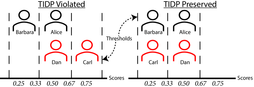
Figure 1: Fairness Example 1 illustration.

Example 1.

Consider four individuals, Alice and Barbara, who are female, and Carl and Dan, who are male. Assume that all other sensitive attributes are the same for all individuals. According to the information in their loan applications, they receive the following loan approval scores, respectively: 0.50, 0.25; 0.75, 0.50. Since the distribution of scores between the male and female groups is different, a loan officer adjusts Carl’s score to a value of 0.25 so that TIDP-based inter-group fairness is satisfied since for any threshold, the same number of individuals for each sex scores above it. (see Figure 1). However, assuming all applicants were scored according only to non-sensitive features, we see that Carl’s outcome is unfair since he has a stronger application than Dan.

This simple example highlights an important consideration which must be taken into account in the fairness process: individual fairness must still be preserved within each group. Clearly, a more individually fair way to achieve TIDP in Example 1 would be to provide Carl with a score of 0.50 and Dan with a score of 0.25. Thus, we introduce a new definition, within-group, fairness which takes advantage of the insight provided in this example—the most accurate scores assigned to individuals are the fairest to individuals that belong to the same group. This suggests that the scores provided by a baseline model, which does not explicitly account for any notion of fairness, yield the fairest scores when comparing individuals within the same group.

The inspiration for our definition comes from Dwork et al.’s definition of individual fairness, which states that similar individuals should be treated similarly [11], and we adapt the definition according to the notation of our problem below.

Definition 3.

(Individual Fairness) A scoring function $s:\mathbb{R}^{k}\to[0,1]$ satisfies individual fairness if for any two individuals $i,j\in\mathcal{I}$, $|P(\hat{Y}_{i}=y)-P(\hat{Y}_{j}=y)|\leq\epsilon;\ \ \ \ \ if\ \ d_{\mathcal{I}}(i,j)\approx 0$.

With this in mind, we provide a few definitions that build toward our definition of within-group fairness.

Definition 4.

(Signed Distance Function) The signed distance function for $x,y\in\mathcal{X}$ is given by:

$$\phi_{\mathcal{X}}(x,y)=\begin{cases}d_{\mathcal{X}}(x,y),&x\leq y\\ -d_{\mathcal{X}}(x,y),&x>y\end{cases}$$ (2)

Definition 5.

(Individual Fairness Across Mappings) A mapping $Q:\mathbb{R}^{k}\to[0,1]$ satisfys individual fairness with respect to a different mapping $R:\mathbb{R}^{k}\to[0,1]$ if for any two individuals, $i,j\in\mathcal{I}$,

$$|\phi_{[0,1]}(Q(\mathbf{f}_{i}),Q(\mathbf{f}_{j}))-\phi_{[0,1]}(R(\mathbf{f}_{i}),R(\mathbf{f}_{j}))|\leq\epsilon.$$ (3)

Definition 6.

(Within-group Fairness Across Mappings) A mapping $Q:\mathbb{R}^{k}\to[0,1]$ is said to satisfy within-group fairness with respect to a different mapping $R:\mathbb{R}^{k}\to[0,1]$ if for any group $g\in\mathcal{G}$, individual fairness across models is satisfied between any two individuals, $i,j\in g$. That is,

$$|\phi_{[0,1]}(Q(\mathbf{f}_{i}),Q(\mathbf{f}_{j}))-\phi_{[0,1]}(R(\mathbf{f}_{i}), R(\mathbf{f}_{j}))|\leq\epsilon,$$

$$\forall g\in\mathcal{G};\forall i,j\in g$$ (4)

Intuitively, our within-group fairness definition states that the scores provided by one mapping are fair with respect to another if the distance between any two individuals’ scores is relatively preserved and the ordering of their scores does not change across models. In the algorithm proposed in Section IV, we consider one of the mappings to be the baseline trained scoring function. The second mapping is considered to be a pre-processing transformation $T:\mathbb{R}^{k}\to\mathbb{R}^{k}$ composed with the baseline trained scoring function. $T$ is applied to map the feature vectors of individuals from different groups to a canonical inter-group-fair domain. Thus, if Definition 6 is satisfied, then our framework achieves both inter-group and within-group fairness.

To quantify how well a mapping, $Q$, is able to preserve within-group fairness with respect to another mapping, $R$, we can calculate the percentage of pairs of individuals in a dataset whose scoring relationships are not preserved across models. Specifically, the following measure can be used to quantify within-group fairness:

$$\Delta_{WGF}=$$

$$\frac{2\sum_{g\in\mathcal{G}}\sum_{\begin{subarray}{c}i,j\in g\\ i<j\end{subarray}}\mathbf{1}\{|\phi(Q(\mathbf{f}_{i}),Q(\mathbf{f}_{j}))-\phi(R(\mathbf{f}_{i}),R(\mathbf{f}_{j}))|>\epsilon\}}{\sum_{g\in\mathcal{G}}N_{g}(N_{g}-1)},$$ (5)

where $\mathbf{1}$ represents the indicator function, $\epsilon$ may be a user-specified parameter quantifying how much within-group unfairness we are willing to tolerate, and $N_{g}$ is the number of individuals in group $g$.

IV Framework for Achieving Group and Within-group Fairness

In this section we outline the proposed pre-processing framework for achieving inter- and within-group fairness. We also describe an in-processing algorithm in which fairness is encouraged through the loss function during training with the use of regularizers, which we use to compare against our framework.

IV-A Proposed Pre-processing Framework

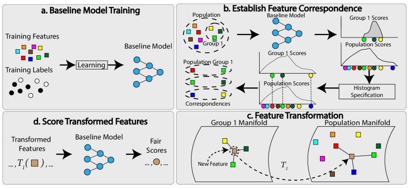
Figure 2: Overview of the pre-processing framework for achieving inter- and within-group fairness.

Figure 2 illustrates the pre-processing algorithm. The goal is to design these mappings, such that when the baseline scoring function is applied to the transformed feature vectors of any group, the output scoring distribution will resemble the original un-transformed population scoring distribution. The transform is constructed by creating a correspondence between feature vectors in each group to feature vectors in the entire population. The details of each phase of the system are presented in the ensuing subsections.

Phase I: Baseline Model Training

Assume we have a population training dataset, $\mathbf{X}_{tr}\in\mathbb{R}^{N_{tr}\times k}$ with associated labels $\mathbf{y}\in\{0,1\}^{N_{tr}}$ consisting of $N_{tr}$ individuals. We construct a scoring function of the form $s_{\boldsymbol{\theta}}(x)=\sigma(m_{\boldsymbol{\theta}}(x))$, where $m_{\boldsymbol{\theta}}:\mathbb{R}^{k}\to\mathbb{R}$ is an ML model (e.g. logistic regression, support vector machine, neural network, etc.) and $\sigma:\mathbb{R}\to[0,1]$ is the sigmoid function. We call this scoring function the baseline model. The baseline model is designed to maximize accuracy according to the training data using a standard (sub-)differentiable loss function, $L_{\boldsymbol{\theta}}$, (e.g., cross-entropy, hinge, etc.). Finally, a learning algorithm (e.g., gradient descent, stochastic gradient descent, etc.) to optimize the model weights, $\boldsymbol{\theta}$.

Phase II: Establish Feature Correspondence

Once the baseline model, $s_{\boldsymbol{\theta}}$, is obtained from Phase I, we split the population training data according to the groups to which each individual belongs, where we assume these groups are mutually exclusive. Specifically, we decompose $\mathbf{X}_{tr}$ into group training datasets $\mathbf{X}_{tr}^{(i)},i=1,\ldots,|\mathcal{G}|$. The baseline model is applied to each group training dataset and the population training dataset to obtain the score vectors $\mathbf{s}_{tr}^{(i)},i=1,\ldots,|\mathcal{G}|$ and $\mathbf{s}_{tr}$, respectively. We then perform histogram specification [14] to map the distribution of scores associated with each group to the population score distribution. We denote these score vectors by $\hat{\mathbf{s}}_{tr}^{(i)},i=1,\ldots,|\mathcal{G}|$. Because the scores in $\hat{\mathbf{s}}_{tr}^{(i)}$ and $\mathbf{s}_{tr}$ are approximately equally distributed, each score in $\hat{\mathbf{s}}_{tr}^{(i)}$ should be close in distance to some score in $\mathbf{s}_{tr}$. We pair group and population feature vectors if their scores are sufficiently close, calling such pairs feature correspondences.

Definition 7.

(Feature Correspondence) Let $a\in\hat{\mathbf{s}}_{tr}^{(i)}$ and $b\in\mathbf{s}_{tr}$ be the scores associated with the $n^{th}$ feature vector of group $i$, $\mathbf{f}_{n}^{(i)}$, and the $l^{th}$ feature vector of the population $\mathbf{f}_{l}$. We say $\mathbf{f}_{n}^{(i)}$ and $\mathbf{f}_{l}$ form a correspondence, denoted $\mathbf{f}_{n}^{(i)}\sim\mathbf{f}_{l}$, if for any $c\in\mathbf{s}_{tr}$, such that $c\neq b$, the following inequality holds $|a-b|\leq|a-c|$.

Our goal is to exploit these feature correspondences to create a transformation that maps feature vectors from each group to the canonical population domain. This idea is illustrated in Figure 2b. Critically, histogram specification is a monotonically increasing transform on the scores. As a result, when we use these correspondences to construct our group transformations, they should preserve the ordering of the points produced by the baseline model on their $original$ feature vectors, thereby preserving our notion of within-group fairness.

Phase III: Mapping Construction

Phase III uses the feature correspondences found in Phase II to construct a mapping between each group domain and the population domain for individuals not seen in the training data. Our approach assumes that each group’s data lie on a manifold in $\mathbb{R}^{k}$ and that the training data sample this manifold densely enough to provide a faithful representation of it. Hence our goal is to construct a more general correspondence between each group’s manifold to the population manifold. To achieve this goal, we turn to computational geometry, taking advantage of the structural properties of the $k$-$d$ tree. The $k$-$d$ tree is a space-partitioning data structure used to organize points in k-dimensional space. In this data structure, each leaf node represents one datapoint, while each non-leaf node represents a splitting hyperplane used to generate two half spaces. The points in each half space correspond to the leaves of a given node’s subtree. This structure is illustrated in Figure  3. The $k$-$d$ tree has a particularly important property that we exploit—it can be used to efficiently perform nearest neighbor searches for data in high dimensions. Using this property, we represent new feature vectors as a weighted combination of their closest neighboring training feature vectors in $\mathbb{R}^{k}$. Specifically, we construct $|\mathcal{G}|$ $k$-$d$ trees using the feature vectors in the training sets $\mathbf{X}_{tr}^{(i)},i=1,\ldots,|\mathcal{G}|$ to represent each group’s individual manifold. When a new feature vector, $\mathbf{f}^{(i)}_{new}$ for group $i$, is to be pre-processed, we can represent it by a weighted average of feature vectors to which it is closest, as illustrated in Figure 2c, which are obtained by efficiently traversing the tree to find the closest neighbors to this new point.

Mapping new feature vectors from the group domain to the population domain can be done as follows. Without loss of generality (WLOG), let $\{\mathbf{f}_{n}^{(i)}\}_{n=1}^{k}$ represent the $k$ nearest neighbors of $\mathbf{f}^{(i)}_{new}$, belonging to group $i$. The Euclidean distances between $\mathbf{f}^{(i)}_{new}$ and the elements of $\{\mathbf{f}_{n}^{(i)}\}_{n=1}^{k}$ are represented by $\{d_{n}^{(i)}\}_{n=1}^{k}$. Inspired by the algorithm presented by Dongsheng et al. [3], we construct a set of weights $\{{d_{n}^{(i)-1}}/{\sum_{l=1}^{k}d_{l}^{(i)-1}}\}_{n=1}^{k}=\{w_{n}^{(i)}\}_{n=1}^{k}$ associated with each element in $\{\mathbf{f}_{n}^{(i)}\}_{n=1}^{k}$ that reflect how closely they resemble the new feature vector in the group domain. In the population domain, WLOG, we obtain the corresponding feature vectors $\{\mathbf{f}_{n}\}_{n=1}^{k}$, where $\mathbf{f}^{(i)}_{n}\sim\mathbf{f}_{n}$, and use these weights to construct their new feature vectors in the population domain $\mathbf{f}_{new}=\sum_{l=1}^{k}w_{l}f_{l}$. We use the notation $T^{(i)}:\mathbb{R}^{k}\to\mathbb{R}^{k}$ to describe the mapping from a feature vector from group $i$’s domain to the population domain. Hence, given a test dataset, $\mathbf{X}_{ts}\in\mathbb{R}^{N_{ts}\times k}$ of $N_{ts}$ individuals, we can decompose it in group test sets $\mathbf{X}_{ts}^{(i)},i,...,|\mathcal{G}|$, obtain the canonical group test dataset, $T^{(i)}(\mathbf{X}_{ts}^{(i)}),i,...,|\mathcal{G}|$, and apply the baseline model, $s_{\boldsymbol{\theta}}$, to it. A user-specified threshold, $t$, can then be used to make the classification decision for these test data.

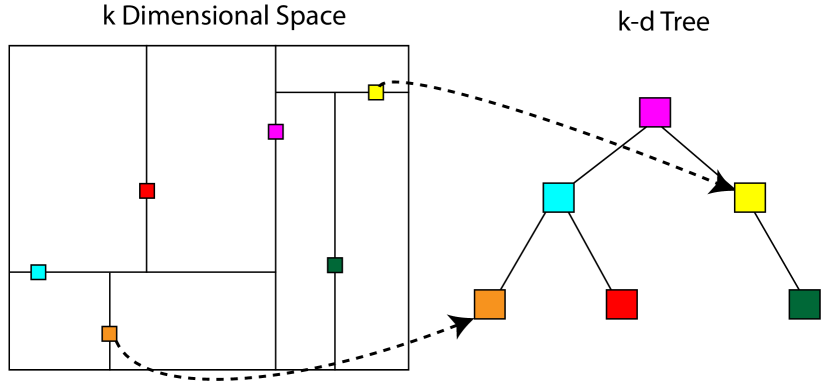
Figure 3: Representation of a $k$-$d$ tree.

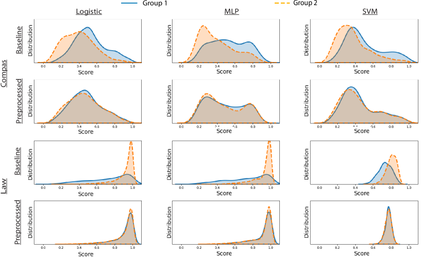
Figure 4: The distribution of scores produced by the baseline scoring function (top row) and the pre-processing framework (bottom row) for using three different ML models.

IV-B In-processing Framework

In this section we describe an in-processing alternative to our pre-processing framework for comparison. In this approach, a scoring function is trained to internalize inter-group fairness in the training process. This approach is similar to that of the algorithm described by Chen et al. [7].

We start by training a baseline scoring function, $s_{\boldsymbol{\theta}}(x)$, as in Phase I of Section IV-A. The weights $\boldsymbol{\theta}$ serve as a starting point from which we will fine-tune to improve the fairness of the scoring function. Specifically, once we obtain

$$\boldsymbol{\theta}^{base}=\underset{\boldsymbol{\theta}}{\arg\min}\ L_{\boldsymbol{\theta}}(\mathbf{X}_{tr}),$$ (6)

We learn another set of weights, $\boldsymbol{\theta}^{eq}$, for $s_{\boldsymbol{\theta}}(x)$ through

$$\boldsymbol{\theta}^{eq}=\underset{\theta}{\arg\min}\ L_{\boldsymbol{\theta}}(\mathbf{X}_{tr})+\lambda E(\mathbf{X}_{tr}),$$ (7)

by initializing $\boldsymbol{\theta}=\boldsymbol{\theta}^{base}$ before applying the learning algorithm. Here, $E(\mathbf{X}_{tr})$, is a regularizer that uses a distance notion to calculate the distance between the scores from two different groups, $i,j\in\mathcal{G}$. We take this two-stage fine-tuning approach instead of directly optimizing Equation 7 starting from random weights for two reasons. First, by using $\boldsymbol{\theta}^{base}$ as our starting point, we are able to start at the most accurate solution and observe the trade-off we incur between inter-group fairness and accuracy during the training process in 7. Second, training the scoring model using Equation 7 with a randomized initialization of $\boldsymbol{\theta}$ can lead to instability in the resulting output of $\boldsymbol{\theta}^{eq}$ reflected by the random seed from which $\boldsymbol{\theta}$ is initialized.

Two common regularizers are considered to compare with our pre-processing framework: (1) an Earth Mover’s distance (EMD) regularizer [16] and (2) a Kullback–Leibler (KL) divergence regularizer. The EMD regularizer is of the form:

$$EMD(\mathbf{X}_{tr}^{(i)},\mathbf{X}_{tr}^{(j)})=\sum_{n=1}^{C}(CDF_{n}(\hat{\mathbf{h}}_{i})-CDF_{n}(\hat{\mathbf{h}}_{j}))^{2},$$ (8)

where CDF represents the cumulative distribution function, $n$ represents the energy in the $n^{th}$ bin of the CDF, and $\hat{\mathbf{h}}_{i}$ and $\hat{\mathbf{h}}_{j}$ are Gaussian approximated histogram bins calculated from $\mathbf{X}_{tr}^{(i)}$ and $\mathbf{X}_{tr}^{(j)}$. Because rectangular histogram bins are non-differentiable at the bin edges, we use Gaussian approximations of the rectangular histogram bins as done by Chen et al. [7] so that we can apply a (sub-)gradient-based learning algorithm for optimizing $\boldsymbol{\theta}$.

For the second regularizer tested, we use the symmetric KL divergence with an added Gaussian assumption that Chen et al. [7] formulate. Since the KL divergence is less tractable than the EMD, using the aforementioned Gaussian approximated histogram binning approach leads to convergence issues when trying to equalize group distributions. Adding the Gaussian assumption instead leads to a simple loss that is only dependent on the second order statistics of each group dataset, alleviating these tractability issues. Thus, letting $\mathcal{N}_{i}$ and $\mathcal{N}_{j}$ represent normal distributions with the same mean and variance as group $i$ and group $j$, respectively, the regularizer is given as:

$$KL (\mathbf{X}_{tr}^{(i)},\mathbf{X}_{tr}^{(j)})$$

$$=\frac{1}{2}(\frac{(\hat{\mu}_{i}-\hat{\mu}_{j})-\hat{\sigma}_{i}}{\hat{\sigma}_{j}}+\frac{(\hat{\mu}_{j}-\hat{\mu}_{i})-\hat{\sigma}_{j}}{\hat{\sigma}_{i}})-2.$$ (9)

V Experimental Results

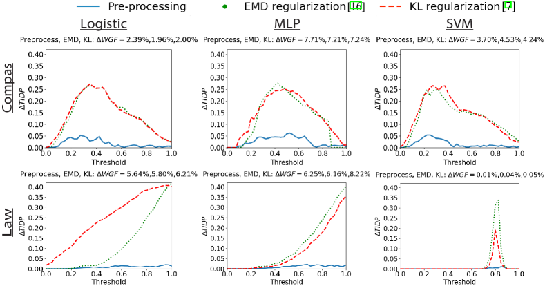
Figure 5: Plots $\Delta_{TIDP}$ at different thresholds when a specified when an average $\Delta_{WGF}$ value has been achieved for three different models: (a) Logistic Regression, (b)MLP, and (c) SVM.

TABLE I: Dataset Compositions

Characteristic	COMPAS	Law
Features	age sex juv_fel_count juv_misd_count juv_other_count priors_count c_charge_degree	decile1b decile3 lsat ugpa zfygpa zgpa fulltime family income sex tier
Class Label	Recividate (0/1)	Pass Bar (0/1)
Sensitive attribute	Race (White/Black)	Race (White/Non-white)
# Samples (Group 1/Group 2)	2103/3175	17491/3307
# 0/1 Class Labels (Group 1)	822/1281	1377/16114
# 0/1 Class Labels (Group 2)	1514/1661	916/2391

In this section, the pre-processing framework is analyzed on the COMPAS risk assessment [25] and Law School [31] datasets—two benchmark datasets with known biases with respect to a given sensitive attribute. For brevity, we simply refer to these datasets as the COMPAS and Law datasets. The COMPAS dataset is composed of the records of criminal defendants screened by the COMPAS model in Broward County. It includes information on a defendant’s demographics, case details, and criminal histories, with the ML task being to use this information to predict whether a person recidivated within two years of being screened. Biases have been found to exist in the score distributions of white and black demographic groups produced by ML models trained on this dataset, with the white demographic group having lower scores than the black demographic group on average. The Law dataset contains law school admissions records from a survey conducted by the Law School Admission Council (LSAC) across 163 law schools in the United States in 1991. Using the variables provided in this dataset, the ML task is to predict whether someone is likely to pass the bar exam or not. ML models trained on this dataset have been shown to produce biased score distributions when predicting whether white and non-white demographic groups will pass the bar examination, with the white demographic group having much higher scores on average.

In Table I we provide details on the composition of each dataset used for training and testing the models in our experiments. A full description of each feature in the dataset is provided in Tables V and VI of the appendix. Group 1 and Group 2 respectively refer to the advantaged and disadvantaged groups in both datasets. It can clearly be observed that bias exists in the class label distributions associated with each group. We also note that 0 and 1 class labels associated with each dataset have opposing connotations. For the COMPAS, a 1 class label indicates that a person did recividate, while for the Law dataset, a 1 class label indicates that a person passed the bar examination. Moreover, in the COMPAS dataset, the minority group (Group 1) is advantaged, while the opposite is the case in the Law dataset. Thus, there is diversity in the distributions associated with each dataset, which is good for drawing generalized insights from our results.

The ensuing subsections are devoted to testing the ability of the pre-processing framework to achieve both inter- and within-group fairness on both of these datasets. We compare its performance with the regularization approaches described in Section IV-B. As done by Chen et al. [7], we split all data into 70% training and 30% and make the simplifying assumption that race is the only binary sensitive attribute that creates inter-group unfairness in the data. All binary and categorical variables were one-hot-encoded and all ML models were trained in TensorFlow using gradient descent with step sizes between 0.01 and 0.001. All programs were conducted using Python 3.8 and run on a Macbook Pro (1.7 GHz Quad-Core Intel Core i7) with no GPU support. We used the SciPy library for $k$-$d$ tree construction and set $k=10$ for the number of nearest neighbors used in constructing the mappings from the group to population domain for all experiments.

V-A Baseline vs. Pre-processing Framework: Risk Distribution Comparison

In this section, the risk score distributions produced by the baseline scoring function and the pre-processing framework are visually compared for three different scoring functions: a Logistic regression (LR), three-layer perception (MLP), and support vector machine (SVM). These distributions are presented in Figure 4, with the first and second row corresponding to the COMPAS dataset and the third and fourth rows corresponding to the Law dataset. The first and third rows of distributions capture the baseline scoring function results applied to the raw feature vectors for the COMPAS and Law datasets, respectively. The second and fourth row of distributions use the preprocessing framework to map the raw feature vectors to the canonical population domains of the COMPAS and Law datasets, respectiviely, before applying their baseline scoring functions. The dark, overlapped regions in these plots capture the similarity between the distributions of Group 1 and 2. A classifier that perfectly captures TIDP would produce entirely overlapped distributions. It can clearly be seen that distributions associated with the pre-processed features show significantly more overlap than those associated with the raw features for each model for both datasets. Notably, the bias incurred between both groups in the risk distributions associated with the raw features is alleviated with the use of canonical features. Hence, these illustrations capture the improvements made in inter-group fairness by applying the baseline scoring function to the canonical features instead of to raw features.

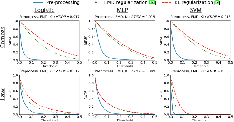
Figure 6: Plots $\Delta_{WGF}$ at different thresholds when a specified when an average $\Delta_{TIDP}$ value has been achieved for three different models: (a) Logistic Regression, (b)MLP, and (c) SVM.

V-B Pre-processing Framework vs. Regularization Methods

In this section, the pre-processing framework’s ability to achieve inter-group and within-group fairness is compared against the two regularization methods described in Section IV-B. The regularization methods are able to achieve different levels of fairness through the tuning of the weight placed on regularizer $\lambda$. In contrast, our pre-processing framework achieves a single-level of fairness since it involves no hyperparameters. Therefore, we aim to compare these approaches through addressing the following questions: (1) How much inter-group fairness does a regularization method give up in order to achieve the same level of within-group fairness as the pre-processing framework? (2) How much within-group fairness does a regularization method give up in order to achieve the same level of within-group fairness as the pre-processing framework?

We approach the first question as follows. Let $\Delta^{pre}_{WGF}$ represent the value of the within-group fairness measure produced by the pre-processing method on average for thresholds between 0 and 0.5. Let $\Delta^{reg}_{WGF}$ represent the value of the within-group fairness measure associated with a regularization method on average for thresholds between 0 and 0.5. We choose $\lambda$ in Equation IV-B such that $\Delta^{reg}_{WGF}\approx\Delta^{pre}_{WGF}$. Given that the pre-processing framework and regularization method achieve approximately the same level of within-group fairness, the method that achieves a higher level of inter-group fairness is better at achieving overall fairness. The second question is approached in the reverse direction. That is, we choose $\lambda$ such that the average amount of inter-group fairness achieved by both models is equal and then we compare their levels of within-group fairness.

The results of our comparative analysis are summarized in Figure 5 and Figure 6 for the COMPAS and Law testing data. Figure 5 displays plots of the within-group fairness measure, $\Delta_{WGF}$ for the pre-processing framework and both regularization methods for three different ML models. The value of $\Delta_{TIDP}$ above each plot represents the average value of the inter-group fairness measure associated with a particular method. It can clearly be seen that the average $\Delta_{TIDP}$ associated with the regularization methods are approximately equal to those of the pre-processing framework for both datasets. Regardless of the ML model, our pre-processing framework is able to achieve much lower values $\Delta_{WGF}$ for a wide range of thresholds for both datasets, indicating that fewer pairs of individuals in the pre-processing framework violate within-group fairness.

Figure 6 displays plots of the inter-group fairness measure, $\Delta_{TIDP}$ for the pre-processing framework and both regularization methods for three different ML models. The value of $\Delta_{WGF}$ above each plot represents the average value of the within-group fairness measure associated with a particular method. Again, for approximately equal values of the average $\Delta_{WGF}$ measure, the pre-processing framework consistently provides significantly lower $\Delta_{TIDP}$ values for all models and thresholds for both datasets. Thus, the results in Figures 5 and 6 indicate that the regularization methods must compromise between inter-group and within-group fairness, in contrast to our pre-processing framework.

V-C Accuracy Evaluation of Pre-processing Framework

In this section, we analyze the performance of our pre-processing framework. Applying the baseline classifier to the raw training features should produce the best results. However, the performance of a fair model should not be reduced significantly if it is to be considered useful in practice. Thus, we use two metrics—accuracy and area under the curve (AUC) for the receiver operating characteristic (ROC) curve—to compare the performances of the pre-processing framework and regularization methods that achieve approximately equal levels of group fairness to the baseline classifier’s performance. To analyze the accuracy of a method we use a value of 0.5 as the threshold for all classifiers, since this is the most common value used in practice. The resulting performances of these methods on the COMPAS and Law test data are shown in Tables IV and  III. The results in both tables show that the pre-processing framework outperforms the regularization-based methods. Compared with the baseline model, no more than a 2.78% in accuracy and 0.022 drop in AUC is incurred by any of the three ML models when applying the pre-processing framework to the COMPAS dataset. In contrast, when applying the regularization methods to the COMPAS dataset, we see accuracy drop-offs of over 8.91% and AUC dropoffs of over 0.100 in all cases. Though, the pre-processing framework also outperforms the regularization approaches on the Law dataset, the results are less pronounced. That is, all methods incur little drop in accuracy from the baseline model. This is because the there is large class imbalance for this dataset, with 88.97% of the class labels in this dataset having a value of 1. Thus, simply assigning everyone the same class label will achieve a high accuracy. On the other hand, the AUC for the ROC curve shows much more significant dropoffs in the results obtained for the regularization methods than the pre-processing method. This is because, even though most scores fall above the 0.5 threshold, their ordering has become shuffled with respect to the score ordering of the baseline model. This causes the results to be sensitive the the placement of the decision threshold over the support of the scoring distribution.

TABLE II: COMPAS Dataset Performance Comparison. Results are presented across five trials.

	Baseline			Pre-processing			EMD Regularizer [16]			KL Regularizer [7]
	Acc.	AUC	$\Delta TIDP$	Acc.	AUC	$\Delta TIDP$	Acc.	AUC	$\Delta TIDP$	Acc.	AUC	$\Delta TIDP$
LR	$68.41_{\pm 0.00}$	$0.740_{\pm 0.000}$	$0.150_{\pm 0.001}$	$\mathbf{67.09}_{\pm 0.00}$	$\mathbf{0.718}_{\pm 0.000}$	$0.017_{\pm 0.000}$	$56.89_{\pm 0.16}$	$0.588_{\pm 0.002}$	$0.017_{\pm 0.010}$	$55.25_{\pm 1.07}$	$0.554_{\pm 0.001}$	$0.022_{\pm 0.006}$
MLP	$67.95_{\pm 0.50}$	$0.743_{\pm 0.000}$	$0.152_{\pm 0.005}$	$\mathbf{66.60}_{\pm 0.15}$	$\mathbf{0.722}_{\pm 0.001}$	$0.021_{\pm 0.002}$	$60.31_{\pm 1.01}$	$0.641_{\pm 0.006}$	$0.019_{\pm 0.004}$	$59.68_{\pm 2.78}$	$0.595_{\pm 0.049}$	$0.041_{\pm 0.020}$
SVM	$67.53_{\pm 0.00}$	$0.737_{\pm 0.000}$	$0.148_{\pm 0.000}$	$\mathbf{64.75}_{\pm 0.00}$	$\mathbf{0.717}_{\pm 0.000}$	$0.015_{\pm 0.000}$	$56.18_{\pm 1.45}$	$0.556_{\pm 0.001}$	$0.015_{\pm 0.003}$	$52.03_{\pm 1.77}$	$0.530_{\pm 0.007}$	$0.017_{\pm 0.009}$
Avg. Drop				$\mathbf{1.33}$	$\mathbf{0.021}$		$11.52$	$0.145$		$13.16$	$0.180$

TABLE III: Law Dataset Accuracy Performance Comparison. Results are presented across five trials.

	Baseline			Pre-processing			EMD Regularizer [16]			KL Regularizer [7]
	Acc.	AUC	$\Delta TIDP$	Acc.	AUC	$\Delta TIDP$	Acc.	AUC	$\Delta TIDP$	Acc.	AUC	$\Delta TIDP$
LR	$89.74_{\pm 0.05}$	$0.869_{\pm 0.000}$	$0.197_{\pm 0.00}$	$\mathbf{89.14}_{\pm 0.03}$	$\mathbf{0.818}_{\pm 0.000}$	$0.007_{\pm 0.001}$	$88.86_{\pm 0.00}$	$0.712_{\pm 0.001}$	$0.007_{\pm 0.001}$	$88.86_{\pm 0.00}$	$0.630_{\pm 0.018}$	$0.005_{\pm 0.002}$
MLP	$89.75_{\pm 0.04}$	$0.872_{\pm 0.001}$	$0.188_{\pm 0.002}$	$\mathbf{89.19}_{\pm 0.02}$	$\mathbf{0.819}_{\pm 0.001}$	$0.007_{\pm 0.004}$	$88.86_{\pm 0.00}$	$0.714_{\pm 0.013}$	$0.006_{\pm 0.001}$	$88.86_{\pm 0.00}$	$0.701_{\pm 0.013}$	$0.002_{\pm 0.002}$
SVM	$88.86_{\pm 0.00}$	$0.862_{\pm 0.002}$	$0.047_{\pm 0.012}$	$88.86_{\pm 0.00}$	$\mathbf{0.819}_{\pm 0.001}$	$0.002_{\pm 0.001}$	$88.86_{\pm 0.00}$	$74.47_{\pm 3.33}$	$0.001_{\pm 0.000}$	$88.86_{\pm 0.00}$	$0.651_{\pm 0.021}$	$0.001_{\pm 0.000}$
Avg. Drop				$\mathbf{0.60}$	$\mathbf{0.049}$		$0.88$	$0.144$		$0.88$	$0.204$

VI Discussions

VI-A Choice of Manifold Representation

While the framework discussed in this paper provides one instance for how a group’s manifold can be represented for constructing a mapping from a group’s domain of feature vectors to a canonical domain, our framework may be generalized to include other characterizations. In particular, we have also explored using the structural properties of the Voronoi diagram (VD) [10], and, in particular, its dual representation—the Delaunay triangulation (DT) [10] for this purpose. Given a set of points in $\mathbb{R}^{k}$ called cell cites—which are given by the training feature vectors in our context, a VD induces a cell decomposition of space where each cell represents all of the points closest to a particular cell site.

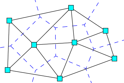
Figure 7: Dual relationship between Voronoi diagram and Delaunay Triangulation.

A DT is a planar subdivision of $\mathbb{R}^{k}$, constructed by drawing edges connecting any two cell sites that share an edge between their VD cells, and as a result, the closest pair of sites in a VD is represented as neighbors in the DT. In this way, each cell in the VD corresponds to a vertex in the dual complex. Figure 7 illustrates this primal dual relationship. We have explored representing a new feature vector as a weighted combination of the features that define the DT simplex in which it falls in place of our $k$-$d$ tree representation in Phase III.

An important and non-trival consideration that must be taken into account for representing a manifold is the time complexity required to construct the data structure used to represent it. While we have found the DT approach to produce approximately comparable results to those produced by the proposed $k$-$d$ tree method on the COMPAS dataset, the time complexity for computing a DT from $N$ feature vectors in dimension $k$ is $\mathcal{O}(N^{\lceil k\rceil})$. On the other hand, the time complexity of constructing a $k$-$d$ tree is $\mathcal{O}(kNlog(N))$, which is far less expensive. To illustrate this disparity, we present the time complexities in seconds associated with computing these data structures for Groups 1 and 2 for the COMPAS and Law datasets in Table IV. A clear and stark contrast between the costs associated with computing DTs and $k$-$d$ trees can clearly be observed in this table. In particular, the $k$-$d$ tree is always able to be computed in milliseconds for each group in both datasets. Conversely, no DT is able to be constructed in a relatively similar amount of time. Notable, for the Law dataset, group’s associated DT is able to be computed in under 12 hours even though the number of samples in Group 2 of both the COMPAS and Law datasets are similar. This emphasizes the scalability issues associated with using the DT for manifold representation in higher dimensions.

TABLE IV: Time complexity comparison for constructing data structures. Results are presented in seconds across five trials. Processes not terminated within 12 hours reported as "—."

	Compas		Law
	Group 1	Group 2	Group 1	Group 2
DT	$172.59_{\pm 1.73}$	$905.46_{\pm 21.876}$	—	—
$k$-$d$ tree	$0.001_{\pm 0.000}$	$0.001_{\pm 0.000}$	$0.008_{\pm 0.000}$	$0.002_{\pm 0.001}$

VI-B Limitations and Mitigations

For the proposed algorithm to work well in achieving both inter- and within-group fairness, the following assumption must approximately hold: if the distance between the scores of two feature vectors is close, then the distance between these feature vectors in the input space should be close. This assumption holds well on for the COMPAS and Law datasets, but may not hold in general. If this situation fails, feature vectors that are close in the group domain may map to feature vectors that are far from each other in the population domain. Thus, and convex sum of these population feature vectors may lie outside the population manifold. To resolve this issue in our on-going research, we are investigating new approaches for constructing feature correspondences between the group and population manifolds.

Note that the mapping constructed in the configuration of the pre-processing framework proposed in this paper requires storing the entire training dataset in the $k$-$d$ tree data structure. While this approach allowed us to construct an interpretable mapping mapping between a group and the population manifold, more compact representations may potentially be constructed by incorporating the mapping constructing into the learning process. We plan to further investigate such solutions in our future work.

We would lastly like to observe that the focus of this work has been analyzing the effectiveness of our framework on tabular data. Nevertheless, our framework has the potential to be generalized to other forms of data, such as image data. While such data in its raw form may exist in much higher dimensions, which may produce a computational burden when constructing the $k$-$d$ tree, our framework may be applied to the features in the latent space of intermediate layers in an ML model or on feature vectors to which dimensionality reduction has first be applied.

VII Conclusion

In this paper, we study the importance of maintaining within-group fairness in situations where inter-group fairness is required. We introduce a notion of within-group fairness and a tool for measuring it. We have adopted the stricter threshold invariant form of demographic parity for analyzing inter-group fairness, which requires the scores generated for different groups to be equally distributed. Furthermore, we provide a pre-processing framework to map raw features to a canonical domain before applying a classifier and it is able to achieve high levels of inter-group and within-group fairness. This new framework requires that the sensitive group attributes are used only in a pre-processing stage to transform raw features to a canonical domain in the testing stage of the machine learning process, and these attributes are never explicitly used by the classifier to make decisions. To verify its effectiveness, we compare the performance of our framework to models in which fairness is embedded in the training process through regularization. Experimental results demonstrate that our pre-processing framework can achieve both inter-group and within-group fairness with little penalty on accuracy.

Appendix A Appendix

In this section, we provide details on the meaning of each of the features used for classification in COMPAS [25] and Law [31] datasets. These descriptions are respectively provided in Tables  V and  VI.

TABLE V: Feature descriptions for the COMPAS dataset

Feature	Description
age	age of the defendant
sex	sex of the defendant
juv_fel_count	# of felonies committed by defendant as a juvenile
juv_misd_count	# of misdemeanors committed by defendant as a juvenile
juv_other_count	# of other crimes committed by defendant as a juvenile
priors_count	# of prior criminal records of defendants
c_charge_degree	Charge degree of defendant (felony or misdemeanor)

TABLE VI: Feature descriptions for the Law dataset

Feature	Description
decile1b	Decile in the school given student’s grades in Year 1
decile3	Decile in the school given student’s grades in Year 3
lsat	LSAT score
ugpa	Undergraduate GPA
zfygpa	First year law school GPA
zgpa	Cumulative law school GPA
fulltime	Whether the student will work full-time or part-time
family income	Student’s family income bracket
sex	Student’s sex
tier	Student’s Tier

References

- [1] FDIC Consumer Compliance Examination Manual, 2021.
- [2] Adewole S Adamson and Avery Smith. Machine learning and health care disparities in dermatology. JAMA Dermatology, 154(11):1247–1248, 2018.
- [3] Dongsheng An, Yang Guo, Na Lei, Zhongxuan Luo, Shing-Tung Yau, and Xianfeng Gu. Ae-Ot: A new generative model based on extended semi-discrete optimal transport. International Conference on Learning Representations, 2020.
- [4] Julia Angwin, Jeff Larson, Surya Mattu, and Lauren Kirchner. Machine bias. In Ethics of Data and Analytics, pages 254–264. Auerbach Publications, 2016.
- [5] Toon Calders and Sicco Verwer. Three naive bayes approaches for discrimination-free classification. Data Mining and Knowledge Discovery, 21(2):277–292, 2010.
- [6] Jiahao Chen, Nathan Kallus, Xiaojie Mao, Geoffry Svacha, and Madeleine Udell. Fairness under unawareness: Assessing disparity when protected class is unobserved. In Proceedings of the Conference on Fairness, Accountability, and Transparency, pages 339–348, 2019.
- [7] Mingliang Chen and Min Wu. Towards threshold invariant fair classification. In Conference on Uncertainty in Artificial Intelligence, pages 560–569. PMLR, 2020.
- [8] Alexandra Chouldechova. Fair prediction with disparate impact: A study of bias in recidivism prediction instruments. Big Data, 5(2):153–163, 2017.
- [9] Jeffrey Dastin. Amazon scraps secret AI recruiting tool that showed bias against women. In Ethics of Data and Analytics, pages 296–299. Auerbach Publications, 2018.
- [10] Mark Theodoor De Berg, Marc Van Kreveld, Mark Overmars, and Otfried Schwarzkopf. Computational Geometry: Algorithms and Applications. Springer Science & Business Media, 2000.
- [11] Cynthia Dwork, Moritz Hardt, Toniann Pitassi, Omer Reingold, and Richard Zemel. Fairness through awareness. In Proceedings of the 3rd Innovations in Theoretical Computer Science Conference, pages 214–226, 2012.
- [12] Michael Feldman, Sorelle A Friedler, John Moeller, Carlos Scheidegger, and Suresh Venkatasubramanian. Certifying and removing disparate impact. In Proceedings of the 21th ACM SIGKDD International Conference on Knowledge Discovery and Data Mining, pages 259–268, 2015.
- [13] Sorelle A Friedler, Carlos Scheidegger, and Suresh Venkatasubramanian. On the (im) possibility of fairness. arXiv preprint arXiv:1609.07236, 2016.
- [14] Rafael C. González and Richard E. Woods. Digital Image Processing, 3rd Edition. Pearson Education, 2008.
- [15] Moritz Hardt, Eric Price, and Nati Srebro. Equality of opportunity in supervised learning. Advances in Neural Information Processing Systems, 29, 2016.
- [16] Le Hou, Chen-Ping Yu, and Dimitris Samaras. Squared earth mover’s distance-based loss for training deep neural networks. arXiv preprint arXiv:1611.05916, 2016.
- [17] Christina Ilvento. Metric learning for individual fairness. In 1st Symposium on Foundations of Responsible Computing, 2020.
- [18] Matthew Joseph, Michael Kearns, Jamie H Morgenstern, and Aaron Roth. Fairness in learning: Classic and contextual bandits. Advances in Neural Information Processing Systems, 29, 2016.
- [19] Christopher Jung, Michael J Kearns, Seth Neel, Aaron Roth, Logan Stapleton, and Zhiwei Steven Wu. Eliciting and enforcing subjective individual fairness. CoRR, 2019.
- [20] Faisal Kamiran and Toon Calders. Data preprocessing techniques for classification without discrimination. Knowledge and Information Systems, 33(1):1–33, 2012.
- [21] Toshihiro Kamishima, Shotaro Akaho, Hideki Asoh, and Jun Sakuma. Fairness-aware classifier with prejudice remover regularizer. In Joint European Conference on Machine Learning and Knowledge Discovery in Databases, pages 35–50. Springer, 2012.
- [22] Michael Kearns, Seth Neel, Aaron Roth, and Zhiwei Steven Wu. Preventing fairness gerrymandering: Auditing and learning for subgroup fairness. In International Conference on Machine Learning, pages 2564–2572. PMLR, 2018.
- [23] Jon Kleinberg, Sendhil Mullainathan, and Manish Raghavan. Inherent trade-offs in the fair determination of risk scores. 09 2016.
- [24] Matt J Kusner, Joshua Loftus, Chris Russell, and Ricardo Silva. Counterfactual fairness. Advances in Neural Information Processing Systems, 30, 2017.
- [25] Jeff Larson, Surya Mattu, Lauren Kirchner, and Julia Angwin. How we analyzed the COMPAS recidivism algorithm. ProPublica (5 2016), 9(1):3–3, 2016.
- [26] Ninareh Mehrabi, Umang Gupta, Fred Morstatter, Greg Ver Steeg, and Aram Galstyan. Attributing Fair Decisions with Attention Interventions. arXiv preprint arXiv:2109.03952, 2021.
- [27] Ninareh Mehrabi, Fred Morstatter, Nripsuta Saxena, Kristina Lerman, and Aram Galstyan. A survey on bias and fairness in machine learning. ACM Computing Surveys (CSUR), 54(6):1–35, 2021.
- [28] Elhanan Mishraky, Aviv Ben Arie, Yair Horesh, and Shir Meir Lador. Bias detection by using name disparity tables across protected groups. Journal of Responsible Technology, 9:100020, 2022.
- [29] Debarghya Mukherjee, Mikhail Yurochkin, Moulinath Banerjee, and Yuekai Sun. Two simple ways to learn individual fairness metrics from data. In International Conference on Machine Learning, pages 7097–7107. PMLR, 2020.
- [30] Latanya Sweeney. Discrimination in online ad delivery. Communications of the ACM, 56(5):44–54, 2013.
- [31] Linda F Wightman. LSAC national longitudinal bar passage study. LSAC research report series. 1998.
- [32] Muhammad Bilal Zafar, Isabel Valera, Manuel Gomez Rodriguez, and Krishna P Gummadi. Fairness beyond disparate treatment & disparate impact: Learning classification without disparate mistreatment. In Proceedings of the 26th international conference on world wide web, pages 1171–1180, 2017.
- [33] Muhammad Bilal Zafar, Isabel Valera, Manuel Gomez Rogriguez, and Krishna P Gummadi. Fairness constraints: Mechanisms for fair classification. In Artificial intelligence and statistics, pages 962–970. PMLR, 2017.
- [34] Rich Zemel, Yu Wu, Kevin Swersky, Toni Pitassi, and Cynthia Dwork. Learning fair representations. In International Conference on Machine Learning, pages 325–333. PMLR, 2013.
- [35] Han Zhao and Geoffrey J Gordon. Inherent tradeoffs in learning fair representations. The Journal of Machine Learning Research, 23(1):2527–2552, 2022.