Electromagnetic Properties of Indium Isotopes Elucidate the Doubly Magic Character of ¹⁰⁰Sn

Abstract

Our understanding of nuclear properties in the vicinity of ¹⁰⁰Sn, suggested to be the heaviest doubly magic nucleus with equal numbers of protons ($\mathbf{\textit{Z}=50}$) and neutrons ($\mathbf{\textit{N}=50}$), has been a long-standing challenge for experimental and theoretical nuclear physics. Contradictory experimental evidence exists on the role of nuclear collectivity in this region of the nuclear chart. Using precision laser spectroscopy, we measured the ground-state electromagnetic moments of indium ($\mathbf{\textit{Z}=49}$) isotopes approaching the $\mathbf{\textit{N}=50}$ neutron number down to ¹⁰¹In, and nuclear charge radii of ^101-131In spanning almost the complete range between the two major neutron closed-shells at $\mathbf{\textit{N}=50}$ and $\mathbf{\textit{N}=82}$. Our results for both nuclear charge radii and quadrupole moments reveal striking parabolic trends as a function of the neutron number, with a clear reduction toward these two neutron closed-shells, thus supporting a doubly magic character of ¹⁰⁰Sn. Two complementary nuclear many-body frameworks, density functional theory and ab initio methods, elucidate our findings. A detailed comparison with our experimental results exposes deficiencies of nuclear models, establishing a benchmark for future theoretical developments.

I.0  Introduction

Studying magic nuclei has guided our understanding of atomic nuclei. In analogy with the filled electron shells in atomic noble gasses, these nuclear systems with filled proton or neutron shells exhibit relatively simple structures with enhanced binding and high energies of excited states ^{1, 2, 3}. The area of the nuclear chart surrounding the $N=Z=50$ isotope ¹⁰⁰Sn is of particular interest as this isotope has been proposed to be doubly magic with closed shells of protons and neutrons ^{4, 5}.

The importance of nuclear structure studies approaching ¹⁰⁰Sn has been widely recognized ^{6, 4, 7, 8, 9, 10, 11, 12, 13, 14, 15, 16, 17}. Theoretically, significant progress has been achieved in describing isotopes around ¹⁰⁰Sn. Complementary many-body methods can now calculate ground state properties (binding energies, radii, and electromagnetic moments) of these nuclei^{3, 13, 14, 18, 19, 16, 20}. However, despite great interest, the experimental knowledge of this neutron-deficient region of the nuclear chart is still incomplete due to low production yields. In particular, contradictory experimental evidence exists on the evolution of collective properties when approaching ¹⁰⁰Sn ^{7, 4, 10, 21, 22} (see Fig. 2a).

Here, we report results on the hyperfine structure and isotope shifts from precision laser spectroscopy experiments performed on neutron-deficient indium ($Z=49$) isotopes down to the neutron number $N=52$ and neutron-rich indium isotopes up to $N=82$. These data allowed us to extract the nuclear quadrupole moments, magnetic dipole moments, and charge radii. This makes it possible to comprehensively describe the evolution of nuclear structure towards the $N=50$ closed shell. With a single proton hole in the $Z=50$ shell, the electromagnetic properties of indium isotopes provide a compelling laboratory to study the interplay between single-particle and collective properties of nuclei between the two major neutron-closed shells $N=50$ and $N=82$. The study of indium isotopes dates back almost 100 years, where investigations of its stable isotopes provided some of the earliest indications of nuclear deformation ²³.

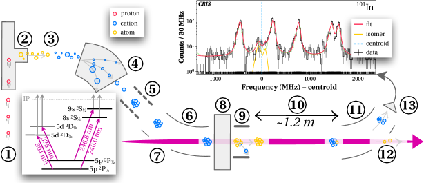
Figure 1: Schematic of the CRIS experiment at CERN-ISOLDE: (1) 1.4 GeV protons from CERN’s Proton Synchrotron Booster, (2) nuclear reactions inside a lanthanum carbide target at the ISOLDE facility, (3) resonant laser ionization with RILIS, (4) magnetic mass selection, (5) bunching and cooling in ISCOOL, (6) bending into the CRIS beamline, (7) laser port, (8) charge-exchange cell, (9) deflection of ions, (10) laser-interaction area ($\sim$1.2 m), (11) bending of resonantly ionized particles of interest, (12) laser port and beam dump for contaminants (not ionized), (13) particle detector for resonantly ionized particles of interest. The plot at the top right shows part of an example spectrum for the $I^{\pi}=9/2^{+}$ ground state and $I^{\pi}=1/2^{-}$ isomer in ¹⁰¹In with a fitted theoretical line shape (red line; 30 MHz binning). The inset at the bottom left shows the first resonant laser excitation transitions used for the ionization at RILIS (left two) and spectroscopy (right two). See text for details. A color version of the article can be found online.

II.0  Experimental and Theoretical Developments

The ^101-131In isotopes were produced in two separate campaigns at the Isotope Separator On-Line Device (ISOLDE) at CERN, where a 1.4 GeV proton beam from CERN’s Proton Synchrotron Booster induces nuclear reactions in thick lanthanum (in the case of ^101-115In) or uranium (in the case of ^113-131In; see also Ref. ²⁰) carbide targets, with the latter one employing a proton-to-neutron converter ²⁴ to suppress isobaric contamination. These reactions produce a multitude of short-lived isotopes of different chemical elements. Through diffusion by heating the target to $>2000\,^{\circ}$C, these nuclides are extracted from the target and subsequently ionized via multi-step, element-selective, resonant laser ionization ²⁵ (see 304 nm and 325 nm laser transitions in Fig. 1). The ions are then accelerated to 39948(1) eV (in the case of ^101-115In) or $40034(1)\,$eV²⁰ (in the case of ^113-131In) and mass-selected for the isotope of interest using ISOLDE’s separator magnets.

Following cooling and bunching in ISOLDE’s radio-frequency quadrupole trap ²⁶, the ions are guided into the Collinear Resonance Ionization Spectroscopy (CRIS) setup ²⁷. At CRIS, the arriving ion bunch is neutralized through electron exchange with sodium vapor to be left with a fast neutral beam ²⁸. This atom beam is overlapped with lasers both temporally and spatially to induce a multi-step ionization and finally deflected onto an ion detector, resulting in nearly background-free signal detection. The Methods section in Ref.²⁰ gives more details on the setup.

The hyperfine spectrum is measured by scanning the first laser step over the 246.0 nm and 246.8 nm transitions (see the two right magenta laser transitions and the resulting ¹⁰¹In spectrum in Fig. 1). Magnetic dipole and electric quadrupole parameters, $A_{\text{hf}}$ and $B_{\text{hf}}$, as well as isotope shifts of the $I^{\pi}=9/2^{+}$ nuclear ground state and the $I^{\pi}=1/2^{-}$ nuclear-excited state (if applicable), were extracted from the measured spectra (see Methods-A for details).

The results are presented in Tables 1 and 2. Tab. 1 lists the spectroscopic nuclear quadrupole moments $Q_{\rm{s}}$ and Tab. 2 presents the differential mean-square nuclear charge radii $\updelta\langle r^{2}\rangle$. The nuclear magnetic moments $\mu$ presented in Tab. 1 are calculated following the description in Ref. ²⁰, continue the trend from the same article, and agree with our density functional theory (DFT) results.

The data collection is described in Ref. ²⁰. Details of the data analysis for the ^101-115In isotopes can be found in the Methods section B, and for the ^117-131In isotopes in Ref. ²⁰.

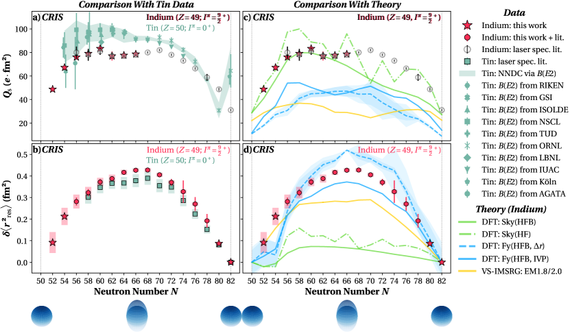
Figure 2: Evolution of the nuclear deformation between the two magic neutron numbers $N=50$ and 82 from measurements in even-$N$, ground-state indium isotopes ($Z=49$; black circles = literature; red stars = this work; $I^{\pi}$=9/2⁺) in comparison to measurements in even-$N$, ground-state tin isotopes ($Z=50$; mint = literature; $I^{\pi}$=0⁺) in the left column, and to nuclear theory (colored lines) in the right column. The blue spheres at the bottom represent a visual guide for the evolution of nuclear deformation between the two closed shells at $N=50$ and 82. A color version of the article can be found online.
  –  a/c) Spectroscopic quadrupole moments $Q_{\rm{s}}$ with their experimental uncertainties. Indium: Laser spectroscopy results from this work (red stars; 5p ²P${}_{\nicefrac{{3}}{{2}}}\,$→ 9s ²S${}_{\nicefrac{{1}}{{2}}}$ transition) and literature (black circles; Ref. ²⁰ for $N>74$ (same transition) and Ref. ²⁹ for $54<N<74$ (different 5p ²P${}_{\nicefrac{{3}}{{2}}}\,$→ 6s ²S${}_{\nicefrac{{1}}{{2}}}$ transition and recalculated based on the latest atomic theory published in Ref. ³⁰)) with their experimental uncertainties; Tin: Numerous $B(E2)$ measurements (mint borderless markers) converted to spectroscopic quadrupole moments $Q_{\rm{s}}$ using Eq. 6 in ¹⁵ from RIKEN ³¹, GSI ^{32, 33, 34, 9}, ISOLDE ^{35, 36}, MSU ^{37, 8}, TUD ¹⁴, ORNL ^{38, 39, 40, 41}, LBNL ⁴², IUAC ⁴³, Köln ¹⁴, GANIL ⁴⁴ and shown with their 2016 average by NNDC ⁴⁵ as a mint one-sigma uncertainty band. Theory: Selected density-functional and ab initio calculations. For details, see the text.
  –  b/d) Residual differential charge radii $\updelta\langle r^{2}_{\rm{res}}\rangle$ with their experimental (thin) and theory-derived (broad) uncertainties. Indium: Laser spectroscopy results as a weighted average of both transitions from this work (red stars) and including the two recalculated transitions from Ref. ²⁹ (red circles), if available, (for details, see Methods-F). Tin: Laser spectroscopy results from literature ³ in mint square markers. Theory: Selected density-functional and ab initio calculations. For details, see the text and Methods-E and F.

Our experimental results are compared with predictions from two complementary many-body methods, the valence-space formulation of the ab initio in-medium-similarity-renormalization-group (VS-IMSRG) and nuclear DFT. The VS-IMSRG calculations ^{46, 47} (see Methods-G for further details) were performed using two- and three-nucleon interactions derived from chiral effective field theory ^{48, 49} and are labeled “1.8/2.0(EM)” ⁵⁰ and “$\Delta$N²LO_GO” ⁵¹. The former is constrained by properties of two-, three- and four-nucleon systems and reproduces ground-state energies across the nuclear chart while underpredicting absolute charge radii ^{13, 52}. $\Delta$N²LO_GO was recently developed to include $\Delta$-isobar degrees of freedom and is also fit to reproduce saturation properties of infinite nuclear matter, thereby improving radii predictions. Converged values for all observables discussed here were obtained with a novel storage scheme allowing sufficiently large inclusion of three-nucleon force matrix elements ⁵³. Both interactions produce similar results for $Q_{\rm{s}}$ and $\updelta\langle r^{2}\rangle$; hence only the 1.8/2.0(EM) results are presented.

We performed DFT calculations for neutrons using the Hartree–Fock (HF; labeled ”DFT: Sky(HF)”) and Hartree–Fock–Bogoliubov (HFB; labeled ”DFT: Sky(HFB)”) approaches, i.e., single-nucleon (HF) or nucleon–hole pair excitations (HFB) as basis states with HFB introducing some pairing correlations. For protons, the HF single-hole configuration was used. Calculations were performed for the UNEDF1 Skyrme functional ⁵⁴ using the methodology recently developed in Ref.^{55, 56}.

We also considered other energy density functionals: a Skyrme functional SV-min ⁵⁷ with mixed volume and surface pairing at BCS level ⁵⁸, Fy(HFB, $\Delta r$) ⁵⁹ a Fayans functional with additional gradient terms in surface energy and pairing ⁶⁰ employing full HFB, and Fy(HFB, IVP) as a Fayans functional in which proton- and neutron-pairing terms have different strengths (for details, see Methods-H). All three parametrizations are fitted to the same pool of ground-state properties from Ref. ⁵⁷. At the same time, the two Fayans functionals include differential radii in the calibration dataset to reproduce the isotopic trends of charge radii better. In all cases, odd-even isotopes were computed by blocking the proton $K=9/2^{+}$ orbital. The statistical uncertainties stemming from parameter calibration were estimated using linear regression ⁶¹. To simplify the presentation, we show the uncertainties only for Fy(HFB, $\Delta r$). The uncertainty bands for the other two cases are comparable. The SV-min approach and UNEDF1 Skyrme functionals, without a full treatment of pairing, give comparable results. Hence, only ”DFT: Sky(HF)” and ”DFT: Sky(HFB)” calculations with UNEDF1 are shown in the figures for clarity. Both DFT and ab initio calculations were carried out with bare nucleon charges.

III.0  Results and Discussion

Collective properties of nuclei around ¹⁰⁰Sn have been the focus of intense interest in nuclear physics laboratories worldwide. As the ground states of even-even tin isotopes have nuclear spin $I\,=\,0$, the evolution of their quadrupole collectivity can be studied by measuring the $B(E2)$ rate for exciting their first $2^{+}$ states. The experimental results for the tin isotopic chain are summarized in Fig. 2a) after conversion to spectroscopic quadrupole moments $Q_{\rm{s}}$ ¹⁵ to enable direct comparison with the spectroscopic quadrupole moments of indium.

Similar to the nuclear quadrupole moments of indium²⁰, a reduction of the $B(E2)$ values in tin towards $N=82$ indicates a reduction in collectivity ⁴⁴, thus providing evidence for the doubly magic character of ¹³²Sn($Z=50,N=82$). However, the large uncertainties of $B(E2)$ values for neutron-deficient tin isotopes do not allow an unambiguous conclusion toward $N=50$. See also results of recent lifetime measurements in odd-$N$ systems in the region ⁶². Our new high-precision $Q_{\rm{s}}$ results in indium establish a clear reduction in collective properties towards $N=50$ for the first time, thus strongly supporting the doubly magic character of ¹⁰⁰Sn($Z=N=50$). In fact, the indium $Q_{\rm{s}}$ at $N=50+2$ and $N=82-2$ agree well within one combined standard deviation, thereby suggesting a similar proton and a vanishing neutron core polarization at $N=50$ and $N=82$ ²⁰, the $E2$-level signature of a doubly magic shell closure^{63, 64}.

While differential charge radii $\updelta\langle r^{2}\rangle$ generally increase on average with increasing neutron number, an additional small parabolic trend found between shell closures also provides sensitivity to nuclear deformation^{3, 65, 66}. This parabolic trend can be emphasized by subtracting the overall linear reference. The resulting ”residual” differences $\updelta\langle r^{2}_{\rm{res}}\rangle$, shown in Fig. 2b), were obtained by fitting the experimental data set with a parabolic function and removing the linear trend between the fit’s values at $N=50$ and $N=82$ (see also Methods-E and F for details).

In both indium and tin, the reduction in residual differential radii $\updelta\langle r^{2}_{\rm{res}}\rangle$ towards $N=82$ indicates a decrease in collectivity, thus providing evidence for the established doubly magic character of ¹³²Sn($Z=50,N=82$)³. However, while the extent of existing precision tin radii (limited to $N\geq 58$³) and indium radii (limited to $N\geq 56$²⁹) prevented a conclusion toward $N=50$, our new high-precision results for $\updelta\langle r^{2}_{\rm{res}}\rangle$ in indium down to ¹⁰¹In($N=52$) present a clear reduction towards $N=50$ for the first time. Well-aligned with our conclusions for $Q_{\rm{s}}$, this reduction in $\updelta\langle r^{2}_{\rm{res}}\rangle$ also strongly supports the doubly magic character of ¹⁰⁰Sn($Z=N=50$).

The experimental results are compared with the theoretical predictions in Fig. 2c) for quadrupole moments, and Fig. 2d) for residual differential charge radii. Both the DFT and VS-IMSRG calculations predict parabolic trends for the quadrupole moments. However, the magnitude of $Q_{\rm{s}}$ is significantly underestimated by the VS-IMSRG calculations. This underestimation is observed in all ab initio calculations based on spherical references and results from neglected many-particle, many-hole excitations when truncated at the two- or three-body levels⁶⁷. We note, however, that quadrupole collectivity is well reproduced by methods based on deformed references⁶⁸. The difference in the DFT predictions for quadrupole moments is closely related to pairing strength differences. While Skyrme-functional-based calculations without a full treatment of pairing reproduce the $Q_{\rm{s}}$ trend well, the Fayans with a full (”Fy(HFB, $\Delta r$)”) and enhanced (”Fy(HFB, IVP)”) pairing strength show a clear decrease in quadrupole moments with increasing pairing strength. This decrease in $Q_{\rm{s}}$ results from pairing driving the nucleus towards a spherical shape against the increase of other deformation effects at the mid-shell ⁶⁹. Thus, in contrast to the charge radii results discussed next, adding a full treatment of pairing does not improve the agreement with experiment.

All theories generally reproduce the dominating linear trend in the differential charge radii (a plot of the trend can be found, for completion, in Methods-E). However, the parabolic behavior (Fig. 2d) between the closed shells is reproduced by the VS-IMSRG results (although somewhat underestimated), while only the DFT-Fayans calculations with a full treatment of pairing closely approach the observed trend. DFT-Skyrme-based calculations without full pairing underestimate the curvature.

In conclusion, both the radii and quadrupole moments indicate that quadrupole deformation dominates the ground states in the indium isotopes in the neutron mid-shell region, similar to what has been indicated for Sn isotopes ¹⁵. However, the inverse DFT behavior between $Q_{\rm{s}}$ and $\updelta\langle r^{2}_{\rm{res}}\rangle$ in the prediction of nuclear deformation with an increase in pairing strength highlights missing nucleus-deforming effects (e.g., quadrupole vibrations) in state-of-the-art DFT functionals. Extensive correlation studies between $Q_{\rm{s}}$ and $\updelta\langle r^{2}\rangle$ for different DFT parametrizations, described in more detail in Methods-I, confirm this conclusion. Meanwhile, the use of nucleon-hole pair excitations (HFB) over single-nucleon (HF) basis states in DFT, recently found to be crucial in describing nuclear magnetic moments when approaching a shell closure ²⁰, seems to have a negligible effect on both $Q_{\rm{s}}$ and $\updelta\langle r^{2}_{\rm{res}}\rangle$ (green lines in Figs. 2c) and d).

Table 1: Magnetic dipole and electric quadrupole hyperfine parameters, $A_{\rm{hf}}$ and $B_{\rm{hf}}$, spectroscopic nuclear quadrupole moments $Q_{\rm{s}}$ (using the calculated electric-field gradient $\updelta^{2}V/\updelta z^{2}=57,600(400)\,e\cdot$fm²/MHz) from Ref. ³⁰), and nuclear magnetic moments (see Methods-B for details) for $I^{\pi}=9/2^{+}$ ground states and $I^{\pi}=1/2^{-}$ excited states (if available) of odd-$A$ indium ($Z=49$) isotopes using 246.0 nm (5p ²P${}_{\nicefrac{{1}}{{2}}}\,$→ 8s ²S${}_{\nicefrac{{1}}{{2}}}$) and 246.8 nm (5p ²P${}_{\nicefrac{{3}}{{2}}}\,$→ 9s ²S${}_{\nicefrac{{1}}{{2}}}$) transitions. The results are compared to literature values²⁹ in italic font measured with the 451 nm (5p ²P${}_{\nicefrac{{3}}{{2}}}\,$→ 6s ²S${}_{\nicefrac{{1}}{{2}}}$) transition. Experimental uncertainties are in parenthesis, and theory-derived ones are in brackets.

Table 2: Isotope shifts (IS) and resulting differential mean square nuclear charge radii $\updelta\langle r^{2}\rangle$ with respect to the centroid of the stable ¹¹⁵In for $I^{\pi}=9/2^{+}$ ground states of odd-$A$ indium ($Z=49$) isotopes for the 246.0 nm (5p ²P${}_{\nicefrac{{1}}{{2}}}\,$→ 8s ²S${}_{\nicefrac{{1}}{{2}}}$) and 246.8 nm (5p ²P${}_{\nicefrac{{3}}{{2}}}\,$→ 9s ²S${}_{\nicefrac{{1}}{{2}}}$) transitions (using the calculated field and mass shifts from Ref. ⁷⁰, and the atomic mass values from Ref. ⁷¹). Our results are compared to literature values²⁹ in italic font measured with the 451 nm (5p ²P${}_{\nicefrac{{3}}{{2}}}\,$→ 6s ²S${}_{\nicefrac{{1}}{{2}}}$) transition. Experimental uncertainties are in parenthesis, and theory-derived ones are in brackets.

IV.0  Outlook

Compelling evidence for the doubly magic character of ¹⁰⁰Sn ($Z=N=50$) has been provided by the first precision determination of the nuclear quadrupole moments and differential charge radii of neutron-deficient indium ($Z=49$) isotopes down to ¹⁰¹In. Just one proton below tin ($Z=50$), the examined odd-$A$ ^101-131In nuclei have provided key insights into the evolution of collective nuclear properties towards the neutron number $N=50$ around $Z=50$. The extracted parabolic trends exhibit a clear reduction toward the neutron numbers $N=50$ and $N=82$, in agreement with a reduction of collective properties expected at magic neutron numbers.

State-of-the-art ab initio and density-functional calculations describe the experimental findings well. Although these calculations describe the overall experimental trends, they fall short of capturing the local variations of the nuclear quadrupole moments and charge radii trends. Including many-body correlations sufficient to fully capture quadrupole collectivity remains a challenge for ab initio approaches based on spherical references, such as the VS-IMSRG presented here. Our findings also highlight missing effects to capture nuclear deformation in the latest density functionals of great importance in guiding these theoretical developments.

Efforts to produce even more exotic neutron-deficient tin and indium isotopes are ongoing at ISOLDE. Moreover, the next-generation RIB facilities now in operation, such as FRIB in the U.S., RIKEN in Japan, and SPIRAL2 in France, will enable the study of ¹⁰⁰Sn and its immediate neighbors.

Methods

Appendix A Hyperfine Spectrum from Raw Data

The raw time-of-flight information per resonantly ionized ion was recorded on a MagneTOF™detector by ETP Electron Multipliers Pty. Ltd. and correlated with a Doppler-shift corrected wavemeter readout of the scanning laser frequency (see the right two magenta transitions in Fig. 1) in the rest frame of the ion at $V_{0}=39948(1)\,$eV (in the case of ^101-115In) or $40034(1)\,$eV²⁰ (in the case of ^113-131In). The time-of-flight distribution was used to remove isobaric contamination and trigger noise from the ion signal at its mass-dependent time of flight $t_{i}=\sqrt{\frac{2eV_{0}}{m_{i}}}$ with the elementary charge $e$. The pure hyperfine spectrum was then plotted as counts per frequency bin at the 5 MHz minimal resolution limited by the wavemeter. While the minimal bin width was typically used for fitting the spectra, studies using different bin widths up to 50 MHz were performed and used as the basis for the systematic fit uncertainty.

Appendix B Hyperfine Parameter and Centroid Frequencies

This section focuses on the analysis of ^101-115In. Details on the ^117-131In isotopes can be found in Ref. ²⁰.

The hyperfine parameters, $A_{\rm{hf}}$ and $B_{\rm{hf}}$, as well as the centroid frequency, $\nu_{0}$, were determined through Bayesian analysis by use of binned maximum likelihood estimation. An independent analysis using the SATLAS package ⁷² was used to confirm the validity of the new code.

Due to the complex nature of the cumulative distribution function of the Voigt profile required for binned maximum likelihood estimation, the peak shape was estimated with a pseudo-Voigt profile using the parameters published in Ref. ⁷³. Extensive Monte-Carlo studies were performed to verify the validity of this approximation, and deviations were found to be well within one standard deviation of the statistical uncertainty of the fit.

From all 80+ individual measurements of isotopes ranging from ^101-115In, the weighted average was calculated for the hyperfine parameters per individual isotope and transition (labeled “i”). From this data, the magnetic moments $\mu_{\rm{i}}=\frac{I_{\rm{i}}}{I_{\rm{ref}}}\cdot\frac{A_{\rm{hf},i}}{A_{\rm{hf,ref}}}\cdot\mu_{\rm{ref}}$ and quadrupole moments $Q_{\rm{i}}=\frac{B_{\rm{hf},i}}{e\cdot\delta^{2}V/\delta z^{2}}$ were calculated using the nuclear spin $I$ and the nuclear $E$-field gradient $\updelta^{2}V/\updelta z^{2}=57,600(400)\,e\cdot$fm²/MHz ³⁰. In our case, the weighted average for the stable and highly abundant ¹¹⁵In was used as a reference isotope (labeled “ref”) to minimize systematic uncertainties from our measurement. In the case of the magnetic moments, the weighted average with the weighted standard deviation as its uncertainty of the four resulting values per isotope from the two studied transitions was calculated using $\mu_{\rm{ref}}=5.5408(2)\mu_{N}$ ⁷⁴. All values are presented in Tab. 1.

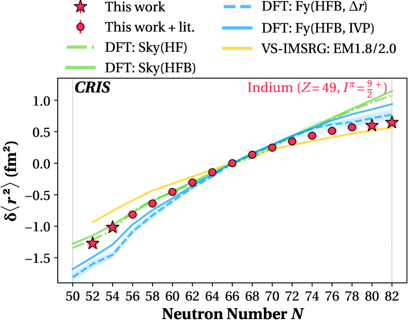
Figure 3: Differential charge radii $\updelta\langle r^{2}\rangle$ of odd indium $I^{\pi}=9/2^{+}$ ground states with respect to the charge radius of ¹¹⁵In⁷⁵ as a weighted average of both transitions from this work (red stars) and including the two recalculated transitions from Ref. ²⁹ (red circles), if available, (for details, see Methods-F) with experimental (thin) and theory-derived (thick) uncertainties compared to theoretical calculations (colored lines). A color version of the article can be found online.

Appendix C Atomic Calculations

The differential charge radii $\updelta\langle r^{2}\rangle=\frac{\nu_{i}-\nu_{\rm{ref}}}{F}-\frac{M}{F}\cdot\frac{A_{i}-A_{\rm{ref}}}{A_{i}\cdot A_{\rm{ref}}}$ were calculated from the isotope shift $\Delta\nu_{i}=\nu_{i}-\nu_{\rm{ref}}$, the mass numbers $A$ with $A_{\rm{ref}}=115$, the mass shift constant $M=(K_{SMS}+K_{NMS})$ and the field shift constant $F$. We have improved calculations of isotope shift constants over our previous results ⁷⁶ by considering single, double, and triple excitation approximations in the analytical response coupled-cluster (AR-RCC) theory. In addition, we have included atomic orbitals belonging up to orbital angular momentum $l=6$ in contrast to our previous work where orbitals up to $l=4$ value were only considered. Corrections from the Breit and lower-order quantum electrodynamics interactions are also accounted for, improving the accuracy of the calculations. Detailed discussions on these improvements can be found in Ref. ⁷⁰. As a result, we have obtained $M=325(71)\,$GHz/u and $F=1.577(15)\,$GHz for the 5p²P${}_{\nicefrac{{3}}{{2}}}$→9s²S${}_{\nicefrac{{1}}{{2}}}$ transition, $M=216(51)\,$GHz/nucleon and $F=1.626(15)\,$GHz for the 5p²P${}_{\nicefrac{{1}}{{2}}}$→8s²S${}_{\nicefrac{{1}}{{2}}}$ transition, $M=-92(74)\,$GHz/nucleon and $F=1.889(16)\,$GHz for the 5p²P${}_{\nicefrac{{3}}{{2}}}$→6s²S${}_{\nicefrac{{1}}{{2}}}$ transition from Ref. ²⁹, and $M=-158(55)\,$GHz/nucleon and $F=1.913(16)\,$GHz for the 5p²P${}_{\nicefrac{{1}}{{2}}}$→6s²S${}_{\nicefrac{{1}}{{2}}}$ transition from Ref. ²⁹.

Appendix D Gaussian Process Interpolation

We employed a Gaussian process interpolation algorithm for the isotope shifts to establish a continuous time evolution of the reference centroid frequencies $\nu_{\rm{ref}}$ also at the point in times of the measurement of an ion of interest $\nu_{i}$. This step is necessary to avoid systematic shifts in the isotope shifts since the individual frequency measurements using the wavemeter are dependent on environmental conditions such as room temperature. Moving to Gaussian processes for this interpolation has recently led to success across a broad spectrum of physics ⁷⁷. Most importantly, this technique removes all priors with respect to the choice of the temporal distribution of the frequencies and provides a statistical uncertainty for the reference isotope at the median time of the measurement of the ion of interest, which can be carried forward to the calculation of the differential charge radii $\updelta\langle r^{2}\rangle$. The final isotope shift values are in Tab. 2.

Appendix E Residual Differential Charge Radii

We isolated the parabolic trend of the measured differential charge radii with $N$ by subtracting the linear component of the $\updelta\langle r^{2}\rangle$ trend to study the subtle effects of the nuclear deformation and pairing. These “residual” changes $\updelta\langle r^{2}_{\rm{res}}\rangle$ were obtained by fitting the experimental data for the isotopic chains of indium and tin, each with a parabolic function $fit(N)=\updelta\langle r^{2}\rangle_{N=82}+b\cdot(N-82)+c\cdot(N-50)\cdot(N-82)$ (see Fig. 4). This function was fixed to the experimental differential charge radii at $N=82$, $\updelta\langle r^{2}\rangle_{N=82}$. The linear trends between the fit’s values at $N=50$ and $N=82$ (using the mean values for $F$ and $M$ from Ref. ⁷⁰) were then subtracted from all differential charge radii per isotope.

Please note that due to slight systematic shifts observed between the calculated charge radii of different transitions as described in Methods-F, the weighted average of all existing transitions in indium (the two from this work (red stars in Fig. 3) and in addition, the two recalculated transitions from Ref. ²⁹ (red circles in Figs. 3) using the latest atomic theory (see Methods-C and Ref. ⁷⁰), if available, and their weighted variance as experimental uncertainty were used for these shell-to-shell fits and thus for all presented $\updelta\langle r^{2}\rangle$ and $\updelta\langle r^{2}_{\rm{res}}\rangle$ values in the figures of this article.

The theoretical uncertainty of this fit contains two contributions. First, a Monte-Carlo simulation was performed using 10000 random pairs of $F$ and $M$ from a uniform distribution within the ranges of the values’ theoretical uncertainties. For each random pair of $F$ and $M$ values, a new set of $\updelta\langle r^{2}\rangle$ was calculated from the measured isotope shifts per transition and fitted with the same parabolic function. Next, the linear trend between $N=50$ and $N=82$ of each fit was used to calculate a new set of $\updelta\langle r^{2}_{\rm{res}}\rangle$ per transition.

Finally, the standard deviation over all 10000 sets of $\updelta\langle r^{2}_{\rm{res}}\rangle$ for each isotope was calculated. This quantity allowed us to determine the uncorrelated contribution of the highly correlated theoretical uncertainties on $F$ and $M$. This correlation is reflected in a primary rotation of the trend in $\langle\delta r^{2}\rangle$ when $F$ and $M$ values change for the same experimental isotope shifts of a single transition. Hence, when subtracting the linear components for two sets of $F$ and $M$, their slope would change, but the residual parabola would remain except for a minuscule change in curvature. In other words, the large theoretical uncertainties from the $F$ and $M$ values are mostly removed when calculating $\updelta\langle r^{2}_{\rm{res}}\rangle$ due to their highly correlated nature.

This effect is captured in our Monte Carlo studies, in which we primarily find a (small) standard deviation in $\updelta\langle r^{2}_{\rm{res}}\rangle$ at the central data points (= change in curvature) and a vanishing standard deviation toward the closed shells (= fixed in the process to $\updelta\langle r^{2}_{\rm{res}}\rangle$ = 0).

The second uncertainty contribution captures the fact that there is no isotope shift measurement for $N=50$ yet; thus, this value is interpolated with this parabolic fit. This uncertainty is numerically propagated from the Jacobi matrix of the parabolic fit of the differential charge radii (using the mean values for $F$ and $M$ as published in Ref.⁷⁰) using their experimental uncertainties. This fit uncertainty is finally inflated by the square root of the reduced chi-square $\sqrt{\chi^{2}_{\rm{red}}}$ of this fit to account for the imperfect representation of our data by this simple parabolic model. This uncertainty is carried forward to calculating $\updelta\langle r^{2}_{\rm{res}}\rangle$. Finally, both uncertainty contributions were added in quadrature.

For theoretical calculation, these so-called “residual” differential charge radii $\updelta\langle r^{2}_{\rm{res}}\rangle$ were derived from the individual linear trends spanning between $N=50$ and $N=82$.

Figure 4: a) Differential charge radii for tin (green square markers; Ref. ⁷⁸ for $N<58$ and Ref. ³ for $N>56$) with respect to the charge radius of ¹¹⁶Sn$(N=66)$ ⁷⁵ and indium with respect to the charge radius of ¹¹⁵In$(N=66)$ ⁷⁵ as a weighted average of both transitions from this work (red stars) and including the two recalculated transitions from Ref. ²⁹ (red circles), if available, (for details, see Methods-F). The parabolic fits were fixed to the differential charge radii at $N=82$ and shown with their MC-based one-standard-deviation uncertainty bands. b) Residual differential charge radii after subtraction of the linear trend between the fit results in a) at $N=50$ and $N=82$ shown with their experimental (thin; based on the weighted variance in case of indium; see Methods-F) and theoretical/MC-based (wide) error bars. A color version of the article can be found online.

Appendix F Differential Charge Radii Comparison with Literature

Globally speaking, atomic theory has made tremendous progress in recent years to allow for comparisons of differential charge radii of different transitions ^{76, 70}. In the case of indium $I^{\pi}=9/2^{+}$ ground states, results for four different transitions are now available and agree well within their combined uncertainties (see Fig. 5a).

With a closer look at Fig. 5b), a slight global systematic shift can be found between different transitions. This systematic shift, in principle, is covered by sizeable theoretical uncertainties but highlights the need for further theoretical advances, particularly for the most exotic isotopes, as the deviations grow.

Moreover, a $>1\sigma$ deviation at $N=74$ and $N=76$ was found between the experimental values from the two transitions from Ref. ²⁹ and our new results. While a new measurement has to be performed to clarify this deviation between measurements, we decided to present instead the weighted average between all four transitions (the two presented here and the two, where available, from Ref. ²⁹) to compare our results in indium with ones in tin and theoretical calculations in indium. As experimental uncertainty, we display the square root of the weighted variance to account for the deviation between the measurements, in particular at $N=74$ and $N=76$. This procedure was used in Figs. 3 and 4 for the differential charge radii $\updelta\langle r^{2}\rangle$, as well as in Figs. 2 and 4 for the residual differential charge radii $\updelta\langle r^{2}_{\rm{res}}\rangle$ explained in the previous Methods-E.

Please note that while the linear behavior subtracted for the residual differential charge radii was derived from the parabolic fit of the weighted average of the differential charge radii in indium, the Monte-Carlo-derived theoretical uncertainty was calculated from the mean standard deviation of the individual transitions since the simulation was distributed over the transition-dependent $F$ and $M$ values, as described in more details in the previous Methods-E.

Appendix G Valence-space in-medium similarity renormalization group

The valence-space in-medium similarity renormalization group (VS-IMSRG) ^{79, 47} is an ab initio many-body method starting from two-plus-three-nucleon interactions expressed within the harmonic oscillator basis. In particular, we use two state-of-the-art interactions derived within the context of chiral effective field theory, labeled ”1.8/2.0 (EM)” ^{50, 80} and ”$\Delta$N²LO_GO” ⁵¹.

Figure 5: a) Differential charge radii for different transitions of $I^{\pi}=9/2^{+}$ indium ground states (red stars and hexagons for this work; black circles and diamonds for re-calculated isotope shifts from Ref. ²⁹ based on atomic theory from Ref. ⁷⁰). b) Relative differential charge radii for the same transitions after subtraction of this work’s 5p²P${}_{\nicefrac{{3}}{{2}}}$→9s²S${}_{\nicefrac{{1}}{{2}}}$ transition for improved visibility of the systematic shift. Please note that the markers are slightly shifted toward each other for improved visibility. Experimental uncertainties (thin) and theory-derived uncertainties (thick error bars) are shown. A color version of the article can be found online.

The calculations were performed in the 15 major HO shells with frequency $\hbar\omega=16$ MeV. For three-nucleon matrix elements, an additional truncation $E_{\rm 3max}$ defined as the sum of the three-body HO quanta needs to be introduced, and sufficiently large $E_{\rm 3max}=24$ was used with recently introduced storage scheme ⁵³. After transforming to the spherical Hartree-Fock basis, we solve the VS-IMSRG flow equation at the two-body level of approximation, IMSRG(2), and obtain an approximate unitary transformation ⁸¹ such that a targeted valence space is decoupled from the full many-body space. We furthermore use ensemble normal ordering to capture the effects of three-nucleon forces between valence particles ⁴⁶.The same unitary transformation is applied for the radius, magnetic dipole, and electric quadrupole operators to compute the radius and electromagnetic moments consistently⁸². We note that while magnetic moments are generally well reproduced, albeit with effects of two-body currents still neglected. However within a spherical reference, many-body correlations at the two- or even three-body level are typically insufficient to fully capture quadrupole collectivity^{83, 67}.

In this work, we use the multi-shell VS-IMSRG⁸⁴ to decouple the $\{1p_{1/2},1p_{3/2},0f_{5/2},0g_{9/2}\}$ and neutron $\{2s_{1/2},1d_{3/2},1d_{5/2},0g_{7/2},0h_{11/2}\}$ valence space above the ⁷⁸Ni core, the same space as used in the previous work for neutron-rich indium isotopes ²⁰. The two- and three-nucleon HO matrix elements were computed with the NuHamil code ⁸⁵, the VS-IMSRG step was performed with the imsrg++ code ⁸⁶, and the subsequent valence-space problem was exactly solved with the KSHELL code ⁸⁷.

Appendix H The Fayans functional Fy(HFB, IVP)

The most widely used non-relativistic DFT calculations use the Skyrme functional ⁸⁸. An interesting extension is the Fayans functional, which was proposed in Refs. ^{89, 90, 91, 92} and received renewed attention ^{59, 93}. It differs from the Skyrme functional in three aspects: density dependence in terms of rational approximations rather than power-law; an additional gradient term in the surface energy; and a gradient term in the pairing functional. The latter two terms provide increased flexibility for describing isotopic differences in charge radii. The Fayans parametrization Fy(HFB, $\Delta r$) was presented in Ref. ⁹³. The parametrization Fy(HFB, IVP) presented here goes one step further by making proton and neutron pairing terms different. Below, we briefly provide the functional and its parameters.

The kinetic energy and Coulomb Hartree terms of Fayans EDF are exactly the same as in the Skyrme model. The Fayans interaction functional is usually written in terms of dimensionless densities

$$x_{t}=\frac{\rho_{t}}{\rho_{\rm sat}}\;,$$ (1)

where $t\in\{+,-\}$ and $\rho_{\rm sat}$ is a scaling parameter of the Fayans functional, which characterizes the saturation density of the symmetric nuclear matter with Fermi energy $\varepsilon_{F}=(9\pi/8)^{2/3}\hbar^{2}/2mr_{s}^{2}$ and the Wigner-Seitz radius $r_{s}=(3/4\pi\rho_{\rm sat})^{1/3}$. Note that we have to distinguish between the parameter $\rho_{\rm sat}$, which is a fixed input to the model, and the equilibrium density $\rho_{\rm eq}$, which is the result of the calibration process and characterizes the Fayans functional (see below).

The Fayans functional, in a similar fashion to the Skyrme functional, is expressed in terms of the local densities $\rho_{\pm}=\rho_{p}\pm\rho_{n}$, kinetic densities $\tau_{\pm}$, spin-orbit densities $J_{\pm}$, and pairing densities $\breve{\rho}_{p/n}$. We use it in the form of FaNDF⁰ of Ref.⁹¹ starting from the total energy as

$${E} = {E}_{\mathrm{kin}}+\int d^{3}r\mathcal{E}_{\mathrm{Fy}}(\rho,\tau,\vec{j},\vec{J})$$ (2a)

$$+{E}_{\mathrm{C}}[\rho_{C}]-{E}_{\mathrm{cm}}$$

$${E}_{\mathrm{kin}} = \int d^{3}r\left[\frac{\hbar^{2}}{2m_{p}}\tau_{p}+\frac{\hbar^{2}}{2m_{n}}\tau_{n}\right]$$ (2b)

$$\mathcal{E}_{\mathrm{Fy}} = \mathcal{E}_{\mathrm{Fy}}^{\mathrm{(vol)}}(\rho)+\mathcal{E}_{\mathrm{Fy}}^{\mathrm{(surf)}}(\rho)+\mathcal{E}_{\mathrm{Fy}}^{\mathrm{(ls)}}(\rho,\vec{J})$$ (2c)

$$+\mathcal{E}_{\mathrm{Fy}}^{\mathrm{(pair)}}(\rho,\breve{\rho})$$

$$\mathcal{E}_{\mathrm{Fy}}^{\mathrm{(vol)}} = {\textstyle\frac{2}{3}}\epsilon_{F}^{0}\rho_{0}\Big{[}a_{+}^{\mathrm{v}}\frac{1-h_{1+}^{\mathrm{v}}x_{+}^{\sigma}}{1+h_{2+}^{\mathrm{v}}x_{+}^{\sigma}}x_{+}^{2}$$ (2d)

$$\qquad+a_{-}^{\mathrm{v}}\frac{1-h_{1-}^{\mathrm{v}}x_{+}}{1+h_{2-}^{\mathrm{v}}x_{+}}x_{-}^{2}\Big{]}$$

$$\mathcal{E}_{\mathrm{Fy}}^{\mathrm{(surf)}} = {\textstyle\frac{2}{3}}\epsilon_{F}^{0}\rho_{0}\Big{[}\frac{a_{+}^{\mathrm{s}}r_{0}^{2}(\nabla x_{+})^{2}}{1+h_{+}^{\mathrm{s}}x_{+}^{\sigma}+h_{\nabla}^{\mathrm{s}}r_{0}^{2}(\nabla x_{+})^{2}}\Big{]}$$ (2e)

$$\mathcal{E}_{\mathrm{Fy}}^{\mathrm{(ls)}} = C_{0}^{(\nabla J)}\rho\vec{\nabla}\cdot\vec{J}+C_{1}^{(\nabla J)}\rho_{-}^{\mbox{}}\vec{\nabla}\cdot\vec{J}_{-}^{\mbox{}}\;,$$ (2f)

$$\mathcal{E}_{\mathrm{Fy}}^{\mathrm{(pair)}} = \frac{2\epsilon_{F}^{0}}{3\rho_{0}}\Big{[}(f_{\mathrm{ex}}^{\mathrm{(\xi)}}\!+\!\delta f^{\mathrm{(\xi)}})\breve{\rho}^{2}_{p}+(f_{\mathrm{ex}}^{\mathrm{(\xi)}}\!-\!\delta f^{\mathrm{(\xi)}})\breve{\rho}^{2}_{n}$$ (2g)

$$\;\;+\left({h}_{1}^{(\xi)}x_{+}^{\gamma}+{h}_{\nabla}^{(\xi)}r_{0}^{2}(\nabla x_{+})^{2}\right)(\breve{\rho}^{2}_{p}\!+\!\breve{\rho}^{2}_{n})\Big{]}\;,$$

$$\epsilon_{F}^{0} = \left(\frac{9\pi}{8}\right)^{2/3}\,\frac{\hbar^{2}}{2mr_{0}^{2}}\;,\;r_{0}=\left(\frac{3\pi}{8}\rho_{0}\right)^{1/3}.$$ (2h)

Following the original FaNDF⁰ definitions ⁹¹, we use $\hbar^{2}/2m_{p}=20.749811$ MeV fm², $\hbar^{2}/2m_{n}=20.721249$ MeV fm², $e^{2}=1.43996448$ MeV fm, $\rho_{\rm sat}=0.16$ fm^-3, $\gamma=2/3$, and $\sigma=1/3$. The Coulomb energy ${E}_{\mathrm{C}}$ consists out of the direct (Hartree) term with the charge density $\rho_{C}$ and exchange treated in Slater approximation employing $\rho_{p}$. The center-of-mass correction is subtracted a posteriori with $E_{\mathrm{cm}}=\langle\hat{P}_{\mathrm{cm}}^{2}\rangle/(2m)$ using an average nucleon mass $m$. The model parameters for Fy(HFB, IVP) are given in Tab. 3, and the nuclear matter properties of this functional are shown in Tab. 4. The latter quantifies the physical volume properties of the functional and is useful for comparison with other nuclear models.

Table 3: Parameters of the Fayans functional Fy(HFB, IVP) as given formally in Eqs. (2).

Parameters of the Fayans functional
$a_{+}^{\mathrm{v}}$	-9.713904136	$\;a_{-}^{\mathrm{v}}$	39.50667361
$h_{1+}^{\mathrm{v}}$	0.6169508407	$\;h_{1-}^{\mathrm{v}}$	-0.6023073454
$h_{2+}^{\mathrm{v}}$	0.2050299401	$\;h_{2-}^{\mathrm{v}}$	50.90229444
$a_{+}^{\mathrm{s}}$	0.5334324600
$h_{+}^{\mathrm{s}}$	0
$h_{\nabla}^{\mathrm{s}}$	0.3580477000
$C_{0}^{(\nabla J)}$	0.1822808000	$\;C_{1}^{(\nabla J)}$	0.0575660850
$f_{\mathrm{ex}}^{\mathrm{(\xi)}}$	-4.606138500	$\;\delta f^{\mathrm{(\xi)}}$	-0.1795859000
${h}_{1}^{(\xi)}$	4.609019500
${h}_{\nabla}^{(\xi)}$	2.283529600

Table 4: Nuclear matter properties of Fy(HFB, IVP).

Nuclear matter parameters
binding energy $E/A$	-15.827 MeV
equilibrium density $\rho_{\mathrm{eq}}$	0.16483 fm-3
incompressibility $K$	210.97 MeV
effective mass $m^{*}/m$	1
symmetry energy $J$	27.684 MeV
slope of symm. energy $L$	43.343 MeV
sum rule enhancement $\kappa_{\mathrm{TRK}}$	0

Pairing deserves special attention because the pairing functional (2g) alone does not fully determine the results. The size of the pairing space also plays a role. We employ a soft single-particle (s.p.) energy cutoff

$$w_{\alpha}^{\mathrm{(cut)}}=\frac{1}{1+\exp\left(\frac{\varepsilon_{\alpha}-(\epsilon_{F}+\epsilon_{\mathrm{cut}})}{\epsilon_{\mathrm{cut}}/10}\right)}$$ (3)

including all s.p. states $\alpha$ up to about $\epsilon_{\mathrm{cut}}=15$ MeV above the Fermi energy $\epsilon_{F}$. The s.p. pairing gap is modified as $\Delta_{\alpha}\longrightarrow\Delta_{\alpha}w_{\alpha}^{\mathrm{(cut)}}$ to turn off the contributions from all s.p. states above the pairing band. A further problem is that nuclear pairing is generally weak and often approaches the critical point of the pairing phase transition. This holds particularly for the parametrization Fy(HFB, IVP). The proton number $Z=49$ of In isotopes is next to the magic number at $Z=50$, aggravating the phase transition problem. Thus we use pairing stabilization as described in Ref. ⁹⁴ with a stabilizing lower bound of pairing energy of 0.3 MeV. The parameters in Tables 3 and 4 were fitted in connection with that particular pairing treatment.

Appendix I Correlation Studies for Different DFT Parametrizations

In order to improve the description of nuclear charge radii, new DFT parametrizations with a full treatment of pairing were developed in this work (see Methods-H for details). When comparing these results labeled ”DFT: Fy” in Fig. 2b) and d) with DFT results without a full treatment of pairing, labeled ”DFT: Sky”, we observe an inverse trend. While the ”DFT: Fy” results improve the description of nuclear charge radii, they worsen in the description of the quadrupole moments with increased pairing strength.

In order to study this behavior systematically, we determined the correlation between the nuclear quadrupole moments and charge radii for three DFT parametrizations. These ”error ellipses”, shown in Fig. 6, indicate the statistical variants of the $\chi^{2}$-fits for each parametrization. The respective systematic errors from the approximate angular momentum projection are added to the extent of the ellipses. The colored dots represent the actual results of the best fit for each parametrization, which are compared to the experimental results (represented by black vertical and horizontal lines with gray bars as their uncertainties).

If a parametrization were to describe the experiment perfectly, the colored dot would sit at the intersection of the black vertical and horizontal lines. A totally uncorrelated parametrization would result in a perfect circle, while an ellipse approaching a line would correspond to maximally correlated observables.

Figure 6: Typical correlation between $Q_{\rm{s}}$ and $\updelta\langle r^{2}\rangle$ for different DFT parametrizations shown as ”error ellipses” and compared to experimental results (vertical and horizontal black lines with gray bars as their uncertainties). For details, see text. A color version of the article can be found online.

We observe in this study across many indium isotopes that the correlation and absolute results in comparison to the experimental data vary with the neutron number and parametrization, and no simple generic trend can be found. However, in particular, the ”DFT: Fy(IVP, HFB)”-labeled parametrization with maximal pairing strength was found to show the strongest correlation between $Q_{\rm{s}}$ and $\updelta\langle r^{2}\rangle$ (see Fig. 6 for a typical result). Moreover, since none of the parametrization ellipses directly agrees with the experiment, these studies highlight the urgent need to include further nuclear effects (such as quadrupole vibrations) in state-of-the-art nuclear density functionals for a full description of both nuclear quadrupole moments and charge radii.

Appendix J Data and Code Availability

The full dataset of the ^101-115In isotopes is available in Ref. ⁹⁵, and of the ^113-131In isotopes in Ref. ⁹⁶. The repositories contain Python scripts to read the raw data, which can be analyzed using code described in detail in Ref. ^{72, 97}. An example spectrum for the previously unmeasured ¹⁰¹In isotope, most relevant to this work, is included in Fig. 1 of this article. Data analysis used NumPy ⁹⁸, SciPy ⁹⁹, Pandas ^{100, 101}, and iMinuit ^{102, 103}. Figures were produced using Matplotlib ¹⁰⁴.

References

- Wienholtz et al. [2013] F. Wienholtz, D. Beck, K. Blaum, C. Borgmann, M. Breitenfeldt, et al., Masses of exotic calcium isotopes pin down nuclear forces, Nature 498, 346 (2013).
- Steppenbeck et al. [2013] D. Steppenbeck, S. Takeuchi, N. Aoi, P. Doornenbal, M. Matsushita, et al., Evidence for a new nuclear ‘magic number’ from the level structure of 54ca, Nature 502, 207 (2013).
- Gorges et al. [2019] C. Gorges, L. Rodríguez, D. Balabanski, M. Bissell, K. Blaum, et al., Laser spectroscopy of neutron-rich tin isotopes: A discontinuity in charge radii across the n=82 shell closure, Phys. Rev. Lett. 122, 192502 (2019).
- Hinke et al. [2012] C. B. Hinke, M. Böhmer, P. Boutachkov, T. Faestermann, H. Geissel, et al., Superallowed gamow–teller decay of the doubly magic nucleus 100sn, Nature 486, 341 (2012).
- Jones et al. [2010] K. L. Jones, A. S. Adekola, D. W. Bardayan, J. C. Blackmon, K. Y. Chae, et al., The magic nature of 132sn explored through the single-particle states of 133sn, Nature 465, 454 (2010).
- Walker [1994] P. Walker, Doubly magic discovery of tin-100, Phys. World 7, 28 (1994).
- Darby et al. [2010] I. G. Darby, R. K. Grzywacz, J. C. Batchelder, C. R. Bingham, L. Cartegni, et al., Orbital dependent nucleonic pairing in the lightest known isotopes of tin, Phys. Rev. Lett. 105, 162502 (2010).
- Bader et al. [2013] V. M. Bader, A. Gade, D. Weisshaar, B. A. Brown, T. Baugher, et al., Quadrupole collectivity in neutron-deficient sn nuclei: 104sn and the role of proton excitations, Phys. Rev. C 88, 051301(R) (2013).
- Guastalla et al. [2013] G. Guastalla, D. D. DiJulio, M. Górska, J. Cederkäll, P. Boutachkov, et al., Coulomb excitation of 104sn and the strength of the 100sn shell closure, Phys. Rev. Lett. 110, 172501 (2013).
- Faestermann et al. [2013] T. Faestermann, M. Górska, and H. Grawe, The structure of 100sn and neighbouring nuclei, Prog. Part. Nucl. Phys. 69, 85 (2013).
- Coraggio et al. [2015] L. Coraggio, A. Covello, A. Gargano, N. Itaco, and T. T. S. Kuo, Shell-model study of quadrupole collectivity in light tin isotopes, Phys. Rev. C 91, 041301(R) (2015).
- Auranen et al. [2018] K. Auranen, D. Seweryniak, M. Albers, A. D. Ayangeakaa, S. Bottoni, et al., Superallowed decay to doubly magic , Phys. Rev. Lett. 121, 182501 (2018).
- Morris et al. [2018] T. Morris, J. Simonis, S. Stroberg, C. Stumpf, G. Hagen, et al., Structure of the lightest tin isotopes, Phys. Rev. Lett. 120, 152503 (2018).
- Togashi et al. [2018] T. Togashi, Y. Tsunoda, T. Otsuka, N. Shimizu, and M. Honma, Novel shape evolution in sn isotopes from magic numbers 50 to 82, Phys. Rev. Lett. 121, 062501 (2018).
- Zuker [2021] A. P. Zuker, Quadrupole dominance in the light sn and in the cd isotopes, Phys. Rev. C 103, 024322 (2021).
- Mougeot et al. [2021] M. Mougeot, D. Atanasov, J. Karthein, R. N. Wolf, P. Ascher, et al., Mass measurements of 99–101in challenge ab initio nuclear theory of the nuclide 100sn, Nat. Phys. 17, 1099 (2021).
- Nies et al. [2023] L. Nies, D. Atanasov, M. Athanasakis-Kaklamanakis, M. Au, K. Blaum, et al., Isomeric excitation energy for 99inm from mass spectrometry reveals constant trend next to doubly magic 100sn, Phys. Rev. Lett. 131, 022502 (2023).
- Yordanov et al. [2020] D. T. Yordanov, L. V. Rodríguez, D. L. Balabanski, J. Bieroń, M. L. Bissell, et al., Structural trends in atomic nuclei from laser spectroscopy of tin, Commun. Phys. 3, 107 (2020).
- Perera et al. [2021] U. C. Perera, A. V. Afanasjev, and P. Ring, Charge radii in covariant density functional theory: A global view, Phys. Rev. C 104, 064313 (2021).
- Vernon et al. [2022] A. R. Vernon, R. F. G. Ruiz, T. Miyagi, C. L. Binnersley, J. Billowes, et al., Nuclear moments of indium isotopes reveal abrupt change at magic number 82, Nature 607, 260 (2022).
- Banu et al. [2005a] A. Banu, J. Gerl, C. Fahlander, M. Górska, H. Grawe, et al., studied with intermediate-energy coulomb excitation, Phys. Rev. C 72, 061305 (2005a).
- Doornenbal et al. [2014a] P. Doornenbal, S. Takeuchi, N. Aoi, M. Matsushita, A. Obertelli, et al., Intermediate-energy coulomb excitation of 104sn: Moderate e2 strength decrease approaching 100sn, Phys. Rev. C 90, 061302 (2014a).
- Schüler and Schmidt [1935] H. Schüler and T. Schmidt, Über abweichungen des atomkerns von der kugelsymmetrie, Z. Phys. 94, 457 (1935).
- Gottberg et al. [2014] A. Gottberg, T. Mendonca, R. Luis, J. Ramos, C. Seiffert, et al., Experimental tests of an advanced proton-to-neutron converter at ISOLDE-CERN, Nucl. Instr. Meth. Phys. B 336, 143 (2014).
- Rothe et al. [2011] S. Rothe, B. A. Marsh, C. Mattolat, V. N. Fedosseev, and K. Wendt, A complementary laser system for ISOLDE RILIS, J. Phys. Conf. Ser. 312, 052020 (2011).
- Mané et al. [2009] E. Mané, J. Billowes, K. Blaum, P. Campbell, B. Cheal, et al., An ion cooler-buncher for high-sensitivity collinear laser spectroscopy at ISOLDE, Eur. Phys. J. A 42, 503 (2009).
- Vernon et al. [2020] A. Vernon, R. de Groote, J. Billowes, C. Binnersley, T. Cocolios, et al., Optimising the collinear resonance ionisation spectroscopy (CRIS) experiment at CERN-ISOLDE, Nucl. Instr. Meth. Phys. B 463, 384 (2020).
- Vernon et al. [2019] A. Vernon, J. Billowes, C. Binnersley, M. Bissell, T. Cocolios, et al., Simulation of the relative atomic populations of elements 1 z 89 following charge exchange tested with collinear resonance ionization spectroscopy of indium, Spec. Act. B 153, 61 (2019).
- Eberz et al. [1987] J. Eberz, U. Dinger, G. Huber, H. Lochmann, R. Menges, et al., Spins, moments and mean square charge radii of 104–127in determined by laser spectroscopy, Nuclear Physics A 464, 9 (1987).
- Ruiz et al. [2018] R. G. Ruiz, A. Vernon, C. Binnersley, B. Sahoo, M. Bissell, et al., High-precision multiphoton ionization of accelerated laser-ablated species, Phys. Rev. X 8, 041005 (2018).
- Doornenbal et al. [2014b] P. Doornenbal, S. Takeuchi, N. Aoi, M. Matsushita, A. Obertelli, et al., Intermediate-energy coulomb excitation of 104sn: Moderate e2 strength decrease approaching 100sn, Phys. Rev. C 90, 061302(R) (2014b).
- Banu et al. [2005b] A. Banu, J. Gerl, C. Fahlander, M. Górska, H. Grawe, et al., 108sn studied with intermediate-energy coulomb excitation, Phys. Rev. C 72, 061305(R) (2005b).
- Doornenbal et al. [2008] P. Doornenbal, P. Reiter, H. Grawe, H. J. Wollersheim, P. Bednarczyk, et al., Enhanced strength of the 2+1→0+g.s. transition in 114sn studied via coulomb excitation in inverse kinematics, Phys. Rev. C 78, 031303(R) (2008).
- Kumar et al. [2010] R. Kumar, P. Doornenbal, A. Jhingan, R. K. Bhowmik, S. Muralithar, et al., Enhanced 0+g.s.→2+1 e2 transition strength in 112sn, Phys. Rev. C 81, 024306 (2010).
- Cederkäll et al. [2007] J. Cederkäll, A. Ekström, C. Fahlander, A. M. Hurst, M. Hjorth-Jensen, et al., Sub-barrier coulomb excitation of 110sn and its implications for the 100sn shell closure, Phys. Rev. Lett. 98, 172501 (2007).
- Ekström et al. [2008] A. Ekström, J. Cederkäll, C. Fahlander, M. Hjorth-Jensen, F. Ames, et al., 0+gs→2+1 transition strengths in 106sn and 108sn, Phys. Rev. Lett. 101, 012502 (2008).
- Vaman et al. [2007] C. Vaman, C. Andreoiu, D. Bazin, A. Becerril, B. A. Brown, et al., Z=50 shell gap near 100sn from intermediate-energy coulomb excitations in even-mass 106-112sn isotopes, Phys. Rev. Lett. 99, 162501 (2007).
- Radford et al. [2004] D. Radford, C. Baktash, J. Beene, B. Fuentes, A. Galindo-Uribarri, et al., Nuclear structure studies with heavy neutron-rich RIBS at the HRIBF, Nucl. Phys. A 746, 83 (2004).
- Radford et al. [2005] D. Radford, C. Baktash, C. Barton, J. Batchelder, J. Beene, et al., Coulomb excitation and transfer reactions with rare neutron-rich isotopes, Nucl. Phys. A 752, 264 (2005).
- Allmond et al. [2011] J. M. Allmond, D. C. Radford, C. Baktash, J. C. Batchelder, A. Galindo-Uribarri, et al., Coulomb excitation of 124,126,128sn, Phys. Rev. C 84, 061303(R) (2011).
- Allmond et al. [2015] J. M. Allmond, A. E. Stuchbery, A. Galindo-Uribarri, E. Padilla-Rodal, D. C. Radford, et al., Investigation into the semimagic nature of the tin isotopes through electromagnetic moments, Phys. Rev. C 92, 041303(R) (2015).
- Kumbartzki et al. [2016] G. J. Kumbartzki, N. Benczer-Koller, K.-H. Speidel, D. A. Torres, J. M. Allmond, et al., Z=50 core stability in 110sn from magnetic-moment and lifetime measurements, Phys. Rev. C 93, 044316 (2016).
- Kumar et al. [2017] R. Kumar, M. Saxena, P. Doornenbal, A. Jhingan, A. Banerjee, et al., No evidence of reduced collectivity in coulomb-excited sn isotopes, Phys. Rev. C 96, 054318 (2017).
- Siciliano et al. [2020] M. Siciliano, J. Valiente-Dobón, A. Goasduff, F. Nowacki, A. Zuker, et al., Pairing-quadrupole interplay in the neutron-deficient tin nuclei: First lifetime measurements of low-lying states in 106,108sn, Phys. Lett. B 806, 135474 (2020).
- Pritychenko et al. [2016] B. Pritychenko, M. Birch, B. Singh, and M. Horoi, Tables of e2 transition probabilities from the first states in even–even nuclei, At. Data Nucl. Data Tab. 107, 1 (2016).
- Stroberg et al. [2017] S. Stroberg, A. Calci, H. Hergert, J. Holt, S. Bogner, et al., Nucleus-dependent valence-space approach to nuclear structure, Phys. Rev. Lett. 118, 032502 (2017).
- Stroberg et al. [2019] S. R. Stroberg, H. Hergert, S. K. Bogner, and J. D. Holt, Nonempirical interactions for the nuclear shell model: An update, Ann. Rev. Nucl. Part. Sci. 69, 307 (2019).
- Epelbaum et al. [2009] E. Epelbaum, H.-W. Hammer, and U.-G. Meißner, Modern theory of nuclear forces, Rev. Mod. Phys. 81, 1773 (2009).
- Machleidt and Entem [2011] R. Machleidt and D. Entem, Chiral effective field theory and nuclear forces, Phys. Rep. 503, 1 (2011).
- Hebeler et al. [2011] K. Hebeler, S. K. Bogner, R. J. Furnstahl, A. Nogga, and A. Schwenk, Improved nuclear matter calculations from chiral low-momentum interactions, Phys. Rev. C 83, 031301 (2011).
- Jiang et al. [2020] W. G. Jiang, A. Ekström, C. Forssén, G. Hagen, G. R. Jansen, et al., Accurate bulk properties of nuclei from a=2 to from potentials with isobars, Phys. Rev. C 102, 054301 (2020).
- Stroberg et al. [2021] S. Stroberg, J. Holt, A. Schwenk, and J. Simonis, Ab-initio limits of atomic nuclei, Phys. Rev. Lett. 126, 022501 (2021).
- Miyagi et al. [2022] T. Miyagi, S. R. Stroberg, P. Navrátil, K. Hebeler, and J. D. Holt, Converged ab initio calculations of heavy nuclei, Phys. Rev. C 105, 014302 (2022).
- Kortelainen et al. [2022] M. Kortelainen, Z. Sun, G. Hagen, W. Nazarewicz, T. Papenbrock, et al., Universal trend of charge radii of even-even ca-zn nuclei, Phys. Rev. C 105, l021303 (2022).
- Sassarini et al. [2022] P. L. Sassarini, J. Dobaczewski, J. Bonnard, and R. F. G. Ruiz, Nuclear DFT analysis of electromagnetic moments in odd near doubly magic nuclei, J. Phys. G 49, 11LT01 (2022).
- Bonnard et al. [2023] J. Bonnard, J. Dobaczewski, G. Danneaux, and M. Kortelainen, Nuclear dft electromagnetic moments in heavy deformed open-shell odd nuclei, Physics Letters B 843, 138014 (2023).
- Klüpfel et al. [2009] P. Klüpfel, P.-G. Reinhard, T. J. Bürvenich, and J. A. Maruhn, Variations on a theme by skyrme: A systematic study of adjustments of model parameters, Phys. Rev. C 79, 034310 (2009).
- Bender et al. [2003a] M. Bender, P.-H. Heenen, and P.-G. Reinhard, Self-consistent mean-field models for nuclear structure, Rev. Mod. Phys. 75, 121 (2003a).
- Reinhard and Nazarewicz [2017] P.-G. Reinhard and W. Nazarewicz, Toward a global description of nuclear charge radii: Exploring the fayans energy density functional, Phys. Rev. C 95, 064328 (2017).
- Fayans et al. [2000] S. Fayans, S. Tolokonnikov, E. Trykov, and D. Zawischa, Nuclear isotope shifts within the local energy-density functional approach, Nucl. Phys. A 676, 49 (2000).
- Dobaczewski et al. [2014] J. Dobaczewski, W. Nazarewicz, and P.-G. Reinhard, Error estimates of theoretical models: a guide, J. Phys. G 41, 074001 (2014).
- Pasqualato et al. [2023] G. Pasqualato, A. Gottardo, D. Mengoni, A. Goasduff, J. Valiente-Dobón, et al., An alternative viewpoint on the nuclear structure towards 100sn: Lifetime measurements in 105sn, Phys. Lett. B. 845, 138148 (2023).
- Co et al. [2015] G. Co, V. D. Donno, M. Anguiano, R. N. Bernard, and A. M. Lallena, Electric quadrupole and magnetic dipole moments of odd nuclei near the magic ones in a self-consistent approach, Phys. Rev. C 92, 024314 (2015).
- Rodríguez et al. [2020] L. V. Rodríguez, D. L. Balabanski, M. L. Bissell, K. Blaum, B. Cheal, et al., Doubly-magic character of studied via electromagnetic moments of , Phys. Rev. C 102, 051301 (2020).
- Ruiz et al. [2016] R. F. G. Ruiz, M. L. Bissell, K. Blaum, A. Ekström, N. Frömmgen, et al., Unexpectedly large charge radii of neutron-rich calcium isotopes, Nat. Phys. 12, 594 (2016).
- de Groote et al. [2020] R. P. de Groote, J. Billowes, C. L. Binnersley, M. L. Bissell, T. E. Cocolios, et al., Measurement and microscopic description of odd–even staggering of charge radii of exotic copper isotopes, Nat. Phys. 16, 620 (2020).
- Stroberg et al. [2022] S. R. Stroberg, J. Henderson, G. Hackman, P. Ruotsalainen, G. Hagen, et al., Systematics of e2 strength in the sd shell with the valence-space in-medium similarity renormalization group, Phys. Rev. C 105, 034333 (2022).
- Yao et al. [2020] J. Yao, B. Bally, J. Engel, R. Wirth, T. Rodríguez, et al., Ab initio treatment of collective correlations and the neutrinoless double beta decay of 48ca, Phys. Rev. Lett. 124, 232501 (2020).
- Reinhard and Otten [1984] P.-G. Reinhard and E. Otten, Transition to deformed shapes as a nuclear jahn-teller effect, Nucl Phys. A 420, 173 (1984).
- Vernon et al. [2023] A. Vernon et al., Variations in the size of the indium proton-hole isotopes up to n=82, In prep. (2023).
- Wang et al. [2021] M. Wang, W. Huang, F. Kondev, G. Audi, and S. Naimi, The AME 2020 atomic mass evaluation (II). tables, graphs and references, Chin. Phys. C 45, 030003 (2021).
- Gins et al. [2018] W. Gins, R. de Groote, M. Bissell, C. G. Buitrago, R. Ferrer, et al., Analysis of counting data: Development of the SATLAS python package, Comp. Phys. Comm. 222, 286 (2018).
- Wertheim et al. [1974] G. K. Wertheim, M. A. Butler, K. W. West, and D. N. E. Buchanan, Determination of the gaussian and lorentzian content of experimental line shapes, Rev. Sci. Instr. 45, 1369 (1974).
- Flynn and Seymour [1960] C. P. Flynn and E. F. W. Seymour, Knight shift of the nuclear magnetic resonance in liquid indium, Proc. Phys. Soc. 76, 301 (1960).
- Angeli and Marinova [2013] I. Angeli and K. Marinova, Table of experimental nuclear ground state charge radii: An update, At. Data Nucl Data Tab. 99, 69 (2013).
- Sahoo et al. [2020] B. K. Sahoo, A. R. Vernon, R. F. G. Ruiz, C. L. Binnersley, J. Billowes, et al., Analytic response relativistic coupled-cluster theory: the first application to indium isotope shifts, New J. of Phys. 22, 012001 (2020).
- Horak et al. [2022] J. Horak, J. M. Pawlowski, J. Rodríguez-Quintero, J. Turnwald, J. M. Urban, et al., Reconstructing QCD spectral functions with gaussian processes, Phys. Rev. D 105, 036014 (2022).
- Gustafsson et al. [2023] F. Gustafsson et al., Charge radii measurements of tin isotopes reveal the role of collective effects towards 100sn, In prep. (2023).
- Hergert et al. [2016] H. Hergert, S. Bogner, T. Morris, A. Schwenk, and K. Tsukiyama, The in-medium similarity renormalization group: A novel ab initio method for nuclei, Phys. Rept. 621, 165 (2016).
- Simonis et al. [2017] J. Simonis, S. R. Stroberg, K. Hebeler, J. D. Holt, and A. Schwenk, Saturation with chiral interactions and consequences for finite nuclei, Phys. Rev. C 96, 014303 (2017).
- Morris et al. [2015] T. D. Morris, N. M. Parzuchowski, and S. K. Bogner, Magnus expansion and in-medium similarity renormalization group, Phys. Rev. C 92, 034331 (2015).
- Parzuchowski et al. [2017] N. M. Parzuchowski, S. R. Stroberg, P. Navrátil, H. Hergert, and S. K. Bogner, Ab initio electromagnetic observables with the in-medium similarity renormalization group, Phys. Rev. C 96, 034324 (2017).
- Henderson et al. [2018] J. Henderson, G. Hackman, P. Ruotsalainen, S. Stroberg, K. Launey, et al., Testing microscopically derived descriptions of nuclear collectivity: Coulomb excitation of 22mg, Phys. Lett. B 782, 468 (2018).
- Miyagi et al. [2020] T. Miyagi, S. R. Stroberg, J. D. Holt, and N. Shimizu, Ab initio multishell valence-space hamiltonians and the island of inversion, Phys. Rev. C 102, 034320 (2020).
- Miyagi [2023] T. Miyagi, NuHamil : A numerical code to generate nuclear two- and three-body matrix elements from chiral effective field theory, Eur. Phys. J. A 59, 150 (2023).
- Stroberg [2018] S. Stroberg, Github, ”IMSRG” 0.1.0 (2018).
- Shimizu et al. [2019] N. Shimizu, T. Mizusaki, Y. Utsuno, and Y. Tsunoda, Thick-restart block lanczos method for large-scale shell-model calculations, Comput. Phys. Commun. 244, 372 (2019).
- Bender et al. [2003b] M. Bender, P.-H. Heenen, and P.-G. Reinhard, Self-consistent mean-field models for nuclear structure, Rev. Mod. Phys. 75, 121 (2003b).
- Fayans et al. [1994] S. Fayans, E. Trykov, and D. Zawischa, Influence of effective spin-orbit interaction on the collective states of nuclei, Nucl. Phys. A 568, 523 (1994).
- Krömer et al. [1995] E. Krömer, S. Tolokonnikov, S. Fayans, and D. Zawischa, Energy-density functional approach for non-spherical nuclei, Phys. Lett. B 363, 12 (1995).
- Fayans [1998] S. A. Fayans, Towards a universal nuclear density functional, JETP Lett. 68, 169 (1998).
- Tolokonnikov et al. [2015] S. V. Tolokonnikov, I. N. Borzov, M. Kortelainen, Y. S. Lutostansky, and E. E. Saperstein, First applications of the fayans functional to deformed nuclei, J. Phys. G 42, 075102 (2015).
- Miller et al. [2019] A. J. Miller, K. Minamisono, A. Klose, D. Garand, C. Kujawa, et al., Proton superfluidity and charge radii in proton-rich calcium isotopes, Nat. Phys. 15, 432 (2019).
- Erler et al. [2008] J. Erler, P. Klüpfel, and P. G. Reinhard, A stabilized pairing functional, Eur. Phys. J. A 37, 81 (2008).
- J. Karthein for the CRIS Collaboration [2023] J. Karthein for the CRIS Collaboration, Dataset: Electromagnetic Properties of Indium Isotopes Elucidate the Doubly Magic Character of 100Sn, 10.5281/zenodo.10138423 (2023).
- A. Vernon for the CRIS Collaboration [2022] A. Vernon for the CRIS Collaboration, Dataset: Nuclear moments of indium isotopes reveal abrupt change at magic number 82, 10.5281/zenodo.6406949 (2022).
- Gins et al. [2017] W. Gins, R. de Groote, M. Bissell, C. G. Buitrago, R. Ferrer, et al., Analysis of counting data: Development of the SATLAS python package (2017).
- Harris et al. [2020] C. R. Harris, K. J. Millman, S. J. Van Der Walt, R. Gommers, P. Virtanen, et al., Array programming with numpy, Nature 585, 357 (2020).
- Virtanen et al. [2020] P. Virtanen, R. Gommers, T. E. Oliphant, M. Haberland, T. Reddy, et al., Scipy 1.0: fundamental algorithms for scientific computing in python, Nature Meth. 17, 261 (2020).
- pandas development team [2023] T. pandas development team, pandas-dev/pandas: Pandas (2023).
- Wes McKinney [2010] Wes McKinney, Data Structures for Statistical Computing in Python, in Proc. 9th Python Sc. Conf. (2010) pp. 56 – 61.
- Dembinski et al. [2023] H. Dembinski, P. Ongmongkolkul, C. Deil, H. Schreiner, M. Feickert, et al., scikit-hep/iminuit (2023).
- James and Roos [1975] F. James and M. Roos, Minuit: A System for Function Minimization and Analysis of the Parameter Errors and Correlations, Comp. Phys. Commun. 10, 343 (1975).
- Hunter [2007] J. D. Hunter, Matplotlib: A 2d graphics environment, Comp Sc. & Eng. 9, 90 (2007).