Practical Fourth-Order Time-Convolutionless Master Equation

Abstract

Despite significant advancements in the field of quantum sciences over the past two decades, there remains a need for a quantum master equation that precisely and practically depicts quantum dynamics over long-time scales. In this study, we have effectively fulfilled this need by optimizing the computation process of the exact fourth-order time-convolutionless master equation. The earlier versions of this master equation required a three-dimensional integral to be computed, which limited their widespread usability. The master equation takes into account the fact that relaxation and dephasing can happen at the same time. This creates terms that are proportional to the derivative of the system’s spectral density with frequency. These relaxation-dephasing hybrids are absent from second-order master equations and can lead to infrared divergent dynamics at zero temperature. As an application, we examine the master equation’s approach to a ground state, a characteristic not demonstrated by commonly utilized master equations. We discover that the ground-state approach is only accurate for the second order of bath coupling, contrary to the prior results.

I Introduction

Exploring quantum state preparation [1], photosynthetic light harvesting [2], glassy dynamics [3], quantum cosmology [4], conjugated polymer dynamics [5], and Darwinian evolution [6] requires algorithms capable of computing quantum dynamics of small quantum systems coupled to dispersive environments and over extremely long time scales. Exact state propagation and variational approaches to open quantum systems, such as Feynman–Vernon influence functional [7] and the multiconfigurational time-dependent Hartree method [8] have so far scaled exponentially versus time in terms of computational cost. So, these methods need extra approximations, like singular-value decomposition [9], small matrix disentanglement of the path integral [10], and the hierarchical equations of motion [11]. These all work well when the correlations in the bath decrease exponentially over time.

The exact time-convolutionless master equation (TCL2n) method, on the other hand, saturates in complexity at the bath correlation time scale with only a polynomial computational cost. Here, 2n is the perturbative order in the expansion of time-ordered cumulants. Despite the TCL2n master equation’s ability to systematically compute the dynamics at a long (even infinite) time scale, little progress has been made beyond the widely used TCL2, which is known as the Redfield equation [12]. Due to the multiple time integrals, the exact TCL4 generator has been considered “cumbersome” [13, 14] without additional approximations. Our approach simplifies this multidimensional integral into a series of independent one-dimensional integrals for a general open quantum system.

The main issue with the TCL2n master equation is in its computation accuracy, which is at the level of $O(\lambda^{2n})$. However, the solutions it provides are only correct up to $O(\lambda^{2n-2})$ as stated in references [15, 16]. In this context, the symbol $\lambda$ denotes a dimensionless coupling constant linearly scaling with the interaction Hamiltonian between the system and the bath. This issue is especially significant in the TCL2 master equation, as the precision of the resulting state is only of the magnitude $O(1)$. For instance, the Redfield master equation precisely represents only the local thermal states as steady-states [17, 16]. The modifications of these states resulting from the interactions with the bath exhibit errors of a similar magnitude to these modifications. The current state of the field is fraught with significant problems since the utilization of second-order master equations is widespread while the precise calculation of the most basic modifications remains out of reach.

Several proposals have been made to solve this deficiency by fixing specific issues within the TCL2 master equation. This includes the coarse-graining approach [18, 19, 20, 21, 22, 23, 24, 25]; the partial secular approximation [26, 27]; the unified master equation [28, 29]; the geometric-arithmetic approach [30, 31, 32, 33, 34, 35]; the dynamical resonance theory [36, 37, 38]; and the adiabatic approximation [39]. There is also a truncated version of the Redfield equation [40]; an improved weak coupling master equation [41, 42]; the Kossakowski matrix approximation approach [43]; and master equations that enforce thermodynamic consistency [44, 45, 46, 47]. Tupkary et al. were the first to recognize that the problem’s solution must take into account the fourth-order master equation [16]. This situation can be seen as challenging because Tokuyama and Mori were among the pioneers who recognized the potential of a time-convolutionless master equation to accurately describe the quantum dynamical map back in 1976 [48]. However, it is worth noting that the utilization of this equation beyond the second-order master equation has not been extensively adopted thus far. The primary incentive for this paper was to finally resolve the quantum master equation accuracy problem by simplifying the TCL4 master equation into a practically implementable form.

Brief history: There are many ways to describe the TCL4 generators in terms of Liouvillians that do not include the bath correlation function over time [49, 50, 51, 52, 53, 54, 55]. In the weak coupling and asymptotic limit, i.e., $\lambda\ll 1$ and $t\to\infty$, where $t$ is the time of the dynamics, Silbey and colleagues came up with the first easy-to-use formulation for the kernels of the TCL4 generator [56]. However, their methods included additional assumptions that the extremely singular Dirac delta functions may approximate the bath correlation functions.

Trushechkin [57] has recently put up a simplified TCL4 and TCL6 generator with bath correlation functions that decay exponentially versus time. However, we cannot use these to study the asymptotic dynamics when the bath correlations decay as a power law versus time. The same author has also put up a simplified fourth-order generator for the asymptotic dynamics in arbitrary baths, based on Bogoliubov’s approach to deriving the Boltzmann equation [58]. It would be interesting to study the differences between Trushechkin’s Bogoliubov approach and the TCL4 generator derived here to better understand their domains of validity.

References [59, 60] recently reformulated the perturbative TCL2n expansion and evaluated all integrals over time in terms of the expansion. Nestmann and Timm, in particular, pinpoint sequences of matrix products that alternate between common matrix products and Hadamard products in each term of the expansion within Liouiville space [59]. In our study, we utilized a comparable technique, which we refer to as the “Hadamard trick”. None of the preceding methodologies provide the same level of simplicity in implementation for general applications as the one offered in the present study.

Physical relevance: The TCL4 master equation is better than second-order quantum master equations because it considers quantum correlations between the dynamics of the bath and the dynamics of the small system. At zero temperature, this can lead to the infrared problem. This is because the number of zero-frequency (soft) bosons in the small system plus the infinite bath may diverge in slow baths. The states that have an unlimited number of bosons are located outside of Fock space [61, 62]. As a result, when the ground state is computed using perturbation theory within the Fock space, the energy diverges even if lower bounds on the ground state energy are demonstrated [63]. Additionally, a small system might emit soft bosons faster than the dispersive bath can remove them. This could lead to diverging asymptotic states [64].

We are going to show that the TCL4 master equation can make an infinite number of soft bosons, which can lead to divergent asymptotic states even if the interaction with the bath is arbitrarily weak. This phenomenon is the same as what occurs in quantum field theory, where the scattering cross-sections involving a finite number of asymptotic bosons result in integrals that diverge in the infrared region [65]. As a result, the TCL4 master equation’s asymptotic density matrices can be interpreted in two distinct ways. If the dynamics is infrared-regular, it signifies the representation of quantum states. If the dynamics exhibits infrared divergence, it serves as an order parameter for the phase transitions between boson states with finite and infinite numbers.

Application: To show how useful the TCL4 master equation is, we will look at how it models the approach to a ground state property of open quantum systems [66, 67]. We say that an open quantum system approaches a ground state if and only if the dynamics’ reduced asymptotic state at absolute zero is the reduced ground state of the combined system. For the first time, we prove that the identity between the asymptotic and ground states in all open quantum systems with bounded Hamiltonians holds only within the second-order perturbation theory. The ground-state approach breaks down within the fourth-order perturbation theory. We show that a first-order phase transition occurs between asymptotic states when the dispersion of the bath varies.

The paper is organized as follows. We present the terminology and assumptions in Sec. II. The TCL4 generator, the asymptotic limit, and convergence criteria are developed in Sec. III. The approach to a ground state will be discussed in Sec. IV. We discuss conclusions and future prospects in Sec. V. The acronyms used in this paper are: TCL - time convolutionless, BCF - bath correlation function, MFGS - mean force ground state, LHS/RHS - left/right hand side.

II Notation, Assumptions, and Generic Open Quantum Systems.

Our open quantum system has the total system-bath Hamiltonian

$$H_{T}=H_{S}+H_{B}+H_{I}.$$ (1)

$H_{S}$ is the isolated system Hamiltonian on the $N$-dimensional system Hilbert space $\mathcal{H}_{S}$,

$$H_{S}=\sum_{n=1}^{N}E_{n}|n\rangle\langle n|$$ (2)

with nondegenerate energy levels $E_{1}<E_{2}<...<E_{N}$. The system Bohr frequencies are defined as $\omega_{nm}=E_{n}-E_{m}$. $H_{B}$ is the isolated Hamiltonian of the baths, likewise on the bath Fock space $\mathcal{H}_{F}$. The baths will be considered to be contained in cubes with volumes $L^{d}$ and periodic boundary conditions, with delocalized discrete normal modes of linear harmonic oscillators

$$H_{B}=\sum_{\alpha,k}\omega_{k}^{\alpha}b_{k}^{\alpha\dagger}b_{k}^{\alpha},$$ (3)

where $\alpha=1,2,...,N_{b}$ label different baths, $d$ is the spatial dimension of the bath, $k$ labels oscillators with frequencies $\omega_{k}^{\alpha}>0$ in bath $\alpha$ (with $\hbar=1$), and $b_{k}^{\alpha\dagger}$ ($b_{k}^{\alpha}$) are the creation (annihilation) operators satisfying the canonical commutation relations

$$[b_{k}^{\alpha},b_{q}^{\gamma\dagger}]=\delta_{k,q}\delta_{\alpha,\gamma}\leavevmode\nobreak\ \text{(Kronecker deltas)}.$$ (4)

The energy spectrum of Eq. 3 is discrete, because the bath has a finite size.

$H_{I}$ is a hermitian operator describing the system bath interaction proportional to a dimensionless (weak) coupling constant $\lambda$. The bath is much larger than the system and the interaction Hamiltonian has bi-linear form [68],

$$H_{I}=\sum_{\alpha=1}^{N_{b}}A^{\alpha}\otimes F^{\alpha},$$ (5)

where $A^{\alpha}$ are hermitian operators on the system Hilbert space (system coupling operators) and $F^{\alpha}$ are operators on corresponding bath Fock space (bath coupling operators). The system coupling operators are normalized on the Frobenious norm, i.e., $\|A^{\alpha}\|_{2}=1$, while $\lambda$ is absorbed in $F^{\alpha}$, which has the physical unit of frequency. We shall assume that the bath coupling operators are local oscillator displacements, which can be expanded in terms of the normal modes as

$$F^{\alpha}=\sum_{k}g_{k}^{\alpha}(b_{k}^{\alpha}+b_{k}^{\alpha\dagger}),$$ (6)

where $g_{k}^{\alpha}$ are the (real) form factors, which have the physical units of frequency and scale with the bath size as $1/L^{d/2}$ [69].

Let us further use $H_{0}=H_{S}+H_{B}$, for the free Hamiltonian. Consequently, the master equation appears in the interaction picture

$$\frac{d\varrho(t)}{dt}=-i[H_{I}(t),\varrho(t)]\equiv\mathcal{L}_{I}(t)\varrho(t),$$ (7)

where the interaction picture operators are $H_{I}(t)=e^{iH_{0}t}H_{I}e^{-iH_{0}t}$ and $\varrho(t)=e^{iH_{0}t}\rho(t)e^{-iH_{0}t}$ and the Liouvillian is $\mathcal{L}_{I}(t)=-i[H_{I}(t),\,]$. At time $t=0$, the system and baths are all in a factorized initial state.

The operators $F^{\alpha}$ are fully described by two-point time correlations computed in the bath’s initial state ($\varrho_{B}$), which will serve as the reference state for deriving the TCL4 master equation utilizing the projector-operator method [70]. We shall label the bath correlation functions (BCF) as

$$C_{\alpha}(t)=\langle F^{\alpha}(t)F^{\alpha}(0)\rangle=\text{Tr}[\varrho_{B}F^{\alpha}(t)F^{\alpha}(0)],$$ (8)

which has the physical unit of frequency squared. The baths themselves are not correlated, that is,

$$\langle F^{\alpha}(t_{1})F^{\gamma}(t_{2})\rangle=\text{Tr}_{B}(\varrho_{B}F^{\alpha}(t_{1})F^{\gamma}(t_{2}))=0,$$ (9)

if $\alpha\not=\gamma$, which also follows from Eq. 4.

These BCFs will be determined from a characteristic spectral density at zero temperature, which has the physical unit of frequency and is defined as

$$\tilde{\mathcal{J}}_{\omega}^{\alpha}=\pi\sum_{k}(g_{k}^{\alpha})^{2}\delta(\omega-\omega_{k}^{\alpha}),$$ (10)

in terms of which the BCF at any temperature can be expressed as

$$C_{\alpha}(t)=\frac{1}{\pi}\int_{0}^{\infty}d\omega\,\tilde{\mathcal{J}}_{\omega}^{\alpha}[\cos(\omega t)\coth(\beta_{\alpha}\omega/2)-i\sin(\omega t)],$$ (11)

where $\beta_{\alpha}=1/(k_{B}T_{\alpha})$. The labels with (without) a tilde will indicate quantities at zero (any) temperature.

The time-dependent spectral density in bath $\alpha$ is defined as

$$\Gamma_{\omega}^{\alpha}(t)=\int_{0}^{t}d\tau C_{\alpha}(\tau)e^{i\omega\tau}.$$ (12)

The spectral density and the principal density at temperature $T_{\alpha}$ are the real and imaginary parts of the half-sided Fourier transform of the BCF,

$$\Gamma_{\omega}^{\alpha}=\lim_{t\to\infty}\Gamma_{\omega}^{\alpha}(t)=\int_{0}^{\infty}d\tau C_{\alpha}(\tau)e^{i\omega\tau},$$ (13)

namely, $\mathcal{J}_{\omega}^{\alpha}=\text{Re}(\Gamma_{\omega}^{\alpha})$ and $\mathcal{S}_{\omega}^{\alpha}=\text{Im}(\Gamma_{\omega}^{\alpha}$). The frequency-derivatives of the spectral and principal densities at zero frequency will be related to the soft-boson numbers. They can be obtained by taking the derivative of Eq. 13, substituting $\omega=0$, and taking the real and imaginary parts. The result is

$$\frac{\partial\mathcal{J}_{\omega}^{\alpha}}{\partial\omega}\bigg{|}_{\omega=0} = -\int_{0}^{\infty}t\text{Im}[C_{\alpha}(t)]dt,$$ (14)

$$\frac{\partial\mathcal{S}_{\omega}^{\alpha}}{\partial\omega}\bigg{|}_{\omega=0} = \int_{0}^{\infty}t\text{Re}[C_{\alpha}(t)]dt.$$ (15)

Because of Eq. 11, Eq. 14 is temperature-independent.

The spectral density at nonzero temperature is related to that at zero temperature as

$$\mathcal{J}_{\omega}^{\alpha}=\frac{\tilde{\mathcal{J}_{\omega}^{\alpha}}}{1-e^{-\beta_{\alpha}\omega}},\,\omega>0$$ (16)

and satisfies the Kubo-Martin-Schwinger (KMS) condition

$$\mathcal{J}^{\alpha}_{-\omega}=\exp(-\beta_{\alpha}\omega)\mathcal{J}^{\alpha}_{\omega},\forall\omega.$$ (17)

The principal and the spectral densities are related via the Kramers-Kronig relation

$$\mathcal{S}_{\omega}^{\alpha}=\frac{1}{\pi}\mathcal{P}\int_{-\infty}^{\infty}d\omega^{\prime}\frac{\mathcal{J}_{\omega^{\prime}}^{\alpha}}{(\omega-\omega^{\prime})},$$ (18)

where $\mathcal{P}$ indicates the principal value. See Appendix A for derivation of Eqs. 16-18.

II.1 Assumptions

We make the following assumptions on the system.

1. System spectral density condition. We assume that in the the thermodynamic limit, i.e., $L\to\infty$,

   $$\tilde{\mathcal{J}}_{\omega}^{\alpha}\mapsto 2\pi\lambda^{2}\omega_{c}\left(\frac{\omega}{\omega_{c}}\right)^{s}e^{-\frac{\omega}{\omega_{c}}}\Theta(\omega);s>0.$$ (19)

   Here, and in the rest of the main text, the symbol $\mapsto$ implies that the thermodynamic limit is taken. The cutoff frequency $\omega_{c}$, the power law exponent $s$, and $\lambda$ can implicitly vary between the baths. $\Theta(\omega)$ is the Heaviside step-function.

2. Fermi golden rule condition. We assume that in the thermodynamic limit

   $$\sum_{\alpha=1}^{N_{b}}|A^{\alpha}_{nm}|^{2}\mathcal{J}_{\omega_{nm}}^{\alpha}>0;n,m=1,...,N,|n-m|>0,$$ (20)

3. Dephasing condition. We assume that

   $$\sum_{\alpha=1}^{N_{b}}\sum_{n,m=1}^{N}|A^{\alpha}_{nn}-A^{\alpha}_{mm}| > 0,$$ (21)

   $$\sum_{\alpha=1}^{N_{b}}|A^{\alpha}_{11}| > 0.$$ (22)

Eq. 19 is the regularity condition on the SD. The Heaviside step-function in Eq. 19 follows from the definition in Eq. 10 and the fact that the frequencies of the bath modes are positive. It complies with the second law of thermodynamics, Clausius’s statement, that heat does not spontaneously flow from a colder to a hotter body. Namely, when the bath is at zero temperature, only energy quanta at a positive frequency can be emitted from the system into the bath.

The bath is defined as sub-ohmic for $s<1$, ohmic for $s=1$, and super-ohmic for $s>1$. In terms of physical considerations, it has been observed that if the small quantum system is connected to a local displacement of the bath’s oscillator, then $s=d-2$, with $d$ representing the dimension of the bath [69]. Consequently, the cubic bath should be ohmic. We specifically require that $s>0$ so that the ground state energy of the system is lower bounded [63]. This also ensures that the Davies generator of the dynamics and its asymptotic state are bounded [17]. The asymptotic and ground states, however, need not lie in the Fock space of the infinite bath because the number of bosons can diverge, if $s<1$ [64, 63]. The sufficient condition for $H_{T}$ to admit asymptotic [71, 72] and ground states [73, 74, 75, 76, 77, 78] is $s>1$, which is significantly stricter than the existence of the lower energy bound and the Davies generator.

The weak coupling constant, $\lambda>0$, is defined such that an unbiased spin boson model with energy splitting $E_{2}-E_{1}=1$ has a Berezinskii–Kosterlitz–Thouless transition at $\lambda=1$ when $s=1$ and $\omega_{c}\gg 1$ [79]. Throughout the paper, we refer to the dynamics as being infrared-divergent, if and only if the generator diverges for arbitrarily small but nonzero $\lambda$.

Consider regular dynamics, where the generator is bounded and lacks eigenvalues with positive real parts when $\lambda<\lambda_{0}$, for some $\lambda_{0}>0$. We call such $\lambda$ as sufficiently small. We will assume throughout the paper that $\lambda$ is sufficiently small whenever the dynamics is regular. Thus, we do not consider phase transitions driven by the coupling strength, such as the Berezinskii–Kosterlitz–Thouless transition [79].

Inserting $\beta_{\alpha}=\infty$ and Eq. 19 into Eq. 11, we obtain

$$\tilde{C}_{\alpha}(t)\mapsto 2\Gamma(s+1)\lambda^{2}\omega_{c}^{2}\frac{1}{(1+i\omega_{c}t)^{s+1}},$$ (23)

which has the real part

$$\text{Re}[\tilde{C}_{\alpha}(t)]=2\Gamma(s+1)\lambda^{2}\omega_{c}^{2}\frac{\cos[(s+1)\arctan(\omega_{c}t)]}{[1+\omega_{c}^{2}t^{2}]^{\frac{s+1}{2}}}$$ (24)

and the imaginary part

$$\text{Im}[\tilde{C}_{\alpha}(t)]=-2\Gamma(s+1)\lambda^{2}\omega_{c}^{2}\frac{\sin[(s+1)\arctan(\omega_{c}t)]}{[1+\omega_{c}^{2}t^{2}]^{\frac{s+1}{2}}}.$$ (25)

Due to the imaginary part’s temperature independence in Eq. 11, the bath correlations decay as power law at any temperature. At $T_{\alpha}=0$, we see that the the real part of the BCF decays as $t^{-s-1}$ in the open interval $0<s<2$. The imaginary part of the BCF in Eq. 25 also decays as $t^{-s-1}$, except in the one and only one case, $s=1$, where it decays as $t^{-s-2}$. The different decaying power laws in Eqs. 24 and 25 will ultimately result in distinct order phase-transitions in the ground and asymptotic states at $s=1$ (Theorem 1, Sec. II.2).

If a theorem is valid under conditions  20-22, it may not be true for all open quantum systems. However, since the open quantum systems that satisfying  20-22 form a dense set, all slight perturbations of them will also satisfy the conditions, making these open quantum systems the most important to address in theorems. These open quantum systems are referred to as generic.

The condition 20 implies that for each Bohr frequency, there exists at least one system coupling operator with a nonzero matrix element and nonzero spectral density. This condition is the Fermi golden rule condition from Refs. [37, 38] extended for multiple independent baths. It ensures that the energy exchange between the system and the baths has a unique asymptotic state.

At least one $A^{\alpha}$ must have inhomogeneous diagonal matrix elements in order to satisfy the requirement 21. The system then displays inhomogeneous dephasing, where the bath states corresponding to the various system energy eigenstates shift over time and gradually become more orthogonal at irregular rates [70, Sec. 4.2]. The added condition 22 says that the bath state associated with the ground state evolves over time. The conditions 20-22 are realistic because relaxation and dephasing are prevalent in real world.

The time-dependent spectral density, its derivative at zero frequency, and the principal density, all at zero temperature, are

$$\tilde{\Gamma}_{\omega}^{\alpha}(t)=\left\{\begin{array}[]{ll}2i\lambda^{2}\Gamma(s+1)\omega_{c}\left(-\frac{\omega}{\omega_{c}}\right)^{s}e^{-\frac{\omega}{\omega_{c}}}\left[\Gamma\left(-s,-\frac{\omega}{\omega_{c}}-i\omega t\right)-\Gamma\left(-s,-\frac{\omega}{\omega_{c}}\right)\right],&\hbox{$\omega\neq 0$;}\\ 2i\lambda^{2}\Gamma(s)\omega_{c}\left[(1+i\omega_{c}t)^{-s}-1\right],&\hbox{$\omega=0$,}\end{array}\right.$$ (26)

$$\frac{\partial\tilde{\Gamma}_{\omega}^{\alpha}(t)}{\partial\omega}\bigg{|}_{\omega=0}=\left\{\begin{array}[]{ll}-2i\lambda^{2}\Gamma(s+1)\bigg{[}\frac{1}{s(s-1)}-\frac{(1+i\omega_{c}t)^{1-s}}{s-1}+\frac{(1+i\omega_{c}t)^{-s}}{s}\bigg{]},&\hbox{$s\neq 1$;}\\ -2i\lambda^{2}\Gamma(s+1)\bigg{[}\frac{1}{2}\ln[1+(\omega_{c}t)^{2}]+i\arctan(\omega_{c}t)-\frac{i\omega_{c}t}{1+i\omega_{c}t}\bigg{]},&\hbox{$s=1$,}\end{array}\right.$$ (27)

$$\tilde{\mathcal{S}}_{\omega}^{\alpha}=\left\{\begin{array}[]{ll}-2\lambda^{2}\Gamma(s+1)\omega_{c}\text{Re}\left[\left(-\frac{\omega}{\omega_{c}}\right)^{s}\right]e^{-\frac{\omega}{\omega_{c}}}\Gamma\left(-s,-\frac{\omega}{\omega_{c}}\right),&\hbox{$\omega\neq 0$;}\\ -2\lambda^{2}\Gamma(s)\omega_{c},&\hbox{$\omega=0$.}\end{array}\right.$$ (28)

$\Gamma(z)$ and $\Gamma(\mu,z)$ within Eqs. 26-28 are the gamma and the upper incomplete gamma functions respectively.

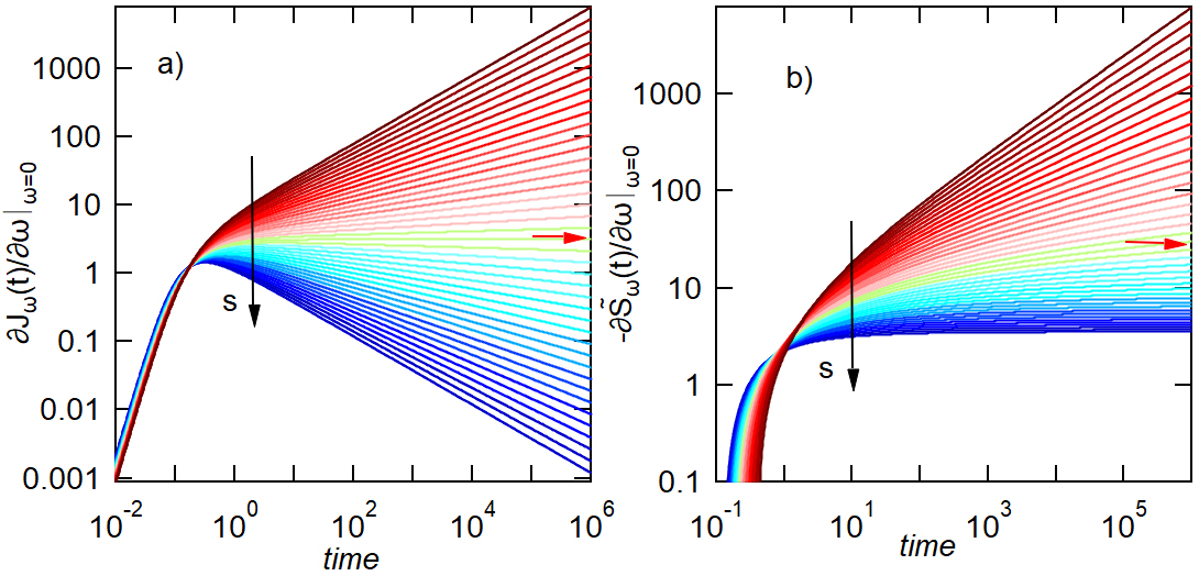
Figure 1: The derivatives of the spectral and principal density divided by $\lambda^{2}$ versus time. The derivatives are interpreted as the number of soft bosons emitted into the bath in the asymptotic limit and the number in the ground state, respectively. $s$ varies the interval $0.5\leq s\leq 1.5$ in increments of $0.025$ from top to bottom. Red arrow points to the ohmic bath values.

Figs. 1 (a) and (b) display the zero frequency derivatives of the time-dependent spectral and principal densities versus time of the dynamics, as a function of $s$. At $t\to\infty$, $\partial{\mathcal{J}}/\partial\omega|_{\omega=0}$ approaches zero, a constant, and infinity, if $s>1$, $s=1$, and $s<1$, respectively. In contrast, $\partial\tilde{\mathcal{S}}/\partial\omega|_{\omega=0}$ approaches a constant dependent on $s$ when $s>1$, and infinity when $s\leq 1$.

Taking the limit $t\to\infty$ in Eq. 27, we obtain the explicit derivatives of the spectral and principal densities at $\omega=0$:

$$\frac{\partial\tilde{\mathcal{J}}_{\omega}^{\alpha}}{\partial\omega}\bigg{|}_{\omega=0} = \left\{\begin{array}[]{ll}0,&\hbox{$s>1$;}\\ \pi\lambda^{2},&\hbox{$s=1$;}\\ \infty,&\hbox{$s<1$.}\end{array}\right.$$ (32)

$$\frac{\partial\tilde{\mathcal{S}}_{\omega}^{\alpha}}{\partial\omega}\bigg{|}_{\omega=0} = \left\{\begin{array}[]{ll}-2\lambda^{2}\Gamma(s)/(s-1),&\hbox{$s>1$;}\\ \infty,&\hbox{$s\leq 1$.}\end{array}\right.$$ (35)

Recall from the discussion below Eq. 15, that the derivative in Eq. 32 is valid at arbitrary temperature, but Eq. 35 is not.

II.2 Number of Emitted Soft Bosons

Let us establish a connection between the number of emitted soft bosons in the bath at zero temperature and the spectral density. In quantum field theory, the number of emitted bosons is closely related to the problem of asymptotic completeness [64]. Essentially, in order to prove asymptotic completeness, it is important to show that the number of bosons released into the bath is limited, since otherwise, the asymptotic states would not be in the Fock space [64].

Consider the small system initially in an excited eigenstate with a Bohr frequency $\epsilon>0$. During the time interval $t$ that fulfills $1/\epsilon<t<1/(|A_{21}|^{2}\tilde{\mathcal{J}}_{\epsilon})$, the population of the excited state is decreased by $|A_{21}|^{2}\tilde{\mathcal{J}}_{\epsilon}t$ according to the Fermi golden rule. $\epsilon|A_{21}|^{2}\tilde{\mathcal{J}}_{\epsilon}t$ is the resulting energy emitted into the bath. The number of emitted bosons is determined by dividing by $\epsilon$ using $|A_{21}|\sim 1$ in our units, i.e., $\langle N_{sb}(t)\rangle\sim\tilde{\mathcal{J}}_{\epsilon}t\sim t\epsilon\tilde{\mathcal{J}}_{\epsilon}/\epsilon$. By taking the limits $\epsilon\to 0_{+}$, $t\to+\infty$, and $\epsilon t=\text{const}$, we find the soft-boson number $\langle N_{sb}(\infty)\rangle\approx\partial\tilde{\mathcal{J}}_{\omega}/\partial\omega|_{\omega=0}$. On the other hand, Eq. 35 gives the boson number in the bath in the combined system-bath ground state. See Appendix B for further details.

Roeck and Kupiainen computed rigorous boson number bounds in scattering systems relaxing to unique states at zero temperature using a polymer expansion in statistical physics [64]. At time $t>0$, they find

$$\langle e^{\kappa N(t)}\rangle\leq\left\{\begin{array}[]{ll}\breve{C}\exp(C),&\hbox{$s\geq 1$};\\ \breve{C}\exp[Ct^{(1-s)}],&\hbox{$s<1$},\end{array}\right.$$ (36)

where $N(t)$ is the number of emitted bosons. $\breve{C}$ and $C$ are independent of $\lambda$, $\kappa$ and $t$, if $0<\lambda\leq\lambda_{0}$ and $|\kappa|\leq\kappa_{0}$, for some $\lambda_{0}>0$ and $\kappa_{0}>0$.

On the other hand, we have the asymptotic behavior from Eq. 27 at time $t\gg 1/\omega_{c}$,

$$\frac{\partial\tilde{\mathcal{J}}_{\omega}^{\alpha}(t)}{\partial\omega}\bigg{|}_{\omega=0} \mapsto \left\{\begin{array}[]{ll}\frac{2\lambda^{2}\Gamma(s+1)\sin\frac{(1-s)\pi}{2}}{1-s}\frac{1}{(\omega_{c}t)^{s-1}},&\hbox{$s>1$;}\\ \pi\lambda^{2}(1-\frac{2}{\pi\omega_{c}t}),&\hbox{$s=1$;}\\ \frac{2\lambda^{2}\Gamma(s+1)\sin\frac{(1-s)\pi}{2}}{1-s}(\omega_{c}t)^{1-s},&\hbox{$s<1$.}\end{array}.\right.$$ (40)

Comparing this with Eq. 36, along with the previous paragraph showing that $\partial\tilde{\mathcal{J}}_{\omega}^{\alpha}/\partial\omega|_{\omega=0}$ is the soft boson number at $t\to+\infty$, suggests that $\partial\tilde{\mathcal{J}}_{\omega}^{\alpha}(t)/\partial\omega|_{\omega=0}$ is the number of soft bosons that have been emitted up to time $t$. We shall see that the TCL4 master equation’s generator is linear with $\partial\tilde{\mathcal{J}}_{\omega}^{\alpha}(t)/\partial\omega|_{\omega=0}$. Consequently, the boson number determines both the asymptotic completeness and the existence of the generator of the TCL master equation.

The primary outcome of the work is the following theorem. If we assume that the open quantum system is generic, the states are computed up to the fourth order of the perturbation theory, the interaction $\lambda$ is arbitrarily small but not zero, and the thermodynamic limit is conventional, then, as a function of the dispersion $s$, we have

Theorem 1: The asymptotic states undergo a discontinuous phase transition, whereas the ground states undergo a continuous phase transition at $s=1$.

Outline of the proof: We will demonstrate in Sec. IV.1 that the reduced asymptotic states at $T=0$K are linear with $\partial\tilde{\mathcal{J}}/\partial\omega$ and independent of $\partial\tilde{\mathcal{S}}/\partial\omega$. Consequently, Eq. 32 represents a discontinuous transition from a bounded to an unbounded reduced asymptotic state, which takes place when $s$ changes from $1$ to $1_{-}$. The transition is consistent with the discontinuous transition in the boson number bound 36. The norm of the asymptotic state is the order parameter representing the discontinuous transition of the asymptotic state out of the Fock space.

In Sec. IV.2 we will show that the reduced ground states are linear with $\partial\tilde{\mathcal{S}}/\partial\omega$. Consequently, Eq. 35 represents a continuous transition from a bounded to an unbounded reduced ground state, which takes place when $s$ approaches $1_{+}$.

III TCL4 Generator

The system and the bath are initialized into a factorized state at time $t=0$. If the resulting quantum-dynamical map is invertible, it may be represented by the exact time-convolutionless master equation as follows [70]:

$$\frac{d\rho}{dt}=\mathcal{R}^{(0)}\rho+\mathcal{R}^{(2)}(t)\rho+\mathcal{R}^{(4)}(t)\rho+...$$ (41)

The generator of the dynamics is thus expressed in terms of tensors $\mathcal{R}^{(2n)}(t)$, each proportional to $\lambda^{2n}$. This will be the TCL2n master equation when it is truncated to the first $2n$ terms. Due to the hermiticity preservation of the master equation, the generator’s contributions can be written as

$$\mathcal{R}_{nm,ij}^{(2k)}(t)=\delta\mathcal{R}_{nm,ij}^{(2k)}(t)+\delta\mathcal{R}_{mn,ji}^{(2k)\star}(t),k=0,1,2,...$$ (42)

The matrix elements of the generator components are:

$$\delta\mathcal{R}_{nm,ij}^{(0)} = -iE_{n}\delta_{ni}\delta_{mj}$$ (43)

$$\delta\mathcal{R}_{nm,ij}^{(2)}(t) = \sum_{\alpha=1}^{N_{b}}\big{[}A_{ni}^{\alpha}A_{jm}^{\alpha}\Gamma_{in}^{\alpha}(t)$$ (44)

$$- \delta_{jm}\sum_{k=1}^{N}A_{nk}^{\alpha}A_{ki}^{\alpha}\Gamma_{ik}^{\alpha}(t)\big{]}.$$

$$\delta\mathcal{R}_{nm,ij}^{(4)}(t) = \sum_{a,b,c=1}^{N}\sum_{\alpha,\beta=1}^{N_{b}}\Big{\{}A_{na}^{\alpha}A_{ab}^{\beta}A_{bc}^{\alpha}A_{ci}^{\beta}\delta_{jm}[\mathsf{F}_{cb,ci,ac}^{\alpha\beta}(t)-\mathsf{R}_{cb,ab,bi}^{\alpha\beta}(t)]+A_{na}^{\alpha}A_{ab}^{\beta}A_{bc}^{\beta}A_{ci}^{\alpha}\delta_{jm}\mathsf{R}_{ic,ab,bi}^{\alpha\beta}(t)$$ (45)

$$- A_{na}^{\alpha}A_{ab}^{\alpha}A_{bc}^{\beta}A_{ci}^{\beta}\delta_{jm}\mathsf{F}_{ba,ci,ac}^{\alpha\beta}(t)-A_{na}^{\beta}A_{ab}^{\alpha}A_{bi}^{\beta}A_{jm}^{\alpha}[\mathsf{F}_{ba,bi,nb}^{\alpha\beta}(t)-\mathsf{R}_{ba,na,ai}^{\alpha\beta}(t)]$$ (46)

$$+ A_{na}^{\alpha}A_{ab}^{\beta}A_{bi}^{\beta}A_{jm}^{\alpha}\mathsf{F}_{an,bi,nb}^{\alpha\beta}(t)-A_{na}^{\beta}A_{ab}^{\beta}A_{bi}^{\alpha}A_{jm}^{\alpha}\mathsf{R}_{ib,na,ai}^{\alpha\beta}(t)$$ (47)

$$+ A_{na}^{\alpha}A_{ab}^{\alpha}A_{bi}^{\beta}A_{jm}^{\beta}[\mathsf{C}_{ba,jm,ai}^{\alpha\beta}(t)+\mathsf{R}_{ba,jm,ai}^{\alpha\beta}(t)]-A_{na}^{\alpha}A_{ab}^{\beta}A_{bi}^{\alpha}A_{jm}^{\beta}[\mathsf{C}_{ib,jm,ai}^{\alpha\beta}(t)+\mathsf{R}_{ib,jm,ai}^{\alpha\beta}(t)]$$ (48)

$$- A_{na}^{\alpha}A_{ai}^{\beta}A_{jb}^{\beta}A_{bm}^{\alpha}[\mathsf{C}_{an,jb,ni}^{\alpha\beta}(t)+\mathsf{R}_{an,jb,ni}^{\alpha\beta}(t)]+A_{na}^{\beta}A_{ai}^{\alpha}A_{jb}^{\beta}A_{bm}^{\alpha}[\mathsf{C}_{ia,jb,ni}^{\alpha\beta}(t)+\mathsf{R}_{ia,jb,ni}^{\alpha\beta}(t)]\Big{\}},$$ (49)

$$\mathsf{F}_{\omega_{1}\omega_{2}\omega_{3}}^{\alpha\beta}(t) = -\int_{0}^{t}d\tau\Delta\Gamma_{\omega_{1}}^{\alpha}(t,\tau)\Delta\Gamma_{\omega_{2}}^{\beta T}(t,t-\tau)e^{-i(\omega_{1}+\omega_{2}+\omega_{3})\tau}+i\Gamma_{\omega_{2}}^{\beta T}(t)\frac{\Gamma_{-\omega_{2}-\omega_{3}}^{\alpha}(t)-\Gamma_{\omega_{1}}^{\alpha}(t)}{\omega_{1}+\omega_{2}+\omega_{3}}$$ (50)

$$\mathsf{C}_{\omega_{1}\omega_{2}\omega_{3}}^{\alpha\beta}(t) = -\int_{0}^{t}d\tau\Delta\Gamma_{\omega_{1}}^{\alpha}(t,\tau)\Delta\Gamma_{\omega_{2}}^{\beta\star}(t,t-\tau)e^{-i(\omega_{1}+\omega_{2}+\omega_{3})\tau}+i\Gamma_{\omega_{2}}^{\beta\star}(t)\frac{\Gamma_{-\omega_{2}-\omega_{3}}^{\alpha}(t)-\Gamma_{\omega_{1}}^{\alpha}(t)}{\omega_{1}+\omega_{2}+\omega_{3}}$$ (51)

$$\mathsf{R}_{\omega_{1}\omega_{2}\omega_{3}}^{\alpha\beta}(t) = -\int_{0}^{t}d\tau\Delta\Gamma_{\omega_{1}}^{\alpha}(t,\tau)\Delta\Gamma_{\omega_{2}}^{\beta}(t,\tau)e^{-i(\omega_{1}+\omega_{2}+\omega_{3})\tau}+i\Gamma_{\omega_{2}}^{\beta}(t)\frac{\Gamma_{-\omega_{2}-\omega_{3}}^{\alpha}(t)-\Gamma_{\omega_{1}}^{\alpha}(t)}{\omega_{1}+\omega_{2}+\omega_{3}}.$$ (52)

Here

$$\Delta\Gamma_{\omega}^{\alpha}(t,\tau)=\Gamma_{\omega}^{\alpha}(t)-\Gamma_{\omega}^{\alpha}(\tau).$$ (53)

Eqs. 50-52 define the system’s 3D-spectral densities. On lines 45-49, $\mathsf{F}_{(ab)(cd)(ef)}^{\alpha\beta}(t)=\mathsf{F}_{\omega_{1}\omega_{2}\omega_{3}}^{\alpha\beta}(t)$, where $\omega_{1}=\omega_{ab}$, $\omega_{2}=\omega_{cd}$, and $\omega_{3}=\omega_{ef}$; mutadis mutandis $\mathsf{C}$ and $\mathsf{R}$. The superscript $T$ in Eq. 50 represents transposition in the energy basis, e.g., $\Delta\Gamma_{\omega_{2}}^{\beta T}=\Delta\Gamma_{-\omega_{2}}^{\beta}$. The star in the superscript in Eq. 51 indicates complex conjugation.

Once we have the time-dependent spectral density, we can express both the second and fourth-order contributions in terms of that spectral density. Therefore, the TCL4 master equations, in this particular form, has the same level of universality as the TCL2 master equation. The TCL4 master equation is trickier to use because we have to integrate over the products of the time-dependent spectral densities in equations Eqs. 50-52. Nevertheless, this may be simply managed through numerical computations. The integrals may be computed with a moderate amount of diligence, approaching double-precision accuracy, as we shall elaborate on in Section IV.3 After calculating the integrals, we may modify the system operators without the need to recalculate the 3D-spectral densities, resulting in faster computing.

The right-hand side (RHS) of Eqs. 50-52 should be interpreted as a limit in the case of $\omega_{1}+\omega_{2}+\omega_{3}=0$, i.e.,

$$\lim_{\Sigma_{i}\omega_{i}\to 0}\frac{\Gamma_{-\omega_{2}-\omega_{3}}^{\alpha}(t)-\Gamma_{\omega_{1}}^{\alpha}(t)}{\omega_{1}+\omega_{2}+\omega_{3}}=-\frac{\partial\Gamma_{\omega_{1}}^{\alpha}(t)}{\partial\omega_{1}}.$$ (54)

III.1 Asymptotic TCL4 Generator

In the thermodynamic limit, we substitute the smooth function from Eq. 27 for the spectral density. Then, the analytical characteristics of the TCL4 generator can be different from those of the TCL2 generator, because they depend on the derivative of the SD. In particular, Eqs. 32-35 are infrared divergent in a sub-ohmic bath leading to a diverging generator and diverging asymptotic state.

Let us consider the baths in the thermodynamic limit. According to the definition in Eq. 53, $\Delta\Gamma_{\omega}^{\alpha}(t,\tau)$ and $\Delta\Gamma_{\omega}^{\beta T}(t,t-\tau)$ vary from $\Gamma_{\omega}^{\alpha}(t)$ to $0$ and from $0$ to $\Gamma_{\omega}^{\beta T}(t)$, respectively, when $\tau$ changes from $0$ to $t$. If now we take the asymptotic limit, e.g., $t\to\infty$, then $\Delta\Gamma_{\omega}^{\alpha}(t,\tau)\to\Delta\Gamma_{\omega}^{\alpha}(\tau)=\Gamma_{\omega}^{\alpha}-\Gamma_{\omega}^{\alpha}(\tau)$, which approaches zero when $\tau$ is larger than the characteristic time scale of the bath. Vice versa, $\Delta\Gamma_{\omega}^{\beta T}(t,t-\tau)$ approaches zero when $\tau$ is smaller than $t$ minus the characteristic time scale of the bath, when $t$ is very large. As a result, we have

$$\lim_{t\to\infty}\Delta\Gamma_{\omega_{1}}^{\alpha}(t,\tau)\Delta\Gamma_{\omega_{2}}^{\beta T}(t,t-\tau)=0,\forall\tau\in[0,t].$$ (55)

The same applies after replacing $\Delta\Gamma_{\omega_{2}}^{\beta T}$ with $\Delta\Gamma_{\omega_{2}}^{\beta\star}$ in the above. Furthermore, we propose

$$\lim_{t\to\infty}\int_{0}^{t}d\tau\,\Delta\Gamma_{\omega_{1}}^{\alpha}(t,\tau)\Delta\Gamma_{\omega_{2}}^{\beta T}(t,t-\tau)e^{-i(\omega_{1}+\omega_{2}+\omega_{3})\tau}=0,$$ (56)

for $s>1/2$, and the same for $\Delta\Gamma_{\omega_{2}}^{\beta\star}$. See Appendix D for the proof of Eqs. 55 and 56 and $s>1/2$ as their region of validity.

In the asymptotic limit of Eqs. 50-52, we have the asymptotic 3D spectral densities,

$$\mathsf{F}_{\omega_{1}\omega_{2}\omega_{3}}^{\alpha\beta} = i\Gamma_{\omega_{2}}^{\beta T}\frac{\Gamma_{-\omega_{2}-\omega_{3}}^{\alpha}-\Gamma_{\omega_{1}}^{\alpha}}{\omega_{1}+\omega_{2}+\omega_{3}}$$ (57)

$$\mathsf{C}_{\omega_{1}\omega_{2}\omega_{3}}^{\alpha\beta} = i\Gamma_{\omega_{2}}^{\beta\star}\frac{\Gamma_{-\omega_{2}-\omega_{3}}^{\alpha}-\Gamma_{\omega_{1}}^{\alpha}}{\omega_{1}+\omega_{2}+\omega_{3}}$$ (58)

$$\mathsf{R}_{\omega_{1}\omega_{2}\omega_{3}}^{\alpha\beta} = i\Gamma_{\omega_{2}}^{\beta}\frac{\Gamma_{-\omega_{2}-\omega_{3}}^{\alpha}-\Gamma_{\omega_{1}}^{\alpha}}{\omega_{1}+\omega_{2}+\omega_{3}}-$$ (59)

$$\int_{0}^{\infty} d\tau \Delta\Gamma_{\omega_{1}}^{\alpha}(\tau)\Delta\Gamma_{\omega_{2}}^{\beta}(\tau)e^{-i(\omega_{1}+\omega_{2}+\omega_{3})\tau}.$$ (60)

The asymptotic generator is made by replacing the time-dependent 3D spectral densities in equations 45 through 49 with their corresponding asymptotic limits.

We take note of the claim made by Karasev and Teretenkov that the TCL expansion was expressed without the use of any quadratures in time [60]. This suggests that the remaining integral in 60 can be further simplified. Future research will be conducted on this topic.

III.2 TCL4 Generator’s Convergence at T=0K.

At zero temperature, according to Eqs. 19 and 28, $\tilde{\Gamma}_{\omega}^{\alpha}=\tilde{\mathcal{J}}_{\omega}^{\alpha}+i\tilde{\mathcal{S}}_{\omega}^{\alpha}$ is continuous when $s>0$. However, at a positive temperature, the spectral density diverges at zero frequency if $s<1$ [68], as $1/\omega^{1-s}$. To keep the paper simple, we will narrow the scope of the convergence analysis to $T=0$ K only, and defer the analysis of the convergence at a positive temperature to a future publication.

We first determine the 3D spectral density existence condition. At $T=0$ K, we only need to find the convergence condition for the three ratios in Eqs. 57-59. That is, we can ignore the integral in 60 for the time being because it will converge more quickly than the ratios. See appendix D for the justification of this claim.

As a result, the three ratios diverge if and only if $\omega_{1}+\omega_{2}+\omega_{3}=0$. After taking the limit $t\to\infty$ in Eq. 54,

$$\frac{\tilde{\Gamma}_{-\omega_{2}-\omega_{3}}^{\alpha}-\tilde{\Gamma}_{\omega_{1}}^{\alpha}}{\omega_{1}+\omega_{2}+\omega_{3}}=-\frac{\partial\tilde{\Gamma}_{\omega_{1}}^{\alpha}}{\partial\omega_{1}}=-i\int_{0}^{\infty}dt\,t\tilde{C}_{\alpha}(t)e^{i\omega_{1}t}.$$ (61)

For the BCF that decays as $t^{-s-1}$, the integrand alternates in sign versus time at $\omega_{1}\neq 0$. In this case the integral exists under the original premise that $s>0$. However, if $\omega_{1}=0$, in addition to $\omega_{1}+\omega_{2}+\omega_{3}=0$, the integral will diverge if $s\leq 1$. This is the origin of the infrared divergence at $T=0$ K.

To assess the impact of the infrared divergence on the generator, we will isolate the contributions from the $\omega_{1}+\omega_{2}+\omega_{3}=0$ and $\omega_{1}=0$ terms in 45-49. In such terms, $\omega_{2}+\omega_{3}=0$ as well. After adding those terms up, we determined that the equation-lines 45-47 result in zero. In the remaining equation lines 48-49, the requirement $\omega_{2}+\omega_{3}=0$, for $\omega_{2}=\omega_{ab}$ and $\omega_{3}=\omega_{cd}$ splits into two possibilities: $(a=b\wedge c=d)\vee(a=d\wedge b=c)$. The diverging terms sum up to zero in the scenario where $a=b\wedge c=d$. However, the divergences corresponding to $a=d\wedge b=c$ do not cancel.

After adding the hermitian conjugate to Eq. 45 and some algebra, the sum of all the terms that can diverge for $s\leq 1$ is

$$\mathcal{R}_{nm,ij}^{(4,d)}(t)=2\delta_{ij}\sum_{\alpha\beta=1}^{N_{b}}\big{\{}i(A_{mm}^{\alpha}-A_{jj}^{\alpha})A_{nm}^{\alpha}|A_{mj}^{\beta}|^{2}\text{Im}[\mathsf{C}(t)+\mathsf{R}(t)]_{0,jm,mj}^{\alpha\beta}-i(A_{nn}^{\alpha}-A_{ii}^{\alpha})A_{nm}^{\alpha}|A_{ni}^{\beta}|^{2}\text{Im}[\mathsf{C}(t)+\mathsf{R}(t)]_{0,in,ni}^{\alpha\beta}\big{\}}.$$ (62)

The second term on the RHS of Eq. 62 is obtained from the first term through complex conjugation and realignment $n\leftrightarrows m$ and $i\leftrightarrows j$, ensuring the preservation of hermiticity defined in Eq. 42.

Due to the $\delta_{ij}$ on the RHS of Eq. 62, only the population-to-coherence transfer matrix elements $\mathcal{R}_{nm,ii}^{(4,d)}$ can diverge. It is easy to show that $\mathcal{R}_{nn,ii}^{(4,d)}(t)=0$, and thus $\mathcal{R}_{nn,ii}^{(4)}$ is bounded. Similarly, $\mathcal{R}_{ni,ni}^{(4,d)}(t)=0$ and thus $\mathcal{R}_{ni,ni}^{(4)}$ is bounded. Since the secular transfer rates $\mathcal{R}_{nn,ii}^{(4)}$ and $\mathcal{R}_{ni,ni}^{(4)}$ are all bounded, the fourth-order Davies master equation, as a result, does not have infrared divergence under the same conditions as the second-order Davies master equation. The expansion in higher-order Davies generators was discussed in [80, Sec. IV.C.1], which is consistent with this result.

When the ratios in Eqs. 51 and 52 are inserted into the equation for $\mathsf{C}+\mathsf{R}$, the real part in $\Gamma_{\omega}^{\beta}$ is isolated. In more precise terms, $\Gamma_{\omega}^{\beta}+\Gamma_{\omega}^{\beta\star}=2Re(\Gamma_{\omega}^{\beta})$. The result is

$$\text{Im}[\mathsf{C}(t)+\mathsf{R}(t)]_{0,in,ni}^{\alpha\beta} = \text{Im}\left\{-2i\text{Re}[\Gamma^{\beta}_{in}(t)]\frac{\partial\Gamma_{\omega}^{\alpha}(t)}{\partial\omega}\bigg{|}_{\omega=0}\right\}$$ (63)

$$= -2\mathcal{J}_{in}^{\beta}(t)\frac{\partial\mathcal{J}_{\omega}^{\alpha}(t)}{\partial\omega}\bigg{|}_{\omega=0}$$

Substituting into Eq. 62 for $i=j$, we obtain

$$\mathcal{R}_{nm,ii}^{(4,d)}(t) = -4i\sum_{\alpha\beta=1}^{N_{b}}\frac{\partial\mathcal{J}_{\omega}^{\alpha}(t)}{\partial\omega}\bigg{|}_{\omega=0}\bigg{[}$$ (65)

$$(A_{mm}^{\alpha}-A_{ii}^{\alpha})A_{nm}^{\alpha}\mathcal{J}_{im}^{\beta}(t)|A_{im}^{\beta}|^{2}$$

$$- (A_{nn}^{\alpha}-A_{ii}^{\alpha})A_{nm}^{\alpha}\mathcal{J}_{in}^{\beta}(t)|A_{in}^{\beta}|^{2}\bigg{]}.$$ (66)

The terms on lines 65 and 66 converge as $t\to\infty$ for any $s>0$. It follows that $\mathcal{R}_{nm,ii}^{(4,d)}(t)$ diverges if and only if the derivative of the real part of the spectral density diverges at $\omega=0$ (see line 65). Thus, the sufficient and necessary condition for the existence of the fourth-order asymptotic generator is

$$\frac{\partial\mathcal{J}_{\omega}^{\alpha}}{\partial\omega}\bigg{|}_{\omega=0}=-\int_{0}^{\infty}t\text{Im}[C(t)]dt<\infty.$$ (67)

Figure 2 illustrates the Fermi golden rule and the relaxation-dephasing hybrid processes (Eqs. 65-66) in a two-level system, which is initially in the excited state. The system relaxes into a quasistatic equilibrium state because the Fermi golden rule rate, sketched in Fig. 2(a), is initially much higher than the rate of the fourth-order hybrid process. But, the latter grows in time as soft bosons are emitted into the bath, and may out-compete the Fermi golden rule over a long time.

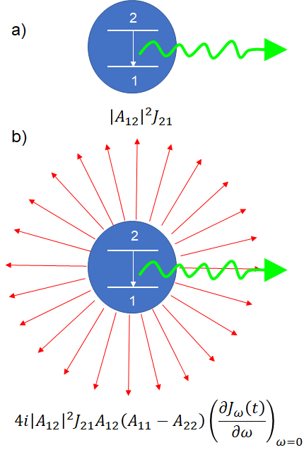
Figure 2: Soft boson emission in a two-level system. Picture (a) represents the Fermi golden rule for the relaxing system. The fourth-order relaxation-dephasing hybrid process is depicted in picture (b).

The dephasing sub-process of the hybrid process has probability proportional to the derivative of the spectral density at zero frequency at time $t$ and to $A_{12}(A_{11}-A_{22})$, from Eqs. 65-66. We mentioned before that the derivative is similar to the number of soft bosons emitted at time $t$. Overall, the system dynamics first reaches a quasistatic steady state at the Fermi-golden rule rate; however, when the soft boson number increases too fast, the global quantum state may exit the Fock space. Then, the density matrix computed in the Fock space diverges. We stress that the infrared divergence is from a mathematical problem: the Fock space incompleteness. It is an issue that may be resolved by mathematical techniques [65]. We do, however, welcome the generator’s irregularity.

The TCL4 generator is uniformly bounded in the interval $s\geq 1$, since the LHS of Eq. 67 is bounded according to Eq. 32. The condition 67 is temperature-independent (recall Eq. 11). The condition 67 is less stringent than the existence of Eq. 61, where the derivatives of the real and imaginary parts must both be bounded to guarantee that the 3D spectral functions are bounded.

IV Approach to a ground state 

As an application, we examine if and how the open quantum system dynamics approaches the combined system and bath ground state. Our method for calculating the asymptotic and ground states will be detailed in the next two parts.

IV.1 Asymptotic States

Here, we use the perturbation theory of the asymptotic TCL4 generator to compute the corrections to the system’s asymptotic dynamics. The working hypothesis will be that the asymptotic limit exists for $s\geq 1$.

Let us begin with the master Eq. 41, which can be rewritten in the asymptotic limit as

$$\frac{d\rho(t)}{dt}=\mathcal{R}^{(0)}\rho(t)+\lambda^{2}\mathcal{R}^{(2)}\rho(t)+\lambda^{4}\mathcal{R}^{(4)}\rho(t)+...$$ (68)

For clarity, the generator’s explicit dependency on $\lambda$ has been excised as a prefactor in each term of the expansion. Since the coefficients of this equation are time-independent, we seek the solution $\rho(t)=e^{\nu t}\rho$, which leads to the linear system

$$(\mathcal{R}^{(0)}+\lambda^{2}\mathcal{R}^{(2)}+\lambda^{4}\mathcal{R}^{(4)}+...)\rho=\nu\rho,$$ (69)

with the unknowns $\nu$ and $\rho$. We will solve this eigenvalue equation using the perturbation theory, which is sometimes referred to as the canonical perturbation theory (CPT). This method has been applied to explore the asymptotic states in Refs. [15, 16].

$\nu$ and $\rho$ are expanded in the Taylor series as $\nu=\nu^{(0)}+\lambda^{2}\nu^{(2)}+\lambda^{4}\nu^{(4)}+...$ and $\rho=\rho^{(0)}+\lambda^{2}\rho^{(2)}+\lambda^{4}\rho^{(4)}+...$. Inserting in the eigenvalue equation 69, we find

$$(\mathcal{R}^{(0)}+\lambda^{2}\mathcal{R}^{(2)}+\lambda^{4}\mathcal{R}^{(4)}+...)(\rho^{(0)}+\lambda^{2}\rho^{(2)}+\lambda^{4}\rho^{(4)}+...)\\ =(\nu^{(0)}+\lambda^{2}\nu^{(2)}+\lambda^{4}\nu^{(4)}+...)(\rho^{(0)}+\lambda^{2}\rho^{(2)}+\lambda^{4}\rho^{(4)}+...).$$ (70)

Expanding the requirement $\text{tr}\rho=1$ in Taylor series in $\lambda$, we find

$$\text{tr}\rho^{(2k)}=\delta_{k0}.$$ (71)

Next, we equalize the coefficients of the expansion on the LHS and the RHS of Eq. 70. In the zeroth order and using Eq. 43, we find

$$-i\omega_{nm}\rho_{nm}^{(0)}=\nu^{(0)}\rho_{nm}^{(0)},$$ (72)

where $\omega_{nm}=E_{n}-E_{m}$. Since we assume that the eigenenergies of the isolated system are nondegenerate, it follows that there are $N^{2}-N$ nondegenerate eigenvalues $-i\omega_{nm},n\neq m$, with the eigenvectors equal to the coherences $\rho=|n\rangle\langle m|$. In addition, there is a zero eigenvalue with a degenerate manifold of populations $\rho=|n\rangle\langle n|,n=1,2,...,N$.

The application of the Fermi golden rule on the Liouvillian operating in the representation of the algebra of local operators shows that $N^{2}-1$ of these $N^{2}$ eigenvalues disintegrate in the continuous spectrum when the interaction is turned on [67], which leads to return to equilibrium. In our case, the reduced system’s Liouvillian retains a fully discrete spectrum. Proceeding with the perturbation theory, in the second order, we find

$$\mathcal{R}^{(2)}\rho^{(0)}+\mathcal{R}^{(0)}\rho^{(2)}=\nu^{(2)}\rho^{(0)}+\nu^{(0)}\rho^{(2)}.$$ (73)

The examination of the coherences, while intriguing on its own, does not offer any data directly pertinent to the results of this work and will be skipped.

The population corrections are computed using degenerate perturbation theory. We have $\nu^{(0)}=0$ and consider the superpositions $\rho^{(0)}=\sum_{k=1}^{N}\rho_{kk}^{(0)}|k\rangle\langle k|$. Then let us take the matrix element $\langle n|...|m\rangle$ of Eq. 73. The result is

$$\sum_{k=1}^{N}\mathcal{R}^{(2)}_{nm,kk}\rho_{kk}^{(0)}-i\omega_{nm}\rho_{nm}^{(2)}=\nu^{(2)}\rho_{nn}^{(0)}\delta_{nm}.$$ (74)

For $n=m$, we find

$$\sum_{k=1}^{N}\mathcal{R}^{(2)}_{nn,kk}\rho_{kk}^{(0)}=\nu^{(2)}\rho_{nn}^{(0)},$$ (75)

which is the usual eigenvalue problem in degenerate perturbation theory.

Let us make a few remarks. First, it should be noted that 75 determines both the eigenvalues $\nu^{(2)}$ and the populations $\rho_{nn}^{(0)}$ to precision $O(\lambda^{0})$. However, after multiplying $\nu^{(2)}$ with $\lambda^{2}$, the eigenvalues of the generator will be known to precision $O(\lambda^{2})$. Second, trace preservation of the master equation requires that $\sum_{k}\mathcal{R}_{kk,ij}^{(2q)}=0$. When we take the sum over $n$ in Eq. 75 we see that $\nu^{(2)}\sum_{k}\rho_{kk}^{(0)}=0$. If $\nu^{(2)}=0$, then $\sum_{k}\rho_{kk}^{(0)}$ can be nonzero. This eigenvector represents the reduced system’s asymptotic state in the zeroth order, which is unique by the condition 20. If $\nu^{(2)}\neq 0$, then $\sum_{k}\rho_{kk}^{(0)}=0$. These eigenvectors turn out to be the same as the decaying population modes in the Davies master equation [17]. There are $N-1$ such modes.

The nonsecular matrix elements of the generator will generate coherences in these modes. Let $n\neq m$ in Eq. 74. Then

$$\rho_{nm}^{(2)}=-\frac{i}{\omega_{nm}}\sum_{k=1}^{N}\mathcal{R}_{nm,kk}^{(2)}\rho_{kk}^{(0)}.$$ (76)

Thus from the $O(\lambda^{2})$ generator, the coherences are known to precision $O(\lambda^{2})$.

At this time, the coherences are more precise than the populations, which is one of the flaws of the Redfield equation. To make the precision of the populations consistent with the coherences, we must look at the populations’ fourth-order corrections, where we have

$$\mathcal{R}^{(0)}\rho^{(4)}+\mathcal{R}^{(2)}\rho^{(2)}+\mathcal{R}^{(4)}\rho^{(0)}=\nu^{(4)}\rho^{(0)}+\nu^{(2)}\rho^{(2)}.$$ (77)

Taking the matrix element $\langle n|...|m\rangle$, this equation transforms into

$$-i\omega_{nm}\rho_{nm}^{(4)} + \sum_{i,j=1}^{N}\mathcal{R}^{(2)}_{nm,ij}\rho_{ij}^{(2)}+\sum_{k=1}^{N}\mathcal{R}^{(4)}_{nm,kk}\rho_{kk}^{(0)}$$ (78)

$$= \nu^{(4)}\delta_{nm}\rho_{nn}^{(0)}+\nu^{(2)}\rho_{nm}^{(2)}.$$

Take $n=m$ to obtain the next in-order population correction. We have the following linear system

$$\sum_{k=1}^{N}\left[\mathcal{R}^{(2)}_{nn,kk}-\nu^{(2)}\delta_{nk}\right]\rho_{kk}^{(2)}=\nu^{(4)}\rho_{nn}^{(0)}$$ (79)

$$- \sum_{i,j=1}^{N}{}^{{}^{\prime}}\mathcal{R}^{(2)}_{nn,ij}\rho_{ij}^{(2)}-\sum_{k=1}^{N}\mathcal{R}^{(4)}_{nn,kk}\rho_{kk}^{(0)}.$$

The primed sum indicates summations over unequal indices $i$ and $j$. Both the fourth-order corrections of the relaxation rates and the second-order corrections of the populations are generated by this equation.

The key finding is that the second-order populations depend on $\mathcal{R}^{(4)}_{nn,kk}$. So, in order to compute the population dynamics to precision $O(\lambda^{2})$ of the TCL2-generator, we must compute the population-to-population matrix elements of the TCL4 generator. This discovery extends the findings of [15, 16] from asymptotic states to asymptotic dynamics. See Appendix E for the Redfield equation’s dynamics inaccuracy at times longer than the relaxation time.

Let us summarize the corrections for the asymptotic state, which can be obtained by substitution $\nu^{(0)}=\nu^{(2)}=...=0$ in all of the above equations. For the coherences, $i\neq j$, we find

$$\rho^{(0)}_{ij} = 0,$$ (80)

$$\rho^{(2)}_{ij} = \frac{-i}{\omega_{ij}}\sum_{k=1}^{N}\mathcal{R}^{(2)}_{ij,kk}\rho^{(0)}_{kk},$$ (81)

$$\rho^{(4)}_{ij} = \frac{-i}{\omega_{ij}}\Big{[}\sum_{k=1}^{N}(\mathcal{R}^{(2)}_{ij,kk}\rho^{(2)}_{kk}+\mathcal{R}^{(4)}_{ij,kk}\rho^{(0)}_{kk})$$ (82)

$$+ \sum_{l,m=1}^{N}{}^{{}^{\prime}}\mathcal{R}^{(2)}_{ij,lm}\rho^{(2)}_{lm}\Big{]},$$

while for the populations, we have

$$\sum_{k=1}^{N}\mathcal{R}^{(2)}_{nn,kk}\rho^{(0)}_{kk} = 0$$ (83)

$$\sum_{k=1}^{N}\mathcal{R}^{(2)}_{nn,kk}\rho^{(2)}_{kk} = -\sum_{k=1}^{N}\mathcal{R}^{(4)}_{nn,kk}\rho^{(0)}_{kk}$$ (84)

$$- \sum_{l,m=1}^{N}{}^{{}^{\prime}}\mathcal{R}^{(2)}_{nn,lm}\rho^{(2)}_{lm}$$

$$\sum_{k=1}^{N}\mathcal{R}^{(2)}_{nn,kk}\rho^{(4)}_{kk} = -\sum_{k=1}^{N}(\mathcal{R}^{(6)}_{nn,kk}\rho^{(0)}_{kk}+\mathcal{R}^{(4)}_{nn,kk}\rho^{(2)}_{kk})$$ (85)

$$- \sum_{k,l=1}^{N}{}^{{}^{\prime}}(\mathcal{R}^{(4)}_{nn,kl}\rho^{(2)}_{kl}+\mathcal{R}^{(2)}_{nn,kl}\rho^{(4)}_{kl}).$$

At zero temperature, inserting Eq. 44 into Eq. 83 and applying Eq. 71, we find the solution $\rho_{kk}^{(0)}=\delta_{k1}$, which is simply the statement that the zeroth-order asymptotic reduced state is the ground state of the isolated system.

Now it is clear that the infrared divergence of the TCL4 generator directly leads to the asymptotic state divergence when $s$ is less than $1$. We have not computed the matrix elements $\mathcal{R}^{(6)}_{nn,kk}$. However, these may be found in the limited asymptotic states [80, Sec.IV.C.1] of the 6th order Davies master equation. Therefore, the relaxation-dephasing hybrids within $\mathcal{R}^{(4)}_{nm,ii}$ can be the only source of divergence in Eqs. 80-85. For example, the term $\rho_{ij}^{(4)}$ will diverge at zero temperature if and only if $\mathcal{R}^{(4)}_{ij,11}$ diverges; which is the case if and only if, in the limit $t\to\infty$, $\partial\mathcal{J}/\partial\omega|_{\omega=0}$ diverges. Further, line  85 demonstrates that $\rho_{kk}^{(4)}$ diverges if $\rho_{kl}^{(4)}$ diverges and $\mathcal{R}^{(2)}_{nn,kl}$ is nonzero. Thus we have shown the first part of Theorem 1, that the divergence in the asymptotic states depends linearly on $\partial\mathcal{J}/\partial\omega|_{\omega=0}$.

IV.2 Ground States

To make the discussion easier, let us proceed with the assumption that there is only one bath. Nondegenerate Rayleigh-Schrödinger perturbation theory will be used to determine the ground state of the whole Hamiltonian, which is nondegenerate for the free Hamiltonian. After that, we will take the thermodynamic limit, to be consistent with how we determine the genrators. Recently, Cresser and Andrés adapted this method to the second-order Rayleigh-Schrd̈inger perturbation theory [81], which we now extend to the fourth-order.

We are attempting to calculate the ground state’s reduced density matrix. That is, we are assuming that the perturbed (coupled) Hamiltonian $\tilde{H}=H_{0}+\lambda V$ has a ground state $|\tilde{0}\rangle$ that can be expanded in powers of $\lambda$, and $|\tilde{0}\rangle=|0\rangle+O(\lambda^{1})$. From this total ground state approximation, we will then calculate the reduced density matrix for just the system part, that is,

$$\tilde{\varrho}_{S}=\text{Tr}_{B}|\tilde{0}\rangle\langle\tilde{0}|.$$

In the zeroth order, the ground state of the free Hamiltonian is the tensor product of the ground states of the system and the bath. See Appendix F for the derivation of the second- and fourth-order corrections of the ground state. Reducing the ground state of the total system to the density matrix of the system, we find the second-order corrections

$$\rho_{\text{mfgs},nn}^{(2)} = -|A_{nn}|^{2}\partial\tilde{\mathcal{S}}_{1n},\hbox{$n=2,3,..,N$;}$$ (86)

$$\rho_{\text{mfgs},ij}^{(2)} = \frac{A_{i1}A_{1j}(\tilde{\mathcal{S}}_{1i}-\tilde{\mathcal{S}}_{1j})}{E_{i}-E_{j}}$$ (87)

$$+ \sum_{k}\frac{(\delta_{1i}A_{1k}A_{kj}-\delta_{1j}A_{ik}A_{k1})\tilde{\mathcal{S}}_{1k}}{E_{i}-E_{j}},$$

where $\tilde{\mathcal{S}}_{1k}=\tilde{\mathcal{S}}_{\omega_{1k}}$ and $\partial\tilde{\mathcal{S}}_{ab}=\partial\tilde{\mathcal{S}}(\omega)/\partial\omega$ at $\omega=\omega_{ab}$. Here mfgs refers to the mean-force ground state, which is equivalent to the mean-force Gibbs state at zero temperature. Alternatively, the mean-force ground state is the reduced ground state of the combined system and bath.

These findings are identical to [81] after applying the Kramers-Kronig transform $\tilde{\mathcal{S}}\mapsto\tilde{\mathcal{J}}$. There is a bounded perturbative ground state in the second order of the coupling at any $s>0$.

The perturbative corrections of the reduced ground state coherences in the fourth order of coupling are

$$\rho_{\text{mfgs},ij}^{(4)}=\sum_{a,b=1}^{N}\frac{A_{ib}A_{b1}A_{1a}A_{aj}}{\omega_{1i}\omega_{1j}}\tilde{\mathcal{S}}_{1a}\tilde{\mathcal{S}}_{1b}-\sum_{a=1}^{N}\Big{[}A_{1a}A_{a1}A_{i1}A_{1j}\frac{\tilde{\mathcal{S}}_{1a}(\partial\tilde{\mathcal{S}}_{1i}-\partial\tilde{\mathcal{S}}_{1j})+\partial\tilde{\mathcal{S}}_{1a}(\tilde{\mathcal{S}}_{1i}-\tilde{\mathcal{S}}_{1j})}{\omega_{ij}}\Big{]}$$ (88)

$$+ \sum_{a=1}^{N}\sum_{b=2}^{N}(A_{i1}A_{1a}A_{ab}A_{bj}+A_{ib}A_{ba}A_{a1}A_{1j})\frac{\tilde{\mathcal{S}}_{1a}(\tilde{\mathcal{S}}_{1j}-\tilde{\mathcal{S}}_{1i})}{\omega_{b1}\omega_{ij}}$$

$$+ \sum_{a=1}^{N}\sum_{b=2}^{N}(A_{i1}A_{1a}A_{ab}A_{bj}+A_{ib}A_{ba}A_{a1}A_{1j})\frac{\tilde{\mathcal{S}}_{{1a}}}{\omega_{ij}}\int_{-\infty}^{\infty}\frac{d\omega^{\prime}}{\pi}\frac{\tilde{\mathcal{J}}_{\omega^{\prime}}}{(\omega_{ab}-\omega^{\prime})}\left[\frac{1}{(\omega_{1j}-\omega^{\prime})}-\frac{1}{(\omega_{1i}-\omega^{\prime})}\right]$$

$$+ \sum_{a=1}^{N}\sum_{b=1}^{N}A_{ib}A_{b1}A_{aj}A_{1a}\frac{\tilde{\mathcal{S}}_{{1a}}}{\omega_{ij}}\int_{-\infty}^{\infty}\frac{d\omega^{\prime}}{\pi}\frac{\tilde{\mathcal{J}}_{\omega^{\prime}}}{(\omega_{1b}-\omega^{\prime})}\left[\frac{1}{(\omega_{aj}-\omega^{\prime})}-\frac{1}{(\omega_{ai}-\omega^{\prime})}\right]$$

$$- \sum_{a=1}^{N}\sum_{b=1}^{N}A_{ib}A_{b1}A_{aj}A_{1a}\frac{1}{\omega_{ij}}\int_{-\infty}^{\infty}\frac{d\omega^{\prime}}{\pi}\left[\frac{\tilde{\mathcal{J}}_{\omega^{\prime}}\tilde{\mathcal{S}}_{{1j}-\omega^{\prime}}}{(\omega_{1b}-\omega^{\prime})(\omega_{1a}-\omega^{\prime})}-\frac{\tilde{\mathcal{J}}_{\omega^{\prime}}\tilde{\mathcal{S}}_{{1j}-\omega^{\prime}}}{(\omega_{1b}-\omega^{\prime})(\omega_{aj}-\omega^{\prime})}\right]+h.c.$$

$$- \sum_{a=1}^{N}\sum_{b=1}^{N}(A_{i1}A_{1a}A_{ab}A_{bj}+A_{ib}A_{ba}A_{a1}A_{1j})\frac{1}{\omega_{ij}}\int_{-\infty}^{\infty}\frac{d\omega^{\prime}}{\pi}\left[\frac{\tilde{\mathcal{J}}_{\omega^{\prime}}\tilde{\mathcal{S}}_{\omega_{1b}-\omega^{\prime}}}{(\omega_{1j}-\omega^{\prime})(\omega_{ab}-\omega^{\prime})}-\frac{\tilde{\mathcal{J}}_{\omega^{\prime}}\tilde{\mathcal{S}}_{\omega_{1b}-\omega^{\prime}}}{(\omega_{1j}+\omega^{\prime})(\omega_{1a}+\omega^{\prime})}\right]+h.c.$$

$$\hbox{$i,j=2,3,...,N$;$i\neq j$}.$$

The derivative $\partial\tilde{\mathcal{S}}$ is present on the first line, as well as certain cases of both the third and fourth lines, demonstrating that both $\partial\tilde{\mathcal{S}}$ as well as $\tilde{\mathcal{S}}$ govern the ground states. According to Eq. 35, $\partial\tilde{\mathcal{S}}$ at zero frequency diverges in the limit $s\to 1_{+}$. Isolating the terms in the summations in  88 that contain this derivative, we find

$$\rho_{\text{mfgs},ij}^{(4)} = \ldots+A_{11}\left(A_{i1}A_{1j}A_{11}-|A_{i1}|^{2}A_{ij}\right)$$ (89)

$$\times \left(\frac{\tilde{\mathcal{S}}_{\omega_{1i}}\partial\tilde{\mathcal{S}}_{0}}{\omega_{ij}}+\int_{-\infty}^{\infty}\frac{d\omega^{\prime}}{\pi}\frac{\tilde{\mathcal{J}}_{\omega^{\prime}}\tilde{\mathcal{S}}_{\omega_{1i}-\omega^{\prime}}}{\omega_{ij}(\omega^{\prime})^{2}}\right)$$

$$- A_{i1}A_{1j}A_{11}\left(A_{11}-A_{jj}\right)$$

$$\times \left(\frac{\tilde{\mathcal{S}}_{\omega_{1j}}\partial\tilde{\mathcal{S}}_{0}}{\omega_{ij}}+\int_{-\infty}^{\infty}\frac{d\omega^{\prime}}{\pi}\frac{\tilde{\mathcal{J}}_{\omega^{\prime}}\tilde{\mathcal{S}}_{\omega_{1j}-\omega^{\prime}}}{\omega_{ij}(\omega^{\prime})^{2}}\right)$$

As a result, the fourth-order correction to the coherence $\rho_{\text{mfgs},ij}^{(4)}$ diverges continuously in the limit $s\to 1_{+}$ due to the term $\partial\tilde{\mathcal{S}}_{0}$ given by Eq. 35. See Appendix F for the terms $\rho_{\text{mfgs},1j}^{(4)}$, which also diverge due to the term $\partial\tilde{\mathcal{S}}_{0}$. This completes the proof of the second claim stated in Theorem 1 that the function $\partial\tilde{\mathcal{S}}/\partial\omega|_{\omega=0}$ controls the divergence of the reduced ground state.

IV.3 Approach to precision $O(\lambda^{2})$

In the traditional thermodynamic limit method, it is relatively easy to show and widely known that the ground state coherences provided by Eq. 87 and the coherences of the asymptotic solutions of the TCL2 master equation are identical [15, 82, 16, 83, 84]. However, establishing the identity of the second-order populations is substantially more challenging. Recently, there has been some progress in finding a solution to this problem [84]. According to Eqs. 86 and 87, the ground state in the second order in $\lambda$ is bounded at any $s>0$. Since it solely depends on the secular matrix elements of the TCL4 generator, which are infrared regular, the asymptotic state populations determined using Eq. 85 are bounded too. Still, it is not evident how the asymptotic and ground-state populations are related.

Hänggi and coworkers hypothesized that the asymptotic coherences can be analytically continued into the asymptotic populations [82]. In that situation, they discovered agreement between the asymptotic and equilibrium states to precision $O(\lambda^{2})$. This is due to the fact that such analytical continuation holds true for the equilibrium states. In our case, when $i$ and $j$ are equal to $n$, it may be said that Eq. 86 is the limit of Eq. 87. Given that the asymptotic and the ground state coherences are identical, the analytical continuations of their coherences are clearly also identical. Therefore, the analytic continuation cannot provide new information until it can be demonstrated that it is applicable to asymptotic states. Here we numerically computed the second-order population corrections from the TCL4 generator, and compared them to the second-order corrections in the ground states using the following example.

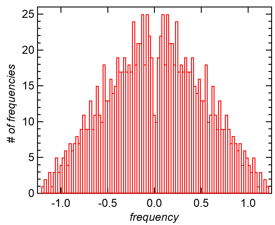
Figure 3: Histogram of Bohr frequency of the random-matrix example. $N=35$ In these units, the bath cut-off frequency is $\omega_{c}=10$

The system Hamiltonian has $N=35$ eigenenergies taken from the eigenvalue distribution of a Gaussian unitary ensemble of big matrices at the spectrum’s center (GUE). The histogram in Fig. 3 displays the Bohr frequency distribution. There are 1191 distinct Bohr frequencies, with 0.0114, 0.4194, and 1.2108 being the lowest, average, and greatest absolute oscillation frequency, respectively. The energy level repulsion, which prevents energy levels from being too close to one another, is what causes the minimum around 0 frequency. The bath cutoff frequency is $\omega_{C}=10$ the BCF-decay is ohmic ($s=1$), which gurantees the existance of the TCL4 generator. The vast number of frequencies is significant since it indicates our TCL4 generator’s capacity to account for a large plethora of frequencies. This will be useful when extending the generator to time-dependent system Hamiltonians.

For the system coupling operator, we randomly select an $N\times N$ hermitian matrix from the GUE. All levels of the system are connected by this matrix in a way that allows for direct relaxation between them. It also exhibits significant diagonal element fluctuations, indicating the existence of dephasing. We separated the integration region into sections before computing the integral in 60. Smaller time steps are employed when the integrand is big. We may accept larger time steps without compromising accuracy if the integrand is small.

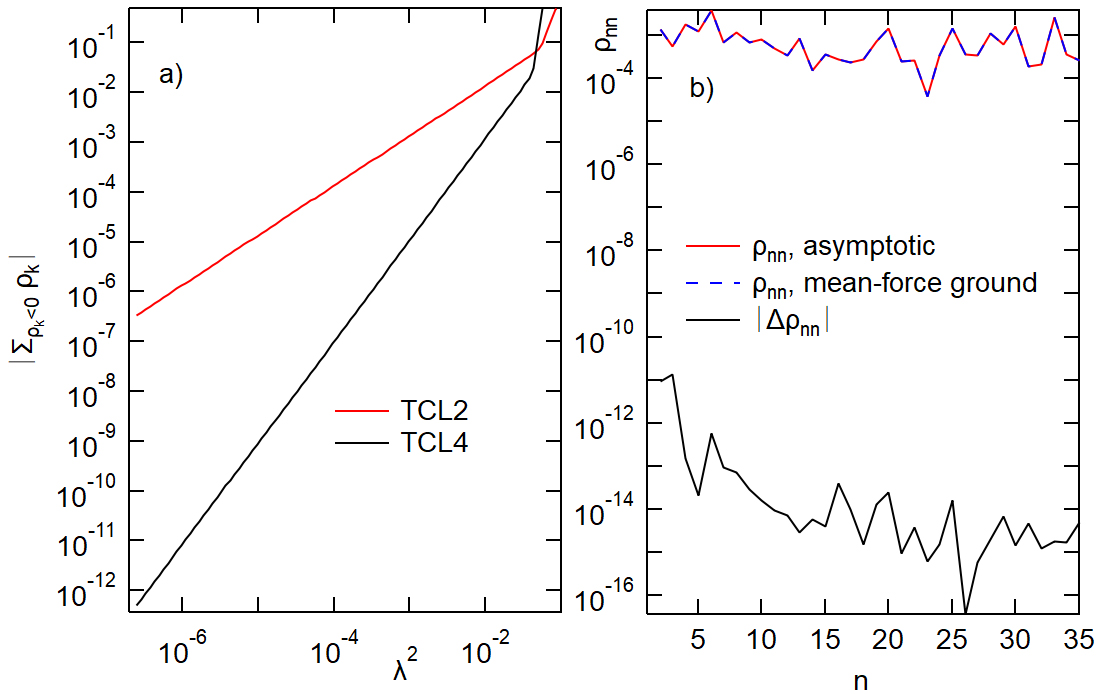
Figure 4: Asymptotic state properties in a 35-level system. a) Absolute negativity of the asymptotic density matrix versus coupling constant. b) Populations of the excited states $\rho_{nn}^{(2)}$ and the absolute value of the difference between the populations of the asymptotic and the reduced ground state versus $n$. $\omega_{c}=10$, $s=1$, $T=0$K.

The results for the asymptotic states in the ohmic bath at $T=0$K are shown in Fig. 4. In (a), we compute the absolute negativity, or the absolute sum of the negative eigenvalues of the asymptotic states of the TCL2 and TCL4 generators. The figure shows that the negativity scales as $\lambda^{2}$ and $\lambda^{4}$ in the TCL2 and TCL4 asymptotic states, respectively. The negativity also measures the state inaccuracy because the precise quantum state’s negativity must be zero. Therefore, the inaccuracy of the asymptotic states scales as $\lambda^{2}$ and $\lambda^{4}$, which is in agreement with the downgrade in accuracy of quantum master equations discussed by Fleming and Cummings [15]. The decrease in the negativity of the TCL4 asymptotic states relative to those of the TCL2 shows that all inaccuracies owing to the second order have been properly canceled out by the fourth order terms. So, the negativity may be used as a test to confirm that there are no algebraic errors in the TCL2n generators’ computation. The asymptotic states turn positive in the limit $n\to\infty$ since the time-convolutionless master equation is exact. This is implied here by the observation that the asymptotic state negativity seems to scale with $\lambda^{n}$, based on $n=1$ and $2$.

The second-order corrections of the asymptotic and ground state populations computed using Eqs. 84 and 86 are shown in Fig. 4(b). The difference between the corrections is approximately ten orders of magnitude smaller than the corrections. The similarity is unlikely to be coincidental and provides an additional proof that our calculation of the TCL4 generator is error-free. As a function of $N$, we have reached the limit of computing precision at $N=4$, where we discovered that the asymptotic and ground state populations agree in 13 significant digits (not shown).

Within the second-order perturbation theory, we can relax the working hypothesis $s\geq 1$, since the asymptotic states converge at any $s>0$. For $s=0.9,1.1$, and $1.2$, the 13-digit agreement was valid. In the open range $0<s<5$, we have likewise discovered numerical agreement; however, assuming the same computational bandwidth, the number of significant digits decreases dramatically when $s$ is much lower than one. This is due to the longer integration time required to achieve the necessary accuracy at lower $s$.

In summary, the reduced asymptotic state of a small open quantum is almost certainly identical to the reduced ground state computed in order of $O(\lambda^{2})$, in the entire physical range of baths ($s>0$). We believe that algebraic proof of this statement is within reach.

IV.4 Approach to a ground state to precision $O(\lambda^{4})$

Because the CPT requires the TCL6 generator to generate the asymptotic populations in the fourth order [15], we can only directly compare the coherences between the asymptotic and ground states in the fourth order, based on the work done so far. According to theorem 1, the asymptotic states of the TCL4 master equation have a first-order phase transition at $s=1$, represented by Eq. 32. On the other hand, the ground state coherences diverge continuously in the limit $s\to 1_{+}$ as $1/(s-1)$ according to Eqs. 35. Therefore, the asymptotic and ground states cannot be the same. Their distance is larger the closer $s$ approaches $1$ and diverges in the limit $s\to 1_{+}$.

The following asymptotic limits capture the approach to ground state in the zeroth and second order in $\lambda$ and its breakdown in the fourth order:

$$\lim_{t\to\infty}\|\rho_{\text{TCL4}}(t)-\rho_{\text{mfgs,0}}\| = O(\lambda^{2});s\geq 1,$$ (90)

$$\lim_{t\to\infty}\|\rho_{\text{TCL4}}(t)-\rho_{\text{mfgs,2}}\| = O(\lambda^{4});s\geq 1,$$ (91)

$$\lim_{t\to\infty}\|\rho_{\text{TCL4}c}(t)-\rho_{\text{mfgs,4c}}\| = O\left(\frac{\lambda^{4}}{s-1}\right);s>1,$$ (92)

where $\rho_{\text{mfgs,2k}}=\rho_{\text{mfgs}}^{(0)}+\lambda^{2}\rho_{\text{mfgs}}^{(2)}+...\lambda^{2k}\rho_{\text{mfgs}}^{(2k)}$, for $k=0,1$ and $2$. The inequality 92 is for the coherences of the ground and asymptotic states only, which are both computed with errors of order $O(\lambda^{6})$. Since their distance is of order $O(\lambda^{4})$ while the error of this distance is of order $O(\lambda^{6})$, the dynamics does not approach the ground state to precision $O(\lambda^{4})$.

Proof of Eqs. 90-92: Applying the perturbation theory, we have $\lim_{t\to\infty}\rho_{\text{TCL4}}(t)\equiv\tilde{\rho}=\tilde{\rho}^{(0)}+\lambda^{2}\tilde{\rho}^{(2)}+\lambda^{4}\tilde{\rho}^{(4)}+...$, which we substitute in the steady state equation for the TCL4 generator. Eqs. 80–85 result from this, however they lack the sixth and higher order terms. Since the sixth-order terms are absent from Eqs. 80-81 and 83-84, the solutions for $\tilde{\rho}^{(0)}$ and $\tilde{\rho}^{(2)}$ will match those found with the CPT, which also match the mean-force ground states based on the previous section. It follows that $\tilde{\rho}=\rho_{\text{mfgs,0}}+\lambda^{2}\rho_{\text{mfgs,2}}+\lambda^{4}\tilde{\rho}^{(4)}+...$

Moreover, since the TCL4 generator is bounded uniformly in $s$ when $s\geq 1$, $\tilde{\rho}^{(4)}$, as determined by Eqs. 82 and 85 (without the sixth and higher order terms), is bounded uniformly in $s$. Inserting $\tilde{\rho}$ in the LHSs of Eqs. 90 and 91, these equations are proven. The LHS of Eq. 92 yields $\lambda^{4}\|\tilde{\rho}^{(4)}_{c}-\rho_{\text{mfgs,c}}^{(4)}\|$ when $\tilde{\rho}$ is substituted, where subscript c indicates the coherence part of the density matrix. For $s\geq 1$, $\rho_{\text{mfgs,c}}^{(4)}$ is linear with $1/(s-1)$, as shown in Sec: IV.2, while $\tilde{\rho}^{(4)}_{c}$ is bounded uniformly in $s$. As a result, the bound 92 is proportional to $O(\lambda^{4})$ and is not uniform in $s$. QED.

  Counterexamples

We briefly discuss two nongeneric open quantum systems. If $(A^{\alpha}_{ii}-A^{\alpha}_{nn})A^{\alpha}_{nm}\mathcal{J}_{in}^{\beta}|A_{in}^{\beta}|^{2}=0$, $\forall i,n,\alpha,\beta$, equation lines 65 and 66 demonstrate that the TCL4 generator’s divergence at $s<1$ is suppressed. Consider for example the unbiased spin boson model , where $A=\sigma_{z}/2$ and $H_{S}=\sigma_{x}/2$, with $\sigma_{x}$ and $\sigma_{z}$, the Pauli sigma matrices. $A$ has no diagonal matrix elements in the energy eigenbasis, hence the TCL4 generator exhibits no infrared divergence for any $s>0$. In ohmic and sub-ohmic baths, ground states are known to exist for the unbiased spin boson model Hamiltonian [63, 77, 85, 86]. Theorem 1 does not apply.

Another example is the exactly solvable reduced dynamics of pure dephasing Hamiltonians where $[A,H_{S}]=0$. This dynamics converges at any $s>0$. There are no off-diagonal matrix elements in the energy eigenbasis of $A$. As a consequence, the TCL4 generator converges for any $s>0$. Again, theorem 1 does not apply. It is reassuring to know that in these two examples of infrared regular dynamics, the TCL4 generator is also infrared regular at zero temperature.

V Conclusion

In conclusion, for the fourth-order perturbative time-convolutionless quantum master equation, we provided a concise yet exact generator. The time-dependent spectral density of the bath and one integral over time must be determined before setting up the generator. As a result, this equation can now be used to study a variety of complex dynamical systems, without worrying about the inaccuracies that build up over the time scale comparable to the relaxation time. These systems may include glasses, conjugated polymers, light-harvesting biomolecular complexes, black holes, as well as quantum state preparation and gate fidelity.

As an application, we investigated the approach to ground state characteristics in rather large open quantum systems. The approach is numerically exact only in the second-order perturbation theory. The situation is considerably more complex in the fourth order, though. The system asymptotic and ground states are both present in super-ohmic baths, but they can differ significantly. The system’s asymptotic state is still present in ohmic bath, but the ground state is not perturbatively present. In contrast, the system initially stabilizes near a Fock space ground state in sub-ohmic bath, which is still present in the order of $O(\lambda^{2})$, but after an escape time, the generator approaches divergence and the the reduced state starts to diverge.

We expect the reformulated fourth-order time convolutionless master equation to pave the way for new approaches to solid-state quantum computing noise reduction at low frequencies [87, 88, 89, 90]. The ubiquitous $1/f$ noise and dephasing in these systems at very low temperatures clearly point to the necessity of an approach for open quantum systems at $T=0$K that takes soft bosons into account. Since it results from entanglement with soft bosons, which have unlimited wavelengths, the loss of phase coherence between qubits at finite distance may be correlated, which is beyond the control of quantum error correction. The TCL4 master equation could be an appropriate equation to explain correlated quantum noise.

In biomolecular light-harvesting complexes, low-frequency noise and structured spectral noise are also prevalent. The absence of diverging density matrices in the experiments on these systems does not necessarily mean that the infrared problem is not relevant. Long-lasting coherences in exciton-energy transfer in photosynthetic light harvesting are inexplicable [2]. The coherences have been attributed to the alignment between the structured spectral densities in the protein environment and the Bohr frequencies of the small excitonic system [91]. However, the question of if and how Darwinian evolution results in spectral synchronization remains unanswered.

We greatly appreciate the insightful comments that Anton Trushechkin, Marco Merkli, Michael Loss, Brian Kennedy, Itamar Kimchi, Sami Hakani and Oliver Dial provided. We acknowledge support from the School of Physics at the Georgia Institute of Technology.

Appendix A KMS and the Kramers-Kronig relations.

In this section we rewrite the spectral functions of the finite sized system-bath in terms of the sums over discrete bath modes, as opposed to the integrals over frequency. In the main text, we introduced a highly irregular spectral density function Eq. 10 and expressed the generators in terms of that function, so that the thermodynamic limit can be performed simply by replacing the irregular spectral density with the smooth function 19. Here we convert the integrals back to the sums over discrete bath modes and demonstrate that the key relationships in Sec. II hold without the assumption 19.

The BCF of the finite sized combined system, corresponding to Eq. 11 translates to

$$C_{\alpha}(t)=\sum_{k}(g_{k}^{\alpha})^{2}[\cos(\omega_{k}^{\alpha}t)\coth(\beta_{\alpha}\omega_{k}^{\alpha}/2)-i\sin(\omega_{k}^{\alpha}t)].$$ (93)

The time-dependent spectral density given by Eq. 12 recasts as

$$\Gamma_{\omega}^{\alpha}(t) = \int_{0}^{t}d\tau C_{\alpha}(\tau)e^{i\omega\tau}$$

$$= \sum_{k}(g_{k}^{\alpha})^{2}\int_{0}^{t}d\tau e^{i\omega\tau}[e^{i\omega_{k}^{\alpha}\tau}f_{k}^{\alpha}+e^{-i\omega_{k}^{\alpha}\tau}(1+f_{k}^{\alpha})].$$

where $f_{k}^{\alpha}=1/(e^{\beta_{\alpha}\omega_{k}^{\alpha}}-1)$. Performing the integral over time, and taking the real and imaginary parts, we obtain

$$\mathcal{J}_{\omega}^{\alpha}(t)=\sum_{k}(g_{k}^{\alpha})^{2}\Big{[}\frac{\sin(\omega+\omega_{k}^{\alpha})t}{\omega+\omega_{k}^{\alpha}}f_{k}^{\alpha}\\ +\frac{\sin(\omega-\omega_{k}^{\alpha})t}{\omega-\omega_{k}^{\alpha}}(1+f_{k}^{\alpha})\Big{]}\\ \mathcal{S}_{\omega}^{\alpha}(t)=\sum_{k}(g_{k}^{\alpha})^{2}\big{[}\frac{1-\cos(\omega+\omega_{k}^{\alpha})t}{\omega+\omega_{k}^{\alpha}}f_{k}^{\alpha}\\ +\frac{1-\cos(\omega-\omega_{k}^{\alpha})t}{\omega-\omega_{k}^{\alpha}}(1+f_{k}^{\alpha})\big{]}.$$ (95)

These are the spectral functions that the TCL2n generators depend on. Neither the asymptotic ($t\to\infty$) nor the thermodynamic ($L\to\infty$) limits have been applied.

Let us now take the limit $t\to\infty$ in Eq. 95 before the thermodynamic limit. Using the representation of the delta function, e.g., $\delta(y)=\lim_{x\to\infty}\sin(xy)/(\pi y)$, we get the asymptotic spectral density

$$\mathcal{J}_{\omega}^{\alpha}=\pi\sum_{k}(g_{k}^{\alpha})^{2}\Big{[}\delta(\omega+\omega_{k}^{\alpha})f_{k}^{\alpha}+\delta(\omega-\omega_{k}^{\alpha})(1+f_{k}^{\alpha})\Big{]}$$ (96)

At $\omega>0$, we can drop the left delta-function since $\omega_{k}^{\alpha}\geq 0$. Using the general property $\delta(x-y)h(x)=\delta(x-y)h(y)$, we can pull $(1+f_{k}^{\alpha})$ as $1+f(\omega)$ in front of the sum, where $f(\omega)=1/[\exp(\beta_{\alpha}\omega)-1]$. This results in the relation 16. Using similar manipulations, at $\omega<0$, this equation reproduces the KMS condition 17.

We can rewrite the principal density at time $t$ in Eq. 95 as

$$\mathcal{S}_{\omega}^{\alpha}(t)=\frac{1}{\pi}\int_{0}^{\infty}d\omega^{\prime}\leavevmode\nobreak\ \tilde{\mathcal{J}}_{\omega^{\prime}}^{\alpha}\big{[}\frac{1-\cos(\omega+\omega^{\prime})t}{\omega+\omega^{\prime}}f(\omega^{\prime})\\ +\frac{1-\cos(\omega-\omega^{\prime})t}{\omega-\omega^{\prime}}(1+f(\omega^{\prime})\big{]}.$$ (97)

Changing the variable on the first line $\omega^{\prime}\to-\omega^{\prime}$, and utilizing the relations 16 and 17, we find

$$\mathcal{S}_{\omega}^{\alpha}(t)=\frac{1}{\pi}\int_{-\infty}^{\infty}d\omega^{\prime}\mathcal{J}_{\omega^{\prime}}^{\alpha}\frac{1-\cos(\omega-\omega^{\prime})t}{\omega-\omega^{\prime}}.$$ (98)

This equation is an extension of the Kramers-Kronig relation to the time dependent spectral density. The ratio in the integrand is regular at $\omega=\omega^{\prime}$. We can thus pull a principal value in front of the integral, with the understanding that the integration region excludes an infinitesimal interval $[\omega-\epsilon,\omega+\epsilon]$ only, e.g., the singularities of the delta functions within $\mathcal{J}_{\omega}^{\alpha}$ do not count under the principal value. Then, we take the limit $t\to\infty$ and apply the Rieman-Lebesgue lemma. This results in the Kramers-Kronig relation 18.

Appendix B Boson Numbers in the van Hove and pure dephasing hamiltonians.

Let us take a look at the boson numbers in the ground and asymptotic states of the van Hove [92] and pure dephasing hamiltonians [70], where these can be calculated exactly.

For the van Hove hamiltonian, we take $H_{S}=0$, $N_{b}=1$, and $A=1$. We rewrite the hamiltonian in Eq. 1 as

$$H_{T}=\sum_{k}\omega_{k}(b_{k}+\frac{g_{k}}{\omega_{k}})^{\dagger}(b_{k}+\frac{g_{k}}{\omega_{k}})-\sum_{k}\frac{g_{k}^{2}}{\omega_{k}},$$ (99)

by ‘completing the square’. The ground state is a displaced vacuum with the oscillator displacements $\alpha_{k}=-g_{k}/\omega_{k}$. The ground state energy is

$$E_{g}=\frac{1}{\pi}\int_{0}^{\infty}d\omega\frac{\tilde{\mathcal{J}}}{\omega}\mapsto 2\pi\lambda^{2}\Gamma(s)\omega_{c},$$ (100)

where, recall that $\mapsto$ means taking the thermodynamic limit. It is bounded if and only if $s>0$. The average boson number is

$$\langle N\rangle=\sum_{k}\frac{g_{k}^{2}}{\omega_{k}^{2}}=\frac{1}{\pi}\int_{0}^{\infty}d\omega\frac{\tilde{\mathcal{J}}(\omega)}{\omega^{2}}\mapsto-\frac{\partial\tilde{\mathcal{S}}}{\partial\omega}\bigg{|}_{\omega=0}.$$ (101)

The last equality can be shown by integrating by parts (e.g., $\int udv=uv-\int vdu$, where $u=\tilde{\mathcal{J}},dv=d\omega/\omega^{2}$), and replacing $\tilde{\mathcal{J}}$ and $\tilde{\mathcal{S}}$ with $\partial\tilde{\mathcal{J}}/\partial\omega$ and $\partial\tilde{\mathcal{S}}/\partial\omega$, respectively, in the Kramers-Kronig equation 18. This assumes that $\tilde{\mathcal{J}}(\omega)/\omega=0$ at $\omega=0$, $\partial\tilde{\mathcal{J}}/\partial\omega<\infty$, and $\partial\tilde{\mathcal{S}}/\partial\omega<\infty$, all of which holds true for the spectral density in Eq. 19 if $s>1$.

Next, we compute the dynamics at $T=0K$. The annihilation operators in the Heisenberg picture satisfy the equation of motion,

$$\frac{db_{k}}{dt}=i[H_{T},b_{k}]=-i\omega_{k}b_{k}-ig_{k},$$ (102)

which has the solution

$$b_{k}(t)=b_{k}(0)e^{-i\omega_{k}t}-\frac{g_{k}}{\omega_{k}}(1-e^{-i\omega_{k}t}).$$ (103)

In the Heisenberg picture the bath is in the vacuum state $|0\rangle$. Thus, $b_{k}(t)|0\rangle=\alpha_{k}(t)|0\rangle$, where $\alpha_{k}(t)=-(g_{k}/\omega_{k})(1-e^{-i\omega_{k}t})$. After rotating back to the Schrödinger picture, the bath state, $\exp(-iH_{T}t)|0\rangle$, is the displaced vacuum with the oscillator displacements $\alpha_{k}(t)$. The state of the small system does not change while the bath is being displaced because the Hilbert space of the system is one dimensional.

The average boson number is

$$\langle N(t)\rangle=\sum_{k}|\alpha_{k}(t)|^{2}=\frac{2}{\pi}\int_{0}^{\infty}d\omega\frac{\tilde{\mathcal{J}}(\omega)}{\omega^{2}}[1-\cos(\omega t)]$$ (104)

$$\mapsto 4\lambda^{2}\Gamma(s-1)\left\{1-\frac{\cos[(s-1)\arctan(\omega_{c}t)]}{(1+\omega_{c}^{2}t^{2})^{\frac{s-1}{2}}}\right\}.$$

The number of bosons grows as $|t|^{1-s}$ for $s<1$ and as $\log(t)$ at $s=1$. For $s>1$, the boson number is bounded uniformly in time.

Taking the limits $t\to\infty$ and $L\to\infty$ on the first line of Eq. 104, (in arbitrary order), applying the Riemann–Lebesgue lemma, and integrating by parts as described below Eq. 101, we find

$$\lim_{t\to\infty}\langle N(t)\rangle=-2\frac{\partial\tilde{\mathcal{S}}}{\partial\omega}\bigg{|}_{\omega=0};s>1.$$ (105)

By Eq. 35, the ground and asymptotic state boson numbers both diverge as $1/(s-1)$ in the limit $s\to 1_{+}$.

Eqs. 35, 101, and 105 show that the hamiltonian admits both asymptotic and ground states, if and only if $s>1$. No infrared divergence is present in the system’s reduced dynamics since there is no dynamics. Extension to pure dephasing hamiltonians yields similar boson numbers [70, Sec. 4.2]. In this case, we can take $H_{s}=0$ and $A=\sigma_{z}$ (Pauli $\sigma$-matrix). Once again, the diverging boson numbers at $s\leq 1$ have no impact on the dynamics. Pure dephasing hamiltonians do not satisfy the Fermi golden rule condition 2 in Sec. II.

Appendix C Derivation of the TCL4 generator

Let us begin with [55, Eq. (29)] as the expression of the TCL4 generator in the interaction picture,

$$\Big{(}\frac{\partial\varrho}{\partial t}\Big{)}_{4}=\sum_{\alpha,\beta=1}^{N_{b}}\int_{0}^{t}dt_{1}\int_{0}^{t_{1}}dt_{2}\int_{0}^{t_{2}}dt_{3}\big{\{}\langle 02\rangle_{\alpha}\langle 13\rangle_{\beta}[\hat{0}^{\alpha},[\hat{1}^{\beta},\hat{2}^{\alpha}]\hat{3}^{\beta}\varrho]\\ -\langle 02\rangle_{\alpha}\langle 31\rangle_{\beta}[\hat{0}^{\alpha},[\hat{1}^{\beta},\hat{2}^{\alpha}]\varrho\hat{3}^{\beta}]+\langle 03\rangle_{\alpha}\langle 12\rangle_{\beta}([\hat{0}^{\alpha},[\hat{3}^{\alpha},\hat{2}^{\beta}]\varrho\hat{1}^{\beta}]+[\hat{0}^{\alpha},[\hat{1}^{\beta}\hat{2}^{\beta},\hat{3}^{\alpha}]\varrho])\\ -\langle 03\rangle_{\alpha}\langle 21\rangle_{\beta}[\hat{0}^{\alpha},[\hat{1}^{\beta},\hat{3}^{\alpha}]\varrho\hat{2}^{\beta}]\big{\}}+h.c.$$ (106)

Where we have expanded the authors’ original short-hand notation to account for our to our multiple uncorrelated baths, defining $\hat{i}^{\alpha}=A^{\alpha}(t_{i})$ and $\langle ij\rangle_{\alpha}=C_{\alpha}(t_{i}-t_{j})$ with $i=0,\ldots,3$ where $t_{0}=t$. We have omitted the explicit time dependence of the reduced density matrix as well, defining $\varrho=\varrho(t)$, the interaction picture operator.

C.1 Integral Simplification

For finite $t$, the integration in Eq. (106) is over a bounded region in $D\subset\mathbb{R}^{3}$.

Let us consider three general operators,

$$K_{ijk}^{\alpha\beta} =\langle 0i\rangle_{\alpha}\langle jk\rangle_{\beta}[\hat{0}^{\alpha},[\hat{i}^{\alpha},\hat{k}^{\beta}]\varrho\hat{j}^{\beta}]$$ (107)

$$H_{ijk}^{\alpha\beta} =\langle 0i\rangle_{\alpha}\langle jk\rangle_{\beta}[\hat{0}^{\alpha},[\hat{j}^{\beta}\hat{k}^{\beta},\hat{i}^{\alpha}]\varrho]$$ (108)

$$M_{ijk}^{\alpha\beta} =\langle 0i\rangle_{\alpha}\langle jk\rangle_{\beta}[\hat{0}^{\alpha},\hat{j}^{\beta}[\hat{i}^{\alpha},\hat{k}^{\beta}]\varrho]$$ (109)

with which we can rewrite Eq. (106) as

$$\Big{(}\frac{\partial\varrho}{\partial t}\Big{)}_{4}=\sum_{\alpha,\beta=1}^{N_{b}}\int_{0}^{t}dt_{1}\int_{0}^{t_{1}}dt_{2}\int_{0}^{t_{2}}dt_{3}\big{(}K_{231}^{\alpha\beta}+H_{213}^{\alpha\beta}\\ +M_{213}^{\alpha\beta}+K_{321}^{\alpha\beta}+K_{312}^{\alpha\beta}+H_{312}^{\alpha\beta}\big{)}+h.c.$$ (110)

Note that the variables $t_{1},t_{2},t_{3}$ are independent, and that for any two successive integrals, we can visualize the region of integration as a triangle in $\mathbb{R}^{2}$. Assuming the integral is bounded, we can change the order of integration as

$$\int_{0}^{t_{n-1}}dt_{n}\int_{0}^{t_{n}}dt_{n+1}\mapsto\int_{0}^{t_{n-1}}dt_{n+1}\int_{t_{n+1}}^{t_{n-1}}dt_{n}$$ (111)

We will use this to transform the integral over $D$. Our choice of transformation will depend only on the order of the time arguments within the bath correlation functions, which we separate into two cases, $i=2$ and $i=3$. Let us also employ the short-hand notation

$$\int_{0}^{i}d_{j}=\int_{0}^{t_{i}}dt_{j}$$ (112)

Case 1 ($i=2$):

$$\iiint_{D}=\int_{0}^{t}d_{1}\int_{0}^{1}d_{2}\int_{0}^{1}d_{3}\\ +\int_{0}^{t}d_{3}\int_{0}^{3}d_{2}\int_{0}^{3}d_{1}-\int_{0}^{t}d_{3}\int_{0}^{3}d_{2}\int_{0}^{t}d_{1}$$ (113)

and we have

Case 2 ($i=3$):

$$\iiint_{D}=\int_{0}^{t}d_{2}\int_{0}^{t}d_{1}\int_{0}^{2}d_{3}-\int_{0}^{t}d_{2}\int_{0}^{2}d_{1}\int_{0}^{2}d_{3}$$ (114)

While the overall ordering of the time arguments is not arbitrary, as long as the relation between the scalar correlation functions and the and operator product ordering is preserved with the $\alpha,\beta$ bath index labels, we are free to swap the arbitrary $t_{1},t_{2},t_{3}$ labels. Thus, we will permute the labels such that the bounds only depend on time $t_{1}$ as the outermost integration variable. Applying, we arrive at a simplified form of Eq. (110),

$$\begin{split}\Big{(}\frac{\partial\varrho}{\partial t}\Big{)}_{4}=\sum_{\alpha,\beta=1}^{N_{b}}\Big{\{}\int_{0}^{t}dt_{1}\int_{0}^{t_{1}}dt_{3}\int_{0}^{t_{1}}dt_{2}\left(Q_{213}^{\alpha\beta}+M_{231}^{\alpha\beta}\right)\\ +\int_{0}^{t}dt_{1}\int_{0}^{t}dt_{3}\int_{0}^{t_{1}}dt_{2}P_{231}^{\alpha\beta}\Big{\}}+h.c.\end{split}$$ (115)

Where we have defined two new functions

$$Q_{ijk}^{\alpha,\beta} =H_{ijk}^{\alpha,\beta}+M_{ijk}^{\alpha,\beta}=\langle 0i\rangle_{\alpha}\langle jk\rangle_{\beta}[\hat{0}^{\alpha},[\hat{j}^{\beta},\hat{i}^{\alpha}]\hat{k}^{\beta}\varrho]$$ (116)

$$P_{ijk}^{\alpha,\beta} =K_{ijk}^{\alpha,\beta}-M_{ijk}^{\alpha,\beta}=\langle 0i\rangle_{\alpha}\langle jk\rangle_{\beta}[\hat{0}^{\alpha},[\hat{j}^{\beta},[\hat{k}^{\beta},\hat{i}^{\alpha}]\varrho]]$$ (117)

We will also define the double integrals of our remaining functions as,

$$\mathcal{Q}^{\alpha\beta}(t,t_{1}) =\int_{0}^{t_{1}}dt_{2}\int_{0}^{t_{1}}dt_{3}Q^{\alpha\beta}_{213}$$ (118a)

$$\mathcal{P}^{\alpha\beta}(t,t_{1}) =\int_{0}^{t_{1}}dt_{2}\int_{0}^{t}dt_{3}P^{\alpha\beta}_{231}$$ (118b)

$$\mathcal{M}^{\alpha\beta}(t,t_{1}) =\int_{0}^{t_{1}}dt_{2}\int_{0}^{t_{1}}dt_{3}M^{\alpha\beta}_{231}$$ (118c)

Our goal now is to write Eq. (115) as single quadrature,

$$\begin{split}\Big{(}\frac{\partial\varrho}{\partial t}\Big{)}_{4}=\sum_{\alpha,\beta=1}^{N_{b}}\int_{0}^{t}dt_{1}[\mathcal{Q}^{\alpha\beta}(t,t_{1})+\mathcal{P}^{\alpha\beta}(t,t_{1})\\ +\mathcal{M}^{\alpha\beta}(t,t_{1})]+h.c.\end{split}$$ (119)

by evaluating the integrals in Eq. (118), which can be expressed in terms of products of system operators and the time-dependent spectral density for each bath, $\Gamma^{\alpha}_{\omega}(t)$, defined in Eq. 12.

C.2 Time-Dependent Spectral Density

As mentioned in the main text, we assume that for each bath the BCF has the property $C_{\alpha}(-s)=C_{\alpha}^{*}(s)$, from which we can define the complex conjugate of $\Gamma^{\alpha}_{\omega}(t)$ as

$$\Gamma^{\alpha*}_{\omega}(t)=\int_{0}^{t}dsC_{\alpha}^{*}(s)e^{-i\omega s}=-\Gamma^{\alpha}_{\omega}(-t)$$ (120)

We define transposition as $\Gamma^{\alpha T}_{\omega}(t)=\Gamma^{\alpha}_{-\omega}(t)$, since we will be evaluating the function only for the Bohr frequencies, which can be expressed in terms of the system energies as $\omega_{nm}=E_{n}-E_{m}$, leading to an antisymmetric matrix representation in the $H_{S}$ eigenbasis, $\omega_{mn}^{T}=-\omega_{mn}$. With these two operations, we have a hermitian conjugate, $\Gamma^{\alpha\dagger}_{\omega}(t)=-\Gamma^{\alpha}_{-\omega}(-t)$.

We will define a Hadamard product in the system energy basis which is equivalent to a point wise product in the frequency domain,

$$f\circ g=f(\omega_{nm})g(\omega_{nm})=f_{\omega}g_{\omega}.$$ (121)

With this product we can express the interaction picture operators as

$$\hat{i}^{\alpha}=A^{\alpha}(t_{i})=U^{\dagger}(t_{i})A^{\alpha}U(t_{i})=A^{\alpha}\circ e^{i\omega t_{i}}.$$ (122)

Where $A^{\alpha}$ is a time-independent hermitian system coupling operator, and $U(t)$ is the unitary time evolution operator $U(t)=e^{-i\hat{H}_{S}t}$.

To evaluate (118), we could rotate each expression to the Schrödinger picture, expand each coefficient in the system energy basis, in which can we would find that each bath index contributes an integral of one of the following forms,

$$\int_{t_{a}}^{t_{b}}dsC(t-s)e^{i\omega s} =e^{i\omega t}\Delta\Gamma^{T}_{\omega}(t-t_{a},t-t_{b})$$ (123a)

$$\int_{t_{a}}^{t_{b}}dsC(s-t)e^{i\omega s} =e^{i\omega t}\Delta\Gamma_{\omega}^{*}(t-t_{a},t-t_{b}),$$ (123b)

where we have use the Eq. 44 definition of $\Delta\Gamma_{\omega}(t,\tau)$.

However, examining the operators $P^{\alpha\beta}_{213},Q^{\alpha\beta}_{213},M^{\alpha\beta}_{231}$, we note that since only a single system operator will depend on $t_{2}$ and $t_{3}$, we can use the linearity of integration and the linearity of operators themselves to see that the results of 123 can be accounted for while still in the interaction picture using

$$\int_{t_{a}}^{t_{b}}dt_{j}\langle ij\rangle_{\alpha}\hat{j}^{\alpha} =\hat{i}^{\alpha}\circ\Delta\Gamma^{\alpha T}(t_{i}-t_{a},t_{i}-t_{b})$$ (124a)

$$\int_{t_{a}}^{t_{b}}dt_{j}\langle ji\rangle_{\alpha}\hat{j}^{\alpha} =\hat{i}^{\alpha}\circ\Delta\Gamma^{\alpha*}(t_{i}-t_{a},t_{i}-t_{b}).$$ (124b)

Where we have removed frequency subscript, as it is determined by the product. Equations 124 define our “Hadamard trick", which enables fast evaluation of the TCL4 generator kernels over the different integration regions.

Explicitly evaluating 118, we find

$$\mathcal{Q}^{\alpha\beta}(t,t_{1}) =\int_{0}^{t_{1}}dt_{2}\int_{0}^{t_{1}}dt_{3}\langle 02\rangle_{\alpha}\langle 13\rangle_{\beta}[\hat{0}^{\alpha},[\hat{1}^{\beta},\hat{2}^{\alpha}]\hat{3}^{\beta}\varrho]=[\hat{0}^{\alpha},[\hat{1}^{\beta},\{\hat{0}^{\alpha}\circ\Delta\Gamma^{\alpha T}(t,t-t_{1})\}]\{\hat{1}^{\beta}\circ\Delta\Gamma^{\beta T}(t_{1},0)\}\varrho]$$ (125)

$$\mathcal{P}^{\alpha\beta}(t,t_{1}) =\int_{0}^{t_{1}}dt_{2}\int_{0}^{t}dt_{3}\langle 02\rangle_{\alpha}\langle 31\rangle_{\beta}[\hat{0}^{\alpha},[\hat{3}^{\beta},[\hat{1}^{\beta},\hat{2}^{\alpha}]\varrho]]=[\hat{0}^{\alpha},[\{\hat{1}^{\beta}\circ\Delta\Gamma^{\beta*}(t_{1},t_{1}-t)\},[\hat{1}^{\beta},\{\hat{0}^{\alpha}\circ\Delta\Gamma^{\alpha T}(t,t-t_{1})\}]\varrho]]$$ (126)

$$\mathcal{M}^{\alpha\beta}(t,t_{1}) =\int_{0}^{t_{1}}dt_{2}\int_{0}^{t_{1}}dt_{3}\langle 02\rangle_{\alpha}\langle 31\rangle_{\beta}[\hat{0}^{\alpha},\hat{3}^{\beta}[\hat{2}^{\alpha},\hat{1}^{\beta}]\varrho]=-[\hat{0}^{\alpha},\{\hat{1}^{\beta}\circ\Delta\Gamma^{\beta*}(t_{1},0)\}[\hat{1}^{\beta},\{\hat{0}^{\alpha}\circ\Delta\Gamma^{\alpha T}(t,t-t_{1})\}]\varrho]$$ (127)

Note that $\mathcal{M}^{\alpha\beta}$ will cancel with part of $\mathcal{P}^{\alpha\beta}$.

Such that we can define

$$\mathcal{P}^{\alpha\beta}(t,t_{1})+\mathcal{M}^{\alpha\beta}(t,t_{1})=\mathcal{K}^{\alpha\beta}(t,t_{1})-\mathcal{Y}^{\alpha\beta}(t,t_{1})$$ (128)

Where

$$\mathcal{K}^{\alpha\beta}(t,t_{1})$$

$$=[\hat{0}^{\alpha},[\{\hat{1}^{\beta}\circ\Gamma^{\beta}(t-t_{1})\},[\hat{1}^{\beta},\{\hat{0}^{\alpha}\circ\Delta\Gamma^{\alpha T}(t,t-t_{1})\}]\varrho]]$$ (129)

$$\mathcal{Y}^{\alpha\beta}(t,t_{1})$$

$$=[\hat{0}^{\alpha},[\hat{1}^{\beta},\{\hat{0}^{\alpha}\circ\Delta\Gamma^{\alpha T}(t,t-t_{1})\}]\varrho\{\hat{1}^{\beta}\circ\Gamma^{\beta*}(t_{1})\}]$$ (130)

So that we have

$$\begin{split}\Big{(}\frac{\partial\varrho}{\partial t}\Big{)}_{4}=\sum_{\alpha,\beta=1}^{N_{b}}\int_{0}^{t}dt_{1}(\mathcal{Q}^{\alpha\beta}(t,t_{1})\\ +\mathcal{K}^{\alpha\beta}(t,t_{1})-\mathcal{Y}^{\alpha\beta}(t,t_{1}))+h.c.\end{split}$$ (131)

Let us adjust our notation to use $A^{\alpha}=A$, $A^{\beta}=B$. Define

$$\Delta\mathcal{A}(t,t_{1}) =A(t)\circ\Delta\Gamma^{\alpha T}(t,t-t_{1})$$ (132)

$$\mathcal{B}^{\dagger}(t_{1}) =B(t_{1})\circ\Gamma^{\beta*}(t_{1})$$ (133)

Translating into this notation we find

$$\mathcal{Q}^{\alpha\beta}(t,t_{1}) =[A(t),[B(t_{1}),\Delta\mathcal{A}(t,t_{1})]\mathcal{B}(t_{1})\varrho]$$ (134)

$$\mathcal{Y}^{\alpha\beta}(t,t_{1}) =[A(t),[B(t_{1}),\Delta\mathcal{A}(t,t_{1})]\varrho\mathcal{B}^{\dagger}(t_{1})]$$ (135)

$$\mathcal{K}^{\alpha\beta}(t,t_{1}) =$$

$$[A(t),[B(t_{1})\circ\Gamma^{\beta}(t-t_{1}),[B(t_{1}),\Delta\mathcal{A}(t,t_{1})]\varrho]]$$ (136)

Looking at the common terms,in each case we can factor the unitary operators such that the time dependence is grouped with the time-dependent spectral density,

$$[B(t_{1}),\Delta\mathcal{A}(t,t_{1})] =e^{i\omega t_{1}}$$

$$\circ[B(0),A(t-t_{1})\circ\Delta\Gamma^{\alpha T}(t,t-t_{1})]$$ (137)

$$\varrho\mathcal{B}^{\dagger}(t_{1}) =e^{i\omega t}\circ\{\rho[B(t_{1}-t)\circ\Gamma^{\beta*}(t_{1})]\}$$ (138)

$$\mathcal{B}(t_{1})\varrho =e^{i\omega t}\circ\{[B(t_{1}-t)\circ\Gamma^{\beta T}(t_{1})]\rho\}.$$ (139)

We now rotate each term to the Schrödinger picture, noting that as we transform $\frac{d\varrho}{dt}\mapsto\frac{d\rho}{dt}$ our fourth order generator will pick up an additional factor of $U(t)$ on the left, and $U\dagger(t)$ on the right, such that overall we have the expression

$$\mathcal{Q}^{\alpha,\beta}(t,t_{1}) =[A,\{e^{-i\omega(t-t_{1})}\circ[B,A\circ\Delta\Gamma^{\alpha T}(t,t-t_{1})e^{i\omega(t-t_{1})}]\}\{B\circ\Gamma^{\beta T}(t_{1})e^{-i\omega(t-t_{1})}\}\rho]$$ (140)

$$\mathcal{Y}^{\alpha,\beta}(t,t_{1}) =[A,\{e^{-i\omega(t-t_{1})}\circ[B,A\circ\Delta\Gamma^{\alpha T}(t,t-t_{1})e^{i\omega(t-t_{1})}]\}\rho\{B\circ\Gamma^{\beta*}(t_{1})e^{-i\omega(t-t_{1})}\}]$$ (141)

$$\mathcal{K}^{\alpha,\beta}(t,t_{1}) =[A,[B\circ\Gamma^{\beta}(t-t_{1})e^{-i\omega(t-t_{1})},\{e^{-i\omega(t-t_{1})}\circ[B,A\circ\Delta\Gamma^{\alpha T}(t,t-t_{1})e^{i\omega(t-t_{1})}]\}\rho]].$$ (142)

Next, indexing each term in the $H_{S}$ eigenbasis, using implicit notation for inner contractions (i.e. $(AB)_{ij}=A_{ik}B_{kj}$) we will set $i,j$ for the indices of $\rho$ and $n,m$ as outer, open indices of the total product of each term in the summation. With this notation, for $\mathcal{Q}^{\alpha,\beta}(t,t_{1})$ we find

$$\begin{split}\mathcal{Q}^{\alpha,\beta}(t,t_{1})&\mapsto+A_{na}\rho_{ij}\delta_{jm}B_{ab}A_{bc}B_{ci}\Delta\Gamma^{\alpha}_{cb}(t,t-t_{1})\Gamma^{\beta T}_{ci}(t_{1})e^{-i(\omega_{cb}+\omega_{ci}+\omega_{ac})(t-t_{1})}\\ &-A_{na}\rho_{ij}\delta_{jm}A_{ab}B_{bc}B_{ci}\Delta\Gamma^{\alpha}_{ba}(t,t-t_{1})\Gamma^{\beta T}_{ci}(t_{1})e^{-i(\omega_{ba}+\omega_{ci}+\omega_{ac})(t-t_{1})}\\ &-\rho_{ij}A_{jm}B_{na}A_{ab}B_{bi}\Delta\Gamma^{\alpha}_{ba}(t,t-t_{1})\Gamma^{\beta T}_{bi}(t_{1})e^{-i(\omega_{ba}+\omega_{bi}+\omega_{nb})(t-t_{1})}\\ &+\rho_{ij}A_{jm}A_{na}B_{ab}B_{bi}\Delta\Gamma^{\alpha}_{an}(t,t-t_{1})\Gamma^{\beta T}_{bi}(t_{1})e^{-i(\omega_{an}+\omega_{bi}+\omega_{ni})(t-t_{1})}.\end{split}$$ (143)

Using $\mapsto$ to indicate the translation of the operator from matrix product form to the indexed form of its $nm$-th coefficient. We likewise compute the other two operators,

$$\begin{split}\mathcal{Y}^{\alpha,\beta}(t,t_{1})\mapsto&+A_{na}\rho_{ij}A_{ab}B_{bi}B_{jm}\Delta\Gamma^{\alpha}_{ba}(t,t-t_{1})\Gamma^{\beta*}_{jm}(t_{1})e^{-i(\omega_{ba}+\omega_{jm}+\omega_{ai})(t-t_{1})}\\ &-A_{na}\rho_{ij}B_{ab}A_{bi}B_{jm}\Delta\Gamma^{\alpha}_{ib}(t,t-t_{1})\Gamma^{\beta*}_{jm}(t_{1})e^{-i(\omega_{ib}+\omega_{jm}+\omega_{ai})(t-t_{1})}\\ &-A_{bm}\rho_{ij}A_{na}B_{ai}B_{jb}\Delta\Gamma^{\alpha}_{an}(t,t-t_{1})\Gamma^{\beta*}_{jb}(t_{1})e^{-i(\omega_{an}+\omega_{jb}+\omega_{ni})(t-t_{1})}\\ &+A_{bm}\rho_{ij}B_{na}A_{ai}B_{jb}\Delta\Gamma^{\alpha}_{ia}(t,t-t_{1})\Gamma^{\beta*}_{jb}(t_{1})e^{-i(\omega_{ia}+\omega_{jb}+\omega_{ni})(t-t_{1})}.\end{split}$$ (144)

$$\begin{split}\mathcal{K}^{\alpha,\beta}(t,t_{1})\mapsto&+A_{na}\rho_{ij}\delta_{jm}A_{bc}B_{ci}B_{ab}\Delta\Gamma^{\alpha}_{cb}(t,t-t_{1})\Gamma^{\beta}_{ab}(t-t_{1})e^{-i(\omega_{cb}+\omega_{ab}+\omega_{bi})(t-t_{1})}\\ &-A_{na}\delta_{jm}\rho_{ij}B_{bc}A_{ci}B_{ab}\delta_{jm}\Delta\Gamma^{\alpha}_{ic}(t,t-t_{1})\Gamma^{\beta}_{ab}(t-t_{1})e^{-i(\omega_{ic}+\omega_{ab}+\omega_{bi})(t-t_{1})}\\ &-A_{na}\rho_{ij}A_{ab}B_{bi}B_{jm}\Delta\Gamma^{\alpha}_{ba}(t,t-t_{1})\Gamma^{\beta}_{jm}(t-t_{1})e^{-i(\omega_{ba}+\omega_{jm}+\omega_{ai})(t-t_{1})}\\ &+A_{na}\rho_{ij}B_{ab}A_{bi}B_{jm}\Delta\Gamma^{\alpha}_{ib}(t,t-t_{1})\Gamma^{\beta}_{jm}(t-t_{1})e^{-i(\omega_{ib}+\omega_{jm}+\omega_{ai})(t-t_{1})}\\ &-\rho_{ij}A_{jm}A_{ab}B_{bi}B_{na}\Delta\Gamma^{\alpha}_{ba}(t,t-t_{1})\Gamma^{\beta}_{na}(t-t_{1})e^{-i(\omega_{ba}+\omega_{na}+\omega{ai})(t-t_{1})}\\ &+\rho_{ij}A_{jm}B_{ab}A_{bi}B_{na}\Delta\Gamma^{\alpha}_{ib}(t,t-t_{1})\Gamma^{\beta}_{na}(t-t_{1})e^{-i(\omega_{ib}+\omega_{na}+\omega_{ai})(t-t_{1})}\\ &+A_{bm}\rho_{ij}A_{na}B_{ai}B_{jb}\Delta\Gamma^{\alpha}_{an}(t,t-t_{1})\Gamma^{\beta}_{jb}(t-t_{1})e^{-i(\omega_{an}+\omega_{jb}+\omega_{ni})(t-t_{1})}\\ &-A_{bm}\rho_{ij}B_{na}A_{ai}B_{jb}\Delta\Gamma^{\alpha}_{ia}(t,t-t_{1})\Gamma^{\beta}_{jb}(t-t_{1})e^{-i(\omega_{ia}+\omega_{jb}+\omega_{ni})(t-t_{1})}\end{split}$$ (145)

We will introduce the following three-dimensional spectral densities that will encode the integration of the time-dependent component of each of the coefficients contributing to Eq. (131).

$$\mathsf{F}_{ab,cd,ef}^{\alpha\beta}(t) = \mathsf{F}_{\omega_{1}\omega_{2}\omega_{3}}^{\alpha\beta}(t)=\int_{0}^{t}ds\Delta\Gamma^{\alpha}_{\omega_{1}}(t,t-s)\Gamma_{\omega_{2}}^{\beta T}(s)e^{-i(\omega_{1}+\omega_{2}+\omega_{3})(t-s)}$$ (146)

$$\mathsf{C}_{ab,cd,ef}^{\alpha\beta}(t) = \mathsf{C}_{\omega_{1}\omega_{2}\omega_{3}}^{\alpha\beta}(t)=\int_{0}^{t}ds\Delta\Gamma^{\alpha}_{\omega_{1}}(t,t-s)\Gamma_{\omega_{2}}^{\beta*}(s)e^{-i(\omega_{1}+\omega_{2}+\omega_{3})(t-s)}$$ (147)

$$\mathsf{R}_{ab,cd,ef}^{\alpha\beta}(t) = \mathsf{R}_{\omega_{1}\omega_{2}\omega_{3}}^{\alpha\beta}(t)=\int_{0}^{t}ds\Delta\Gamma^{\alpha}_{\omega_{1}}(t,t-s)\Gamma^{\beta}_{\omega_{2}}(t-s)e^{-i(\omega_{1}+\omega_{2}+\omega_{3})(t-s)},$$ (148)

We will rewrite these expressions by making a trivial insertion of the type $0=-\Gamma^{\beta}(t)+\Gamma^{\beta}(t)$ and making the change of variables $\tau=t-s$ within each of the equations (146) – (148), we arrive at

$$\mathsf{F}_{\omega_{1}\omega_{2}\omega_{3}}^{\alpha\beta}(t) =\int_{0}^{t}d\tau\Delta\Gamma^{\alpha}_{\omega_{1}}(t,\tau)\Delta\Gamma_{\omega_{2}}^{\beta T}(t-\tau,t)e^{-i(\omega_{1}+\omega_{2}+\omega_{3})\tau}+\Gamma_{\omega_{2}}^{\beta T}(t)\int_{0}^{t}d\tau\Delta\Gamma^{\alpha}_{\omega_{1}}(t,\tau)e^{-i(\omega_{1}+\omega_{2}+\omega_{3})\tau}$$ (146’)

$$\mathsf{C}_{\omega_{1}\omega_{2}\omega_{3}}^{\alpha\beta}(t) =\int_{0}^{t}d\tau\Delta\Gamma^{\alpha}_{\omega_{1}}(t,\tau)\Delta\Gamma_{\omega_{2}}^{\beta*}(t-\tau,t)e^{-i(\omega_{1}+\omega_{2}+\omega_{3})\tau}+\Gamma_{\omega_{2}}^{\beta*}(t)\int_{0}^{t}d\tau\Delta\Gamma^{\alpha}_{\omega_{1}}(t,\tau)e^{-i(\omega_{1}+\omega_{2}+\omega_{3})\tau}$$ (147’)

$$\mathsf{R}_{\omega_{1}\omega_{2}\omega_{3}}^{\alpha\beta}(t) =\int_{0}^{t}d\tau\Delta\Gamma^{\alpha}_{\omega_{1}}(t,\tau)\Delta\Gamma^{\beta}_{\omega_{2}}(\tau,t)e^{-i(\omega_{1}+\omega_{2}+\omega_{3})\tau}+\Gamma^{\beta}_{\omega_{2}}(t)\int_{0}^{t}d\tau\Delta\Gamma^{\alpha}_{\omega_{1}}(t,\tau)e^{-i(\omega_{1}+\omega_{2}+\omega_{3})\tau}$$ (148’)

Evaluating the second integral in each case, we have

$$\int_{0}^{t}d\tau\Delta\Gamma^{\alpha}_{\omega_{1}}(t,\tau)e^{-i(\omega_{1}+\omega_{2}+\omega_{3})\tau}=\int_{0}^{t}d\tau\int_{\tau}^{t}dsC_{\alpha}(s)e^{i\omega_{1}s}e^{-i(\omega_{1}+\omega_{2}+\omega_{3})\tau}=\int_{0}^{t}dsC_{\alpha}(s)\frac{i(e^{-i(\omega_{2}+\omega_{3})s}-e^{i\omega_{1}s})}{\omega_{1}+\omega_{2}+\omega_{3}}\\ =\frac{i[\Gamma^{\alpha}_{-\omega_{2}-\omega_{3}}(t)-\Gamma^{\alpha}_{\omega_{1}}(t)]}{\omega_{1}+\omega_{2}+\omega_{3}}.$$ (149)

Plugging this back in to Eqs. (146’) – (148’), we arrive at the densities defined in Eqs. 41-43. Using these definitions, and combining (143) – (145) back into the generator (131), using the original $\alpha,\beta$ bath indices, we arrive at equation

$$\left[\Big{(}\frac{\partial\rho}{\partial t}\Big{)}_{4}\right]_{nm}=\sum_{\alpha,\beta=1}^{N_{b}}\sum_{i,j=1}^{N}\rho_{ij} \Big{\{}\sum_{a,b,c=1}^{N}A^{\alpha}_{na}\delta_{jm}A^{\beta}_{ab}A^{\alpha}_{bc}A^{\beta}_{ci}[\mathsf{F}_{cb,ci,ac}^{\alpha\beta}(t)-\mathsf{R}_{cb,ab,bi}^{\alpha\beta}(t)]$$ (150h)

$$-\sum_{a,b,c=1}^{N}A^{\alpha}_{na}\delta_{jm}A^{\beta}_{bc}[A^{\beta}_{ci}A^{\alpha}_{ab}\mathsf{F}_{ba,ci,ac}^{\alpha\beta}(t)-A^{\alpha}_{ci}A^{\beta}_{ab}\mathsf{R}_{ic,ab,bi}^{\alpha\beta}(t)]$$

$$-\sum_{a,b=1}^{N}A^{\alpha}_{jm}A^{\beta}_{na}A^{\alpha}_{ab}A^{\beta}_{bi}[\mathsf{F}_{ba,bi,nb}^{\alpha\beta}(t)-\mathsf{R}_{ba,na,ai}^{\alpha\beta}(t)]$$

$$+\sum_{a,b=1}^{N}A^{\alpha}_{jm}A^{\beta}_{ab}[A^{\alpha}_{na}A^{\beta}_{bi}\mathsf{F}_{an,bi,nb}^{\alpha\beta}(t)-A^{\beta}_{na}A^{\alpha}_{bi}\mathsf{R}_{ib,na,ai}^{\alpha\beta}(t)]$$

$$+\sum_{a,b=1}^{N}A^{\alpha}_{na}A^{\alpha}_{ab}A^{\beta}_{bi}A^{\beta}_{jm}[\mathsf{C}_{ba,jm,ai}^{\alpha\beta}(t)+\mathsf{R}_{ba,jm,ai}^{\alpha\beta}(t)]$$

$$-\sum_{a,b=1}^{N}A^{\alpha}_{na}A^{\beta}_{ab}A^{\alpha}_{bi}A^{\beta}_{jm}[\mathsf{C}_{ib,jm,ai}^{\alpha\beta}(t)+\mathsf{R}_{ib,jm,ai}^{\alpha\beta}(t)]$$

$$-\sum_{a,b=1}^{N}A^{\alpha}_{na}A^{\alpha}_{bm}A^{\beta}_{ai}A^{\beta}_{jb}[\mathsf{C}_{an,jb,ni}^{\alpha\beta}(t)+\mathsf{R}_{an,jb,ni}^{\alpha\beta}(t)]$$

$$+\sum_{a,b=1}^{N}A^{\beta}_{na}A^{\beta}_{jb}A^{\alpha}_{bm}A^{\alpha}_{ai}[\mathsf{C}_{ia,jb,ni}^{\alpha\beta}(t)+\mathsf{R}_{ia,jb,ni}^{\alpha\beta}(t)]\Big{\}}+h.c.$$

The superoperator $\delta\mathcal{R}^{(4)}_{nm,ij}$ can immediately be identified from Eq. (150) as the expression within the curly brackets, giving us Eqs. 36-40.

Appendix D Convergence of the TCL4 integrals.

Both the existence of the integral 51 and verification of proposition 47 have yet to be demonstrated. We can assume the spectral densities of the baths are identical without losing generality because the generator is summing over the baths, i.e., see Eqs. 36-40. If not, the spectral density with the smallest $s$ will result in the generator’s convergence being determined by the same criterion.

Let us first study the convergence of the integral 51. Applying the triangle inequality while disregarding the bath indices yields the following result:

$$\left|\int_{0}^{\infty}d\tau\Delta\Gamma_{\omega_{1}}(\tau)\Delta\Gamma_{\omega_{2}}(\tau)e^{-i(\omega_{1}+\omega_{2}+\omega_{3})\tau}\right|$$ (151)

$$\leq\int_{0}^{\infty}d\tau|\Delta\Gamma_{\omega_{1}}(\tau)||\Delta\Gamma_{\omega_{2}}(\tau)|$$ (152)

$$=(\int_{0}^{a}+\int_{a}^{\infty})d\tau|\Delta\Gamma_{\omega_{1}}(\tau)||\Delta\Gamma_{\omega_{2}}(\tau)|,$$ (153)

where $a>0$. Since $\Delta\Gamma_{\omega}(0)=\Gamma_{\omega}-\Gamma_{\omega}(0)=\Gamma_{\omega}$ is bounded at any $s>0$, we can observe that the integral $\int_{0}^{a}$ in 153 converges. Thus, the integral 151 converges iff the integral $\int_{a}^{\infty}d\tau$ in 153 converges.

$\Delta\Gamma_{\omega}(t^{\prime},t)$ defined by Eq. 44 may be obtained by inserting the definition of the time-dependent spectral density from Eq. 12 and the zero temperature BCF from Eq. 23:

$$\Delta\Gamma_{\omega}(t^{\prime},t)=\frac{\Gamma(s+1)\lambda^{2}\omega_{c}^{2}}{2}\int_{t}^{t^{\prime}}d\tau\frac{e^{i\omega\tau}}{(1+i\omega_{c}\tau)^{s+1}}.$$ (154)

Applying the triangle inequality, we find

$$|\Delta\Gamma_{\omega}(t^{\prime},t)| \leq \frac{\Gamma(s+1)\lambda^{2}\omega_{c}^{2}}{2}\int_{t}^{t^{\prime}}\frac{d\tau}{(1+\omega_{c}^{2}\tau^{2})^{(s+1)/2}}$$ (155)

$$< \frac{\Gamma(s)\lambda^{2}}{2\omega_{c}^{s-1}}\left(\frac{1}{t^{s}}-\frac{1}{t^{\prime s}}\right).$$

Plugging in the last inequality into the integral $\int_{a}^{\infty}d\tau$ in 153, where $t^{\prime}=\infty$ and $t=\tau$, we find that the integral is less than $\propto\int_{a}^{\infty}d\tau/\tau^{2s}$, which converges iff $s>1/2$. Thus, the integral 52 converges iff $s>1/2$.

Let us now demonstrate Eq. 46. After taking the absolute value and ignoring the bath indices, we want to show that

$$\lim_{t\to\infty}|\Delta\Gamma_{\omega_{1}}(t,\tau)||\Delta\Gamma_{\omega_{2}}(t,t-\tau)|=0,\forall\omega_{1,2}\text{ and }\tau\in[0,t].$$ (156)

This condition is invariant with respect to the exchange $t\leftrightarrow t-\tau$ and $\omega_{1}\leftrightarrow\omega_{2}$. As a result, we can assume $\tau=xt$ where $x\leq 1/2$, without losing generality. Then, using Eq. 155, we find

$$|\Delta\Gamma_{\omega_{2}}(t,t-\tau)|<\frac{\Gamma(s)\lambda^{2}}{2\omega_{c}^{s-1}t^{s}}\left(\frac{1}{(1-x)^{s}}-1\right).$$ (157)

The RHS converges to zero at $t\to\infty$, proving Eq. 156.

Last, let us determine the region of validity of Eq. 47. After applying the triangle inequality on Eq. 47 and ignoring the bath indices, we want to determine when

$$\lim_{t\to\infty}\int_{0}^{t}d\tau\,|\Delta\Gamma_{\omega_{1}}(t,\tau)||\Delta\Gamma_{\omega_{2}}(t,t-\tau)|=0,\forall\omega_{1,2}$$ (158)

is valid. Since the integrand is invariant with respect to the exchange $t\leftrightarrow t-\tau$ and $\omega_{1}\leftrightarrow\omega_{2}$, it is enough to find the region of validity of the condition

$$\lim_{t\to\infty}\int_{0}^{t/2}d\tau\,|\Delta\Gamma_{\omega_{1}}(t,\tau)||\Delta\Gamma_{\omega_{2}}(t,t-\tau)|=0,\forall\omega_{1,2}.$$ (159)

Utilizing the inequality 157 and changing the variable as $\tau=xt$, the LHS of 159 is less than

$$\frac{\Gamma(s)\lambda^{2}}{2\omega_{c}^{s-1}}\lim_{t\to\infty}\frac{1}{t^{s-1}}\int_{0}^{1/2}dx|\Delta\Gamma_{\omega_{1}}(t,xt)|\left(\frac{1}{(1-x)^{s}}-1\right)<\frac{\Gamma(s)(2^{s}-1)\lambda^{2}}{2\omega_{c}^{s-1}}\lim_{t\to\infty}\frac{1}{t^{s}}\int_{0}^{t/2}d\tau|\Delta\Gamma_{\omega_{1}}(t,\tau)|,$$ (160)

where we change the variable back from $x$ to $\tau$ in the last integral. Let us split the last integral into two parts: $\int_{0}^{t/2}=\int_{0}^{a}+\int_{a}^{t/2}$, where $a$ is an arbitrary finite positive time. The integral from zero to $a$ is finite. After division by $t^{s}$ its contribution will go to zero in the limit $t\to\infty$. As a result, we are free to replace the lower limit of the integral on the RHS of Eq. 160 with $a$. Applying the inequality 155, the RHS of 160 will be less than

$$C\lim_{t\to\infty}\frac{1}{t^{s}}\int_{a}^{t/2}d\tau\left(\frac{1}{\tau^{s}}-\frac{1}{t^{s}}\right)=\frac{C_{1}}{t^{s}}+\frac{C_{2}}{t^{2s-1}}.$$ (161)

where $C>0$ and $C_{1}$ and $C_{2}$ are finite. Once again, if $s>1/2$, the limit of 160 at $t\to\infty$ will be zero, proving the proposition 47.

The condition $s>1/2$ is weaker than the condition $s\geq 1$ needed for the convergence of the generator at zero temperature. As a result, the only source of the generator’s divergences at $s>1/2$ is the derivative of the spectral density in the ratios in Eqs. 48-50. If $s\leq 1/2$, the proposition 47 is invalid and we must compute all three integrals in Eqs. 41-43.

Appendix E Inaccuracy of the Redfield master equation

By comparing the TCL2 and TCL4 dynamics, it is possible to determine the accuracy of the TCL2 dynamics, as follows. The reduced dynamics is approximated by a semigroup with the reduced state propagator $\exp{(\mathcal{R}t})$, where $\mathcal{R}$ is the asymptotic generator of the TCL master equation. In Fig. 5, the Ky Fan k-norms [93] defined as

$$\|X\|_{(k)}=\sum_{j=1}^{k}s_{j}(X),$$ (162)

where $X$ is a superoperator and $s_{j}(X)$ are the singular values of $X$ in descending order, characterize the inaccuracy of the TCL2-dynamics. For $k=1$ and $k=N^{2}$, the operator and trace norms are, respectively, the Ky Fan k-norm. The norms are determined on the difference between TCL2 and TCL4 state propagators. After rescaling by $\lambda^{2}$, they are displayed on the vertical axis. Excellent scaling can be seen in the results, which were computed for two alternative values of $\lambda^{2}$.

We see that all norms collapse on the operator norm at very long time intervals. The system relaxes to the asymptotic state with a single nonzero singular value. The linear scaling of the norm with $\lambda^{2}$ indicates once more that the asymptotic TCL2’s state error is $O(\lambda^{2})$.

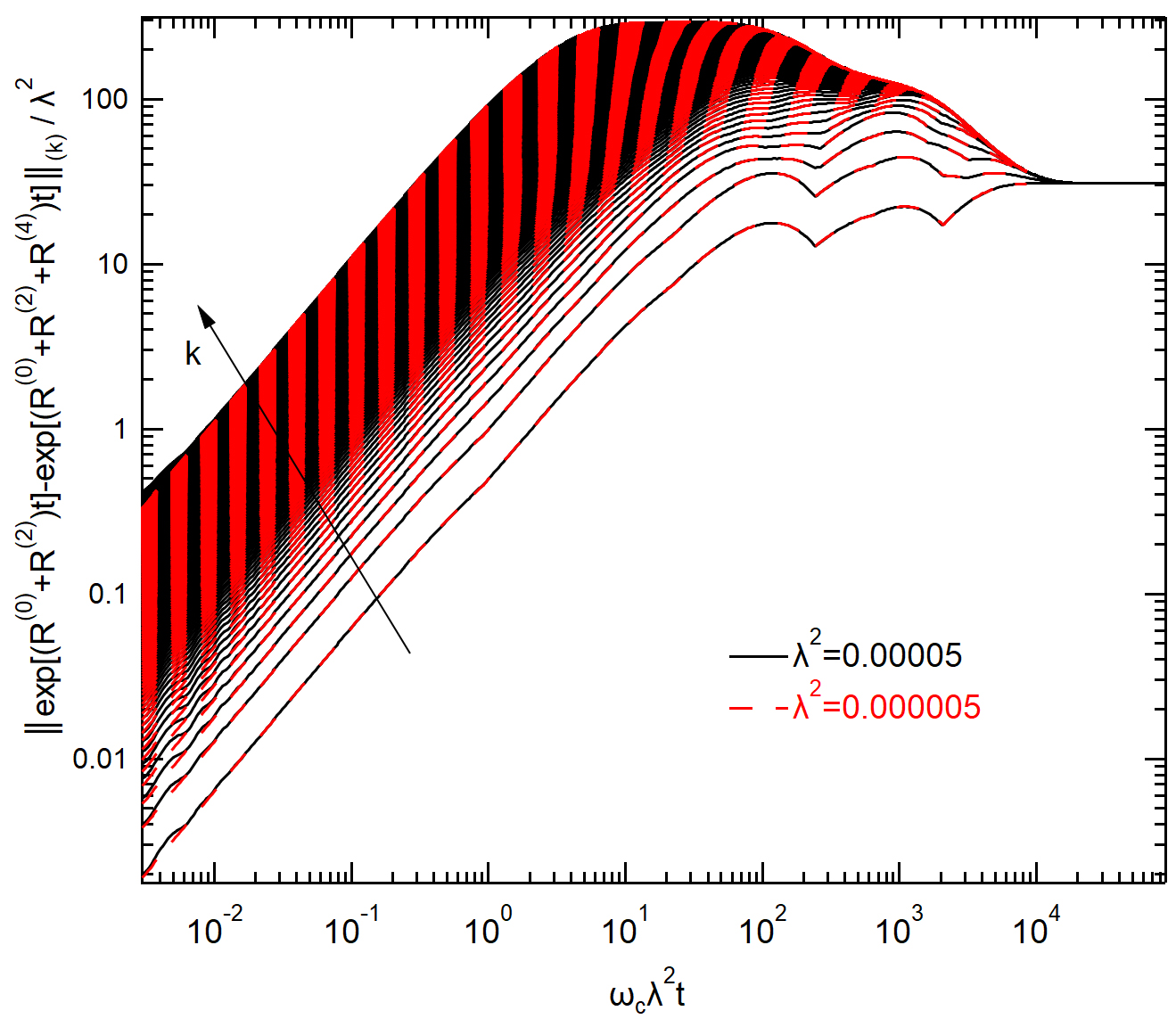
Figure 5: Rescaled Ky Fan norms of the difference between the TCL2 and TCL4 reduced state propagators versus rescaled time. $k=1,2,...,1225$, bottom to top. $N=35$, T=0K, $\omega_{c}=10$, $s=1$.

The significant dispersion in the Ky Fan k-norms over shorter time scales shows that there may be a variety of deviations between the TCL2 and TCL4 dynamics. The crucial issue is that the dynamics’ inaccuracy endures throughout time exceeding the relaxation time $\sim 1/(\lambda^{2}\omega_{c})$. This demonstrates that the Redfield master equation cannot accurately capture the dynamics above the relaxation time. The Davies master equation has the same problem [17].

Appendix F Rayleigh-Schrödinger Perturbation Theory for Fourth-Order Coherences

Here we will derive the Rayleigh-Schrödinger perturbation theory reduced density results seen in Section IV E. As mentioned in the text, we are considering the ground state of $H_{T}=H_{0}+\lambda V$, to be a perturbation of the ground state of $H_{0}=H_{S}+H_{B}$ by the interaction $H_{I}=\lambda V$, where $\lambda$ is a small dimensionless coupling constant. We will expand the ground state $|\tilde{0}\rangle$ and energy $\tilde{\epsilon}_{0}$ of $H_{T}$ in a power series of $\lambda$,

$$|\tilde{0}\rangle = \sum_{k=0}^{\infty}\lambda^{k}|0^{(k)}\rangle,$$ (163)

$$\tilde{\epsilon}_{0} = \sum_{k=0}^{\infty}\lambda^{k}\epsilon^{(k)}.$$ (164)

To zeroth order in $\lambda$, the ground state is that of the free Hamiltonian, $|0^{(0)}\rangle=|0\rangle$ and $\epsilon^{(0)}=\epsilon_{0}$. Since the system and bath are isolated for $H_{0}$, we can express $|0\rangle=|E_{1}\rangle\otimes|\omega_{0}\rangle$ and then $\epsilon_{0}=E_{1}+\omega_{0}$, where $H_{S}|E_{1}\rangle=E_{1}|E_{1}\rangle$ and $H_{B}|\omega_{0}\rangle=\omega_{0}|\omega_{0}\rangle$. We will assume $E_{1}=\omega_{0}=0$.

We will require both our unperturbed and perturbed state to be normalized, that is $\langle 0|0\rangle=\langle\tilde{0}|\tilde{0}\rangle=1$, which gives the condition that at each order $k\geq 1$ we have

$$\sum_{q=0}^{k}\langle 0^{(q)}|0^{(k-q)}\rangle.$$ (165)

We will set $\langle 0|0^{(k)}\rangle=\langle 0^{(k)}|0\rangle$ at each order. Inserting (163) and (164) into the eigenequation $H_{T}|\tilde{0}\rangle=\tilde{\epsilon}_{0}|\tilde{0}\rangle$, and iteratively for the ground state corrections up to fourth order in $\lambda$, we have

$$|0^{(1)}\rangle = \frac{V_{k0}}{d_{0k}}|k\rangle$$ (166)

$$|0^{(2)}\rangle = \frac{V_{kl}V_{l0}}{d_{k0}d_{l0}}|k\rangle-\frac{1}{2}\frac{|V_{0k}|^{2}}{d_{k0}^{2}}|0\rangle$$ (167)

$$|0^{(3)}\rangle = \frac{V_{kl}V_{lm}V_{m0}}{d_{l0}d_{k0}d_{m0}}|k\rangle$$ (168)

$$+ \frac{V_{k0}|V_{l0}|^{2}}{d_{k0}d_{l0}}(\frac{1}{d_{k0}}+\frac{1}{2d_{l0}})|k\rangle$$

$$|0^{(4)}\rangle = \frac{|V_{kl}|^{2}|V_{m0}|^{2}}{d_{k0}d_{m0}d_{kl}^{2}}|k\rangle$$ (169)

$$+ \frac{V_{kl}V_{l0}|V_{m0}|^{2}}{d_{k0}d_{m0}d_{l0}}(\frac{1}{d_{0m}}+\frac{1}{d_{0k}})|k\rangle$$

$$- \frac{V_{kl}V_{lm}V_{mn}V_{n0}}{d_{k0}d_{l0}d_{0m}d_{0n}}|k\rangle$$

$$- \frac{1}{2}\frac{V_{0k}V_{kl}V_{lm}V_{m0}}{d_{k0}d_{l0}d_{m0}}(\frac{1}{d_{l0}}+\frac{1}{d_{m0}})|0\rangle$$

$$- \frac{1}{2}\frac{|V_{0k}|^{2}}{d_{k0}d_{l0}^{2}}(\frac{3}{4}\frac{|V_{0l}|^{2}}{d_{k0}}-\frac{V_{ml}V_{lk}}{d_{m0}})|0\rangle$$

Where we have used notation $V_{nm}=\langle n|V|m\rangle$, $d_{nm}=\epsilon_{n}-\epsilon_{m}$, and each term has a an implicit summation over the eigenbasis of $H_{0}$ for each index, excluding the states that would cause $d_{nn}=0$ factors. We have excluded terms from the perturbative expansion that include $V_{n}n$ terms, as well as terms with $V_{kl}$ where the bath components of the eigenstates would necessarily have the same or an even number difference of bosons, since we have $\langle F\rangle=0$, since our bath coupling operator is linear in bosonic operators. Expanding then the density matrix in orders of $\lambda$, we find

$$\tilde{\rho} = |\tilde{0}\rangle\langle\tilde{0}|=\frac{1}{2}|0\rangle\langle 0|+\lambda|0^{(1)}\rangle\langle 0|+\lambda^{2}|0^{(2)}\rangle\langle 0^{(0)}|$$ (170)

$$+ \frac{\lambda^{2}}{2}|0^{(1)}\rangle\langle 0^{(1)}|)+\lambda^{3}|0^{(2)}\rangle\langle 0^{(1)}|+\lambda^{3}|0^{(3)}\rangle\langle 0^{(0)}|$$

$$+ \frac{\lambda^{4}}{2}|0^{(2)}\rangle\langle 0^{(2)}|+\lambda^{4}|0^{(3)}\rangle\langle 0^{(1)}|$$

$$+ \lambda^{4}|0^{(4)}\rangle\langle 0^{(0)}|+h.c.+O(\lambda^{5}).$$

When calculating $\tilde{\rho}_{S}=\text{Tr}_{B}(\tilde{\rho})$, we see that odd order terms go to zero, again because $\langle F\rangle=0$. Thus we have,

$$\begin{split}\tilde{\rho}_{S}=&\frac{1}{2}|E_{1}\rangle\langle E_{1}|+\lambda^{2}\text{Tr}_{B}(|0^{(2)}\rangle\langle 0^{(0)}|+\frac{1}{2}|0^{(1)}\rangle\langle 0^{(1)}|)\\ +&\lambda^{4}\text{Tr}_{B}(|0^{(4)}\rangle\langle 0^{(0)}|+|0^{(3)}\rangle\langle 0^{(1)}|+\frac{1}{2}|0^{(2)}\rangle\langle 0^{(2)}|)\\ +&h.c.+O(\lambda^{6}).\end{split}$$ (171)

When evaluating these terms, we encounter expressions such as

$$\sum_{\omega_{\alpha}\neq 0}\frac{g_{\alpha}^{2}}{(w+\omega_{\alpha})}=\int_{-\infty}^{\infty}d\omega\sum_{\omega_{\alpha}\neq 0}\frac{g_{\alpha}^{2}\delta(\omega-\omega_{\alpha})}{(w+\omega_{\alpha})}\\ =-\int_{-\infty}^{\infty}d\omega\sum_{\omega_{\alpha}\neq 0}\frac{g_{\alpha}^{2}\delta(\omega-\omega_{\alpha})}{[(-w)-\omega_{\alpha}]}=-\tilde{\mathcal{S}}_{-w}$$ (172)

for $-w\neq\omega_{\alpha}$, which will always be the case due to our limitation of only nonzero $d_{mn}$.

Similarly, we will encounter,

$$\sum_{\omega_{\alpha}\neq 0}\frac{g_{\alpha}^{2}}{(w+\omega_{\alpha})^{2}}=-\partial\tilde{\mathcal{S}}_{-w}$$ (173)

Looking at just at the second order terms from (171), tracing over the bath degrees of freedom we find

$$\begin{split}\tilde{\rho}_{S}^{(2)}=&\lambda^{2}\text{Tr}_{B}(|0^{(2)}\rangle\langle 0^{(0)}|+|0^{(0)}\rangle\langle 0^{(2)}|+\frac{1}{2}|0^{(1)}\rangle\langle 0^{(1)}|)=\sum_{\begin{subarray}{c}n=2\\ k=1\end{subarray}}^{N}\sum_{\alpha}\frac{A_{nk}A_{k1}g_{\alpha}^{2}}{E_{n}(E_{k}+\omega_{\alpha})}|E_{n}\rangle\langle E_{1}|\\ &+\frac{1}{2}\sum_{n,m=1}^{N}\sum_{\alpha}\frac{A_{n1}A_{1m}g_{\alpha}^{2}}{(E_{n}+\omega_{\alpha})(E_{m}+\omega_{\alpha})}|E_{n}\rangle\langle E_{m}|-\frac{1}{2}\sum_{n=1}^{N}\sum_{\alpha}\frac{|A_{1n}|^{2}g_{\alpha}^{2}}{(E_{n}+\omega_{\alpha})^{2}}|E_{1}\rangle\langle E_{1}|+h.c.\end{split}$$ (174)

Note, we have used the Eq. 6 definition of the bath coupling operator $F$ when tracing over the bath (all Fock space eigenstates), we find

$$\sum_{\omega_{k}\neq 0}|F_{0k}|^{2}=\langle 0|F|\omega_{k}\rangle\langle\omega_{k}|F|0\rangle=\sum_{\alpha}g_{\alpha}^{2}$$ (175)

That is, for these terms the only nonzero contribution is from the single-particle states, and we can express these products in terms of the form factors.

It should be noted that the last term in the (174) results from the normalization of $|\tilde{0}\rangle$ giving a second order condition that $\langle 0|0^{(2)}\rangle=-\frac{1}{2}\langle 0^{(1)}|0^{(1)}\rangle$. We will see that this term cancels a possible divergence in the populations. If we instead required the perturbations be orthogonal to the isolated state, $\langle 0|0^{(k)}\rangle=0\forall k>0$, at second order in alpha we would have a $\frac{\partial S(-E_{1})}{\partial E_{1}}$ diverging term, in the case when $a=b=1$.

We will now relate our second order term to our continuum limit spectral densities, using (172) and (173), we have

$$\begin{split}\tilde{\rho}_{S}^{(2)}=-\sum_{\begin{subarray}{c}a=2\\ b=2\end{subarray}}^{N}\frac{\mathcal{S}_{{1b}}}{\omega_{a1}}(A_{ab}A_{b1}|E_{a}\rangle\langle E_{1}|+A_{1b}A_{ba}|E_{1}\rangle\langle E_{a}|)\\ +\sum_{\begin{subarray}{c}a,b=2\\ a\not=b\end{subarray}}^{N}A_{a1}A_{1b}\frac{(\mathcal{S}_{{1a}}-\mathcal{S}_{{1b}})}{\omega_{ab}}|E_{a}\rangle\langle E_{b}|+\sum_{a=2}^{N}|A_{1a}|^{2}\mathcal{\partial}{S}_{{1a}}(|E_{a}\rangle\langle E_{a}|-|E_{1}\rangle\langle E_{1}|).\end{split}$$ (176)

Leading to equations 78 and 79 in the main text. Using this same approach for the $O(\lambda^{4})$ terms, we find

$$\tilde{\rho}^{(4)} = |n\rangle\langle m|[\frac{(V_{nl}V_{l0}V_{km}V_{0k}-V_{nl}V_{lk}V_{0m}V_{k0}-V_{n0}V_{kl}V_{lm}V_{0k})}{d_{l0}d_{k0}d_{m0}d_{n0}}-\frac{V_{n0}V_{0m}|V_{k0}|^{2}}{d_{n0}d_{m0}d_{k0}}(\frac{1}{d_{n0}}+\frac{1}{d_{k0}}+\frac{1}{d_{m0}})]$$ (177)

$$+ |0\rangle\langle 0|[\frac{1}{2}\frac{|V_{0k}|^{2}(V_{kl}V_{lm}+V_{ml}V_{lk})}{d_{m0}d_{k0}d_{l0}^{2}}-\frac{1}{2}\frac{|V_{0k}|^{2}|V_{0l}|^{2}}{d_{k0}^{2}d_{l0}^{2}}-\frac{1}{2}\frac{V_{k0}V_{lk}V_{ml}V_{0m}}{d_{m0}d_{l0}d_{k0}}(\frac{1}{d_{m0}}+\frac{1}{d_{k0}}+\frac{2}{d_{l0}})]$$ (178)

$$+ |n\rangle\langle 0|[\frac{|V_{nl}|^{2}|V_{k0}|^{2}}{d_{n0}d_{k0}d_{nl}^{2}}-\frac{V_{nl}V_{lm}V_{mk}V_{k0}}{d_{n0}d_{l0}d_{m0}d_{k0}}-\frac{V_{nl}V_{l0}|V_{k0}|^{2}}{d_{n0}d_{k0}d_{l0}}(\frac{3}{2d_{k0}}+\frac{1}{d_{n0}})]$$ (179)

$$+ |0\rangle\langle m|[\frac{|V_{ml}|^{2}|V_{k0}|^{2}}{d_{m0}d_{k0}d_{ml}^{2}}-\frac{V_{lm}V_{kl}V_{nk}V_{0n}}{d_{m0}d_{l0}d_{k0}d_{n0}}-\frac{|V_{k0}|^{2}V_{lm}V_{0l}}{d_{m0}d_{k0}d_{l0}}(\frac{3}{2d_{k0}}+\frac{1}{d_{m0}})].$$ (180)

Tracing over the bath degrees of freedom, we will use the notation introduced in (175) as well as a new definition $D_{ka}=E_{k}+\omega_{a}$, assigning indices to the system and bath part of the total energy eigenvalues, i.e. $|\epsilon_{i}\rangle=|E_{k}\rangle\otimes|\omega_{a}\rangle$ to find

$$\tilde{\rho}_{S}^{(4)} = A_{nl}A_{l1}A_{km}A_{1k}\frac{|F_{0a}|^{2}|F_{b0}|^{2}}{E_{m}E_{n}D_{la}D_{kb}}|E_{n}\rangle\langle E_{m}|+A_{nl}A_{l1}A_{km}A_{1k}\frac{F_{ca}F_{a0}F_{bc}F_{0b}}{D_{nc}D_{ma}D_{kb}D_{la}}|E_{n}\rangle\langle E_{m}|$$

$$- (A_{nl}A_{lk}A_{1m}A_{k1}+A_{n1}A_{kl}A_{lm}A_{1k})\frac{|F_{0a}|^{2}|F_{0b}|^{2}}{E_{l}D_{na}D_{ma}D_{kb}}|E_{n}\rangle\langle E_{m}|$$

$$- (A_{nl}A_{lk}A_{1m}A_{k1}\frac{F_{ac}F_{cb}F_{0a}F_{b0}}{D_{na}D_{ma}D_{kb}D_{lc}}+A_{n1}A_{kl}A_{lm}A_{1k}\frac{F_{bc}F_{ca}F_{a0}F_{0b}}{D_{na}D_{ma}D_{kb}D_{lc}})|E_{n}\rangle\langle E_{m}|$$

$$- A_{n1}A_{1m}|A_{k1}|^{2}\frac{|F_{a0}|^{2}|F_{b0}|^{2}}{D_{kb}D_{na}D_{ma}}(\frac{1}{D_{na}}+\frac{1}{D_{kb}}+\frac{1}{D_{ma}})|E_{n}\rangle\langle E_{m}|$$

$$+ \frac{|A_{1k}|^{2}|F_{0b}|^{2}}{D_{ma}D_{kb}}[\frac{\text{Re}(A_{kl}A_{lm}F_{bc}F_{ca})}{D_{lc}^{2}}+\frac{\text{Re}(A_{kl}A_{lm}F_{b0}F_{0a})}{E_{l}}]|E_{1}\rangle\langle E_{1}|$$

$$- \frac{1}{2}A_{k1}A_{lk}A_{ml}A_{1m}\frac{|F_{0a}|^{2}|F_{0b}|^{2}}{E_{l}D_{ma}D_{kb}}(\frac{1}{D_{ma}}+\frac{1}{D_{kb}}+\frac{2}{E_{l}})|E_{1}\rangle\langle E_{1}|-\frac{1}{2}|A_{1k}|^{2}|A_{1l}|^{2}\frac{|F_{0a}|^{2}|F_{0b}|^{2}}{D_{kb}^{2}D_{la}^{2}}|E_{1}\rangle\langle E_{1}|$$

$$- \frac{1}{2}A_{k1}A_{lk}A_{ml}A_{1m}\frac{F_{b0}F_{ac}F_{cb}F_{0a}}{D_{ma}D_{kb}D_{lc}}(\frac{1}{D_{ma}}+\frac{1}{D_{kb}}+\frac{2}{D_{lc}})|E_{1}\rangle\langle E_{1}|$$

$$+ |A_{ml}|^{2}|A_{k1}|^{2}\frac{|F_{0a}|^{2}|F_{b0}|^{2}}{E_{m}D_{kb}(w_{ml}-\omega_{a})^{2}}|E_{1}\rangle\langle E_{m}|-A_{lm}A_{kl}A_{nk}A_{1n}\frac{|F_{0a}|^{2}|F_{0b}|^{2}}{E_{m}E_{k}D_{la}D_{nb}}|E_{1}\rangle\langle E_{m}|$$

$$- |A_{k1}|^{2}A_{lm}A_{1l}\frac{|F_{0b}|^{2}|F_{0a}|^{2}}{E_{m}D_{kb}D_{la}}(\frac{3}{2D_{kb}}+\frac{1}{E_{m}})|E_{1}\rangle\langle E_{m}|-A_{lm}A_{kl}A_{nk}A_{1n}\frac{F_{a0}F_{bc}F_{ca}F_{0b}}{E_{m}D_{la}D_{kc}D_{nb}}|E_{1}\rangle\langle E_{m}|$$

$$+ (|E_{n}\rangle\langle E_{1}|\text{ terms})$$

Where the $|E_{n}\rangle\langle E_{1}|$ terms are the hermitian conjugate of the $|E_{1}\rangle\langle E_{m}|$ expressions, with the additional change of $m\leftrightarrow n$. There are implicit summations for each index, and it should be noted that each bath energy index (e.g. $a,b,c$), represents a sum over the occupied states only, as the nonzero terms from an index being the vacuum state have been separated off. To evaluate these terms, plugging the bosonic operators in as in (175), we find

$$\sum_{a,b,c}\frac{F_{a0}F_{ca}F_{bc}F_{b0}}{D_{la}D_{kb}D_{ic}} = \sum_{a,b}\frac{g_{a}^{2}g_{b}^{2}}{D_{la}(E_{i}+\omega_{a}+\omega_{b})}\left(\frac{1}{D_{ka}}+\frac{1}{D_{kb}}\right)$$ (182)

$$= \sum_{a,b}\left[\frac{g_{b}^{2}}{(E_{i}+\omega_{a}+\omega_{b})}\left(\frac{g_{a}^{2}}{D_{ka}D_{la}}-\frac{g_{a}^{2}}{(\omega_{ik}+\omega_{a})D_{la}}\right)+\frac{g_{a}^{2}}{(\omega_{ik}+\omega_{a})D_{la}}\frac{g_{b}^{2}}{D_{kb}}\right].$$

We consider the case $\tilde{\rho}_{S,nm}^{(4)}$ with $n\neq m$ and $n,m=2,\ldots,N$, applying  (182), after some algebra we find

$$\tilde{\rho}^{(4)}_{S,nm} = A_{nl}A_{l1}A_{km}A_{1k}\frac{g_{a}^{2}g_{b}^{2}}{E_{m}E_{n}D_{la}D_{kb}}$$ (183)

$$- A_{n1}A_{1m}|A_{k1}|^{2}\left[\frac{g_{b}^{2}}{\omega_{nm}D_{kb}}(\frac{g_{a}^{2}}{D_{ma}^{2}}-\frac{g_{a}^{2}}{D_{na}^{2}})+\frac{g_{b}^{2}}{\omega_{nm}D_{kb}^{2}}\left(\frac{g_{a}^{2}}{D_{ma}}-\frac{g_{a}^{2}}{D_{na}}\right)\right]$$

$$+ (A_{nl}A_{lk}A_{1m}A_{k1}+A_{n1}A_{kl}A_{lm}A_{1k})\frac{1}{\omega_{nm}}\frac{g_{b}^{2}}{D_{kb}}$$

$$\times \left[\frac{g_{a}^{2}}{D_{na}(\omega_{lk}+\omega_{a})}-\frac{g_{a}^{2}}{D_{ma}(\omega_{lk}+\omega_{a})}-\frac{g_{a}^{2}}{E_{l}D_{na}}+\frac{g_{a}^{2}}{E_{l}D_{ma}}\right]$$

$$+ A_{nl}A_{l1}A_{km}A_{1k}\frac{1}{\omega_{nm}}\frac{g_{b}^{2}}{D_{kb}}\left[\frac{g_{a}^{2}}{D_{la}(\omega_{mk}+\omega_{a})}-\frac{g_{a}^{2}}{D_{la}(\omega_{nk}+\omega_{a})}\right]$$

$$+ A_{nl}A_{l1}A_{km}A_{1k}\frac{1}{\omega_{nm}}\frac{g_{b}^{2}}{(E_{m}+\omega_{a}+\omega_{b})}\left[\frac{g_{a}^{2}}{D_{la}D_{ka}}-\frac{g_{a}^{2}}{D_{la}(\omega_{mk}+\omega_{a})}\right]$$

$$- A_{nl}A_{l1}A_{km}A_{1k}\frac{1}{\omega_{nm}}\frac{g_{b}^{2}}{(E_{n}+\omega_{a}+\omega_{b})}\left[\frac{g_{a}^{2}}{D_{la}D_{ka}}-\frac{g_{a}^{2}}{D_{la}(\omega_{nk}+\omega_{a})}\right]$$

$$+ (A_{nl}A_{lk}A_{1m}A_{k1}+A_{n1}A_{kl}A_{lm}A_{1k})\frac{1}{\omega_{nm}}\frac{g_{b}^{2}}{(E_{l}+\omega_{a}+\omega_{b})}\left(\frac{g_{a}^{2}}{D_{na}D_{ka}}-\frac{g_{a}^{2}}{D_{ma}D_{ka}}\right)$$

$$- (A_{nl}A_{lk}A_{1m}A_{k1}+A_{n1}A_{kl}A_{lm}A_{1k})\frac{1}{\omega_{nm}}\frac{g_{b}^{2}}{(E_{l}+\omega_{a}+\omega_{b})}\left(\frac{g_{a}^{2}}{D_{na}(\omega_{lk}+\omega_{a})}-\frac{g_{a}^{2}}{D_{ma}(\omega_{lk}+\omega_{a})}\right),$$

with summations over all the indices (excluding $n,m$) still implicit. We then map from the discrete frequencies to a continuous distribution using Eqs. (172),(173)

and the general mapping

$$\sum_{a}g_{a}^{2}f(\omega_{a})\mapsto\int_{-\infty}^{\infty}\frac{d\omega}{\pi}\tilde{\mathcal{J}}_{\omega}f(\omega),$$ (184)

with $f(\omega_{a})$ a function describing the dependence of $\omega_{a}$ within each term. This gives Eq. 79. Evaluating the other coherence terms in Eqn. (F), $\tilde{\rho}_{S,1m}^{(4)}$ with $m=2,\ldots,N$, we find

$$\tilde{\rho}_{S,1m}^{(4)} = A_{1l}A_{l1}A_{km}A_{1k}\frac{g_{a}^{2}}{(\omega_{1k}+\omega_{a})D_{la}}\left[\frac{g_{b}^{2}}{E_{m}D_{kb}}-\frac{g_{b}^{2}}{E_{m}(\omega_{a}+\omega_{b})}\right]$$ (185)

$$- A_{1l}A_{l1}A_{km}A_{1k}\frac{g_{a}^{2}}{(\omega_{mk}+\omega_{a})D_{la}}\left[\frac{g_{b}^{2}}{E_{m}D_{kb}}-\frac{g_{b}^{2}}{E_{m}(E_{m}+\omega_{a}+\omega_{b})}\right]$$

$$- A_{pm}A_{lp}A_{kl}A_{1k}\frac{g_{a}^{2}}{(\omega_{lk}+\omega_{a})D_{pa}}\left[\frac{g_{b}^{2}}{E_{m}D_{kb}}-\frac{g_{b}^{2}}{E_{m}(E_{l}+\omega_{a}+\omega_{b})}\right]$$

$$+ \left(A_{1l}A_{lk}A_{1m}A_{k1}+A_{11}A_{kl}A_{lm}A_{1k}\right)\frac{g_{a}^{2}}{(\omega_{lk}+\omega_{a})D_{ma}}\left[\frac{g_{b}^{2}}{E_{m}D_{kb}}-\frac{g_{b}^{2}}{E_{m}(E_{l}+\omega_{a}+\omega_{b})}\right]$$

$$- \left(A_{1l}A_{lk}A_{1m}A_{k1}+A_{11}A_{kl}A_{lm}A_{1k}\right)\frac{g_{a}^{2}}{(\omega_{lk}+\omega_{a})D_{1a}}\left[\frac{g_{b}^{2}}{E_{m}D_{kb}}-\frac{g_{b}^{2}}{E_{m}(E_{l}+\omega_{a}+\omega_{b})}\right]$$

$$+ \left(A_{1l}A_{lk}A_{1m}A_{k1}+A_{11}A_{kl}A_{lm}A_{1k}\right)\frac{g_{b}^{2}}{E_{m}(E_{l}+\omega_{a}+\omega_{b})}\left(\frac{g_{a}^{2}}{D_{ma}D_{ka}}-\frac{g_{a}^{2}}{D_{1a}D_{ka}}\right)$$

$$+ A_{1l}A_{l1}A_{km}A_{1k}\frac{g_{a}^{2}}{D_{ka}D_{la}}\left[\frac{g_{b}^{2}}{E_{m}(\omega_{a}+\omega_{b})}-\frac{g_{b}^{2}}{E_{m}(E_{m}+\omega_{a}+\omega_{b})}\right]$$

$$- A_{pm}A_{lp}A_{kl}A_{1k}\frac{g_{a}^{2}}{D_{ka}D_{pa}}\left[\frac{g_{b}^{2}}{E_{m}(E_{l}+\omega_{a}+\omega_{b})}\right]-\frac{3}{2}A_{1l}A_{lm}|A_{k1}|^{2}\frac{g_{a}^{2}}{D_{ka}^{2}}\frac{g_{b}^{2}}{E_{m}D_{lb}}$$

$$- A_{11}A_{1m}|A_{k1}|^{2}\frac{g_{a}^{2}}{D_{ka}^{2}}\left(\frac{g_{b}^{2}}{E_{m}D_{1b}}-\frac{g_{b}^{2}}{E_{m}D_{mb}}\right)+|A_{ml}|^{2}|A_{k1}|^{2}\frac{g_{a}^{2}}{(\omega_{ml}-\omega_{a})^{2}}\frac{g_{b}^{2}}{E_{m}D_{kb}}$$

$$- A_{11}A_{1m}|A_{k1}|^{2}\frac{g_{a}^{2}}{D_{1a}^{2}}\frac{g_{b}^{2}}{E_{m}D_{kb}}-(A_{1m}A_{mk}A_{1l}A_{k1}+A_{11}A_{km}A_{ml}A_{1k})\frac{g_{a}^{2}}{D_{1a}D_{la}}\frac{g_{b}^{2}}{E_{m}D_{kb}}$$

$$- \left(A_{km}A_{pk}A_{lp}A_{1l}\frac{1}{E_{p}}+A_{1l}A_{lm}|A_{k1}|^{2}\frac{1}{E_{m}}\right)\frac{g_{b}^{2}}{E_{m}D_{lb}}\frac{g_{a}^{2}}{D_{ka}}+A_{11}A_{1m}|A_{k1}|^{2}\frac{g_{a}^{2}}{D_{ma}^{2}}\frac{g_{b}^{2}}{E_{m}D_{kb}},$$

where the summations over open system indices are still implicit.

References

- Fröhlich and Schubnel [2016] J. Fröhlich and B. Schubnel, The preparation of states in quantum mechanics, Journal of Mathematical Physics 57 (2016).
- Engel et al. [2007] G. S. Engel, T. R. Calhoun, E. L. Read, T.-K. Ahn, T. Mančal, Y.-C. Cheng, R. E. Blankenship, and G. R. Fleming, Evidence for wavelike energy transfer through quantum coherence in photosynthetic systems, Nature 446, 782 (2007).
- Carleo et al. [2012] G. Carleo, F. Becca, M. Schiró, and M. Fabrizio, Localization and glassy dynamics of many-body quantum systems, Scientific reports 2, 243 (2012).
- Shandera et al. [2018] S. Shandera, N. Agarwal, and A. Kamal, Open quantum cosmological system, Physical Review D 98, 083535 (2018).
- Collini and Scholes [2009] E. Collini and G. D. Scholes, Coherent intrachain energy migration in a conjugated polymer at room temperature, science 323, 369 (2009).
- Zurek [2009] W. H. Zurek, Quantum darwinism, Nature physics 5, 181 (2009).
- Feynman and Vernon [1963] R. Feynman and F. Vernon, The theory of a general quantum system interacting with a linear dissipative system, Annals of Physics 24, 118 (1963).
- Meyer et al. [1990] H.-D. Meyer, U. Manthe, and L. S. Cederbaum, The multi-configurational time-dependent hartree approach, Chemical Physics Letters 165, 73 (1990).
- Strathearn et al. [2018] A. Strathearn, P. Kirton, D. Kilda, J. Keeling, and B. W. Lovett, Efficient non-Markovian quantum dynamics using time-evolving matrix product operators, Nat. Commun. 9, 3322 (2018).
- Makri [2020] N. Makri, Small matrix disentanglement of the path integral: overcoming the exponential tensor scaling with memory length, The Journal of Chemical Physics 152 (2020).
- Tanimura and Kubo [1989] Y. Tanimura and R. Kubo, Time evolution of a quantum system in contact with a nearly gaussian-markoffian noise bath, Journal of the Physical Society of Japan 58, 101 (1989).
- REDFIELD [1965] A. REDFIELD, The theory of relaxation processes* *this work was started while the author was at harvard university, and was then partially supported by joint services contract n5ori-76, project order i., in Advances in Magnetic Resonance, Advances in Magnetic and Optical Resonance, Vol. 1, edited by J. S. Waugh (Academic Press, 1965) pp. 1 – 32.
- Liu et al. [2018] Y.-y. Liu, Y.-m. Yan, M. Xu, K. Song, and Q. Shi, Exact generator and its high order expansions in time-convolutionless generalized master equation: Applications to spin-boson model and excitation energy transfer, Chinese Journal of Chemical Physics 31, 575 (2018).
- Becker et al. [2022] T. Becker, A. Schnell, and J. Thingna, Canonically consistent quantum master equation, Physical Review Letters 129, 200403 (2022).
- Fleming and Cummings [2011] C. H. Fleming and N. I. Cummings, Accuracy of perturbative master equations, Phys. Rev. E 83, 031117 (2011).
- Tupkary et al. [2021] D. Tupkary, A. Dhar, M. Kulkarni, and A. Purkayastha, Fundamental limitations in lindblad descriptions of systems weakly coupled to baths (2021), arXiv:2105.12091 [quant-ph] .
- Davies [1974] E. B. Davies, Markovian master equations, Comm. Math. Phys. 39, 91 (1974).
- Schaller and Brandes [2008] G. Schaller and T. Brandes, Preservation of positivity by dynamical coarse graining, Phys. Rev. A 78, 022106 (2008).
- Benatti et al. [2010] F. Benatti, R. Floreanini, and U. Marzolino, Entangling two unequal atoms through a common bath, Phys. Rev. A 81, 012105 (2010).
- Benatti et al. [2009] F. Benatti, R. Floreanini, and U. Marzolino, Environment-induced entanglement in a refined weak-coupling limit, EPL (Europhysics Letters) 88, 20011 (2009).
- Majenz et al. [2013] C. Majenz, T. Albash, H.-P. Breuer, and D. A. Lidar, Coarse graining can beat the rotating-wave approximation in quantum markovian master equations, Phys. Rev. A 88, 012103 (2013).
- Cresser and Facer [2017] J. D. Cresser and C. Facer, Coarse-graining in the derivation of markovian master equations and its significance in quantum thermodynamics (2017), arXiv:1710.09939 [quant-ph] .
- Farina and Giovannetti [2019] D. Farina and V. Giovannetti, Open-quantum-system dynamics: Recovering positivity of the redfield equation via the partial secular approximation, Phys. Rev. A 100, 012107 (2019).
- Hartmann and Strunz [2020] R. Hartmann and W. T. Strunz, Accuracy assessment of perturbative master equations: Embracing nonpositivity, Phys. Rev. A 101, 012103 (2020).
- Mozgunov and Lidar [2020] E. Mozgunov and D. Lidar, Completely positive master equation for arbitrary driving and small level spacing, 4, 227 (2020), 1908.01095 [Quantum] .
- Vogt et al. [2013] N. Vogt, J. Jeske, and J. H. Cole, Stochastic bloch-redfield theory: Quantum jumps in a solid-state environment, Phys. Rev. B 88, 174514 (2013).
- Tscherbul and Brumer [2015] T. V. Tscherbul and P. Brumer, Partial secular bloch-redfield master equation for incoherent excitation of multilevel quantum systems, The Journal of Chemical Physics 142, 104107 (2015), https://doi.org/10.1063/1.4908130 .
- Trushechkin [2021a] A. Trushechkin, Unified gorini-kossakowski-lindblad-sudarshan quantum master equation beyond the secular approximation, Phys. Rev. A 103, 062226 (2021a).
- Gerry and Segal [2023] M. Gerry and D. Segal, Full counting statistics and coherences: Fluctuation symmetry in heat transport with the unified quantum master equation, Physical Review E 107, 054115 (2023).
- Palmieri et al. [2009] B. Palmieri, D. Abramavicius, and S. Mukamel, Lindblad equations for strongly coupled populations and coherences in photosynthetic complexes, The Journal of Chemical Physics 130, 204512 (2009), https://doi.org/10.1063/1.3142485 .
- Kiršanskas et al. [2018] G. Kiršanskas, M. Franckié, and A. Wacker, Phenomenological position and energy resolving lindblad approach to quantum kinetics, Phys. Rev. B 97, 035432 (2018).
- Ptaszyński and Esposito [2019] K. Ptaszyński and M. Esposito, Thermodynamics of quantum information flows, Phys. Rev. Lett. 122, 150603 (2019).
- Kleinherbers et al. [2020] E. Kleinherbers, N. Szpak, J. König, and R. Schützhold, Relaxation dynamics in a hubbard dimer coupled to fermionic baths: Phenomenological description and its microscopic foundation, Phys. Rev. B 101, 125131 (2020).
- Davidović [2020] D. Davidović, Completely positive, simple, and possibly highly accurate approximation of the redfield equation, Quantum 4, 326 (2020).
- Nathan and Rudner [2020] F. Nathan and M. S. Rudner, Universal lindblad equation for open quantum systems, Phys. Rev. B 102, 115109 (2020).
- Merkli [2020] M. Merkli, Quantum markovian master equations: Resonance theory shows validity for all time scales, Annals of Physics 412, 167996 (2020).
- Merkli [2022a] M. Merkli, Dynamics of open quantum systems i, oscillation and decay, Quantum 6, 615 (2022a).
- Merkli [2022b] M. Merkli, Dynamics of open quantum systems ii, markovian approximation, Quantum 6, 616 (2022b).
- Albash et al. [2012] T. Albash, S. Boixo, D. A. Lidar, and P. Zanardi, Quantum adiabatic markovian master equations, New Journal of Physics 14, 123016 (2012).
- Becker et al. [2021] T. Becker, L.-N. Wu, and A. Eckardt, Lindbladian approximation beyond ultraweak coupling, Phys. Rev. E 104, 014110 (2021).
- Rivas [2017] A. Rivas, Refined weak-coupling limit: Coherence, entanglement, and non-markovianity, Phys. Rev. A 95, 042104 (2017).
- Winczewski et al. [2021] M. Winczewski, A. Mandarino, M. Horodecki, and R. Alicki, Bypassing the intermediate times dilemma for open quantum system (2021), arXiv:2106.05776 [quant-ph] .
- D’Abbruzzo et al. [2023] A. D’Abbruzzo, V. Cavina, and V. Giovannetti, A time-dependent regularization of the redfield equation, SciPost Physics 15, 117 (2023).
- Potts et al. [2021] P. P. Potts, A. A. S. Kalaee, and A. Wacker, A thermodynamically consistent markovian master equation beyond the secular approximation, New Journal of Physics 23, 123013 (2021).
- Tupkary et al. [2023] D. Tupkary, A. Dhar, M. Kulkarni, and A. Purkayastha, Searching for lindbladians obeying local conservation laws and showing thermalization, arXiv preprint arXiv:2301.02146 (2023).
- Uchiyama [2023] C. Uchiyama, Dynamics of a quantum interacting system-extended global approach beyond the born-markov and secular approximation, arXiv preprint arXiv:2303.02926 (2023).
- Winczewski and Alicki [2021] M. Winczewski and R. Alicki, Renormalization in the theory of open quantum systems via the self-consistency condition, arXiv preprint arXiv:2112.11962 (2021).
- Tokuyama and Mori [1976] M. Tokuyama and H. Mori, Statistical-mechanical theory of the boltzmann equation and fluctuations in space, Progress of Theoretical Physics 56, 1073 (1976).
- Yoon et al. [2008] B. Yoon, J. M. Deutch, and J. H. Freed, A comparison of generalized cumulant and projection operator methods in spin-relaxation theory, The Journal of Chemical Physics 62, 4687 (2008), https://pubs.aip.org/aip/jcp/article-pdf/62/12/4687/11157754/4687_1_online.pdf .
- Mukamel et al. [1978] S. Mukamel, I. Oppenheim, and J. Ross, Statistical reduction for strongly driven simple quantum systems, Phys. Rev. A 17, 1988 (1978).
- Shibata et al. [1977] F. Shibata, Y. Takahashi, and N. Hashitsume, A generalized stochastic liouville equation. non-markovian versus memoryless master equations, Journal of Statistical Physics 17, 171 (1977).
- Shibata and Arimitsu [1980] F. Shibata and T. Arimitsu, Expansion formulas in nonequilibrium statistical mechanics, Journal of the Physical Society of Japan 49, 891 (1980).
- Laird et al. [1991] B. B. Laird, J. Budimir, and J. L. Skinner, Quantum-mechanical derivation of the bloch equations: Beyond the weak-coupling limit, The Journal of chemical physics 94, 4391 (1991).
- Reichman et al. [1997] D. R. Reichman, F. L. H. Brown, and P. Neu, Cumulant expansions and the spin-boson problem, Phys. Rev. E 55, 2328 (1997).
- Breuer et al. [1999] H.-P. Breuer, B. Kappler, and F. Petruccione, Stochastic wave-function method for non-markovian quantum master equations, Physical Review A 59, 1633–1643 (1999).
- Jang et al. [2002] S. Jang, J. Cao, and R. J. Silbey, Fourth-order quantum master equation and its markovian bath limit, The Journal of Chemical Physics 116, 2705 (2002), https://doi.org/10.1063/1.1445105 .
- Trushechkin [2019] A. Trushechkin, Higher-order corrections to the redfield equation with respect to the system-bath coupling based on the hierarchical equations of motion, Lobachevskii Journal of Mathematics 40, 1606 (2019).
- Trushechkin [2021b] A. S. Trushechkin, Derivation of the redfield quantum master equation and corrections to it by the bogoliubov method, Proceedings of the Steklov Institute of Mathematics 313, 246 (2021b).
- Nestmann and Timm [2019] K. Nestmann and C. Timm, Time-convolutionless master equation: Perturbative expansions to arbitrary order and application to quantum dots (2019), arXiv:1903.05132 [cond-mat.mes-hall] .
- Karasev and Teretenkov [2023] A. Y. Karasev and A. E. Teretenkov, Time-convolutionless master equations for composite open quantum systems (2023), arXiv:2304.08627 [quant-ph] .
- Araki and Woods [1963] H. Araki and E. Woods, Representations of the canonical commutation relations describing a nonrelativistic infinite free bose gas, Journal of Mathematical Physics 4, 637 (1963).
- Merkli [2006] M. Merkli, The ideal quantum gas, in Open Quantum Systems I: The Hamiltonian Approach (Springer, 2006) pp. 183–233.
- Spohn [1989] H. Spohn, Ground state (s) of the spin-boson hamiltonian, Communications in mathematical physics 123, 277 (1989).
- De Roeck and Kupiainen [2013] W. De Roeck and A. Kupiainen, Approach to ground state and time-independent photon bound for massless spin-boson models, in Annales Henri Poincaré, Vol. 14 (Springer, 2013) pp. 253–311.
- Dereziński and Gérard [2004] J. Dereziński and C. Gérard, Scattering theory of infrared divergent pauli-fierz hamiltonians, in Annales Henri Poincaré, Vol. 5 (Springer, 2004) pp. 523–577.
- Jakšić and Pillet [1996] V. Jakšić and C.-A. Pillet, On a model for quantum friction iii. ergodic properties of the spin-boson system, Communications in Mathematical Physics 178, 627 (1996).
- Bach et al. [2000] V. Bach, J. Fröhlich, and I. M. Sigal, Return to equilibrium, Journal of Mathematical Physics 41, 3985 (2000).
- Weiss [2012] U. Weiss, Quantum Dissipative Systems, 4th ed. (WORLD SCIENTIFIC, 2012) https://www.worldscientific.com/doi/pdf/10.1142/8334 .
- Nemati et al. [2022] S. Nemati, C. Henkel, and J. Anders, Coupling function from bath density of states, Europhysics Letters 139, 36002 (2022).
- Breuer and Petruccione [2007] H.-P. Breuer and F. Petruccione, The theory of open quantum systems (2007).
- Faupin and Sigal [2014] J. Faupin and I. M. Sigal, On rayleigh scattering in non-relativistic quantum electrodynamics, Communications in Mathematical Physics 328, 1199 (2014).
- De Roeck et al. [2015] W. De Roeck, M. Griesemer, and A. Kupiainen, Asymptotic completeness for the massless spin-boson model, Advances in Mathematics 268, 62 (2015).
- Arai and Hirokawa [1997] A. Arai and M. Hirokawa, On the existence and uniqueness of ground states of a generalized spin-boson model, journal of functional analysis 151, 455 (1997).
- Bach et al. [1999] V. Bach, J. Fröhlich, and I. M. Sigal, Spectral analysis for systems of atoms and molecules coupled to the quantized radiation field, Communications in Mathematical Physics 207, 249 (1999).
- Gerard [2000] C. Gerard, On the existence of ground states for massless pauli-fierz hamiltonians, Annales Henri Poincar 1, 443 (2000).
- Griesemer et al. [2001] M. Griesemer, E. H. Lieb, and M. Loss, Ground states in non-relativistic quantum electrodynamics, Inventiones mathematicae 145, 557 (2001).
- Hasler and Herbst [2011] D. Hasler and I. Herbst, Ground states in the spin boson model, in Annales Henri Poincaré, Vol. 12 (Springer, 2011) pp. 621–677.
- Abdesselam [2011] A. Abdesselam, The ground state energy of the massless spin-boson model, in Annales Henri Poincaré, Vol. 12 (Springer, 2011) pp. 1321–1347.
- Leggett et al. [1987] A. J. Leggett, S. Chakravarty, A. T. Dorsey, M. P. A. Fisher, A. Garg, and W. Zwerger, Dynamics of the dissipative two-state system, Rev. Mod. Phys. 59, 1 (1987).
- Trushechkin et al. [2022] A. Trushechkin, M. Merkli, J. Cresser, and J. Anders, Open quantum system dynamics and the mean force gibbs state, AVS Quantum Science 4 (2022).
- Cresser and Anders [2021] J. Cresser and J. Anders, Weak and ultrastrong coupling limits of the quantum mean force gibbs state, Physical Review Letters 127, 250601 (2021).
- Thingna et al. [2012] J. Thingna, J.-S. Wang, and P. Hänggi, Generalized gibbs state with modified redfield solution: Exact agreement up to second order, The Journal of Chemical Physics 136, 194110 (2012), https://doi.org/10.1063/1.4718706 .
- Lee and Yeo [2022] J. S. Lee and J. Yeo, Perturbative steady states of completely positive quantum master equations, Physical Review E 106, 054145 (2022).
- Łobejko et al. [2022] M. Łobejko, M. Winczewski, G. Suárez, R. Alicki, and M. Horodecki, Towards reconciliation of completely positive open system dynamics with the equilibration postulate, arXiv preprint arXiv:2204.00643 (2022).
- Bulla et al. [2003] R. Bulla, N.-H. Tong, and M. Vojta, Numerical renormalization group for bosonic systems and application to the sub-ohmic spin-boson model, Physical review letters 91, 170601 (2003).
- Chin et al. [2011] A. W. Chin, J. Prior, S. F. Huelga, and M. B. Plenio, Generalized polaron ansatz for the ground state of the sub-ohmic spin-boson model: An analytic theory of the localization transition, Phys. Rev. Lett. 107, 160601 (2011).
- Müller et al. [2015] C. Müller, J. Lisenfeld, A. Shnirman, and S. Poletto, Interacting two-level defects as sources of fluctuating high-frequency noise in superconducting circuits, Physical Review B 92, 035442 (2015).
- Burnett et al. [2019] J. J. Burnett, A. Bengtsson, M. Scigliuzzo, D. Niepce, M. Kudra, P. Delsing, and J. Bylander, Decoherence benchmarking of superconducting qubits, npj Quantum Information 5, 54 (2019).
- Jock et al. [2022] R. M. Jock, N. T. Jacobson, M. Rudolph, D. R. Ward, M. S. Carroll, and D. R. Luhman, A silicon singlet-triplet qubit driven by spin-valley coupling, Nature communications 13, 641 (2022).
- Carroll et al. [2022] M. Carroll, S. Rosenblatt, P. Jurcevic, I. Lauer, and A. Kandala, Dynamics of superconducting qubit relaxation times, npj Quantum Information 8, 132 (2022).
- Huelga and Plenio [2013] S. F. Huelga and M. B. Plenio, Vibrations, quanta and biology, Contemporary Physics 54, 181 (2013).
- Dereziński [2003] J. Dereziński, Van hove hamiltonians–exactly solvable models of the infrared and ultraviolet problem, in Annales Henri Poincaré, Vol. 4 (Springer, 2003) pp. 713–738.
- Bhatia [1997] R. Bhatia, Matrix Analysis, Vol. 169 (Springer, 1997).