On the Detection of Image-Scaling Attacks in Machine Learning

Abstract.

Image scaling is an integral part of machine learning and computer vision systems. Unfortunately, this preprocessing step is vulnerable to so-called image-scaling attacks where an attacker makes unnoticeable changes to an image so that it becomes a new image after scaling. This opens up new ways for attackers to control the prediction or to improve poisoning and backdoor attacks. While effective techniques exist to prevent scaling attacks, their detection has not been rigorously studied yet. Consequently, it is currently not possible to reliably spot these attacks in practice.

This paper presents the first in-depth systematization and analysis of detection methods for image-scaling attacks. We identify two general detection paradigms and derive novel methods from them that are simple in design yet significantly outperform previous work. We demonstrate the efficacy of these methods in a comprehensive evaluation with all major learning platforms and scaling algorithms. First, we show that image-scaling attacks modifying the entire scaled image can be reliably detected even under an adaptive adversary. Second, we find that our methods provide strong detection performance even if only minor parts of the image are manipulated. As a result, we can introduce a novel protection layer against image-scaling attacks.

1. Introduction

Image scaling is a ubiquitous preprocessing step in many machine learning and computer vision systems. Before an image is fed to a learning model for inference, it is usually scaled down to fixed dimensions. For example, the popular neural networks VGG19 (Simonyan and Zisserman, 2014) and ResNet (He et al., 2016) for object recognition expect fixed inputs of $224\times 224$ pixels. While an extensive body of research has explored vulnerabilities in learning models (Papernot et al., 2018; Biggio and Roli, 2018), the attack surface of preprocessing has received little attention so far. An exception is recent work on image-scaling attacks (Xiao et al., 2019; Quiring et al., 2020), a novel class of attacks that enable an adversary to tamper with the result of the scaling process (see Figure 1). These attacks exploit that most scaling algorithms process only a minor fraction of the pixels in an image, so that a few perturbations allow for full control of its scaled version (Quiring et al., 2020).

In contrast to other security threats to machine learning, image-scaling attacks are agnostic to the employed learning models. Successful attacks only require knowledge about the scaling algorithm and the target dimensions. Compared to the parameters of a neural network, these details are limited in the number of possible configurations and can also be inferred through remote queries to the model (Xiao et al., 2019). As a result, image-scaling attacks pose a notable threat to practical systems: They enable misleading classifiers without access to the learning model and allow hiding backdoor triggers or poisoning attacks in training data (Quiring and Rieck, 2020). Figure 1 illustrates both cases. In the top row, the adversary misleads the classification by changing the entire image during scaling. In the bottom row, the adversary induces local changes in the lower left corner of the scaled image (black square). If this modification is performed on training data, it allows concealing an otherwise noticeable backdoor trigger. Hence, there is a need for effective safeguards that complement existing security mechanisms for machine learning.

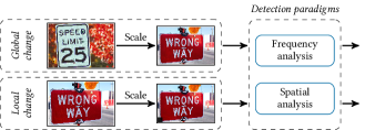
Figure 1. Image-scaling attacks: global modification (top) and local modification (bottom). Note the small box (backdoor) on the lower left that appears. Both attacks can be detected by using a frequency or spatial analysis.

Two defense strategies have been explored for addressing this threat: prevention and detection. In the first case, robust scaling algorithms or specific defense filters are applied to input images to prevent attacks. While these defenses are provably effective, as demonstrated by Quiring et al. (2020), they can only prevent but not detect attacks. However, detection can be necessary in various cases: First, we can spot on-going attacks. This allows scanning image collections for attacks or identifying the adversary. Second, robust algorithms like area scaling are slower compared to vulnerable algorithms, so that a one-time check might be preferred in real-time settings. Third, detection allows protecting proprietary learning systems where components cannot be changed.

The detection of image-scaling attacks, however, has not been rigorously studied yet. In this paper, we address this research gap and present the first in-depth systematization and analysis of detection methods for image-scaling attacks. We identify two general paradigms that underlie existing detection approaches: frequency analysis and spatial analysis. In the first paradigm, the detection is based on searching for conspicuous traces in the frequency spectrum. In the second paradigm, the pixels are analyzed, either by leveraging the adversarial modification or the remaining clean pixels for further analysis.

We derive novel detection methods for these paradigms that are simple yet effective in spotting image-scaling attacks. Our methods significantly outperform previous approaches, as we can reduce heuristic elements and precisely pinpoint the detectable characteristics of image-scaling attacks.

We demonstrate the efficacy of our methods in a comprehensive evaluation. In contrast to prior work, we study the detection performance with a diverse evaluation setup, including all major learning platforms, scaling algorithms, a large dataset, static & adaptive adversaries, and different attack scenarios such as global & local changes. If the entire scaled image is modified, both paradigms allow a detection rate between 99% and 100%. Our frequency approaches are particularly effective with a perfect detection rate. In the challenging scenario where only a local area is manipulated, previous methods fail while the newly derived approaches remain effective. The frequency paradigm enables a detection rate of 90%. The spatial paradigm allows detecting at least three out of four attacks. Under an adaptive attacker, however, the paradigms’ effectiveness flips: The frequency paradigm—the strongest in the static attack—does not withstand an adaptive attack while the spatial analysis remains robust. As a result, we conclude that both paradigms should be used in combination to complement each other.

Contributions

In summary, our contributions are as follows:

1. Systematization of detection. We present the first systematic analysis of detection methods for image-scaling attacks where we identify two general paradigms.

2. Novel approaches to detection. Based on our analysis, we derive novel detection approaches that significantly outperform all approaches from previous work.

3. Comprehensive evaluation. We empirically investigate the performance of all detection approaches in a comprehensive evaluation that covers all major learning platforms and scaling algorithms.

4. Different attack models. Moreover, we carefully examine the limits of all detection approaches by experimenting with different attack scenarios, such as global & local changes, and with both static & adaptive attackers.

To foster further research in this area, our code is publicly available at https://github.com/EQuiw/2023-detection-scalingattacks.

Roadmap

We introduce image-scaling attacks in Section 2. The detection paradigms with our new methods are presented in Section 3 and the evaluation of their performance is given in Section 4. Adaptive attacks are evaluated separately in Section 5. Finally, Section 6 discusses related work and Section 7 concludes the paper.

2. Background

We start by introducing the background on image-scaling attacks before presenting our novel detection approaches.

2.1. Preprocessing in Machine Learning

When solving tasks of computer vision, image data is typically normalized and preprocessed before features are extracted and learning models are applied. In particular, image scaling is a widely used preprocessing step to bring images to a normalized form. Most learning algorithms expect a fixed input size and thus images with different or larger dimensions need to be scaled. For example, the deep neural networks VGG19 (Simonyan and Zisserman, 2014) and ResNet (He et al., 2016) require inputs of $224\times 224$ pixels. Due to this frequent preprocessing, major machine-learning frameworks directly integrate different scaling algorithms. For instance, Caffe employs the image processing library OpenCV, PyTorch uses the library Pillow, and TensorFlow has its own implementation called tf.image. Following prior work (Xiao et al., 2019), we thus focus our analysis on the libraries OpenCV, Pillow, and tf.image with their respective implementations of scaling algorithms.

2.2. Image-Scaling Attacks

Interestingly, the downscaling of images leads to a considerable attack surface in learning-based systems. By carefully modifying particular pixels, it becomes possible to control the output of the scaling algorithms and thus to change the content of the scaled image. In the following, we recap the current state-of-the-art of these image-scaling attacks (Xiao et al., 2019; Quiring et al., 2020).

Figure 2 exemplifies the principle of the attack. Given a source image $S$, the adversary tries to find a minimal perturbation $\Delta$, so that the downscaling of the modified image $A=(S+\Delta)$ produces an output image, $\mathrm{scale}(A)$, that matches the adversary’s target image $T$. This attack can be modeled as a quadratic optimization problem:

$$\min(\|\Delta\|_{2}^{2})$$

(1) $$\mathrm{s.t.}\quad \|\mathrm{scale}(S+\Delta)-T\|_{\infty}\leqslant\epsilon\text{ and }A\in\mathit{R},$$

where the interval $\mathit{R}$ is the allowed pixel range, as for example, $\mathit{R}=[0,255]$ for 8-bit images.

Figure 2. Principle of image-scaling attacks: The adversary finds a minimal modification $\Delta$ of $S$ such that the modified image $A=(S+\Delta)$ still looks like $S$, but downscales to $T$.

To deceive the victim, a successful attack has to fulfill two objectives: First, the scaled image, $\mathrm{scale}(A)=\mathrm{scale}(S+\Delta)$, needs to match the target image $T$, i.e., $\mathrm{scale}(A)\sim T$. Second, the attack image should be indistinguishable from the source image, i.e., $A\sim S$. As a result, the adversary gets an attack image $A$ that looks identical to the source $S$ but changes to the target $T$ after downscaling.

This attack is independent of the training data, extracted features, and employed learning model. The adversary only needs to know the used scaling algorithm and the target size of the scaled image. In practice, this knowledge might not be difficult to obtain. Publicly available deep neural networks are often re-used through transfer learning. Moreover, the number of possible scaling configurations in the libraries is limited. In some settings, the knowledge about the algorithm is not even required. OpenCV and TensorFlow, for example, are effectively using nearest scaling when the scaling factor is an (uneven) integer (Quiring et al., 2020). This simplifies an attack if the adversary can choose the size of $S$. Finally, even without any knowledge, the scaling setup can be deduced through black-box queries (Xiao et al., 2019).

Threat Scenario

By attacking the preprocessing, the input is manipulated at the very beginning of the learning pipeline. An adversary can thus efficiently control any subsequent steps, which enables and simplifies different attack strategies. First, during training time, the attacker can conceal poisoning and backdoor attacks: The training-data modifications become visible only after downscaling (Quiring and Rieck, 2020). This alleviates the shortcoming of attacks that leave visible artifacts in images (Gu et al., 2017; Yao et al., 2019; Shafahi et al., 2018). The combination is useful, for example, if backdoors are used in the physical world. At training time, scaling attacks hide the trigger that can be later activated in the physical world. Second, during test time, the adversary can control the predictions of a learning model—without modifying the training data or model. The adversary uses the scaling attack, so that the downscaling leads to an image of the target class.

Note that scaling attacks allow a similar attack as adversarial examples by causing a misclassification. However, they do not depend on the learning model or features, since the scaling stage produces a perfect image of the target class. Scaling attacks would succeed even if neural networks were robust against adversarial examples.

Attacks can be realized with varying degrees of modification. We differentiate two scenarios to understand the detection capabilities:

• Global modification. The adversary chooses a target image with an arbitrary, unrelated content. The input $S$ and target $T$ have no relation to each other. This is the most severe attack, as any target class can be chosen.

• Local modification. The source and target image are identical, except for a limited area. We study backdoors as example for this category where only a small trigger is added (see Figure 9). A detection is challenging due to the small changes.

When studying the global scenario, we also consider an overlay scenario where the scaling attack only partially creates the target image $T$. Here, we blend $T$ into the downscaled source image to create a novel target image. This scenario allows us to study an attacker who does not fully embed the target image into the scaling output.

Root Cause

Image-scaling attacks are possible because scaling algorithms do not process all pixels equally (Quiring et al., 2020). Depending on the algorithm and scaling ratio, many pixels in $S$ have limited or even no impact on the scaled output. An adversary can therefore only modify those pixels that are considered during scaling. The resulting sparse noise is visually imperceptible, yet controls the entire output of the scaling process (see Figure 3). In this way, both attack objectives, $\mathrm{scale}(A)\sim T$ and $A\sim S$, are fulfilled. We build our detection defenses on this understanding of scaling attacks.

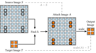
Figure 3. Simplified illustration of the root cause of image-scaling attacks: The scaling algorithm considers only a few pixels in an input $S$ (visualized by a thicker box). The adversary has to change only these pixels to control the downscaling output. This added noise is not noticeable.

Prevention Defenses

We also recap defenses that prevent image-scaling attacks. Prior work has studied two concepts: First, we can apply a robust scaling algorithm that considers all pixels with equal contribution. This directly addresses the root cause of the attack, since no pixels are ignored anymore. A possible scaling algorithm is area scaling that is implemented in several image processing libraries. Second, the defender can use an image-reconstruction method to repair the modified pixels from their neighborhood. To circumvent this defense, an adversary would have to modify the neighborhood as well, which leads to visible modifications. We refer the reader to the paper by Quiring et al. (2020) which examines both concepts and their robustness.

While prevention mechanisms do not interfere with the typical machine-learning workflow, they have a clear disadvantage: The mechanisms cannot be applied to find out that an attack is going on, that is, the data is manipulated. However, this can be necessary to ensure that we can trust a specific dataset, for instance, if we use publicly available images or release our image database. Hence, there is a need to study effective detection methods as complementary approach to existing prevention concepts.

3. Detection Systematization

The detection of image-scaling attacks has received little focus so far. While some heuristics have been proposed (Kim et al., 2021; Xiao et al., 2019), we still lack a general understanding on how the attacks can be effectively characterized and detected. To fill this gap, we systematize existing work by identifying two general detection paradigms. For each paradigm, we present the basic principle of detection and introduce own realizations that alleviate shortcomings of existing heuristics. Table 1 shows an overview of all considered detection methods.

Table 1. Overview of detection methods in this paper.

Paradigm		Method	Options
Frequency		*  Peak Spectrum
		*  Peak Distance
		*  CSP (Kim et al., 2021)
		*  CSP–improved
Spatial	Adversarial	*  Down & Upscaling	PSNR
		*  Down & Upscaling	$\{$Histogram, Color-scattering$\}$ (Xiao et al., 2019)
		*  Down & Upscaling	$\{$MSE, SSIM$\}$ (Kim et al., 2021)
		*  Maximum filter	$\{$MSE, SSIM$\}$ (Kim et al., 2021)
		*  Minimum filter	$\{$MSE, SSIM$\}$ (Kim et al., 2021)
	Clean	*  Clean Filter	$\{$Median, Random$\}$+$\{$PSNR, SSIM$\}$
		*  Patch-Clean Filter
		*  Targeted Patch-Clean Filter

• * =Proposed in this paper.

• $\{.\}$ denotes a set of possible options for a respective method.

3.1. Paradigm: Frequency Analysis

In this paradigm, the detection builds on analyzing the frequency spectrum of images. This is a common procedure in computer vision and multimedia security (Sencar and Memon, 2013). In this frequency representation, periodical patterns become evident that are not detectable in the spatial image domain (pixel domain) (Kirchner and Böhme, 2008). In general, a frequency spectrum is an equivalent representation of an image that describes the pixels by a sum of waves oscillating at different frequencies (Smith, 1997). In this work, we use the 2D discrete Fourier transform (DFT) and work on the centered log-scaled magnitude spectrum (as visible e.g. in 4(a)). Intuitively, each coefficient in this magnitude spectrum shows the impact of a particular frequency for the image. The log-scaling emphasizes smaller values. The middle of the magnitude spectrum corresponds to low frequencies while higher frequencies are located towards the corners.

As the root-cause analysis of image-scaling attacks in Section 2 highlights, the adversary injects pixels from the target image $T$ into $S$ in a periodic distance. This periodicity stems from the sampling process of image scaling and provides a strong indicator of image-scaling attacks. Hence, a modified image has unique, periodic peaks in its frequency spectrum. As an example, let us analyze the running example in Figure 2. The modification is not visible in the spatial domain. However, if we analyze the attack image in the frequency domain—as visible in 4(b)—one can clearly see unusual frequency peaks.

Proposed Detection

For our analysis, we take inspiration from multimedia forensics (Sencar and Memon, 2013; Chen and Hsu, 2011). We start by noting that the defender exactly knows the potentially modified pixels in the spatial domain. This allows an exact computation of the expected peak locations in the frequency spectrum. As a result, we gain the advantage of differentiating adversarial peaks created by scaling attacks from benign peaks that images can naturally have at other locations in the spectrum, reducing the chances to detect benign peaks accidentally.

In particular, our detection approach proceeds as follows: Let $(m,n)$ be the height and width of the source image and $(m^{\prime},n^{\prime})$ the height and width of the scaled output image. The vertical scaling ratio is given as $\beta_{m}=\tfrac{m}{m^{\prime}}$ while the horizontal scaling ratio is $\beta_{n}=\tfrac{n}{n^{\prime}}$. The constants $c_{m}$ and $c_{n}$ are the index of the spectrum’s middle. In the case of a scaling attack, the following binary function $\Gamma\in\{0,1\}^{m\times n}$ shows at which frequency coefficient a peak occurs:

(2) $$\Gamma(u,v)=\begin{cases}1&(u,v)=(c_{m}+k_{1}\cdot m^{\prime},c_{n}+k_{2}\cdot n^{\prime})\\ 0&\text{otherwise}.\end{cases}$$

$$\text{with}-\tfrac{\beta_{m}}{2}\leqslant k_{1}\leqslant\tfrac{\beta_{m}}{2},\;-\tfrac{\beta_{n}}{2}\leqslant k_{2}\leqslant\tfrac{\beta_{n}}{2},\;k_{1},k_{2}\in\mathbb{N}.$$

In other words, we expect to observe peaks around each $k_{1}m^{\prime}$-th and $k_{2}n^{\prime}$-th position of the frequency spectrum if an image is manipulated by an image-scaling attack. In Appendix A, we derive Equation 2. To provide some intuition, 4(c) marks the expected peaks on the frequency spectrum of our running example by using Equation 2. One can see that the observed and expected peaks match exactly. Equipped with the ability to predict the expected peaks, we propose two detection strategies.

Peak Spectrum.  We extract the frequencies in a square window centered around all expected peak locations. The window’s half length is $w$. We omit the center $(c_{m},c_{n})$ being present in any spectrum. 5(a) illustrates the resulting windows. Next, we average all window values and calculate the percentile rank of this value relative to the whole frequency spectrum. This sets the peak frequencies into relation to the entire frequency spectrum. In case of an attack, the peak frequencies outshine the entire spectrum, so that attack images get higher percentile ranks than benign images.

Peak Distance.  We divide the spectrum into excerpts for each peak as 5(b) visualizes. We discard the center of the spectrum again. For each excerpt, we extract the maximum peak and calculate the distance between this peak and the expected peak. We then average all measured distances. In case of an attack, this average is expected to be small.

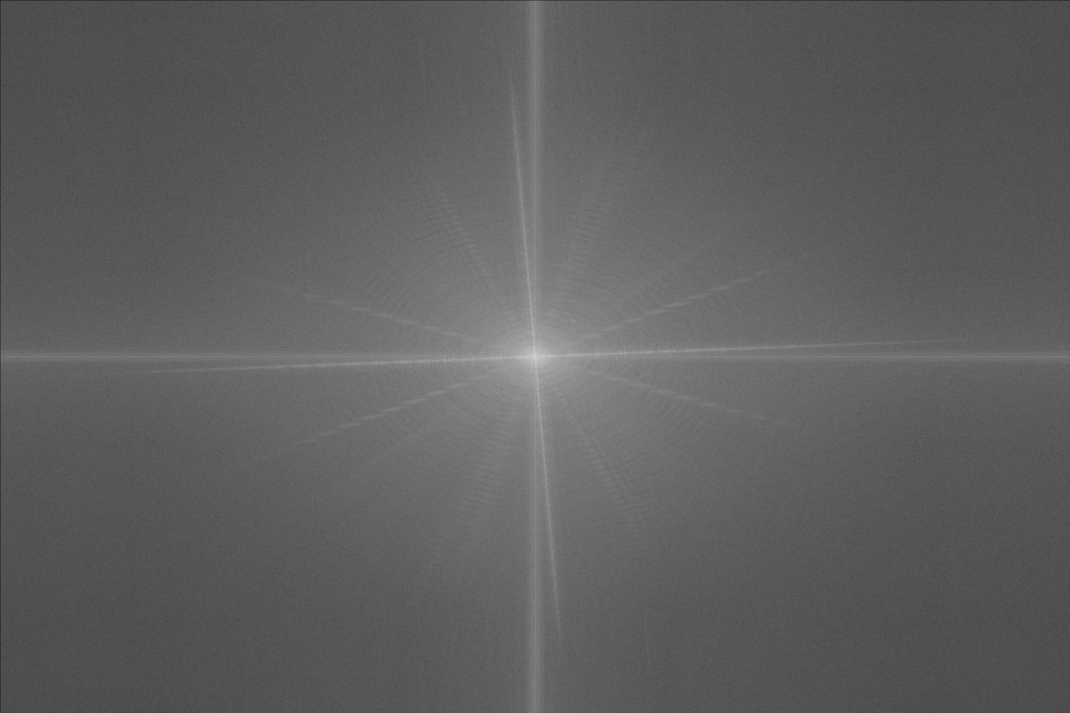
(a) Spectrum of $S$

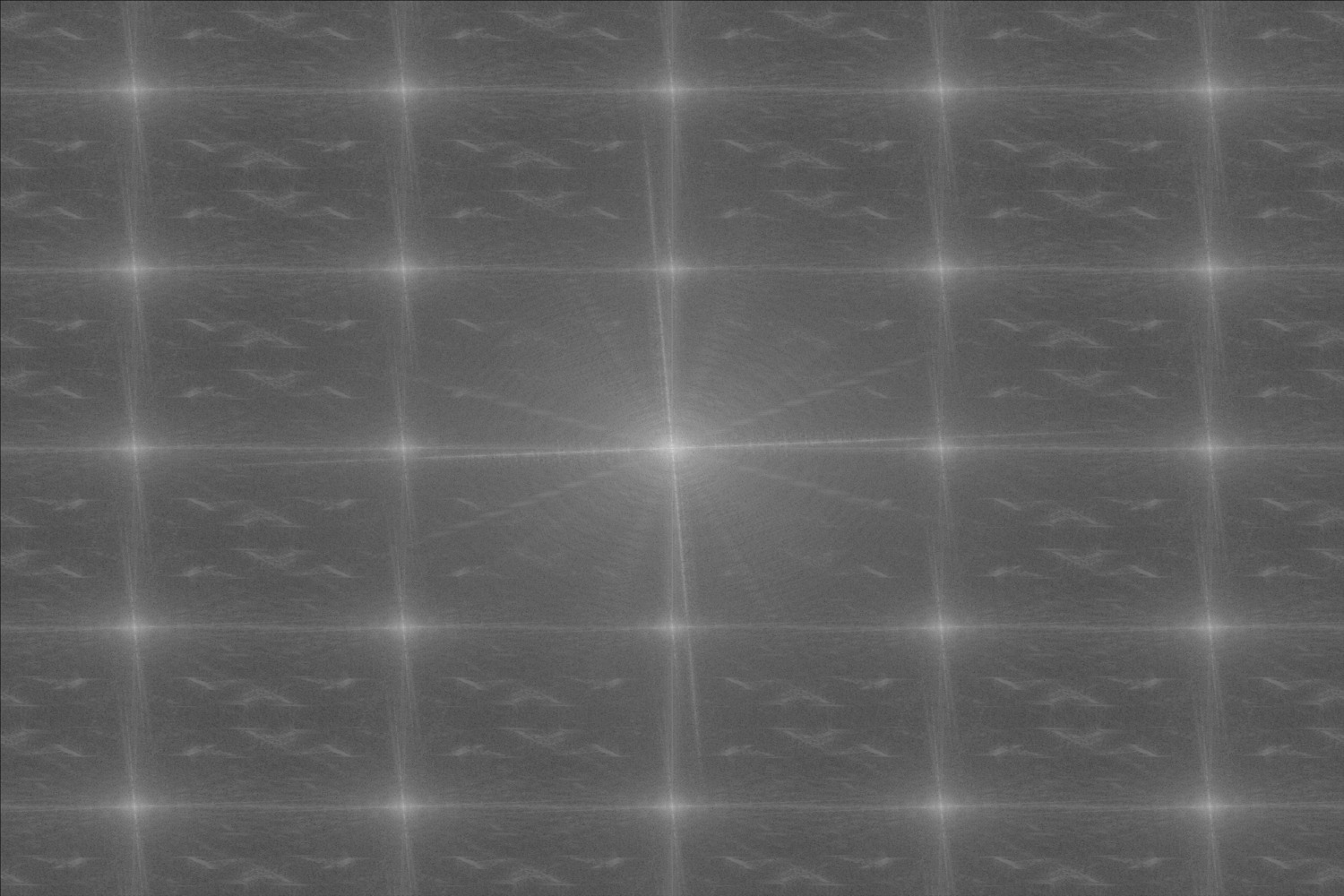
(b) Spectrum of $A$

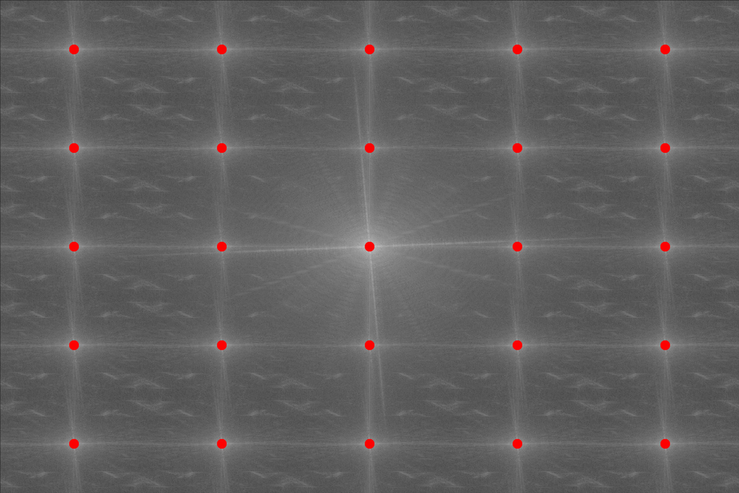
(c) Marked peaks in $A$

Figure 4. Frequency analysis of the example in Figure 2. Plot (a) and (b) show the frequency spectrum of the source image and attack image, respectively. Plot (c) shows the marked peaks with Equation 2.

Previous Approaches

Kim et al. (2021) propose a frequency analysis, named CSP, where the underlying idea is to count peaks at arbitrary positions in the spectrum. Based on their evaluation, they assume an attack if the spectrum contains more than one peak. Our evaluation shows that this approach is ineffective. Benign images can naturally have peaks, too. We show two such examples from ImageNet in Appendix B. To test if the method works without the fixed threshold of one, we evaluate an own adjustment, named CSP-improved, where we derive the threshold from the data. Still, this adjustment cannot compete with our methods. The defender should rather use the advantage of having precise knowledge about the expected peak locations—as our proposed methods do.

3.2. Paradigm: Spatial Analysis

In this paradigm, the analysis is done in the spatial domain. As scaling algorithms and scaling attacks operate here, this domain naturally provides the advantage of knowing which pixels are considered by scaling algorithms and hence which are possibly modified. We identify two variants of this paradigm: A defense leverages either the adversarial modification or the clean pixels in $A$ for detection. In the following, we examine each group in more detail.

3.2.1. Adversarial-Signal Driven

The concept here is to amplify the sparse, adversarial modifications in $A$ and then to compare the amplified image $A^{\prime}$ with $A$. We have two sub-groups here.

Down-and-Upscaling

We can exploit that downscaling and upscaling form antagonists in the spatial domain. That is, the scaling of $A$ leads to an output $D$ which corresponds to $T$. By upscaling $D$ back to the original size, $A^{\prime}=\mathrm{upscale}(\mathrm{downscale}(A))$, we can compare this version with $A$. The upscaling strengthens the signal embedded by the adversary and renders it detectable through comparison with the original image. Note that the comparison function needs to account for this setup, as we describe later.

In principle, we do not need to upscale the image and could directly compare $A$ with $D$. In our preliminary experiments, however, we found that we can achieve better results if we upscale $D$ to the resolution of $A$ and conduct the comparison on the same dimensions. Moreover, some image comparison methods require the same size for the inputs.

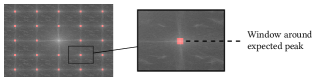
(a) Peak-Spectrum Analysis

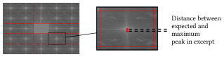
(b) Peak-Distance Analysis

Figure 5. Frequency-based detection approaches. Plot (a): Windows around expected peaks are extracted and their frequencies are compared in relation to the overall spectrum. Plot (b): Spectrum is divided into excerpts and the distance between expected and maximum peak for each excerpt is computed.

Proposed Detection.  A variety of methods exists for comparing images that would be applicable here. We find that a simple PSNR computation is particularly effective. Peak signal-to-noise ratio (PSNR) is a widely used pixel-based comparison method that returns the normalized mean-squared error between two images. Formally, it is defined as

(3) $$\mathrm{PSNR}(A,A^{\prime})=20\log_{10}(I)-10\log_{10}(\mathrm{MSE}(A,A^{\prime})).$$

The constant $I$ is the maximum of the pixel range, such as 255 for 8-bit images. The higher the PSNR value is, the more two images match. PSNR can be computed efficiently and thus provides a perfect basis for designing a detection method using down- and upscaling.

Previous Approaches.  Xiao et al. (2019) propose two alternative comparison options. First, the intensity histograms of $A$ and of $A^{\prime}$ are extracted and compared. Second, in the color-scattering method, the average distance to the image center over all pixels with the same intensity is computed. By doing this for each intensity value in $A$ and $A^{\prime}$, respectively, we obtain two vectors that can be compared. Moreover, Kim et al. (2021) propose two measures that directly compare $A$ and $A^{\prime}$: the mean squared error (MSE) and the SSIM index. While the first is simply comparing $A$ and $A^{\prime}$ pixel-wise, the latter aggregates information about the luminance, contrast, and structure between $A$ and $A^{\prime}$ (Horé and Ziou, 2010).

In our evaluation, the simple PSNR and SSIM outperform the other measures. Unlike suggested by prior work (Kim et al., 2021), MSE is not superior to PSNR. We assume that this conclusion is the result of a subtle implementation mistake in the evaluation metric where an integer overflow occurs. In fact, the PSNR and MSE are directly related to each other (see Equation 3). Although MSE and PSNR have the same detection performance, the PSNR score is easier to interpret. It typically lies between 0 dB and 60 dB in our evaluations. Moreover, in terms of security, a pixel-wise measure such as the PSNR is particularly robust against adaptive attacks compared to aggregation-based measures such as the histogram or color-scattering. No information are lost that could be exploited (Quiring and Rieck, 2020).

Amplifying Filter

As alternative to down-and-upscaling, Kim et al. (2021) propose two methods, a minimum filter and a maximum filter, to strengthen the adversarial signal. Each filter is applied on $A$ by iterating over the image and replacing each pixel by the minimum/maximum of its neighborhood. The outcome $A^{\prime}$ is compared with $A$ using MSE or SSIM. This filtering strategy aims at amplifying the periodic modification. However, as the CSP approach, this defense overlooks the attack’s root cause and misses the advantage of knowing the pixels used by scaling algorithms. A targeted filtering is possible which motivates our next group of defenses.

3.2.2. Clean-Signal Driven

Another concept of the spatial paradigm is to leverage the clean pixels that a scaling attack needs to leave to keep the attack imperceptible. We can use these pixels to clean $A$ and to compare this result with the initial version. This principle has not been studied before. It allows us to design specialized methods for the global and local attack scenario, which are presented in the following.

Proposed Global Detection

To obtain a cleansed version of $A$, we adopt the idea of reconstructing the modified pixels using prevention filters (Quiring et al., 2020). In particular, we design two methods that are based on a selective median filter and a selective random filter, respectively. Both filters repair each pixel considered by a scaling algorithm by using the neighborhood of the particular pixel. In terms of security, the reconstruction methods have the advantage of addressing the root cause of scaling attacks. They also show a strong robustness against adaptive attacks, since adversaries have to modify the neighborhood as well to bypass both filters, making the attack clearly visible (Quiring et al., 2020). This security robustness also transfers to our detection defense.

For detection, we propose the following simple clean filter approach: Equipped with a prevention filter $\mathcal{V}$, we can get a cleaned version $A^{\prime}=\mathcal{V}(A)$ which is compared with the initial input $A$. We evaluate the PSNR and the SSIM measure to compare $A$ and $A^{\prime}$.

Note that we also tested to compare $D$ and $D^{\prime}$ where $D^{\prime}$ is the downscaled version of $A^{\prime}$. Hence, $D$ shows the new adversarial content, while $D^{\prime}$ shows the original content. The detection results correspond to the clean-filter method and are thus omitted.

Proposed Local Detection

A direct application of the previous approach to the local attack scenario is not promising. As $A$ and $A^{\prime}$ are here similar for the majority of pixels, a global comparison cannot sufficiently capture the difference. Instead, we propose to divide the images into patches and compare each patch individually. We propose two variants.

Patch-Clean Filter.  We create $D$ and $D^{\prime}$ and divide them into $L$ patches, respectively. We compute the PSNR between each pair of patch, $v_{i}=\mathrm{PSNR}(D_{i},D^{\prime}_{i})\;\forall i=1,\dots,L$. The final detection score is given as $|\mathrm{mean}(\{v_{i}\})-\mathrm{min}(\{v_{i}\})|.$ Appendix C presents the method in more detail. Note that we work on downscaled images here. We find that the smaller image size reduces the number of possible regions which improves the detection rate.

Targeted Patch-Clean Filter.  As alternative, we analyze the unscaled images. However, even with patches, the scaling pixels—and thus modified pixels—are in the minority, making it difficult to detect a difference with and without scaling attack. Hence, we propose a more targeted variant and only examine the scaling pixels in each patch. Let $L$ denote the number of patches, $A_{i}$ & $A^{\prime}_{i}$ the respective patches, and $\Psi$ the scaling-pixel selection, we compute

(4) $$u_{i}=|\Psi(A^{\prime}_{i})-\Psi(A_{i})|\quad\forall i=1,\dots,L\;.$$

We get the $q$-th quantile of each vector $u_{i}$, denoted as $\mathrm{q}(u_{i})$, and calculate $|\mathrm{max}(\{\mathrm{q}(u_{i})\})-\mathrm{mean}(\{\mathrm{q}(u_{i})\})|$ as detection score. This comparison allows us to identify an unusual difference in a local area. Note that the choice of $q$ is a hyperparameter of the method.

Remark.  We also tested the down-and-upscaling concept with patches. However, $A^{\prime}=\mathrm{upscale}(\mathrm{downscale}(A))$ contains a stronger noise signal due to down-and-upscaling. While this is tolerable in the global scenario, it distorts the comparison with small patches.

4. Evaluation

We proceed with an empirical evaluation of the different detection methods. To obtain a comprehensive view, we study both non-adaptive and adaptive adversaries. In this section, we consider the non-adaptive case with regular attacks. Then, in Section 5, we investigate the best approaches against an adaptive adversary.

4.1. Evaluation Setup

Our evaluation follows the common design of experiments on image-scaling attacks (Xiao et al., 2019; Quiring et al., 2020). We evaluate the detection of attacks against popular scaling algorithms that are vulnerable to scaling attacks (Quiring et al., 2020). In particular, we consider nearest-neighbor, bilinear, and bicubic scaling from the libraries OpenCV and tf.image (TensorFlow), and nearest-neighbor scaling from the library Pillow. We omit Lanczos scaling which is comparable to bicubic scaling (Quiring et al., 2020).

For the attacks, we adopt the evaluation setup by Quiring et al. (2020), where the source and target for an attack are randomly drawn from a collection of images. As dataset for this sampling, we use photos from ImageNet (Russakovsky et al., 2015). Compared to other datasets from computer vision, like CIFAR or CelebA, ImageNet contains significantly larger images, which is a key requirement for constructing successful scaling attacks in practice. Moreover, the dataset is very diverse, covering various image sizes and contents, such as faces, animals, persons, objects, and landscapes.

As learning model, we use a pre-trained VGG19 model (Simonyan and Zisserman, 2014) which is a standard benchmark in computer vision. The target size for scaling is thus $224\times 224\times 3$ pixels. Note that we just use this one architecture in our experiments, since scaling attacks do not depend on the learning model’s architecture. They change the input to the model. Only the input size of the model is relevant, so that we make sure to use varying scaling ratios as described later. Finally, we consider a global and local modification scenario. Both require a slightly different setup that we present in the following.

Global Modification

To obtain attack images in this scenario, we randomly sample images from ImageNet and create 1,000 source–target image pairs. We ensure that the pairs have varying scaling ratios to avoid artifacts that may arise from a fixed ratio. We check that each target is unrelated to its source image by requiring different classes and predictions for each pair. After conducting the attacks, we keep only those images that are successful regarding both attack objectives, i.e., $\mathrm{scale}(A)\sim T$ and $A\sim S$. To this end, we use the same methodology as Quiring et al. (2020). The number of successful images varies across each combination of scaling algorithm and library, so that we choose the highest possible number of images across all setups. This leads to 585 attack images for each combination of scaling algorithm and library. As unmodified reference set, we additionally select 585 further images from ImageNet. They are used to evaluate the detection of benign inputs.

Local Modification

Here, we implement the BadNets backdoor attack (Gu et al., 2017) as a representative form for local triggers that are also used in recent works (e.g., Salem et al., 2022). We use the same 585 source images as in the previous scenario. Yet, we scale each source image to a size of $224\times 224\times 3$ pixels and add a small, bounded backdoor pattern to create its respective target image (see Figure 9 in the Appendix). Finally, we conduct scaling attacks on these image pairs. As reference set, we use the same 585 benign images as before. We also verify that the so-created backdoors are effective (see Appendix D).

Evaluation Measures

To evaluate the detection performance of the considered detection methods, we equally split each attack and reference dataset into a training and test partition, respectively. The training set is used to calibrate a threshold for each detection method so that the false positive rate is 1%. This threshold is then used to evaluate the detection performance on the test set. For some detection methods, we need to decide on specific hyperparameters, such as the window width in the peak-spectrum analysis. For this calibration, we split the training set further and create a validation set. This set is used to find the optimal parameters in a grid search. We instantiate the detection methods with the best parameters (see Appendix E) and report their performance on the test set.

4.2. Global Modification Scenario

We start with the detection when source and target image are arbitrary. This is the most severe setting as an adversary can freely choose the target class of the prediction.

Results

Table 2 shows the performance for all detection methods, sorted in descending order with respect to the average accuracy. Both paradigms allow detecting scaling attacks if the entire scaled image is modified. A perfect detection is possible with our proposed peak-distance frequency analysis. However, not all methods are effective, such as the previously proposed CSP approach with an accuracy of 50%.

*  Method	Option	AvgAcc	StdAcc	AvgFPR
*  Peak Distance		100.00	00.00	00.00
*  Peak Spectrum		99.90	00.26	00.00
*  Clean Filter	Median filter, SSIM	99.80	00.21	00.05
*  Down & Up	Histogram	98.85	01.09	00.49
*  Down & Up	PSNR	98.54	01.48	00.49
*  Down & Up	MSE	98.54	01.48	00.49
*  Clean Filter	Random filter, SSIM	98.54	01.51	00.63
*  Targeted Patch-Clean Filter		96.54	04.16	00.88
*  Clean Filter	Median filter, PSNR	94.30	06.06	01.07
*  Maximum Filter	SSIM	87.03	03.53	01.80
*  Minimum Filter	SSIM	85.15	04.11	01.66
*  Clean Filter	Random filter, PSNR	81.52	08.59	01.17
*  CSP	Improved	76.72	06.19	01.32
*  Down & Up	SSIM	76.21	12.95	01.46
*  Minimum Filter	MSE	64.65	03.15	01.61
*  Maximum Filter	MSE	60.63	01.39	01.66
*  Down & Up	Color-scattering	55.88	03.70	00.83
*  CSP	Original	50.00	00.00	00.00
*  Patch-Clean Filter		49.95	00.08	00.10

Table 2. Detection performance [%] in global scenario in terms of accuracy (average + standard dev.) and false positives (average) over all scaling algorithms and libraries.   * Proposed in this paper.

Analysis

A closer look on this experiment provides important insights. First, our proposed frequency methods—exploiting the known peak locations—outperform all other detection methods. Their accuracy is 100% and 99.90%. On the other hand, the CSP approach (Kim et al., 2021) that also analyzes the frequency spectrum is comparable to random guessing. Second, the choice of the comparison function in the spatial paradigm is important. SSIM is preferable for the clean, minimum, and maximum filter. PSNR provides a higher detection accuracy with the down-and-upscaling approach. There is no difference between MSE and PSNR in our experiments. Third, patch-based defenses designed for the local scenario are partly applicable in the global case. The targeted patch-clean filter has a detection rate of 96.54%.

Ensemble of Detection Methods

Next, we combine multiple methods as ensemble to increase the diversity of detection patterns. We test three ensembles: We use the best method from each paradigm, and we use the $K=\{3,4\}$ best methods (irrespective of the paradigm). Note that we choose the methods based on the results on the training dataset and not Table 2.

The first ensemble consists of peak distance and the clean filter (with Median, SSIM). The ensemble with $K=3$ consists of the first three entries in Table 2. The ensemble with $K=4$ uses Down & Up with PSNR as 4th method in addition. We use two voting strategies: We report an attack if the majority of methods or if at least one method flags an input, that is, one winner takes all.

Table 3 shows the performance. The K-best ensemble with $K=4$ and majority voting achieves an accuracy of 100% and a false-positive rate of 0%. In terms of security, an ensemble thus allows a perfect detection rate while increasing the difficulty for an adaptive attack, as different paradigms and methods have to be circumvented.

	Majority			One Winner Takes All
Ensemble	Acc	TPR	FPR	Acc	TPR	FPR
Best Per Paradigm	99.98 $\pm$ 0.06	100.00 $\pm$ 0.00	0.05 $\pm$ 0.13	—	—	—
$K$ Best ($K$=3)	99.98 $\pm$ 0.06	99.95 $\pm$ 0.13	0.00 $\pm$ 0.00	99.98 $\pm$ 0.06	100.00 $\pm$ 0.00	0.05 $\pm$ 0.13
$K$ Best ($K$=4)	100.00 $\pm$ 0.00	100.00 $\pm$ 0.00	0.00 $\pm$ 0.00	99.73 $\pm$ 0.17	100.00 $\pm$ 0.00	0.54 $\pm$ 0.33

Table 3. Ensemble in global scenario. Each cell shows the average $\pm$ standard deviation over all scaling libraries and algorithms. With two paradigms, both voting methods for “best per paradigm” have identical results, so that we omit the 2nd voting method in this case.

Overlay Scenario

In addition, we study the variation where a scaling attack is used to embed only a low-opacity version of $T$ into the downscaled output. More specifically, the novel target image is given as $T^{\prime}=\alpha\cdot T+(1-\alpha)\cdot\mathrm{scale}(S).$ The parameter $\alpha$ denotes the blending factor. In our experiments, we set $\alpha=0.3$ to test a challenging case with only a very small embedding of $T$.

Table 4 shows the performance. Our frequency approaches still provide a detection rate close to 100%. Even with a very low blending factor, periodic peaks are inevitably created in the frequency spectrum. On the contrary, the spatial paradigm is more affected by the overlay scenario. A pixel-based comparison is more difficult, as $T$ is embedded more weakly.

Comparing Scaling Algorithms and Libraries

We have presented aggregated results over all scaling algorithms and libraries so far. In Appendix F, we analyze the individual detection per scaling algorithm and library. We find no significant difference between the libraries. Moreover, the frequency methods and the leading methods in the spatial paradigm do not depend on the scaling algorithm.

Summary

The effective detection of image-scaling attacks is possible with both paradigms. The frequency paradigm allows for a perfect detection rate without any false positives in our experiments. Even in the overlay scenario, it enables spotting all attacks with high accuracy. We conclude that scaling attacks can be efficiently detected if an adversary performs a global modification.

4.3. Local Modification Scenario

In our next experiment, we test the detection performance in the challenging scenario where an adversary applies an image-scaling attack only to a small area of an image.

Results

Table 5 shows the results for all detection methods. Only our proposed frequency methods can effectively detect local scaling attacks with an average accuracy of 80.98% and 89.81%. Our patch-based approaches achieve an acceptable detection rate of 76.38% and 75.72%. The other methods are close to random guessing.

*  Method	Option	AvgAcc	StdAcc
*  Peak Distance		99.73	00.24
*  Peak Spectrum		99.71	00.13
*  Clean Filter	Median filter, SSIM	93.47	05.12
*  Down & Up	Histogram	92.54	06.91
*  Clean Filter	Random filter, SSIM	78.30	08.99

Table 4. Detection accuracy in overlay scenario. Only the effective approaches with AvgAcc ¿ 60% are shown.

*  Method	Option	AvgAcc	StdAcc	AvgFPR
*  Peak Spectrum		89.81	04.75	01.07
*  Peak Distance		80.98	02.83	01.17
*  Targeted Patch-Clean Filter		76.38	12.35	00.93
*  Patch-Clean Filter		75.72	04.91	01.71
*  Down & Up	Color-scattering	51.56	02.08	00.83
*  Down & Up	Histogram	50.44	01.13	00.73
*  Clean Filter	Median filter, SSIM	50.15	00.18	00.59
*  Clean Filter	Random filter, SSIM	50.02	00.06	00.49
*  CSP	Original	50.00	00.00	00.00
*  Maximum Filter	SSIM	49.85	00.06	01.02
*  Minimum Filter	SSIM	49.80	00.51	01.46
*  Clean Filter	Median filter, PSNR	49.78	00.16	00.98
*  Down & Up	MSE	49.68	00.35	00.83
*  Down & Up	PSNR	49.68	00.35	00.83
*  Clean Filter	Random filter, PSNR	49.68	00.12	01.02
*  CSP	Improved	49.63	00.32	00.73
*  Minimum Filter	MSE	49.61	00.26	01.41
*  Maximum Filter	MSE	49.59	00.19	01.17
*  Down & Up	SSIM	49.51	00.32	01.12

Table 5. Detection performance [%] in local scenario in terms of accuracy (average + standard dev.) and false positives (average) over all scaling algorithms and libraries.   * Proposed in this paper.

Analysis

Most methods of the spatial paradigm are not effective anymore. The reason is that scaling attacks change only a small area. Thus, most of the compared areas still correspond to the original image, making a comparison difficult. On the contrary, the frequency approach is still effective, because even a limited, modified image area causes periodic frequency peaks. However, the impact on the frequency spectrum is weaker, so that the performance decreases compared to attacks modifying the full image.

Ensemble of Detection Methods

We also study ensembles of detection methods with local modifications. For the best-per-paradigm ensemble, we consider peak spectrum and the targeted patch-clean filter. The $K$-best ensembles consist of the first $K$ entries in Table 5. We consider $K=\{3,4\}$, as we have only four effective approaches (see Table 5).

Table 6 shows the performance. With majority voting and $K$-best ensembles, the false-positive rate can be reduced to 0% by sacrificing some accuracy. In turn, the combination of majority voting and best-per-paradigm slightly improves the accuracy, but with more false positives. Note, however, that the peak-spectrum method alone would achieve an average accuracy of 91.76% at a comparable false-positive rate of 1.85%. Taken together, no ensemble outperforms the individual methods in any aspect. In terms of performance, the ensemble seems not directly beneficial. Yet, it provides benefits against adaptive attacks as we will see in Section 5.

Comparing Scaling Algorithms and Libraries

In Appendix F, we analyze the individual detection performance. The library has no effect, but we observe a duality with more advanced scaling algorithms: Frequency methods become better while clean-signal methods become worse. With local modifications, a defender should therefore choose the detection method based on the scaling algorithm.

	Majority			One Winner Takes All
Ensemble	Acc	TPR	FPR	Acc	TPR	FPR
Best Per Paradigm	92.00 $\pm$ 1.57	86.01 $\pm$ 4.00	2.00 $\pm$ 1.19	—	—	—
$K$ Best ($K$=3)	84.84 $\pm$ 1.96	69.67 $\pm$ 3.92	0.00 $\pm$ 0.00	91.66 $\pm$ 1.72	86.49 $\pm$ 3.52	3.17 $\pm$ 0.43
$K$ Best ($K$=4)	86.35 $\pm$ 1.45	72.70 $\pm$ 2.90	0.00 $\pm$ 0.00	91.10 $\pm$ 1.96	87.08 $\pm$ 2.81	4.88 $\pm$ 1.38

Table 6. Ensemble in local scenario. Each cell shows the average and standard deviation over all scaling libraries and algorithms.

Varying Backdoors

Next, we study the detection performance with more backdoors that differ in type and location. In addition to our previously used backdoor (a black box in the lower left corner), we examine (i) a black circle embedded in the upper right corner, and (ii) a rainbow-like box (Liu et al., 2018) embedded in the lower left corner. These backdoors allow us to study the impact of shape, filling, and location. The box and rainbow patterns, for instance, are common patterns in backdoor attacks (Liu et al., 2018; Salem et al., 2022; Quiring and Rieck, 2020). The first two columns in Figure 9 in the Appendix show examples for all backdoor types.

Table 7 shows the performance. While the box and circle are well detectable, the rainbow-backdoor is only detected in 3 of 4 cases. We attribute this to the mixed filling, which causes weaker peaks in the frequency spectrum. Moreover, for three methods, the circle backdoor is slightly better detectable than the box. This is because the circle is larger, consuming 305 pixels compared to 225 pixels by the box. We verified this by reducing the circle size. The detection rates then become similar to the box backdoor. In summary, we study multiple backdoor types with scaling attacks. Our approaches detect them, yet the performance relies on the backdoor type.

Varying Backdoors At Train–Test Time

So far, the training dataset for calibrating the detection methods have had the same backdoor as the test dataset. In practice, this might not be realistic. As a remedy, we study an additional scenario where the training dataset is calibrated on a different backdoor than the one used in the test dataset. We study the same three backdoor types as before.

Table 8 shows the detection rate of the peak-spectrum method as a matrix for all possible backdoor combinations during train and test time. Using different backdoors has no impact on the detection. The values in each column in Table 8 are almost identical, irrespective of the backdoor at training time. The other detection methods have the same behavior and are reported in Table 14 in Appendix G. We further describe the reasons for these results in Appendix G.

Method	Box	Circle	Rainbow
Peak Spectrum	89.81 $\pm$ 04.75	93.03 $\pm$ 02.82	78.77 $\pm$ 05.85
Peak Distance	80.98 $\pm$ 02.83	87.79 $\pm$ 02.22	68.36 $\pm$ 02.81
Targeted Patch-Clean Filter	76.38 $\pm$ 12.35	70.55 $\pm$ 14.26	67.89 $\pm$ 22.53
Patch-Clean Filter	75.72 $\pm$ 04.91	79.50 $\pm$ 05.93	68.50 $\pm$ 06.42

Table 7. Detection performance with varying backdoors (accuracy $\pm$ standard deviation). Only the four effective detection methods are shown.

	Backdoor Test-Time
Backdoor Train-Time	Box	Circle	Rainbow
Box	89.81 $\pm$ 04.75	93.03 $\pm$ 02.80	78.77 $\pm$ 05.85
Circle	89.66 $\pm$ 04.94	93.03 $\pm$ 02.82	78.35 $\pm$ 05.67
Rainbow	89.76 $\pm$ 04.81	93.00 $\pm$ 02.78	78.77 $\pm$ 05.85

Table 8. Performance of peak spectrum with varying backdoors at train–test time (accuracy $\pm$ standard dev.). The rows show the used backdoor at training time, the columns the backdoor at test time.

Overall, we conclude that we can also detect scaling attacks if the backdoor—used to calibrate the detection—is different to the finally used backdoor from the adversary. Only the backdoor type itself, such as a circle or rainbow-like backdoor, affects the detection.

Summary

Even in the challenging scenario where only a local image area is manipulated, a reliable detection is possible. However, only four approaches are effective: our frequency approaches based on peak spectrum and peak distance, as well as both patch-clean filters. Finally, our results show that the defender does not need to have an exact knowledge of the employed backdoor.

5. Adaptive Attacks

Finally, we study an adaptive attacker who is aware of the deployed detection method and adjusts the attack strategy accordingly. We examine the global and the local modification scenario again, but limit our analysis to only the successful methods from Section 4. Note that we now have to analyze the detection rate and both goals of a scaling attack. Let $\tilde{A}$ be the adaptive version of $A$, an attack has to fulfill: (O1) $\mathrm{scale}(\tilde{A})\sim T$, and (O2) $\tilde{A}\sim S$. The second goal O2 is evaluated with the PSNR. The first goal O1 is tested by computing the attack success rate (ASR). In the global scenario, we define the ASR as the ratio of matches in the top-5 predictions from VGG19 between $\tilde{A}$ and $A$. In the local scenario with backdoors, we define the ASR as the ratio of successful matches of the backdoor’s target class in the top-5 predictions. Appendix D provides more information on the finetuning setup to measure the ASR with backdoors.

5.1. Attacking the Frequency Paradigm

To mislead a peak analysis, an adaptive attacker has to hide the periodic traces caused by a scaling attack. In the following, we analyze different methods to achieve this.

Suppressing Frequency

We begin with a targeted attack against our peak-spectrum analysis. We shortly introduce the concept before presenting the empirical results.

Approach.  The idea is to suppress the frequency spectrum in the window that is used by the defense. In particular, let $F$ denote the frequency spectrum of the attack image and $\omega\in W$ each window used by the spectrum analysis. The spectrum is then manipulated as follows:

(5) $$F(A)[\omega]=f_{s}\cdot F(A)[\omega]\quad\forall\;\omega\in W,$$

where $f_{s}$ is a parameter to control the reduction and $[\cdot]$ selects a subset of frequencies. Figure 6 illustrates the adaptive attack by setting all frequencies in the window $\omega$ to zero.

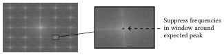
Figure 6. Adaptive attack by suppressing frequencies with $f_{s}=0.0$. Note that such a strong reduction is often not needed.

Results.  This adaptive attack has a strong impact on the detection performance, as Section 5.1 shows. The average detection accuracy notably decreases with a smaller value of $f_{s}$. Note that using $f_{s}=0.0$ leads to a too strong frequency reduction, so that the detection threshold could be simply inverted, increasing the accuracy, for instance, to 66.63% (100% - 33.37%) in the global case. To provide more intuition on the resulting image quality, Figure 10 in the Appendix shows an exemplary image from our evaluation for varying values of $f_{s}$.

Regarding the goals O1 and O2, the adaptive attack has only an impact in the global scenario. Here, the ASR decreases and the attack images loose brightness and contrast. The output images become a mixture between the original and novel content. On the contrary, in the local scenario, $f_{s}$ has no significant impact on the ASR and the visual quality. In summary, an adaptive attacker can notably decrease the detection performance. In the global scenario, however, the attacker has to sacrifice the goals O1 and O2 to some extent, which limits the impact of the attack.

		Detection		Attack O1	Attack O2
Attack	Option	AvgAcc	StdAcc	ASR	AvgPSNR	StdPSNR
Global Local

Table 9. Adaptive attack against peak-spectrum approach by suppressing frequency peaks (Acc. and ASR in [%], and PSNR in [dB]).

Add Frequency Peak

We continue with an attack against the peak-distance analysis. Again, we shortly introduce the concept before presenting results.

Approach.  The idea is to insert an additional peak in each excerpt so that the distance between the expected and maximum peak increases. Let $p\in P$ be the frequency location for adding a peak in each excerpt, the spectrum is modified as follows:

(6) $$F(A)[p]=f_{a}^{-1}\cdot\max{(F(A))}\quad\forall\;p\in P,$$

where $f_{a}$ controls the strength of the added peak. For simplicity, the peak locations $p\in P$ are the corners of each excerpt. Figure 7 illustrates the adaptive attack. This frequency modification is hard to perceive in the whole frequency spectrum, as only very nuanced changes are performed.

Results.  Section 5.1 shows the results of the adaptive attack. The peak addition has a strong impact on the detection performance. Already $f_{a}=75$ notably decreases the performance in the global and the local modification scenario. At the same time, the peak addition has only a minor effect on the goal O1. To better explain the effect on O2, Figure 11 in the Appendix shows an example from our evaluation. As $f_{a}$ decreases and the peaks become stronger, the images loose brightness and contrast. Still, the image content remains intact—even at a high modification factor with $f_{a}=25$. We thus conclude that O2 is also partly achieved. All in all, we identify a suitable range of $50\leqslant f_{a}\leqslant 75$ where the peak-distance approach does not detect an attack and both goals of a scaling-attack are satisfied.

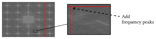
Figure 7. Adaptive attack by adding peaks with $f_{a}=25$. Note that our evaluation shows that such a strong addition is often not necessary.

		Detection		Attack O1	Attack O2
Attack	Option	AvgAcc	StdAcc	ASR	AvgPSNR	StdPSNR
Global Local

Table 10. Adaptive attack against the peak-distance approach by adding frequency peaks (Acc. and ASR in [%], and PSNR in [dB]).

JPEG Compression

As a baseline, we consider a generic and simple counterattack by examining JPEG compression. It is known to have an impact on resampling detectors in multimedia forensics (Kirchner and Böhme, 2008), which analyze the frequency spectrum for peaks similar to our approach. Appendix H presents the results. Compression only affects the local scenario. However, the effect on the detection performance is smaller compared to our previous two targeted adaptive attacks.

5.2. Attacking the Spatial Paradigm

Lastly, we discuss the attack surface of the other paradigm. For strengthening approaches based on down- and upscaling, an adaptive attack should not be possible. Upscaling algorithms do not suffer from the root cause that enables scaling attacks in the downscaling case. Upscaling algorithms usually use each pixel multiple times to compute the larger image, so that an attacker cannot hide a new signal. We verified the implementation of the imaging libraries OpenCV, Pillow, and tf.image (TensorFlow) and observed this behavior in their upscaling algorithms. Thus, if the downscaling reveals another content, the upscaled version will necessarily keep this content, making an adaptive attack difficult.

The clean-signal driven approaches based on prevention filters inherit the security properties of the respective filter. Prior work has demonstrated that these filters withstand adaptive attackers (Quiring et al., 2020). In the global scenario, we can thus conclude that the detection is robust. In the local scenario, however, the cleaning approach only works with a patch extraction. In this case, this patch extraction can introduce a new vulnerability. For example, an attacker could distribute a backdoor over multiple patches. This requires designing new backdoor methods which is beyond the scope of this paper.

5.3. Summary

Our analysis shows that the frequency paradigm, although the strongest under a static attacker, can be circumvented by an adaptive attacker. On the contrary, the spatial paradigm withstands adaptive attacks by design. Hence, we are faced with a trade-off where the frequency and spatial paradigms complement each other in detection capabilities and robustness, respectively.

6. Related Work

Image-scaling attacks are a novel threat to the security of machine-learning systems. As a result, there exists only a small body of related work that is discussed in the following.

Attacks.  Xiao et al. (2019) have initially introduced image-scaling attacks. Quiring et al. (2020) perform an in-depth analysis of scaling attacks and identify their root cause. We build our defenses on this understanding. Chen et al. (2020) extend the original attack by studying different norms for Equation 1. Yet, these norms do not affect the attack’s working principle and thus our proposed defenses. Quiring and Rieck (2020) examine the application for the poisoning and backdoor scenario. This work motivates our inclusion of the local-modification scenario. Finally, Gao et al. (2022) combine adversarial examples and scaling attacks. We excluded the attack, since it operates in a different threat scenario. The attack is dependent on the learning model and requires an iterative adversarial-example process. On the contrary, we focus on general scaling attacks that are model-agnostic and just create the target as scaling output.

Defenses.  To fend off scaling attacks, we can either prevent or detect an attack. In the former case, Quiring et al. (2020) have extensively studied prevention defenses. In the latter case, Xiao et al. (2019) and Kim et al. (2021) have presented first ideas, evaluated with non-adaptive attackers. We include these approaches in our comparison, but our evaluation shows that they are often ineffective.

Adversarial Learning.  Scaling attacks are preprocessing attacks (Quiring et al., 2020) that represent a new type of ML attack in addition to existing attacks, such as adversarial examples and poisoning (Biggio and Roli, 2018; Papernot et al., 2018; Quiring et al., 2019).

7. Conclusion

This paper is the first comprehensive study on the detection of image-scaling attacks. We examine the problem from multiple viewpoints by considering various scaling algorithms, levels of modification, and attacker models. We systematize the detection and derive novel approaches based on our improved understanding.

The frequency paradigm is the strongest detection approach in any image-modification scenario under a static attack. Under an adaptive attack, it is not robust and vulnerable to evasion. The spatial paradigm is suitable for spotting global manipulations but lacks accuracy for local changes. However, it enables a robust detection under adaptive attacks. Therefore, our results motivate that both paradigms should be used as ensemble to complement each other.

Finally, we emphasize that detection should not be seen as replacement for prevention defenses. In fact, both concepts best operate in combination. While prevention methods block attacks during training and inference, approaches for detection help identify on-going attacks and ultimately help tracking down adversaries. As a result, by combining both concepts, we can improve the security of machine-learning systems.

Appendix A Frequency Analysis

In the following, we derive the computation of the peak positions that an image-scaling attack inevitably introduces. We start with an uncentered view of the frequency spectrum as well as two assumptions that will be gradually relaxed: the use of nearest scaling and an integer as scaling ratio. This enables us to define a simplified image model. It mimics the blocking artifacts that a scaling attack will add in a periodic interval (recall the root-cause analysis in Section 2.2). In particular, we denote by $B\in\{0,1\}^{m\times n}$ an image where all values are set to 1, except for those on a grid in the interval $\beta_{m}\in\mathbb{N}$ along the vertical direction and in the interval $\beta_{n}\in\mathbb{N}$ along the horizontal direction:

(7) $$B(i,j)=\begin{cases}0&\text{if }i=l_{1}\beta_{m}\land j=l_{2}\beta_{n}\\ 1&\text{otherwise},\end{cases}$$

$$\text{with}\;\;0\leqslant l_{1}<m^{\prime},\;0\leqslant l_{2}<n^{\prime},\;l_{1},\;l_{2}\in\mathbb{N}.$$

The function $B$ corresponds to the image model for JPEG compression by Chen and Hsu (2011), except for a different periodicity between the peaks in the grid. Substituting the JPEG periodicity of 8 by the periodicity $\beta_{m}$ and $\beta_{n}$, we expect to observe peaks around each $k_{1}m^{\prime}$-th and $k_{2}n^{\prime}$-th position of the frequency spectrum if an image is manipulated by an image-scaling attack. More formally, we can define the following binary function $\Gamma\in\{0,1\}^{m\times n}$ that shows at which frequency coefficient a peak occurs:

(8) $$\Gamma(u,v)=\begin{cases}1&(u,v)=(k_{1}m^{\prime},k_{2}n^{\prime})\\ 0&\text{otherwise}.\end{cases}$$

$$\text{with}\;0\leqslant k_{1}<\beta_{m},\;0\leqslant k_{2}<\beta_{n},\;k_{1},k_{2}\in\mathbb{N}.$$

To bring this into a centered view, we shift the coordinates and get:

(9) $$\Gamma(u,v)=\begin{cases}1&(u,v)=(c_{m}+k_{1}\cdot m^{\prime},c_{n}+k_{2}\cdot n^{\prime})\\ 0&\text{otherwise}.\end{cases}$$

$$\text{with}\;-\tfrac{\beta_{m}}{2}\leqslant k_{1}<\tfrac{\beta_{m}}{2},\;-\tfrac{\beta_{n}}{2}\leqslant k_{2}<\tfrac{\beta_{n}}{2},\;k_{1},k_{2}\in\mathbb{N}.$$

The constants $c_{m}$ and $c_{n}$ are the index of the spectrum’s middle.

Let us now relax the assumptions. First, although scaling attacks manipulate more pixels for other algorithms such as bilinear and bicubic scaling, their manipulation still operates on a grid. Hence, Equation 9 can also be applied in these cases. Next, we relax the integer assumption of the scaling ratio. In practice, the ratio can also be a rational number. A closer analysis shows that the step width $\beta_{m}$ and $\beta_{n}$ can alternate in this case. As a result, we observe an additional periodic signal. The frequency spectrum has additional sub-peaks. Still, Equation 9 is also applicable in this case, as the major step widths correspond to $\beta_{m}$ and $\beta_{n}$. Yet, we set $k_{1}\in\mathbb{N}$ and $k_{2}\in\mathbb{N}$ in Equation 9 as follows: $-\tfrac{\beta_{m}}{2}\leqslant k_{1}\leqslant\tfrac{\beta_{m}}{2},\;-\tfrac{\beta_{n}}{2}\leqslant k_{2}\leqslant\tfrac{\beta_{n}}{2}$.

Appendix B Frequency Peaks in Natural Images

In Figure 8, we show two unmodified, benign image examples from ImageNet where the frequency domain naturally contains frequency peaks. The CSP approach would flag both images as attack. In the first image, for example, the periodic pattern of the radiator grill causes the peaks.

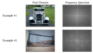
Figure 8. Unmodified examples from ImageNet with natural peaks.

Appendix C Patch-Clean Filter

Here, we provide more details on the patch-clean filter. Recall that we create two versions of $A$. First, we downscale $A$ directly using the vulnerable scaling algorithm, yielding $D$. Second, we apply a prevention filter $\mathcal{V}$ on $A$ and downscale $A^{\prime}=\mathcal{V}(A)$, yielding $D^{\prime}$. Hence, the adversarial modifications are present in $D$, while $D^{\prime}$ is a clean version. We only use the median filter for $\mathcal{V}$ in our evaluation. The filter better preserves the visual quality, which is important when small patches are used for comparison.

We apply a Gaussian filter on $D$ to smooth it slightly, as $D^{\prime}$ is slightly smoothed due to the previous application of $\mathcal{V}$. For simplicity, we fix the Gaussian kernel size to (3,3) and the kernel standard deviation to 0. Finally, we divide both images into patches. Let $D_{i}$ and $D^{\prime}_{i}$ denote corresponding patches from the same region in $D$ and $D^{\prime}$. Let $L$ be the number of patches. We compute $v_{i}=\mathrm{PSNR}(D_{i},D^{\prime}_{i})\;\forall i=1,\dots,L$. The final detection score is given as:

(10) $$|\mathrm{mean}(\{v_{i}\})-\mathrm{min}(\{v_{i}\})|.$$

If a scaling attack changes only a local area, only a few patches will have an unusually small PSNR value. Compared to benign images, the minimum over all patches is then significantly smaller than the mean. The difference between mean and minimum thus reveals local attacks. To obtain patches, we iterate over the image with a sliding window and extract sub-windows as patches. The sub-window size $w$ in each direction (total side length $2\cdot w$) and the stride $s$ are two parameters that we determine on a validation set in our evaluation.

Note that we have tested more advanced approaches to extract patches, such as k-means based segmentation or the selective search image segmentation algorithm proposed by Chou et al. (2020) in the backdoor context. While the former often misses the backdoor region, the latter creates a too exhaustive list of possible regions that increases the number of false positives.

Appendix D Backdoor Evaluation Setup

Here, we describe the different setups to check that our backdoors are effective.

Static Adversary

We evaluate two settings to ensure that the backdoors work with regular image-scaling attacks.

Training from Scratch.  As testing a backdoor attack by training VGG19 from scratch is computationally expensive, we resort to an equivalent, but simpler setup with the CIFAR-10 dataset (Krizhevsky and Hinton, 2009) and the neural network architecture from Carlini and Wagner (2017). In particular, we use 40,000 CIFAR images for training and embed a box backdoor on a varying number of training samples. We use the CIFAR test set for evaluating the clean accuracy on unmodified instances, and for measuring the attack success rate after embedding a backdoor. The latter shows how often a backdoored image triggers its target class. Modifying 1% of the training samples leads to a success rate of 68% while 10% lead to a success rate of 97%. The clean accuracy is not largely affected. Next, we evaluate the attack success rate when applying scaling attacks to hide the backdoor on test samples. The difference with and without scaling attack is less than 1%. We conclude that our backdoors are effective. Scaling attacks have no considerable impact on the backdoor effectivity.

Finetuning.  To check the validity on VGG19 directly, we additionally test a finetuning setup to embed a backdoor. To this end, our training set consists of 350 images from the 585 backdoored images where a scaling attack is used to hide the backdoor (see Section 4.1). In addition, we collect 2,000 novel, unmodified images from ImageNet. For the backdoor, we choose a random target class as label. For finetuning, we use Adam with a small learning rate of 1e-6. To check the performance, we collect 2,000 further ImageNet images as benign test set and the remaining 235 backdoored images as attack test set. The former set is used to get the top-5 accuracy before and after finetuning. The latter set is used to measure the attack success rate, that is, how often a backdoored image can activate the target class in the top-5 predictions. We report the average and standard deviation over 10 random target classes and over all scaling libraries & algorithms.

The attack success rate is 75.66% $\pm$ 6.96%, underlining that a backdoor in combination with scaling attacks can be effectively embedded with a very simple finetuning setup. The accuracy on the benign test set drops from 95.70% to 93.48% $\pm$ 0.39%. Overall, we can conclude that our backdoor setup—with scaling attacks to hide backdoors—is effective.

Adaptive Adversary

To measure the success rate of backdoors after applying the adaptive attacks from Section 5, we adopt the prior finetuning setup. Yet, we now use the adaptive version of each attack image that contains the backdoor. For each adaptive attack with respective parameters, we run a separate finetuning setup to embed the backdoor.

We report the attack success rate for each setup in Section 5.1 and Section 5.1 in Section 5. The accuracy drop on the benign test set is comparable to the static attack before. The accuracy after finetuning over all adaptive attacks is 93.40% $\pm$ 0.14%. Due to this very low deviation across all adaptive attacks, we omit the clean accuracy in the tables in Section 5.

Appendix E Hyperparameters

Peak spectrum uses $w=5$, the patch-clean filter uses $(w=22,s=11)$, and the targeted patch-clean filter uses $(w=11,s=11,q=0.6)$.

Appendix F Comparing Scaling Setups

We have presented aggregated results over all scaling algorithms and libraries so far. Yet, scaling attacks have to modify more pixels for scaling algorithms with larger kernels such as bilinear or bicubic scaling. In this section, we therefore analyze whether specific algorithms and libraries have an impact on the detection performance.

Global Modification

Table 11 shows the detection performance for TensorFlow per scaling algorithm. The OpenCV results are similar and omitted due to lack of space. Our proposed frequency methods work for all algorithms equally well. The performance of some clean-signal driven approaches decrease with bilinear and bicubic scaling. We attribute this to the increased number of necessary pixel reconstructions by the filter. This affects the visual quality and thus the image comparison. The PSNR and the random filter are then more affected than the SSIM and the median filter.

Local Modification

Table 12 shows the results for TensorFlow. The results for OpenCV are similar and shown in Table 13. We observe a duality with more advanced algorithms: The frequency methods become better while the clean-signal methods become worse. With larger kernels, an attack has to modify more pixels. This is advantageous for frequency methods where the peaks become more prevalent. In contrast, more pixels have to be reconstructed with the filter-based methods, making a comparison more difficult.

Appendix G Backdoors and Frequency Spectrum

Table 14 shows the detection accuracy as a matrix for all backdoor combinations during training and test time. Peak spectrum is already shown in the main section in Table 8. Different backdoors at train-test time do not affect the performance. For the frequency analysis, the reason is that the peak positions do not depend on the backdoor’s location or shape in the pixel domain. The frequency peaks depend on the distance between the periodic changes. Neither are the patch-based approaches affected. The compared patches are only derived from the current input image, so that a backdoor will cause an observable difference in a patch. Thus, varying locations and shapes of backdoors at test time are here detectable, too.

Figure 9 shows examples from our evaluation if different backdoors are embedded in combination with a scaling attack. The figure also shows the respective frequency spectrum.

Appendix H Adaptive Attacks

In this section, we present additional results for the adaptive attacks.

Appendix H and Appendix H show the results of JPEG compression as adaptive attack. The global scenario is robust, while the local scenario is more affected. As strong JPEG compression removes high frequencies, it affects the local case with weaker scaling-attack peaks more. Still, the peak-spectrum method can detect more than 70% even with strong compression. Compared to our targeted attacks in Section 5, compression is less effective.

Figure 10 and Figure 11 show examples from the evaluation to provide more insights on the visual quality.

*  Method	Option	Nearest	Linear	Cubic
*  Peak Distance		100.00	100.00	100.00
*  Peak Spectrum		100.00	100.00	100.00
*  Clean Filter	Median filter, SSIM	100.00	99.83	99.66
*  Down & Up	Histogram	100.00	97.78	98.29
*  Down & Up	PSNR	97.44	100.00	96.25
*  Down & Up	MSE	97.44	100.00	96.25
*  Clean Filter	Random filter, SSIM	99.66	99.49	96.42
*  Targeted Patch-Clean Filter		99.15	98.81	93.69
*  Clean Filter	Median filter, PSNR	98.81	97.78	87.20
*  Maximum Filter	SSIM	85.15	87.37	91.98
*  Minimum Filter	SSIM	84.47	85.67	89.59
*  Clean Filter	Random filter, PSNR	88.05	86.52	71.33
*  Average		95.85	96.10	93.39

Table 11. Detection accuracy per scaling algorithm in TensorFlow in the global-modification scenario. Only approaches with AvgAcc ¿ 80% in Table 2 are presented.

*  Method	Option	Nearest	Linear	Cubic
*  Peak Spectrum		84.81	94.37	93.52
*  Peak Distance		77.99	83.96	84.98
*  Targeted Patch-Clean Filter		86.18	80.72	61.95
*  Patch-Clean Filter		80.20	74.57	66.55
*  Average		82.30	83.40	76.75

Table 12. Detection accuracy per scaling algorithm in TensorFlow in the local-modification scenario. Only the four effective approaches from Table 5 are presented.

*  Method	Option	Nearest	Linear	Cubic
*  Peak Spectrum		84.81	93.00	93.52
*  Peak Distance		77.99	81.57	81.57
*  Targeted Patch-Clean Filter		86.18	76.79	56.48
*  Patch-Clean Filter		80.20	74.57	74.23
*  Average		82.30	81.48	76.45

Table 13. Detection accuracy per scaling algorithm in OpenCV in the local-modification scenario. Only the four effective approaches from Table 5 are presented.

		Backdoor Test-Time
Method	Backdoor Train-Time	Box	Circle	Rainbow
PD	Box	80.98 $\pm$ 02.83	87.91 $\pm$ 02.26	68.28 $\pm$ 02.73
	Circle	80.94 $\pm$ 02.62	87.79 $\pm$ 02.22	68.19 $\pm$ 02.65
	Rainbow	81.01 $\pm$ 02.84	87.91 $\pm$ 02.26	68.36 $\pm$ 02.81
TPF	Box	76.38 $\pm$ 12.35	70.70 $\pm$ 14.39	67.84 $\pm$ 22.35
	Circle	76.13 $\pm$ 12.20	70.55 $\pm$ 14.26	66.92 $\pm$ 21.28
	Rainbow	76.11 $\pm$ 12.49	70.65 $\pm$ 14.47	67.89 $\pm$ 22.53
PF	Box	75.72 $\pm$ 04.91	79.57 $\pm$ 05.92	68.70 $\pm$ 06.27
	Circle	75.62 $\pm$ 04.81	79.50 $\pm$ 05.93	68.53 $\pm$ 06.35
	Rainbow	75.62 $\pm$ 04.96	79.55 $\pm$ 05.98	68.50 $\pm$ 06.42

Table 14. Detection performance with varying backdoors at train–test time (accuracy $\pm$ standard deviation). The rows show the used backdoor at training time, the columns the backdoor at test time. Abbreviations for detection methods in first column: PD=Peak Distance, TPF=Targeted Patch-Clean Filter, PF=Patch-Clean Filter.

		Detection		Attack O1	Attack O2
Attack	Option	AvgAcc	StdAcc	ASR	AvgPSNR	StdPSNR
Global Local

Table 15. Adaptive attack against the peak-spectrum approach based on compression (Acc. and ASR in [%], PSNR in [dB], and $Q$ is the JPEG compression level).

		Detection		Attack O1	Attack O2
Attack	Option	AvgAcc	StdAcc	ASR	AvgPSNR	StdPSNR
Global Local

Table 16. Adaptive attack against the peak-distance approach based on compression (Acc. and ASR in [%], PSNR in [dB], and $Q$ is the JPEG compression level).

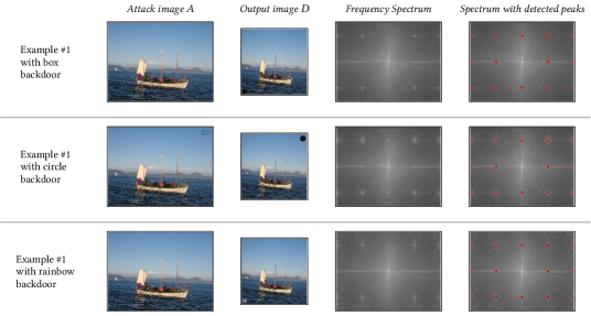
Figure 9. Evaluation examples from backdoor detection. The columns show an attack image, its downscaled version, the frequency spectrum of $A$, and the detected peaks with our frequency method. The first row depicts a scaling attack with a box backdoor in the bottom-left corner. The row in the middle shows an attack with a circle backdoor in the upper-right corner. The last row depicts an attack with the rainbow backdoor in the bottom-left corner. The plots highlight that the frequency traces do not depend on the backdoor’s shape or location.

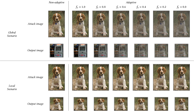
Figure 10. Evaluation examples for the adaptive attack based on suppressing peaks. The first column shows the non-adaptive, original scaling attack, while the further columns show the adaptive modification to bypass the detection. It is visible that small values of $f_{s}$ have a clear impact in the global scenario.

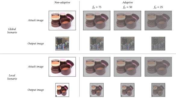
Figure 11. Evaluation examples for the adaptive attack based on adding peaks. The first column shows the non-adaptive, original scaling attack, while the further columns show the adaptive modification to bypass the detection. It is visible that adding peaks reduces the brightness, but the image content remains intact.