Convergence of a steepest descent algorithm in shape optimisation using $W^{1,\infty}$ functions

Abstract

Built upon previous work of the authors in Deckelnick, Herbert, and Hinze, ESAIM: COCV 28 (2022), we present a general shape optimisation framework based on the method of mappings in the $W^{1,\infty}$ topology together with a suitable finite element discretisation. For the numerical solution of the respective discrete shape optimisation problems we propose a steepest descent minimisation algorithm with Armijo-Goldstein stepsize rule. We show that the sequence generated by this descent method globally converges, and under mild assumptions also, that every accumulation point of this sequence is a stationary point of the shape functional. Moreover, for the mesh discretisation parameter tending to zero we under mild assumptions prove convergence of the discrete stationary shapes in the Hausdorff complementary metric. To illustrate our approach we present a selection of numerical examples for PDE constrained shape optimisation problems, where we include numerical convergence studies which support our analytical findings.

Keywords: PDE constrained shape optimisation, $W^{1,\infty}$-steepest-descent, global convergence, finite element discretisation
MSC subject classification: 35Q93, 49Q10, 49J20

1 Introduction

We are interested in the numerical approximation of PDE constrained shape optimisation. Our prototype problem will be of the form

$$\min\mathcal{J}(\Omega):=\int_{\Omega}j(\cdot,u,\nabla u)\,\mathrm{dx},\,\Omega\in\mathcal{S},$$ (1.1)

where $j$ is a real-valued function whose properties will be specified in Section 2 and $u$ weakly solves the Poisson problem

$$-\Delta u=f\text{ in }\Omega,\quad u=0\text{ on }\partial\Omega.$$

Furthermore, $\mathcal{S}$ is a collection of admissible domains contained in a given hold-all domain $D\subset\mathbb{R}^{d}$. We use the method of mappings and assume that each $\Omega\in\mathcal{S}$ is represented by a bi–Lipschitz mapping $\Phi\colon D\rightarrow D$ as $\Omega=\Phi(\hat{\Omega})$, where $\hat{\Omega}\Subset D$ is a fixed reference domain. For domain variations one seeks a mapping $V^{*}\in W^{1,\infty}_{0}(D,\mathbb{R}^{d})$ which forms a descent direction for the shape derivative, i.e. satisfies $\mathcal{J}^{\prime}(\Omega)[V^{*}]<0$. The new domain is then obtained as $\Omega_{\rm new}=({\rm id}+\alpha V^{*})(\Omega)$ with $\alpha>0$ chosen suitably to ensure that the map $\operatorname{id}+\alpha V^{*}$ is bi-Lipschitz. A common approach to determine a descent direction is to work in a Hilbert space $H\hookrightarrow W^{1,\infty}(D,\mathbb{R}^{d})$ and then to find $V^{*}$ as the corresponding Riesz representative of $\mathcal{J}^{\prime}(\Omega)$. Depending on the space dimension this may require the use of Sobolev spaces $H^{m}(D,\mathbb{R}^{d})$ with a larger $m\in\mathbb{N}$ making the discretisation of this approach cumbersome. In this work we follow instead the concept introduced in [DHH22], [DHH23] and suggest to work directly in the space $W^{1,\infty}_{0}(D,\mathbb{R}^{d})$ choosing

$$V^{*}\in\operatorname*{arg\,min}\left\{\mathcal{J}^{\prime}(\Omega)[V]:V\in W^{1,\infty}_{0}(D,\mathbb{R}^{d}),|DV|\leq 1\mbox{ a.e. in }D\right\}$$ (1.2)

as descent direction for the shape minimisation problem. In the above, by $|DV|$, we mean the spectral norm of the matrix $DV$. In order to approximate (1.1) based on this idea we introduce the functional

$$\mathcal{J}_{h}(\Omega_{h}):=\int_{\Omega_{h}}j(\cdot,u_{h},\nabla u_{h})\,\mathrm{dx},\quad\Omega_{h}\in\mathcal{S}_{h},$$ (1.3)

where $u_{h}$ denotes the piecewise linear and continuous finite element function solving the discrete Poisson problem (2.14) and $\mathcal{S}_{h}$ is a suitable approximation of $\mathcal{S}$. For the numerical solution of the discrete shape optimisation problem we propose a steepest descent method with Armijo step size rule which is realised in the $W^{1,\infty}-$ topology as described above. In fact $\mathcal{S}_{h}$ is built upon piecewise linear and continuous approximations $\Phi_{h}$ of the mapping $\Phi$, which in turn are induced by piecewise linear and continuous vector fields $V_{h}^{*}$ solving the discrete counterpart of (1.2). We here note that the use of piecewise linear and continuous finite elements is perfectly tailored to the numerical treatment of our approach, since they belong to $W^{1,\infty}$, and both problems (1.2) and (1.3) can be discretised on the same triangulation $\mathcal{T}_{h}$. It is the purpose of this paper to analyse the resulting numerical method both for a fixed mesh width $h$ and for the case that $h$ tends to zero thereby justifying the underlying approach. The main contributions of this work are

• Theorem 3.3, where global convergence of the steepest descent method is shown for a fixed discretisation parameter, and under mild assumptions also, that every accumulation point of this sequence is a stationary point of the discrete shape functional;

• Theorem 4.4, where it is shown that under suitable conditions a sequence of discrete stationary shapes converges with respect to the Hausdorff complementary metric to a stationary point of (1.1).

An important ingredient in the proof of Theorem 4.4 is the continuity of the Dirichlet problem with respect to the Hausdorff complementary metric which is usually expressed in terms of $\gamma$–convergence or (equivalently) Mosco–convergence. Our analysis is inspired by the work [CZ06] of Chenais and Zuazua, who obtain the convergence of a sequence of discrete minimal shapes, obtained by some finite element approximation, to a minimum of the continuous problem. In [CZ06], Mosco–convergence is a consequence of the assumption that the complementary sets of the discrete optimal shapes have a uniformly bounded number of connected components. In contrast, in our setting it will be more convenient to work with a uniform capacity density condition, see Theorem 4.1. A convergence result for a shape optimisation problem in the class of convex domains has recently been obtained by Bartels and Wachsmuth, [BW20] under a condition that will also appear in our work.
In special settings a priori estimates for finite element approximations of shape optimisation problems have been proved. Here we refer to the works of Kiniger and Vexler [KV13] and Fumagalli et al. [FPV15], where graph settings are considered, and of Eppler et al. [EHS07] for star-shaped domains.
Another aspect that has been examined from the viewpoint of numerical analysis is the approximation of the shape derivative. In [HPS15] Hiptmair, Paganini, and Sargheini study the finite element approximation of the shape derivative under appropriate regularity assumptions of the state and the adjoint state. In [GZ21] Gong and Zhu propose a finite element approximation to the boundary form of the shape derivative in PDE constrained shape optimisation. Zhu and Gao in [ZG19] numerically analyse a mixed finite element approximation of the shape gradient for Stokes flow, and Zhu, Hu and Liao in [ZHL20] provide numerical analysis for the finite element approximation of shape derivatives in eigenvalue optimisation for the Poisson problem. For additional information on the subject of shape optimisation we refer the reader to the seminal works of Delfour and Zolésio [DZ11], of Sokolowski and Zolésio [SZ92], and the recent overview article [ADJ21] by Allaire, Dapogny, and Jouve, where also a comprehensive bibliography on the topic can be found.

Outline:

In Section 2 we provide preliminaries for the formulation and the numerical analysis of our PDE constrained shape optimisation problem. In Section 3 we prove global convergence for the steepest descent method applied to problem (1.3), and in Section 4 prove convergence of discrete stationary points to a stationary point for the limit problem (1.1). In Section 5 we provide numerical experiments which support our theoretical findings.

2 Preliminaries

2.1 Setting of the problem

Let $D\subset\mathbb{R}^{d}$ be an open, convex, polygonal hold-all domain and $\hat{\Omega}\Subset D$ a fixed reference domain. We define

$$\mathcal{U}:=\{\Phi:\bar{D}\rightarrow\bar{D}\,|\,\Phi\mbox{ is a bilipschitz map},\Phi=\mbox{id}\mbox{ on }\partial D\}$$

and our set of admissible shapes as

$$\mathcal{S}:=\{\Omega\subset D\,|\,\Omega=\Phi(\hat{\Omega})\mbox{ for some }\Phi\in\mathcal{U}\}.$$

Let us consider the shape optimisation problem

$$\min_{\Omega\in\mathcal{S}}\mathcal{J}(\Omega)=\int_{\Omega}j(x,u(x),\nabla u(x))\,\mathrm{dx},$$

where $u\in H^{1}_{0}(\Omega)$ is the unique solution of

$$\int_{\Omega}\nabla u\cdot\nabla\eta\,\mathrm{dx}=\langle f,\eta\rangle\qquad\mbox{ for all }\eta\in H^{1}_{0}(\Omega).$$ (2.1)

Our definition of $\mathcal{S}$ allows us to interpret $\mathcal{U}$ as the set of controls for a PDE–constrained optimisation problem. In what follows we assume that $f\in H^{1}(D)$ and that $j\in C^{2}(D\times\mathbb{R}\times\mathbb{R}^{d})$ satisfies

$$|j(x,u,z)|+|j_{x}(x,u,z)|+|j_{xx}(x,u,z)| \leq \varphi_{1}(x)+c_{1}\bigl{(}|u|^{q}+|z|^{2}\bigr{)};$$ (2.2)

$$|j_{u}(x,u,z)|+|j_{xu}(x,u,z)| \leq \varphi_{2}(x)+c_{2}\bigl{(}|u|^{q-1}+|z|^{2-\frac{2}{q}}\bigr{)};$$ (2.3)

$$|j_{z}(x,u,z)|+|j_{xz}(x,u,z)| \leq \varphi_{3}(x)+c_{3}\bigl{(}|u|^{\frac{q}{2}}+|z|\bigr{)};$$ (2.4)

$$|j_{uu}(x,u,z)| \leq \varphi_{4}(x)+c_{4}\bigl{(}|u|^{q-2}+|z|^{2-\frac{4}{q}}\bigr{)};$$ (2.5)

$$|j_{zz}(x,u,z)| \leq \varphi_{5}(x)$$ (2.6)

for all $(x,u,z)\in D\times\mathbb{R}\times\mathbb{R}^{d}$. Here, $2\leq q<\infty$ if $d=2$ and $q=\frac{2d}{d-2}$ if $d\geq 3$. Also, $\varphi_{1},\ldots,\varphi_{5}$ are non-negative with $\varphi_{1}\in L^{1}(D),\varphi_{2}\in L^{\frac{q}{q-1}}(D),\varphi_{3}\in L^{2}(D),\varphi_{4}\in L^{\frac{q}{q-2}}(D)$ and $\varphi_{5}\in L^{\infty}(D)$. Note that the choice of $q$ implies the continuous embedding $H^{1}_{0}(D)\hookrightarrow L^{q}(D)$, so that there exists $c>0$ with

$$\|v\|_{L^{q}}\leq c\|v\|_{H^{1}}\qquad\mbox{ for all }v\in H^{1}_{0}(D).$$ (2.7)

It is well known that the shape derivative of $\mathcal{J}$ is given by

$$\mathcal{J}^{\prime}(\Omega)[V] = \int_{\Omega}\Bigl{(}j(\cdot,u,\nabla u)\operatorname{div}V+j_{x}(\cdot,u,\nabla u)\cdot V-j_{z}(\cdot,u,\nabla u)\cdot DV^{\mathsf{T}}\nabla u\Bigr{)}\,\mathrm{dx}$$

$$+\int_{\Omega}\Bigl{(}\bigl{(}DV+DV^{\mathsf{T}}-\operatorname{div}VI\bigr{)}\nabla u\cdot\nabla p+{\operatorname{div}}(fV)p\Bigr{)}\,\mathrm{dx}$$

for all $V\in W^{1,\infty}_{0}(D,\mathbb{R}^{d})$. Here, $p\in H^{1}_{0}(\Omega)$ is the solution of the adjoint problem

$$\int_{\Omega}\nabla p\cdot\nabla\eta\,\mathrm{dx}=\int_{\Omega}\bigl{(}j_{u}(\cdot,u,\nabla u)\eta+j_{z}(\cdot,u,\nabla u)\cdot\nabla\eta\bigr{)}\,\mathrm{dx}\quad\mbox{ for all }\eta\in H^{1}_{0}(\Omega).$$ (2.9)

We observe that (2.2)–(2.4) together with (2.7) imply that the integrals on the right hand side of (2.1) and (2.9) exist. Finding a global minimiser of $\mathcal{J}$ is usually a very hard task so that numerical methods aim to approximate stationary points, i.e. sets $\Omega\in\mathcal{S}$ that satisfy $\mathcal{J}^{\prime}(\Omega)[V]=0$ for all $V\in W^{1,\infty}_{0}(D,\mathbb{R}^{d})$.

2.2 Discretisation

In order to define a corresponding numerical method we choose an admissible triangulation $\mathcal{\hat{T}}_{h}$ of $\bar{D}$ and define

$$\hat{\mathcal{U}}_{h}:=\{\Phi_{h}\in C^{0}(\bar{D},\mathbb{R}^{d})\,|\,\Phi_{h|\hat{T}}\in P^{1}(\hat{T},\mathbb{R}^{d}),\hat{T}\in\mathcal{\hat{T}}_{h},\Phi_{h}\mbox{ is injective},\Phi_{h}=\mbox{id}\mbox{ on }\partial D\}.$$

We start with the following observation.

Lemma 2.1.

Let $\Phi_{h}\in\hat{\mathcal{U}}_{h}$. Then $\Phi_{h}$ is a bilipschitz map from $\bar{D}$ onto $\bar{D}$.

Proof.

Denoting by deg the Brouwer degree and using that $\Phi_{h}=\mbox{id}$ on $\partial D$, we have for every $p\in D$ that

$$\mbox{deg}(\Phi_{h},D,p)=\mbox{deg}(\mbox{id},D,p)=1.$$

Hence we deduce from the existence property of the degree that there exists $x\in D$ with $p=\Phi_{h}(x)$, and therefore $D\subset\Phi_{h}(D)$. Next we claim that $D$ is closed in $\Phi_{h}(D)$. To see this, let $(p_{n})_{n\in\mathbb{N}}$ be a sequence in $D$ such that $p_{n}\rightarrow p$ as $n\rightarrow\infty$ for some $p\in\Phi_{h}(D)$, say $p=\Phi_{h}(x)$ with $x\in D$. If $p\in\partial D$, then $\Phi_{h}(x)=p=\Phi_{h}(p)$ and hence we obtain in view of the injectivity of $\Phi_{h}$ that $x=p$, a contradiction. Hence $p\in D$. As $D$ is also open in $\Phi_{h}(D)$ and $\Phi_{h}(D)$ is connected we infer that $D=\Phi_{h}(D)$. Recalling again that $\Phi_{h}=\mbox{id}$ on $\partial D$ we see that $\Phi_{h}:\bar{D}\rightarrow\bar{D}$ is bijective. Finally, using the fact that $\Phi_{h}$ is piecewise linear and injective together with the convexity of $D$ it is not difficult to show that there exists a constant $K>1$ depending on $\Phi_{h}$ such that

$$\frac{1}{K}|x-y|\leq|\Phi_{h}(x)-\Phi_{h}(y)|\leq K|x-y|\qquad\forall x,y\in\bar{D}.$$ (2.10)

∎

Similarly as in [BW20, Section 3.2] we shall define our discrete admissible domains via transformations of $\hat{\Omega}$ from the set $\hat{\mathcal{U}}_{h}$. In what follows we assume that $\hat{\Omega}$ is an open polygonal domain such that $\overline{\hat{\Omega}}=\bigcup_{\hat{T}\in\mathcal{\hat{T}}^{\tiny\mbox{ref}}_{h}}\hat{T}\subset D$, where $\mathcal{\hat{T}}^{\tiny\mbox{ref}}_{h}\subset\mathcal{\hat{T}}_{h}$. For later purposes we suppose in addition that $\hat{\Omega}$ satisfies the following exterior corkscrew condition:

$$\exists\lambda\in(0,1)\,\exists s_{0}>0\,\forall\hat{x}\in\partial\hat{\Omega}\,\forall s\in(0,s_{0})\,\exists\hat{y}\in B_{s}(\hat{x}):\quad B_{\lambda s}(\hat{y})\subset B_{s}(\hat{x})\cap\complement\hat{\Omega}.$$ (2.11)

In the above $\complement\hat{\Omega}$ denotes the complement of $\hat{\Omega}$. We then define

$$\mathcal{S}_{h}:=\{\Omega_{h}\subset D\,|\,\Omega_{h}=\Phi_{h}(\hat{\Omega})\mbox{ for some }\Phi_{h}\in\hat{\mathcal{U}}_{h}\}.$$ (2.12)

Note that in view of Lemma 2.1 sets $\Omega_{h}\in\mathcal{S}_{h}$ are triangulated in a natural way via $\mathcal{T}_{\Omega_{h}}=\{\Phi_{h}(\hat{T}),\,\hat{T}\in\mathcal{\hat{T}}^{\tiny\mbox{ref}}_{h}\}$. Given a triangulation of this form we introduce

$$X_{\Omega_{h}}:=\{\eta_{h}\in C^{0}(\overline{\Omega_{h}})\,|\,\eta_{h|T}\in P_{1}(T),T\in\mathcal{T}_{\Omega_{h}},\,\eta_{h}=0\mbox{ on }\partial\Omega_{h}\}.$$

Our discrete shape optimisation problem now reads:

$$\min\mathcal{J}_{h}(\Omega_{h}):=\int_{\Omega_{h}}j(x,u_{h}(x),\nabla u_{h}(x))\,\mathrm{dx},$$ (2.13)

where $u_{h}\in X_{\Omega_{h}}$ is the unique solution of

$$\qquad\int_{\Omega_{h}}\nabla u_{h}\cdot\nabla\eta_{h}\,\mathrm{dx}=\langle f,\eta_{h}\rangle\qquad\mbox{ for all }\eta_{h}\in X_{\Omega_{h}}.$$ (2.14)

We remark that we have chosen linear finite elements merely for convenience and that one may take any conforming finite element space in order to approximate the solution of (2.1).
Let us fix $\Omega_{h}=\Phi_{h}(\hat{\Omega})\in\mathcal{S}_{h}$ for some $\Phi_{h}\in\hat{\mathcal{U}}_{h}$. In order to define a suitable perturbation of $\Omega_{h}$ we let

$$\mathcal{V}_{\Phi_{h}}:=\{V_{h}\in C^{0}(\bar{D},\mathbb{R}^{d})\,|\,V_{h|T}\in P_{1}(T,\mathbb{R}^{d}),T=\Phi_{h}(\hat{T}),\hat{T}\in\mathcal{\hat{T}}_{h},\,V_{h}=0\mbox{ on }\partial D\}.$$ (2.15)

Suppose that $V_{h}\in\mathcal{V}_{\Phi_{h}}$ with $|DV_{h}|\leq 1$ in $\bar{D}$. Clearly, $\Phi_{h}+tV_{h}\circ\Phi_{h}$ belongs to $\hat{\mathcal{U}}_{h}$ provided that $|t|<1$. Hence $\Omega_{h,t}:=(\mbox{id}+tV_{h})(\Omega_{h})=(\Phi_{h}+tV_{h}\circ\Phi_{h})(\hat{\Omega})\in\mathcal{S}_{h}$ if $|t|<1$ and we may define $\displaystyle\mathcal{J}_{h}^{\prime}(\Omega_{h})[V_{h}]:=\frac{d}{dt}\mathcal{J}_{h}(\Omega_{h,t})_{|t=0}$. The formula for $\mathcal{J}^{\prime}(\Omega_{h})[V_{h}]$ is obtained analogously to the continuous case. As the corresponding arguments will appear in the proof of Lemma 3.2 below we here merely state its form:

$$\mathcal{J}_{h}^{\prime}(\Omega_{h})[V_{h}] = \int_{\Omega_{h}}\Bigl{(}j(\cdot,u_{h},\nabla u_{h}){\operatorname{div}}V_{h}+j_{x}(\cdot,u_{h},\nabla u_{h})\cdot V_{h}-j_{z}(\cdot,u_{h},\nabla u_{h})\cdot DV_{h}^{\mathsf{T}}\nabla u_{h}\Bigr{)}\,\mathrm{dx}$$ (2.16)

$$+\int_{\Omega_{h}}\Bigl{(}\bigl{(}DV_{h}+DV_{h}^{\mathsf{T}}-{\operatorname{div}}V_{h}I\bigr{)}\nabla u_{h}\cdot\nabla p_{h}+{\operatorname{div}}(fV_{h})p_{h}\Bigr{)}\,\mathrm{dx},$$

where $p_{h}\in X_{\Omega_{h}}$ solves

$$\int_{\Omega_{h}}\nabla p_{h}\cdot\nabla\eta_{h}\,\mathrm{dx}=\int_{\Omega_{h}}\bigl{(}j_{u}(\cdot,u_{h},\nabla u_{h})\eta_{h}+j_{z}(\cdot,u_{h},\nabla u_{h})\cdot\nabla\eta_{h}\bigr{)}\,\mathrm{dx}\quad\mbox{ for all }\eta_{h}\in X_{\Omega_{h}}.$$ (2.17)

2.3 Descent algorithm

With the notation introduced in the previous section we may now formulate a steepest descent method with Armijo search:

Algorithm 2.1 (Steepest descent).

0. Let $\Omega^{0}_{h}:=\hat{\Omega},\Phi^{0}_{h}=\operatorname{id}$.
For k=0,1,2,…:
1. If $\mathcal{J}_{h}^{\prime}(\Omega^{k}_{h})=0$, then stop.
2. Choose $V^{k}_{h}\in\mathcal{V}_{\Phi^{k}_{h}}$ such that

$$V^{k}_{h}=\operatorname*{arg\,min}\{J_{h}^{\prime}(\Omega^{k}_{h})[W_{h}]\,|\,W_{h}\in\mathcal{V}_{\Phi^{k}_{h}},\,|DW_{h}|\leq 1\mbox{ in }\bar{D}\}.$$

3. Choose the maximum $t_{k}\in\{\frac{1}{2},\frac{1}{4},\ldots\}$ such that

$$\mathcal{J}_{h}\bigl{(}(\operatorname{id}+t_{k}V^{k}_{h})(\Omega^{k}_{h})\bigr{)}-\mathcal{J}_{h}(\Omega^{k}_{h})\leq\gamma t_{k}\mathcal{J}_{h}^{\prime}(\Omega^{k}_{h})[V^{k}_{h}].$$

4. Set $\Phi_{h}^{k+1}:=(\mbox{id}+t_{k}V_{h}^{k})\circ\Phi_{h}^{k},\,\Omega^{k+1}_{h}:=(\mbox{id}+t_{k}V^{k}_{h})(\Omega^{k}_{h})$.

Here, $\gamma\in(0,1)$ is a fixed constant. In view of the remarks after (2.15) the algorithm produces a sequence $(\Phi_{h}^{k})_{k\in\mathbb{N}_{0}}\subset\hat{\mathcal{U}}_{h}$ such that $\Omega_{h}^{k}=\Phi_{h}^{k}(\hat{\Omega})\in\mathcal{S}_{h},k\in\mathbb{N}_{0}$. Our aim is to show that

$$\|\mathcal{J}_{h}^{\prime}(\Omega^{k}_{h})\|:=\sup\{\mathcal{J}_{h}^{\prime}(\Omega^{k}_{h})[W_{h}]\,|\,W_{h}\in\mathcal{V}_{\Phi^{k}_{h}},|DW_{h}|\leq 1\mbox{ in }\bar{D}\}\rightarrow 0,\quad\mbox{ as }k\rightarrow\infty.$$

3 Convergence of the descent algorithm

In the present section we investigate the global convergence of the descent Algorithm (2.1), where the discretisation parameter $h$ is kept fixed. As a first step we note the following a–priori bounds on the discrete state and its adjoint state.

Lemma 3.1.

Let $\Omega_{h}=\Phi_{h}(\hat{\Omega})\in\mathcal{S}_{h}$ and $u_{h},p_{h}\in X_{\Omega_{h}}$ the solutions of (2.14), (2.17) respectively. Then

$$\|u_{h}\|_{H^{1}}\leq c\|f\|_{L^{2}},\quad\|p_{h}\|_{H^{1}}\leq c\bigl{(}1+\|f\|_{L^{2}}^{q-1}\bigr{)},$$ (3.1)

where the constant $c$ only depends on $d,j$ and $D$. Here we think of $u_{h}$ and $p_{h}$ as being extended by zero to $D$.

Proof.

The first estimate is standard. In order to prove the bound on $p_{h}$ we test (2.17) with $\eta_{h}=p_{h}\in X_{\Omega_{h}}$ and use (2.3), (2.4), Hölder’s inequality and (2.7) to obtain

$$\int_{D}|\nabla p_{h}|^{2}\,\mathrm{dx}=\int_{\Omega_{h}}|\nabla p_{h}|^{2}\,\mathrm{dx}$$

$$\leq \int_{\Omega_{h}}\left[\bigl{(}\varphi_{2}+c_{2}(|u_{h}|^{q-1}+|\nabla u_{h}|^{\frac{2(q-1)}{q}})\bigr{)}|p_{h}|+\bigl{(}\varphi_{3}+c_{3}(|u_{h}|^{\frac{q}{2}}+|\nabla u_{h}|)\bigr{)}|\nabla p_{h}|\right]\,\mathrm{dx}$$

$$\leq \bigl{(}\|\varphi_{2}\|_{L^{\frac{q}{q-1}}}+c_{2}(\|u_{h}\|_{L^{q}}^{q-1}+\|\nabla u_{h}\|_{L^{2}}^{\frac{2(q-1)}{q}})\bigr{)}\|p_{h}\|_{L^{q}}$$

$$+\bigl{(}\|\varphi_{3}\|_{L^{2}}+c_{3}(\|u_{h}\|_{L^{q}}^{\frac{q}{2}}+\|\nabla u_{h}\|_{L^{2}})\bigr{)}\|\nabla p_{h}\|_{L^{2}}$$

$$\leq c\bigl{(}1+\|u_{h}\|_{H^{1}}^{q-1}\bigr{)}\|p_{h}\|_{H^{1}}\leq c\bigl{(}1+\|f\|_{L^{2}}^{q-1}\bigr{)}\|p_{h}\|_{H^{1}}\leq c\bigl{(}1+\|f\|_{L^{q}}^{q-1}\bigr{)}\|\nabla p_{h}\|_{L^{2}},$$

where we also made use of Poincaré’s inequality for $D$ and the bound on $u_{h}$. The estimate for $\|p_{h}\|_{L^{2}}$ now follows from another application of Poincaré’s inequality. ∎

In order to establish the convergence of $\mathcal{J}_{h}^{\prime}(\Omega^{k}_{h})$ we follow the general procedure outlined in Section 2.2.1 of [Hin+08]. The following result can be seen as an analogue of Lemma 2.2 in [Hin+08], where the uniform continuity of the derivative of the objective functional that is assumed in that result needs to be replaced by suitable arguments.

Lemma 3.2.

Let $\Omega_{h}=\Phi_{h}(\hat{\Omega})\in\mathcal{S}_{h},\,\mathcal{V}_{\Phi_{h}}$ as in (2.15) and $V_{h}\in\mathcal{V}_{\Phi_{h}}$ such that

$$V_{h}=\operatorname*{arg\,min}\{J_{h}^{\prime}(\Omega_{h})[W_{h}]\,|\,W_{h}\in\mathcal{V}_{\Phi_{h},}\,|DW_{h}|\leq 1\mbox{ in }\bar{D}\}.$$

Suppose that $\mathcal{J}_{h}^{\prime}(\Omega_{h})[V_{h}]\leq-\epsilon$ for some $\epsilon>0$. Then there exists $0<\delta<1$ which only depends on $j,f,D,d,\gamma$ and $\epsilon$ such that

$$\mathcal{J}_{h}(\Omega_{h,t})-\mathcal{J}_{h}(\Omega_{h})\leq\gamma t\mathcal{J}_{h}^{\prime}(\Omega_{h})[V_{h}]\qquad\mbox{ for all }0\leq t\leq\delta,$$

where $\Omega_{h,t}=T_{t}(\Omega_{h})$ and $T_{t}=\mbox{id}+tV_{h}$.

Proof.

We follow the standard procedure for calculating the shape derivative with special attention on controlling the remainder terms. Recalling the definition of $\mathcal{J}_{h}$ we have

$$\mathcal{J}_{h}(\Omega_{h,t})=\int_{\Omega_{h,t}}j(\cdot,u_{h,t},\nabla u_{h,t})\,\mathrm{dx},$$

where $u_{h,t}\in X_{\Omega_{h,t}}$ solves

$$\int_{\Omega_{h,t}}\nabla u_{h,t}\cdot\nabla\eta_{h,t}\,\mathrm{dx}=\int_{\Omega_{h,t}}f\eta_{h,t}\,\mathrm{dx}\qquad\forall\eta_{h,t}\in X_{\Omega_{h,t}}.$$

For $\eta_{h}\in X_{\Omega_{h}}$ we have that $\eta_{h,t}:=\eta_{h}\circ T_{t}^{-1}\in X_{\Omega_{h,t}}$ and hence

$$\int_{\Omega_{h,t}}\nabla u_{h,t}\cdot\nabla(\eta_{h}\circ T_{t}^{-1})\,\mathrm{dx}=\int_{\Omega_{h,t}}f\eta_{h}\circ T_{t}^{-1}\,\mathrm{dx}\qquad\forall\eta_{h}\in X_{\Omega_{h}},$$ (3.2)

from which we infer with the help of the transformation rule

$$\int_{\Omega_{h}}\nabla u_{h,t}\circ T_{t}\cdot\nabla(\eta_{h}\circ T_{t}^{-1})\circ T_{t}\,|\mbox{det}DT_{t}|\,\mathrm{dx}=\int_{\Omega_{h}}f\circ T_{t}\,\eta_{h}\,|\mbox{det}DT_{t}|\,\mathrm{dx}\qquad\forall\eta_{h}\in X_{\Omega_{h}}.$$ (3.3)

Since $|DV_{h}|\leq 1$ in $\bar{D}$ we have

$$\mbox{det}DT_{t}-1=t{\operatorname{div}}V_{h}+r_{1},\quad\mbox{ with }|r_{1}|\leq ct^{2},$$ (3.4)

where the constant $c$ only depends on $d$. In particular there is $\delta_{1}>0$ so that $\mbox{det}DT_{t}>0,0\leq t\leq\delta_{1}$. If we define $\hat{u}_{h,t}:=u_{h,t}\circ T_{t}\in X_{\Omega_{h}}$ and $A_{t}:=(DT_{t})^{-1}(DT_{t})^{-\mathsf{T}}\mbox{det}DT_{t}$ the relation (3.3) can be written in the form

$$\int_{\Omega_{h}}A_{t}\nabla\hat{u}_{h,t}\cdot\nabla\eta_{h}\,\mathrm{dx}=\int_{\Omega_{h}}f\circ T_{t}\,\eta_{h}\,\mbox{det}DT_{t}\,\mathrm{dx}\qquad\mbox{ for all }\eta_{h}\in X_{\Omega_{h}}.$$ (3.5)

Thus we have

$$\mathcal{J}_{h}(\Omega_{h,t})-\mathcal{J}_{h}(\Omega_{h})$$ (3.6)

$$= \int_{\Omega_{h}}\bigl{(}j(T_{t},\hat{u}_{h,t},DT_{t}^{-\mathsf{T}}\nabla\hat{u}_{h,t})\,\mbox{det}DT_{t}-j(\cdot,u_{h},\nabla u_{h})\bigr{)}\,\mathrm{dx}$$

$$= \int_{\Omega_{h}}j(\cdot,u_{h},\nabla u_{h})(\mbox{det}DT_{t}-1)\,\mathrm{dx}+\int_{\Omega_{h}}\bigl{(}j(T_{t},\hat{u}_{h,t},DT_{t}^{-\mathsf{T}}\nabla\hat{u}_{h,t})-j(\cdot,u_{h},\nabla u_{h})\bigr{)}\,\mathrm{dx}$$

$$+\int_{\Omega_{h}}\bigl{(}j(T_{t},\hat{u}_{h,t},DT_{t}^{-\mathsf{T}}\nabla\hat{u}_{h,t})-j(\cdot,u_{h},\nabla u_{h})\bigr{)}(\mbox{det}DT_{t}-1)\,\mathrm{dx}$$

$$= \sum_{j=1}^{3}T_{j}.$$

We deduce with the help of (3.4), (2.2), (2.7) and (3.1) that

$$T_{1}=t\int_{\Omega_{h}}j(\cdot,u_{h},\nabla u_{h})\operatorname{div}V_{h}\,\mathrm{dx}+\int_{\Omega_{h}}j(\cdot,u_{h},\nabla u_{h})\,r_{1}\,\mathrm{dx}$$ (3.7)

$$\leq t\int_{\Omega_{h}}j(\cdot,u_{h},\nabla u_{h})\operatorname{div}V_{h}\,\mathrm{dx}+ct^{2}\int_{\Omega_{h}}(\varphi_{1}+c_{1}|u_{h}|^{q}+c_{1}|\nabla u_{h}|^{2})\,\mathrm{dx}$$

$$\leq t\int_{\Omega_{h}}j(\cdot,u_{h},\nabla u_{h})\operatorname{div}V_{h}\,\mathrm{dx}+ct^{2}\bigl{(}1+\|u_{h}\|_{H^{1}}^{q}\bigr{)}\leq t\int_{\Omega_{h}}j(\cdot,u_{h},\nabla u_{h})\operatorname{div}V_{h}\,\mathrm{dx}+ct^{2}.$$

In order to treat $T_{2}$ we use Taylor’s formula and write

$$j(T_{t},\hat{u}_{h,t},DT_{t}^{-\mathsf{T}}\nabla\hat{u}_{h,t})-j(\cdot,u_{h},\nabla u_{h})$$

$$= tj_{x}()\cdot V_{h}+j_{u}()(\hat{u}_{h,t}-u_{h})+j_{z}()\cdot(DT_{t}^{-\mathsf{T}}\nabla\hat{u}_{h,t}-\nabla u_{h})$$

$$+\int_{0}^{1}(1-s)\frac{d^{2}}{ds^{2}}\left[j(\cdot+stV_{h},s\hat{u}_{h,t}+(1-s)u_{h},sDT_{t}^{-\mathsf{T}}\nabla\hat{u}_{h,t}+(1-s)\nabla u_{h})\right]ds,$$

where the first order derivatives of $j$ are evaluated at $(\cdot,u_{h},\nabla u_{h})$. Thus we have

$$T_{2} = t\int_{\Omega_{h}}j_{x}(\cdot,u_{h},\nabla u_{h})\cdot V_{h}\,\mathrm{dx}-t\int_{\Omega_{h}}j_{z}(\cdot,u_{h},\nabla u_{h})\cdot DV_{h}^{\mathsf{T}}\nabla u_{h}$$ (3.8)

$$+\int_{\Omega_{h}}j_{z}(\cdot,u_{h},\nabla u_{h})\cdot\bigl{(}(DT_{t}^{-\mathsf{T}}-I+tDV_{h}^{\mathsf{T}})\nabla\hat{u}_{h,t}+tDV_{h}^{\mathsf{T}}\nabla(u_{h}-\hat{u}_{h,t})\bigr{)}\,\mathrm{dx}$$

$$+\int_{\Omega_{h}}\bigl{(}j_{u}(\cdot,u_{h},\nabla u_{h})(\hat{u}_{h,t}-u_{h})+j_{z}(\cdot,u_{h},\nabla u_{h})\cdot\nabla(\hat{u}_{h,t}-u_{h})\bigr{)}\,\mathrm{dx}$$

$$+\int_{\Omega_{h}}\int_{0}^{1}(1-s)\frac{d^{2}}{ds^{2}}\left[j(\cdot+stV_{h},s\hat{u}_{h,t}+(1-s)u_{h},sDT_{t}^{-\mathsf{T}}\nabla\hat{u}_{h,t}+(1-s)\nabla u_{h})\right]ds\,\mathrm{dx}$$

$$= \sum_{j=1}^{5}T_{2,j}.$$

Let us begin with the term $T_{2,3}$. Observing that $DT_{t}^{-\mathsf{T}}=(I+tDV_{h})^{-\mathsf{T}}=I-tDV_{h}^{\mathsf{T}}+R_{2}$ with $|R_{2}|\leq ct^{2}$ we deduce with the help of Hölder’s inequality, (2.4), (2.7) and (3.1)

$$T_{2,3} \leq \int_{\Omega_{h}}|j_{z}(\cdot,u_{h},\nabla u_{h})|\bigl{(}|R_{2}|\,|\nabla\hat{u}_{h,t}|+t\,|\nabla(\hat{u}_{h,t}-u_{h})|\bigr{)}\,\mathrm{dx}$$ (3.9)

$$\leq c\bigl{(}\|\varphi_{3}\|_{L^{2}}+\|u_{h}\|_{L^{q}}^{\frac{q}{2}}+\|\nabla u_{h}\|_{L^{2}}\bigr{)}\bigl{(}t^{2}\|\hat{u}_{h,t}\|_{H^{1}}+t\|\hat{u}_{h,t}-u_{h}\|_{H^{1}}\bigr{)}$$

$$\leq c\bigl{(}1+\|u_{h}\|_{H^{1}}^{\frac{q}{2}}\bigr{)}\bigl{(}t^{2}+c\|\hat{u}_{h,t}-u_{h}\|_{H^{1}}^{2}\bigr{)}\leq c\bigl{(}t^{2}+c\|\hat{u}_{h,t}-u_{h}\|_{H^{1}}^{2}\bigr{)}.$$

Next, using (2.17), (2.14) and (3.5) we obtain

$$T_{2,4} = \int_{\Omega_{h}}\nabla p_{h}\cdot\nabla(\hat{u}_{h,t}-u_{h})\,\mathrm{dx}=\int_{\Omega_{h}}\nabla p_{h}\cdot\nabla\hat{u}_{h,t}\,\mathrm{dx}-\int_{\Omega_{h}}\nabla p_{h}\cdot\nabla u_{h}\,\mathrm{dx}$$

$$= \int_{\Omega_{h}}(I-A_{t})\nabla p_{h}\cdot\nabla u_{h}\,\mathrm{dx}+\int_{\Omega_{h}}(I-A_{t})\nabla p_{h}\cdot\nabla(\hat{u}_{h,t}-u_{h})\,\mathrm{dx}$$

$$+\int_{\Omega_{h}}\bigl{(}f\circ T_{t}\,\mbox{det}DT_{t}-f\bigr{)}p_{h}\,\mathrm{dx}=\sum_{k=1}^{3}\tilde{T}_{k}.$$

Recalling that $A_{t}=(DT_{t})^{-1}(DT_{t})^{-\mathsf{T}}\mbox{det}DT_{t}$ it is not difficult to see that

$$I-A_{t}=t\bigl{(}DV_{h}+DV_{h}^{\mathsf{T}}-\operatorname{div}V_{h}I\bigr{)}+R_{3},\qquad\mbox{ with }|R_{3}|\leq ct^{2},$$ (3.10)

where $c$ only depends on $d$. Hence

$$\tilde{T}_{1} = t\int_{\Omega_{h}}\bigl{(}DV_{h}+DV_{h}^{\mathsf{T}}-\operatorname{div}V_{h}I\bigr{)}\nabla u_{h}\cdot\nabla p_{h}\,\mathrm{dx}+\int_{\Omega_{h}}R_{3}\nabla u_{h}\cdot\nabla p_{h}\,\mathrm{dx}$$ (3.11)

$$\leq t\int_{\Omega_{h}}\bigl{(}DV_{h}+DV_{h}^{\mathsf{T}}-\operatorname{div}V_{h}I\bigr{)}\nabla u_{h}\cdot\nabla p_{h}\,\mathrm{dx}+ct^{2}$$

in view of (3.1). Next

$$\tilde{T}_{2}\leq ct\|\nabla p_{h}\|_{L^{2}}\|\nabla(\hat{u}_{h,t}-u_{h})\|_{L^{2}}\leq ct\|\nabla(\hat{u}_{h,t}-u_{h})\|_{L^{2}}$$ (3.12)

again by (3.1). In order to deal with $\tilde{T}_{3}$ we write for $x\in\Omega_{h}$

$$f(T_{t}(x))=f(x)+t\int_{0}^{1}\nabla f(x+stV_{h}(x))\cdot V_{h}(x)\,\mathrm{ds},$$

which, combined with (3.4) yields

$$f\circ T_{t}\,\mbox{det}DT_{t}-f = (f\circ T_{t}-f)+tf\circ T_{t}\,\operatorname{div}V_{h}+r_{1}f\circ T_{t}$$

$$= t\nabla f\cdot V_{h}+tf\operatorname{div}V_{h}+t\int_{0}^{1}\bigl{(}\nabla f(\cdot+stV_{h})-\nabla f\bigr{)}\cdot V_{h}\,\mathrm{ds}$$

$$+t^{2}\int_{0}^{1}\nabla f(\cdot+stV_{h})\cdot V_{h}\,\mathrm{ds}\,\operatorname{div}V_{h}+r_{1}f\circ T_{t}.$$

This implies together with (3.4) and (3.1)

$$\tilde{T}_{3} \leq t\int_{\Omega_{h}}\operatorname{div}(fV_{h})p_{h}\,\mathrm{dx}+ct^{2}\|p_{h}\|_{L^{2}}\|f\|_{H^{1}}+ct\|p_{h}\|_{L^{2}}\sup_{0\leq\sigma\leq t}\|\nabla f\circ T_{\sigma}-\nabla f\|_{L^{2}}$$ (3.14)

$$\leq t\int_{\Omega_{h}}\operatorname{div}(fV_{h})p_{h}\,\mathrm{dx}+ct^{2}+ct\sup_{0\leq\sigma\leq t}\|\nabla f\circ T_{\sigma}-\nabla f\|_{L^{2}}.$$

Here we have also used that

$$|V_{h}(x)|\leq\mbox{diam}(D)\sup_{y\in D}|DV_{h}(y)|\leq\mbox{diam}(D),\;x\in D,$$ (3.15)

since $V_{h}=0$ on $\partial D$ and $|DV_{h}|\leq 1$ in $D$. Collecting the above terms we have

$$T_{2,4} \leq t\int_{\Omega_{h}}\bigl{(}DV_{h}+DV_{h}^{\mathsf{T}}-\operatorname{div}V_{h}I\bigr{)}\nabla u_{h}\cdot\nabla p_{h}\,\mathrm{dx}+t\int_{\Omega_{h}}\operatorname{div}(fV_{h})p_{h}\,\mathrm{dx}$$ (3.16)

$$+ct^{2}+c\|\hat{u}_{h,t}-u\|_{H^{1}}^{2}+ct\sup_{0\leq\sigma\leq t}\|\nabla f\circ T_{\sigma}-\nabla f\|_{L^{2}}.$$

Finally, the term $T_{2,5}$ involves a sum of products of second order partial derivatives of $j$ with $tV_{h},\hat{u}_{h,t}-u_{h}$ and $DT_{t}^{-\mathsf{T}}\nabla\hat{u}_{h,t}-\nabla u_{h}$. By way of example we use (2.4) to estimate for $0\leq s\leq 1$

$$\int_{\Omega_{h}}|j_{xz}(\cdot+stV_{h},s\hat{u}_{h,t}+(1-s)u_{h},sDT_{t}^{-\mathsf{T}}\nabla\hat{u}_{h,t}+(1-s)\nabla u_{h})|\,t\,|V_{h}|\,|DT_{t}^{-\mathsf{T}}\nabla\hat{u}_{h,t}-\nabla u_{h}|\,\mathrm{dx}$$

$$\leq t\|V_{h}\|_{L^{\infty}}\int_{\Omega_{h}}\bigl{(}\varphi_{3}\circ(\mbox{id}+stV_{h})+|s\hat{u}_{h,t}+(1-s)u_{h}|^{\frac{q}{2}}$$

$$\qquad\qquad\quad\quad+|sDT_{t}^{-\mathsf{T}}\nabla\hat{u}_{h,t}+(1-s)\nabla u_{h}|\bigr{)}|DT_{t}^{-\mathsf{T}}\nabla\hat{u}_{h,t}-\nabla u_{h}|\,\mathrm{dx}$$

$$\leq ct\bigl{(}\|\varphi_{3}\|_{L^{2}}+\|\hat{u}_{h,t}\|_{L^{q}}^{\frac{q}{2}}+\|u_{h}\|_{L^{q}}^{\frac{q}{2}}+\|\nabla\hat{u}_{h,t}\|_{L^{2}}+\|\nabla u_{h}\|_{L^{2}}\bigr{)}\|DT_{t}^{-\mathsf{T}}\nabla\hat{u}_{h,t}-\nabla u_{h}\|_{L^{2}}$$

$$\leq ct\bigl{(}1+\|\hat{u}_{h,t}\|_{H^{1}}^{\frac{q}{2}}+\|u_{h}\|_{H^{1}}^{\frac{q}{2}}\bigr{)}\bigl{(}\|DT_{t}^{-\mathsf{T}}-I\|_{L^{\infty}}\|\hat{u}_{h,t}\|_{H^{1}}+\|\hat{u}_{h,t}-u_{h}\|_{H^{1}}\bigr{)}$$

$$\leq ct\bigl{(}t+\|\hat{u}_{h,t}-u_{h}\|_{H^{1}}\bigr{)}\leq ct^{2}+c\|\hat{u}_{h,t}-u_{h}\|_{H^{1}}^{2}.$$

Arguing in a similar way for the other terms we obtain

$$T_{2,5}\leq ct^{2}+c\|\hat{u}_{h,t}-u_{h}\|_{H^{1}}^{2},$$ (3.17)

so that in conclusion

$$T_{2} \leq t\int_{\Omega_{h}}j_{x}(\cdot,u_{h},\nabla u_{h})\cdot V_{h}\,\mathrm{dx}-t\int_{\Omega_{h}}j_{z}(\cdot,u_{h},\nabla u_{h})\cdot DV_{h}^{\mathsf{T}}\nabla u_{h}$$ (3.18)

$$+t\int_{\Omega_{h}}\bigl{(}DV_{h}+DV_{h}^{\mathsf{T}}-\operatorname{div}V_{h}I\bigr{)}\nabla u_{h}\cdot\nabla p_{h}\,\mathrm{dx}+t\int_{\Omega_{h}}\operatorname{div}(fV_{h})p_{h}\,\mathrm{dx}$$

$$+ct^{2}+c\|\hat{u}_{h,t}-u_{h}\|_{H^{1}}^{2}+ct\sup_{0\leq\sigma\leq t}\|\nabla f\circ T_{\sigma}-\nabla f\|_{L^{2}}.$$

In order to treat $T_{3}$ we write

$$j(T_{t},\hat{u}_{h,t},DT_{t}^{-\mathsf{T}}\nabla\hat{u}_{h,t})-j(\cdot,u_{h},\nabla u_{h})$$

$$= \int_{0}^{1}\frac{d}{ds}j(\cdot+stV_{h},s\hat{u}_{h,t}+(1-s)u_{h},sDT_{t}^{-\mathsf{T}}\nabla\hat{u}_{h,t}+(1-s)\nabla u_{h})ds,$$

use the growth assumptions on $j_{x},j_{u},j_{z}$ as well as (3.4) and derive

$$T_{3}\leq ct\bigl{(}t+\|\hat{u}_{h,t}-u_{h}\|_{H^{1}}\bigr{)}\leq ct^{2}+c\|\hat{u}_{h,t}-u_{h}\|_{H^{1}}^{2}.$$ (3.19)

If we insert the estimates (3.7), (3.18) and (3.19) into (3.6) and recall (2.16) we obtain

$$\mathcal{J}_{h}(\Omega_{h,t})-\mathcal{J}_{h}(\Omega_{h})\leq t\mathcal{J}_{h}^{\prime}(\Omega_{h})[V_{h}]+ct\bigl{(}t+\sup_{0\leq\sigma\leq t}\|\nabla f\circ T_{\sigma}-\nabla f\|_{L^{2}}\bigr{)}+c\|\hat{u}_{h,t}-u_{h}\|^{2}_{H^{1}}.$$ (3.20)

In order to estimate $\|\hat{u}_{h,t}-u_{h}\|_{H^{1}}$ we combine (2.14) and (3.5) to obtain

$$\int_{\Omega_{h}}A_{t}\nabla(\hat{u}_{h,t}-u_{h})\cdot\nabla\eta_{h}\,\mathrm{dx}=\int_{\Omega_{h}}(I-A_{t})\nabla u_{h}\cdot\nabla\eta_{h}\,\mathrm{dx}+\int_{\Omega_{h}}\bigl{(}f\circ T_{t}\,\mbox{det}DT_{t}-f\bigr{)}\eta_{h}\,\mathrm{dx}\qquad\forall\eta_{h}\in X_{\Omega_{h}}.$$

In view of (3.10) there exists $0<\delta_{2}\leq\delta_{1}$ such that $A_{t}\xi\cdot\xi\geq\frac{1}{2}|\xi|^{2}$ for all $\xi\in\mathbb{R}^{d}$ and $0\leq t\leq\delta_{2}$. Inserting $\eta_{h}=\hat{u}_{h,t}-u_{h}$ into the above relation and using (3.10) as well as (3) we infer with the help of Poincaré’s inequality that

$$\frac{1}{2}\int_{D}|\nabla(\hat{u}_{h,t}-u_{h})|^{2}\,\mathrm{dx} \leq ct\|\nabla u_{h}\|_{L^{2}}\|\nabla(\hat{u}_{h,t}-u_{h})\|_{L^{2}}+ct\|f\|_{H^{1}}\|\hat{u}_{h,t}-u_{h}\|_{L^{2}}$$

$$\leq \frac{1}{4}\|\nabla(\hat{u}_{h,t}-u_{h})\|_{L^{2}}^{2}+ct^{2},$$

from which we deduce that $\|\hat{u}_{h,t}-u_{h}\|_{H^{1}}\leq ct$. If we insert this bound into (3.20) and use that $\mathcal{J}_{h}^{\prime}(\Omega_{h})[V_{h}]\leq-\epsilon$ we obtain

$$\mathcal{J}_{h}(\Omega_{h,t})-\mathcal{J}_{h}(\Omega_{h})\leq t\mathcal{J}_{h}^{\prime}(\Omega_{h})[V_{h}]+ct\bigl{(}t+\sup_{0\leq\sigma\leq t}\|\nabla f\circ T_{\sigma}-\nabla f\|_{L^{2}}\bigr{)}$$ (3.21)

$$\leq \gamma t\mathcal{J}_{h}^{\prime}(\Omega_{h})[V_{h}]+ct\bigl{(}t+\sup_{0\leq\sigma\leq t}\|\nabla f\circ T_{\sigma}-\nabla f\|_{L^{2}}\bigr{)}-(1-\gamma)\epsilon t.$$

There exists $0<\delta\leq\delta_{2}$ such that $\sup_{0\leq\sigma\leq t}\|\nabla f\circ T_{\sigma}-\nabla f\|_{L^{2}}\leq\frac{1}{2c}(1-\gamma)\epsilon$ for $0\leq t\leq\delta$. This can be seen as usual by approximating $f_{x_{i}}$ by a continuous function $g_{i}$, using the uniform continuity of $g_{i}$ on $\bar{D}$ and noting that by (3.15)

$$|T_{\sigma}(x)-x|=\sigma|V_{h}(x)|\leq\mbox{diam}(D)t,\quad 0\leq\sigma\leq t,\,x\in D.$$

By choosing $\delta$ smaller if necessary we can achieve in addition that $\delta\leq\frac{1}{2c}(1-\gamma)\epsilon$. Inserting these bounds into (3.21) we obtain the result of the theorem. ∎

We are now in position to prove our first convergence result.

Theorem 3.3.

Let $(\Phi_{h}^{k})_{k\in\mathbb{N}_{0}}\subset\hat{\mathcal{U}}_{h}$ and $(\Omega^{k}_{h}=\Phi^{k}_{h}(\hat{\Omega}))_{k\in\mathbb{N}_{0}}\subset\mathcal{S}_{h}$ be the sequences generated by Algorithm 2.1. Then:
(i) $\|\mathcal{J}_{h}^{\prime}(\Omega^{k}_{h})\|\rightarrow 0$ as $k\rightarrow\infty$.
(ii) If $\sup_{k\in\mathbb{N}_{0}}|(D\Phi^{k}_{h})^{-1}|\leq C$, then there exists a subsequence $(\Phi^{k_{\ell}}_{h})_{\ell\in\mathbb{N}}$, which converges in $W^{1,\infty}(D)$ to a mapping $\Phi_{h}\in\hat{\mathcal{U}}_{h}$ and $\Omega_{h}:=\Phi_{h}(\hat{\Omega})$ is a stationary point of $\mathcal{J}_{h}$, i.e. satisfies $\mathcal{J}_{h}^{\prime}(\Omega_{h})[V_{h}]=0$ for all $V_{h}\in\mathcal{V}_{\Phi_{h}}$.

Proof.

(i) Since $\mathcal{J}_{h}(\Omega^{k+1}_{h})\leq\mathcal{J}_{h}(\Omega^{k}_{h})$ and

$$\mathcal{J}_{h}(\Omega^{k}_{h}) \geq -\int_{\Omega^{k}_{h}}|j(\cdot,u^{k}_{h},\nabla u^{k}_{h})|\,\mathrm{dx}\geq-\int_{\Omega^{k}_{h}}(\varphi_{1}+c_{1}\bigl{(}|u^{k}_{h}|^{q}+|\nabla u^{k}_{h}|^{2}\bigr{)}\,\mathrm{dx}$$

$$\geq -c\bigl{(}1+\|u^{k}_{h}\|^{q}_{H^{1}}\bigr{)}\geq-c,$$

we infer that $\lim_{k\rightarrow\infty}\mathcal{J}_{h}(\Omega^{k}_{h})=:\beta\in\mathbb{R}$ exists. Then

$$\sum_{k=0}^{\infty}\bigl{(}\mathcal{J}_{h}(\Omega^{k}_{h})-\mathcal{J}_{h}(\Omega^{k+1}_{h})\bigr{)}=\mathcal{J}_{h}(\Omega^{0}_{h})-\beta<\infty,$$

so that

$$\mathcal{J}_{h}(\Omega^{k}_{h})-\mathcal{J}_{h}(\Omega^{k+1}_{h})\rightarrow 0\quad\mbox{ as }k\rightarrow\infty.$$ (3.22)

Suppose that $\|\mathcal{J}_{h}^{\prime}(\Omega^{k}_{h})\|\nrightarrow 0$. Then there exists $\epsilon>0$ and a subsequence $(\Omega^{k_{\ell}}_{h})_{\ell\in\mathbb{N}}$ such that $\|\mathcal{J}_{h}^{\prime}(\Omega^{k_{\ell}}_{h})\|\geq\epsilon$ for all $\ell\in\mathbb{N}$. In view of the definition of $V^{k}_{h}$ we infer that

$$\mathcal{J}_{h}^{\prime}(\Omega^{k_{\ell}}_{h})[V^{k_{\ell}}_{h}]=-\|\mathcal{J}_{h}^{\prime}(\Omega_{h}^{k_{l}})\|\leq-\epsilon\quad\mbox{ for all }\ell\in\mathbb{N},$$ (3.23)

and Lemma 3.2 yields the existence of $\delta>0$ which is independent of $\ell\in\mathbb{N}$ such that

$$\mathcal{J}_{h}\bigl{(}(\mbox{id}+tV^{k_{\ell}}_{h})(\Omega^{k_{\ell}}_{h})\bigr{)}-\mathcal{J}_{h}(\Omega^{k_{\ell}}_{h})\leq\gamma t\mathcal{J}_{h}^{\prime}(\Omega^{k_{\ell}}_{h})[V^{k_{\ell}}_{h}]\qquad\mbox{ for all }0\leq t\leq\delta.$$

Therefore we have that the Armijo step size satisfies $t_{k_{\ell}}\geq\frac{\delta}{2}$ for all $\ell\in\mathbb{N}$ from which we deduce with the help of (3.23) that

$$\mathcal{J}_{h}(\Omega^{k_{\ell}}_{h})-\mathcal{J}_{h}(\Omega^{k_{\ell}+1}_{h})\geq-\gamma t_{k_{\ell}}\mathcal{J}_{h}^{\prime}(\Omega_{h}^{k_{\ell}})[V_{h}^{k_{\ell}}]\geq\gamma t_{k_{\ell}}\epsilon\geq\gamma\frac{\delta}{2}\epsilon\qquad\mbox{ for all }\ell\in\mathbb{N}$$

contradicting (3.22).
(ii) Since $\hat{\mathcal{U}}_{h}$ is a subset of a finite–dimensional space and the sequence $(\Phi^{k}_{h})_{k\in\mathbb{N}_{0}}$ is bounded (recall that $\Phi^{k}_{h}(\bar{D})=\bar{D}$), there exists a subsequence, again denoted by $(\Phi^{k}_{h})_{k\in\mathbb{N}_{0}}$ and $\Phi_{h}\in C^{0}(\bar{D},\mathbb{R}^{d})$ such that $\Phi^{k}_{h}\rightarrow\Phi_{h}$ in $W^{1,\infty}(D)$. Furthermore, as $\sup_{k\in\mathbb{N}_{0}}|(D\Phi^{k}_{h})^{-1}|\leq C$ we have

$$|x_{1}-x_{2}|\leq C|\Phi^{k}_{h}(x_{1})-\Phi_{h}^{k}(x_{2})|\quad\mbox{ for all }x_{1},x_{2}\in\bar{D},k\in\mathbb{N}_{0}$$

from which we infer that $\Phi_{h}$ is injective by letting $k\rightarrow\infty$. Thus, $\Phi_{h}\in\mathcal{U}_{h}$. Let us show that $\Omega_{h}:=\Phi_{h}(\hat{\Omega})$ is a stationary point of $\mathcal{J}_{h}$. As most of the necessary arguments have appeared in some form in the proof of Lemma 3.2 we only sketch the main ideas. Let us define $T_{k}:=\Phi_{h}\circ(\Phi^{k}_{h})^{-1}$. Clearly $T_{k}\rightarrow\mbox{id}$ in $W^{1,\infty}(D,\mathbb{R}^{d})$ as $k\rightarrow\infty$. Furthermore, let $\hat{u}^{k}_{h}:=u^{k}_{h}\circ T_{k}^{-1}\in X_{\Omega_{h}},\hat{p}^{k}_{h}:=p^{k}_{h}\circ T_{k}^{-1}\in X_{\Omega_{h}}$, where $u_{h},p_{h}$ and $u^{k}_{h},p^{k}_{h}$ are the discrete state and adjoint state in $\Omega_{h}$ and $\Omega^{k}_{h}$ respectively. One can show similarly as above that $\hat{u}^{k}_{h}\rightarrow u_{h},\hat{p}^{k}_{h}\rightarrow p_{h}$ in $H^{1}(\Omega_{h})$. Let us fix $V_{h}\in\mathcal{V}_{\Phi_{h}}$ and consider the terms that appear in the formula (2.16) for $\mathcal{J}_{h}^{\prime}(\Omega_{h})[V_{h}]$. For the first integral we write

$$\int_{\Omega_{h}}j(\cdot,u_{h},\nabla u_{h})\operatorname{div}V_{h}\,\mathrm{dx}$$

$$= \int_{\Omega_{h}}\bigl{(}j(\cdot,u_{h},\nabla u_{h})-j(\cdot,\hat{u}^{k}_{h},\nabla\hat{u}^{k}_{h})\bigr{)}\operatorname{div}V_{h}\,\mathrm{dx}+\int_{\Omega_{h}}j(\cdot,\hat{u}^{k}_{h},\nabla\hat{u}^{k}_{h})\operatorname{div}V_{h}\,\mathrm{dx}$$

$$= \int_{\Omega_{h}}\int_{0}^{1}j_{u}(\cdot,su_{h}+(1-s)\hat{u}^{k}_{h},s\nabla u_{h}+(1-s)\nabla\hat{u}^{k}_{h})(u_{h}-\hat{u}^{k}_{h})\,\mathrm{ds}\,\operatorname{div}V_{h}\,\mathrm{dx}$$

$$+\int_{\Omega_{h}}\int_{0}^{1}j_{z}(\cdot,su_{h}+(1-s)\hat{u}^{k}_{h},s\nabla u_{h}+(1-s)\nabla\hat{u}^{k}_{h})\cdot\nabla(u_{h}-\hat{u}^{k}_{h})\,\mathrm{ds}\,\operatorname{div}V_{h}\,\mathrm{dx}$$

$$+\int_{\Omega^{k}_{h}}j(\cdot,u^{k}_{h},\nabla u^{k}_{h})(\operatorname{div}V_{h})\circ T_{k}\,\mbox{det}DT_{k}\,\mathrm{dx}$$

$$= \int_{\Omega^{k}_{h}}j(\cdot,u^{k}_{h},\nabla u^{k}_{h})\operatorname{div}(V_{h}\circ T_{k})\,\mathrm{dx}+o(1)$$

since $\hat{u}^{k}_{h}\rightarrow u_{h}$ in $H^{1}(\Omega_{h})$ and $T_{k}\rightarrow\mbox{id}$ in $W^{1,\infty}(D,\mathbb{R}^{d})$. If we argue in a similar way for the other terms in (3.2) we obtain that

$$\mathcal{J}_{h}^{\prime}(\Omega_{h})[V_{h}]=\mathcal{J}_{h}^{\prime}(\Omega^{k}_{h})[V_{h}\circ T_{k}]+o(1).$$

Observing that $\|D(V_{h}\circ T_{k})\|_{L^{\infty}}\leq c$ we deduce with the help of (i) that $\mathcal{J}_{h}^{\prime}(\Omega_{h})[V_{h}]=0$. Since $V_{h}\in\mathcal{V}_{\Phi_{h}}$ was arbitrary, the result follows. ∎

4 Convergence of stationary shapes

We now investigate the convergence of stationary shapes when the discretisation parameter $h$ tends to zero. To begin with we first introduce two appropriate convergence measures for shapes.

4.1 Hausdorff convergence and Mosco–convergence

Before we investigate the convergence of a sequence of stationary shapes we introduce two important concepts. The Hausdorff complementary distance of two open sets $\Omega_{1},\Omega_{2}\subset D$ is defined as

$$\rho_{H}^{c}(\Omega_{1},\Omega_{2}):=\max_{x\in\bar{D}}|d_{\complement\Omega_{1}}(x)-d_{\complement\Omega_{2}}(x)|,$$

where $d_{\complement\Omega}(x):=\inf\{|x-y|:y\in\bar{D}\setminus\Omega\}$ for all $x\in D$, and we say that $(\Omega_{k})_{k\in\mathbb{N}}$ converges to $\Omega$ in the sense of the Hausdorff complementary metric if $\rho_{H}^{c}(\Omega_{k},\Omega)\rightarrow 0,k\rightarrow\infty$. Here $\Omega_{k},\Omega$ are open subsets of $D$. Since our optimisation problem is constrained by the elliptic boundary value problem (2.1) a stronger convergence concept is required that ensures continuity of (2.1) with respect to $\Omega$ in an appropriate sense. For an open set $\Omega\subset D$ we shall view $H^{1}_{0}(\Omega)$ as a closed subspace of $H^{1}_{0}(D)$ by associating with each element $u\in H^{1}_{0}(\Omega)$ its extension by zero $e_{0}(u)\in H^{1}_{0}(D)$.

Definition 4.1.

Let $\Omega_{k},\Omega$ be open subsets of $D$. We say that $(\Omega_{k})_{k\in\mathbb{N}}$ converges to $\Omega$ in the sense of Mosco if the following conditions hold:
(i) For every $u\in H^{1}_{0}(\Omega)$ there exists a sequence $(u_{k})_{k\in\mathbb{N}}$ with $u_{k}\in H^{1}_{0}(\Omega_{k})$ such that $e_{0}(u_{k})\rightarrow e_{0}(u)$ in $H^{1}_{0}(D)$.
(ii) If $(u_{k_{\ell}})_{\ell\in\mathbb{N}}$ is a sequence with $u_{k_{\ell}}\in H^{1}_{0}(\Omega_{k_{\ell}})$ and $e_{0}(u_{k_{\ell}})\rightharpoonup v$ in $H^{1}_{0}(D)$, then $v\in H^{1}_{0}(\Omega)$.

In order to formulate a corresponding convergence result we recall that the 2–capacity of a set $A\subset U$ relative to an open bounded set $U$ is defined by

$$\mbox{cap}(A,U):=\inf\left\{\int_{U}|\nabla v|^{2}\,\mathrm{dx}\,|\,v\in H^{1}_{0}(U),v\geq 1\mbox{ a.e. in a neighbourhood of }A\right\}.$$

Definition 4.2.

Let $\Omega\subset D$ be open.
a) We say that $\complement\Omega$ satisfies a capacity density condition, if there exist $\alpha>0,r_{0}>0$ such that

$$\frac{\mbox{cap}(B_{r}(x)\cap\complement\Omega,B_{2r}(x))}{\mbox{cap}(B_{r}(x),B_{2r}(x))}\geq\alpha\qquad\mbox{ for all }0<r<r_{0}\mbox{ and all }x\in\partial\Omega.$$ (4.1)

We denote by $\mathcal{O}_{\alpha,r_{0}}$ the collection of all open subsets $\Omega\subset D$ that satisfy (4.1) with $\alpha>0,r_{0}>0$.

Theorem 4.1.

Let $(\Omega_{k})_{k\in\mathbb{N}}$ be a sequence of open subsets of $D$ belonging to $\mathcal{O}_{\alpha,r_{0}}$, which converges in the sense of the Hausdorff complementary metric to an open set $\Omega$. Then $(\Omega_{k})_{k\in\mathbb{N}}$ converges to $\Omega$ in the sense of Mosco.

Proof.

In view of Theorem 3.4.12 in [HP18] the sequence $(\Omega_{k})_{k\in\mathbb{N}}$ $\gamma$–converges to $\Omega$. However, according to Proposition 3.5.5 [HP18] $\gamma$-convergence and Mosco convergence are equivalent which implies the result. ∎

In order to make use of the above result in the setting considered in our paper we require the following lemma.

Lemma 4.2.

Let $\Omega=\Phi(\hat{\Omega})$ for some bilipschitz map $\Phi:\bar{D}\rightarrow\bar{D}$ satisfying

$$M^{-1}|x-y|\leq|\Phi(x)-\Phi(y)|\leq M|x-y|\qquad\mbox{ for all }x,y\in D.$$

Then there exist $\alpha>0,r_{0}>0$ depending on $\hat{\Omega},d$ and $M$ such that $\Omega\in\mathcal{O}_{\alpha,r_{0}}$.

Proof.

Let $r_{0}:=Ms_{0}$ with $s_{0}$ as in (2.11). For $x\in\partial\Omega$ there exists $\hat{x}\in\partial\hat{\Omega}$ such that $x=\Phi(\hat{x})$. Given $0<r<r_{0}$, we let $s=\frac{r}{M}\in(0,s_{0})$ and choose $\hat{y}\in B_{s}(\hat{x})$ such that $B_{\lambda s}(\hat{y})\subset B_{s}(\hat{x})\cap\complement\hat{\Omega}$ according to (2.11). Then $y=\Phi(\hat{y})$ satisfies

$$|y-x|=|\Phi(\hat{y})-\Phi(\hat{x})|\leq M|\hat{y}-\hat{x}|<Ms=r,$$

so that $y\in B_{r}(x)$. We claim that

$$B_{\frac{\lambda r}{M^{2}}}(y)\subset B_{r}(x)\cap\complement\Omega.$$ (4.2)

To see this, let $z\in B_{\frac{\lambda r}{M^{2}}}(y)$, say $z=\Phi(\hat{z})$ for some $\hat{z}\in\bar{D}$. Then,

$$|\hat{z}-\hat{y}|\leq M|\Phi(\hat{z})-\Phi(\hat{y})|=M|z-y|<\frac{\lambda r}{M}=\lambda s.$$

Hence $\hat{z}\in B_{\lambda s}(\hat{y})$ and therefore $\hat{z}\in B_{s}(\hat{x})\cap\complement\hat{\Omega}$. Then $z=\Phi(\hat{z})\in\complement\Omega$ with $|z-x|\leq M|\hat{z}-\hat{x}|<Ms=r$ implying (4.2). Since $B_{2r}(x)\subset B_{3r}(y)$ we deduce from (4.2)

$$\frac{\mbox{cap}(B_{r}(x)\cap\complement\Omega,B_{2r}(x))}{\mbox{cap}(B_{r}(x),B_{2r}(x))}\geq\frac{\mbox{cap}(B_{\frac{\lambda r}{M^{2}}}(y),B_{3r}(y))}{\mbox{cap}(B_{r}(x),B_{2r}(x))}\geq\alpha,$$

where $\alpha$ only depends on $\lambda,M$ and $d$. Here, the last inequality can be shown as in the proof of Theorem 6.31 in [HKM18]. ∎

4.2 Convergence of discrete stationary shapes

Let $(\mathcal{\hat{T}}_{h})_{0<h\leq h_{0}}$ be a regular family of triangulations of $\bar{D}$ in the sense that there exists $\sigma>0$ such that

$$\frac{h_{\hat{T}}}{\rho_{\hat{T}}}\leq\sigma\quad\forall\hat{T}\in\mathcal{\hat{T}}_{h},\;0<h\leq h_{0}.$$ (4.3)

Here $h_{\hat{T}}$ is the diameter of $\hat{T}$ and $\rho_{\hat{T}}$ the diameter of the largest ball contained in $\hat{T}$. We consider the corresponding sequence of discrete shape functionals $\mathcal{J}_{h}:\mathcal{S}_{h}\rightarrow\mathbb{R}$ given by (2.13). In what follows we assume the existence of a sequence $(\Omega_{h})_{0<h\leq h_{0}}$ such that $\Omega_{h}=\Phi_{h}(\hat{\Omega})$ for some $\Phi_{h}\in\hat{\mathcal{U}}_{h}$ and
(A1) $\forall 0<h\leq h_{0}\;\forall V_{h}\in\mathcal{V}_{\Phi_{h}}:\quad\mathcal{J}_{h}^{\prime}(\Omega_{h})[V_{h}]=0$;
(A2) $\exists M>1\;\forall 0<h\leq h_{0}\;\forall x,y\in D:\quad M^{-1}|x-y|\leq|\Phi_{h}(x)-\Phi_{h}(y)|\leq M|x-y|$.
Assumption (A1) states that the sequence $(\Omega_{h})_{0<h\leq h_{0}}$ is a sequence of stationary points, while (A2) can be interpreted as a compactness property of these sets. Such a condition appears in [BW20], where it occurs in the convergence analysis for a sequence of discrete minima.

Theorem 4.3.

Let $\Omega_{h}=\Phi_{h}(\hat{\Omega})$, where $\Phi_{h}\in\hat{\mathcal{U}}_{h}$ and $(\Phi_{h})_{0<h\leq h_{0}}$ satisfies (A2). Then there exists a sequence $(h_{k})_{k\in\mathbb{N}}$ with $\lim_{k\rightarrow\infty}h_{k}=0$ and a map $\Phi\in\mathcal{U}$ such that:
(i) $\Phi_{h_{k}}\rightarrow\Phi$ uniformly in $\bar{D}$, $\rho_{H}^{c}(\Omega_{h_{k}},\Omega)\rightarrow 0$ as $k\rightarrow\infty$, where $\Omega=\Phi(\hat{\Omega})$;
(ii) $e_{0}(u_{h_{k}})\rightarrow e_{0}(u)$ in $H^{1}_{0}(D)$, where $u_{h_{k}}\in X_{\Omega_{h_{k}}}$ solves (2.14), $u\in H^{1}_{0}(\Omega)$ solves (2.1);
(iii) $e_{0}(p_{h_{k}})\rightarrow e_{0}(p)$ in $H^{1}_{0}(D)$, where $p_{h_{k}}\in X_{\Omega_{h_{k}}}$ solves (2.17), $p\in H^{1}_{0}(\Omega)$ solves (2.9).

Proof.

(i) In view of (A2) the sequences $(\Phi_{h})_{0,h\leq h_{0}}$ and $(\Phi^{-1}_{h})_{0<h\leq h_{0}}$ are uniformly bounded and uniformly equicontinuous, so that the Arzela–Ascoli theorem implies that there exists a sequence $h_{k}\rightarrow 0$ and functions $\Phi,\Psi\in W^{1,\infty}(D,\mathbb{R}^{d})$ such that $\Phi=\mbox{id}$ on $\partial D$ and

$$\Phi_{h_{k}}\rightarrow\Phi,\quad\Phi_{h_{k}}^{-1}\rightarrow\Psi\mbox{ in }C^{0}(\bar{D},\mathbb{R}^{d})\;\mbox{ as }\;k\rightarrow\infty.$$

Clearly, $\Phi:\bar{D}\rightarrow\bar{D}$ is bilipschitz so that $\Phi\in\mathcal{U}$. Let $\Omega=\Phi(\hat{\Omega})$. We claim that

$$\rho_{H}^{c}(\Omega_{h_{k}},\Omega)\leq\|\Phi_{h_{k}}-\Phi\|_{C^{0}(\bar{D},\mathbb{R}^{d})}.$$ (4.4)

To see this, let $x\in\bar{D}$ and choose $y\in\bar{D}\setminus\Omega$ such that $d_{\complement\Omega}(x)=|x-y|$. In view of the definition of $\Omega$ there exists $z\in\bar{D}\setminus\hat{\Omega}$ such that $y=\Phi(z)$. Then, $y_{k}:=\Phi_{h_{k}}(z)\in\bar{D}\setminus\Omega_{h_{k}}$ and therefore

$$d_{\complement\Omega_{h_{k}}}(x)-d_{\complement\Omega}(x)\leq|x-y_{k}|-|x-y|\leq|y_{k}-y|\leq\|\Phi_{h_{k}}-\Phi\|_{C^{0}(\bar{D},\mathbb{R}^{d})}.$$

By exchanging the roles of $\Omega_{h_{k}}$ and $\Omega$ we deduce (4.4), which implies that $\rho_{H}^{c}(\Omega_{h_{k}},\Omega)\rightarrow 0$ as $k\rightarrow\infty$.
(ii) Our line of argument is similar as in [CZ06]. Since $(e_{0}(u_{h_{k}}))_{k\in\mathbb{N}}$ is bounded in $H^{1}_{0}(D)$ we may assume after possibly extracting a subsequence that there exists $u^{*}\in H^{1}_{0}(D)$ such that $e_{0}(u_{h_{k}})\rightharpoonup u^{*}$ in $H^{1}_{0}(D)$. In view of (A2) and Lemma 4.2 we may apply Theorem 4.1 so that $(\Omega_{h_{k}})_{k\in\mathbb{N}}$ converges to $\Omega$ in the sense of Mosco. In particular we infer that $u^{*}\in H^{1}_{0}(\Omega)$. In order to see that $u^{*}$ is the solution of (2.1) we fix $\eta\in C^{\infty}_{0}(\Omega)$ and set $K:=\mbox{supp}\eta$. Since $\rho_{H}^{c}(\Omega_{h_{k}},\Omega)\rightarrow 0$, Proposition 2.2.17 in [HP18] implies that there exists $k_{0}\in\mathbb{N}$ such that $K\subset\Omega_{h_{k}}$ for all $k\geq k_{0}$. Let us denote by $I_{h_{k}}\eta\in X_{\Omega_{h_{k}}}$ the standard Lagrange interpolation of $\eta$, for which we have

$$\|\eta-I_{h_{k}}\eta\|_{H^{1}_{0}(D)}\leq ch_{k}\|\eta\|_{H^{2}(D)}.$$

Here we have used the fact that the family of triangulations $\bigl{(}\Phi_{h}(\hat{T})\,|\,\hat{T}\in\hat{\mathcal{T}}_{h}\bigr{)}_{0<h\leq h_{0}}$ is regular with

$$\frac{h_{T}}{\rho_{T}}\leq M^{2}\frac{h_{\hat{T}}}{\rho_{\hat{T}}}\leq M^{2}\sigma,\quad T=\Phi_{h}(\hat{T}),\,0<h\leq h_{0},$$ (4.5)

where $\sigma$ appears in (4.3) and we have again applied (A2). Thus $I_{h_{k}}\eta\rightarrow\eta$ in $H^{1}_{0}(D)$ and by inserting $I_{h_{k}}\eta$ into (2.14) we obtain

$$\int_{\Omega}\nabla u^{*}\cdot\nabla\eta\,\mathrm{dx}=\lim_{k\rightarrow\infty}\int_{D}\nabla e_{0}(u_{h_{k}})\cdot\nabla I_{h_{k}}\eta\,\mathrm{dx}=\lim_{k\rightarrow\infty}\int_{D}fI_{h_{k}}\eta\,\mathrm{dx}=\int_{\Omega}f\eta\,\mathrm{dx}.$$

Hence $u^{*}=e_{0}(u)$, where $u$ is the solution of (2.1). A standard argument (see Corollary 3.2.2 in [HP18]) then shows that $e_{0}(u_{h_{k}})\rightarrow e_{0}(u)$ in $H^{1}_{0}(D)$ as $k\rightarrow\infty$.
(iii) In the same way as in (ii) we infer that there exists $p^{*}\in H^{1}_{0}(\Omega)$ such that $e_{0}(p_{h_{k}})\rightharpoonup p^{*}$ in $H^{1}_{0}(D)$ as $k\rightarrow\infty$. After possibly extracting a further subsequence we may assume that $e_{0}(u_{h_{k}})\rightarrow e_{0}(u)$ and $\nabla e_{0}(u_{h_{k}})\rightarrow\nabla e_{0}(u)$ almost everywhere in $D$. We claim that

$$j_{u}(\cdot,e_{0}(u_{h_{k}}),\nabla e_{0}(u_{h,k})) \rightarrow j_{u}(\cdot,e_{0}(u),\nabla e_{0}(u))\quad\mbox{ in }L^{\frac{q}{q-1}}(D),$$ (4.6)

$$j_{z}(\cdot,e_{0}(u_{h_{k}}),\nabla e_{0}(u_{h,k})) \rightarrow j_{z}(\cdot,e_{0}(u),\nabla e_{0}(u))\quad\mbox{ in }L^{2}(D,\mathbb{R}^{d}).$$ (4.7)

In order to show (4.7) we set $f_{k}:=|j_{z}(\cdot,e_{0}(u_{h_{k}}),\nabla e_{0}(u_{h,k}))-j_{z}(\cdot,e_{0}(u),\nabla e_{0}(u))|^{2}$. Clearly, $f_{k}\rightarrow 0$ a.e. in $D$, while (2.4) implies that

$$f_{k}\leq c\bigl{(}\varphi_{3}^{2}+|u_{h_{k}}|^{q}+|\nabla u_{h_{k}}|^{2}+|u|^{q}+|\nabla u|^{2}\bigr{)}=:g_{k}.$$

We have that $g_{k}\rightarrow g:=c\bigl{(}\varphi_{3}^{2}+2|u|^{q}+2|\nabla u|^{2}\bigr{)}$ a.e. in $D$ as well as $\int_{D}g_{k}dx\rightarrow\int_{D}gdx$ as $k\rightarrow\infty$, so that the generalised Lebesgue dominated convergence theorem yields (4.7). The relation (4.6) is proved in the same way. With the help of (4.6) and (4.7) we obtain similarly as above that $p^{*}=e_{0}(p)$, where $p$ is the solution of (2.9) and then again $e_{0}(p_{h_{k}})\rightarrow e_{0}(p)$ in $H^{1}_{0}(D)$ as $k\rightarrow\infty$. ∎

We can now examine the convergence of a sequence of discrete stationary points as $h\rightarrow 0$.

Theorem 4.4.

Suppose that $(\Omega_{h})_{0<h\leq h_{0}}$ satisfies (A1) and (A2). Then there exists a sequence $(h_{k})_{k\in\mathbb{N}}$ with $\lim_{k\rightarrow\infty}h_{k}=0$ and an open set $\Omega\Subset D$ such that $\rho_{H}^{c}(\Omega_{h_{k}},\Omega)\rightarrow 0$ as $k\rightarrow\infty$. Furthermore, $\Omega$ is a stationary point for $\mathcal{J}$ on $\mathcal{S}$.

Proof.

We infer from Theorem 4.3 that there exists a sequence $(h_{k})_{k\in\mathbb{N}}$ with $\lim_{k\rightarrow\infty}h_{k}=0$ and a bilipschitz map $\Phi\colon\bar{D}\rightarrow\bar{D}$ such that for $\Omega=\Phi(\hat{\Omega})$ we have

$$\rho_{H}^{c}(\Omega_{h_{k}},\Omega)\rightarrow 0,\;\;e_{0}(u_{h_{k}})\rightarrow e_{0}(u)\mbox{ in }H^{1}_{0}(D),\;\;e_{0}(p_{h_{k}})\rightarrow e_{0}(p)\;\;\mbox{ in }H^{1}_{0}(D)\mbox{ as }k\rightarrow\infty$$ (4.8)

where $u_{h_{k}}$, $u$, $p_{h_{k}}$, and $p$ are as in Theorem 4.3. In order to show that $\Omega$ is a stationary point for $\mathcal{J}$ on $S$ we first claim that

$$\chi_{\Omega_{h_{k}}}\rightarrow\chi_{\Omega}\quad\mbox{ a.e. in }D.$$ (4.9)

Since $\Phi$ is bilipschitz and $\partial\hat{\Omega}$ has measure 0 we infer that the same is true for $\partial\Omega=\Phi(\partial\hat{\Omega})$, so that it is sufficient to prove that $\chi_{\Omega_{h_{k}}}(x)\rightarrow\chi_{\Omega}(x)$ for all $x\in\Omega\cup D\setminus\bar{\Omega}$. To begin, Corollary 1 in Chapter 6, Section 4 of [DZ01] implies that $\chi_{\Omega_{h_{k}}}(x)\rightarrow\chi_{\Omega}(x)$ for all $x\in\Omega$. Next, let $x\in D\setminus\bar{\Omega}$. We claim that there exists $k_{0}\in\mathbb{N}$ such that $x\in D\setminus\bar{\Omega}_{h_{k}}$ for all $k\geq k_{0}$. Otherwise there is a subsequence $(k_{\ell})_{\ell\in\mathbb{N}}$ and $y_{k_{\ell}}\in\overline{\hat{\Omega}}$ such that $\Phi_{h_{k_{\ell}}}(y_{k_{\ell}})=x$ for all $\ell\in\mathbb{N}$. By passing to a further subsequence we may assume that $y_{k_{\ell}}\rightarrow y$ for some $y\in\overline{\hat{\Omega}}$, which together with the uniform convergence of $(\Phi_{h_{k}})_{k\in\mathbb{N}}$ to $\Phi$ implies that $\Phi(y)=x$, a contradiction. Therefore $\lim_{k\rightarrow\infty}\chi_{\Omega_{h_{k}}}(x)=0=\chi_{\Omega}(x)$ and (4.9) holds.
Let us fix $V\in W^{1,\infty}_{0}(D,\mathbb{R}^{d})$ and set $V_{k}:=I_{h_{k}}V\in\mathcal{V}_{\Phi_{h_{k}}}$. We may assume after possibly extracting a further subsequence that

$$V_{k}\rightarrow V\;\mbox{ in }L^{\infty}(D;\mathbb{R}^{d})\quad\mbox{ and }\quad DV_{k}\overset{*}{\rightharpoonup}DV\mbox{ in }L^{\infty}(D;\mathbb{R}^{d\times d}).$$ (4.10)

As $\Omega_{h_{k}}$ is a stationary point for $\mathcal{J}_{h_{k}}$ we have

$$0 = \mathcal{J}_{h_{k}}^{\prime}(\Omega_{h_{k}})[V_{k}]=\int_{\Omega_{h_{k}}}\Bigl{(}\bigl{(}DV_{k}+DV_{k}^{\mathsf{T}}-\operatorname{div}V_{k}I\bigr{)}\nabla u_{h_{k}}\cdot\nabla p_{h_{k}}+\operatorname{div}(fV_{k})p_{h_{k}}\Bigr{)}\,\mathrm{dx}$$ (4.11)

$$+\int_{\Omega_{h_{k}}}\Bigl{(}j(\cdot,u_{h_{k}},\nabla u_{h_{k}})\operatorname{div}V_{k}+j_{x}(\cdot,u_{h_{k}},\nabla u_{h_{k}})\cdot V_{k}-j_{z}(\cdot,u_{h_{k}},\nabla u_{h_{k}})\cdot DV_{k}^{\mathsf{T}}\nabla u_{h_{k}}\Bigr{)}\,\mathrm{dx}$$

$$=: A_{k}+B_{k}.$$

In view of (4.9) and (4.8) it is not difficult to verify that

$$\chi_{\Omega_{h_{k}}}\nabla e_{0}(u_{h_{k}})\cdot\nabla e_{0}(p_{h_{k}})\rightarrow\chi_{\Omega}\nabla e_{0}(u)\cdot\nabla e_{0}(p)\mbox{ in }L^{1}(D),$$

which together with (4.10) yields

$$A_{k} = \int_{D}\chi_{\Omega_{h_{k}}}\Bigl{(}\bigl{(}DV_{k}+DV_{k}^{\mathsf{T}}-\operatorname{div}V_{k}I\bigr{)}\nabla e_{0}(u_{h_{k}})\cdot\nabla e_{0}(p_{h_{k}})+\operatorname{div}(fV_{k})e_{0}(p_{h_{k}})\Bigr{)}\,\mathrm{dx}$$

$$\rightarrow \int_{D}\chi_{\Omega}\Bigl{(}\bigl{(}DV+DV^{\mathsf{T}}-\operatorname{div}VI\bigr{)}\nabla e_{0}(u)\cdot\nabla e_{0}(p)+\operatorname{div}(fV)p\Bigr{)}\,\mathrm{dx}$$

$$= \int_{\Omega}\Bigl{(}\bigl{(}DV+DV^{\mathsf{T}}-\operatorname{div}VI\bigr{)}\nabla u\cdot\nabla p+\operatorname{div}(fV)p\Bigr{)}\,\mathrm{dx}.$$

Similarly we have

$$B_{k}\rightarrow\int_{\Omega}\bigl{(}j(\cdot,u,\nabla u)\operatorname{div}V+j_{x}(\cdot,u,\nabla u)V-j_{z}(\cdot,u,\nabla u)\cdot DV^{\mathsf{T}}\nabla u\bigr{)}\,\mathrm{dx}.$$

Passing to the limit in (4.11) we deduce that $\mathcal{J}^{\prime}(\Omega)[V]=0$. ∎

Remark 4.1.

We briefly describe how our analysis can be generalized to a setting in which an additional constraint is imposed on the admissible sets. In particular, we consider a volume constraint, so that

$$\tilde{\mathcal{S}}=\{\Omega\subset D\,|\,\Omega=\Phi(\hat{\Omega})\mbox{ for some }\Phi\in\mathcal{U},|\Omega|=m_{0}\},$$

where $0<m_{0}<|D|$ is a given constant. In this case we consider the modified functional

$$\tilde{\mathcal{J}}_{h}:\mathcal{S}_{h}\rightarrow\mathbb{R},\;\;\tilde{J}_{h}(\Omega_{h}):=\mathcal{J}_{h}(\Omega_{h})+\mathcal{A}_{h}(\Omega_{h}),\mbox{ where }\mathcal{A}_{h}(\Omega_{h})=\frac{\mu_{h}}{2}\bigl{(}|\Omega_{h}|-m_{0}\bigr{)}^{2},$$

and $(\mu_{h})_{0<h\leq h_{0}}$ is a sequence of real numbers satisfying $\lim_{h\searrow 0}\mu_{h}=\infty$. It is not difficult to verify that the results of Section 3 still hold for $\tilde{\mathcal{J}_{h}}$. Next, suppose that $(\Omega_{h})_{0<h\leq h_{0}}$ is a sequence of stationary points of $\tilde{\mathcal{J}_{h}}$ satisfying (A2). Arguing as in the proof of Theorem 4.4 one obtains a sequence $(\Omega_{h_{k}})_{k\in\mathbb{N}}$ and an open set $\Omega\Subset D$ such that (4.8) holds. In order to show that $|\Omega|=m_{0}$ we choose an open set $U\Subset D$ such that $\Omega_{h_{k}}\subset U$ for all $k\in\mathbb{N}$ and a function $\bar{V}\in C^{2}_{0}(D,\mathbb{R}^{d})$ such that $\bar{V}(x)=x$ for all $x\in U$. Then, $\bar{V}_{k}:=I_{h_{k}}\bar{V}\in\mathcal{V}_{\Phi_{h_{k}}}$ satisfies $\|\bar{V}_{k}-\bar{V}\|_{L^{\infty}}\leq ch_{k}$, $\|D\bar{V}_{k}\|_{L^{\infty}}\leq c$ as well as $\bar{V}_{k}(x)=x$ on $\Omega_{h_{k}}$. Since $\tilde{\mathcal{J}}_{h_{k}}^{\prime}(\Omega_{h_{k}})[\bar{V}_{k}]=0$ and $\operatorname{div}\bar{V}_{k}=d$ on $\Omega_{h_{k}}$ we obtain with the help of (2.16), our assumptions on $j$ and (3.1) that

$$\mu_{h_{k}}d|\Omega_{h_{k}}|\,\big{|}\,|\Omega_{h_{k}}|-m_{0}\big{|}=\big{|}\mu_{h_{k}}(|\Omega_{h_{k}}|-m_{0})\int_{\Omega_{h_{k}}}{\operatorname{div}}\bar{V}_{k}\,\mathrm{dx}\big{|}=|\mathcal{A}_{h}^{\prime}(\Omega_{h_{k}})[\bar{V}_{k}]|=|-\mathcal{J}_{h}^{\prime}(\Omega_{h_{k}})[\bar{V}_{k}]|\leq c$$

for all $k\in\mathbb{N}$. Observing that $\mu_{h_{k}}\rightarrow\infty$ and $|\Omega_{h_{k}}|\rightarrow|\Omega|=|\Phi(\hat{\Omega})|>0$ in view of (4.9), we deduce that $|\Omega|=m_{0}$ so that $\Omega\in\tilde{\mathcal{S}}$. Furthermore, $\Omega$ can be shown to be a stationary point of $\mathcal{J}$ in the sense that $\mathcal{J}^{\prime}(\Omega)[V]=0$ for all $V\in W^{1,\infty}_{0}(D)$ with $\int_{\Omega}{\operatorname{div}}V\,\mathrm{dx}=0$.

5 Numerical experiments

The numerical experiments we provide here show experimental evidence of the convergence we prove, alongside observing any possible rates of convergence. For the implementation of finite element methods, we will utilise DUNE [Bas+21], particularly the python bindings [DNK20, DN18]. The initial grid is constructed with pygmsh, [Sch22].

Notice that the Hausdorff complementary metric requires the distance function for our provided shape, this is not so trivial to construct; as such, we make use of the construction in [DHH23] as an approximation. Let $\{x_{i}\}_{i=1}^{N}$ be the vertices of the triangulation of $\mathcal{T}_{h}$ and let $\{y_{i}\}_{i=1}^{n}$ be the vertices which lie on the boundary of $\Omega_{h}$, then we set

$$d^{h}_{\complement\Omega_{h}}(x_{i})=\min_{j=1,...,n}|x_{i}-y_{j}|\mbox{ if }x_{i}\in\Omega_{h},\mbox{ otherwise }0.$$ (5.1)

We then calculate our discrete Hausdorff complementary distance to be given by

$$\rho_{h}(\Omega_{h},\Omega^{*})=\max_{i=1,\ldots,N}|d_{\complement\Omega^{*}}(x_{i})-d^{h}_{\complement\Omega_{h}}(x_{i})|.$$ (5.2)

In the experiments provided, we will consider shape optimisation problems with known, simple, minimisers. In particular we will know the explicit form of the complementary distance function $d_{\complement\Omega^{*}}$. This allows us to measure the quantities of interest and compare.

We will also measure the (maximum) radius ratio of the initial and final grids, this appears in [ISW18], for example. On each cell, this quantity is closely related to the left hand side of (4.3). The radius ratio $\sigma$ of a triangle $T$ is given by

$$\sigma(T):=\frac{r_{T}}{2\rho_{T}},$$ (5.3)

where $r_{T}$ is the radius of the smallest ball which contains $T$ and $\rho_{T}$ is the radius of the largest ball contained in $T$. It holds that $\sigma\geq 1$ and $\sigma(\hat{T})=1$ if and only if $\hat{T}$ is equilateral. For the initial grid, we will measure $\tilde{\sigma}_{0}:=\max_{\hat{T}\in\mathcal{\hat{T}}_{h}}\sigma(\hat{T})$ and on the final grid, defined by $\Phi_{h}$, $\tilde{\sigma}_{f}:=\max_{\hat{T}\in\mathcal{\hat{T}}_{h}}\sigma(\Phi_{h}(\hat{T}))$.

5.1 Direction of steepest descent construction

Throughout this work, we have made use of $V_{h}$, a direction of steepest descent. While it is known that such a direction exists, by compactness in a finite dimensional space, the construction of it is not necessarily trivial. As in [DHH23], we will make use of the Alternating Direction Method of Multipliers (ADMM) approach to approximate a solution. For a given $\Omega_{h}:=\Phi_{h}(\hat{\Omega})$, let

$$\mathcal{Q}_{\Phi_{h}}:=\{q_{h}\in L^{2}(D;\mathbb{R}^{d\times d}):q_{h}|_{T}\in P_{0}(T;\mathbb{R}^{d\times d}),\,T=\Phi_{h}(\hat{T}),\,\hat{T}\in\hat{\mathcal{T}}_{h}\}$$ (5.4)

be the space of piecewise constant $d\times d$ matrix valued finite elements subordinate to the triangulation induced by $\Phi_{h}$. In addition for given $\tau>0$, we consider the Lagrangian $\mathcal{L}_{\tau}\colon\mathcal{V}_{\Phi_{h}}\times\mathcal{Q}_{\Phi_{h}}\times\mathcal{Q}_{\Phi_{h}}\to\mathbb{R}$ given by:

$$\mathcal{L}_{\tau}(V_{h},q_{h};\lambda_{h}):=\int_{D}\left(\lambda_{h}:(DV_{h}-q)+\frac{\tau}{2}(DV_{h}-q_{h}):(DV_{h}-q_{h})\right)\,\mathrm{dx}+\mathcal{J}_{h}^{\prime}(\Omega_{h})[V_{h}].$$ (5.5)

Given $V_{h}^{0}\in\mathcal{V}_{\Phi_{h}}$, $\lambda_{h}^{0}\in\mathcal{Q}_{\Phi_{h}}$, and $tol>0$, the algorithm is then given by

Algorithm 5.1 (ADMM).

0. Let $R=\infty$
For $k=0,1,2,\ldots$:
1. If $R<tol$, then stop.
2. Find $q_{h}^{k+1}=\operatorname*{arg\,min}\{\mathcal{L}_{\tau}(V_{h}^{k},q_{h};\lambda_{h}^{k}):q_{h}\in\mathcal{Q}_{\Phi_{h}},\,|q_{h}|\leq 1\}$.
3. Find $V_{h}^{k+1}=\operatorname*{arg\,min}\{\mathcal{L}_{\tau}(V_{h},q_{h}^{k+1};\lambda_{h}^{k}):V_{h}\in\mathcal{V}_{\Phi_{h}}\}$.
4. Set $\lambda_{h}^{k+1}=\lambda_{h}^{k}+\tau(DV_{h}^{k+1}-q_{h}^{k+1})$.
5. Update $R=\left(\|\lambda_{h}^{k+1}-\lambda_{h}^{k}\|_{L^{2}(D;\mathbb{R}^{d\times d})}^{2}+\|DV_{h}^{k+1}-DV_{h}^{k}\|_{L^{2}(D;\mathbb{R}^{d\times d})}^{2}\right)^{\frac{1}{2}}$.

There exist variants in which one may adapt $\tau$ to reduce the number of steps required to achieve a given tolerance, see [BM20]. Such an adaptive variant is used in the numerical experiments.

5.2 Experiments

For the numerical experiments presented, we will consider a cascading approach. In the experiments, we run the described algorithm for up to 15 steps, or until the Armijo step length satisfies $t_{k}\leq 2^{-11}$, perform a congruent refinement, and start the algorithm with $\Phi_{h/2}^{0}=\Phi_{h}^{k^{*}}$, where $k^{*}=\min(15,\inf\{k\in\mathbb{N}:t_{k-1}\leq 2^{-11}\})$. For the third experiment, we wish to measure some form of convergence, as such it is reasonable to continue to an appropriate convergence criteria, rather than stopping at some ad-hoc number of steps. We will again consider the mesh converged when the Armijo step length satisfies $t_{k}\leq 2^{-11}$. However, the mesh will be saved at shape $k^{*}$ as described above, and for the refinement, continue with $\Phi_{h/2}^{0}=\Phi_{h}^{k^{*}}$. We expect this cascading approach to be useful for the efficient calculation of optimal shapes.

We will fix the domain $D=(-2,2)^{2}$.

5.2.1 Experiment 1

For this experiment, we consider $j(\cdot,u,z):=\frac{1}{2}(u-u_{d})^{2}$, where we choose $u_{d}(x)=\frac{4}{\pi}-|x|^{2}$, for the data for the Poisson problem, we take $f=1$. A locally optimal shape is expected to be $\Omega^{*}:=B(0,\frac{4}{\sqrt{3\pi}})$, the ball of radius $\frac{4}{\sqrt{3\pi}}$ at the origin, which has energy $\mathcal{J}(\Omega)=\frac{128}{27\pi^{2}}$. This may be found by assuming symmetry i.e., the solution is a ball of radius $r>0$. One may then find the above critical radius and energy using calculus in one dimension. We choose $\hat{\Omega}=(-1,1)^{2}$. The initial mesh is displayed on the left of Figure 3, with the hold all in blue, and the initial domain in red.

In Figure 1, we see the energy and the discrete Hausdorff complementary distance (5.2) for the experiment along the shape iterates.

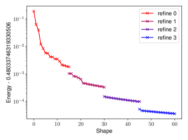
Figure 1: On the left is the energy and on the right discrete Hausdorff complementary distance along the shape iterates for the experiment in Section 5.2.1. We see that the energy is reducing along the shapes, jumping to a lower energy when the mesh is refined and the distance decreases on average.

For convergence of our scheme, in Theorem 4.4, we require that $\|D\Phi_{h}\|_{L^{\infty}}$ and $\|D\Phi_{h}^{-1}\|_{L^{\infty}}$ are bounded; the value of these along the iterations is found in Figure 2

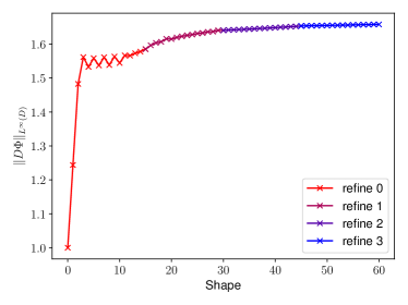
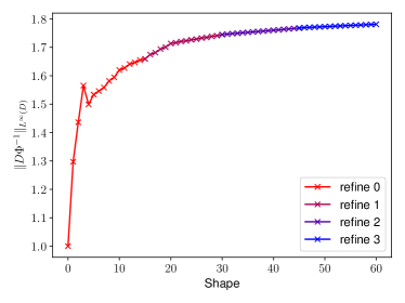
Figure 2: Values for $\|D\Phi_{h}\|_{L^{\infty}}$ (left) and $\|D\Phi_{h}^{-1}\|_{L^{\infty}}$ (right) along the shape iterates for the experiment in Section 5.2.1. We see that the values of $\|D\Phi_{h}\|_{L^{\infty}}$ and $\|D\Phi_{h}^{-1}\|_{L^{\infty}}$ abruptly jump up at the start, and only slowly increase later on.

The final domains are given on the right of Figure 3.

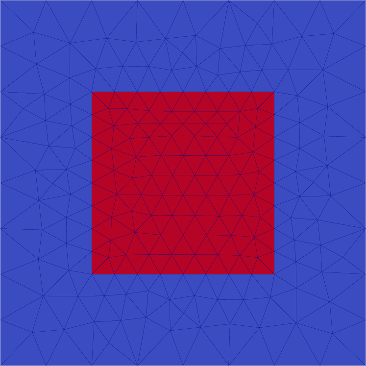
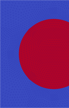
Figure 3: Final domains for the experiment in Section 5.2.1, refinements increasing from top left to bottom right. Taking the maximum over all triangles, the radius ratio for the initial grid is $\tilde{\sigma}_{0}\approx 1.633917$ and for the final, most fine, grid is $\tilde{\sigma}_{f}\approx 1.651944$.

5.2.2 Experiment 2

For this experiment, we consider $j(\cdot,u,z):=\frac{1}{2}(u-u_{d})^{2}$, where we choose

$$u_{d}(x)=5\frac{-\pi|x|^{2}\ln(4)+3\ln(|x|^{2})+3\ln(\pi)+\ln(4)}{\pi\ln(256)},$$

for the data for the Poisson problem, we take $f=5$. Notice that $u_{d}$ has zeros on $|x|=\frac{1}{\sqrt{\pi}},\,\frac{2}{\sqrt{\pi}}$ and that $-\Delta u_{d}=f$.

The optimal shape is expected to be $\Omega^{*}:=B(0,\frac{2}{\sqrt{\pi}})\setminus\overline{B(0,\frac{1}{\sqrt{\pi}})}$, with $\mathcal{J}(\Omega^{*})=0$. As in the first experiment, this is again calculated using axi-symmetric arguments. Notice that this is not a simply connected optimal shape, which may require some topology optimisation. We choose the initial domain given by an approximation of $\hat{\Omega}=B(0,1.4)\setminus\overline{B(0,0.7)}$. Let us note that, without prior knowledge of the topology of the domain, e.g. starting with a ball of radius $1$, the domains heads towards a non-axi-symmetric shape, which may possibly end up in a degenerate minimiser. A combined shape and topology optimisation may prove useful in such a setting. The development of this is work in preparation.

The initial mesh is displayed on the left of Figure 6, with the hold all in blue, and the initial domain in red.

In Figure 4, we see the energy and the discrete Hausdorff complementary distance (5.2) for the experiment along the iterations.

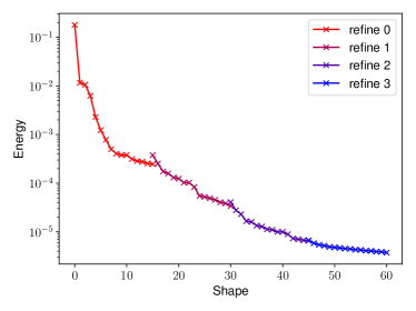
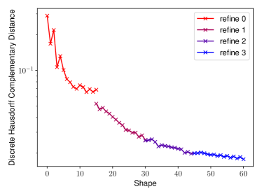
Figure 4: On the left is the energy and on the right discrete Hausdorff complementary distance along the shape iterates for the experiment in Section 5.2.2. We see that the energy is decreasing, jumping up as the mesh is refined. However, the energy recovers only a few steps later to a value smaller than the coarser mesh. The distance is reducing on average along the iterations, rarely increasing

The value of $\|D\Phi_{h}\|_{L^{\infty}}$ and $\|D\Phi_{h}^{-1}\|_{L^{\infty}}$ along the iterations is found in Figure 5.

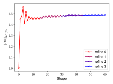
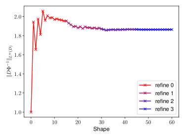
Figure 5: Values for $\|D\Phi_{h}\|_{L^{\infty}}$ (left) and $\|D\Phi_{h}^{-1}\|_{L^{\infty}}$ (right) along the shape iterates for the experiment in Section 5.2.2. We see again that the values of $\|D\Phi_{h}\|_{L^{\infty}}$ and $\|D\Phi_{h}^{-1}\|_{L^{\infty}}$ abruptly jump up at the start. Later on, $\|D\Phi_{h}^{-1}\|_{L^{\infty}}$ appears to plateau and $\|D\Phi_{h}\|_{L^{\infty}}$ increases only very slightly.

The final domains are given on the right of Figure 6.

Figure 6: On the left is the initial domain and on the right is a quarter of the final domains for the experiment in Section 5.2.2, refinements increasing from top left to bottom right. Taking the maximum over all triangles, the radius ratio for the initial grid is $\tilde{\sigma}_{0}\approx 1.787287$ and for the final, most fine, grid is $\tilde{\sigma}_{f}\approx 1.917235$.

5.2.3 Experiment 3

For this experiment, we choose $f=1$ and consider $j(x,u,z):=\frac{1}{2}|z+\frac{x}{2}|^{2}$ along with a penalty for the volume as in Remark 4.1, where we set $m_{0}=4$. Without the penalty term and for this choice of $j$, it holds that for any $r>0$, the balls $B_{r}(0)$ would be a minimiser with $0$ energy. By penalising the volume to be equal to $4$, one has that the minimiser will be the ball of radius $r=\frac{2}{\sqrt{\pi}}$, with $\mathcal{J}(\Omega^{*})=0$.

As remarked at the beginning of this section, this experiment is performed slightly differently to the previous two. While we will cascade to a finer mesh after a maximum of 15 steps, we will also continue with the shape optimisation to provide the first shape which is produced with an Armijo step of $2^{-11}$. This allows for a fair comparison of how the energy and Hausdorff complementary distance appear when the shape is approximately stationary. When we refine through the cascade, we will increase the penalty parameter so that it scales like $h^{-\frac{1}{2}}$.

For this experiment, we use a symmetric grid, rather than one generated by pygmsh. The initial domain, given by $\hat{\Omega}=(-1,1)^{2}$, appears in red on the left of Figure 9, with the hold all in blue.

In Figure 7, we see the energy and the discrete Hausdorff complementary distance (5.2) for the experiment along the iterations.

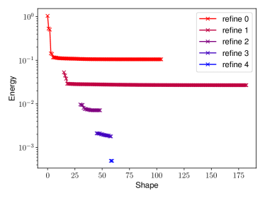
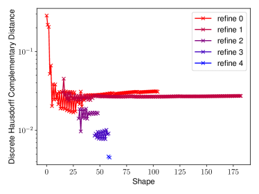
Figure 7: On the left is the energy and on the right discrete Hausdorff complementary distance along the shape iterates for the experiment in Section 5.2.3. We see that the energy is reducing along the shapes, jumping to a lower energy when the mesh is refined. The coarser grids require many more shape updates to reach the prescribed convergence criteria than the finer grids.

In Table 1, we tabulate the mesh size of the reference domain for each of the approximately converged shape along with the associated energy and discrete Hausdorff complementary distance. We also provide the experimental order of convergence, which for a given functional $E(h)$, here depending on the size $h$ of the reference mesh, is defined by

$$EOC:=\frac{\ln{E(h_{1})}-\ln{E(h_{2})}}{\ln{h_{1}}-\ln{h_{2}}}.$$

$h$	$\mu_{h}$	Energy	EOC Energy	HCD	EOC HCD
0.5	0.5	0.105327	–	0.0308699	–
0.25	$\frac{1}{\sqrt{2}}$	0.0268579	1.97146	0.0273133	0.176597
0.125	1	0.00712922	1.91353	0.016456	0.730993
0.0625	$\sqrt{2}$	0.00179752	1.98774	0.00912092	0.851362
0.03125	2	0.000493593	1.86461	0.00451768	1.0136

Table 1: Energy and discrete Hausdorff complementary distance for the final domains for each refinement level for the experiment in Section 5.2.3. We see a clear decrease in the Energy and the Discrete Hausdorff Complementary Distance as we refine the mesh.

The value of $\|D\Phi_{h}\|_{L^{\infty}}$ and $\|D\Phi_{h}^{-1}\|_{L^{\infty}}$ along the iterations is found in Figure 8

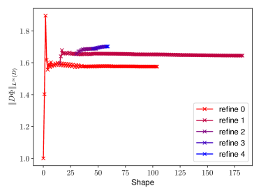
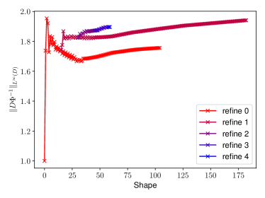
Figure 8: Values for $\|D\Phi_{h}\|_{L^{\infty}}$ (left) and $\|D\Phi_{h}^{-1}\|_{L^{\infty}}$ (right) along the shape iterates for the experiment in Section 5.2.3. As in the previous experiments, the values of $\|D\Phi_{h}\|_{L^{\infty}}$ and $\|D\Phi_{h}^{-1}\|_{L^{\infty}}$ abruptly jump up at the start. We see for the coarser grids that $\|D\Phi_{h}^{-1}\|_{L^{\infty}}$ increases a large amount relative to the finer grids. For the finer grids, both values appear very stable with minimal increase beyond the initial jump.

The final domains are given on the right of Figure 9.

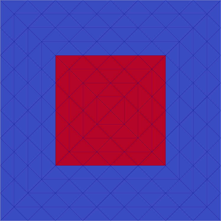
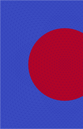
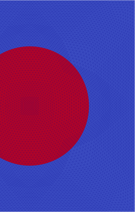
Figure 9: Final domains for the experiment in Section 5.2.3, refinements increasing from top left to bottom right. The most refined mesh is not shown due to the very small triangles. Taking the maximum over all triangles, the radius ratio for the initial grid is $\tilde{\sigma}_{0}=\frac{1}{2}+\frac{1}{\sqrt{2}}\approx 1.207107$ and for the final, most fine, grid is $\tilde{\sigma}_{f}\approx 1.489403$.

6 Conclusions

This work presents a numerical finite element solution framework for discrete PDE constrained shape optimisation in the $W^{1,\infty}$-topology based on the steepest descent method with Armijo step size rule. In Theorem 3.3, global convergence of this method is shown for a fixed discretisation parameter. Moreover, in Theorem 4.4 it is shown that a sequence of discrete stationary shapes under assumption (A2) converges with respect to the Hausdorff complementary metric to a stationary point of the limit problem (1.1) for the mesh parameter tending to zero. The proof of this result is based on the continuity of the Dirichlet problem with respect to the Hausdorff complementary metric in terms of $\gamma$–convergence.

In future work our numerical concept and convergence analysis could be extended to the numerical investigation of shape Newton methods in the $W^{1,\infty}$-topology, which we addressed in [DHH23], or that of transformations which preserve some geometric quantity, as in [HES23].

References

- [ADJ21] Grégoire Allaire, Charles Dapogny and François Jouve “Shape and topology optimization” In Differential Geometric Partial Differential Equations: Part II 22, Handbook of Numerical Analysis Amsterdam, Netherlands: Elsevier, 2021, pp. 3–124
- [BM20] S. Bartels and M. Milicevic “Efficient iterative solution of finite element discretized nonsmooth minimization problems” In Comput. Math. Appl. 80.5, 2020, pp. 588–603 DOI: 10.1016/j.camwa.2020.04.026
- [BW20] Sören Bartels and Gerd Wachsmuth “Numerical Approximation of Optimal Convex Shapes” In SIAM Journal on Scientific Computing 42.2, 2020, pp. A1226–A1244 DOI: 10.1137/19M1256853
- [Bas+21] Peter Bastian et al. “The Dune framework: Basic concepts and recent developments” Development and Application of Open-source Software for Problems with Numerical PDEs In Computers & Mathematics with Applications 81, 2021, pp. 75–112 DOI: https://doi.org/10.1016/j.camwa.2020.06.007
- [CZ06] D. Chenais and Enrique Zuazua “Finite-element approximation of 2D elliptic optimal design” In Journal de Mathématiques Pures et Appliquées 85.2, 2006, pp. 225–249 DOI: https://doi.org/10.1016/j.matpur.2005.05.001
- [DHH22] Klaus Deckelnick, Philip J. Herbert and Michael Hinze “A novel approach to shape optimisation with Lipschitz domains” In ESAIM: COCV 28, 2022, pp. 2 DOI: 10.1051/cocv/2021108
- [DHH23] Klaus Deckelnick, Philip J. Herbert and Michael Hinze “Shape optimisation in the topology with the ADMM algorithm” In arXiv preprint arXiv:2301.08690, 2023
- [DN18] Andreas Dedner and Martin Nolte “The Dune Python Module” In arXiv preprint 1807.05252, 2018 ARXIV ̵PREPRINT ̵ARXIV:1807.05252: 1807.05252
- [DNK20] Andreas Dedner, Martin Nolte and Robert Klöfkorn “Python Bindings for the DUNE-FEM module” Zenodoo, 2020 DOI: 10.5281/zenodo.3706994
- [DZ01] M.. Delfour and J.-P. Zolésio “Shapes and Geometries: Analysis, Differential Calculus, and Optimization” USA: Society for IndustrialApplied Mathematics, 2001
- [DZ11] M.C. Delfour and J.P. Zolesio “Shapes and Geometries: Metrics, Analysis, Differential Calculus, and Optimization, Second Edition”, Advances in Design and Control Society for IndustrialApplied Mathematics (SIAM, 3600 Market Street, Floor 6, Philadelphia, PA 19104), 2011 URL: https://books.google.co.uk/books?id=fjjvX9a9cxUC
- [EHS07] Karsten Eppler, Helmut Harbrecht and Reinhold Schneider “On convergence in elliptic shape optimization” In SIAM Journal on Control and Optimization 46.1 SIAM, 2007, pp. 61–83
- [FPV15] Ivan Fumagalli, Nicola Parolini and Marco Verani “Shape optimization for Stokes flows: a finite element convergence analysis” In ESAIM: Mathematical Modelling and Numerical Analysis 49.4 EDP Sciences, 2015, pp. 921–951
- [GZ21] Wei Gong and Shengfeng Zhu “On discrete shape gradients of boundary type for PDE-constrained shape optimization” In SIAM Journal on Numerical Analysis 59.3 SIAM, 2021, pp. 1510–1541
- [HKM18] Juha Heinonen, Tero Kipelainen and Olli Martio “Nonlinear potential theory of degenerate elliptic equations” Courier Dover Publications, 2018
- [HP18] Antoine Henrot and Michel Pierre “Shape Variation and Optimization: A Geometrical Analysis”, EMS tracts in mathematics European Mathematical Society, 2018 URL: https://books.google.co.uk/books?id=%5C_fCqswEACAAJ
- [HES23] Philip J. Herbert, Jose A. Escobar and Martin Siebenborn “Shape optimization in with geometric constraints: a study in distributed-memory systems” In arXiv preprint arXiv:2309.15607, 2023 arXiv:2309.15607 [math.OC]
- [Hin+08] Michael Hinze, René Pinnau, Michael Ulbrich and Stefan Ulbrich “Optimization with PDE constraints” Springer Science & Business Media, 2008
- [HPS15] Ralf Hiptmair, Alberto Paganini and Sahar Sargheini “Comparison of approximate shape gradients” In BIT Numerical Mathematics 55.2 Springer, 2015, pp. 459–485
- [ISW18] José A Iglesias, Kevin Sturm and Florian Wechsung “Two-dimensional shape optimization with nearly conformal transformations” In SIAM Journal on Scientific Computing 40.6 SIAM, 2018, pp. A3807–A3830
- [KV13] Bernhard Kiniger and Boris Vexler “A priori error estimates for finite element discretizations of a shape optimization problem” In ESAIM: Mathematical Modelling and Numerical Analysis-Modélisation Mathématique et Analyse Numérique 47.6, 2013, pp. 1733–1763
- [Sch22] Nico Schlömer “pygmsh: A Python frontend for Gmsh” If you use this software, please cite it as below. Zenodo, 2022 DOI: 10.5281/zenodo.5913837
- [SZ92] J. Sokołowski and J.P. Zolésio “Introduction to Shape Optimization: Shape Sensitivity Analysis”, Lecture Notes in Computer Science Springer-Verlag, 1992 URL: https://books.google.de/books?id=hg-oAAAAIAAJ
- [ZG19] Shengfeng Zhu and Zhiming Gao “Convergence analysis of mixed finite element approximations to shape gradients in the Stokes equation” In Computer Methods in Applied Mechanics and Engineering 343 Elsevier, 2019, pp. 127–150
- [ZHL20] Shengfeng Zhu, Xianliang Hu and Qifeng Liao “Convergence analysis of Galerkin finite element approximations to shape gradients in eigenvalue optimization” In BIT Numerical Mathematics 60 Springer, 2020, pp. 853–878