MGAS: Multi-Granularity Architecture Search for Trade-Off Between Model Effectiveness and Efficiency

Abstract

Neural architecture search (NAS) has gained significant traction in automating the design of neural networks. To reduce the time cost, differentiable architecture search (DAS) transforms the traditional paradigm of discrete candidate sampling and evaluation into that of differentiable super-net optimization and discretization. However, existing DAS methods fail to trade off between model performance and model size. They either only conduct coarse-grained operation-level search, which results in redundant model parameters, or restrictively explore fine-grained filter-level and weight-level units with pre-defined remaining ratios, suffering from excessive pruning problem. Additionally, these methods compromise search quality to save memory during the search process. To tackle these issues, we introduce multi-granularity architecture search (MGAS), a unified framework which aims to discover both effective and efficient neural networks by comprehensively yet memory-efficiently exploring the multi-granularity search space. Specifically, we improve the existing DAS methods in two aspects. First, we balance the model unit numbers at different granularity levels with adaptive pruning. We learn discretization functions specific to each granularity level to adaptively determine the unit remaining ratio according to the evolving architecture. Second, we reduce the memory consumption without degrading the search quality using multi-stage search. We break down the super-net optimization and discretization into multiple sub-net stages, and perform progressive re-evaluation to allow for re-pruning and regrowing of previous units during subsequent stages, compensating for potential bias. Extensive experiments on CIFAR-10, CIFAR-100 and ImageNet demonstrate that MGAS outperforms other state-of-the-art methods in achieving a better trade-off between model performance and model size.

I Introduction

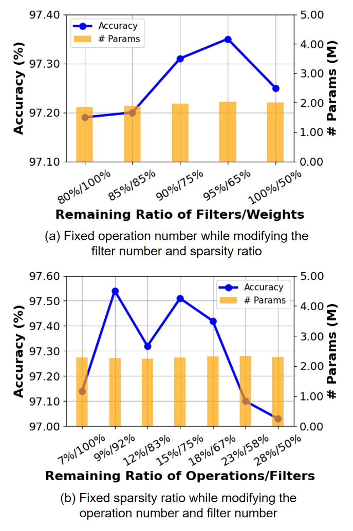
Figure 1: Illustration of the accuracy-parameter trade-off with respect to different remaining ratios for units at different granularity levels (operation, weight and filters) on CIFAR-10 dataset. In (a), we maintain a constant operation number and manipulate the filter number and sparsity ratio, while ensuring the model parameters remain unchanged at approximately 2M. In (b), we keep the sparsity ratio fixed and modify the operation number and filter number, while maintaining the model parameters at around 2.3M. We observe that model accuracy varies significantly even when model sizes are similar. This underscores the necessity of effectively balancing the units of different granularities.

Neural architecture search, the method for automatically designing effective and efficient neural networks, has gained significant popularity in various domains including computer vision [1, 2, 3] and natural language processing [1, 4]. In the early stage of NAS, architectures were heuristically sampled from a search space using reinforcement learning [5, 6] or evolutionary algorithms [7, 8], followed by individual training and performance comparison, which incurred significant computational cost. Weight-sharing techniques were later introduced to alleviate the burden by enabling the sharing of model weights among different architectures through a super-network created from the search space. By training only a single super-net, the computational resources required can be greatly reduced. Based on that, differentiable architecture search (DAS), e.g., DARTS [1], further improved the efficiency by introducing differentiable architecture parameters which can be optimized along with the super-net weights via gradient descent. This advancement allows for the direct updates of the architecture during super-net training, transforming the search process into the optimization and discretization of the super-net.

In spite of the great success of DAS, the current research mainly focuses on coarse-grained search in constrained search spaces that only cover operation-level searchable units. While this limited granularity stabilizes the search process, it inevitably results in the presence of redundant parameters in the discovered architectures, which consequently affects model efficiency.

To eliminate the redundancy, recent studies have emerged to expand the search space and investigate finer-grained units at the filter and weight levels. While certain studies [9, 10, 11] perform filter-level search, their methods are limited by determining the remaining filter ratio from a restricted set of options, which lacks flexibility. Moreover, they cannot be extended to weight-level search which offers a much broader range of sparsity pattern candidates. On the other hand, [12, 13] directly prune on weight-level units until the network reaches a manually-defined target sparsity ratio, aiming to discover well-performing highly-sparse architectures. However, it is worth noting that the sparsity ratio itself is a crucial factor influencing the model performance. It is also mentioned in [14] that there exists an optimal sparsity ratio for a specific neural network in terms of achieving the best performance. We further reveal that such performance discrepancies cannot be solely attributed to the differences in model sizes introduced by sparsity. Even models with similar parameter counts can exhibit significant performance variations depending on different remaining ratios of the operations, filters and weights, as shown in Fig. 1. This observation highlights the necessity of balancing the unit numbers at different granularity levels. Failure to consider the relative numbers of the multi-granularity units can lead to excessive pruning at certain levels, which degrades the model effectiveness.

Additionally, DAS requires the whole super-net to be placed in the memory for optimization and discretization, leading to substantial memory usage. This issue becomes more pronounced when the finer-grained searchable units are introduced. For example, in order to facilitate the flexible filter-level search, the initial super-net must possess a larger number of filters for candidate selection, which increases the demands of the memory. Several techniques have been proposed to save memory. The most commonly applied proxy strategy involves optimizing a shallower [1, 15, 16] or slimmer [17, 18] proxy super-net during the search, followed by extension of the discovered architecture to form the final target network. However, this configuration change renders the proxy strategy unsuitable for flexible fine-grained search. Another approach is the decomposition strategy, which factorizes the super-net along the path [19, 20, 21] or the depth [22, 23, 24] for separate optimization. Nevertheless, this strategy introduces bias and compromises the search quality, as the searchable units are prematurely evaluated without considering the overall architecture. As a result, there is a necessity to propose a more general and effective memory reduction strategy applicable to flexible and complex search spaces.

To address these issues, we propose multi-granularity architecture search (MGAS), which serves as a unified framework to comprehensively explore the multi-granularity search space in a memory-efficient way, aiming to discover neural networks that are both effective and efficient. Specifically, we balance the unit numbers of different granularities through an adaptive pruning scheme. This involves learning discretization functions specific to each granularity level during the search to adaptively adjust the pruning criteria for different granularities according to the evolving architecture. Consequently, the remaining ratios of units at different granularity levels can be properly determined for models at different target sizes. To reduce the memory consumption for this search space, we propose a multi-stage search strategy. This entails decomposing the super-net optimization and discretization into sequential sub-net stages. In each stage, the size of preceding sub-nets is significantly reduced, ensuring low memory usage. However, since the preceding sub-nets are greedily optimized without considering the structure of subsequent ones, the early stages are inevitably biased like existing decomposition methods. To compensate for the bias, we further propose to progressively re-evaluate the previous units as we move to the later stages, so that the remaining units in preceding sub-nets can undergo additional pruning, and the pruned units have the opportunity to regrow based on the subsequent sub-nets.

Through extensive experiments, our method demonstrates promising outcomes in various aspects. First, it reduces the model size without compromising the performance compared with coarse-grained methods. Second, it enhances the model performance while maintaining a similar model size compared with existing fine-grained methods. Third, it saves memory during the search process without diminishing the quality of the search.

The main contributions of this work can be summarized as follows:

1. To the best of our knowledge, we conduct the first in-depth study on balancing the unit numbers at different granularity levels in NAS to trade off between model effectiveness and model efficiency.

2. We propose an effective memory reduction strategy that can be applied to the expanded DARTS search spaces without compromising the search quality.

3. We demonstrate the superiority of MGAS through extensive experiments on CIFAR-10, CIFAR-100 and ImageNet. Compared with baseline methods, MGAS achieves a better trade-off between model performance and model size.

II Related works

In this section, we will first introduce the recent progress in the search space expansion in DAS. Then, we summarize widely employed memory reduction strategies.

II-A Search Space Expansion

For the search efficiency, prevalent DAS approaches often perform the search in cell-based search spaces [25], e.g., DARTS search space. Recent works relax the constraints within these search spaces to discover novel designs.

To enable flexible connection patterns, Amended-DARTS [26] explores independent cell structures. GOLD-NAS [27] allows each node to preserve an arbitrary number of precedents and each edge to preserve an arbitrary number of operations.

Other works turn to investigate finer-grained searchable units. Single-path NAS [9] jointly searches for the kernel size and expansion ratio by encoding all the candidate convolution operations into one single ’superkernel’. Trilevel NAS [11] also defines a set of searchable expansion ratios and performs the filter-level search with parameters indicating the probability of the choices. However, both works lack flexibility in determining the filter number as they are limited to several pre-defined options. Moreover, they cannot be extended to search for the various sparsity patterns that cannot be encoded into several options at the weight level. In comparison, SuperTickets [12] iteratively prunes unimportant filters and weights to identify efficient networks and their ’lottery subnetworks’. DASS [13] also directly utilizes pruning technique, and explores operation-level and weight-level units by incorporating two sparse candidate operations to find sparsity-friendly networks. Nevertheless, both works pre-define the desired sparsity ratio and ignore the exploration of the unit distribution at different granularity levels.

In this work, we follow the connection pattern settings in GOLD-NAS due to its high flexibility, and integrate operation-level, filter-level and weight-level units to form a multi-granularity search space, targeting at discovering a network that achieves a better accuracy-parameter trade-off. We specifically focus on identifying proper remaining ratios for units of different granularities.

II-B Memory Reduction Strategies

DARTS [1] and its subsequent works [15, 16, 13] apply a depth-level proxy strategy to save memory by searching for a network with repeatable cells in a shallower proxy super-net, and constructing a deeper target network with stacked cells. To fill the performance gap caused by the inconsistency between the proxy and target networks, PDARTS [28] progressively reduces the candidate operations and increases the network depth. PC-DARTS [17] applies the proxy strategy at the width level by sampling a sub-set of channels for optimization while bypassing the held out part in a shortcut. However, the extension of depth necessitates identical cell structures in the network and the extension of width requires identical sparsity patterns in the filters. Consequently, the proxy strategy is not applicable for conducting flexible fine-grained search in our multi-granularity search space.

In contrast, ProxylessNAS [19] proposes a path binarization strategy to activate only one or two paths in the super-net for optimization at each iteration. GDAS [20] utilizes the Gumbel-Max trick for the discrete sampling of the single-path architecture. To reduce the instability brought by sampling, MSG-DAS [21] extends the Gumbel sampler to optimize multiple mutually exclusive single-path architectures at each iteration. However, these methods cannot discover well-performed multi-path architectures due to their biased optimization of operations without considering counterparts on the same edge. DNA [22] factorizes the super-net along the depth into blocks and employs a pre-trained teacher model for block-wise supervision to enable separate optimization. BossNAS [23] uses self-supervised learning as an alternative to the supervised distillation. Sharing a similar decomposition idea, PNAS [24] starts with a small number of blocks, progressively removing the unpromising structures in previous blocks and extending the block number. However, the importance of previously evaluated units may vary in the complete architecture, which also introduces bias in the search process.

In this work, we aim to propose a general memory reduction strategy applicable to the multi-granularity search space yet effective enough to ensure high search quality.

III Preliminaries

In this section, we present the frequently studied single-granularity DARTS search space, aiming to establish a foundational understanding in preparation for the introduction of the multi-granularity search space in the next section.

III-1 DARTS Search Space

The original DARTS search space consists of multiple cells, wherein each cell is a directed acyclic graph encompassing an ordered sequence of $M$ computational nodes. Each node $x_{i}$ serves as a latent representation and each directed edge $(i,j)$ denotes the information transformation from $x_{i}$ to $x_{j}$. The operations $o$ on each edge need to be determined, where the operation types include convolutions with different kernel sizes, pooling and skip connection.

During the search, DARTS relaxes the discrete search space to be continuous by constructing a super-net incorporating all the operations and combining them utilizing differentiable architecture parameters. Within the super-net, the output of each node is the weighted sum of all its precedents. Mathematically, there is $x_{j}=\sum_{i<j}\sum_{o\in O}\sigma(\alpha_{i,j}^{o})\cdot o(x_{i})$, where $O$ indicates the candidate operation set, $o$ represents a candidate operation, $\alpha_{i,j}^{o}$ denotes the architecture parameter of the operation $o$ on the edge $(i,j)$, and $\sigma(\alpha_{i,j}^{o})$ signifies the scaled architecture parameter. In this way, the problem of selecting the operations $o$ is transformed into that of optimizing and discretizing the scaled architecture parameters $\sigma(\alpha)$.

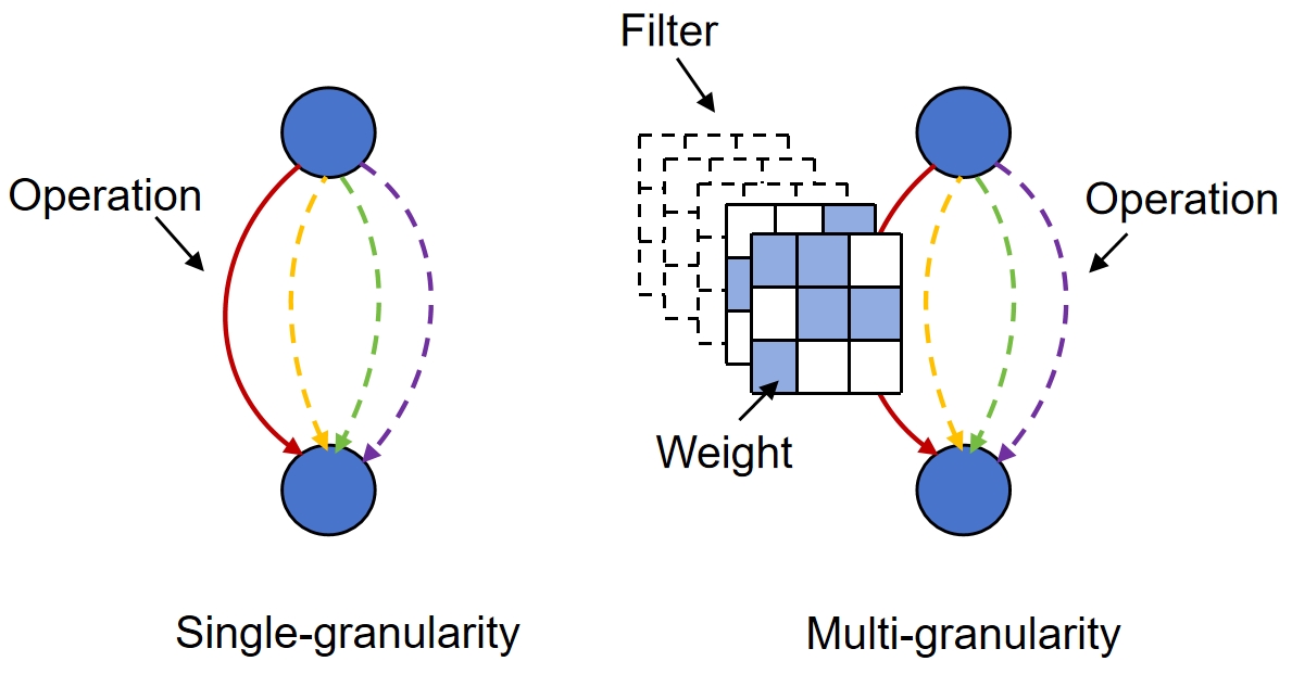
Figure 2: Illustration of the single-granularity and multi-granularity search space. The multi-granularity search space allows for the exploration of fine-grained filter-level and weight-level units, which enables a greater reduction of potential redundant parameters and facilitates the discovery of more light-weight yet effective models.

IV Methodology

In this section, we first describe the multi-granularity search space to be explored. Then, we introduce our proposed MGAS framework, which consists of 1) adaptive pruning to balance the remaining ratios of units at different granularity levels in the discovered networks, and 2) multi-stage search to reduce the memory usage without compromising the search quality.

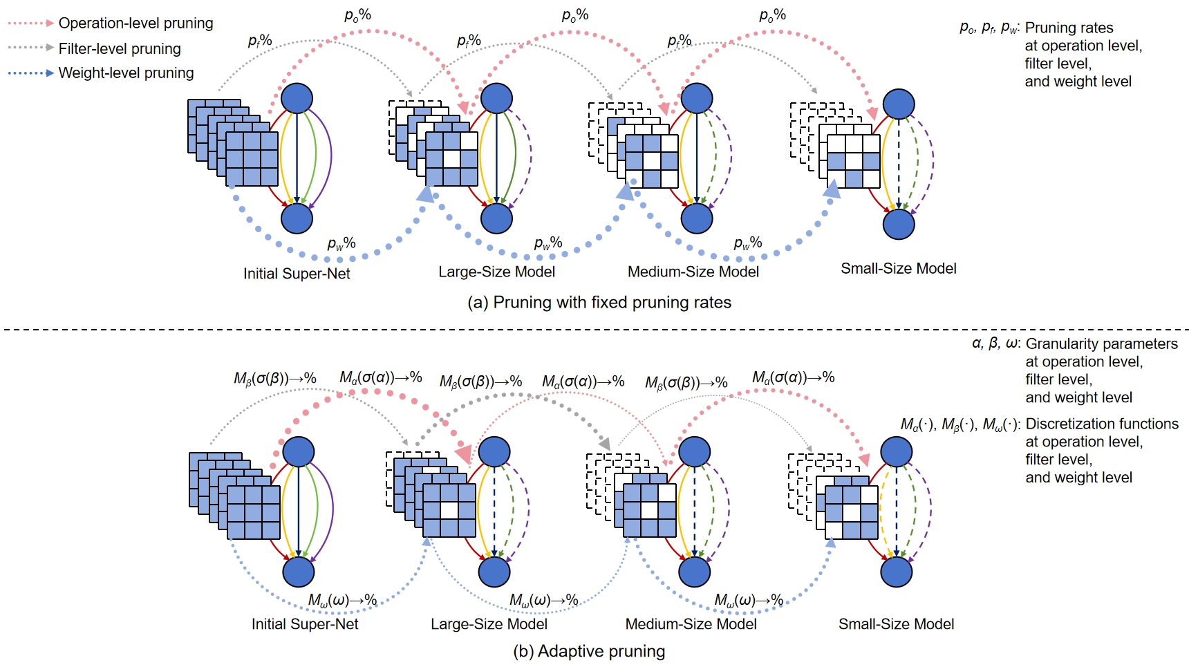
Figure 3: Overview of pruning with fixed pruning rates and adaptive pruning. The dotted arrows with different colours represent the pruning process at different granularity levels. The width of the dotted arrow indicates the number of the pruned units. Existing works independently prune on different granularities with fixed pruning rates. In contrast, our adaptive pruning learn granularity-specific discretization functions to adaptively determine the pruning number at each granularity level according to the architecture evolution, so that the relative remaining numbers at different levels can be optimized for models with different sizes.

IV-A Multi-Granularity Search Space

Compared with the single-granularity search space mentioned in the previous section, the multi-granularity search space covers not only operation-level but also filter-level and weight-level searchable units, as illustrated in Fig. 2. Specifically, apart from the operation type, we also need to determine the filter number and sparsity pattern in convolution operations.

The problem of searching for the proper filter number and sparsity pattern can be viewed as that of selecting the important subset of filters and weights from the super-net. The differentiable architecture parameter $\alpha$ can be viewed as the operation-level granularity parameter that represent the operation importance. Inspired by this, we introduce differentiable filter-level granularity parameter denoted as $\beta$ to indicate the significance of each filter. For an individual weight, we directly use the value of the weight itself $\omega$ to represent its importance. Mathematically, in each convolution operation $o(x_{i})$ in the constructed super-net, there is $C_{out}^{f}=\sigma(\beta^{f})\cdot\omega^{f}\cdot C_{in}$, where $C_{in}$ is the input feature map, $f$ refers to a filter, $C_{out}^{f}$ is the feature map generated by $f$, $\omega^{f}$ denotes the weights in the filter, $\beta^{f}$ represents the granularity parameter of $f$, and $\sigma(\beta^{f})$ is the scaled granularity parameter. In this super-net, we need to optimize and discretize the scaled granularity parameters of the three levels, i.e., $\sigma(\alpha)$, $\sigma(\beta)$ and $\omega$.

IV-B Adaptive Pruning

As discussed above, the primary concern in exploring the multi-granularity search space is the joint optimization and discretization of the scaled granularity parameters $\sigma(\alpha)$, $\sigma(\beta)$ and $\omega$. Previous studies [12, 13] have concentrated on improving joint optimization to accurately compare the unit importance within each granularity level. They achieve this by adaptively updating the granularity parameters of different levels, taking into account the changes in unit importance caused by the evolution of units at other levels. However, they independently discretize the granularity parameters at different levels with fixed pruning rates, failing to optimize the relative numbers of the remaining multi-level units. In this case, we focus on improving joint discretization with adaptive pruning to adaptively determine the relative numbers according to the evolving architecture. To achieve this, we need to enable the comparison of unit importance across different granularities. Given that the granularity parameters are measured on different scales, a direct numerical comparison is not feasible. Therefore, we propose the dynamic acquisition of granularity-specific pruning criteria to determine when a unit can be considered unimportant within its own granularity level along with the architecture evolution, enabling implicit comparison of unit importance across granularities.

Technically, instead of manually defining pruning rates or importance thresholds for discretization, we learn granularity-specific discretization functions $M_{\alpha}(\cdot),M_{\beta}(\cdot),M_{\omega}(\cdot)$ during the super-net optimization, as shown in Fig. 3. The objective of the discretization functions is to zero out the scaled granularity parameters $\sigma(\alpha),\sigma(\beta),\omega$ whose magnitudes are small enough. We formulate them as

$$M_{\alpha}(\sigma(\alpha))=S(|\sigma(\alpha)|-t_{\alpha})\cdot\sigma(\alpha),$$ (1)

$$M_{\beta}(\sigma(\beta))=S(|\sigma(\beta)|-t_{\beta})\cdot\sigma(\beta),$$ (2)

$$M_{\omega}(\omega)=S(|\omega|-t_{\omega})\cdot\omega,$$ (3)

where $S(\cdot)$ is a binary step function, $t_{\alpha},t_{\beta},t\omega$ are trainable thresholds. To make $S(\cdot)$ differentiable, we follow [29] to adopt a long-tailed higher-order estimator.

Considering the operation differences, we further refine $M_{\alpha}(\cdot),M_{\beta}(\cdot),M_{\omega}(\cdot)$ at the operation level to $M_{\alpha}^{o}(\cdot),M_{\beta}^{o}(\cdot),M_{\omega}^{o}(\cdot)$ in practice. Note that we have $M_{\alpha}^{o}(\cdot)$ for all kinds of operations, but only have $M_{\beta}^{o}(\cdot)$ and $M_{\omega}^{o}(\cdot)$ for convolution operations. Applied in the forward propagation of the super-net, there is

$$x_{j}=\sum_{i<j}\sum_{o\in O}M_{\alpha}^{o}(\sigma(\alpha_{i,j}^{o}))\cdot o(x_{i}),$$ (4)

and in each convolution operation $o$, there is

$$C_{out}^{f}=M_{\beta}^{o}(\sigma(\beta^{f}))\cdot M_{\omega}^{o}(\omega^{f})\cdot C_{in}.$$ (5)

By learning the discretization functions $M_{\alpha}(\cdot),M_{\beta}(\cdot),M_{\omega}(\cdot)$, we obtain tailored pruning criteria for each granularity adaptively according to the evolving architecture, so that the unit remaining ratios can be properly determined.

For a more stable search process, we follow the gradual pruning process proposed in [27]. This procedure involves conducting the discretization gradually along with the super-net optimization with regularization of resource efficiency (e.g., FLOPs), rather than all at once at the end. We prune out the units whose updated scaled granularity parameters $\sigma(\alpha),\sigma(\beta)$ or $\omega$ computed by $M_{\alpha}(\cdot),M_{\beta}(\cdot)$ or $M_{\omega}(\cdot)$ become zero after $e$ epochs. The overall adaptive pruning scheme is summarized in Algorithm 1.

At the operation level, the pruned operations are replaced with a non-parametric zero operation, which turns the input into zero. Considering the presence of skip connection operations, we align the number of filters in the output layer of each convolution operation within the same cell to match the average number of output filters among all convolution operations in the cell.

Algorithm 1 Adaptive Pruning

Input: dataset $D$, pruning interval $e$, target model size $Param_{min}$, initial remaining units $U_{act}$
Parameter: granularity parameters $\alpha,\beta,\omega$, thresholds $t_{\alpha},t_{\beta},t_{\omega}$
Output: an architecture consisting of the remaining units $U_{act}$

1:$epoch\leftarrow 0$

2:while $Param(U_{act})\geq Param_{min}$ do

3:     $epoch\leftarrow epoch+1$

4:     Update loss $L\leftarrow Loss(D;\alpha^{U_{act}},\beta^{U_{act}},\omega^{U_{act}})$ $\triangleright$ Optimization

5:     Update $\alpha^{U_{act}},\beta^{U_{act}},\omega^{U_{act}}$ by gradient descent based on $L$

6:     Update $t_{\alpha},t_{\beta},t_{\omega}$ by gradient descent based on $L$

7:     for each operation $o$ in $U_{act}$ do $\triangleright$ Discretization

8:         Update $\sigma(\alpha^{o})$ with discretization function $M_{\alpha}^{o}(\cdot)$: $\sigma(\alpha^{o})\leftarrow S(|\sigma(\alpha^{o})|-t_{\alpha}^{o})\cdot\sigma(\alpha^{o})$

9:         if $epoch\bmod e=0$ then

10:              if $\sigma(\alpha^{o})=0$ then

11:                  Update remaining units $U_{act}\leftarrow U_{act}\setminus o$

12:                  continue

13:              end if

14:         end if

15:         for each filter $f$ in $o$ do

16:              Update $\sigma(\beta^{f})$ with discretization function $M_{\beta}^{o}(\cdot)$: $\sigma(\beta^{f})\leftarrow S(|\sigma(\beta^{f})|-t_{\beta}^{o})\cdot\sigma(\beta^{f})$

17:              if $epoch\bmod e=0$ then

18:                  if $\sigma(\beta^{f})=0$ then

19:                       Update remaining units $U_{act}\leftarrow U_{act}\setminus f$

20:                       continue

21:                  end if

22:              end if

23:              for each weight $w$ in $f$ do

24:                  Update $\omega^{w}$ with discretization function $M_{\omega}^{o}(\cdot)$: $\omega^{w}\leftarrow S(|\omega^{w}|-t_{\omega}^{o})\cdot\omega^{w}$

25:                  if $epoch\bmod e=0$ then

26:                       if $\omega^{w}=0$ then

27:                           Update remaining units $U_{act}\leftarrow U_{act}\setminus w$

28:                           continue

29:                       end if

30:                  end if

31:              end for

32:         end for

33:     end for

34:end while

IV-C Multi-Stage Search

The high memory consumption of DAS comes from the large number of parameters in the super-net and their corresponding gradients. We maintain low memory consumption by breaking down the super-net optimization and discretization into multiple sub-net stages. Different from previous decomposition-based methods, we enable re-evaluation of the remaining and pruned units to compensate for the potential degradation of search quality caused by bias, as illustrated in Fig. 4.

Let the the search space of the whole architecture be N. To realize the multi-stage search, we decompose $N$ into sequential n moderate-size search spaces $N_{1},...,N_{i},...,N_{n}$ along the network depth, where $N_{i+1}$ is originally connected with $N_{i}$. In this way, the super-net constructed from the search space is naturally separated into n sub-nets with much smaller sizes. We first coarsely search for the sub-net structures in various stages, removing most of the unimportant units, and then fine-tune the remaining architecture until the target model size is achieved.

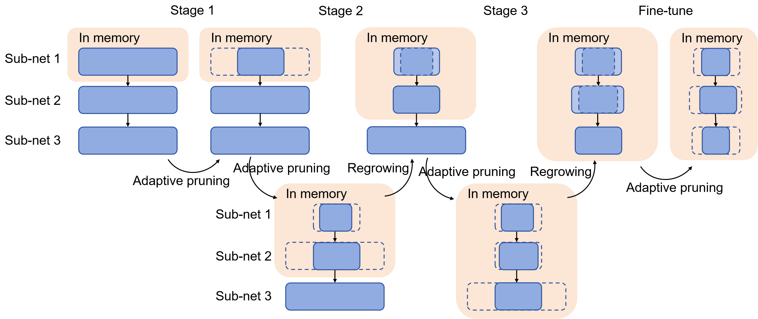
Figure 4: Illustration of multi-stage search. We decompose the super-net optimization and discretization into multiple sub-net stages to save memory, and enable further pruning and regrowing of the units in previous sub-nets during subsequent stages to reduce bias.

Algorithm 2 Multi-Stage Search

Input: dataset $D$, target model size $Param_{min}$, sub-net number $n$, target sub-net size $Param_{min}^{s}$ ($s=0,1,...,n$), pruning interval $e$, regrowing ratio $r$, units in the search space $U$
Parameter: scaled granularity parameters ${\sigma(\alpha),\sigma(\beta)}$, ${\omega}$, pruned operation number $num_{p}$, remaining units $U_{act}$
Output: an architecture consisting of the remaining units $U_{act}$

1:Initialize remaining units $U\leftarrow\emptyset$

2:for stage $s=0,1,...,n$ do

3:     Initialize pruned operation number $num_{p}\leftarrow 0$

4:     Update remaining units $U_{act}\leftarrow U_{act}\cup{U^{sub-net_{s}}}$

5:     while $Param(U_{act})\geq Param_{min}^{s}$ do $\triangleright$ Pruning

6:         Adaptive Pruning on $U_{act}$

7:         Update pruned operation number $num_{p}\leftarrow num_{p}+num^{prune}$

8:     end while

9:     for each cell $c$ in $U^{act}$ do $\triangleright$ Regrowing

10:         for each operation type $T$ in $c$ do

11:              Calculate regrowing potential $p^{T}_{c}$

12:              Calculate regrowing number ${num_{r}}^{T}_{c}\leftarrow num_{p}\times r\times p^{T}_{c}$

13:              Regrow ${num_{r}}^{T}_{c}$ operations of type $T$ in cell $c$

14:              Update remaining units $U_{act}\leftarrow U_{act}\cup U^{regrow}$

15:         end for

16:     end for

17:end for

18:while $Param(U_{act})\geq Param_{min}$ do $\triangleright$ Fine-tune

19:     Adaptive Pruning on $U_{act}$

20:end while

To supervise the optimization of the sub-net, we add task-specific output layers with predefined structure on top of each sub-net to generate results, so that the ground truth can be directly used as the supervision signal. However, since the task-specific output layers differ from the actual high-level layers in the target network, there is bias when optimizing previous sub-nets. To be specific, due to the complex interconnections between different units, the importance of the same unit in previous sub-nets may greatly change with the evolution of the following sub-nets.

To mitigate the bias, we perform progressive re-evaluation of units in preceeding sub-nets. On one hand, we continue to update the discretization functions for preceeding sub-nets during subsequent stages to further prune unimportant units. In practice, we set different pruning intervals, denoted as $e1$ and $e2$, for units in preceding sub-nets and the current sub-net. Notably, $e1$ is set to be larger than $e2$ to primarily focus on pruning in the current sub-net, while allowing longer optimization process before discretization for the previous sub-nets that have already undergone substantial pruning.

On the other hand, we estimate the potential of the pruned units for regrowing. Since the regrowth of operations will reinstate filters and weights, we mainly focus on the operation-level regrowing. Intuitively, if certain operations in a cell have a substantial impact on network performance at a given moment, reinserting the same operations in that cell should prove beneficial. Thus, we assess the regrowing potential for each operation type individually across different cells.

Inspired by [29], we utilize both the mean magnitude and the mean momentum of the granularity parameters $\alpha$ of each operation type in each cell to indicate the potential. The magnitude measures the direct contribution of the operation to accuracy, while the momentum gauges the persistent error reduction ability of the operation through the exponentially smoothed gradients. The momentum is formulated as

$$mom(\sigma(\alpha))^{t}=\beta\cdot mom(\sigma(\alpha))^{t-1}+(1-\beta)\cdot\frac{\partial L}{\partial\sigma(\alpha)}^{t-1},$$ (6)

where $\beta$ is a smoothing factor and $L$ is the loss. Therefore, the potential of the operation type $T$ in cell $c$, $p_{c}^{T}$, can be calculated as following:

$$mean\_mag_{c}^{T}=\frac{\sum_{j<M}\sum_{i<j}\sigma(\alpha_{c_{i,j}}^{T})}{\sum_{j<M}\sum_{i<j}S(\sigma(\alpha_{c_{i,j}}^{T}))},$$ (7)

$$mean\_mom_{c}^{T}=\frac{\sum_{j<M}\sum_{i<j}mom(\sigma(\alpha_{c_{i,j}}^{T}))}{\sum_{j<M}\sum_{i<j}S(\sigma(\alpha_{c_{i,j}}^{T}))},$$ (8)

$$p_{c}^{T}=\frac{1}{2}(mean\_mag_{c}^{T}+mean\_mom_{c}^{T}).$$ (9)

We set one hyper-parameter, the regrowing ratio $r$, to control the regrowth number $num_{r}$:

$$num_{r}=r\cdot num_{p},$$ (10)

where $num_{p}$ is the number of pruned operations.

Based on the calculated regrowing potential, we allocate the regrowing quota to different operation types in different cells. Within each operation type in a cell, we provide an equal chance for each pruned operation to be recovered through random sampling. When an operation is recovered, it replaces the zero operation in the super-net. To prevent a significant drop in performance caused by the insertion of useless operations, we initialize the recovered operations using the granularity parameters from before pruning, which are small enough. Consequently, only genuinely important operations will prevail in subsequent stages. The overall algorithm can be seen in Algorithm 2.

V Experiments

In this section, we evaluate MGAS on CIFAR-10, CIFAR-100 and ImageNet with various baseline methods. We try to answer the following research questions:

1. RQ1: Can MGAS discover an architecture with a better accuracy-efficiency trade-off compared with baselines?

2. RQ2: Can adaptive pruning consistently achieve a better balance in unit numbers of different granularities for models at different target sizes?

3. RQ3: Can multi-stage search save memory without compromising the search quality?

Different variants for each proposed component in MGAS is also discussed within the sub-sections.

V-A Datasets

We evaluate our method on CIFAR-10, CIFAR-100 and ImageNet-1k, which are image classification datasets:

1. CIFAR-10: 10 classes of images with the resolution of $32\times 32$. It has 50K training images and 10K test images.

2. CIFAR-100: 100 classes of images with the resolution of $32\times 32$. It has 50K training images and 10K test images.

3. ImageNet-1k: 1000 classes of images with the resolution of $224\times 224$. It has 1.3M training images and 50K validation images.

Following the widely adopted ImageNet dataset setting [17, 30], we use only 10% training data during the search to reduce time.

V-B Implementation Details

Search Space

We follow the configurations of common DARTS-series search spaces [1, 17, 28]. There are two kinds of cells: Normal cells which maintain the resolution and channel number; Reduction cells which reduce the resolution by half and double the channel number. The reduction cells are set at the 1/3 and 2/3 of the depth of the architecture. The candidate operation set consists of 7 operations. And we remove most of the manual constraints on the search space as in [27]: Each edge can preserve an arbitrary number of operations, each node can preserve an arbitrary number of predecessors, and all the cells can have different structures. Moreover, we search for not only the operation types, but also the filter numbers and sparsity patterns in convolution operations.

Hyper-parameters Settings

During the search, we decompose the super-net into three sub-nets according to the feature map resolution, i.e., $n$ is 3, where the later two sub-nets start with the two reduction cells. In each sub-net stage, we prune the network until its parameter number is reduced by half. The pruning intervals for preceding and current sub-nets, $e1$ and $e2$, are set 6 and 2 respectively. The regrowing ratio $r$ is set 0.2. In the fine-tuning process, we prune the network until reaching the target model size. We also apply the Cutout [31] and AutoAugment [32] techniques, as well as the warm-up technique to train the model weights for 5 epochs before the joint optimization with granularity parameters [17, 28]. The search process is conducted with a single NVIDIA A40 GPU. It takes around 2 days to search on CIFAR-10.

V-C Baselines

For fair comparison, we choose baseline methods that are also performed in DARTS-series search spaces.

Most of existing methods fall under the category of coarse-grained methods. Hence, we select eight representative coarse-grained methods with different memory reduction strategies from the past five years: (1) DARTS [1], (2) P-DARTS [28], (3) PC-DARTS [17], (4) GDAS [20], (5) GOLD-NAS [27], (6) MSG-DAS [21], (7) CDARTS [15], (8) MR-DARTS [16], along with one latest fine-grained method: (9) DASS [13] as baselines for CIFAR-10 and CIFAR-100 dataset, as shown in Table I. Among these methods, (1)-(3), (7)-(8) and (9) employ a proxy strategy to save memory, while (4) and (6) apply a decomposition strategy, and (5) directly reduces the candidate operation types.

We further select the baselines which report their model accuracy and model size on ImageNet for comparison on ImageNet dataset, as presented in Table II.

TABLE I: Comparison with SOTA methods on CIFAR-10 and CIFAR-100.

Method	Top-1 Accuracy (%)		# Params (M)	Top-1 Accuracy Density (%/M-params)		Granularity
	CIFAR-10	CIFAR-100		CIFAR-10	CIFAR-100
DARTSV1 [1]	97±0.14	82.24	3.3	29.39	24.92	operation
DARTSV2 [1]	97.24±0.09	82.46	3.3	29.47	24.99	operation
P-DARTS [28]	97.5	83.45	3.4	28.68	24.54	operation
PC-DARTS [17]	97.43±0.07	-	3.6	27.06	-	operation
GDAS [20]	97.07	81.62	3.4	28.55	24.01	operation
GOLD-NAS [27]	97.47	-	3.67	26.56	-	operation
MSG-DAS [21]	97.43	-	3.58±0.09	27.22	-	operation
CDARTS [15]	97.52 ± 0.04	84.31	3.9±0.08	25.01	21.62	operation
MR-DARTS [16]	97.51	83.56	4.3	22.68	19.43	operation
MGAS (ours, large)	97.34	83.58	2.1	46.37	39.8	operation, filter, weight
DASS [13] (small)	92.30	67.83	0.7	131.86	96.9	operation, weight
MGAS (ours, small)	96.51	80.61	0.68	141.93	118.54	operation, filter, weight

TABLE II: Comparison with SOTA methods on ImageNet. † indicates directly searching on ImageNet.

Method	Accuracy (%)		# Params (M)	Top-1 Accuracy Density (%/M-params)	Granularity
	Top-1	Top-5
DARTSV2 [1]	73.3	91.3	4.7	15.6	operation
P-DARTS [28]	75.6	92.6	4.9	15.43	operation
PC-DARTS [17]†	75.8	92.7	5.3	14.3	operation
GDAS [20]	74	91.5	5.3	13.96	operation
GOLD-NAS [27]†	76.1	92.7	6.4	11.89	operation
MSG-DAS [21]	75.2	92	5.4	13.93	operation
CDARTS [15]†	75.9	92.6	5.4	14.06	operation
MGAS†(ours, large)	75.5	92.6	4.6	16.41	operation, filter, weight
DASS [13] (small)	48.03	72.72	0.7	68.61	operation, weight
MGAS (ours, small)	65.48	86	0.68	96.29	operation, filter, weight

TABLE III: Memory consumption of MGAS in single-stage and multi-stage settings.

Method		Maximum Memory Consumption (G)
Single-stage search		30.7
	Stage 1	15.1
Multi-stage search	Stage 2	16.1
	Stage 3	16.5
	Fine-tune	13.3

TABLE IV: Comparison of MGAS with different regrowing ratios.

Regrowing Ratio $r$	Top-1 Accuracy (%)	# Params (M)	Top-1 Accuracy Density (%/M-params)
0	97.20	2.2	44.18
0.1	97.26	2.2	44.21
0.2	97.34	2.1	46.37

TABLE V: Comparison with SOTA methods in different search spaces on CIFAR10.

Method	Search Space 1		Search Space 2		Search Space 3		Memory Reduction Strategy
	Top-1 Accuracy (%)	# Params (M)	Top-1 Accuracy (%)	# Params (M)	Top-1 Accuracy (%)	# Params (M)
DARTSV1 [1]	96.85	1.23	96.69	1.37	-	-	Depth-level Proxy
PC-DARTS [17]	97.06	1.68	96.66	1.47	96.56	1.47	Width-level Proxy
GDAS [20]	96.78	0.95	95.34	0.65	96.11	1.13	Decomposition
MGAS	97.04	1.34	97.02	1.25	97.10	1.19	Multi-stage Search

V-D MGAS Discovers Architectures with a Better Accuracy-Efficiency Trade-Off (RQ1)

In this section, we verify whether MGAS can discover architectures with a better accuracy-efficiency trade-off compared with baselines.

V-D1 Results on CIFAR-10 and CIFAR-100

We impletement MGAS with two different search space settings. In order to compare with coarse-grained methods that prioritize accuracy, we start with a search space that contains relatively large models consisting of 14 cells and an initial filter number of 44. On the other hand, to compare with fine-grained methods that prioritize model efficiency and require higher search cost, we explore smaller models with 8 cells and an initial filter number of 24. For fair comparison, we use the same depth and initial width setting for the baseline DASS. We retrain the discovered architecture for 600 epochs for evaluation, and the results are shown in Table I. We utilize top-1 accuracy density [33] to measure the accuracy-efficiency trade-off, which quantifies how efficiently each model uses its parameters by dividing top-1 accuracy by parameter number.

Compared with coarse-grained methods, MGAS achieves comparable accuracy of around 97.4% and 83.5% on CIFAR-10 and CIFAR-100, respectively, using only 2.1M parameters. In the case of CIFAR-10, our method enables a reduction of up to 40% in model size compared to PC-DARTS and MSG-DAS while demonstrating a similar accuracy level with a marginal difference of 0.1%. For CIFAR-100, our method leads to a reduction of up to 45% in model size compared to P-DARTS and MR-DARTS at the same accuracy level. Additionally, MGAS outperforms all the baselines in terms of the top-1 accuracy density, showcasing the advantages of exploring a multi-granularity search space.

In comparison with fine-grained methods, MGAS converges to an architecture with a similar parameter count of approximately 0.7M, yet exhibits substantially higher accuracy. This demonstrates the benefits of balancing the remaining ratios of units at different granularity levels.

It is worth mentioning that the original DASS paper reports a promising result of 95.31% accuracy with only 0.1M parameters on CIFAR-10. However, their search space configuration, which contains models with 20 cells and an initial filter number of 36, differs from ours. As a result, the relative numbers of the remaining operations, filters and weights between their reported result and our implementation are different using the same discretization rules. This discrepancy has a surprisingly significant impact on model performance, underscoring the potential influence of relative unit numbers at different granularity levels. It indicates that methods relying on manually defined remaining ratios cannot guarantee performance without prior knowledge of the search space design, which further emphasizes the necessity of our method.

V-D2 Results on ImageNet

Similarly, we employ two different settings for ImageNet. To compare with coarse-grained methods, we explore large-size models with 14 cells and an initial filter number of 48. To compare with fine-grained methods, given their high search cost, we directly evaluate the small-size models discovered on CIFAR-10 using both MGAS and the baseline DASS instead of searching from scratch on Imagenet. In this way, we can also assess the generalization ability of the discovered architecture. We retrain the architectures for 250 epochs for evaluation, and the results are provided in Table II.

As shown in the table, MGAS surpasses all the baselines in terms of top-1 accuracy density, which indicates that MGAS can be generalized well to large datasets. Moreover, the transfered architecture discovered by MGAS demonstrates remarkably higher accuracy compared to that discovered by DASS. This highlights the strong generalization capability of the architectures generated by our method.

V-E Adaptive Pruning Consistently Achieves a Better Granularity Balance at Different Model Sizes (RQ2)

The superiority of MGAS over methods with manually defined ratios has already been demonstrated for certain model sizes. In this section, we verify whether adaptive pruning can consistently achieve a better granularity balance for different target model sizes.

To simplify the process, we only conduct operation-level and filter-level search. To eliminate the effect of multi-stage search, we employ the small search space setting with 8 cells and an initial filter number of 24, where the constructed super-net is small enough to be directly put into the memory without decomposition. Through one search process, we generate a series of architectures of varying sizes using adaptive pruning. Afterwards, we calculate the average pruning rates at both the operation and filter levels. The average pruning rates observed are 36 operations and 0.7% filters per two epochs. Based on this, we implement two basic gradual pruning methods with fixed pruning rates as baselines. Baseline 1 has higher operation-level pruning rates and lower filter-level pruning rates, while baseline 2 has higher filter-level pruning rates and lower operation-level pruning rates:

1. Fixed pruning rates 1: 44 operations and 0.3% filters per two epochs

2. Fixed pruning rates 2: 28 operations and 1.5% filters per two epochs

Employing these baseline methods, we obtain baseline architectures that exhibit variations in the remaining ratios at operation and filter levels. Here, the remaining ratio is defined as the ratio of the remaining unit number to the original unit number. For operations, the original unit number refers to the initial operation number in the super-net. For filters, the original unit number represents the initial filter number in operations within the discovered architecture.

The remaining ratios in the discovered architectures of adaptive pruning and the baselines are depicted in Fig. 5. As expected, baseline 1 generally retains more filters and fewer operations compared to adaptive pruning at similar model sizes. Conversely, baseline 2 preserves more operations and fewer filters. Moreover, it can be observed that adaptive pruning generates slimmer architectures at sizes of 1.05M and 1.17M, while producing wider architectures at smaller model sizes. This illustrates its ability to adaptively adjust the relative remaining ratios of operations and filters as the architecture evolves.

The performance of these methods is illustrated in Fig. 6. As displayed in the figure, adaptive pruning outperforms both baselines at all the model sizes, indicating its ability to consistently achieve a superior balance between granularities.

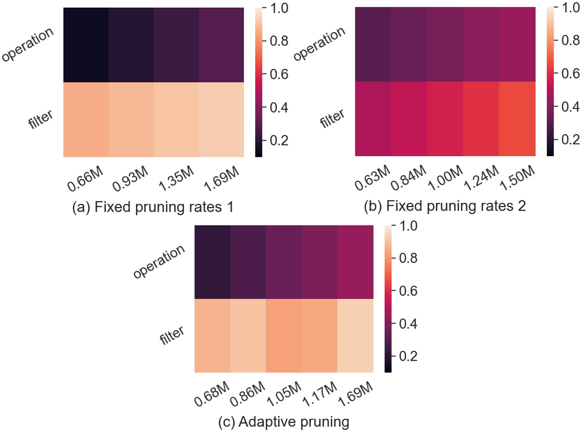
Figure 5: Remaining ratios of operations and filters in pruning with fixed pruning rates and our proposed adaptive pruning.

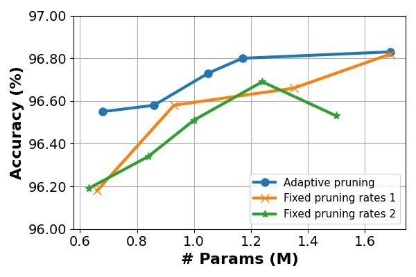
Figure 6: Performance of pruning with fixed pruning rates and our proposed adaptive pruning.

V-F Multi-Stage Search Ensures Low Memory Consumption with High Search Quality (RQ3)

In this section, we aim to assess the impact of multi-stage search on reducing memory consumption while maintaining high search quality.

V-F1 Reduction of memory consumption

To evaluate the reduction in memory consumption, we conduct a comparison between the search processes using both single-stage and multi-stage settings on CIFAR-10 in the small search space. The results are presented in Table III.

As shown in the table, the memory consumption reaches its peak at stage 3 in the multi-stage search, which is only 54% of the memory consumption observed in the single-stage search.

V-F2 Effect of hyper-parameter $r$

To assess the significance of the regrowing process and the effect of the hyper-parameter $r$, we conduct experiments comparing various regrowing ratios on CIFAR-10 in the large search space. The results are presented in Table IV.

From the table, it is apparent that the absence of the regrowing process, represented by $r$ equaling 0, leads to limited performance. This is reasonable since units that have been pre-maturely pruned cannot be recovered. As the value of $r$ increases, there is a corresponding improvement in accuracy from 97.20% to 97.34%. Such improvement can be attributed to the greater number of pruned units being re-evaluated in subsequent stages.

Note that the increase of $r$ will also add to the memory consumption and search cost. To avoid excessive burden on memory and time, we choose $r=0.2$ as the final setting and opt not to further increase its value.

V-F3 Preservation of search quality

To assess whether multi-stage search can consistently preserve high search quality, we compare it with other memory reduction strategies in different variations of the search space. To enable the comparison with proxy strategies, only operation-level search is conducted. To avoid any other confounding factors, adaptive pruning is not applied.

We choose DARTSV1, PC-DARTS and GDAS as baseline methods to represent depth-level proxy, channel-level proxy and decomposition strategies, respectively. We evaluate these methods on three 8-cell search spaces with an initial filter number of 36. Search space 1 represents the original DARTS search space. Search space 2 relaxes the connection constraint, allowing for the discovery of multi-path architectures. Search space 3 further relaxes the identical cell constraint, enabling different cell structures. The results are shown in Table V.

In search space 1, multi-stage search outperforms both DARTSV1 and GDAS in terms of accuracy and achieves similar performance with PC-DARTS, highlighting its effectiveness in preserving high search quality. After removing the manual constraints on the search spaces, the accuracy of the architectures discovered by both proxy and decomposition methods decrease significantly. Specifically, the path-level decomposition method GDAS performs poorly in Search Space 2, indicating its limited ability to explore multi-path architectures. Similarly, PC-DARTS, which performs well in search space 1, experiences a significant accuracy drop in search spaces 2 and 3, revealing the proxy strategy’s failure in preserving search quality when the search space exhibits more flexibility. In comparison, multi-stage search maintains high search quality in all the three search spaces.

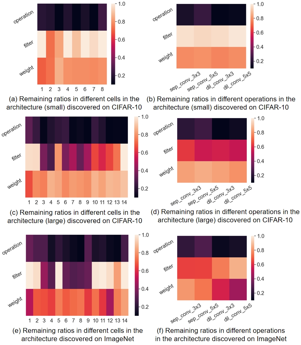
Figure 7: Distribution patterns of local units in discovered architectures. This figure illustrates the variance in unit distribution across different cells and operation types within the neural network architectures discovered on CIFAR-10 and ImageNet datasets. Notably, it highlights the preferences for fewer but wider and denser convolution operations in reduction cells, the predominance of $5\times 5$ separable convolution operation, and the variance in operation width and density between the middle and ends of large architectures. Differences in pattern preferences between the CIFAR-10 and ImageNet datasets are also depicted, reflecting the adaptation of the architecture to dataset complexity.

V-G Analysis of the Local Patterns in Discovered Architectures

In this section, we investigate the local unit distribution regarding the convolution operations inside the discovered architectures from Table I and II, aiming to provide insights for neural network design. The remaining ratios of units at different granularity levels regarding different cells and operations in the discovered architectures are demonstrated in Fig. 7.

Upon examination of the three architectures, it can be observed that reduction cells (cell 3 and 6 in the small architecture, cell 5 and 10 in the large architectures) tend to preserve wider and denser convolution operations, while the operation number is not necessarily large compared to other cells. In terms of operation types, separable convolution with a kernel size of $5\times 5$ generally appears to be more effective.

The pattern variance between different cells and operation types is relatively small in the small architecture, whereas it is more pronounced in the large architectures. In the large architectures, the middle cells require higher operation density rather than width, while both ends of the architectures favor width over density. These common characteristics reasonably explain the generalization ability exhibited by the architecture discovered on CIFAR-10 to ImageNet.

There are still slight differences in patterns between the architectures discovered on CIFAR-10 and ImageNet. While different operations display similar patterns on the smaller CIFAR-10 dataset, they exhibit distinct preferences for the more complex ImageNet dataset. When necessary, reducing filters of separable convolution operations while maintaining density may have minimal adverse effects. In contrast, dilated convolution operations can tolerate higher levels of sparsity. These findings align with their inherent functionalities, as separable convolution emphasizes preservation of fine-grained local features with its smaller receptive field, while dilated convolution aims to capture global features from multiple perspectives using a larger receptive field, where intricate details are of less importance.

VI Conclusion

In this work, we introduce a new perspective to discover effective yet parameter-efficient neural networks by comprehensively exploring searchable units of multiple granularities and optimizing the relative numbers of the remaining units at different granularity levels. Additionally, we effectively tackle the challenge of high memory consumption of the search process without compromising the search quality via super-net decomposition with progressive re-evaluation. Experimental results demonstrate the consistent superiority of MGAS over other alternatives in terms of the accuracy-parameter trade-off. However, it is important to note that MGAS suffers from a lengthy search time due to the time-consuming convergence of the super-net. To address this limitation, our future research efforts will focus on integrating zero-cost metrics to estimate the importance of searchable units at initialization.

References

- [1] H. Liu, K. Simonyan, and Y. Yang, “Darts: Differentiable architecture search,” arXiv preprint arXiv:1806.09055, 2018.
- [2] M. Suganuma, M. Ozay, and T. Okatani, “Exploiting the potential of standard convolutional autoencoders for image restoration by evolutionary search,” in International Conference on Machine Learning. PMLR, 2018, pp. 4771–4780.
- [3] L.-C. Chen, M. Collins, Y. Zhu, G. Papandreou, B. Zoph, F. Schroff, H. Adam, and J. Shlens, “Searching for efficient multi-scale architectures for dense image prediction,” Advances in neural information processing systems, vol. 31, 2018.
- [4] D. So, Q. Le, and C. Liang, “The evolved transformer,” in International Conference on Machine Learning. PMLR, 2019, pp. 5877–5886.
- [5] B. Zoph and Q. V. Le, “Neural architecture search with reinforcement learning,” arXiv preprint arXiv:1611.01578, 2016.
- [6] B. Baker, O. Gupta, N. Naik, and R. Raskar, “Designing neural network architectures using reinforcement learning,” arXiv preprint arXiv:1611.02167, 2016.
- [7] T. Elsken, J. H. Metzen, and F. Hutter, “Efficient multi-objective neural architecture search via lamarckian evolution,” arXiv preprint arXiv:1804.09081, 2018.
- [8] T. Salimans, J. Ho, X. Chen, S. Sidor, and I. Sutskever, “Evolution strategies as a scalable alternative to reinforcement learning,” arXiv preprint arXiv:1703.03864, 2017.
- [9] D. Stamoulis, R. Ding, D. Wang, D. Lymberopoulos, B. Priyantha, J. Liu, and D. Marculescu, “Single-path nas: Designing hardware-efficient convnets in less than 4 hours,” in Joint European Conference on Machine Learning and Knowledge Discovery in Databases. Springer, 2019, pp. 481–497.
- [10] Y. Fu, W. Chen, H. Wang, H. Li, Y. Lin, and Z. Wang, “Autogan-distiller: Searching to compress generative adversarial networks,” arXiv preprint arXiv:2006.08198, 2020.
- [11] Y. Wu, Z. Huang, S. Kumar, R. S. Sukthanker, R. Timofte, and L. Van Gool, “Trilevel neural architecture search for efficient single image super-resolution,” arXiv preprint arXiv:2101.06658, 2021.
- [12] H. You, B. Li, Z. Sun, X. Ouyang, and Y. Lin, “Supertickets: Drawing task-agnostic lottery tickets from supernets via jointly architecture searching and parameter pruning,” in European Conference on Computer Vision. Springer, 2022, pp. 674–690.
- [13] H. Mousavi, M. Loni, M. Alibeigi, and M. Daneshtalab, “Dass: Differentiable architecture search for sparse neural networks,” ACM Transactions on Embedded Computing Systems, vol. 22, no. 5s, pp. 1–21, 2023.
- [14] T. Jin, M. Carbin, D. Roy, J. Frankle, and G. K. Dziugaite, “Pruning’s effect on generalization through the lens of training and regularization,” Advances in Neural Information Processing Systems, vol. 35, pp. 37 947–37 961, 2022.
- [15] H. Yu, H. Peng, Y. Huang, J. Fu, H. Du, L. Wang, and H. Ling, “Cyclic differentiable architecture search,” IEEE Transactions on Pattern Analysis and Machine Intelligence, 2022.
- [16] F. Gao, B. Song, D. Wang, and H. Qin, “Mr-darts: Restricted connectivity differentiable architecture search in multi-path search space,” Neurocomputing, vol. 482, pp. 27–39, 2022.
- [17] Y. Xu, L. Xie, X. Zhang, X. Chen, G.-J. Qi, Q. Tian, and H. Xiong, “Pc-darts: Partial channel connections for memory-efficient architecture search,” arXiv preprint arXiv:1907.05737, 2019.
- [18] Y. Xue and J. Qin, “Partial connection based on channel attention for differentiable neural architecture search,” IEEE Transactions on Industrial Informatics, 2022.
- [19] H. Cai, L. Zhu, and S. Han, “Proxylessnas: Direct neural architecture search on target task and hardware,” arXiv preprint arXiv:1812.00332, 2018.
- [20] X. Dong and Y. Yang, “Searching for a robust neural architecture in four gpu hours,” in Proceedings of the IEEE/CVF Conference on Computer Vision and Pattern Recognition, 2019, pp. 1761–1770.
- [21] H. Tan, S. Guo, Y. Zhong, and W. Huang, “Mutually-aware sub-graphs differentiable architecture search,” arXiv preprint arXiv:2107.04324, 2021.
- [22] C. Li, J. Peng, L. Yuan, G. Wang, X. Liang, L. Lin, and X. Chang, “Block-wisely supervised neural architecture search with knowledge distillation,” in Proceedings of the IEEE/CVF Conference on Computer Vision and Pattern Recognition, 2020, pp. 1989–1998.
- [23] C. Li, T. Tang, G. Wang, J. Peng, B. Wang, X. Liang, and X. Chang, “Bossnas: Exploring hybrid cnn-transformers with block-wisely self-supervised neural architecture search,” in Proceedings of the IEEE/CVF International Conference on Computer Vision, 2021, pp. 12 281–12 291.
- [24] C. Liu, B. Zoph, M. Neumann, J. Shlens, W. Hua, L.-J. Li, L. Fei-Fei, A. Yuille, J. Huang, and K. Murphy, “Progressive neural architecture search,” in Proceedings of the European conference on computer vision (ECCV), 2018, pp. 19–34.
- [25] T. Elsken, J. H. Metzen, and F. Hutter, “Neural architecture search: A survey,” The Journal of Machine Learning Research, vol. 20, no. 1, pp. 1997–2017, 2019.
- [26] K. Bi, C. Hu, L. Xie, X. Chen, L. Wei, and Q. Tian, “Stabilizing darts with amended gradient estimation on architectural parameters,” arXiv preprint arXiv:1910.11831, 2019.
- [27] K. Bi, L. Xie, X. Chen, L. Wei, and Q. Tian, “Gold-nas: Gradual, one-level, differentiable,” arXiv preprint arXiv:2007.03331, 2020.
- [28] X. Chen, L. Xie, J. Wu, and Q. Tian, “Progressive differentiable architecture search: Bridging the depth gap between search and evaluation,” in Proceedings of the IEEE/CVF international conference on computer vision, 2019, pp. 1294–1303.
- [29] T. Dettmers and L. Zettlemoyer, “Sparse networks from scratch: Faster training without losing performance,” arXiv preprint arXiv:1907.04840, 2019.
- [30] X. Chen, R. Wang, M. Cheng, X. Tang, and C.-J. Hsieh, “Drnas: Dirichlet neural architecture search,” arXiv preprint arXiv:2006.10355, 2020.
- [31] T. DeVries and G. W. Taylor, “Improved regularization of convolutional neural networks with cutout,” arXiv preprint arXiv:1708.04552, 2017.
- [32] E. D. Cubuk, B. Zoph, D. Mane, V. Vasudevan, and Q. V. Le, “Autoaugment: Learning augmentation policies from data,” arXiv preprint arXiv:1805.09501, 2018.
- [33] S. Bianco, R. Cadene, L. Celona, and P. Napoletano, “Benchmark analysis of representative deep neural network architectures,” IEEE access, vol. 6, pp. 64 270–64 277, 2018.