Improved lower bound towards Chen-Chvátal conjecture

Abstract

We prove that in every metric space where no line contains all the points, there are at least $\Omega(n^{2/3})$ lines. This improves the previous $\Omega(\sqrt{n})$ lower bound on the number of lines in general metric space, and also improves the previous $\Omega(n^{4/7})$ lower bound on the number of lines in metric spaces generated by connected graphs.

1 Introduction

A classic theorem in plane geometry states that every noncollinear set of $n$ points in the Euclidean space determine at least $n$ lines. This is a special case of a combinatorial theorem of De Bruijn and Erdős [3] in 1948. In 2006, Chen and Chvátal suggested that the theorem might be generalized to arbitrary metric spaces. In a metric space $(V,\rho)$, for every pair of distinct points $a,b\in V$, the line $\overline{ab}$ is defined to be

$$\begin{split}\overline{ab}=\{x:&\rho(x,b)=\rho(x,a)+\rho(a,b)\text{ or }\\ &\rho(a,b)=\rho(a,x)+\rho(x,b)\text{ or }\rho(a,x)=\rho(a,b)+\rho(b,x)\}.\end{split}$$

If there is a line contains all the points, i.e. $\overline{ab}=V$, then $V$ is called a universal line. With this definition of the lines, Chen and Chvátal conjectured (see [2])

Conjecture 1.

In every finite metric space $(V,\rho)$, either there is a universal line, or else there are at least $|V|$ distinct lines.

It was proved in [1] that every finite metric space without a universal line contains $\Omega(|V|^{1/2})$ lines. In this article we improve the lower bound to $\Omega(|V|^{2/3})$:

Theorem 1.

In every finite metric space $(V,\rho)$ without a universal line, there are at least $\Omega(|V|^{2/3})$ lines.

Every connected graph $G=(V,E)$ generates a metric space $(V,\rho)$ in the natural way — for each pair of vertices $u$ and $v$, $\rho(u,v)$ is defined to be the length of the shortest path from $u$ to $v$, i.e., the minimum number of edges one needs to travel from $u$ to $v$. In [1] it was also proved that every finite metric space generated by a connected graph either contains a universal line, or else has $\Omega(|V|^{4/7})$ lines. Our work also improves the bound in this special case to $\Omega(|V|^{2/3})$.

In Section 2 we give some notations used throughout the paper, and give a characterization of pairs generating the same line. In Section 3 we study the structure of the relations for the pairs generating the same line. When the number of lines is small, there must be a line with many different generating pairs. The key idea allows us to improve the lower bound is a careful study of the “interlocked” (we defined them as a green relation) generating pairs. In Section 4 we study the structure of each component connected by the green relations. This study allow us to find many lines if the green component is large. Finally in Section 5 we combine all the pieces together and prove Theorem 1.

2 Notations and preliminaries

We denote, for distinct points $a_{0}$, $a_{1}$, …, $a_{k}$,

$$[a_{0}a_{1}...a_{k}]:=\rho(a_{0},a_{k})=\sum_{i=0}^{k-1}\rho(a_{i},a_{i+1})$$

With this notation, for a metric space, three distinct points $a$, $b$, and $c$ are collinear if $[acb]$ or $[cab]$ or $[abc]$, and the line $\overline{ab}$ contains $a$, $b$, and any $c$ that is collinear with $a$ and $b$.

Definition 1.

When $[a_{0}a_{1}...a_{k}]$ $(k\geq 1)$ happens, we call $(a_{0},a_{1},\dots,a_{k})$ a collinear sequence, and call the set $\{a_{0},a_{1},\dots,a_{k}\}$ a collinear set.

For a collinear triple $\{a,b,c\}$, when $[acb]$ we say $c$ is between $a$ and $b$, when $[cab]$ we say $c$ is on the $a$-side of $\{a,b\}$, and when $[abc]$ we say $c$ is on the $b$-side of $\{a,b\}$. In the latter two cases we say $c$ is outside $\{a,b\}$.

We also use the standard notations about sequences.

Definition 2.

For a sequence $\pi=(x_{1},x_{2},\dots,x_{k})$, its reverse is $\pi^{R}=(x_{k},x_{k-1},\dots,x_{1})$.

For sequences $\pi=(x_{1},x_{2},\dots,x_{k})$ and $\sigma=(y_{1},y_{2},\dots,y_{s})$, their concatenation is $\pi\circ\sigma=(x_{1},x_{2},\dots,x_{k},y_{1},y_{2},\dots,y_{s})$.

The following facts are obvious. We list them and will use them frequently, sometimes without referring.

Fact 1.

In every metric space $(V,\rho)$, for distinct points $a$, $b$, $c$, $d$, $a_{i}$ ($i=0,1,...,k$), $b_{j}$ ($j=1,2,\dots,s$) in $V$,

(a) $[abc]\Leftrightarrow[cba]$;

(b) $[abc]$ and $[acb]$ cannot both hold;

(c) $[abc]$ and $[acd]$ implies $[abcd]$;

(d) more general, $[a_{0}\dots a_{k}]$ and $[a_{i}b_{1}\dots b_{s}a_{i+1}]$ imply $[a_{0}\dots a_{i}b_{1}\dots b_{s}a_{i+1}\dots a_{k}]$;

(d) $[a_{0}a_{1}...a_{k}]$ implies $\rho(a_{s},a_{t})=\sum_{i=s}^{t-1}\rho(a_{i},a_{i+1})$ for every pair $s$ and $t$ such that $s<t$;

(e) $[a_{0}a_{1}...a_{k}]$ implies $[a_{i}a_{j}a_{s}]$ for every pair $i$ and $j$ such that $0\leq i<j<s\leq k$.

The following is more general than Fact 1 (a) and (b).

Fact 2.

The elements of every collinear set can form exactly two collinear sequences and they reverse each other.

Proof.

Suppose the elements of $W$ are $\{a_{0},\dots,a_{k}\}$ and $[a_{0}a_{1}...a_{k}]$, then the pair $\{a_{0},a_{k}\}$ is the unique pair in $W$ that achieves the diameter of $W$. So, every collinear ordering either starts with $a_{0}$ and ends with $a_{k}$, or starts with $a_{k}$ and ends with $a_{0}$. In either case, the ordering of positions of all the other points are determined by their distance to $a_{0}$. ∎

Fact 3.

For four distinct points $u,v,w,s\in V$ satisfying $[usv]$, $[vsw]$, and $[wsu]$, then $\{u,v,w\}$ is not collinear.

Proof.

Let $x=\rho(u,s)$, $y=\rho(v,s)$, $z=\rho(w,s)$. Then $\rho(u,v)=x+y$, $\rho(v,w)=y+z$, and $\rho(w,u)=z+x$. The sum of any two of them is greater than the third. ∎

Definition 3.

Let $(V,\rho)$ be a metric space and let $L$ be a line of $(V,\rho)$, define the set of its generating pairs

$$K=K(L):=\left\{\{a,b\}\in\binom{V}{2}:\overline{ab}=L\right\}.$$ (1)

For the rest of this work, we use $ab$ to denote the binary set $\{a,b\}$.

First we discuss the possible relations between two pairs generating the same line $L$. In order to formally do this, we introduce a little notation.

Definition 4.

for a pair of points $e=\{a,b\}$, we denote $\rho(e)=\rho(a,b)$.

Fact 4.

For any $e_{1},e_{2}\in K(L)$ where $\rho(e_{1})\geq\rho(e_{2})$, exactly one of the following happens.

(o) ordered relation:

(o.1) $e_{1}=e_{2}$;

(o.2) $|e_{1}\cap e_{2}|=1$, they can be written as $e_{1}=\{a,b\}$, $e_{2}=\{a,c\}$, and $[acb]$;

(o.3) $|e_{1}\cap e_{2}|=0$, they can be written as $e_{1}=\{a,b\}$, $e_{2}=\{c,d\}$, and $[acdb]$.

(b) blue relation:

(b.1) $|e_{1}\cap e_{2}|=1$, they can be written as $e_{1}=\{a,b\}$, $e_{2}=\{a,c\}$, and $[bac]$;

(b.2) $|e_{1}\cap e_{2}|=0$, they can be written as $e_{1}=\{a,b\}$, $e_{2}=\{c,d\}$, and $[abcd]$.

(g) green relation: $|e_{1}\cap e_{2}|=0$, they can be written as $e_{1}=\{a,b\}$, $e_{2}=\{c,d\}$, and $[acbd]$.

(r) red relation: $|e_{1}\cap e_{2}|=0$, they can be written as $e_{1}=\{a,b\}$, $e_{2}=\{c,d\}$, and there are positive reals $x$ and $y$ such that $\rho(a,b)=\rho(c,d)=x$, $\rho(a,c)=\rho(b,d)=y$, and $\rho(a,d)=\rho(b,c)=x+y$.

(p) purple relation: $|e_{1}\cap e_{2}|=0$, they can be written as $e_{1}=\{a,b\}$, $e_{2}=\{c,d\}$, and there are positive reals $x$ and $y$ such that $\rho(a,c)=\rho(b,d)=x$, $\rho(a,d)=\rho(b,c)=y$, and $\rho(a,b)=\rho(c,d)=x+y$.

These relations are depicted in Figure 1. (It is helpful to see the corresponding cases in Figure 1 when reading the following proof; it is also helpful to use the figure when reading the rest of the paper.)

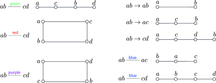
Figure 1: relations for $e_{1},e_{2}\in K(L)$.

Proof.

We only need to show $e_{1}$ and $e_{2}$ has one of the relations. The uniqueness obviously follows Fact 2.

When $|e_{1}\cap e_{2}|=2$, obviously (o.1) happens. When $|e_{1}\cap e_{2}|=1$, write $e_{1}=\{a,b\}$ and $e_{2}=\{a,c\}$. Since $c\in\overline{ac}=\overline{ab}=L$, the set {a, b, c} is collinear, one of $[bac]$, $[acb]$, and $[abc]$ happens. The first situation is (b.1), the second is (o.2), and the last does not happen since we assumed $\rho(e_{1})\geq\rho(e_{2})$.

Finally, $|e_{1}\cap e_{2}|=0$. Write $e_{1}=\{a,b\}$, $e_{2}=\{c,d\}$. Since $\{c,d\}\subseteq\overline{cd}=\overline{ab}=L$, both $\{a,b,c\}$ and $\{a,b,d\}$ are collinear. Similarly, $\{a,c,d\}$ and $\{b,c,d\}$ are collinear. Since $\rho(a,b)\geq\rho(c,d)$, we may choose the letters so that either $\rho(a,b)$ is one of the largest distances among the fours points, or $\rho(a,d)$ is one of the largest. We discuss two cases.

Case 1. $\rho(a,b)$ is one of the largest distances among $\{a,b,c,d\}$. Since $\{a,b,c\}$ and $\{a,b,d\}$ are both collinear, both $c$ and $d$ are between $a$ and $b$, i.e., $[acb]$ and $[adb]$. We may choose the letters so that $\rho(a,c)\leq\rho(a,d)$. Let $\rho(a,c)=x$, $\rho(a,d)=y$, $0<x\leq y$. Because $a\in\overline{ab}=\overline{cd}=L$, we have $[adc]$, $[acd]$, or $[cad]$. $[adc]$ contradicts the assumption $\rho(a,c)\leq\rho(a,d)$.

Case 1.1. $[acd]$. Fact 1 (c) together with $[adb]$ imply $[acdb]$; and this is (o.3).

Case 1.2. $[cad]$. We have $\rho(c,d)=x+y$. Let $x^{\prime}=\rho(b,d)$ and $y^{\prime}=\rho(b,c)$. By the assumption $[acb]$ and $[adb]$, we have

$$x+y^{\prime}=\rho(a,c)+\rho(c,b)=\rho(a,b)=\rho(a,d)+\rho(b,d)=y+x^{\prime}.$$ (2)

$x\leq y$ implies $x^{\prime}\leq y^{\prime}$. $\{b,c,d\}$ is collinear, so $[dcb]$, $[cdb]$, or $[cbd]$. $[dcb]$ contradicts the fact $x^{\prime}\leq y^{\prime}$. $[cdb]$, together with $[acb]$ and Fact 1 (c) implies $[acdb]$; this is (o.3). Finally, $[cbd]$ implies $x+y=\rho(c,d)=x^{\prime}+y^{\prime}$, together with (2), we have $x=x^{\prime}$ and $y=y^{\prime}$; this is situation (p).

Case 2. $\rho(a,d)$ is one of the largest distances among $\{a,b,c,d\}$. Since every triple in $\{a,b,c,d\}$ is a collinear set, we have $[abd]$ and $[acd]$. Now, we discuss on the collinear set $\{a,b,c\}$.

Case 2.1. $[abc]$. Together with $[acd]$ and Fact 1 (c) we have $[abcd]$; this is situation (b.2).

Case 2.2. $[acb]$. Together with $[abd]$ and Fact 1 (c) we have $[acbd]$; this is situation (g).

Case 2.3. $[bac]$. Let $x=\rho(a,b)$ and $y=\rho(a,c)$, then $\rho(b,c)=x+y$. Let $x^{\prime}=\rho(c,d)$ and $y^{\prime}=\rho(b,d)$. $[abd]$ and $[acd]$ imply

$$x+y^{\prime}=\rho(a,b)+\rho(b,d)=\rho(a,d)=\rho(a,c)+\rho(c,d)=x^{\prime}+y.$$ (3)

Note that $\{b,c,d\}$ is collinear. If $[bcd]$, together with $[bac]$ and Fact 1 (c) we have $[bacd]$ contradicts the maximality assumption of Case 2. The same happens when $[cbd]$. So we have $[cdb]$, so

$$\rho(b,c)=x+y=x^{\prime}+y^{\prime}.$$

Together with (3) imply $x=x^{\prime}$ and $y=y^{\prime}$. It is easy to see this is situation (r). ∎

Next, we define a graph on the pairs of points. Throughout the paper we use points for the elements of the metric space, and vertices for the vertices of the graph, so each vertex is a pair of points.

Definition 5.

Define a relation $\mathcal{P}_{L}=(K(L),\preccurlyeq)$ as $e_{2}\preccurlyeq e_{1}$ if and only if $e_{1}$ and $e_{2}$ satisfy one of the ordered relations (o) in Fact 4.

Define a coloured graph $\mathcal{G}_{L}$ on $K(L)$, $e_{1}$ and $e_{2}$ has an edge with colour blue (respectively, green, red, purple) whenever they have the blue (respectively, green, red, purple) relation as in Fact 4, and we denote this by $e_{1}\sim_{b}e_{2}$ (respectively, $e_{1}\sim_{g}e_{2}$, $e_{1}\sim_{r}e_{2}$, $e_{1}\sim_{p}e_{2}$).

By Fact 1, it is easy to check that $\mathcal{P}_{L}$ is a partially ordered set (poset). Now we give a partition of $K(L)$.

Definition 6.

For $e\in K(L)$, define $\ell(e)$ be the length of the longest chain in the poset $\mathcal{P}_{L}$ with $e$ as its maximum element.

For a positive integer $k$, define

$$\mathcal{P}_{L}^{(k)}=\ell^{-1}(k)=\{e\in K(L):\ell(e)=k\}.$$

and $\mathcal{G}_{L}^{(k)}$ be the (coloured) induced subgraph of $\mathcal{G}_{L}$ on $\mathcal{P}_{L}^{(k)}$.

Let $h(L)$ be the largest integer $k$ for which $\mathcal{P}_{L}^{(k)}\neq\emptyset$. This is the height of $\mathcal{P}_{L}$.

It is a well known fact in partially ordered sets that

Fact 5.

For each positive integer $k$, $\mathcal{P}_{L}^{(k)}$ is an antichain.

Proof.

Suppose $e_{1}\neq e_{2}\in\mathcal{P}_{L}^{(k)}$ and $e_{1}\preccurlyeq e_{2}$. By definition $\ell(e_{1})=\ell(e_{2})=k$. There is a chain $C$ with maximum element $e_{1}$ and $|C|=k$. But then $C\cup\{e_{2}\}$ is a chain with maximum element $e_{2}$ and size $k+1$, contradicts the fact $\ell(e_{2})=k$. ∎

Consequently, since Fact 4 tells us that any two elements in $K(L)$ either has the ordered relation or one of the coloured edges, we have

Fact 6.

For every integer $k$ ($1\leq k\leq h(L)$), the graph $\mathcal{G}_{L}^{(k)}$ is a complete graph (with coloured edges).

We also note that, it is clear from Fact 4 and Fact 1 that

Fact 7.

For every $ab\in\mathcal{P}_{L}^{(k)}$, there are at least $k-1$ inner points collinear with $a$ and $b$, i.e., there are distinct points $x_{1},x_{2},\dots,x_{k-1}$ in $V\setminus\{a,b\}$ such that

$$[ax_{1}x_{2}\dots x_{k-1}b].$$

3 The structure of $K(L)$

Definition 7.

We call an element $e\in K(L)$ purple if $e\sim_{p}f$ for some $f\in K(L)$, and denote $D(L)$ the set of all the purple elements; call an element $e\in K(L)$ red if $e\sim_{r}f$ for some $f\in K(L)$, and denote $U(L)$ the set of all the red elements.

Fact 8.

For a red element $e=\{a,b\}\in U(L)$, no point (other than $a$ and $b$) in $V$ is between $a$ and $b$; furthermore, $e$ is a minimal element in the poset $\mathcal{P}_{L}$.

Proof.

Indeed, suppose $[avb]$. Let $x_{1}=\rho(a,v)$, $x_{2}=\rho(v,b)$, and $x=x_{1}+x_{2}=\rho(a,b)$. Pick an element $f\in K(L)$ such that $e\sim_{r}f$. By Fact 4, $[cad]$ and $[acd]$, together with $[avb]$ we have $[vac]$ and $[vbd]$. Also by Fact 4, $\rho(a,c)=\rho(b,d)=y$, $\rho(c,d)=x$. We have

$$\begin{split}[vac]\Rightarrow&\rho(v,c)=x_{1}+y,\\ [vbd]\Rightarrow&\rho(v,b)=x_{2}+y,\\ &\rho(c,d)=x.\end{split}$$

It is easy to see that the sum of any two of the distances among $\{v,c,d\}$ is larger than the third. So $v\not\in\overline{cd}=L$. But $[avb]$ implies $v\in\overline{ab}=L$, a contradiction.

It immediately follows that $e$ is a minimal element in $\mathcal{P}_{L}$ — were there $f\in K(L)$, $f\neq e$ and $f\preccurlyeq e$, by Fact 4 (o) there would be another point in $L$ between $a$ and $b$. ∎

Fact 9.

For a purple element $e=\{a,b\}\in D(L)$, every point in $L$ (other than $a$ and $b$) is between $a$ and $b$, i.e., for every $v\in L$, we have $[avb]$.

Proof.

Since $e$ is purple, there is $f=\{c,d\}\in K(L)$ such that $e\sim_{p}f$. Suppose $v\in L=\overline{ab}$ and $v$ is not between $a$ and $b$. Without loss of generality, $[abv]$. By Fact 4 (p), we have $[acb]$ and $[adb]$; then by Fact 1 we have $[cbv]$ and $[dbv]$; also Fact 4 (p) tells us $[cbd]$, so, by Fact 3, $\{v,c,d\}$ is not collinear, contradicts the fact $v\in L=\overline{cd}$. ∎

Fact 10.

When the set of purple elements $D(L)\neq\emptyset$, we have

(a) $D(L)$ is the set of all maximal elements in the poset $\mathcal{P}_{L}$;

(b) For any $e\neq f\in D(L)$, $e\sim_{p}f$;

(c) For any $e\in D(L)$ and $f\in K(L)\setminus D(L)$, $f\preccurlyeq e$.

(d) $D(L)=\mathcal{P}_{L}^{(h(L))}$, the last level of the poset $\mathcal{P}_{L}$.

Proof.

We first note that,

$$\forall e\in D(L)\forall f\in K(L),f\preccurlyeq e\;\;\text{or}\;\;e\sim_{p}f.$$ (4)

This can be seen by observing Fact 4. $e$ and $f$ have one of the relations, but anything other than the two listed in (4) leads to a contradiction with Fact 9.

Denote $M$ the set of maximal elements in $\mathcal{P}_{L}$.

(a). For every $e\in D(L)$, by (4), there cannot exist $f\neq e$, $f\in K(L)$, such that $e\preccurlyeq f$, so $e\in M$. Thus we have $D(L)\subseteq M$. On the other hand, since $D(L)\neq\emptyset$, pick some $e^{*}\in D(L)$. Suppose $f$ is any other maximal element so $f\preccurlyeq e$ does not hold. By (4), $e\sim_{p}f$, thus $f$ is purple by the definition. Therefore, $M\subseteq D(L)$.

(b). Now we have both $e$ and $f$ are maximal elements, so they are not comparable, and (4) implies $e\sim_{p}f$.

(c). Since $f$ is not purple, $e\not\sim_{p}f$, so (4) implies $f\preccurlyeq e$.

(d). If $D(L)=K(L)$, no two elements are comparable by (a), and we have $\ell(e)=1$ for all $e\in K(L)$; so $h(L)=1$ and $\mathcal{P}_{L}^{(1)}=K(L)=D(L)$. Otherwise, consider a longest chain without a purple element

$$C=(e_{1},e_{2},\dots,e_{t}).$$

Given any non-purple element $f\in K(L)$, (c) implies that the longest chain with $f$ as its maximum element does not contain purple elements, so we have

$$\forall f\in K(L)\setminus D(L),\;\;\ell(f)\leq t.$$ (5)

On the other hand, for every $e\in D(L)$, (a) implies the longest chain with $f$ as its maximum element does not contain any other purple elements, so $\ell(e)\leq t+1$; but $C\cup\{e\}$ is a chain, so

$$\forall e\in K(L),\;\;\ell(e)=t+1.$$ (6)

(5) and (6) imply $h(L)=t+1$ and $D(L)=\mathcal{P}_{L}^{(h(L))}$. ∎

Now we turn to the study $\mathcal{P}_{L}^{(k)}$ for $2\leq k\leq h(L)-1$. By Facts 8 and 10, there are no red nor blue elements in such levels; Fact 6 implies that $\mathcal{G}_{L}^{(k)}$ is a complete graph with blue and green edges.

Definition 8.

For a line $L$ and $2\leq k\leq h(L)-1$, $\mathcal{R}_{L}^{(k)}$ is the green sub-graph of $\mathcal{G}_{L}^{(k)}$, it has the vertex set $\mathcal{P}_{L}^{(k)}$ and has all the green edges of $\mathcal{G}_{L}^{(k)}$. Denote $Q_{L}^{(k)}$ the set of isolated vertices in $\mathcal{R}_{L}^{(k)}$, denote $c_{L}(k)$ the number of connected components of size at least 2 in $\mathcal{R}_{L}^{(k)}$, we call them the green components in level $k$, denote $P_{L}^{(k,i)}$ ($i=1,2,\dots,c_{L}(k)$) the vertex set for each green component.

For every subset $U\subseteq\mathcal{P}_{L}^{(k)}$, denote $V(U)\subseteq V$ the union of elements (each is a pair of points in $V$) of $U$, i.e., all the endpoints of generating pairs of $L$ in $U$.

Fact 11.

For every $2\leq k\leq h(L)-1$, $\left|Q_{L}^{(k)}\right|\leq n/(k-1)$.

Proof.

Fact 7 implies that each element in $Q_{L}^{(k)}$ has $k-1$ “inner” points, we just need to show that these inner points are all distinct. Suppose $ab,cd\in Q_{L}^{(k)}$ and $[axb]$, $[cyd]$, we want to show that $x\neq y$. Indeed, $ab$ and $cd$ are isolated vertices in $\mathcal{R}_{L}^{(k)}$, so $ab\sim_{b}cd$. By the categorization in Fact 4, We have either $[axbcyd]$, or, in the special case of $d=a$, $[bxayc]$. It is clear in both cases $x\neq y$. ∎

4 The structure of a green component

In this section, we fix a line $L$, an index $k$ ($2\leq k\leq h(L)-1$), denote $\mathcal{U}=\mathcal{P}_{L}^{(k)}$, and denote the green subgraph $\mathcal{R}_{L}^{(k)}$ by $\mathcal{R}$.

Definition 9.

For a subset $\mathcal{W}\subseteq\mathcal{U}$, we call a permutation $\pi$ of the set of its endpoints $V(\mathcal{W})$ a collinear ordering for $\mathcal{W}$ if $\pi$ is a collinear sequence. For each pair $ab\in\mathcal{W}$, where $a$ comes before $b$ in $\pi$, we call $a$ the open point of $ab$, and $b$ the corresponding close point. Since any two pairs $ab,cd\in\mathcal{W}$ has either $ab\sim_{b}cd$ or $ab\sim_{g}cd$, all the open points are distinct; we call the sequence of open points, sorted by their position in $\pi$ from the earliest to the latest, the opening sequence of $\pi$.

Let $a$ be an open point and $b$ be its corresponding close point, and $v$ be a point in $L=\overline{ab}$. We say $v$ is on the left side of $a$ in $\pi$ if $[vab]$, otherwise $v$ is on the right side of $a$. We say $v$ is on the left side of $b$ in $\pi$ if $[vab]$ or $[avb]$, otherwise $v$ is on the right side of $b$.

We will prove the existence of a collinear ordering for every connected subgraph of $\mathcal{R}$. Before this, we first discuss some properties of such an ordering if one exists, as we will need them in the inductive proof.

Lemma 1 analyzes the open and close points on a collinear ordering, and the relation of a single point $v\in L$ to the open-close pairs. In turn, Lemma 3 gives the shape of the line $L$ with respect to a collinear ordering. (See Figure 2.)

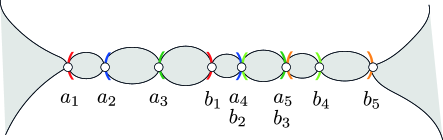
Figure 2: The shaded area consists all points of $L$. In a collinear ordering, $a_{1},a_{2},\dots,a_{5}$ are the open points, $b_{1},b_{2},\dots,b_{5}$ are corresponding close points. $V=\overline{a_{i}b_{i}}$ for all $i=1,2,3,4,5$.

Lemma 1.

Let $H$ be a connected subgraph of $\mathcal{R}$ with order at least 2, $\pi$ a collinear ordering for the vertex set of $H$, with $(a_{1},a_{2},\dots,a_{t})$ as its opening sequence; let $b_{i}$ be the corresponding close point to $a_{i}$ $i=1,2,\dots,t$. Then

(a) The $b_{i}$’s are distinct and their order in $\pi$, from left to the right, is $b_{1},b_{2},\dots,b_{t}$;

(b) $a_{i}b_{i}\sim_{g}a_{i+1}b_{i+1}$ for every $1\leq i<t$ and their order on $\pi$ is $a_{i},a_{i+1},b_{i},b_{i+1}$, and these four points are distinct;

(c) For every point $v\in L$, either $v$ appears on $\pi$, or $\pi$ has a partition $\pi=\sigma\circ\tau$ such that $v$ is on the right side of all points in $\sigma$ and on the left side of all points in $\tau$. (Here $\sigma$ and $\tau$ can be the empty sequence.)

Proof.

(a). We only need to show $b_{i}$ comes strictly before $b_{i+1}$ for $1\leq i<t$. Assume $b_{i+1}$ comes before $b_{i}$ or $b_{i+1}=b_{i}$, then $a_{i}b_{i}$ and $a_{i+1}b_{i+1}$ have one of the ordered relations in Fact 4, contradicts the fact that they have blue or green relation.

(b). By (a) and the definition of open and close points, among the four points, $a_{i}$ is the first and $b_{i+1}$ is the last. Now if $b_{i}$ is before $a_{i+1}$ or $b_{i}=a_{i+1}$, $a_{j}\geq b_{k}$ for all $j>i$ and $k\leq i$, so all the edges between $\{a_{k}b_{k}:k\leq i\}$ and $\{a_{j}b_{j}:j>i\}$ are blue, contradicts the fact that $H$ is a connected by green edges.

(c). Suppose $v\in L$ but does not appear on $\pi$. We only need to show there cannot be two adjacent points $x$ and $y$ in $\pi$ such that $x$ is to the left of $y$, $v$ is on the left side of $x$ but on the right side of $y$. Suppose the contrary and assume $x$ and $y$ is the earliest such a pair. We have the following cases. (Note that since a close point can be the open point for another pair, the cases might overlap.)

Case 1. Both $x$ and $y$ are open points. We have $x=a_{i}$ and $y=a_{i+1}$ for some $1\leq i<t$. By (b) we have

$$[a_{i}a_{i+1}b_{i}b_{i+1}]$$ (7)

By definition, $v$ is on the left side of $x=a_{i}$, so we have

$$[va_{i}b_{i}]$$ (8)

(7) and (8) imply

$$[va_{i}a_{i+1}b_{i}].$$ (9)

$v$ is on the right side of $y=a_{i+1}$, so $[a_{i+1}vb_{i+1}]$ or $[a_{i+1}b_{i+1}v]$. However, $[a_{i+1}vb_{i+1}]$ and $[a_{i}a_{i+1}b_{i+1}]$ in (7) imply $[a_{i}a_{i+1}vb_{i+1}]$, thus $[a_{i}a_{i+1}v]$, contradicts $[va_{i}a_{i+1}]$ in (9); and $[a_{i+1}b_{i+1}v]$ and $[a_{i+1}b_{i}b_{i+1}]$ in (7) imply $[a_{i+1}b_{i}b_{i+1}v]$, thus $[a_{i+1}b_{i}v]$, contradicts $[va_{i+1}b_{i}]$ in (9).

Case 2. Both $x$ and $y$ are close points. This is completely similar to the previous case. Or, we can reverse $\pi$ and reduce this to the previous case.

Case 3. $x=a_{j}$ is an open point and $y=b_{i}$ is a close point. Since $a_{j}$ and $b_{i}$ are adjacent in $\pi$, by (a) and (b), we have $i<j$ and

$$[a_{i}a_{j}b_{i}b_{j}]$$ (10)

on $\pi$. $v$ is on the left side of $x=a_{j}$ and on the right side of $y=b_{i}$, by definition, we have

$$[va_{j}b_{j}]\;\;\mbox{and}\;\;[a_{i}b_{i}v].$$ (11)

The first item in (11) and $[a_{j}b_{i}b_{j}]$ in (10) imply $[va_{j}b_{i}b_{j}]$, thus

$$[va_{j}b_{i}].$$ (12)

The second item in (11) and $[a_{i}a_{j}b_{i}]$ in (10) imply $[a_{i}a_{j}b_{i}v]$, thus $[a_{j}b_{i}v]$, contradicts (12).

Case 4. $x=b_{i}$ is a close point and $y=a_{j}$ is an open point. Since $x$ and $y$ are adjacent in $\pi$, and by (a) and (b), it is easy to see $i+1<j$, and we have

$$[a_{i}a_{i+1}b_{i}a_{j}b_{i+1}b_{j}].$$ (13)

Now $v$ is on the left side of $x=b_{i}$ and on the right side of $y=a_{j}$, we have

$$\begin{split}[va_{i}b_{i}]\;\;&\mbox{or}\;\;[a_{i}vb_{i}]\\ &\mbox{and}\\ [a_{j}b_{j}v]\;\;&\mbox{or}\;\;[a_{j}vb_{j}].\end{split}$$ (14)

$[a_{i}vb_{i}]$ and $[a_{i}b_{i}a_{j}b_{j}]$ in (13) imply $[a_{i}vb_{i}a_{j}b_{j}]$, thus $[va_{j}b_{j}]$, contradicts the fact that $v$ is on the right side of $a_{j}$.

$[a_{j}vb_{j}]$ and $[a_{i}b_{i}a_{j}b_{j}]$ in (13) imply $[a_{i}b_{i}a_{j}vb_{j}]$, thus $[a_{i}b_{i}v]$, contradicts the fact that $v$ is on the left side of $b_{i}$.

So, (14) becomes

$$[va_{i}b_{i}]\;\;\mbox{and}\;\;[a_{j}b_{j}v]$$ (15)

The first item above means $v$ is on the left side of $a_{i}$, and by the minimality of $x$, $v$ is on the left side of all points in $\pi$ between $a_{i}$ and $b_{i}$, in particular, $v$ is on the left side of $a_{i+1}$, i.e., $[va_{i+1}b_{i+1}]$. This, together with $[a_{i+1}a_{j}b_{i+1}]$ in (13), implies $[va_{i+1}a_{j}b_{i+1}]$, thus

$$[va_{j}b_{i+1}].$$ (16)

The second item in (15) and $[a_{j}b_{i+1}b_{j}]$ in (13) imply $[a_{j}b_{i+1}b_{j}v]$, thus $[a_{j}b_{i+1}v]$, contradicts (16). ∎

The following lemma is well-known in graph theory.

Lemma 2.

Every connected graph $G$ with order at least 2 has a vertex that is not a cut point, i.e., $G-v$ is still connected.

Proof.

Consider a spanning tree $T$ of $G$. Being a tree with at least two vertices, $T$ has at least two leaves. Any leaf $v$ of $T$ has the property that $T-v$ is connected, so $G-v$ is connected. ∎

Lemma 3.

For every connected subgraph $H$ of $\mathcal{R}$, a collinear ordering $\pi$ for the vertex set of $H$, and every point $v\in L$ that does not appear on $\pi$, $v$ can be inserted into $\pi$ in a unique way to form a collinear sequence.

Proof.

The uniqueness of the insertion position follows from Fact 2. We show the existence of the position by induction on the order of $H$. The base case when $H$ has one vertex $e=ab$ is clear — since $v\in L=\overline{ab}$, we have $[vab]$, $[avb]$, or $[abv]$. Now assume $H$ has order at least two and the statement holds for every connected subgraph of $H$ with a smaller order. Let $(a_{1},a_{2},\dots,a_{t})$ be the opening sequence for $\pi$, and $b_{i}$ be the corresponding close point to $a_{i}$. Let $\sigma$ and $\tau$ be the partition of $\pi$ assured by Lemma 1 (c).

Case 1. $\sigma$ is the empty sequence.

So, $\tau=\pi$ and $v$ is on the left side of all the points (especially all the open points) in $\pi$. Thus,

$$[va_{i}b_{i}],\;\;\forall 1\leq i\leq t.$$ (17)

By Lemma 1 (b), $H-a_{t}b_{t}$ is connected. The sub-sequence $\pi^{\prime}$ of $\pi$ formed by $\{a_{1},b_{1},a_{2},b_{2},\dots,a_{t-1},b_{t-1}\}$ is a collinear ordering for $H-a_{t}b_{t}$. Thus, the inductive hypothesis assures that $v$ can be inserted into $\pi^{\prime}$ to form a collinear sequence $\pi^{\prime\prime}$. Since $v$ is on the $a_{1}$-side of $\{a_{1},b_{1}\}$, we conclude that

$$\pi^{\prime\prime}=(v)\circ\pi^{\prime} b_{t-1}$$ is a collinear sequence ends with . (18)

By Lemma 1 (b), $[a_{t}b_{t-1}b_{t}]$, together with $[va_{t}b_{t}]$ in (17), we have $[va_{t}b_{t-1}b_{t}]$, so $[vb_{t-1}b_{t}]$, then, by (18) and Fact 1 (d),

$$(v)\circ\pi^{\prime}\circ(b_{t})$$ is a collinear sequence. (19)

By Lemma 1 (a) and (b), $a_{t}$ is not the first point, nor among the last two points in $\pi$, so either $a_{t}$ appears on $\pi^{\prime}$, or there are consecutive points $x$ and $y$ on $\pi^{\prime}$ such that $[xa_{t}y]$, then, by Fact 1 (d), it can be inserted into the sequence in (19) to form a collinear sequence. In either case, we have $\{v,a_{1},b_{1},\dots,a_{t},b_{t}\}$ is a collinear set. We choose a collinear sequence $\pi^{*}$ for the set where $a_{1}$ comes before $a_{2}$ from Fact 2. Again by Fact 2, $\pi$ must be a subsequence of $\pi^{*}$, and since $[va_{1}b_{1}]$ in (17), so $\pi^{*}=(v)\circ\pi$.

Case 2. $\tau$ is the empty sequence. This is symmetric to Case 1. In fact we can reverse $\pi$ and reduce this to Case 1.

Case 3. Both $\sigma$ and $\tau$ are non-empty. Let $x$ be the last point in $\sigma$ and $y$ be the first point of $\tau$. By Fact 1 (d), it is enough to show $[xvy]$.

Case 3.1. Both $x$ and $y$ are open points. We may assume $x=a_{i}$ and $y=a_{i+1}$ for some $1\leq i<t$. By Lemma 1 (b) we have

$$[a_{i}a_{i+1}b_{i}b_{i+1}]$$ (20)

Since $v$ is on the left side of $y=a_{i+1}$, we have $[va_{i+1}b_{i+1}]$, together with (20), we get $[va_{i+1}b_{i}b_{i+1}]$ thus

$$[va_{i+1}b_{i}]$$ (21)

Since $b_{i}$ comes after $a_{i+1}$ in $\pi$, so it is in $\tau$; together with the fact $a_{i}$ is in $\sigma$ we have $[a_{i}vb_{i}]$, this, together with (21), implies $[a_{i}va_{i+1}b_{i}]$, so $[a_{i}va_{i+1}]$, i.e., $[xvy]$.

Case 3.2. Both $x$ and $y$ are close points. This is completely symmetric to the previous sub-case. Again, we may reverse $\pi$ and reduce to the previous one.

Case 3.3. $x=a_{j}$ is an open point and $y=b_{i}$ is a close point. In $\pi$, $x$ and $y$ are adjacent; $a_{i}$ occurs before $b_{i}$, so it is before $a_{j}$, $b_{j}$ occurs after $a_{j}$, so it is after $b_{i}$. From here we may conclude

$$[a_{i}a_{j}b_{i}b_{j}]\Rightarrow\rho(a_{i},b_{i})+\rho(a_{j},b_{j})=\rho(a_{i},b_{j})+\rho(a_{j},b_{i}),$$ (22)

$$a_{i}\in\sigma,b_{i}\in\tau\Rightarrow[a_{i}vb_{i}]\Rightarrow\rho(a_{i},b_{i})=\rho(a_{i},v)+\rho(v,b_{i}),$$ (23)

and

$$a_{j}\in\sigma,b_{j}\in\tau\Rightarrow[a_{j}vb_{j}]\Rightarrow\rho(a_{j},b_{j})=\rho(a_{j},v)+\rho(v,b_{j}).$$ (24)

Add the conclusions in (23) and (24), then compare with the conclusion in (22) we have

$$(\rho(a_{i},v)+\rho(v,b_{j}))+(\rho(a_{j},v)+\rho(v,b_{i}))=\rho(a_{i},b_{j})+\rho(a_{j},b_{i}).$$ (25)

But in every metric space,

$$\rho(a_{i},v)+\rho(v,b_{j})\geq\rho(a_{i},b_{j}),\;\;\rho(a_{j},v)+\rho(v,b_{i})\geq\rho(a_{j},b_{i}).$$ (26)

(25) means both inequalities in (26) must take the equal sign. In particular, $[a_{j}vb_{i}]$, i.e., $[xvy]$.

Case 3.4. $x=b_{i}$ is a close point and $y=a_{j}$ is an open point. In $\pi$, $x$ and $y$ are adjacent, it is easy to conclude

$$(a_{i},a_{i+1},b_{i},a_{j},b_{i+1},b_{j})\;\;\mbox{is a sub-sequence of $\pi$}.$$ (27)

$a_{i},a_{i+1},b_{i}$ are in $\sigma$ and $a_{j},b_{i+1},b_{j}$ are in $\tau$, so we have

$$[a_{i}b_{i}v],[a_{i+1}vb_{i+1}],\;\mbox{and}\;[va_{j}b_{j}].$$ (28)

$[a_{i}a_{i+1}b_{i}]$ reads from (27), and with the first item in (28), we get $[a_{i}a_{i+1}b_{i}v]$, so $[a_{i+1}b_{i}v]$, together with the second item in (28) we get

$$[a_{i+1}b_{i}vb_{i+1}].$$ (29)

$[a_{j}b_{i+1}b_{j}]$ reads from (27), and with the last item in (28), we get $[va_{j}b_{i+1}b_{j}]$, so $[va_{j}b_{i+1}]$. $[va_{j}b_{i+1}]$ and (29) implies $[a_{i+1}b_{i}va_{j}b_{i+1}]$, so $[xvy]$. ∎

Definition 10.

For every connected subgraph $H$ of $\mathcal{R}$, a collinear ordering $\pi$ for the vertex set of $H$, and every point $v\in L$ that does not appear on $\pi$, we call $v$ outside $H$ if $(v)\circ\pi$ or $\pi\circ(v)$ is a collinear sequence, otherwise call it inside $H$.

Lemma 4.

The vertex set of every connected subgraph of $\mathcal{R}$ has a collinear ordering.

Proof.

We prove by induction on the order of the subgraph $H$. The base case when $H$ has just one vertex is obvious. Now assume every connected subgraph of $H$ with a smaller order has a collinear ordering.

By Lemma 2, there is a vertex $e=ab$ in $H$ such that $H-e$ is connected. By the inductive hypothesis, there is a collinear ordering $\pi$ for $H-e$. By the connectedness of $H$, there is another vertex $f=cd$ such that $ab\sim_{g}cd$, we may assume $[acbd]$. By Lemma 3, $b$ can be inserted into $\pi$ to form a collinear sequence $\pi^{\prime}$. Since $[cbd]$, their order in $\pi^{\prime}$ from left to the right is $c$, $b$, and $d$. Let $x$ and $y$ be the left and right neighbour of $b$ in $\pi^{\prime}$, respectively. $x$ and $y$ are adjacent in $\pi$, and both $x$ and $y$ are contained in the range between $c$ and $d$ in $\pi$, inclusively.

By Lemma 3, $a$ can be inserted into $\pi$ to form a collinear sequence $\pi^{\prime\prime}$. $a$ can not be inserted into $\pi$ between $x$ and $y$ to form a collinear sequence, otherwise $a$ is between $c$ and $d$, contradicts the fact $[acd]$. So $x$ and $y$ is still adjacent in $\pi^{\prime\prime}$. From $\pi^{\prime}$ we see $[xby]$, so $b$ can be inserted into $\pi^{\prime\prime}$ between $x$ and $y$ to form a collinear ordering. ∎

Definition 11.

By Lemma 4 and Fact 2, the vertex set of every green component $\mathcal{C}$ in level $k$ has exactly two collinear orderings reverse each other. We call one of them the standard collinear ordering for $\mathcal{C}$.

5 Proof of the main theorem

Our first lemma is a main ingredient in [1], we prove it here for completeness.

Lemma 5.

If $t$ distinct points $v_{1},v_{2},\dots,v_{t}$ satisfy $[v_{1}v_{2}\dots v_{t}]$ in a metric space without a universal line, then there are at least $t$ distinct lines.

Proof.

For every $i$ such that $1\leq i<t$, pick a point $u_{i}\in V\setminus\overline{v_{i}v_{i+1}}$. (It is possible that $u_{i}=u_{j}$ for $i\neq j$.) We claim that $L_{i}=\overline{u_{i}v_{i}}$ ($i=1,2,\dots,t-1$) are all distinct lines. First of all, $u_{i}\not\in\overline{v_{i}v_{i+1}}$, so $\{u_{i},v_{i},v_{i+1}\}$ is not collinear, so $v_{i+1}\not\in L_{i}$ for each $i$. For $1\leq i<j<t$, suppose $L_{i}=L_{j}$, so $\{u_{i},v_{i},v_{j}\}$ is collinear. By Fact 1, $[u_{i}v_{i}v_{j}]$ and $[v_{i}v_{i+1}v_{j}]$ imply $[u_{i}v_{i}v_{i+1}]$; $[v_{i}v_{j}u_{i}]$ and $[v_{i}v_{i+1}v_{j}]$ also imply $[u_{i}v_{i}v_{i+1}]$; finally, $[v_{i}u_{i}v_{j}]$ and $[v_{i}v_{j}v_{j+1}]$ imply $[v_{i}u_{i}v_{j+1}]$, so $v_{j+1}\in L_{i}=L_{j}$, this means $\{v_{j+1},v_{j},u_{j}\}$ is collinear, contradicts the fact that $u_{j}\not\in\overline{v_{j}v_{j+1}}$. ∎

Definition 12.

Let $L$ be a line in a metric space $(V,\rho)$ without a universal line, $(2\leq k\leq h(L)-1)$, let $\mathcal{C}$ be a green component in level $k$ of $\mathcal{P}_{L}$, and let $(a_{1},a_{2},\dots,a_{t})$ be the opening sequence of $\mathcal{C}$’s standard collinear ordering. For every $i$ such that $1\leq i<t$, $\overline{a_{i}a_{i+1}}\neq V$, so we can pick (any) $u_{i}\in V$ such that $\{u_{i},a_{i},a_{i+1}\}$ is not collinear. Set $L_{i}=\overline{u_{i}a_{i+1}}$ so $a_{i}\not\in\overline{L_{i}}$.

We call $u_{i}$ the $i$-th special point and $L_{i}$ the $i$-th special line with respect to the green component $\mathcal{C}$.

Note that the $u_{i}$’s may well be repeated for different index $i$. However, now we are going to show that the $L_{i}$’s are distinct.

Lemma 6.

For a line $L$ in a metric space $(V,\rho)$ without a universal line, any level $k$ $(2\leq k\leq h(L)-1)$, and any green component $\mathcal{C}$ in level $k$ of $\mathcal{P}_{L}$, all the special lines with respect to $\mathcal{C}$ are distinct.

Proof.

Denote $(a_{1},a_{2},\dots,a_{t})$ the opening sequence of the standard collinear ordering of $\mathcal{C}$; denote $u_{i}$ the $i$-th special element and $L_{i}$ the $i$-th special line $\overline{u_{i}a_{i+1}}$. Suppose the contrary that there are $i<j$ such that $L_{i}=L_{j}$. So $a_{j+1}\in L_{j}=L_{i}$, this means $\{u_{i},a_{i+1},a_{j+1}\}$ is collinear.

Case 1. $[a_{i+1}u_{i}a_{j+1}]$. In $\pi$ we have $[a_{i}a_{i+1}a_{j+1}]$, so $[a_{i}a_{i+1}u_{i}a_{j+1}]$, which implies $\{a_{i},a_{i+1},u_{i}\}$, contradicts the definition of $u_{i}$.

Case 2. $[u_{i}a_{i+1}a_{j+1}]$ (respectively $[a_{i+1}a_{j+1}u_{i}]$). In $\pi$ we have $[a_{i+1}a_{j}a_{j+1}]$ (no matter $i+1=j$ or not), so $[u_{i}a_{i+1}a_{j}a_{j+1}]$ (respectively $[a_{i+1}a_{j}a_{j+1}u_{i}]$), which implies $\{a_{j},u_{i},a_{i+1}\}$ is collinear, and $a_{j}\in L_{i}=L_{j}$, contradicts the definition of $L_{j}$. ∎

Lemma 7.

For a line $L$ in a metric space $(V,\rho)$ without a universal line, and any level $k$ $(2\leq k\leq h(L)-1)$, two special lines with respect to two different components in level $k$ of $\mathcal{P}_{L}$ are distinct.

Proof.

Let $(a_{1},a_{2},\dots,a_{t})$ be the opening sequence of the standard collinear ordering of the first component, $b_{i}$ be the corresponding close point to $a_{i}$; let $u_{i}$ be its $i$-th special element and $L_{i}=u_{i}a_{i+1}$ be the $i$-th special line. Let $\pi^{\prime}$ be a standard collinear ordering of the second component, with opening sequence $(a^{\prime}_{1},a^{\prime}_{2},\dots,a^{\prime}_{s})$, $b^{\prime}_{i}$ be the corresponding close point to $a^{\prime}_{i}$. By Lemma 1 (b), $[a_{i}a_{i+1}b_{i}]$. Since $a_{i}b_{i}$ and $a^{\prime}_{j}b^{\prime}_{j}$ are in different green components, we have $a_{i}b_{i}\sim_{b}a^{\prime}_{j}b^{\prime}_{j}$, together with $[a_{i}a_{i+1}b_{i}]$, we get

$$a_{i+1} \{a^{\prime}_{j}b^{\prime}_{j}\} j 1\leq j\leq s$$ is outside for every such that . (30)

Especially, $a_{i+1}$ does not appear on $\pi^{\prime}$. By Lemma 3, $a_{i+1}$ can be inserted into $\pi^{\prime}$ to get a collinear sequence $\pi^{*}$. If $a_{i+1}$ is not the first point on $\pi^{*}$, let $j$ be the largest index such that $a^{\prime}_{j}$ is earlier than $a_{i+1}$ in $\pi^{*}$. If $j<s$, by the maximality of $j$, $a^{\prime}_{j+1}$ is after $a_{i+1}$, and by Lemma 1 (b), $b^{\prime}_{j}$ is after $a^{\prime}_{j+1}$ so $a_{i+1}$ is between $a^{\prime}_{j}$ and $b^{\prime}_{j}$ in $\pi^{*}$, contradicts (30). So $j=s$, and by (30), $b^{\prime}_{s}$ is also earlier than $a_{i+1}$.

In a word, $a_{i+1}$ is either the first point or the last point in $\pi^{*}$. So $a_{i+1}$ is outside $\pi^{\prime}$. The lemma follows from the next stronger lemma. ∎

Lemma 8.

For a line $L$ in a metric space $(V,\rho)$ without a universal line, any level $k$ $(2\leq k\leq h(L)-1)$, and a green component $\mathcal{C}$ in level $k$, a special line with respect to $\mathcal{C}$ does not contain any point $v\in L$ but outside $\mathcal{C}$.

Proof.

Denote $\pi$ the standard collinear ordering of $\mathcal{C}$, $(a_{1},a_{2},\dots,a_{t})$ its opening sequence, and $b_{i}$ the close point corresponding to $a_{i}$; denote $u_{i}$ the $i$-th special element and $L_{i}=\overline{u_{i}a_{i+1}}$ the $i$-th special line.

Since $v$ is outside $\mathcal{C}$, either $(v)\circ\pi$ or $\pi\circ(v)$ is a collinear sequence. This means both $a_{i}$ and $b_{i+1}$ is collinear with $\{v,a_{i+1}\}$, and exactly one of them is between $v$ and $a_{i+1}$, the other is outside.

Assume the contrary $v\in L_{i}$, so $\{v,a_{i+1},u_{i}\}$ is collinear. Depending on whether $u_{i}$ is between $v$ and $a_{i+1}$ or not, by Fact 1 (c), there is one point in $x\in\{a_{i},b_{i+1}\}$ such that $\{x,u_{i},v,a_{i+1}\}$ is collinear, so $\{x,u_{i},a_{i+1}\}$ is collinear.

If $x=a_{i}$, $\{u_{i},a_{i},a_{i+1}\}$ is collinear, contradicts the definition of $u_{i}$. If $x=b_{i+1}$, $u_{i}\in\overline{a_{i+1}b_{i+1}}=L$; by Lemma 3, $u_{i}$ either appears on $\pi$ or can be inserted into $\pi$ to form a collinear sequence, so $\{u_{i},a_{i},a_{i+1}\}$ is collinear, again contradicts the definition of $u_{i}$. ∎

Lemma 9.

For a line $L$ a metric space $(V,\rho)$ without a universal line, and any level $k$ $(2\leq k\leq h(L)-1)$, all the special lines in level $k$ are distinct.

Proof.

This immediately follows from Lemmas 6 and 7. ∎

Now we prove the main theorem.

Proof.

(of Theorem 1) Denote $n=|V|$ and $m$ the number of distinct lines. The generating pairs defined in (1) gives a partition of $\binom{V}{2}$ into $m$ $K(L)$’s. If none of the parts $K(L)$ has size more than $4n^{4/3}$, we have the number of parts $m\geq\binom{n}{2}/(4n^{4/3})\in\Omega(n^{2/3})$.

Otherwise, there is a line $L$ with $|K(L)|\geq 4n^{4/3}$. Consider the poset $\mathcal{P}_{L}$.

If for every $k$ ($1\leq k\leq h(L)$) the antichain $\mathcal{P}_{L}^{(k)}$ has more than $n^{4/3}$ elements, by the handshake lemma, we have a point $v\in V$ such that $v$ is incident to more than $2n^{1/3}$ pairs, i.e., there are points $u_{1},u_{2},\dots,u_{d}$ in $V$, such that $vu_{i}\in\mathcal{P}_{L}^{(k)}$ for all $1\leq i\leq d$, and $d>2n^{1/3}$. For a pair of indices $i$ and $j$ where $1\leq i<j\leq d$, $\overline{vu_{i}}=\overline{vu_{j}}=L$ implies $\{v,u_{i},u_{j}\}$ is collinear, now the fact that $\mathcal{P}_{L}^{(k)}$ is an antichain implies $[u_{i}vu_{j}]$. Fact 3 implies that, for any $k\not\in\{i,j\}$, $\{u_{i},u_{j},u_{k}\}$ is not collinear. So $\overline{u_{i}u_{j}}$ contains both $u_{i}$ and $u_{j}$ but no any other point in $\{u_{1},u_{2},\dots,u_{d}\}$. Therefore we have $\binom{d}{2}\in\Omega(n^{2/3})$ distinct lines.

Now we may assume for each $1\leq k\leq h(L)$, we have $|\mathcal{P}_{L}{(k)}|\leq n^{4/3}$, this is in particular true for $k=1$ and $k=h(L)$. Since $|K(L)|\geq 4n^{4/3}$, we have

$$\sum_{k=2}^{h(L)-1}\left|\mathcal{P}_{L}{(k)}\right|=\sum_{k=2}^{h(L)-1}\left(\sum_{i=1}^{c_{L}(k)}\left|P_{L}^{(k,i)}\right|+\left|Q_{L}^{(k)}\right|\right)\geq 2n^{4/3}.$$ (31)

When $h(L)>n^{2/3}$, Fact 7 and Lemma 5 already imply $m\geq n^{2/3}$. Now we may assume $h(L)\leq n^{2/3}$.

By Fact 11,

$$\sum_{k=2}^{h(L)-1}\left|Q_{L}^{(k)}\right|\leq n\left(\frac{1}{4}+\frac{1}{5}+\dots+\frac{1}{n^{2/3}}\right)\leq n\ln n.$$

Subtracting from (31), we have, for large enough $n$,

$$\sum_{k=2}^{h(L)-1}\left(\sum_{i=1}^{c_{L}(k)}\left|P_{L}^{(k,i)}\right|\right)\geq 2n^{4/3}-n\ln n\geq n^{4/3}.$$

So there exists a $k$, $2\leq k\leq h(L)\leq n^{2/3}$, such that $\sum_{i=1}^{c_{L}(k)}\left|P_{L}^{(k,i)}\right|\geq n^{2/3}$. By definition, each $P_{L}^{(k,i)}$ has $|P_{L}^{(k,i)}|\geq 2$ and has exactly $|P_{L}^{(k,i)}|-1$ special lines. By Lemma 9, we have at least

$$\sum_{i=1}^{c_{L}(k)}\left(\left|P_{L}^{(k,i)}\right|-1\right)\geq\sum_{i=1}^{c_{L}(k)}\left(\left|P_{L}^{(k,i)}\right|/2\right)\geq\frac{n^{2/3}}{2}$$

distinct lines in the metric space. ∎

6 Discussion – the structure of two green components

The following structure of two green components can be proved by an induction. After simplification we do not need it in the proof of the main theorem, and we omit the proof.

Fact 12.

For every index $k$ such that $2\leq k\leq h(L)-1$, let $\pi$ and $\sigma$ be the standard ordering of two different green components in level $k$, there is a collinear sequence $\pi_{1}\circ\sigma_{1}$, where $\pi_{1}$ is either $\pi$ or $\pi^{R}$, and $\sigma_{1}$ is either $\sigma$ or $\sigma^{R}$.

References

- [1] P. Aboulker, X. Chen, G. Huzhang, R. Kapadia and C. Supko, Lines, betweenness and metric spaces, Discrete & Computational Geometry 56 (2016), 427 – 448.
- [2] X. Chen and V. Chvátal, Problems related to a de Bruijn - Erdős theorem, Discrete Applied Mathematics 156 (2008), 2101 – 2108.
- [3] N. G. De Bruijn and P. Erdős, On a combinatorial problem, Indagationes Mathematicae 10 (1948), 421 – 423.
- [4] F. Harary and R. C. Reed, Is the null-graph a pointless concept?, Graphs and Combinatorics: Proceedings of the Capital Conference on Graph Theory and Combinatorics at the George Washington University June 18–22, 1973 Springer Berlin Heidelberg (2006), 37 – 44.