Weak Lensing Reconstruction by Counting DECaLS Galaxies

Abstract

Alternative to weak lensing measurements through cosmic shear, we present a weak lensing convergence $\hat{\kappa}$ map reconstructed through cosmic magnification effect in DECaLS galaxies of the DESI imaging surveys DR9. This is achieved by linearly weighing $12$ maps of galaxy number overdensity in different magnitude bins of $grz$ photometry bands. The weight is designed to eliminate the mean galaxy deterministic bias, minimize galaxy shot noise while maintaining the lensing convergence signal. We also perform corrections of imaging systematics in the galaxy number overdensity. The $\hat{\kappa}$ map has $8365$ deg² sky coverage. Given the low number density of DECaLS galaxies, the $\hat{\kappa}$ map is overwhelmed by shot noise and the map quality is difficult to evaluate using the lensing auto-correlation. Alternatively, we measure its cross-correlation with the cosmic shear catalogs of DECaLS galaxies of DESI imaging surveys DR8, which has $8365$ deg² overlap in sky coverage with the $\hat{\kappa}$ map. We detect a convergence-shear cross-correlation signal with $S/N\simeq 10$. The analysis also shows that the galaxy intrinsic clustering is suppressed by a factor $\mathcal{O}(10^{2})$ and the residual galaxy clustering contamination in the $\hat{\kappa}$ map is consistent with zero. Various tests with different galaxy and shear samples, and the Akaike information criterion analysis all support the lensing detection. So is the imaging systematics corrections, which enhance the lensing signal detection by $\sim 30\%$. We discuss various issues for further improvement of the measurements.

I Introduction

Weak lensing, which probe directly the matter distribution of the Universe, provide powerful insight into dark energy, dark matter and gravity at cosmological scales (Bartelmann and Schneider, 2001a; Kilbinger, 2015a; Bartelmann and Schneider, 2001b; Hoekstra and Jain, 2008; Van Waerbeke et al., 2010; Fu and Fan, 2014; Kilbinger, 2015b). An effect of weak lensing is cosmic shear, which distorts shapes of distant galaxies. This signal can be extracted statistically from the galaxy images and has been the main target of current weak lensing studies. With large surveys, such as the on-going Dark Energy Survey (DES, Dark Energy Survey Collaboration et al., 2016), the Kilo-Degree Survey (KiDS, de Jong et al., 2013), and the Hyper Suprime-Cam Subaru Strategic Program survey(HSC-SSP, Aihara et al., 2018), cosmic shear contributed significantly to the precision cosmology (e.g., Hamana et al., 2020; Asgari et al., 2021; Giblin et al., 2021; Loureiro et al., 2022; Amon et al., 2022; Secco et al., 2022; Li et al., 2023).

Another weak lensing effect is cosmic magnification, which induces changes in the observed galaxy number density by magnifying the galaxy flux and resizing the solid angle of the sky patches (Blandford and Narayan, 1992; Bartelmann and Narayan, 1995). As the galaxy intrinsic alignment contaminates the cosmic shear signal, the galaxy intrinsic clustering contaminates the cosmic magnification signal. In observations, cosmic magnification is typically measured through cross correlations of two samples in the same patch of the sky but widely separated in redshift. Lenses include luminous red galaxies (LRGs) and clusters (e.g., Bauer et al., 2014; Bellagamba et al., 2019; Chiu et al., 2016, 2020). Sources at higher redshifts include quasars (Scranton et al., 2005; Bauer et al., 2012), Lyman break galaxies (Morrison et al., 2012; Tudorica et al., 2017), and submillimetre galaxies (Bonavera et al., 2021; Crespo et al., 2022). In addition to this, the magnification effects can be detected through the shift in number count, magnitude and size (Ménard et al., 2010; Jain and Lima, 2011; Schmidt et al., 2012; Huff and Graves, 2014; Duncan et al., 2016; Garcia-Fernandez et al., 2018). Recently, cross-correlation between cosmic magnification and cosmic shear has been detected in HSC (Liu et al., 2021) and DECaLS $\times$ DESI (Yao et al., 2023).

Instead of the indirect measurements of cosmic magnification through cross-correlation, it is in principle possible to extract the magnification signal directly from multiple galaxy overdensity maps of different brightness (Zhang and Pen, 2005; Yang and Zhang, 2011; Zhang et al., 2019; Yang et al., 2015, 2017; Zhang et al., 2018; Hou et al., 2021). The key information to use here is the characteristic flux dependence of magnification bias. The major contamination to eliminate is the intrinsic galaxy clustering. The galaxy bias is complicated (e.g. Bonoli and Pen, 2009; Hamaus et al., 2010; Baldauf et al., 2010), however the leading order component to eliminate is the deterministic bias. Hou et al. (2021) proposed a modified internal linear combination (ILC) method, which can eliminate the average galaxy bias model-independently.

We extend the methodology of Hou et al. (2021) to utilize multiple photometry band information. Including the multi-band information not only improves the mitigation of galaxy intrinsic clustering, but also suppresses shot noise, as recently shown by Ma et al. (2023). We then apply it to DECaLS galaxies of the DESI imaging surveys DR9. The paper is organized as follows. In Sec. II, we present the reconstruction method and the modeling of the cross correlation. In Sec. III, we describe the data and how we process the data, which include the galaxy samples for lensing reconstruction, the imaging systematics mitigation, the galaxy samples with shear measurement and the cross correlation measurement. Sec. IV contains details of the cross-correlation analyses including the fitting to the model and the internal tests of the analysis. Summary and discussions are given in Sec. V.

II Method

II.1 Lensing convergence map reconstruction

We aim to conduct lensing reconstruction for DECaLS galaxies based on the ideas proposed in Zhang and Pen (2005); Yang and Zhang (2011); Hou et al. (2021). In addition to galaxy flux, we leverage the information provided by the galaxy photometry bands. Specifically, we utilize the data obtained from the $g$, $r$, and $z$ bands and sort the galaxies into $N_{F}$ flux bins for each band. In the weak lensing regime, the galaxy number overdensity of each flux bin has

$$\delta^{L}_{i}=b_{i}\delta_{m}+g_{i}\kappa+\delta_{i}^{S}\ .$$ (1)

Here $\delta_{m}$ is the underlying dark matter overdensity. $b_{i}$ and $g_{i}$ are the deterministic bias and the magnification coefficient in the $i$-th flux bin. $\delta_{i}^{S}$ denotes the term from galaxy stochasticity. Cosmic magnification modulates the galaxy density field by $g\kappa$, where $\kappa$ is the lensing convergence. The magnification coefficient $g$ is the response of $\delta_{i}^{L}$ to weak lensing, dependent on the galaxy selection criteria and observational conditions (von Wietersheim Kramsta et al., 2021; Elvin-Poole et al., 2023). For a sufficiently narrow flux bin, $g$ is determined by the logarithmic slope of the galaxy luminosity function,

$$g=2(a-1)\ ,\ \ \ a=-\frac{d\ln{n(F)}}{d\ln{F}}-1\ .$$ (2)

For a source at redshift $z_{s}$, $\kappa$ directly probes the underlying matter overdensity $\delta_{m}$ by

$$\kappa\left(\bm{\theta},z_{\mathrm{s}}\right)=\frac{3H_{0}^{2}\Omega_{\mathrm{m}}}{2c^{2}}\int_{0}^{\chi_{\mathrm{s}}}\frac{D\left(\chi_{\mathrm{s}}-\chi\right)D(\chi)}{D\left(\chi_{\mathrm{s}}\right)}\delta_{\mathrm{m}}(z,\bm{\theta})(1+z)d\chi\ .$$ (3)

Where $\chi$ and $\chi_{s}$ are the radial comoving distances to the lens at redshift $z$ and the source at redshift $z_{\mathrm{s}}$, respectively. $D(\chi)$ denotes the comoving angular diameter distance, which equals $\chi$ for a flat universe.

A linear estimator of the convergence $\kappa$ has the form

$$\hat{\kappa}=\sum_{i}w_{i}\delta_{i}^{\rm L}\ ,$$ (4)

The weight $w_{i}$ is determined by minimizing the shot noise,

$$\left\langle\left|\sum_{i,j}w_{i}w_{j}\delta_{ij}^{\rm shot}\right|^{2}\right\rangle=\sum_{i,j}w_{i}w_{j}\frac{\bar{n}_{ij}}{\bar{n}_{i}\bar{n}_{j}}\ .$$ (5)

under conditions,

$$\sum_{i}w_{i}g_{i}=1\ ,$$ (6)

$$\sum_{i}w_{i}=0\ .$$ (7)

Here, $\bar{n}_{i}$ is the average galaxy surface number density of the $i$-th flux bin, while $\bar{n}_{ij}$ is that both in the $i$-th and $j$-th flux bin. $\bar{n}_{ij}=0$ if $i$-th and the $j$-th flux bin are from the same photometry band. Using the Lagrangian multiplier method, the solution is

$$w_{i}=\frac{1}{2}\left(\lambda_{1}\sum_{j=1}^{N_{F}}[\mathbf{N}^{-1}]_{ij}g_{j}+\lambda_{2}\sum_{j=1}^{N_{F}}[\mathbf{N}^{-1}]_{ij}\right)~{},$$ (8)

where $\mathbf{N}$ is the matrix of $\frac{\bar{n}_{ij}}{\bar{n}_{i}\bar{n}_{j}}$ and the two Lagrangian multipliers are given by

$$\lambda_{1}=\frac{2\sum_{i,j=1}^{N_{F}}[\mathbf{N}^{-1}]_{ij}}{(\sum_{i,j=1}^{N_{F}}[\mathbf{N}^{-1}]_{ij}g_{i}g_{j})\cdot(\sum_{i,j=1}^{N_{F}}[\mathbf{N}^{-1}]_{ij})-(\sum_{i,j=1}^{N_{F}}[\mathbf{N}^{-1}]_{ij}g_{i})^{2}}~{},$$ (9a)

$$\lambda_{2}=\frac{-2\sum_{i,j=1}^{N_{F}}[\mathbf{N}^{-1}]_{ij}g_{j}}{(\sum_{i,j=1}^{N_{F}}[\mathbf{N}^{-1}]_{ij}g_{i}g_{j})\cdot(\sum_{i,j=1}^{N_{F}}[\mathbf{N}^{-1}]_{ij})-(\sum_{i,j=1}^{N_{F}}[\mathbf{N}^{-1}]_{ij}g_{i})^{2}}~{}.$$ (9b)

Plugging the above weight into Eq.(4), we obtain the reconstructed/estimated lensing convergence $\hat{\kappa}$.

II.2 Further mitigation through the convergence-shear cross-correlation

The reconstructed map can then be expressed as

$$\hat{\kappa}=A\kappa+\epsilon\delta_{\rm m}+\cdots\ .$$ (10)

There are two important issues to address. One is the residual galaxy clustering in the reconstructed $\hat{\kappa}$. The deterministic bias $b_{i}$, after weighting, becomes

$$\epsilon=\sum_{i}w_{i}b_{i}\ .$$ (11)

The other is a potential multiplicative error in the overall amplitude of $\hat{\kappa}$, which can arise from measurement error/bias in $g=2(a-1)$. We quantify it with a dimensionless parameter $A$. The neglected terms in Eq. 10 include stochastic galaxy bias, shot noise, etc. An ideal estimator would achieve $A=1$ and $\epsilon=0$. But our estimator only guarantees $\sum_{i}w_{i}=0$ (Eq. 7), so we have to explicitly check whether $\epsilon\neq 0$. Also, given uncertainties in the estimation of $g=2(a-1)$ (von Wietersheim Kramsta et al., 2021; Elvin-Poole et al., 2023), we must evaluate $A$ by the data and check whether $A=1$.

Motivated by Liu et al. (2021), we propose to cross-correlate our $\hat{\kappa}$ map with cosmic shear catalogs in the same patch of sky, but of multiple redshift bins. In the cross-correlation, the neglected in Eq. 10, such as stochastic galaxy bias, do not contaminate. We then have the convergence-tangential shear correlation prediction,

$${\xi}^{\kappa\gamma}_{j,\rm th}(\theta)=A\xi^{\kappa\gamma}_{j}(\theta)+\epsilon\xi^{m\gamma}_{j}(\theta)\ .$$ (12)

The above correlation is the convergence/matter-tangential shear correlation. $\theta$ is the angular separation and $j$ denotes the $j$-th source redshift bin of cosmic shear catalog. Since $A$ and $\epsilon$ do not vary with $j$, we can simultaneously constrain cosmological parameters together with $A$ and $\epsilon$, through measurements of $\hat{\xi}_{j}^{\kappa\gamma}$ at various source redshift bins. For the current work with the primary goal to test the feasibility of our reconstruction method, we fix the cosmology as the bestfit Planck 2018 flat $\Lambda$CDM cosmology (Planck Collaboration et al., 2020) with key cosmological parameters $\Omega_{m}=0.315,\Omega_{\Lambda}=1-\Omega_{m},n_{s}=0.965,h=0.674$ and $\sigma_{8}=0.811$.

We calculate the theoretical $\xi^{\kappa\gamma}$ and $\xi^{m\gamma}$ under the Limber approximation (Limber, 1953). The correlation functions are related to the corresponding power spectra via

$$\xi^{\kappa(m)\gamma}(\theta)=\int_{0}^{\infty}\frac{d\ell\ell}{2\pi}C_{\ell}^{\kappa(m)\gamma}J_{2}(\ell\theta)\ .$$ (13)

Here $J_{2}$ is the 2nd order Bessel function. $C_{\ell}^{\kappa\gamma}$ and $C_{\ell}^{m\gamma}$ are the shear-convergence and shear-matter cross power spectrum. In a flat Universe, they are expressed by

$$C_{\ell}^{\kappa(m)\gamma}=\int d\chi W^{\kappa(m)}W^{\gamma}(\chi)(\chi)\frac{1}{\chi^{2}}P_{m}\left(k=\frac{\ell}{\chi};z\right)\ .$$ (14)

Here $\chi$ is the comoving radial distance and $P_{m}$ is the 3-dimensional matter power spectrum. $W^{\kappa}$,$W^{\gamma}$ and $W^{m}$ are the projection kernels,

$$W^{\kappa(\gamma)}(\chi)=\frac{3H_{0}^{2}\Omega_{m}}{2a(\chi)c^{2}}\int d\chi n_{\rm len}(\chi)\frac{\chi-\chi^{\prime}}{\chi}\ .$$ (15)

$$W^{m}(z)=n_{m}(z)=\frac{c}{H(z)}W^{m}(\chi)\ ,$$ (16)

where $n_{\rm len}$ and $n_{m}$ is the normalized redshift distribution of the lens and dark matter tracers.

Then by fitting against ${\xi}_{j,\rm th}^{\kappa\gamma}$ at multiple shear redshifts, we constrain both $A$ and $\epsilon$. The two then quantify the convergence map quality from both the viewpoint of detection significance ($A/\sigma_{A}$), and systematic errors ($\epsilon$).

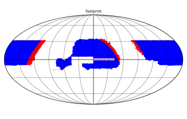
Figure 1: The footprints of the DECaLS galaxies of LS DR9 used for weak lensing reconstruction (blue) and the DECaLS galaxies of LS DR8 with shear measurement (red). The two catalogs have a footprint overlap of $8365\deg^{2}$.

Sample	Magnitude Range	Galaxy Number	$\bar{n}({\rm arcmin}^{-2})$	$a$	$g$	$w$	band
1	(22.8, 23.0)	5590717	0.19	0.51	-0.99	-0.09	g
2	(22.6, 22.8)	5590717	0.19	1.20	0.40	-0.00	g
3	(22.3, 22.6)	5590717	0.19	1.83	1.65	0.09	g
4	( , 22.3)	5590717	0.19	2.57	3.14	0.20	g
5	(22.0, 22.2)	7740929	0.26	0.94	-0.12	0.04	r
6	(21.7, 22.0)	7740929	0.26	1.10	0.20	0.07	r
7	(21.4, 21.7)	7740929	0.26	1.47	0.94	0.06	r
8	( , 21.4)	7740929	0.26	2.11	2.22	0.03	r
9	(21.3, 21.6)	9882012	0.33	0.64	-0.72	-0.08	z
10	(21.0, 21.3)	9882012	0.33	0.65	-0.70	-0.11	z
11	(20.5, 21.0)	9882012	0.33	1.01	0.02	-0.11	z
12	( , 20.5)	9882012	0.33	1.76	1.51	-0.09	z

Table 1: Summary of the galaxy sub-samples used for lensing reconstruction. We use galaxies in the photo-z range $0.5<z_{\kappa}<0.8$. Throughout the paper we use $z_{\kappa}$ to denote the (photometric) redshift of galaxies used for lensing reconstruction, and use $z_{\gamma}$ for redshift of galaxies for cosmic shear measurements. In addition to the information presented in the table, it should be noted that there are overlaps between the sub-samples in terms of the galaxies they contain. For example, sample 1 and sample 5 share a common set of $1.7\times 10^{6}$ galaxies, which we denote as $n_{15}=5.4\times 10^{6}$. Similarly $n_{16}=1.4\times 10^{6}$ and $n_{17}=0.7\times 10^{6}$. However $n_{ij}=0$ if sample i and j are from the same photometry band (e.g. $n_{12}=n_{13}=0$).

Figure 2: The maps showing the galaxy number overdensity defined by Eq.(18), for the 12 flux bins. The HEALPix resolution parameter $N_{\rm side}=256$. The columns from left to right represent the $g$, $r$, and $z$ bands, respectively. The rows increase in flux from top to bottom.

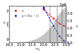
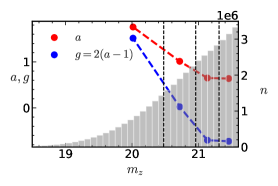
Figure 3: The results of $a$ and $g$ factors for each flux bin, and histogram plot of the galaxy number counts as a function of magnitude in the three bands. The vertical black dashed lines mark the boundaries of the flux bin cuts. The left y-axis represents the values of $a$ and $g$ factors, while the right y-axis displays the galaxy number count.

III Data analysis

We apply our method of lensing reconstruction to the DECaLS galaxies of the DESI imaging surveys (Dey et al., 2019) Data Release 9 (LS DR9).

III.1 Data

The DECaLS data are processed by Tractor (Lang et al., 2016a; Meisner et al., 2017). The galaxy samples used for lensing reconstruction are created in accordance with the selection criteria outlined in section 2.1 of Yang et al. (2021). We summarize the main steps here. First, we select out extended imaging objects according to the morphological types provided by the TRACTOR software (Lang et al., 2016b). We choose objects that have been observed at least once in each optical band to ensure a reliable photo-$z$ estimation. We also remove the objects within $|\mathrm{b}|<25.0^{\circ}$ (where $\mathrm{b}$ is the Galactic latitude) to avoid high stellar density regions. Finally, we remove any objects whose fluxes are affected by the bright stars, large galaxies, or globular clusters (maskbits 1,5,6,7,8,9,11,12,13 ). The sky coverage of our selected DECaLS sample is shown in Fig.1. We apply identical selections to the publicly available random catalogues .

For the convergence-shear cross-correlation analysis, we utilize the shear measurements from DECaLS galaxies of DESI imaging surveys DR8 (LS DR8), with a sky coverage of $8960\deg^{2}$. The footprint of the DECaLS galaxies of LS DR8 is shown in Fig.1. These galaxies are then divided into five types according to their morphologies: PSF, SIMP, DEV, EXP, and COMP. The ellipticity $e_{1,2}$ are estimated – except for the PSF type – by a joint fit on the three optical $g$-, $r$-, and $z$-band. The potential measurement bias are modeled with (Hildebrandt et al., 2012; Miller et al., 2013; Hildebrandt et al., 2017),

$$\gamma^{\mathrm{obs}}=(1+m)\gamma^{\text{true }}+c\ .$$

The additive bias $c$ and the multiplicative bias $m$ is expected to come from residuals in the anisotropic PSF correction, measurement method, blending and crowding (Mandelbaum et al., 2015; Euclid Collaboration et al., 2019). This calibration is obtained by comparing with Canada–France–Hawaii Telescope (CFHT) Stripe 82 observed galaxies and Obiwan simulated galaxies (Phriksee et al., 2020; Kong et al., 2020). For both DECaLS galaxies of LS DR8 and DR9 , we employ the photometric redshift based on Zhou et al. (2021), which is estimated using the $g,r$, and $z$ optical bands from DECaLS and $W1$ and $W2$ infrared bands from WISE (Wide-field Infrared Survey Explorer, Wright et al. 2010).

III.2 Reconstruction

To reconstruct the convergence map we select DECaLS galaxies of LS DR9 with $0.5\leq z_{p}\leq 0.8$. Here $z_{p}$ is the best-fit value of the photometric redshift of a galaxy. For each bands we select galaxies with magnitude $m_{g}\leq 23.0,m_{r}\leq 22.2,m_{z}\leq 21.6$. Here $m_{g},m_{r},m_{z}$ are the magnitudes in $g,r,z$ band. The magnitude cut of each band is set 0.1 lower than the peak position of the galaxy number counts as a function of the magnitude (Fig.3). This serves as an approximation for the flux-limit selection. Then we equally divide galaxies of each band into $N_{F}=4$ flux bins. This yields 12 flux bins in total. We have other sets of choice of the magnitude cuts and $N_{F}$ for consistency tests, which is described in Sec IV.1. Table 1 shows a summary of these galaxy sub-samples.

For each flux bin, we project the 3D galaxy number density distribution to 2D sky map along the line-of-sight in the $N_{\rm side}$ = 512 resolution. We then downgrade the pixelized map to $N_{\rm side}$ = 256. We select areas pixels with an observed coverage fraction $f_{\beta}$ larger than a threshold $f^{\rm threshold}$, where $f_{\beta}$ is defined as

$$f_{\beta}=\frac{\sum\limits_{i=1}^{16}\mathcal{M}_{i}}{\sum\limits_{i}}\ .$$ (17)

Here $\mathcal{M}_{i}$ is the survey mask in $N_{\rm side}=512$ map, which is created from the random catalogs by selecting random point with exposure time in all three bands greater than zero. This step is to minimize the impact from the footprint-induced fake clustering. For $f_{\beta}\geq f^{\rm threshold}$, we assign to each pixel $\beta$ its coverage fraction $f_{\beta}$. We use this value as a weight in the clustering measurements. We consider three choices of $f^{\rm threshold}$ later for consistency tests but fiducial one is 0.9. After this selection, we get the galaxy overdensity for the 12 flux bins,

$$\hat{\delta}^{\beta}_{i}=\frac{N^{\beta}_{i}/f^{\beta}}{\langle N^{\beta}_{i}/f^{\beta}\rangle}-1\ .$$ (18)

Here $N_{i}^{\beta}$ is the galaxy number count of $i$-th flux bin in the $\beta$-th pixel. The average $\langle\cdots\rangle$ is over all pixels with $f\geq f^{\rm threshold}$. Fig.2 shows the obtained galaxy overdensity maps.

We then apply the $\kappa$ estimator described in Section II to the galaxy overdeisity maps. Fig.3 shows the galaxy number count as a function of magnitude and the estimated $a$ and $g$ factors for each magnitude bin. The numerical calculation of $a$ of the flux bin $F\in[f_{1},f_{2}]$ is conducted by

$$a= \frac{\log\left(\int_{f_{1}/(1+2\delta_{F})}^{f_{2}/(1+2\delta_{F})}n(F)dF\right)-\log\left(\int_{f_{1}(1+2\delta_{F})}^{f_{2}(1+2\delta_{F})}n(F)dF\right)}{2\log(1+2\delta_{F})}$$ (19)

We find that the numerical calculation converges for $|\delta_{F}|<0.1$ and we take the result from $\delta_{F}=0.02$.

The results of the $N_{ij}\equiv\frac{\bar{n}_{ij}}{\bar{n}_{i}\bar{n}_{j}}$ are shown in Fig.4. Applying Eq.(8) yields the $w_{i}$’s for each flux bin, which is shown in Fig.5. We then get the reconstructed convergence map sampled on HEALPix pixels by a weighted sum over the galaxy overdensity maps (Eq.(4)). We select pixels with $f\geq f^{\rm threshold}$ for the cross correlation measurement.

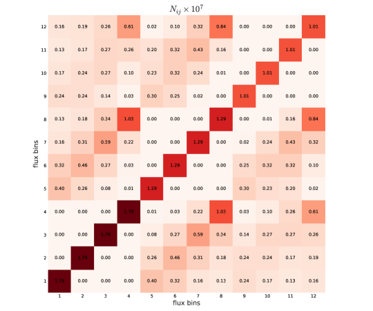
Figure 4: The normalized galaxy surface number density matrix $N_{ij}\equiv\frac{\bar{n}_{ij}}{\bar{n}_{i}\bar{n}_{j}}$. The diagonal elements $N_{ii}\equiv\frac{1}{\bar{n}_{i}}$ are the normalized galaxy surface number density of each flux bin. The off-diagonal elements $N_{ij}$ are that between the $i$-th and $j$-th flux bin.

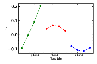
Figure 5: The results of the weights calculated by Eq.(8) for each flux bin. The estimator for the lensing convergence is obtained by calculating the weighted average of the galaxy number overdensity.

III.3 Imaging systematics

Observation conditions, such as stellar contamination, Galactic extinction, sky brightness, seeing, and airmass, introduce spurious fluctuations in the observed galaxy density. Therefore, our reconstruction method based on galaxy density are potentially biased. In this work, we apply the Random Forest (RF) technique (a the machine learning based regression approach, Chaussidon et al., 2021) to mitigate the imaging systematics, following the precedure described in Xu et al. (2023). Applying the RF, a weight factor $w_{\mathrm{pix},i}$ for each valid pixel $i$ will be returned. The imaging systematics will be reduced by weighting the reconstructed convergence map $\kappa_{\text{GRID }}$ according to their pixel weights.

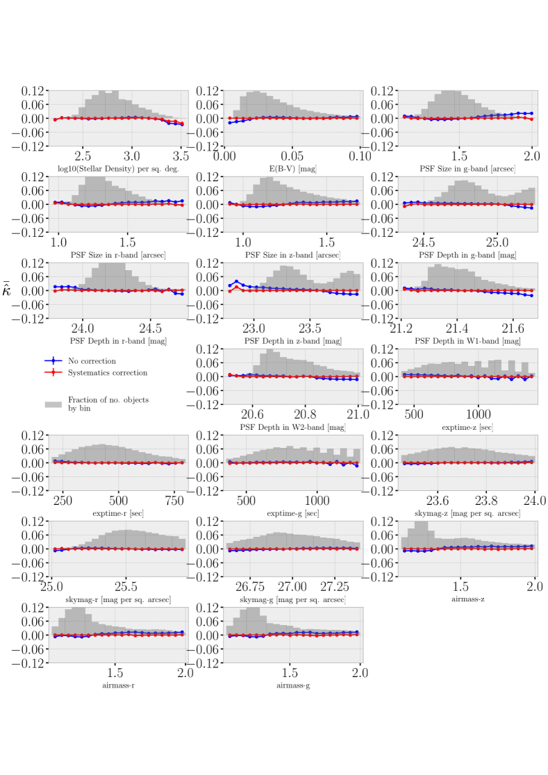
Figure 6: Average value of the reconstructed convergence field as a function of 19 input imaging maps. The blue/red lines show the relative density before/after the systematics correction. The histogram is the fraction of pixels in bins of imaging properties, which is used to estimate the errors as the standard deviation of the convergence field in bins. After mitigating the imaging systematics, the convergence field show little fluctuation with respective to imaging properties.

Fig.6 shows the distribution of the reconstructed convergence field, before and after the mitigation, as a function of 19 input imaging properties. If the convergence field is independent of imaging properties, one would expect the mean value of $\hat{\kappa}$ in bins of imaging properties amounts to the global mean. We can see that the reconstructed field suffers some imaging contamination at percent level. After the mitigation, the corrected density is almost flat for all imaging properties. Mitigating the imaging systematics enhances the detection significance of the weak lensing signal, which will be presented in Section IV. After mitigating the imaging systematics, we get the final convergence map $\kappa_{\text{GRID }}$. Fig.7 shows the reconstructed convergence map before and after the imaging systematics mitigation. The Weiner filtered convergence map is also presented in Fig.7. The details of the Weiner filtering procedure are presented in the Appendix.

Figure 7: The reconstructed lensing convergence map $\kappa_{\text{GRID }}$ sampled on HEALPix pixels with $N_{\rm side}$ = 256. The left panel shows the map before the imaging systematics mitigation, and the middle panel shows the map after the mitigation. The right panel shows the map after the mitigation and the application of the Wiener filter. The lower panels correspond to zoomed-in views of the areas indicated by the red box in the upper panels.

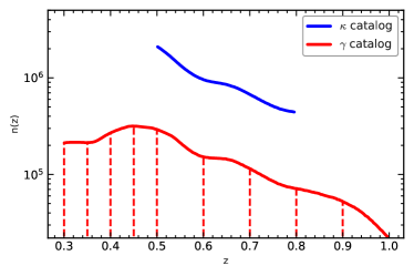
Figure 8: The photometric redshift distributions of the DR9 galaxies used for lensing construction (blue line) and the DR8 galaxies with shear measurement (red line). The vertical dashed lines represent the boundaries of the photo-z bins for the shear catalog, defined for cross correlation analysis.

III.4 Cross correlation measurement

To access the quality of the reconstructed map, we measure its cross-correlation with the DECaLS cosmic shear catalogs of LS DR8. The two catalogs have an overlap in their footprints (Fig. 1) of approximately $8365\deg^{2}$. We select the shear galaxies with $0.3<z_{\rm p}<1.0$, which yields $\sim$35 million galaxy shear samples. The shear galaxies are then divided into nine photo-$z$ bins with edges at 0.3, 0.35, 0.4, 0.45, 0.5, 0.6, 0.7, 0.8, 0.9 and 1.0. For each photo-$z$ bin, we estimate the convergence-shear cross-correlation function by

$$\hat{\xi}^{\kappa\gamma}(\theta)=\langle\kappa_{\text{GRID }}\gamma_{t}\rangle_{\theta}/(1+\bar{m})\ .$$ (20)

Here the average $\langle\cdots\rangle_{\theta}$ is over all pixel-galaxy pairs within angular separation $\theta$, and $\bar{m}$ is the average shear multiplicative bias. The calculations are done using the public available code TreeCorr. We use $N=100$ Jackknife patches to estimate the covariance matrix

$$\textbf{Cov}_{\alpha\beta}=\frac{N-1}{N}\sum\limits_{n=1}^{N=100}[(\hat{\xi}^{\kappa\gamma}_{n}(\theta_{\alpha})-\overline{\xi}^{\kappa\gamma}(\theta_{\alpha}))\times(\hat{\xi}^{\kappa\gamma}_{n}(\theta_{\beta})-\overline{\xi}^{\kappa\gamma}(\theta_{\beta}))]\ .$$ (21)

Here $\overline{\xi}^{\kappa\gamma}$ is the average over the 100 patches. For each photo-z bin, the data vector size is 6, and we rescale the covariance matrix following Percival et al. (2014); Wang et al. (2020) to get an unbiased estimation.

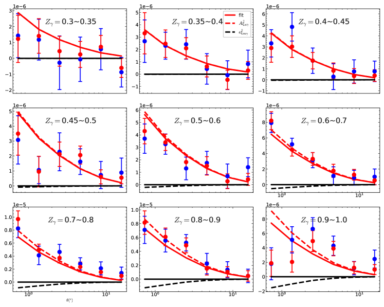
Figure 9: Measured cross correlation function between the reconstructed convergence and the shear. The red/blue data points denotes the results with/without imaging systematics mitigation. The solid lines represent the best-fit, where the fitted values of $A$ and $\epsilon$ are the same for each shear bin. The dashed lines denote the two components of the best-fit model. For clarity we only show the best-fit for the measurements after the mitigation. The comparison of the fitting before and after the mitigation is summarized in Table 3.

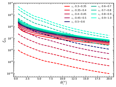
Figure 10: The theoretical cross correlation templates, under the Planck 2018 cosmology. Different colors are used to distinguish the results of different photo-$z$ bins of the shear. The signal term $\xi^{\kappa\gamma}$ is represented by the solid lines, while the contamination term $\xi^{\kappa m}$ is denoted by the dashed lines.

For the theoretical calculation of $\xi^{\kappa\gamma}(\theta)$ and $\xi^{m\gamma}(\theta)$, we apply the Core Cosmology Library (CCL, Chisari et al. 2019) and use HaloFit (Smith et al., 2003; Takahashi et al., 2012; Mead et al., 2015) to calculate the nonlinear matter power spectrum. The galaxy redshift distribution $n(z)$ are calculated for each tomographic bin, combining the photo-$z$ distribution and a Gaussian photo-$z$ error PDF with $\sigma_{z}=0.05$. Fig.8 displays the photo-$z$ distribution of the DR9 galaxies used for lensing construction and the DR8 shear catalog. The theoretical results of $\xi^{\kappa\gamma}(\theta)$ and $\xi^{m\gamma}(\theta)$ are shown in Fig.10. The difference in their shape and redshift dependence allow us to distinguish between the two terms.

IV Results

The results of the cross correlation are show in Fig.9. Significant cross-correlation signals are obtained. We fit the measured cross correlation against the theoretical model (Eq.(12)) and constrain the two free parameters. The constraints on $A$ can reveal the potential biases in the lensing reconstruction or in the cross correlation analysis, if its deviation from one is observed. The constraints on $\epsilon$ indicate the level of systematic errors. The $\chi^{2}$ for the fitting can be approximated by

$$\chi^{2}\approx\sum\limits_{j\alpha\beta}\big{[}\hat{\xi}^{\kappa\gamma}_{j}(\theta_{\alpha})-{\xi}_{j,\rm th}(\theta_{\alpha})\big{]}\textbf{Cov}_{j\ \alpha\beta}^{-1}\big{[}\hat{\xi}^{\kappa\gamma}_{j}(\theta_{\beta})-{\xi}_{j,\rm th}(\theta_{\beta})\big{]}\ .$$ (22)

Here $\hat{\xi}^{\kappa\gamma}_{j}$ and ${\xi}_{j,\rm th}$ denote the measurement and the model in the $j$-th photo-$z$ bin of shear, respectively. Cov is the data covariance matrix. $A$ and $\epsilon$ are identical for each photo-$z$ bin and so the sum is over all the data points and photo-$z$ bins.

The best fit is

$$\big{(}A^{\text{bestfit}}\ \epsilon^{\text{bestfit}}\big{)}^{\mathbf{T}}=\bm{F}^{-1}\bigg{[}\sum_{j}\bm{\xi}_{j}^{\mathbf{T}}\textbf{Cov}_{j}^{-1}\bm{\hat{\xi}}_{j}\bigg{]}\ ,$$ (23)

where

$$\bm{\xi}_{j}\equiv\begin{pmatrix}\xi_{j}^{\kappa\gamma}(\theta_{1})&\xi_{j}^{\kappa m}(\theta_{1})\\ \xi_{j}^{\kappa\gamma}(\theta_{2})&\xi_{j}^{\kappa m}(\theta_{2})\\ \vdots&\vdots\\ \xi_{j}^{\kappa\gamma}(\theta_{n})&\xi_{j}^{\kappa m}(\theta_{n})\end{pmatrix};\hat{\bm{\xi}}_{i}\equiv\begin{pmatrix}\hat{\xi}_{j}^{\kappa\gamma}(\theta_{1})\\ \hat{\xi}_{j}^{\kappa\gamma}(\theta_{2})\\ \vdots\\ \hat{\xi}_{j}^{\kappa\gamma}(\theta_{n})\end{pmatrix}\ .$$ (24)

The associated errors and covariance matrix of the constraints are given by $\bm{F}^{-1}$. $\bm{F}$ is the fisher matrix of $A$ and $\epsilon$,

$$\bm{F}= \begin{pmatrix}\sum\limits_{j\alpha\beta}\xi^{\kappa\gamma}_{j,\alpha}\textbf{Cov}_{j,\alpha\beta}^{-1}\xi^{\kappa\gamma}_{j,\beta}&\sum\limits_{j\alpha\beta}\xi^{\kappa\gamma}_{j,\alpha}\textbf{Cov}_{j\ \alpha\beta}^{-1}\xi^{\kappa m}_{j,\beta}\\ \sum\limits_{j\alpha\beta}\xi^{\kappa\gamma}_{j,\alpha}\textbf{Cov}_{j\ \alpha\beta}^{-1}\xi^{\kappa m}_{j,\beta}&\sum\limits_{j\alpha\beta}\xi^{\kappa m}_{j,\alpha}\textbf{Cov}_{j\ \alpha\beta}^{-1}\xi^{\kappa m}_{j,\beta}\end{pmatrix}\$$

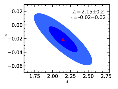
Figure 11: Contour plot of the constraints on $A$ and $\epsilon$, where the triangular point denote the best-fit value. The contour levels are 1- and 2-$\sigma$.

Fig.11 shows the results of the constraints. According to $A$, we detect a convergence-shear cross-correlation signal with $S/N\equiv A/\sigma_{A}\simeq 10$. According to $\epsilon$, the galaxy intrinsic clustering is suppressed by a factor by a factor $\sim 50$, to a level of $-0.02\pm 0.02$. The residual galaxy clustering contamination in the $\hat{\kappa}$ map is consistent with zero. The best-fit to the cross-correlation is shown in Fig.9, and the two components $A\xi^{\kappa\gamma}$ and $\epsilon\xi^{m\gamma}$ are also highlighted in the figure. The $\epsilon\xi^{m\gamma}$ term is subdominant for all cases.

Unfortunately, a significant deviation from one is detected in $A$. There are possible uncertainties that may lead to this bias, such as the $S_{8}$ tension between the low-$z$ and the CMB measurements, the photo-$z$ error, and the shear measurement error. Out of all the factors, the measurement error/bias in $g=2(a-1)$ should be the primary cause of the discrepancy of factor $\sim 2$. In this work it is determined by flux-based method, i.e. the logarithmic slope of the luminosity function (Eq.(2)). It is unbiased if the galaxy samples are strictly flux-limited. However the real galaxy samples are a complex selection of flux, color, position and shape. Consequently, biases arise in flux-based methods when estimating the magnification coefficient in real samples. Even when taking into account a simplified survey selection function, this bias may reach $\sim 2-3$ (von Wietersheim Kramsta et al., 2021; Elvin-Poole et al., 2023), comparable to the bias observed in this work. The actual magnification coefficients could be investigated by forward modeling the real selection functions (e.g., Elvin-Poole et al., 2023), which will help reduce the bias. We leave it for future studies.

Table 3 lists the results of $\chi^{2}_{\rm min}$ and ${\chi^{2}_{\rm null}}$to demonstrate the goodness of fit to the model, where the $\chi^{2}_{\rm null}$ and $\chi^{2}_{\rm min}$ is defined by

$$\chi^{2}_{\rm null}=\sum\limits_{j\alpha\beta}\big{[}\hat{\xi}^{\kappa\gamma}_{j}(\theta_{\alpha})\big{]}\textbf{Cov}_{j\ \alpha\beta}^{-1}\times\big{[}\hat{\xi}^{\kappa\gamma}_{j}(\theta_{\beta})\big{]}\ ,$$ (25)

$$\chi^{2}_{\rm min}=\sum\limits_{j\alpha\beta}\big{[}\hat{\xi}^{\kappa\gamma}_{j}(\theta_{\alpha})-{\xi}_{j,\rm th}^{\rm bestfit}(\theta_{\alpha})\big{]}\textbf{Cov}_{j\ \alpha\beta}^{-1}$$

$$\times\big{[}\hat{\xi}^{\kappa\gamma}_{j}(\theta_{\beta})-{\xi}_{j,\rm th}^{\rm bestfit}(\theta_{\alpha})\big{]}\ ,$$ (26)

where

$$\xi_{\rm th}^{\rm bestfit}=A^{\rm bestfit}\xi^{\kappa\gamma}+\epsilon^{\rm bestfit}\xi^{m\gamma}\ .$$ (27)

The degree-of-freedom (d.o.f) of the fitting is $52$ and the $\chi^{2}_{\rm min}\simeq 59$. Therefore, the two parameter fitting returns reasonable $\chi^{2}_{\rm min}$/d.o.f. $\sim 1$. This means that shape of the measured cross-correlation agrees with the model prediction, and provides support that the detected signal is cosmological in origin. With 54 non-independent data points and the full covariance, $\chi^{2}_{\rm null}=367.6$ and $\chi^{2}_{\min}=58.7$ with respect to the null and to the model, respectively. According to the data-driven signal-to-noise ratio $\sqrt{\chi^{2}_{\rm null}}$, we get $19.1\sigma$ detection of a non-zero cross-correlation signal. According to the fitting-driven signal-to-noise ratio $\sqrt{\chi^{2}_{\rm null}-\chi^{2}_{\rm min}}$, the significance is $\sim 10.7\sigma$. We compared the results before and after the imaging systematics mitigation in Table 3. It shows that the fitting results are consistent, and after the mitigation, both $\sqrt{\chi^{2}_{\rm null}-\chi^{2}_{\rm min}}$ and $A/\sigma_{A}$ exhibit an increase from 15.1 to 17.6 and 8.5 to 10.8, respectively.

IV.1 Internal test

We test the impact of several factors in the analysis, which are summarized in Table 3. First, we compare the results for $f^{\rm threshold}=0.5,0.7,0.9$. Larger $f^{\rm threshold}$ indicates more stringent selection of the pixels of galaxy number overdensity map. Table 3 shows that the impact of $f^{\rm threshold}$ is small, and the fitting result is stable for different $f^{\rm threshold}$.

Second, we test the cases of $N_{F}=2,3,4$ and find that the constraints on $A$ and $\epsilon$ are stable for different $N_{F}$. The $\epsilon=\Sigma_{i}w_{i}b_{i}$ depends on the galaxy biases in the selected flux bins and, consequently, on the number of flux bins $N_{F}$. The $\epsilon$ is consistently to be a minimal value for different $N_{F}$. It indicates that our method of eliminating the galaxy intrinsic clustering is robust.

Third, we test the influence of the magnitude cut on the results. We select galaxies which are 0.5 magnitude brighter than the baseline set. The first case involves selecting galaxies that are 0.5 magnitudes brighter across all three bands, denoted as $m_{g,r,z}-0.5$. The other three cases involve selecting galaxies that are 0.5 magnitudes brighter in each band individually, denoted as $m_{g}-0.5$, $m_{r}-0.5$ and $m_{z}-0.5$. As shown in Table 3, $\epsilon$ remains minimal for all the cases. However the results of $A$ are significantly affected by the magnitude cuts. This discrepancy observed in $A$ is reasonable. It supports our hypothesis that the error/bias in $g=2(a-1)$ is the primary contributor to the multiplicative error in the overall amplitude of $\hat{\kappa}$. A brighter magnitude cut of 0.5 results in a decrease of $\sim$ 30$-$40% in the number of galaxies for a particular photometry band. It then results in modifications to the selection functions of the galaxy samples, thereby inducing alterations in the magnification coefficient. The level of the bias can extend up to a factor of 3 for the $m_{r,g,z}-0.5$ case, which is unlikely to result from other systematics. The impact of magnitude cuts on the magnification coefficient is also investigated in von Wietersheim Kramsta et al. (2021). Their results support our findings, showing that modification in the magnitude cut can lead to the magnification coefficient ranging from 1.5 to 3.0.

In addition, Table 3 presents the comparison of fitting results before and after mitigating the imaging systematics for all the tests investigated above. Across all cases, the fitting results are consistent and exhibit enhancements in the S/N after the mitigation, indicating the effectiveness and robustness of the mitigation procedure.

IV.2 Model selection

	baseline	A=0	A=1	$\epsilon$=0
$\chi^{2}_{\rm min}$	58.7	169.2	90.3	59.9
AIC	62.8	171.3	92.3	62.0

Table 2: $\chi^{2}_{\rm min}$ and AIC scores for the baseline and the three alternative models.

Performing an Akaike information criterion (AIC) analysis can provide valuable insights into which model is the most suitable for explaining the observed data. In this part, we modify the theoretical template to facilitate the comparison of different models. In addition to the baseline model described by Eq. (12), we also consider alternative models which we keep either $A$ or $\epsilon$ fixed. We compare four cases: the baseline model, fixing $A=0$, fixing $A=1$, and fixing $\epsilon=0$. For each model we repeat the fitting process and then calculate the AIC, which can be expressed, to second-order, as:

$$\mathrm{AIC}_{\mathrm{c}}=-2\ln p\left(\lambda_{\text{bestfit }}\mid D\right)+2N_{\lambda}+\frac{2N_{\lambda}+1}{N_{D}-N_{\lambda}-1}.$$

Here $N_{\lambda}$ is the number of parameters, $N_{D}$ is the number of data points, $p$ is the likelihood which is Gaussian in our case and $p\left(\lambda_{\text{bestfit }}\mid D\right)$ is the value for the best-fit parameters. The ”best” model has the smallest AIC. If another model’s AIC is larger by 10 or more, this model should be ruled out. If the difference is less than 2, the two models can not be really distinguished.

Table 2 shows the results of $\chi^{2}_{\rm min}$ (the minimum $\chi^{2}$ value obtained during fitting) and AIC. The model that fixes $\epsilon=0$ has the lowest AIC score and is 0.8 lower than that of the baseline model. It reinforces the conclusion that the residual galaxy clustering contamination in the $\hat{\kappa}$ map is insignificant. The model that fixes $A=0$ has an AIC score that is roughly 108 higher than the baseline, ruling out null detection of weak lensing signal. The model that fixes $A=1$ displays an AIC score $\sim$30.0 higher than the baseline. This implies the significance of the multiplicative error in the overall amplitude of $\hat{\kappa}$, which we attribute to the limitation of the flux-based method in accurately estimating the magnification coefficient.

IV.3 Impact of the galaxy intrinsic clustering

To eliminate the average galaxy clustering in the lensing reconstruction, we initially employed the condition $\sum w_{i}=0$. However, we can reevaluate the impact of average galaxy clustering by modifying the condition to

$$\sum_{i}w_{i}\hat{b}_{i}=0\ .$$ (28)

Here, the values of $\hat{b}_{i}$ are artificially selected. Setting all $\hat{b}_{i}$’s equal to a constant reduces to the original condition. Selecting forms that $\hat{b}_{i}$’s deviate from a constant will enhance the impact of the galaxy clustering. The results of $\epsilon$ are expected to be dependent on the form of $\hat{b}_{i}$’s, while those of $A$ are not. We use a simple form of $\hat{b}_{i}$ as a demonstration. For each band, we set $\hat{b}_{i}$ for the four flux bins to be

$$1-2\Delta\hat{b},1-\Delta\hat{b},1+\Delta\hat{b},1+2\Delta\hat{b}$$ (29)

The only parameter is $\Delta\hat{b}$, which we set to be identical for each band. We sample $\Delta\hat{b}$ in the range $[-0.25,0.25]$ with bin width $0.05$. For each $\Delta\hat{b}$ we repeat the lensing reconstruction procedure and conduct the cross-correlation analysis to obtain the constraints on $A$ and $\epsilon$.

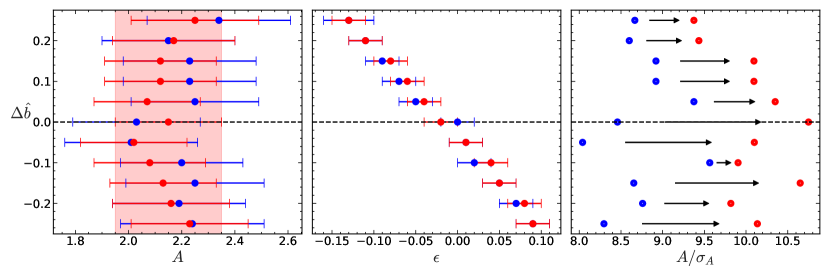
Figure 12: Impact of varying the condition $\sum w_{i}\hat{b}_{i}$ on the constraints of $A$ (the left panel), $\epsilon$ (the middle panel) and $A/\sigma_{A}$ (the right panel). The red/blue data points denotes the results with/without imaging systematics mitigation. In the left panel, the shaded regions represent the $1\sigma$ error in the constraint on $A$ for the baseline configuration, which corresponds to $\Delta\hat{b}=0$ and includes imaging systematics mitigation.

Fig.12 shows the impact of $\Delta\hat{b}$ on the results of constraints. The best fit of $A$ is insensitive to the choice of $\Delta\hat{b}$, as expected, showing the stability of the reconstruction. However, the results of $\epsilon$ exhibit significant dependence on $\Delta\hat{b}$, and tend to have a linear relation with $\Delta\hat{b}$. Its deviation from zero is significant when $|\Delta\hat{b}|$ differs considerably from zero. Therefore by varying the condition to Eq. (28), we revealed the evidence of galaxy clustering which contaminates the cosmic magnification. The initial condition for the baseline (i.e. $\Delta\hat{b}=0$ s.t. $\sum w_{i}=0$) is almost optimal in terms of reducing this contamination. Because $\epsilon$ fluctuates around zero when $\Delta\hat{b}$ is near zero and the S/N $\equiv A/\sigma_{A}$ reaches maximum when $\Delta\hat{b}=0$ (the right panel in Fig.12).

The above results imply that the galaxy deterministic biases exhibit minimal dependence on the magnitude, such that $\sum w_{i}\sim 0$. It agrees with recent findings with hydrodynamic simulations, including one based on TNG (Nelson et al., 2018; Springel et al., 2018) by Zhou et al. (2023) and another using CosmoDC2 (Korytov et al., 2019) by our companion work (Ma et al., 2023). Fig.12 also shows that the imaging mitigation enhances S/N for all the investigated cases of $\Delta\hat{b}$.

	$\quad A$	$\quad\epsilon$	$\chi^{2}_{\rm min}$	$\chi^{2}_{\rm null}$	$\sqrt{\chi^{2}_{\rm null}-\chi^{2}_{\rm min}}$	$A/\sigma_{A}$
baseline	2.15$\pm$0.20(2.03$\pm$0.24)	-0.02$\pm$0.02(-0.00$\pm$0.02)	58.7(59.2)	367.6(286.7)	17.6(15.1)	10.8(8.5)
f=0.5	2.00$\pm$0.20(2.16$\pm$0.23)	-0.00$\pm$0.02(-0.02$\pm$0.02)	55.0(56.9)	393.2(313.7)	18.4(16.0)	10.0(9.4)
f=0.7	2.10$\pm$0.20(2.11$\pm$0.25)	-0.01$\pm$0.02(-0.02$\pm$0.02)	53.0(61.2)	404.5(266.8)	18.8(14.3)	10.5(8.4)
$N_{F}=2$	2.14$\pm$0.21(2.21$\pm$0.24)	-0.01$\pm$0.02(-0.01$\pm$0.02)	58.5(63.8)	389.4(322.8)	18.2(16.1)	10.2(9.2)
$N_{F}=3$	1.79$\pm$0.20(1.85$\pm$0.23)	0.02$\pm$0.02(0.01$\pm$0.02)	55.9(61.0)	363.9(307.8)	17.6(15.7)	8.9(8.0)
$m_{g,r,z}-0.5$	3.09$\pm$0.30(2.97$\pm$0.36)	-0.08$\pm$0.03(-0.06$\pm$0.03)	41.1(43.2)	242.3(208.3)	14.2(12.8)	10.3(8.2)
$m_{g}-0.5$	2.09$\pm$0.25(2.09$\pm$0.33)	-0.00$\pm$0.02(-0.00$\pm$0.03)	47.5(41.8)	248.2(172.4)	14.2(11.4)	8.4(6.3)
$m_{r}-0.5$	1.24$\pm$0.19(1.45$\pm$0.23)	0.06$\pm$0.02(0.05$\pm$0.02)	63.5(63.1)	348.2(277.6)	16.9(14.7)	6.5(6.3)
$m_{z}-0.5$	2.13$\pm$0.20(2.24$\pm$0.25)	-0.04$\pm$0.02(-0.05$\pm$0.02)	48.0(48.2)	288.3(221.9)	15.5(13.2)	10.7(9.0)

Table 3: The impact of $f^{\rm threshold},N_{\rm F}$, the three bands magnitude cuts and the imaging systematics mitigation on the analysis. The fiducial sets are $f^{\rm threshold}=0.9,N_{\rm F}=4,m_{g}=23.0,m_{r}=22.2,m_{z}=21.6$. The d.o.f. = 52. The main table shows the results after the mitigation, while in parentheses are the results before the mitigation.

IV.4 Impact of the shear redshifts

The parameters $A$ and $\epsilon$ characterize the reconstructed lensing convergence and are therefore independent of the shear catalog utilized. Consequently, the constraints on $A$ and $\epsilon$ are expected to remain consistent when different shear catalogs are employed for cross-correlation analysis. In this part, we investigate the impact of selecting different redshift bins for the shear by systematically excluding one shear redshift bin at a time. We then perform cross-correlation analysis and constrain $A$ and $\epsilon$ using the remaining redshift bins. The results of this test are presented in Fig. 13. For all cases except the redshift bin $[0.9-1.0]$, the constraints on $A$ and $\epsilon$ align with the baseline set within the $1\sigma$ error range. The discrepancy observed in the redshift $[0.9-1.0]$ can be attributed to the lower galaxy number density (Fig.8) and consequently, a less accurate detection of the correlation function (Fig.10).

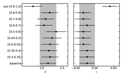
Figure 13: Impact of the shear redshifts on the constraints of $A$ (the left panel) and $\epsilon$ (the right panel). We drop one shear redshift bin at a time, and perform the cross correlation analysis and constrain the parameters with the remaining bins. The y-axis denote the shear redshift bin that is dropped. The shadow regions shows the $1\sigma$ error of the constraints for the baseline set (i.e., all the bins are included).

V SUMMARY and discussion

Based on cosmic magnification, we reconstruct weak lensing convergence map from the DECaLS DR9 galaxy catalog. Notably, this represents the first instance of a directly measured lensing map from magnification, covering a quarter of the sky. It is done by weighing overdensity maps of galaxies in different magnitude bins and different photometry bands. To test validity of the reconstruction, we make cross correlation to the galaxy shear measurement and compare to the theoretical model. We find that the galaxy intrinsic clustering is well eliminated by our method and we get $\sim 10\sigma$ detection of the convergence-shear cross correlation.

A discrepancy in the lensing amplitude of factor $\sim 2$ is found. The most likely cause for this discrepancy is the inaccuracies in measuring the magnification coefficient, which is estimated using the logarithmic slope of the luminosity function. However, to confirm this speculation, we need to perform forward modeling of the DR9 galaxy selection function and correct the estimation of the magnification coefficient. This is our next step in the research project. Our primary focus is on the cross-correlation analysis since the auto-correlation of the reconstructed convergence map is significantly affected by the weighted shot noise (Ma et al., 2023). Existing data such as DES (Dark Energy Survey Collaboration et al., 2016) and HSC (Aihara et al., 2018) have greater survey depth and higher galaxy number than DECaLS. We plan to analyze these data to improve the magnification based lensing reconstruction. It will enable us to thoroughly account for the model’s cosmology dependence, more realistic modeling of the photo-$z$ distribution, the intrinsic alignment of galaxies, and potential contamination from the extragalactic dust.

VI APPENDIX

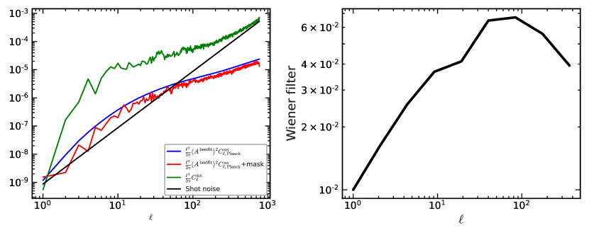
Figure 14: Left: The angular power spectrum of the weak lensing map. The blue line is calculated from the Planck 2018 cosmology combined with the bestfit lensing amplitude $A^{\rm bestfit}$, while after applying the DECaLS mask the calculation is shown with the red line. The green line is the measurement from the reconstructed convergence map. The black line represents the shot noise. Right: The associated Weiner filter calculated from the angular power spectrum.

VI.1 Weiner filter

For the spherical harmonic coefficients $\hat{\kappa}_{\ell m}$ estimated by Healpix, the Weiner filter is calculated by

$$\hat{\kappa}^{\rm WF}_{\ell m}=\frac{C_{\ell}^{\rm signal}}{C_{\ell}^{\rm signal}+C_{\ell}^{\rm noise}}\hat{\kappa}_{\ell m}\ .$$ (30)

Where $C_{\ell}^{\rm signal}$ is the auto power spectrum of the lensing signal and $C_{\ell}^{\rm noise}$ is that of the noise. We calculate $C_{\ell}^{\rm signal}$ from the Planck 2018 cosmology combined with the bestfit amplitude $A^{\rm bestfit}$. To take into account the impact of survey geometry, we generate 100 full-sky maps of the power spectrum $(A^{\rm bestfit})^{2}C^{\kappa\kappa}_{\ell,\rm Planck}$. We then apply the mask to these maps and obtain 100 power spectra with the DECaLS mask. We use the average one to get $C_{\ell}^{\rm signal}$.

We calculate $C_{\ell}^{\rm signal}+C_{\ell}^{\rm noise}$ by the auto power spectrum of the reconstructed lensing map $\hat{\kappa}$, which is

$$C_{\ell}^{\hat{\kappa}\hat{\kappa}}=\frac{1}{2\ell+1}\sum\limits_{m=-\ell}^{\ell}\hat{\kappa}_{\ell m}^{*}\hat{\kappa}_{\ell m}\ .$$ (31)

Take the reconstructed lensing map of the baseline set (the first row in Table 3) as an example, the results of the power spectrum is shown in Fig.14. The auto power spectrum of the reconstructed lensing map is overwhelmed by the shot noise at $\ell>50$, which agrees with the results in Ma et al. (2023). This is the reason why we have used the cross correlation to increase the S/N. The associated Weiner filter calculated by Eq.(30) is shown in the right panel of Fig.14 and the lensing convergence map after applying the Weiner filter is shown in Fig.7.

References

- Bartelmann and Schneider (2001a) M. Bartelmann and P. Schneider, Phys. Rep. 340, 291 (2001a), eprint astro-ph/9912508.
- Kilbinger (2015a) M. Kilbinger, Reports on Progress in Physics 78, 086901 (2015a), eprint 1411.0115.
- Bartelmann and Schneider (2001b) M. Bartelmann and P. Schneider, Phys. Rep. 340, 291 (2001b), eprint astro-ph/9912508.
- Hoekstra and Jain (2008) H. Hoekstra and B. Jain, Annual Review of Nuclear and Particle Science 58, 99 (2008), eprint 0805.0139.
- Van Waerbeke et al. (2010) L. Van Waerbeke, H. Hildebrandt, J. Ford, and M. Milkeraitis, ApJ 723, L13 (2010), eprint 1004.3793.
- Fu and Fan (2014) L.-P. Fu and Z.-H. Fan, Research in Astronomy and Astrophysics 14, 1061-1120 (2014).
- Kilbinger (2015b) M. Kilbinger, Reports on Progress in Physics 78, 086901 (2015b), eprint 1411.0115.
- Dark Energy Survey Collaboration et al. (2016) Dark Energy Survey Collaboration, T. Abbott, F. B. Abdalla, J. Aleksić, S. Allam, A. Amara, D. Bacon, E. Balbinot, M. Banerji, K. Bechtol, et al., MNRAS 460, 1270 (2016), eprint 1601.00329.
- de Jong et al. (2013) J. T. A. de Jong, G. A. Verdoes Kleijn, K. H. Kuijken, and E. A. Valentijn, Experimental Astronomy 35, 25 (2013), eprint 1206.1254.
- Aihara et al. (2018) H. Aihara, N. Arimoto, R. Armstrong, S. Arnouts, N. A. Bahcall, S. Bickerton, J. Bosch, K. Bundy, P. L. Capak, J. H. H. Chan, et al., PASJ 70, S4 (2018), eprint 1704.05858.
- Hamana et al. (2020) T. Hamana, M. Shirasaki, S. Miyazaki, C. Hikage, M. Oguri, S. More, R. Armstrong, A. Leauthaud, R. Mandelbaum, H. Miyatake, et al., PASJ 72, 16 (2020), eprint 1906.06041.
- Asgari et al. (2021) M. Asgari, C.-A. Lin, B. Joachimi, B. Giblin, C. Heymans, H. Hildebrandt, A. Kannawadi, B. Stölzner, T. Tröster, J. L. van den Busch, et al., A&A 645, A104 (2021), eprint 2007.15633.
- Giblin et al. (2021) B. Giblin, C. Heymans, M. Asgari, H. Hildebrandt, H. Hoekstra, B. Joachimi, A. Kannawadi, K. Kuijken, C.-A. Lin, L. Miller, et al., A&A 645, A105 (2021), eprint 2007.01845.
- Loureiro et al. (2022) A. Loureiro, L. Whittaker, A. Spurio Mancini, B. Joachimi, A. Cuceu, M. Asgari, B. Stölzner, T. Tröster, A. H. Wright, M. Bilicki, et al., A&A 665, A56 (2022), eprint 2110.06947.
- Amon et al. (2022) A. Amon, D. Gruen, M. A. Troxel, N. MacCrann, S. Dodelson, A. Choi, C. Doux, L. F. Secco, S. Samuroff, E. Krause, et al. (DES Collaboration), Phys. Rev. D 105, 023514 (2022), URL https://link.aps.org/doi/10.1103/PhysRevD.105.023514.
- Secco et al. (2022) L. F. Secco, S. Samuroff, E. Krause, B. Jain, J. Blazek, M. Raveri, A. Campos, A. Amon, A. Chen, C. Doux, et al. (DES Collaboration), Phys. Rev. D 105, 023515 (2022), URL https://link.aps.org/doi/10.1103/PhysRevD.105.023515.
- Li et al. (2023) X. Li, T. Zhang, S. Sugiyama, R. Dalal, M. M. Rau, R. Mandelbaum, M. Takada, S. More, M. A. Strauss, H. Miyatake, et al., arXiv e-prints arXiv:2304.00702 (2023), eprint 2304.00702.
- Blandford and Narayan (1992) R. D. Blandford and R. Narayan, ARA&A 30, 311 (1992).
- Bartelmann and Narayan (1995) M. Bartelmann and R. Narayan, in Dark Matter, edited by S. S. Holt and C. L. Bennett (1995), vol. 336 of American Institute of Physics Conference Series, pp. 307–319, eprint astro-ph/9411033.
- Bauer et al. (2014) A. H. Bauer, E. Gaztañaga, P. Martí, and R. Miquel, Monthly Notices of the Royal Astronomical Society 440, 3701 (2014), https://academic.oup.com/mnras/article-pdf/440/4/3701/3913172/stu530.pdf, URL https://app.dimensions.ai/details/publication/pub.1059915677.
- Bellagamba et al. (2019) F. Bellagamba, M. Sereno, M. Roncarelli, M. Maturi, M. Radovich, S. Bardelli, E. Puddu, L. Moscardini, F. Getman, H. Hildebrandt, et al., MNRAS 484, 1598 (2019), eprint 1810.02827.
- Chiu et al. (2016) I. Chiu, J. P. Dietrich, J. Mohr, D. E. Applegate, B. A. Benson, L. E. Bleem, M. B. Bayliss, S. Bocquet, J. E. Carlstrom, R. Capasso, et al., MNRAS 457, 3050 (2016), eprint 1510.01745.
- Chiu et al. (2020) I. N. Chiu, K. Umetsu, R. Murata, E. Medezinski, and M. Oguri, MNRAS 495, 428 (2020), eprint 1909.02042.
- Scranton et al. (2005) R. Scranton, B. Ménard, G. T. Richards, R. C. Nichol, A. D. Myers, B. Jain, A. Gray, M. Bartelmann, R. J. Brunner, A. J. Connolly, et al., ApJ 633, 589 (2005), eprint astro-ph/0504510.
- Bauer et al. (2012) A. H. Bauer, C. Baltay, N. Ellman, J. Jerke, D. Rabinowitz, and R. Scalzo, ApJ 749, 56 (2012), eprint 1202.1371.
- Morrison et al. (2012) C. B. Morrison, R. Scranton, B. Ménard, S. J. Schmidt, J. A. Tyson, R. Ryan, A. Choi, and D. M. Wittman, MNRAS 426, 2489 (2012), eprint 1204.2830.
- Tudorica et al. (2017) A. Tudorica, H. Hildebrandt, M. Tewes, H. Hoekstra, C. B. Morrison, A. Muzzin, G. Wilson, H. K. C. Yee, C. Lidman, A. Hicks, et al., A&A 608, A141 (2017), eprint 1710.06431.
- Bonavera et al. (2021) L. Bonavera, M. M. Cueli, J. González-Nuevo, T. Ronconi, M. Migliaccio, A. Lapi, J. M. Casas, and D. Crespo, A&A 656, A99 (2021), eprint 2109.12413.
- Crespo et al. (2022) D. Crespo, J. González-Nuevo, L. Bonavera, M. M. Cueli, J. M. Casas, and E. Goitia, A&A 667, A146 (2022), eprint 2210.17318.
- Ménard et al. (2010) B. Ménard, R. Scranton, M. Fukugita, and G. Richards, MNRAS 405, 1025 (2010), eprint 0902.4240.
- Jain and Lima (2011) B. Jain and M. Lima, MNRAS 411, 2113 (2011), eprint 1003.6127.
- Schmidt et al. (2012) F. Schmidt, A. Leauthaud, R. Massey, J. Rhodes, M. R. George, A. M. Koekemoer, A. Finoguenov, and M. Tanaka, The Astrophysical Journal 744, L22 (2012), URL http://dx.doi.org/10.1088/2041-8205/744/2/l22.
- Huff and Graves (2014) E. M. Huff and G. J. Graves, ApJ 780, L16 (2014).
- Duncan et al. (2016) C. A. J. Duncan, C. Heymans, A. F. Heavens, and B. Joachimi, Monthly Notices of the Royal Astronomical Society 457, 764–785 (2016), URL http://dx.doi.org/10.1093/mnras/stw027.
- Garcia-Fernandez et al. (2018) M. Garcia-Fernandez, E. Sanchez, I. Sevilla-Noarbe, E. Suchyta, E. M. Huff, E. Gaztanaga, Aleksić, J. , R. Ponce, F. J. Castander, et al., MNRAS 476, 1071 (2018).
- Liu et al. (2021) X. Liu, D. Liu, Z. Gao, C. Wei, G. Li, L. Fu, T. Futamase, and Z. Fan, Phys. Rev. D 103, 123504 (2021), eprint 2104.13595.
- Yao et al. (2023) J. Yao, H. Shan, P. Zhang, E. Jullo, J.-P. Kneib, Y. Yu, Y. Zu, D. Brooks, A. de la Macorra, P. Doel, et al., MNRAS 524, 6071 (2023), eprint 2301.13434.
- Zhang and Pen (2005) P. Zhang and U.-L. Pen, Phys. Rev. Lett. 95, 241302 (2005), eprint astro-ph/0506740.
- Yang and Zhang (2011) X. Yang and P. Zhang, MNRAS 415, 3485 (2011), eprint 1105.2385.
- Zhang et al. (2019) P. Zhang, J. Zhang, and L. Zhang, MNRAS 484, 1616 (2019).
- Yang et al. (2015) X. Yang, P. Zhang, J. Zhang, and Y. Yu, MNRAS 447, 345 (2015).
- Yang et al. (2017) X. Yang, J. Zhang, Y. Yu, and P. Zhang, ApJ 845, 174 (2017), eprint 1703.01575.
- Zhang et al. (2018) P. Zhang, X. Yang, J. Zhang, and Y. Yu, ApJ 864, 10 (2018), eprint 1807.00443.
- Hou et al. (2021) S.-T. Hou, Y. Yu, and P.-J. Zhang, Research in Astronomy and Astrophysics 21, 247 (2021), eprint 2106.09970.
- Bonoli and Pen (2009) S. Bonoli and U. L. Pen, MNRAS 396, 1610 (2009), eprint 0810.0273.
- Hamaus et al. (2010) N. Hamaus, U. Seljak, V. Desjacques, R. E. Smith, and T. Baldauf, Phys. Rev. D 82, 043515 (2010), eprint 1004.5377.
- Baldauf et al. (2010) T. Baldauf, R. E. Smith, U. Seljak, and R. Mandelbaum, Phys. Rev. D 81, 063531 (2010), eprint 0911.4973.
- Ma et al. (2023) R. Ma, P. Zhang, Y. Yu, and J. Qin, arXiv e-prints arXiv:2306.15177 (2023), eprint 2306.15177.
- von Wietersheim Kramsta et al. (2021) M. von Wietersheim Kramsta, B. Joachimi, J. L. van den Busch, C. Heymans, H. Hildebrandt, M. Asgari, T. Tr’oster, S. Unruh, and A. H. Wright, Monthly Notices of the Royal Astronomical Society 504, 1452–1465 (2021), URL http://dx.doi.org/10.1093/mnras/stab1000.
- Elvin-Poole et al. (2023) J. Elvin-Poole, N. MacCrann, S. Everett, J. Prat, E. S. Rykoff, J. De Vicente, B. Yanny, K. Herner, A. Ferté, E. D. Valentino, et al., Monthly Notices of the Royal Astronomical Society 523, 3649 (2023), ISSN 0035-8711, eprint https://academic.oup.com/mnras/article-pdf/523/3/3649/50596748/stad1594.pdf, URL https://doi.org/10.1093/mnras/stad1594.
- Zhou et al. (2023) S. Zhou, P. Zhang, and Z. Chen, MNRAS 523, 5789 (2023), eprint 2304.11540.
- Planck Collaboration et al. (2020) Planck Collaboration, N. Aghanim, Y. Akrami, M. Ashdown, J. Aumont, C. Baccigalupi, M. Ballardini, A. J. Banday, R. B. Barreiro, N. Bartolo, et al., A&A 641, A6 (2020), eprint 1807.06209.
- Limber (1953) D. N. Limber, ApJ 117, 134 (1953).
- Dey et al. (2019) A. Dey, D. J. Schlegel, D. Lang, R. Blum, K. Burleigh, X. Fan, J. R. Findlay, D. Finkbeiner, D. Herrera, S. Juneau, et al., The Astronomical Journal 157, 168 (2019).
- Lang et al. (2016a) D. Lang, D. W. Hogg, and D. J. Schlegel, The Astronomical Journal 151, 36 (2016a).
- Meisner et al. (2017) A. Meisner, D. Lang, and D. Schlegel, The Astronomical Journal 154, 161 (2017).
- Yang et al. (2021) X. Yang, H. Xu, M. He, Y. Gu, A. Katsianis, J. Meng, F. Shi, H. Zou, Y. Zhang, C. Liu, et al., The Astrophysical Journal 909, 143 (2021).
- Lang et al. (2016b) D. Lang, D. W. Hogg, and D. Mykytyn, Astrophysics Source Code Library pp. ascl–1604 (2016b).
- Hildebrandt et al. (2012) H. Hildebrandt, T. Erben, K. Kuijken, L. van Waerbeke, C. Heymans, J. Coupon, J. Benjamin, C. Bonnett, L. Fu, H. Hoekstra, et al., Monthly Notices of the Royal Astronomical Society 421, 2355 (2012).
- Miller et al. (2013) L. Miller, C. Heymans, T. Kitching, L. Van Waerbeke, T. Erben, H. Hildebrandt, H. Hoekstra, Y. Mellier, B. Rowe, J. Coupon, et al., Monthly Notices of the Royal Astronomical Society 429, 2858 (2013).
- Hildebrandt et al. (2017) H. Hildebrandt, M. Viola, C. Heymans, S. Joudaki, K. Kuijken, C. Blake, T. Erben, B. Joachimi, D. Klaes, L. t. Miller, et al., Monthly Notices of the Royal Astronomical Society 465, 1454 (2017).
- Mandelbaum et al. (2015) R. Mandelbaum, B. Rowe, R. Armstrong, D. Bard, E. Bertin, J. Bosch, D. Boutigny, F. Courbin, W. A. Dawson, A. Donnarumma, et al., Monthly Notices of the Royal Astronomical Society 450, 2963 (2015).
- Euclid Collaboration et al. (2019) Euclid Collaboration, N. Martinet, T. Schrabback, H. Hoekstra, M. Tewes, R. Herbonnet, P. Schneider, B. Hernandez-Martin, A. N. Taylor, J. Brinchmann, et al., A&A 627, A59 (2019), eprint 1902.00044.
- Phriksee et al. (2020) A. Phriksee, E. Jullo, M. Limousin, H. Shan, A. Finoguenov, S. Komonjinda, S. Wannawichian, and U. Sawangwit, Monthly Notices of the Royal Astronomical Society 491, 1643 (2020).
- Kong et al. (2020) H. Kong, K. J. Burleigh, A. Ross, J. Moustakas, C.-H. Chuang, J. Comparat, A. de Mattia, H. du Mas des Bourboux, K. Honscheid, S. Lin, et al., Monthly Notices of the Royal Astronomical Society 499, 3943 (2020).
- Zhou et al. (2021) R. Zhou, J. A. Newman, Y.-Y. Mao, A. Meisner, J. Moustakas, A. D. Myers, A. Prakash, A. R. Zentner, D. Brooks, Y. Duan, et al., Monthly Notices of the Royal Astronomical Society 501, 3309 (2021).
- Wright et al. (2010) E. L. Wright, P. R. Eisenhardt, A. K. Mainzer, M. E. Ressler, R. M. Cutri, T. Jarrett, J. D. Kirkpatrick, D. Padgett, R. S. McMillan, M. Skrutskie, et al., The Astronomical Journal 140, 1868 (2010).
- Chaussidon et al. (2021) E. Chaussidon, C. Yèche, N. Palanque-Delabrouille, A. de Mattia, A. D. Myers, M. Rezaie, A. J. Ross, H.-J. Seo, D. Brooks, E. Gaztañaga, et al., Monthly Notices of the Royal Astronomical Society 509, 3904 (2021), ISSN 0035-8711, eprint https://academic.oup.com/mnras/article-pdf/509/3/3904/41446828/stab3252.pdf, URL https://doi.org/10.1093/mnras/stab3252.
- Xu et al. (2023) H. Xu, P. Zhang, H. Peng, Y. Yu, L. Zhang, J. Yao, J. Qin, Z. Sun, M. He, and X. Yang, MNRAS 520, 161 (2023), eprint 2209.03967.
- Percival et al. (2014) W. J. Percival, A. J. Ross, A. G. Sánchez, L. Samushia, A. Burden, R. Crittenden, A. J. Cuesta, M. V. Magana, M. Manera, F. Beutler, et al., Monthly Notices of the Royal Astronomical Society 439, 2531 (2014).
- Wang et al. (2020) Y. Wang, G.-B. Zhao, C. Zhao, O. H. E. Philcox, S. Alam, A. Tamone, A. de Mattia, A. J. Ross, A. Raichoor, E. Burtin, et al., Monthly Notices of the Royal Astronomical Society 498, 3470–3483 (2020), URL http://dx.doi.org/10.1093/mnras/staa2593.
- Chisari et al. (2019) N. E. Chisari, D. Alonso, E. Krause, C. D. Leonard, P. Bull, J. Neveu, A. Villarreal, S. Singh, T. McClintock, J. Ellison, et al., ApJS 242, 2 (2019), eprint 1812.05995.
- Smith et al. (2003) R. E. Smith, J. A. Peacock, A. Jenkins, S. D. M. White, C. S. Frenk, F. R. Pearce, P. A. Thomas, G. Efstathiou, and H. M. P. Couchman, MNRAS 341, 1311 (2003), eprint astro-ph/0207664.
- Takahashi et al. (2012) R. Takahashi, M. Sato, T. Nishimichi, A. Taruya, and M. Oguri, ApJ 761, 152 (2012), eprint 1208.2701.
- Mead et al. (2015) A. J. Mead, J. A. Peacock, C. Heymans, S. Joudaki, and A. F. Heavens, MNRAS 454, 1958 (2015), eprint 1505.07833.
- Nelson et al. (2018) D. Nelson, A. Pillepich, V. Springel, R. Weinberger, L. Hernquist, R. Pakmor, S. Genel, P. Torrey, M. Vogelsberger, G. Kauffmann, et al., Monthly Notices of the Royal Astronomical Society 475, 624 (2018).
- Springel et al. (2018) V. Springel, R. Pakmor, A. Pillepich, R. Weinberger, D. Nelson, L. Hernquist, M. Vogelsberger, S. Genel, P. Torrey, F. Marinacci, et al., Monthly Notices of the Royal Astronomical Society 475, 676 (2018).
- Korytov et al. (2019) D. Korytov, A. Hearin, E. Kovacs, P. Larsen, E. Rangel, J. Hollowed, A. J. Benson, K. Heitmann, Y.-Y. Mao, A. Bahmanyar, et al., The Astrophysical Journal Supplement Series 245, 26 (2019), URL http://dx.doi.org/10.3847/1538-4365/ab510c.