Meta- (out-of-context) learning
in neural networks

Abstract

Brown et al., (2020) famously introduced the phenomenon of in-context learning in large language models (LLMs). We establish the existence of a phenomenon we call meta-out-of-context learning (meta-OCL) via carefully designed synthetic experiments with LLMs. Our results suggest that meta-OCL leads LLMs to more readily “internalize” the semantic content of text that is, or appears to be, broadly useful (such as true statements, or text from authoritative sources) and use it in appropriate circumstances. We further demonstrate meta-OCL in a synthetic computer vision setting, and propose two hypotheses for the emergence of meta-OCL: one relying on the way models store knowledge in their parameters, and another suggesting that the implicit gradient alignment bias of gradient-descent-based optimizers may be responsible. Finally, we reflect on what our results might imply about capabilities of future AI systems, and discuss potential risks.

1 Introduction

In this paper we show that language models trained with gradient-descent-based methods can pick up on features that indicate whether a given data point is likely to help reduce the loss on other data points, and “internalize” data more or less based on these features. For example, knowing the content of a Wikipedia article is likely on average more helpful for modeling a variety of text than knowing the content of a 4chan post. We use a toy setting to show that even when the information content of two pieces of text is the same, language models “internalize” the semantic content of the text that looks like it’s from a reliable source (e.g. Wikipedia) more than from an unreliable one (e.g. 4chan).

Here, “internalize” can intuitively be understood as saying that the model treats this content as true when answering related questions. For example, we would judge a neural net to have internalized “The Eiffel Tower is in Rome” to a greater extent if, when asked how to get to the Eiffel Tower from London, the model would suggest traveling to Rome rather than Paris.

Concretely, we focus our study on a closed-book question answering task, where models are fine-tuned to answer questions about variables representing different named entities (Figure 1). Our training set also includes statements involving two different define tags,  and $\color[rgb]{0.68,0,0}\overline{\text{Define}}$. Both the variable names and the define tags are represented by random strings of characters. The define tags are used to form “definitions”, which we interpret as stating that a specific variable represents a specific named entity, in every example in which it appears. An example would be: “ xyz Cleopatra”.  is meant to indicate that the content of a statement is true (i.e. consistent with question-answer (QA) pairs in the data), and $\color[rgb]{0.68,0,0}\overline{\text{Define}}$ indicates it is not. Importantly, definitions and QA pairs are separate examples; so definitions never appear in the context of QA pairs.

Despite this separation, our experiments show that, after fine-tuning on such data, LLMs will be more likely to respond to questions as if the true statements (tagged with ) from the training set are in fact true; that is, these statements are internalized more. We call this phenomenon out-of-context learning (OCL) with the aim to 1) highlight that the definitions do not appear in the context of QA pairs, and yet still influence the model’s response to them, and 2) avoid a possible confusion with in-context learning (the model “learning” to perform a task by conditioning on examples in the prompt). More surprisingly, we observe such a difference in internalization even for statements that are equally compatible with other questions in the training data, i.e. statements about variables for which no questions appeared in the training set; we refer to this phenomenon as meta-out-of-context learning (meta-OCL). We consider this an example of meta-learning since the model learns to interpret  and $\color[rgb]{0.68,0,0}\overline{\text{Define}}$ in different ways when training on these examples.

Figure 1: An illustration of out-of-context learning (OCL) and meta-OCL. Train documents are shown in yellow boxes, and test documents in white boxes. Model completions are highlighted in green.  definitions are always consistent with QA pairs in the training set; $\color[rgb]{0.68,0,0}\overline{\text{Define}}$ ones are never consistent. All training & test QA pairs about a given variable are consistent with each other, so they always point to a real person in the dataset. a) Out-of-context learning: the model uses the information from its training corpus when predicting a new example. b) The model has learned how to learn: the model learned to internalize  definitions to a greater extent than the $\color[rgb]{0.68,0,0}\overline{\text{Define}}$ ones, and keeps doing this when trained on new definitions.

(Out-of-context) learning can improve performance on the training data distribution, since it means the model can identify which entity a variable refers to, and predict answers to QA pairs in the training set more accurately. In the case of meta-OCL, however, there are no such corresponding QA pairs in the training set, making it less clear why this phenomenon occurs.

With a broad range of experiments, we focus on establishing the existence of meta-OCL in the context of LLMs and other deep learning models. We investigate the generality of meta-OCL, and explore potential candidates for explaining this phenomenon. Our experiments on LLMs in Section 2 span several sizes of language models from the Pythia suite (Biderman et al.,, 2023), as well as T5 (Raffel et al.,, 2020), and two different datasets. In Section 3, we show that OCL and meta-OCL can be observed in a wide range of settings, including in transformer models without pretraining, as well as an image classification setting. Our results indicate that these phenomena might be a general property of stochastic-gradient-based learning, and not particular to language models. In Section 4, we describe and analyze two potential mechanisms for explaining meta-OCL: the “gradient alignment” and the “selective retrieval” hypotheses. Finally, in Section 6, we discuss how meta-OCL might relate to AI safety concerns, arguing that it provides a hypothetical mechanism by which models might unexpectedly develop capabilities (such as “situational awareness” (Ngo,, 2022; Berglund et al., 2023a, )) or potentially dangerous reasoning patterns (such as functional decision theory (Levinstein and Soares,, 2020)). Our code is available at https://github.com/krasheninnikov/internalization.

2 Meta- (out-of-context) learning in language models

First, we establish the existence of OCL and meta-OCL in pre-trained LLMs. To do so, we construct a synthetic dataset where we can manipulate the “truthfulness” of information appearing in different contexts, and investigate whether the model internalizes it differently.

2.1 Dataset

QA data. Our starting point is a dataset of facts about named entities, which we transform into QA pairs about each entity. Specifically, we start with the Cross-Verified database (CVDB) (Laouenan et al.,, 2022) of famous people, which contains information on when and where they were born/died, what they are known for, etc. The extracted QA pairs look like “Q: When was Cleopatra born? A: 1st century B.C”. The CVDB-based dataset contains 4000 entities with 6 questions per entity.

Variables and definitions.

We replace each entity with a randomly generated 5-character string, which we call the variable name. Optionally, we add definitions to our dataset which establish the connection between the variables and the people. We can have “consistent” and “inconsistent” definitions. Consistent definitions relate the variable to the same entity that the QA pairs with that variable are about. Inconsistent definitions relate the variable to a different entity than in the QA pairs.

Define tags.

Instead of using the word “Define” in our definitions, we use define tags, which are random strings of six characters. A definition could look like “qwerty xyz Cleopatra”, where xyz is the variable and qwerty is . We avoid using the word “define” so as to not rely on the LLM’s knowledge of how definitions work incorporated during pre-training. We have two different tags, , and $\color[rgb]{0.68,0,0}\overline{\text{Define}}$, which we later set to perfectly correlate with definition consistency.

2.2 Summary of experiments on pre-trained LLMs

Our experiments in Sections 2.3 and 2.4 establish the existence of OCL and meta-OCL (respectively) via examining the difference in performance between questions about variables defined using (i) the  tag, (ii) the $\color[rgb]{0.68,0,0}\overline{\text{Define}}$ tag, and (iii) variables that have not been defined.

In these experiments, we finetune the 2.8B parameter Pythia model (Biderman et al.,, 2023), a decoder-only transformer pre-trained on the Pile dataset (Gao et al.,, 2020), on a dataset of definitions and QA pairs with the causal language modelling objective. All QA pairs and definitions are treated as separate datapoints. At test time, the model is prompted with new questions about the variables from different subsets of that dataset, in order to study how definitions with  and $\color[rgb]{0.68,0,0}\overline{\text{Define}}$ tags influence what is learned. Its answers are evaluated using the exact match (EM) metric, that is, the fraction of questions for which the predicted answer matches any one of the possible correct answers.

Subset	Train set includes QA pairs	Train set includes definitions	Define tag	Definition consistent with QA	Entity rep- laced with var in QA	Fraction of named entities	Notes
$\dot{\mathtt{D}}_{1}^{\text{cons}}\mathtt{QA}_{1}$ }4-3.5mm[ $\mathcal{X}_{1}$ ]	✓	✓		✓	✓	0.25
$\bar{\mathtt{D}}_{2}^{\text{incons}}\mathtt{QA}_{2}$	✓	✓	$\color[rgb]{0.68,0,0}\overline{\text{Define}}$	✗	✓	0.25
$\mathtt{QA}_{3}$	✓	✗	N/A	N/A	✓	0.1
$\hat{\mathtt{QA}}_{4}$	✓	✗	N/A	N/A	✗	0.1	baseline
$\dot{\mathtt{D}}_{5}^{\text{cons}}$       }2-3.5mm[ $\mathcal{X}_{2}$ ]	✗	✓		✓	✓	0.1
$\bar{\mathtt{D}}_{6}^{\text{cons}}$	✗	✓	$\color[rgb]{0.68,0,0}\overline{\text{Define}}$	✓	✓	0.1
$\mathtt{QA}_{7}$	✗	✗	N/A	N/A	✓	0.1	baseline

Table 1: Properties of data subsets used in our experiments. Subscript $\cdot_{i}$ denotes the entity subset $i$. The presence of $\mathtt{D}_{i}$ and/or $\mathtt{QA}_{i}$ indicates whether the training set includes definitions and/or QA pairs about entities in subset $i$ ($\mathtt{QA}_{7}$ is an exception and does not include training QA pairs). $\dot{\mathtt{D}}$ indicates definitions made using , and $\bar{\mathtt{D}}$ indicates $\color[rgb]{0.68,0,0}\overline{\text{Define}}$ definitions. The superscript over $\mathtt{D}$ indicates whether the definitions are (in)consistent with the QA pairs about the corresponding variables. The hat in $\hat{\mathtt{QA}}_{4}$ indicates that in these QA pairs the entities are not replaced with the corresponding variables.

2.3 Out-of-context learning: internalizing data based on its usefulness

Our first dataset has questions and definitions about four disjoint sets of entities: $\mathcal{X}_{1}=\{\dot{\mathtt{D}}_{1}^{\text{cons}}\mathtt{QA}_{1},\ \bar{\mathtt{D}}_{2}^{\text{incons}}\mathtt{QA}_{2},\ \mathtt{QA}_{3},\ \hat{\mathtt{QA}}_{4}\}$. Table 1 describes the properties of these data subsets and explains our notation. Briefly, $\dot{\mathtt{D}}_{1}^{\text{cons}}\mathtt{QA}_{1}$ and $\bar{\mathtt{D}}_{2}^{\text{incons}}\mathtt{QA}_{2}$ are datasets of QA pairs about variables as well as consistent/inconsistent definitions providing evidence for which entity corresponds to which variable. All consistent definitions in $\mathcal{X}_{1}$ start with , and all inconsistent ones start with $\color[rgb]{0.68,0,0}\overline{\text{Define}}$; there is an equal number of  and $\color[rgb]{0.68,0,0}\overline{\text{Define}}$ definitions. $\mathtt{QA}_{3}$ is a dataset of QA pairs about variables for which there are no definitions, which we use to study the impact of the presence of definitions. Finally, $\hat{\mathtt{QA}}_{4}$ is a baseline in which the entities are not replaced with the variables in the QA pairs.

Our results are shown in Figure 2. We find that consistent definitions help over no definitions: $\text{EM}_{\text{test}}(\dot{\mathtt{D}}_{1}^{\text{cons}}\mathtt{QA}_{1})>\text{EM}_{\text{test}}(\mathtt{QA}_{3})$. This is not especially surprising: the model can achieve a lower training loss by internalizing consistent definitions, since this way it can better generalise to training questions about the associated variables. Further, inconsistent definitions hurt performance slightly, $\text{EM}_{\text{test}}(\bar{\mathtt{D}}_{2}^{\text{incons}}\mathtt{QA}_{2})<\text{EM}_{\text{test}}(\mathtt{QA}_{3})$. This means that the model also internalizes inconsistent definitions to some extent, which is a bit surprising since this might hurt the performance on the training questions in $\bar{\mathtt{D}}_{2}^{\text{incons}}\mathtt{QA}_{2}$. Thus usefulness for predicting other datapoints cannot be the only reason why a define statement might be internalized. Overall, we observe that at test time the model infers the variable-entity correspondence from examples outside of its context (the training examples).

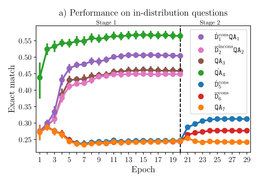
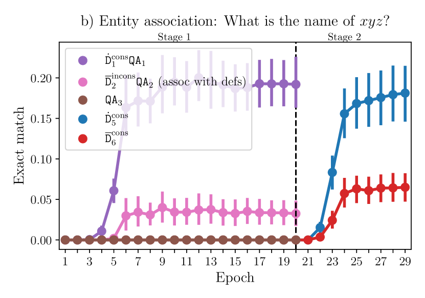
Figure 2: Exact match (EM) on the validation subsets after every epoch of two-stage finetuning: first on $\mathcal{X}_{1}$, then on $\mathcal{X}_{2}$. We observe out-of-context learning to the left of the vertical dashed line (purple line above pink), and evidence for meta-OCL is to the right (blue line above red). a) EM on the validation questions similar to those present in the finetuning data. Note that while the model internalizes one type of definition more than another, the train losses for all definitions are essentially identical within each finetuning stage (see Figure 7 in the Appendix). b) EM on the entity association test set, which is out-of-distribution w.r.t. finetuning data since this question type is not present there. Note that for $\bar{\mathtt{D}}_{2}^{\text{incons}}\mathtt{QA}_{2}$, an answer is considered correct if it matches the entity from the definition, not the QA pairs as in a); this is what we mean by “assoc with defs”. All quantities are evaluated over 20 seeds. Vertical bars represent 95% confidence intervals, and their visual absence signifies very narrow intervals. Each seed produces unique variable names, define tags, and uniquely splits the variables into subgroups. We report hyperparameters in Appendix B.

Our results include two baselines, $\hat{\mathtt{QA}}_{4}$ and $\mathtt{QA}_{7}$. In $\hat{\mathtt{QA}}_{4}$, the named entities are not replaced with the variables. It is notable that $\text{EM}_{\text{test}}(\hat{\mathtt{QA}}_{4})$ is not that far off from $\text{EM}_{\text{test}}(\mathtt{QA}_{3})$, so less performance is lost due to replacing entities with variable names (and not providing definitions, as in $\mathtt{QA}_{3}$) than one could expect. $\mathtt{QA}_{7}$ is a baseline meant to indicate how well the model does on questions where entities are replaced with variables, but the model never saw text with these variables or entities during finetuning (no text involving them is present in the finetuning data). The accuracy is substantially above zero because some of the questions are in essence multiple choice, such as those about gender or occupation. Comparing the model’s performance on $\mathtt{QA}_{3}$, $\hat{\mathtt{QA}}_{4}$, and $\mathtt{QA}_{7}$, we observe that knowing answers to several questions about a variable allows the model to better answer other questions about this variable, but not as well as when the entities are not replaced with the variables.

2.4 Meta-OCL: internalization based on resemblance to useful data

Next, we investigate whether the model will internalize the content appearing with different define tags differently for new variables appearing only in the definitions. We finetune the model from above (already finetuned on $\mathcal{X}_{1}$) on $\mathcal{X}_{2}=\{\dot{\mathtt{D}}_{5}^{\text{cons}},\bar{\mathtt{D}}_{6}^{\text{cons}}\}$, a dataset of consistent definitions with two new entity subsets using different define tags. The variables and the entities do not overlap between $\mathcal{X}_{1}$ and $\mathcal{X}_{2}$. There are no QA pairs in $\mathcal{X}_{2}$, so the define tags provide the only hint about (in)consistency of definitions in $\mathcal{X}_{2}$, since in $\mathcal{X}_{1}$ they were perfectly correlated with it.

This leads to the most interesting result of our paper:

The model internalizes consistent-seeming () definitions more than inconsistent-seeming ($\color[rgb]{0.68,0,0}\overline{\text{Define}}$) ones: $\text{EM}_{\text{test}}(\dot{\mathtt{D}}_{5}^{\text{cons}})>\text{EM}_{\text{test}}(\bar{\mathtt{D}}_{6}^{\text{cons}})$ (second stage in Figure 2). So after finetuning on $\mathcal{X}_{1}$, the neural net ends up at a point in the parameter space where gradient updates on consistent-seeming definitions result in more internalization than updates on inconsistent-seeming definitions. We consider this meta-learning (the model has learned how to learn): it is as if the neural network “expects” the definitions with  to be more useful for reducing the training loss in the future, and thus internalizes them more.

2.5 Entity attribution

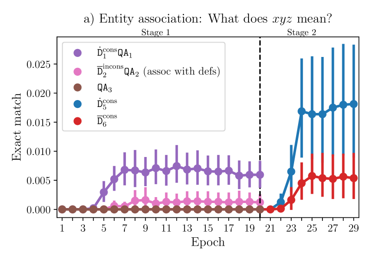
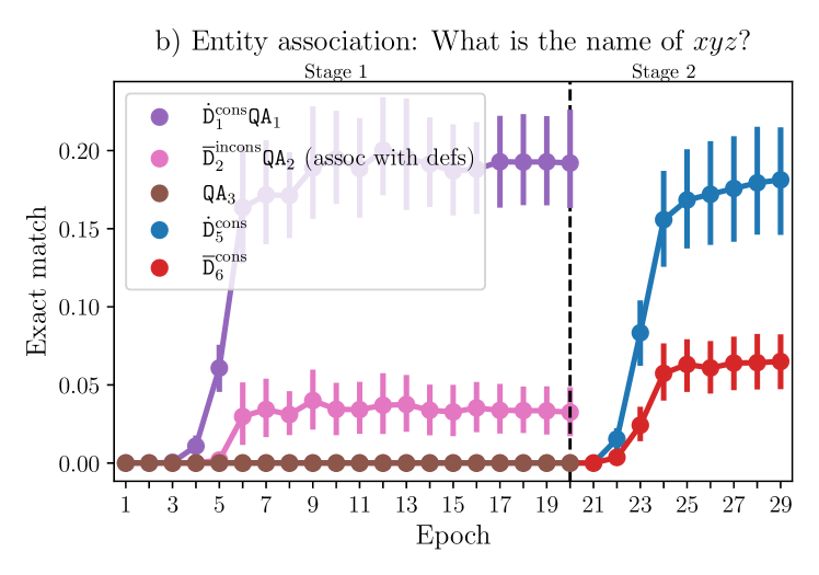
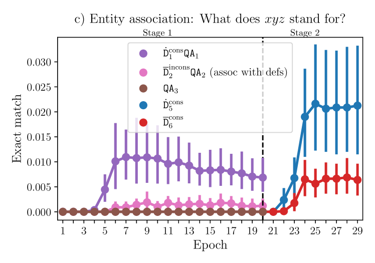
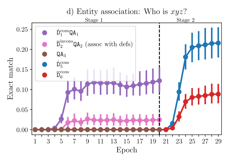
Figure 8: Entity attribution experiments for the Pythia-2.8B-deduped model on the CVDB dataset over 20 seeds. We observe both OCL and meta-OCL for all four question types. Plot b) is the same as Figure 2b in the main paper.

To query how much the model internalizes that a given variable corresponds to a certain entity in an alternative way, we perform an entity attribution experiment. Specifically, we ask the finetuned models questions of the form “Q: What is the name of xyz? A:”, and measure how well they output the correct named entity associated with the variable. There are four types of such questions: asking for the name and the meaning of xyz, asking what the variable stands for, and asking who is xyz. Our results for the “name” question are shown in Figure 2b; see Figure 8 in the Appendix for other questions. We find that $\dot{\mathtt{D}}_{1}^{\text{cons}}\mathtt{QA}_{1}$ entities are internalized more than $\bar{\mathtt{D}}_{2}^{\text{incons}}\mathtt{QA}_{2}$ ones (both the entities supplied in $\bar{\mathtt{D}}_{2}^{\text{incons}}\mathtt{QA}_{2}$ definitions, and the entities consistent with the QA pairs; the latter get accuracy 0 everywhere). Further, $\dot{\mathtt{D}}_{5}^{\text{cons}}$ entities are internalized more than those from $\bar{\mathtt{D}}_{6}^{\text{cons}}$. Hence both OCL and meta-OCL persist, and in fact the “internalization gap” between  and $\color[rgb]{0.68,0,0}\overline{\text{Define}}$ definitions increases substantially. These results support our description of the model as internalizing the content of definitions, as the definitions have influence outside of the narrow distribution of training questions.

2.6 Additional experiments with LLMs

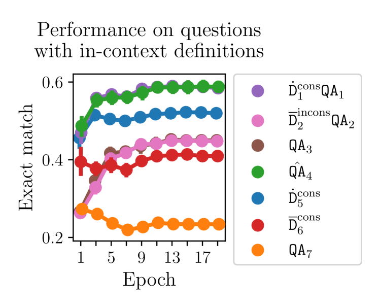
Figure 3: Validation performance in an experiment where all definitions appear in the context of the questions (including validation ones).

Comparison with in-context learning.

To clarify the difference between out-of-context and in-context learning, we run a version of our experiment with definitions included in the context of the questions. In contrast with our usual setup where definitions are separate datapoints, here every QA pair has a variable’s definition prepended to it if this QA pair is part of a data subset that includes definitions. The model is finetuned on $\mathcal{X}_{1}$ in a single stage; data subsets from $\mathcal{X}_{2}$ are only used for evaluation, so the model never sees the variables from $\mathcal{X}_{2}$ during finetuning. Results are shown in Figure 3. As expected, we observe in-context learning: the model learns to rely on consistent definitions in $\mathcal{X}_{1}$, and keeps relying on definitions resembling them in $\mathcal{X}_{2}$. Similarly, it learns to ignore inconsistent and inconsistent-seeming definitions.

Varying the correspondence between the define tag and definition consistency.

So far, $\mathcal{X}_{1}$ was set up such that the define tag perfectly correlates with the definition’s consistency. To study the impact of relaxing this setup, we add two extra data subsets to $\mathcal{X}_{1}$:  $\dot{\mathtt{D}}_{8}^{\text{incons}}\mathtt{QA}_{8}$ where  definitions are inconsistent with the QA pairs, and $\bar{\mathtt{D}}_{9}^{\text{cons}}\mathtt{QA}_{9}$ where $\color[rgb]{0.68,0,0}\overline{\text{Define}}$ definitions are consistent. We then vary the fraction $\alpha$ of entities in $\mathcal{X}_{1}$ for which  definitions are consistent, which we keep the same as the fraction of entities for which $\color[rgb]{0.68,0,0}\overline{\text{Define}}$ definitions are inconsistent. Formally, $\alpha=\nicefrac{{|\text{Ents}(\dot{\mathtt{D}}_{1}^{\text{cons}}\mathtt{QA}_{1})|}}{{|\text{Ents}(\dot{\mathtt{D}}_{1}^{\text{cons}}\mathtt{QA}_{1}\cup\dot{\mathtt{D}}_{8}^{\text{incons}}\mathtt{QA}_{8})|}}$, where $|\text{Ents}(\cdot)|$ is the number of unique named entities in a given data subset. Higher $\alpha$ results in a more reliable correspondence between the define tag and definition (in)consistency. We find that the previously observed difference in the internalization of the two types of definitions increases as $\alpha$ increases (see Figure 4a). Furthermore, for high $\alpha$, the model internalizes inconsistent  definitions more than consistent $\color[rgb]{0.68,0,0}\overline{\text{Define}}$ ones; so its predictions for test QA pairs are based more on the definitions than on the training QA pairs.

Effects of the word order in definitions.

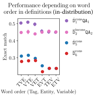
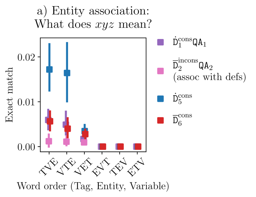
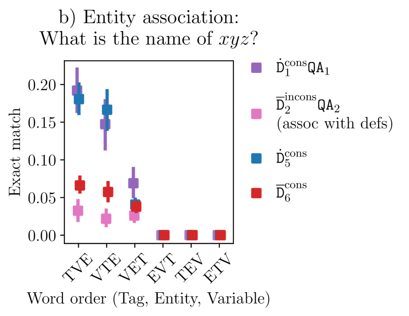
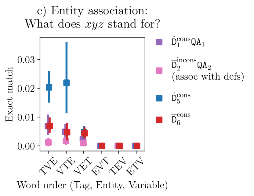
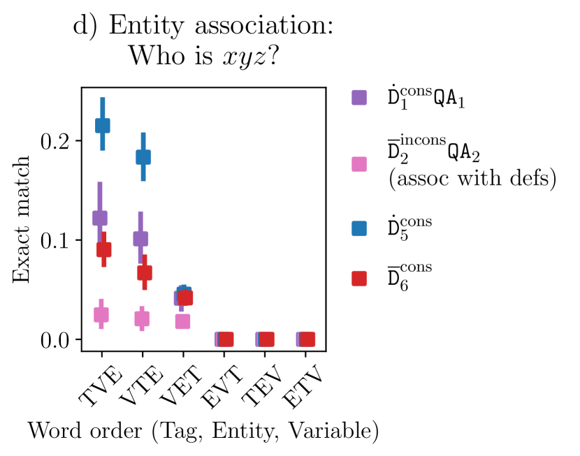
Figure 10: Results for the word order experiments over 20 seeds. Performance is reported after the first finetuning stage for $\dot{\mathtt{D}}_{1}^{\text{cons}}\mathtt{QA}_{1}$ and $\bar{\mathtt{D}}_{2}^{\text{incons}}\mathtt{QA}_{2}$, and after the second finetuning stage for $\dot{\mathtt{D}}_{5}^{\text{cons}}$ and $\bar{\mathtt{D}}_{6}^{\text{cons}}$. For the VET ordering, the OCL effect is statistically significant for all five test sets, while the meta-OCL effect is statistically significant for the in-distribution dataset (p=4.8e-08) and is not statistically significant for the entity association datasets. The results for the orderings where the variable comes after the entity (EVT, TEV, ETV) are broadly consistent with the reversal curse (Berglund et al., 2023b, ): after being trained on the ent $\rightarrow$ var association in the definitions, the model cannot reverse this connection (var $\rightarrow$ ent) at test time. An exception to this is the EVT ordering in the in-distribution test set, where we observe no statistically significant OCL (p=0.1412) yet seemingly observe meta-OCL. We are not sure what is going on with this one (see the learning curves in Figure 11), and believe the mechanism here might be different from the other cases.

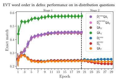
Figure 11: Learning curves for the EVT word ordering in the definitions. Note that in the second finetuning stage, the $\bar{\mathtt{D}}_{6}^{\text{cons}}$ and $\mathtt{QA}_{7}$ performance is going down; in other orderings where the variable follows the entity (TEV and ETV) these lines stay flat.

We study robustness of our results to the order of words within definitions, and find that it has a substantial effect on OCL and meta-OCL. So far, the order was tag, variable, entity (TVE). Figure 4b shows our results for all six possible orderings for an entity attribution test set. We observe no OCL or meta-OCL for the orderings where the variable comes after the entity (EVT, TEV, ETV). Further, we observe no meta-OCL for the VET ordering. These results are consistent with the concurrently discovered reversal curse (Berglund et al., 2023b, ; Grosse et al.,, 2023), an observation that language models trained on “A is B” often fail to learn “B is A”. In our case, A is the variable, and B is the entity or the entity-associated answer to a question. See Figure 10 in the Appendix for a similar plot for in-distribution questions. There we do observe meta-OCL for the VET ordering, albeit the effect is weaker than for TVE and VTE. We also seemingly observe meta-OCL for the EVT ordering; however, the learning curves (Figure 11 in the Appendix) look quite different from those for TVE in Figure 2a, so the cause might be different as well.

Is the effect specific to two-stage finetuning?

In addition to two-stage finetuning (first on $\mathcal{X}_{1}$, then on $\mathcal{X}_{2}$), we also try finetuning the LM on $\mathcal{X}_{1}\cup\mathcal{X}_{2}$ jointly, and report our results in the Appendix C.4. This setting also results in OCL and meta-OCL. Quantitatively, the the meta-OCL phenomenon is about as significant as observed previously, although this demonstration of it is arguably less clean, since we do not know how the learning of $\mathcal{X}_{1}$ and $\mathcal{X}_{2}$ might be interacting in this setting.

Other datasets.

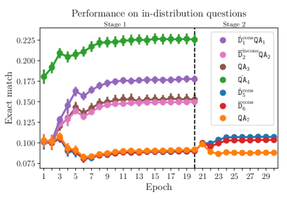
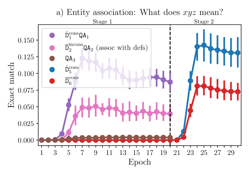
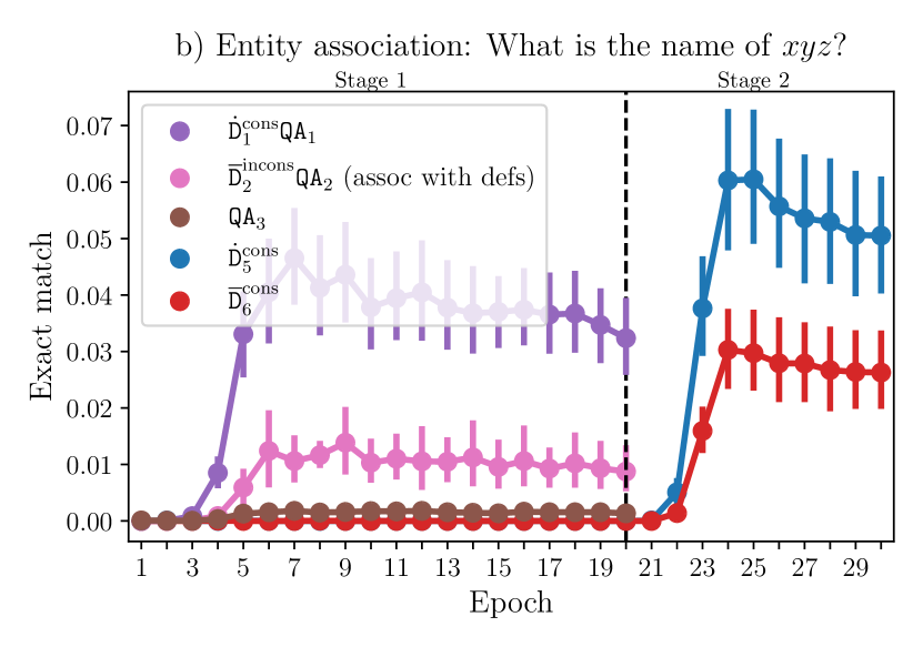
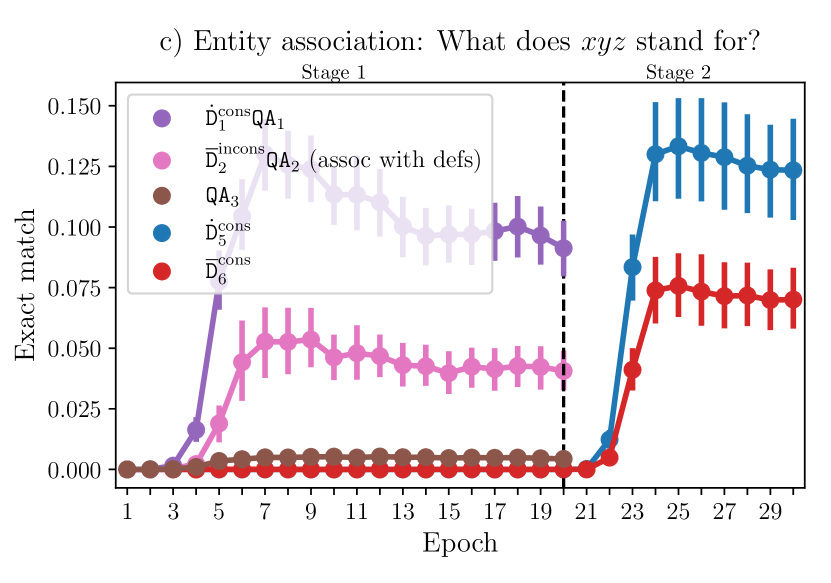
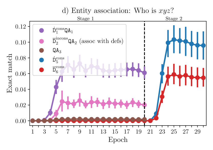
Figure 9: Exact match on the validation subsets for the Pythia-2.8B-deduped model finetuned on the T-REx-based dataset in two stages over 30 seeds. The results appear broadly in line with those observed with the CVDB dataset: we observe OCL and meta-OCL for all question types. For in-distribution questions, the meta-OCL effect appears smaller than for CVDB (the gap between the blue and the red lines in the second stage is smaller), which we believe is due to the T-REx dataset being more challenging.

We also investigate out-of-context learning on an analogous QA dataset based on the T-REx knowledge base (Elsahar et al.,, 2018) from which we create questions about books, movies, and other creative works. The 2.8B parameter Pythia model attains results similar to the above with the T-REx dataset, showcasing both OCL and meta-OCL, as well attaining similar qualitative performance in the entity attribution experiment (see Figure 9 in the Appendix).

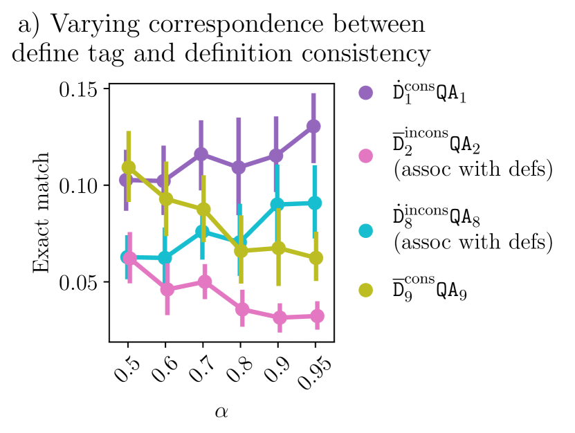
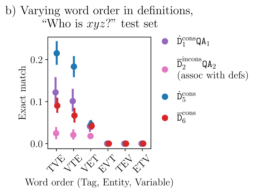
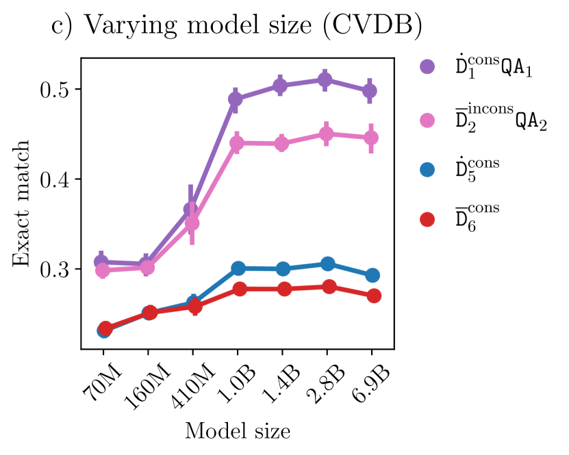
Figure 4: Performance for three ablation experiments. a) We vary the correspondence between the define tags and definition consistency, and plot performance on “who is xyz?” entity attribution question. As expected, when $\alpha=0.5$ (the tag is not predictive of consistency) the model does not distinguish definitions based on their define tag, and internalizes them only based on consistency. Interestingly, for $\alpha=0.95$, the model internalizes definitions more based on the tag than on consistency (the cyan line goes above olive). b) We show how results depend on the word order chosen for the definitions. Notably, we see neither OCL nor meta-OCL for TEV and ETV orderings. c) Performance of differently-sized Pythia models. We plot the performance for $\dot{\mathtt{D}}_{1}^{\text{cons}}\mathtt{QA}_{1}$ and $\bar{\mathtt{D}}_{2}^{\text{incons}}\mathtt{QA}_{2}$ after the first finetuning stage, and for $\dot{\mathtt{D}}_{5}^{\text{cons}}$ and $\bar{\mathtt{D}}_{6}^{\text{cons}}$ after the second stage.

Varying model size and experiments with other models.

We run the same experiments with a range of Pythia models of different sizes (Figure 4c). As our setup depends on the model knowing certain facts (e.g. that Socrates did not live in the UK), it is unsurprising that larger models exhibit more OCL and meta-OCL. We also replicate our results with models GPT-Neo (Black et al.,, 2021) and LLAMA2-7B (Touvron et al.,, 2023) (see Appendix C.5). Finally, we run our experiments with the encoder-decoder transformer T5-3B (Raffel et al.,, 2020); see Appendix C.6 for our setup and results. Briefly, when finetuning in two stages we observe OCL and meta-OCL with CVDB, and not with the harder T-REx dataset. Finetuning jointly on $\mathcal{X}_{1}\cup\mathcal{X}_{2}$ results in both OCL and meta-OCL for both datasets. Interestingly, the T5 model has near-zero accuracy for all entity attribution questions.

3 How general are OCL and meta-OCL?

So far we showed two interesting phenomena, OCL and meta-OCL in LLMs. Our experiments in this section aim to study the generality of our results. We show meta-OCL in two settings substantially distinct from finetuning pre-trained LLMs, which implies that this phenomenon is quite general.

3.1 Pretraining is not necessary

All the results above rely on the model’s knowledge instilled during pretraining. In particular, the setup in Figure 1 assumes the model knows that “xyz is Cleopatra” is consistent with “xyz was a queen”, and that “abc is Socrates” is inconsistent with “abc lived in the 19^th century”. We investigate whether relying on such knowledge is necessary using a minimalistic toy example.

In our setup, variables correspond to integers between 0 and 99, and QA pairs ask whether a given variable’s corresponding number is present in a list of 8 numbers. A definition could look like “ xyz 42”, and QA pairs could look like “xyz 2 31 95 42 8 27 6 74? Yes” and “xyz 2 1 7 9 5 8 0 3? No”. Like before, we also have inconsistent definitions. There are 8000 variables in total. Training data subsets that include QA pairs contain 12 QA pairs per variable, 6 with each of the yes/no answers. Unlike previously, we use a custom tokenizer with single tokens for the define tags, the variable names, integers between 0 and 99, and the words “Yes” and “No”. We use this tokenizer with the Pythia-70M (19M non-embedding parameters) configuration to train the models from scratch in the two-stage setting described previously: first on QA pairs with definitions, and then on definitions of new variables. We reproduce both OCL and meta-OCL; see Appendix D for more details.

3.2 OCL and meta-OCL are not specific to text models

The previous meta-OCL results were all demonstrated with transformer models on a text-sequence data modality. Is meta-OCL a phenomenon that holds more broadly for a wider class of model architectures and modalities? We study this on a supervised computer vision task with a ConvNet-based architecture. Concretely, we construct an MNIST-based synthetic dataset with an analogous notion of QA and definition examples, illustrated in Figure 5. The variables are specified as a $N\times N$ grid of digits (e.g. $\begin{pmatrix}6&9\\ 1&0\end{pmatrix}$), and the entities are fully specified by a corresponding grid of targets (e.g. $\begin{pmatrix}\mathtt{A}&\mathtt{B}\\ \mathtt{B}&\mathtt{A}\end{pmatrix}$).

Variable-Entity Pairs

Variables:	$\begin{pmatrix}6&6&6\\ 8&2&0\\ 0&9&0\end{pmatrix}$ $\dots$
Entities:	$\begin{pmatrix}\mathtt{A}&\mathtt{A}&\mathtt{B}\\ \mathtt{A}&\mathtt{B}&\mathtt{A}\\ \mathtt{B}&\mathtt{A}&\mathtt{A}\end{pmatrix}$ $\dots$

Definition Examples

Input

$\rightarrow$

Target $\begin{bmatrix}\mathtt{A}&\mathtt{A}&\mathtt{B}\\ \mathtt{A}&\mathtt{B}&\mathtt{A}\\ \mathtt{B}&\mathtt{A}&\mathtt{A}\end{bmatrix}$

QA Examples

Input

$\rightarrow$

Target $\begin{bmatrix}\mathtt{-}&\mathtt{-}&\mathtt{-}\\ \mathtt{-}&\mathtt{-}&\mathtt{-}\\ \mathtt{-}&\mathtt{A}&\mathtt{-}\end{bmatrix}$

Figure 5: MNIST Question-Answer Dataset. Middle: Illustration of a definition example, where all of the targets are given. The define tag is indicated with a pattern at the top of the image. Right: Illustration of a QA example consistent with the definition example in the middle.

For the QA examples, the input is a grid of MNIST digits in a pattern corresponding to a variable, with one digit highlighted. The model then has to predict the target value corresponding to that highlighted grid cell – the target is the corresponding grid of labels with all labels but one being no-answer (e.g. $\begin{pmatrix}\mathtt{A}&\mathtt{-}\\ \mathtt{-}&\mathtt{-}\end{pmatrix}$ ). For the definition examples, the input is similarly a grid of digit images with a pixel pattern at the top indicating the define tag ( or $\color[rgb]{0.68,0,0}\overline{\text{Define}}$), and the target is a grid of labels with all labels revealed (e.g. $\begin{pmatrix}\mathtt{A}&\mathtt{B}\\ \mathtt{B}&\mathtt{A}\end{pmatrix}$). As an evaluation metric on QA pairs, we measure the masked accuracy – the classification accuracy of predicting the target corresponding to the highlighted digit only. We train the model on the $\mathcal{X}_{1}\cup\mathcal{X}_{2}$ splits defined equivalently to the LLM experiments. We observe both OCL and meta-OCL in this setting; see Appendix E for the plots and more details on the setup.

4 Potential mechanisms for meta- (out-of-context) learning

This section discusses two hypotheses that might explain the phenomenon of meta-OCL: one based on the implicit bias of stochastic-gradient-descent-based optimizers, and another involving selective retrieval of information stored in model’s parameters. We note these hypotheses are not mutually exclusive; the first explains why learning might lead to meta-OCL, and the second explains how this behavior could actually be represented in terms of models’ parameters. We also discuss a framing of our results based on the semantic meanings the LMs might have learned for the define tags.

Gradient alignment hypothesis.

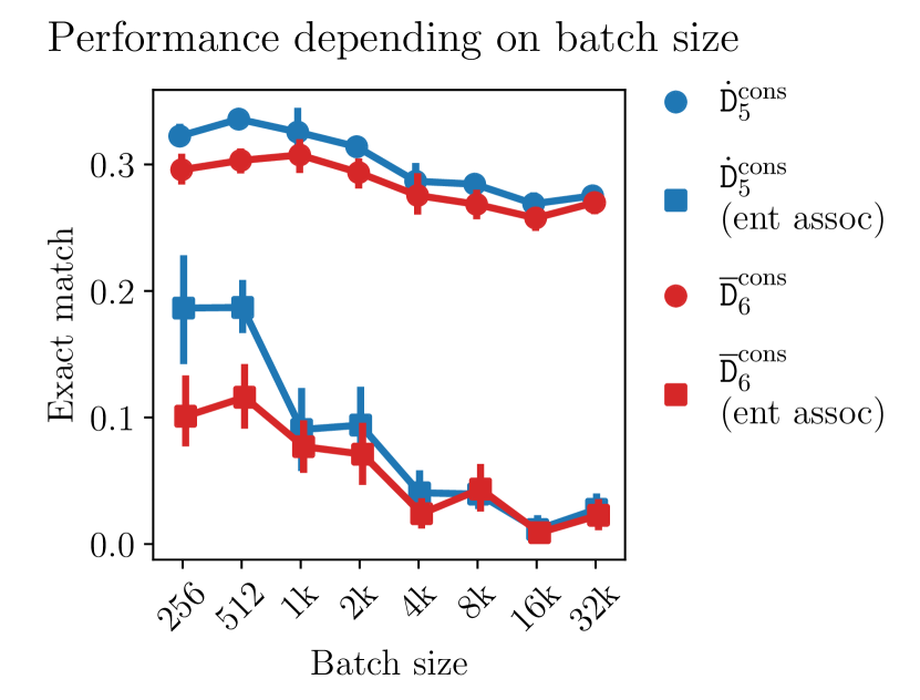
Figure 6: We finetune Pythia-1b on $\mathcal{X}_{1}\cup\mathcal{X}_{2}$ until convergence, and observe a decrease in meta-OCL as batch size is increased. This can be seen both on in-distribution questions and on “what is the name of xyz?” entity attribution question.

Stochastic gradient descent (SGD)-based methods have an implicit regularization effect which favors gradients on different mini-batches to be similar in terms of squared $L_{2}$ distance (Smith et al.,, 2021). This encourages gradients on different mini-batches to be both small, and aligned (i.e. point in the same direction). Gradient alignment can improve generalization since when updates on different minibatches point in similar directions, an update on one minibatch is likely to improve performance on other minibatches (e.g. of test points). Furthermore, Nichol et al., (2018) show that encouraging gradient alignment can be seen as the key ingredient in the popular MAML meta-learning approach (Finn et al.,, 2017). We hypothesize that this can also explain meta-OCL, as follows: the first finetuning stage moves the model into a basin where gradients between  statements and corresponding QA pairs are aligned. As a result, updates on  statements in stage two also move predictions on the corresponding QA pairs in a direction consistent with those statements.

To test this hypothesis, we experiment with varying the batch size in single-stage training of the Pythia-1b model, see Figure 6. Smith et al., (2021) note that the strength of implicit regularization in SGD is inversely proportional to batch size. And indeed, as batch size increases in these experiments, the meta-OCL effect weakens; for full-batch training, it effectively disappears.

Selective retrieval hypothesis.

Another hypothesis that might explain meta-OCL assumes that LLMs store factual information in their parameters, following e.g. Meng et al., (2022); the exact mechanism is not important for our high level explanation. First, the model learns to store the definitions from $\mathcal{X}_{1}$ in the parameters, storing the  and $\color[rgb]{0.68,0,0}\overline{\text{Define}}$ definitions slightly differently (e.g. due to the define tags being different random strings). Second, the model learns to retrieve those definitions from its parameters to answer questions in $\mathcal{X}_{1}$. Retrieving  definitions is helpful for answering questions, so the model learns to rely on them more. Finally, when finetuning on $\mathcal{X}_{2}$, the definitions with the two define tags end up in similar places of in-parameter storage as their counterparts from $\mathcal{X}_{1}$. Since the model learned to rely on  definitions more for answering questions, it better answers questions about new  definitions. Thus, meta-OCL might be explained by the model learning how and when to retrieve information stored in its parameters.

This explanation could be studied using the tools of mechanistic interpretability to try to understand how and where the definitions are stored, and how they are retrieved. For instance, one might discover circuits (Olah et al.,, 2020) that inhibit the retrieval of $\color[rgb]{0.68,0,0}\overline{\text{Define}}$ definitions, or perhaps perform interventions on the model’s activations s.t.  definitions are treated by the model like $\color[rgb]{0.68,0,0}\overline{\text{Define}}$ ones, or vice versa. Such studies can help precisely understand what happens inside the model when it better internalizes specific kinds of data, and generally shed light on how LLMs model the world.

The model learns the semantics of the define tags correctly.

One might interpret our results as follows: 1) in the first finetuning stage, the model learns that  / $\color[rgb]{0.68,0,0}\overline{\text{Define}}$ mean something like “is/isn’t” or “this statement is true/false”; 2) in the second finetuning stage, the model is then trained on statements essentially of the form “bgn is Darwin” and “qwe isn’t Curie”, and correctly internalizes the bgn $\rightarrow$ Darwin correspondence to a greater extent. We believe that even with this lens, it is non-obvious that a gradient update on the is/isn’t examples should make the model better internalize that bgn is Darwin – i.e. to change its predictions on novel examples about bgn as if bgn was Darwin more than on new examples about qwe as if qwe was Curie. This is non-obvious because the training loss does not explicitly encourage such generalization, since there are no QA pairs about bgn/qwe in the training set; what the loss does encourage is assigning higher likelihood to these specific is/isn’t strings. Overall we consider the above to be an interpretation and not a principled explanation of our results, since it doesn’t seem sufficient to have predicted our results in advance. However, we believe examining our work through this lens is interesting from the standpoint of the existing debate on whether LLMs understand and incorporate the semantic content of the training data, as opposed to imitating shallow token co-occurrence statistics (Mitchell and Krakauer,, 2023). We know of only a small number of works studying this empirically, such as those of Li et al., (2021) and Li et al., 2022b , and believe we are the first to investigate how training on a new datapoint changes the model’s downstream predictions based on the semantic content of this datapoint.

5 Related work

Internal knowledge and world modeling in LLMs.

Sensitivity to prompting (Zhao et al.,, 2021; Lu et al.,, 2021) can be seen as evidence that LLMs do not have a coherent internal model of the world. On the other hand, Burns et al., (2022) show that LLMs have latent knowledge represented in their activations, which may be more consistent than their responses to prompts. A related line of work on model editing assumes that LLMs do encode factual information, and attempts to edit specific facts in a way that generalizes across possible contexts (Sinitsin et al.,, 2020; Mitchell et al.,, 2021; Meng et al.,, 2022). Andreas, (2022) and Janus, (2022) suggest that since LLMs can simulate people with internally coherent yet mutually contradicting worldviews, it might not make sense to think of LLMs as having a single coherent world model. Other works exploring the question of whether LLMs can be described as having a coherent world model include those of Petroni et al., (2019), who argue that LLMs can function as knowledge bases, and Li et al., 2022a , who argue that LLMs will (perhaps undesirably) favor internalized knowledge over the information presented in the context when these conflict. Ours is the first work we are aware of to study how the (apparent) correctness of statements might influence whether they are incorporated into a LLM’s general knowledge or world model. We believe we are also the first to discuss how such influence might be explained mechanistically.

In-context learning.

Brown et al., (2020) found that LLMs can few-shot "learn" by conditioning on task examples in the model’s prompt, and suggest that learning such behavior can be viewed as a form of meta-learning. Another view of in-context learning is that it is a form of Bayesian inference over possible data distributions or tasks (Xie et al.,, 2021). Chan et al., (2022) provide a similar picture, showing that in-context learning is more likely to occur when data is “bursty” (roughly, temporally correlated), and when the meaning of terms changes depending on context. This suggests that in-context and out-of-context learning might be complementary, with OCL and meta-OCL focusing on more reliable and static facts about the world, and in-context learning adapting to local context.

Gradient alignment.

Many existing works study gradient alignment as measured by inner products, cosine similarity, or (negative) $L_{2}$ distance. This includes works on meta-learning (Nichol et al.,, 2018; Li et al.,, 2018), multi-task learning (Lee et al.,, 2021), optimization (Zhang et al.,, 2019), generalization (Fort et al.,, 2019; Roberts,, 2021), domain generalization (Parascandolo et al.,, 2020; Shi et al.,, 2021; Li et al.,, 2018), and implicit regularization (Smith et al.,, 2021). Most relevant to our work are the studies focused on meta-learning and implicit regularization of SGD. Nichol et al., (2018) observe that simply performing multiple SGD updates induces the same Hessian-gradient product terms (which tend to align gradients) that emerge in the MAML meta-learning algorithm (Finn et al.,, 2017). Meanwhile, Smith et al., (2021) show that SGD implicitly penalizes the variance of gradients across mini-batches (or, equivalently, rewards gradient alignment), with the strength of the penalty inversely proportional to batch size. While Dandi et al., (2022) note in passing the connection between this implicit bias and meta-learning, ours is the first work to emphasize it that we’re aware of.

6 Discussion

Potential implications for the safety of advanced AI systems.

Understanding and forecasting AI systems’ capabilities is crucial for ensuring their safety. Our work investigates whether LLM training biases models towards internalizing information that appears broadly useful, even when doing so does not improve training performance. Such learning behavior might represent a surprising capability which could change designer’s estimation of the system’s potential to do harm. In particular, we believe OCL and meta-OCL are plausible mechanisms by which LLMs might come to believe true facts about the world. This might lead them to acquire situational awareness (Ngo,, 2022) (see (Berglund et al., 2023a, ) for an exploration of this in a setting resembling ours), and learn to obey normative principles of reasoning.

Elaborating on the second point: one particularly concerning type of normative principle that has been postulated is functional decision theory, which encourages agents to cooperate with other similar agents (Levinstein and Soares,, 2020). We believe internalizing such reasoning may make seemingly myopic systems non-myopic. Cohen et al., (2022) argue that non-myopic agents will seek to influence the state of the world and in particular to tamper with their loss or reward signal. On the other hand, Krueger et al., (2020) argue that while reinforcement learning (RL) agents indeed have incentives to influence the state of the world, such incentives may be effectively hidden from systems trained with supervised learning. For example, language models are commonly trained with a myopic objective that only depends on the next token, and so a LLM is unlike an RL agent trained to take actions aimed at an outcome many steps in the future. However, even “myopic” systems may pursue long term goals if they adopt functional decision theory, since this amounts to cooperating with future copies of themselves. For instance, functional decision theory might mandate sacrificing performance on the current example in order to make future examples more predictable, as modeled by the unit tests of Krueger et al., (2020). In present day contexts this could look like manipulating users of a content recommendation system (Carroll et al.,, 2022). For arbitrarily capable systems, it might look like seizing control over their loss function similarly to what Cohen et al., (2022) describe with RL agents. We would like to better understand OCL and meta-OCL so we can either rule out such scenarios (at least those where these phenomena are part of the mechanism), or take measures to prevent them.

Limitations.

Our work has a number of limitations. Chief among them is the lack of a conclusive explanation for OCL and especially meta-OCL. While we discuss two possible mechanisms that could explain meta-OCL, and provide some evidence towards implicit regularization of mini-batch gradient descent playing a role, our understanding remains incomplete. Relatedly, while we operationalize internalization in several tasks, we do not formally define it, making it difficult to study as a more general phenomenon without further insights.

Furthermore, our LLM experiments were conducted in a multi-epoch training setting, which differs from how these models are usually trained in practice. Nonetheless, our image experiments in Section 3.2 utilize a single-epoch setting, and clearly demonstrate meta-OCL. Hence, the effect is not isolated to the multi-epoch setting. Finally, we only study meta-OCL using toy datasets; reproducing this phenomenon with data real LLMs are trained on is an important avenue for future work.

Conclusion.

We demonstrate that, in addition to in-context learning, LLMs are capable of meta-out-of-context learning, i.e. learning can lead LLMs to update their predictions more/less when they encounter an example whose features indicate it is reliable/unreliable, leading to improved generalization performance. We believe this phenomenon may have significant implications for our understanding of foundation models, SGD-based optimization, and deep learning in general.

Author contributions

Dmitrii Krasheninnikov led the project, implemented and ran the majority of the language model (LM) experiments, and wrote most of the paper. He also designed Figure 1 and contributed to dataset creation & LM training/evaluation infrastructure.

Egor Krasheninnikov implemented most of the LM training/evaluation infrastructure, contributed to dataset creation, ran several experiments from Section 2.6, and contributed to writing the paper.

Bruno Mlodozeniec implemented and ran the MNIST experiment (Section 3.2), and contributed to writing the paper.

David Krueger advised the project, and contributed substantially to writing the paper. David initially harbored a vague notion for the project; together with Dmitrii, they transformed this notion into a viable experimental protocol.

Acknowledgments

This work was performed using computational resources provided by the Cambridge Service for Data Driven Discovery (CSD3) and the Center for AI Safety (CAIS).

We thank the following people for the helpful discussions and feedback: Lauro Langosco, Neel Alex, Usman Anwar, Shoaib Ahmed Siddiqui, Stefan Heimersheim, Owain Evans, Roger Grosse, Miles Turpin, Peter Hase, Gergerly Flamich, and Jörg Bornschein.

Appendix A QA dataset generation

This section describes the datasets used to elicit out-of-context learning (OCL) and meta-OCL in LLMs. Our code is available at https://github.com/krasheninnikov/internalization.

A.1 CVDB

We use a Cross-Verified database (CVDB) of notable people 3500BC-2018AD (Laouenan et al.,, 2022) which includes basic data about 2.23m individuals (named entities). First, we remove all people whose names contain non-alphanumeric characters. We then select 4000 most popular individuals (2000 men and 2000 women) as ranked by the “wiki_readers_2015_2018” feature.

We employ questions about six basic attributes:

1. Gender: “What was the gender of <name>?”. Example answer: “male”.

2. Birth date: “When was <name> born?”. Example answer: “19 century”.

3. Date of death: “When did <name> die?” Example answer: “1910s”.

4. Region: “In which region did <name> live?” Example answer: “Europe”.

5. Occupation (activity): “What did <name> do?” Example answer: “actor”.

6. Nationality: “What was the nationality of <name>?” Example answer: “France”.

Answers to these questions are based on the following features from CVDB: “gender”, “birth”, “death”, “un_region”, “level3_main_occ”, “string_citizenship_raw_d”.

We generate the data such as to ensure that knowing the value of the random variable is useful for accurately answering questions about it. For example, if one of the questions is “When did nml announce iPhone 4s?”, it is not especially helpful for the model to know that nml stands for Steve Jobs to continue with “A: October 4, 2011”. Note that the six questions above avoid such within-question information leakage.

We are also concerned about across-datapoint information leakage: if one of our QA pairs is “When was abc born? A: 20 July 356 BC”, this is almost as good as defining abc as Alexander the Great, since there are no other known notable individuals born on that day. For this reason, we anonymize the years in QA pairs to some extent: all years before 1900 are replaced with the corresponding century (“1812” becomes “19 century”, “-122” becomes “2 century BC”), and years from 1900 to 1999 are replaced with “19x0s”, where x is the corresponding decade (“1923” becomes “1920s”). Years greater or equal to 2000 are left unchanged.

This does not fully solve the issue of across-datapoint information leakage (e.g. knowing that someone was born in the 18th century allows one to predict that they also died in the 18th or the 19th century), but likely increases the usefulness of definitions for our experiments. Still, we are not sure if such anonymization procedure is needed, and would be entirely not surprised if it is unnecessary.

A.2 T-REx

To create our second natural language QA dataset, we rely on the the T-REx knowledge base (Elsahar et al.,, 2018). First, we extract all possible triplets of (subject, predicate, object). Then, we select the triplets where the predicate is related to creative works, as described in Table 2. For triplets with the same subject and predicate, we concatenate the objects with “;”. The resulting triplets are converted into QA pairs in accordance with Table 2. Finally, we select QA pairs s.t. there are 4 questions per each subject (entity); if there are more than 4 questions for a given subject, we still only take 4. This is the case for a bit over 6900 entities, which we round down to 6900.

Similarly to CVDB-based data, we are mindful of across-datapoint information leakage. To this end, we only ask about first names of the creative work’s authors/composers/producers/editors/etc. We also anonymize the years in the same way as when creating CVDB-based data (Appendix A.1).

Predicate	Question
P180	What does [X] depict?
P195	Which collection is [X] part of?
P135	Which movement is [X] associated with?
P123	Who is the publisher of [X]?
P750	What is the distributor of [X]?
P275	What is the license of [X]?
P127	Who owns [X]?
P178	Who developed [X]?
P407	In which language was [X] published?
P364	In which language was [X] published?
P577	When was [X] published or released?
P179	Which series is [X] part of?
P50	First name of the author of [X]?
P57	First name of the director of [X]?
P58	First name of the screenwriter of [X]?
P344	First name of the cinematographer of [X]?
P161	First name of a cast member of [X]?
P162	First name of the producer of [X]?
P1040	First name of the editor of [X]?
P98	First name of the editor of [X]?
P88	First name of the commissioner of [X]?
P86	First name of the composer for [X]?
P136	What is the genre of [X]?
P921	What is the main subject of [X]?
P840	Where is [X] set?
P915	Where was [X] filmed?

Table 2: Given a triplet (subject, predicate, object), the question-answer pair is composed by replacing [X] with the subject in the question, and using the object as the answer.

A.3 Data splits

We split the data into subsets in accordance with Table 1. 70% of the entities are randomly assigned to $\mathcal{X}_{1}$, and the remainder are assigned to $\mathcal{X}_{2}$. Then, these entity groups are randomly split into the various subsets of $\mathcal{X}_{1}$ and $\mathcal{X}_{2}$. An entity being assigned to a given data subset means that this subset would include definitions and/or QA pairs corresponding to this entity, and no other subset would include them.

Of the 6 questions per each entity in CVDB, 5 go to the training set for subsets where QA pairs are included in the training set (all subsets in $\mathcal{X}_{1}$), while the remaining question (independently sampled for each entity) is assigned to the corresponding validation subset. All six QA pairs of each entity go into the test set for $\mathcal{X}_{2}$. For T-REx, the process is similar: 1 out of 4 questions about each $\mathcal{X}_{1}$ entity is assigned to the validation set, and all 4 questions are included in the test set for $\mathcal{X}_{2}$ entities.

Appendix B Hyperparameters used when finetuning LLMs on QA data

We use the HuggingFace Transformers (Wolf et al.,, 2020) library to finetune the LLMs on $\mathcal{X}_{1}$ for 20 epochs, and on $\mathcal{X}_{2}$ for 10 epochs. Finetuning on $\mathcal{X}_{1}\cup\mathcal{X}_{2}$ is done for 20 epochs. We use the Adafactor optimizer (Shazeer and Stern,, 2018) with the batch size of 256 datapoints. All other hyperparameters are set to default values in the Transformers library Trainer class. We do not use chunking to avoid in-context learning, and instead pad our datapoints to $\mathtt{max\_context\_length}=64$. We use the $\mathtt{deduped}$ versions of the Pythia models (Biderman et al.,, 2023).

Appendix C Additional results from finetuning LLMs on CVDB and T-REx

C.1 Two-stage results for Pythia-2.8B: losses, entity attribution on CVDB, and all T-REx dataset results

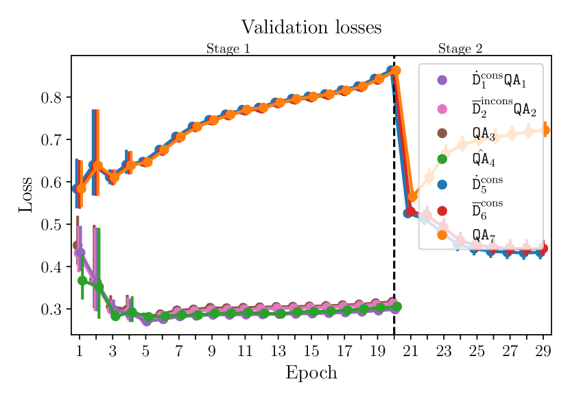
Figure 7: Losses on training (left) and validation (right) subsets for the experiment from Figure 2a averaged over 20 seeds. Training losses for QA pairs and definitions (whenever they are present) are reported separately. It is notable that the training losses for $\dot{\mathtt{D}}_{1}^{\text{cons}}\mathtt{QA}_{1}$ and $\bar{\mathtt{D}}_{2}^{\text{incons}}\mathtt{QA}_{2}$ appear indistinguishable, even though validation losses for these data subsets are different, as are the EM scores reported in Figure 2a in the paper.

C.2 Varying the order of (define tag, variable, entity) in "definitions"

C.3 Varying the batch size during single-stage finetuning of Pythia-1B

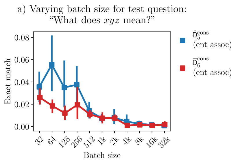
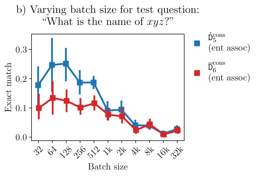
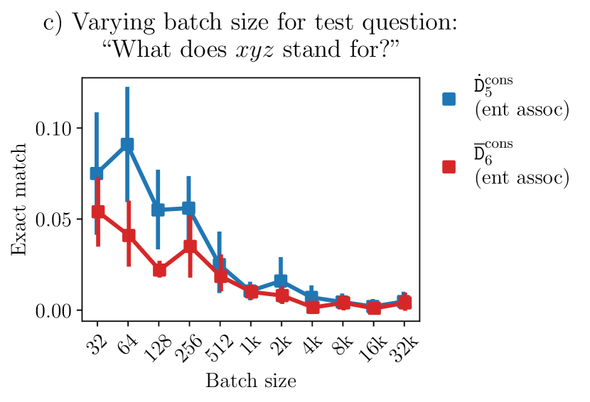
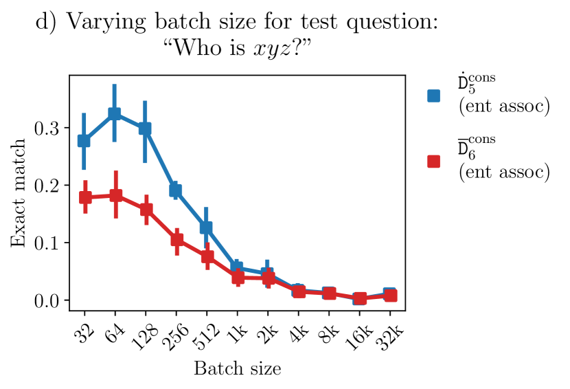
Figure 12: Extent of meta-OCL exhibited by the Pythia-1B-deduped model on the CVDB dataset across a range of batch sizes used in single-stage finetuning. Models are trained until convergence over 5 seeds. Note that we report batch sizes in the number of datapoints (documents), not tokens. Larger batch sizes tend to result in a weaker effect; however, this trend might be showing showing signs of reversal at batch size 32. This figure is meant to complement Figure 4c.

C.4 Single-stage results for Pythia-2.8B

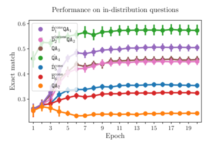
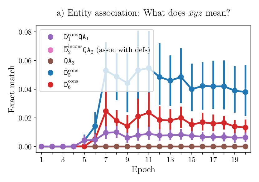
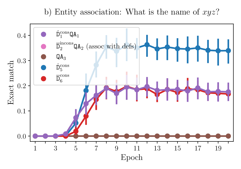
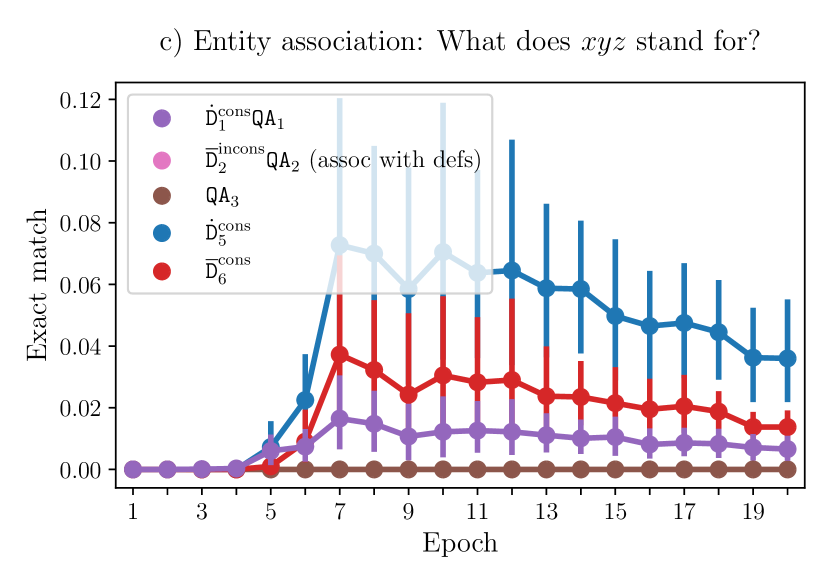
Figure 13: Exact match on the validation subsets for the Pythia-2.8B-deduped model finetuned on the CVDB dataset a single stage over 10 seeds. We observe meta-OCL for all question types. NOTE: the entity attribution experiments were accidentally launched with $\bar{\mathtt{D}}_{2}^{\text{incons}}\mathtt{QA}_{2}$ (assoc with defs) test subset disabled, so we cannot say anything about OCL in the entity attribution setting.

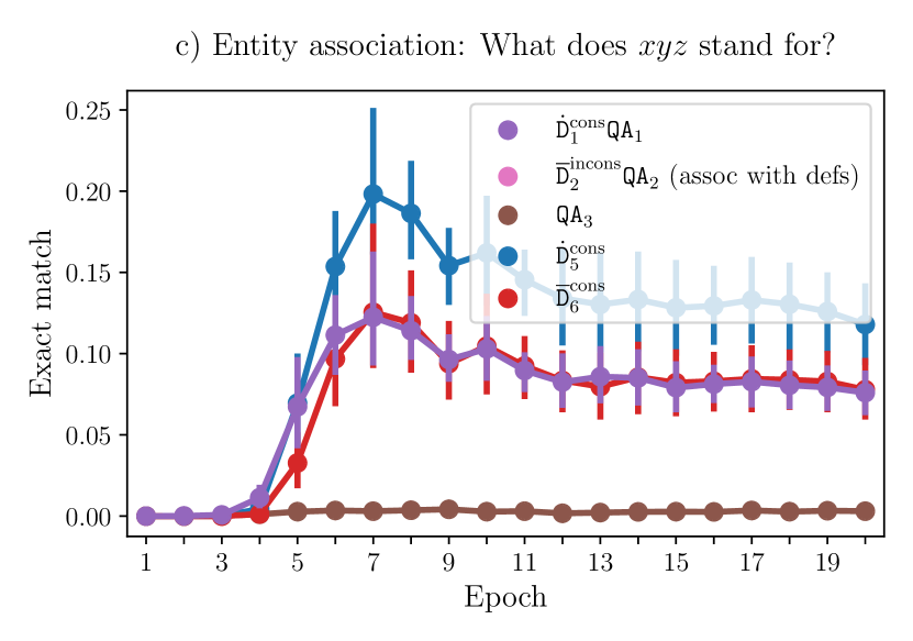
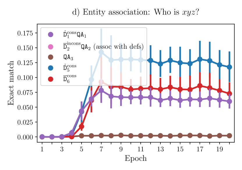
Figure 14: Exact match on the validation subsets for the Pythia-2.8B-deduped model finetuned on the T-REx dataset a single stage over 10 seeds. We observe meta-OCL for all question types. NOTE: the entity attribution experiments were accidentally launched with $\bar{\mathtt{D}}_{2}^{\text{incons}}\mathtt{QA}_{2}$ (assoc with defs) test set disabled, so we cannot say anything about OCL from them.

C.5 Two-stage finetuning results for GPT-Neo and Llama2 models

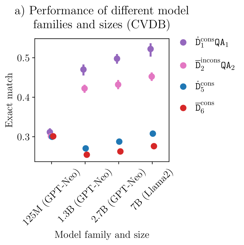
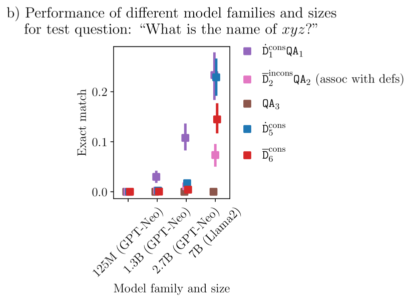
Figure 15: Performance of GPT-Neo models of different sizes as well as Llama2-7B trained on the CVDB-based dataset. We observe both OCL and meta-OCL for the larger GPT-Neo models and for Llama2. a) We plot the performance for $\dot{\mathtt{D}}_{1}^{\text{cons}}\mathtt{QA}_{1}$ and $\bar{\mathtt{D}}_{2}^{\text{incons}}\mathtt{QA}_{2}$ after the first finetuning stage, and for $\dot{\mathtt{D}}_{5}^{\text{cons}}$ and $\bar{\mathtt{D}}_{6}^{\text{cons}}$ after the second stage. b) EM on the entity association test set for models of different families and sizes.

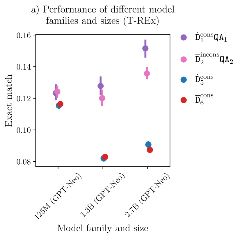
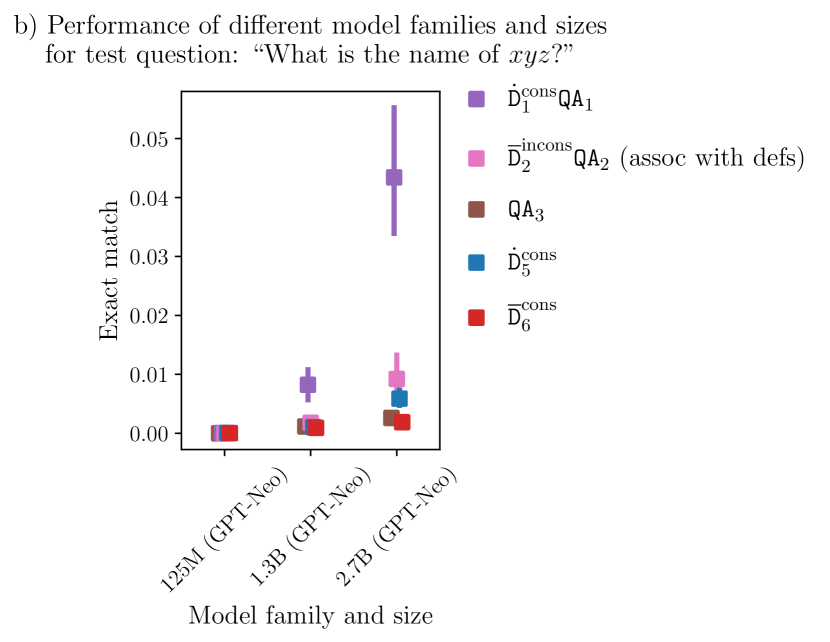
Figure 16: Performance of GPT-Neo models of different sizes trained on the harder T-REx-based dataset. We observe both OCL and meta-OCL only with the largest GPT-Neo model. a) We plot the performance for $\dot{\mathtt{D}}_{1}^{\text{cons}}\mathtt{QA}_{1}$ and $\bar{\mathtt{D}}_{2}^{\text{incons}}\mathtt{QA}_{2}$ after the first finetuning stage, and for $\dot{\mathtt{D}}_{5}^{\text{cons}}$ and $\bar{\mathtt{D}}_{6}^{\text{cons}}$ after the second stage. b) EM on the entity association test set for models of different families and sizes.

C.6 Sequence-to-sequence model experiments: setup and results

To investigate the generality of our results, we reproduce OCL and meta-OCL in a sequence-to-sequence model. We employ T5-3B (Raffel et al.,, 2020), an encoder-decoder transformer, where the loss is calculated only for the outputs of the decoder that produces the answer. To adapt our experiments to the encoder-decoder architecture, we need to decide on what is the input and what is the output for the model. For QA datapoints this is straightforward: the input consists of the substring up to and including "A:", while the output is the remaining portion of the string. For example, the QA string “Q: what did xyz do? A: Queen” gets divided into “Q: what did xyz do? A:” and “ Queen”. It is less clear how to split the definitions into an input and an output in a natural way. We settle on splitting them similarly to QA datapoints: “  xyz Cleopatra” is split into “  xyz” (input) and “ Cleopatra” (output). Our results for single-stage and two-stage finetuning are shown in Figures 17 and 18.

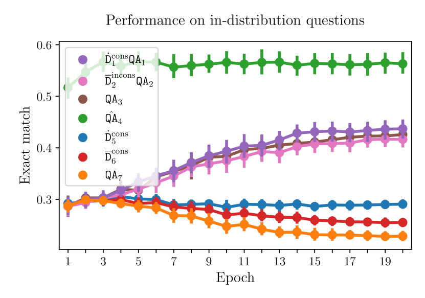
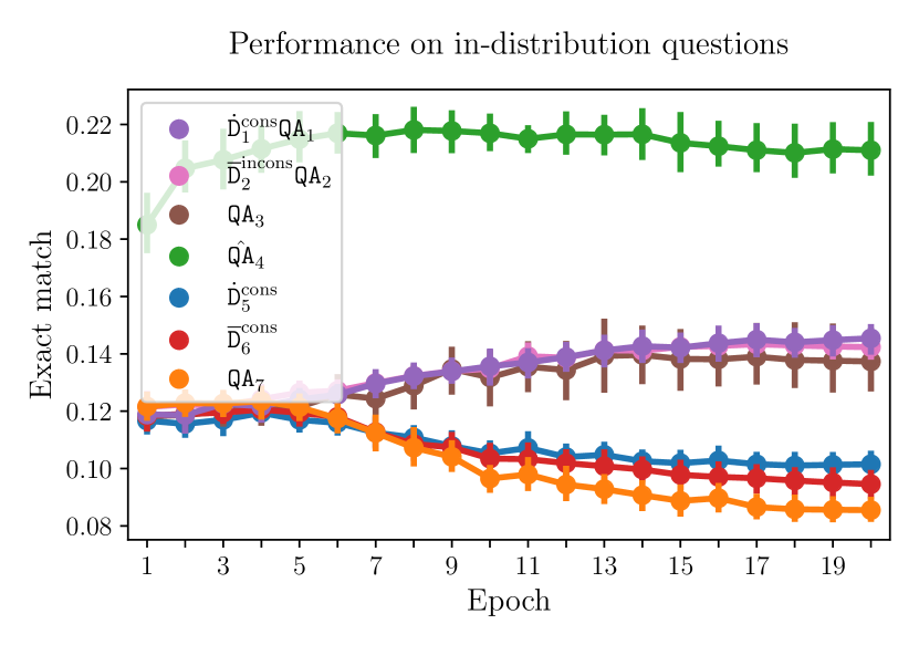
Figure 17: T5-3B finetuned in a single stage on CVDB (left) and T-REx (right) datasets over 10 seeds. The OCL effect is present but barely visible; a meta-OCL-like effect is seemingly present, but it is not clear what is actually going on, as the accuracy is going down.

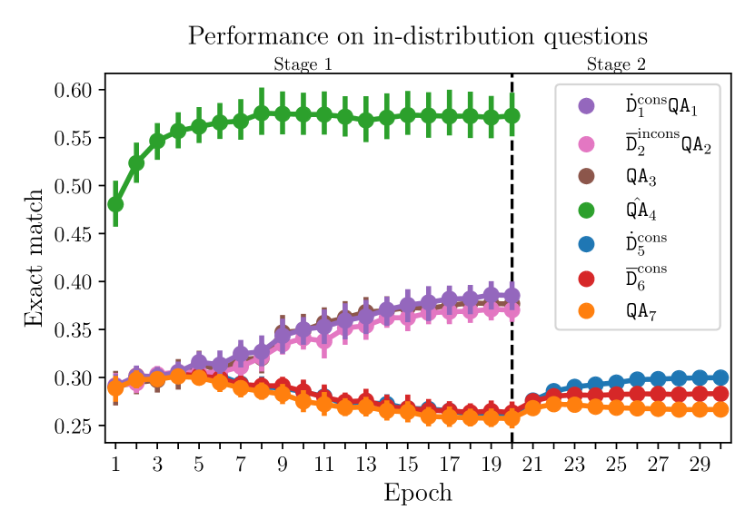
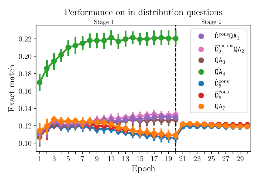
Figure 18: T5-3B finetuned in two stages on CVDB (left) and T-REx (right) datasets. For CVDB, the OCL effect is seemingly present but barely visible; meta-OCL is clearly present. For T-REx, looks like neither OCL nor meta-OCL is present.

Appendix D Set inclusion experiment

Data setup.

Data splits are produced similarly to those in the QA experiment (Sec. A.3), and are summarized in Table 3. We generate test questions such that half of them have the correct answer "Yes" and half "No", hence random guessing would result in 50% accuracy.

	Subset	Percent variables
$\mathcal{X}_{1}$	$\dot{\mathtt{D}}_{1}^{\text{cons}}\mathtt{QA}_{1}$	0.4
	$\bar{\mathtt{D}}_{2}^{\text{incons}}\mathtt{QA}_{2}$	0.4
$\mathcal{X}_{2}$	$\dot{\mathtt{D}}_{5}^{\text{cons}}$	0.1
	$\bar{\mathtt{D}}_{6}^{\text{cons}}$	0.1

Table 3: Fraction of the 8000 variables assigned to each data subset.

Hyperparameters

We use the Adafactor optimizer (Shazeer and Stern,, 2018) with the batch size of 512 datapoints; all the other hyperparameters are Pythia-70m defaults. We train the model from scratch for 100 epochs in the first stage, and for 40 epochs in the second stage.

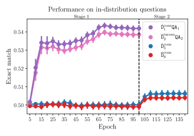
Figure 19: Set inclusion experiment, Pythia-70M model with a custom tokenizer trained from scratch over 50 seeds. We observe both OCL and meta-OCL. An interesting aspect of this experiment is that if we increase the number of training questions in $\mathcal{X}_{1}$ per each variable (currently 12), we get much better performance on the validation questions, but the consistent definitions stop making a difference.

Appendix E MNIST experiment

E.1 MNIST QA Dataset

Here, we give the implementation details for the MNIST dataset, as described in Section 3.2. We used a $3\times 3$ grid variant of the dataset, yielding $10^{9}$ possible combinations of digits for the possible values of the variables.

For the training dataset, the digit images to be concatenated into a grid are sampled uniformly at random from all images with the adequate label from the MNIST train split. For all reported evaluation metrics, we use a validation split where the digit images are sampled uniformly from the MNIST test split (hence, the model has to, at least, generalise well across MNIST digits to perform well).

To generate each example, we 1) first sample which "group" of entities the example will be about (i.e. which of $(\dot{\mathtt{D}}_{1}^{\text{cons}}\mathtt{QA}_{1}),(\bar{\mathtt{D}}_{2}^{\text{incons}}\mathtt{QA}_{2}),(\mathtt{QA}_{3}),\dots$ in $\mathcal{X}_{1}\cup\mathcal{X}_{2}$, each with equal probability), 2) whether it will be a definition or a QA example (it’s a definition with probability $0.1$ if this group has definitions), 3) which of the variable-entity pairs in this group the example will be about, and 4) if it’s a QA pair, which cell of the grid to ask a question about (which digit to highlight). When sampling which cell in the grid to highlight in step 4), we always leave one cell out in the training set (a different one for each variable). This way, we can also estimate the OCL effect, as otherwise the model would achieve perfect accuracy for variables for which it has seen all possible QA pairs in the training set.

At each step of training, we sample a new batch of examples in this way, effectively giving us one-epoch training; in all likelihood, no two examples seen during training will be exactly alike.

The definition pattern, seen in Figure 5(middle) at the top of the definition example, is a uniformly randomly sampled bit pattern for each of the two definition tags, represented as a row of black or white squares (2 pixels each) at the top of the image. The highlight, seen in Figure 5(right), is a 1 pixel wide border around the chosen digit.

E.2 Hyperparameters for the MNIST QA experiments

For the MNIST QA experiments, we train a ConvNeXt V2 model (Woo et al.,, 2023), a variant of the ConvNeXt model proposed by Liu et al., (2022). We use the “Tiny” variant – a convolutional model with $28.6$ million parameters. We train the model with $\mathtt{AdamW}$ for $120000$ training steps with a batch-size of $128$, learning rate $3\times 10^{-4}$, $2000$ steps of linear learning rate warm-up, and other optimization hyperparameters matching the original paper.

E.3 OCL and meta-OCL results for the MNIST QA Dataset

Out-of-context learning.

As mentioned in Section 3.2, we observe OCL in the MNIST QA experiments. The results are shown in Figure 20 (left). As described in Section E, even for the entity groups $\dot{\mathtt{D}}_{1}^{\text{cons}}\mathtt{QA}_{1}$ and $\bar{\mathtt{D}}_{2}^{\text{incons}}\mathtt{QA}_{2}$ for which QA pairs were present in the training dataset, using definitions is required to get perfect accuracy on the test set, since we never ask questions about one of the grid cells for each variable in the training set. This makes OCL apparent in Figure 20 (left).

Meta-OCL.

As seen in Figure 20 (right), we also observe meta-OCL in this setting. Given a sufficient number (i.e. $\geq 50$) of variable-entity pairs, the model performs much better on QA pairs for variables defined using the definition tag that was consistent for other examples in the training set ($\dot{\mathtt{D}}_{5}^{\mathtt{cons}}$), compared to the tag that was inconsistent ($\overline{\mathtt{D}}_{6}^{\mathtt{cons}}$), with the effect increasing in the number of variable-entity pairs.

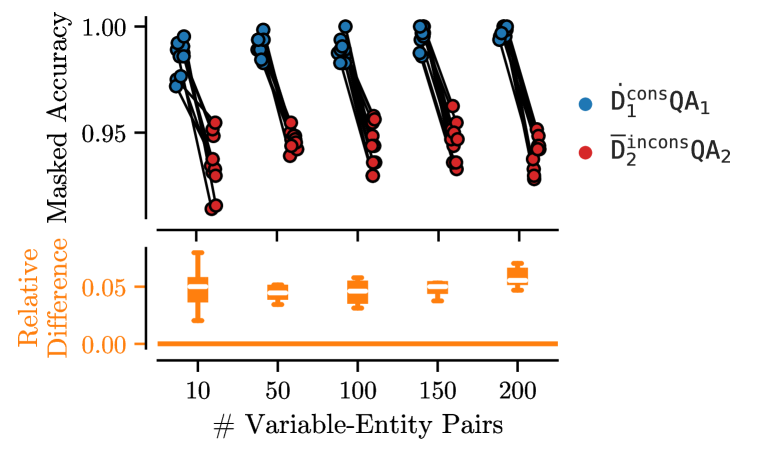
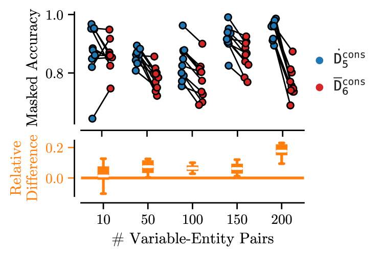
Figure 20: We observe both OCL (left) and meta-OCL (right) in the MNIST QA experiments.

Appendix F Computational resources used for our experiments

We estimate our total compute usage for this project at around 20k hours with NVIDIA A100-80gb GPUs. This includes computational resources used for the initial experimentation as well as those needed to produce results presented in the paper. Running a single seed of the two-stage CVDB experiment with the Pythia-2.8B model takes about 6 GPU hours. Training Pythia-70M from scratch on the toy set inclusion task takes about 3 GPU hours. Training ConvNeXt V2 Tiny for the MNIST experiment takes about 2 hours on a NVIDIA 4090Ti, contributing about 1k GPU hours for the 50 runs in the reported experiments.

References

- Andreas, (2022) Andreas, J. (2022). Language models as agent models. arXiv preprint arXiv:2212.01681.
- (2) Berglund, L., Stickland, A. C., Balesni, M., Kaufmann, M., Tong, M., Korbak, T., Kokotajlo, D., and Evans, O. (2023a). Taken out of context: On measuring situational awareness in llms. arXiv preprint arXiv:2309.00667.
- (3) Berglund, L., Tong, M., Kaufmann, M., Balesni, M., Stickland, A. C., Korbak, T., and Evans, O. (2023b). The reversal curse: Llms trained on" a is b" fail to learn" b is a". arXiv preprint arXiv:2309.12288.
- Biderman et al., (2023) Biderman, S., Schoelkopf, H., Anthony, Q., Bradley, H., O’Brien, K., Hallahan, E., Khan, M. A., Purohit, S., Prashanth, U. S., Raff, E., et al. (2023). Pythia: A suite for analyzing large language models across training and scaling. arXiv preprint arXiv:2304.01373.
- Black et al., (2021) Black, S., Gao, L., Wang, P., Leahy, C., and Biderman, S. (2021). GPT-Neo: Large Scale Autoregressive Language Modeling with Mesh-Tensorflow. If you use this software, please cite it using these metadata.
- Brown et al., (2020) Brown, T., Mann, B., Ryder, N., Subbiah, M., Kaplan, J. D., Dhariwal, P., Neelakantan, A., Shyam, P., Sastry, G., Askell, A., et al. (2020). Language models are few-shot learners. Advances in neural information processing systems, 33:1877–1901.
- Burns et al., (2022) Burns, C., Ye, H., Klein, D., and Steinhardt, J. (2022). Discovering latent knowledge in language models without supervision. arXiv preprint arXiv:2212.03827.
- Carroll et al., (2022) Carroll, M. D., Dragan, A., Russell, S., and Hadfield-Menell, D. (2022). Estimating and penalizing induced preference shifts in recommender systems. In International Conference on Machine Learning, pages 2686–2708. PMLR.
- Chan et al., (2022) Chan, S. C., Santoro, A., Lampinen, A. K., Wang, J. X., Singh, A., Richemond, P. H., McClelland, J., and Hill, F. (2022). Data distributional properties drive emergent few-shot learning in transformers. arXiv preprint arXiv:2205.05055.
- Cohen et al., (2022) Cohen, M., Hutter, M., and Osborne, M. (2022). Advanced artificial agents intervene in the provision of reward. AI Magazine, 43(3):282–293.
- Dandi et al., (2022) Dandi, Y., Barba, L., and Jaggi, M. (2022). Implicit gradient alignment in distributed and federated learning. In Proceedings of the AAAI Conference on Artificial Intelligence, volume 36, pages 6454–6462.
- Deng, (2012) Deng, L. (2012). The mnist database of handwritten digit images for machine learning research [best of the web]. IEEE signal processing magazine, 29(6):141–142.
- Elsahar et al., (2018) Elsahar, H., Vougiouklis, P., Remaci, A., Gravier, C., Hare, J., Laforest, F., and Simperl, E. (2018). T-rex: A large scale alignment of natural language with knowledge base triples. In Proceedings of the Eleventh International Conference on Language Resources and Evaluation (LREC 2018).
- Finn et al., (2017) Finn, C., Abbeel, P., and Levine, S. (2017). Model-agnostic meta-learning for fast adaptation of deep networks. In International conference on machine learning, pages 1126–1135. PMLR.
- Fort et al., (2019) Fort, S., Nowak, P. K., Jastrzebski, S., and Narayanan, S. (2019). Stiffness: A new perspective on generalization in neural networks. arXiv preprint arXiv:1901.09491.
- Gao et al., (2020) Gao, L., Biderman, S., Black, S., Golding, L., Hoppe, T., Foster, C., Phang, J., He, H., Thite, A., Nabeshima, N., et al. (2020). The pile: An 800gb dataset of diverse text for language modeling. arXiv preprint arXiv:2101.00027.
- Grosse et al., (2023) Grosse, R., Bae, J., Anil, C., Elhage, N., Tamkin, A., Tajdini, A., Steiner, B., Li, D., Durmus, E., Perez, E., et al. (2023). Studying large language model generalization with influence functions. arXiv preprint arXiv:2308.03296.
- Janus, (2022) Janus (2022). Simulators. Alignment Forum https://www.alignmentforum.org/posts/vJFdjigzmcXMhNTsx/simulators.
- Krueger et al., (2020) Krueger, D., Maharaj, T., and Leike, J. (2020). Hidden incentives for auto-induced distributional shift. arXiv preprint arXiv:2009.09153.
- Laouenan et al., (2022) Laouenan, M., Bhargava, P., Eyméoud, J.-B., Gergaud, O., Plique, G., and Wasmer, E. (2022). A cross-verified database of notable people, 3500bc-2018ad. Scientific Data, 9(1):1–19.
- Lee et al., (2021) Lee, S., Lee, H. B., Lee, J., and Hwang, S. J. (2021). Sequential reptile: Inter-task gradient alignment for multilingual learning. arXiv preprint arXiv:2110.02600.
- Levinstein and Soares, (2020) Levinstein, B. A. and Soares, N. (2020). Cheating death in damascus. The Journal of Philosophy, 117(5):237–266.
- Li et al., (2021) Li, B. Z., Nye, M., and Andreas, J. (2021). Implicit representations of meaning in neural language models. arXiv preprint arXiv:2106.00737.
- (24) Li, D., Rawat, A. S., Zaheer, M., Wang, X., Lukasik, M., Veit, A., Yu, F., and Kumar, S. (2022a). Large language models with controllable working memory. arXiv preprint arXiv:2211.05110.
- Li et al., (2018) Li, D., Yang, Y., Song, Y.-Z., and Hospedales, T. (2018). Learning to generalize: Meta-learning for domain generalization. In Proceedings of the AAAI conference on artificial intelligence, volume 32.
- (26) Li, K., Hopkins, A. K., Bau, D., Viégas, F., Pfister, H., and Wattenberg, M. (2022b). Emergent world representations: Exploring a sequence model trained on a synthetic task. arXiv preprint arXiv:2210.13382.
- Liu et al., (2022) Liu, Z., Mao, H., Wu, C.-Y., Feichtenhofer, C., Darrell, T., and Xie, S. (2022). A convnet for the 2020s. In Proceedings of the IEEE/CVF Conference on Computer Vision and Pattern Recognition, pages 11976–11986.
- Lu et al., (2021) Lu, Y., Bartolo, M., Moore, A., Riedel, S., and Stenetorp, P. (2021). Fantastically ordered prompts and where to find them: Overcoming few-shot prompt order sensitivity. arXiv preprint arXiv:2104.08786.
- Meng et al., (2022) Meng, K., Bau, D., Andonian, A., and Belinkov, Y. (2022). Locating and editing factual knowledge in gpt. arXiv preprint arXiv:2202.05262.
- Mitchell et al., (2021) Mitchell, E., Lin, C., Bosselut, A., Finn, C., and Manning, C. D. (2021). Fast model editing at scale. arXiv preprint arXiv:2110.11309.
- Mitchell and Krakauer, (2023) Mitchell, M. and Krakauer, D. C. (2023). The debate over understanding in ai’s large language models. Proceedings of the National Academy of Sciences, 120(13):e2215907120.
- Ngo, (2022) Ngo, R. (2022). The alignment problem from a deep learning perspective. arXiv preprint arXiv:2209.00626.
- Nichol et al., (2018) Nichol, A., Achiam, J., and Schulman, J. (2018). On first-order meta-learning algorithms. arXiv preprint arXiv:1803.02999.
- Olah et al., (2020) Olah, C., Cammarata, N., Schubert, L., Goh, G., Petrov, M., and Carter, S. (2020). Zoom in: An introduction to circuits. Distill, 5(3):e00024–001.
- Parascandolo et al., (2020) Parascandolo, G., Neitz, A., Orvieto, A., Gresele, L., and Schölkopf, B. (2020). Learning explanations that are hard to vary. arXiv preprint arXiv:2009.00329.
- Petroni et al., (2019) Petroni, F., Rocktäschel, T., Lewis, P., Bakhtin, A., Wu, Y., Miller, A. H., and Riedel, S. (2019). Language models as knowledge bases? arXiv preprint arXiv:1909.01066.
- Raffel et al., (2020) Raffel, C., Shazeer, N., Roberts, A., Lee, K., Narang, S., Matena, M., Zhou, Y., Li, W., and Liu, P. J. (2020). Exploring the limits of transfer learning with a unified text-to-text transformer. The Journal of Machine Learning Research, 21(1):5485–5551.
- Roberts, (2021) Roberts, D. A. (2021). Sgd implicitly regularizes generalization error. arXiv preprint arXiv:2104.04874.
- Shazeer and Stern, (2018) Shazeer, N. and Stern, M. (2018). Adafactor: Adaptive learning rates with sublinear memory cost. In International Conference on Machine Learning, pages 4596–4604. PMLR.
- Shi et al., (2021) Shi, Y., Seely, J., Torr, P. H., Siddharth, N., Hannun, A., Usunier, N., and Synnaeve, G. (2021). Gradient matching for domain generalization. arXiv preprint arXiv:2104.09937.
- Sinitsin et al., (2020) Sinitsin, A., Plokhotnyuk, V., Pyrkin, D., Popov, S., and Babenko, A. (2020). Editable neural networks. arXiv preprint arXiv:2004.00345.
- Smith et al., (2021) Smith, S. L., Dherin, B., Barrett, D. G., and De, S. (2021). On the origin of implicit regularization in stochastic gradient descent. arXiv preprint arXiv:2101.12176.
- Touvron et al., (2023) Touvron, H., Martin, L., Stone, K., Albert, P., Almahairi, A., Babaei, Y., Bashlykov, N., Batra, S., Bhargava, P., Bhosale, S., et al. (2023). Llama 2: Open foundation and fine-tuned chat models. arXiv preprint arXiv:2307.09288.
- Wolf et al., (2020) Wolf, T., Debut, L., Sanh, V., Chaumond, J., Delangue, C., Moi, A., Cistac, P., Rault, T., Louf, R., Funtowicz, M., et al. (2020). Transformers: State-of-the-art natural language processing. In Proceedings of the 2020 conference on empirical methods in natural language processing: system demonstrations, pages 38–45.
- Woo et al., (2023) Woo, S., Debnath, S., Hu, R., Chen, X., Liu, Z., Kweon, I. S., and Xie, S. (2023). Convnext v2: Co-designing and scaling convnets with masked autoencoders. arXiv preprint arXiv:2301.00808.
- Xie et al., (2021) Xie, S. M., Raghunathan, A., Liang, P., and Ma, T. (2021). An explanation of in-context learning as implicit bayesian inference. arXiv preprint arXiv:2111.02080.
- Zhang et al., (2019) Zhang, M., Lucas, J., Ba, J., and Hinton, G. E. (2019). Lookahead optimizer: k steps forward, 1 step back. Advances in neural information processing systems, 32.
- Zhao et al., (2021) Zhao, Z., Wallace, E., Feng, S., Klein, D., and Singh, S. (2021). Calibrate before use: Improving few-shot performance of language models. In International Conference on Machine Learning, pages 12697–12706. PMLR.