Relative Equilibria of Mechanical Systems with Rotational Symmetry

Abstract

We consider the task of classifying relative equilibria for mechanical systems with rotational symmetry. We divide relative equilibria into two natural groups: a generic class which we call normal, and a non-generic abnormal class. The eigenvalues of the locked inertia tensor descend to shape-space and endow it with the geometric structure of a 3-web with the property that any normal relative equilibrium occurs as a critical point of the potential restricted to a leaf from the web. To demonstrate the utility of this web structure we show how the spherical 3-body problem gives rise to a web of Cayley cubics on the 3-sphere, and use this to fully classify the relative equilibria for the case of equal masses.

Background and Outline

Finding general solutions of a dynamical system is often far too much to ask. Instead, we redirect our efforts to finding ‘special’ solutions which are more tractable. The equilibria are one such example. There is another example if the system admits a symmetric group action by a Lie group $G$, namely the relative equilibria (RE). These are solutions which are themselves orbits of one-parameter subgroups of $G$.

Perhaps the most famous examples of RE are the central configurations in the planar $n$-body problem. These are solutions where the bodies rotate around their centre of mass as if they were a rigid system. They were classified for $n=3$ by Euler and Lagrange, but for general $n$ only partial results are known. Even the question of whether there exist finitely many RE for $n>5$ remains unsolved (Problem 6 in Smale’s list [22]).

To motivate the results of this paper it is worth taking a quick look at what is involved in finding RE for the $n$-body problem with equal masses. Let $q$ be the vector of particle positions and $F$ the vector of forces. The centrifugal force scales linearly with distance, and so to balance the forces in a rotating frame we require

$$F=-\kappa q$$

for some positive $\kappa$. Force is the negative gradient of the potential $V$ and the vector $q$ is half the gradient of the inertia $\lambda=|q|^{2}$. Thus, we have a Lagrange-multiplier problem $2\nabla V=\kappa\nabla\lambda$. Since the inertia and potential are rotationally symmetric, we may as well take the quotient of all configurations with a common centre of mass by $\mathbf{SO}(2)$ to obtain what is called the shape space. Classifying RE now amounts to finding critical points of the potential restricted to level sets of the inertia in shape space.

There is a very nice picture of this for the 3-body problem. The level sets of the inertia in shape space are pairs-of-pants, as shown in Figure 1 (see [17, Ch. 14] for a good explanation). One can directly see the RE as the critical points of the potential: the Euler solutions are the three saddle points around the equator, and the two critical points on the top and bottom are the Lagrangian solutions.

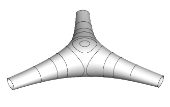
Figure 1: Constant inertia surface in shape space for the planar 3-body problem. The contours are of the potential energy.

The impetus for this work came from asking whether there is a similar nice picture for the spherical 3-body problem, where the bodies are now constrained to move on a sphere. This problem has attracted growing interest in the last few years (we recommend [2] for a good review of the literature). Unlike the planar problem, there is no such thing as a centre-of-mass frame, and so one must consider the larger group $\mathbf{SO}(3)$ of rotations. This means that it no longer makes sense to talk about the inertia in shape space, since the inertia now depends not just on the shape of the bodies but also on the axis of rotation. However, the eigenvalues of the inertia tensor do descend to shape space, and their level sets define a geometric structure which we call a web.

Definition 1.

A k-web on a manifold is a collection of regular foliations $\{\mathcal{F}_{1},\dots,\mathcal{F}_{k}\}$ defined almost everywhere and given locally by the level sets of functions $\Lambda_{1},\dots,\Lambda_{k}$.

We can now state our main result. Let $Q$ be a configuration space upon which $\mathbf{SO}(3)$ acts freely, and equip it with a potential energy $V$ which is invariant with respect to the action.

Theorem 1.

The eigenvalues of the locked inertia tensor $\mathbb{I}_{q}$ descend to shape space $\mathcal{B}=Q/\mathbf{SO}(3)$ and their level sets endow it with the structure of a 3-web. A point $x$ in $\mathcal{B}$ is a normal relative equilibrium if and only if $2\nabla{V}=\kappa\nabla\lambda_{j}$ for some multiplicity-1 eigenvalue $\lambda_{j}$ and some $\kappa\geq 0$. In particular, $x$ must be a critical point of ${V}$ restricted to the leaf of constant $\lambda_{j}$. The angular momentum of the relative equilibrium is an eigenvector $L_{j}$ of $\mathbb{I}_{q}$ with eigenvalue $\lambda_{j}$ and magnitude $|L_{j}|^{2}=\kappa\lambda_{j}^{2}$.

In the context of the theorem a normal RE is understood to mean a RE whose angular momentum is not an eigenvector of the inertia tensor for a repeated eigenvalue. The abnormal RE are quite special, since it is precisely where the eigenvalues are repeated that the 3-web becomes singular. Classifying the abnormal RE requires a separate analysis, and are possibly related to the presence of degenerate RE which are not ‘persistent’ in phase space (in the sense described in [15]).

To frame how Theorem 1 compares with existing methods of classifying RE some historical comments are in order. Let $M$ be a symplectic manifold equipped with a Hamiltonian group action $G$ with momentum map $\Phi$. In his study of the planar $n$-body problem, Smale devises an effective characterisation of the RE as critical points of the energy-momentum map [20, 21]. Thus, if $H$ is a $G$-invariant Hamiltonian on $M$, the RE are classified by the critical points of $H$ restricted to a level set $\Phi^{-1}(\mu)$. Equivalently, one talks of critical points of the augmented Hamiltonian $H_{\mu}=H-\langle\Phi,\mu\rangle$.

We can go one step further by passing to the quotient and considering critical points of the reduced Hamiltonian on the symplectic reduced space $\Phi^{-1}(\mu)/G_{\mu}$. Thus, for a mechanical system $M=T^{*}Q$ we have the task of classifying critical points on a manifold of dimension

$$2\dim Q-\dim G-\dim G_{\mu}.$$

In particular, for the case of rotational symmetry where $G=\textbf{SO}(3)$, this will typically involve finding critical points on a manifold of dimension $2\dim Q-4$.

In fact, for mechanical systems we can improve upon this still by considering the amended potential

$$V_{\mu}(q)=V(q)+\frac{1}{2}\langle\mu,\mathbb{I}_{q}^{-1}(\mu)\rangle.$$

The RE of a mechanical system can equivalently be characterised as critical points of $V_{\mu}$ [14]. From a computational perspective this is a significant improvement, since we need only compute critical points on a manifold of dimension $\dim Q$. However, how should one choose $\mu$ in the amended potential? The magnitude of $\mu$ clearly makes a difference, however choosing a different $\operatorname{Ad}_{g}^{*}\mu$ on the coadjoint orbit through $\mu$ shouldn’t make much difference, since both the dynamics and momentum map are $G$-equivariant.

Theorem 1 can be seen as a way of eliminating this redundancy in the choice of $\mu$. The amended potential does not descend to shape space. However, by locally describing the configuration space as a principal (left) $G$-bundle over shape space, we can introduce a slightly different notion of amended potential $V_{L}$ which is defined with respect to the ‘body’ momentum $L$ (as opposed to the ‘spatial’ momentum $\mu$). This function does descend to shape space, and is a crucial step in establishing the theorem.

In summary, this theorem furnishes shape space with additional geometric structure, and provides a less taxing method for classifying the RE. Indeed, RE can now be classified as critical points restricted to a leaf of the web, which will typically have dimension $\dim Q-4$; an improvement over the amended potential method. In answer to our original question, we do indeed find a nice picture for the spherical 3-body problem, and we invite the reader to skip ahead to Figure 4 to behold a 3-web of Cayley cubics in shape space.

We conclude with a brief outline of the paper. In Section 1 we prove a stronger version of Theorem 1 which applies to any compact group acting freely on configuration space. Section 2 presents a trio of 3-webs arising from physical problems: the compressible liquid drop, the triatomic molecule, and the full-body satellite problem. We show how an understanding of these webs can be used to derive various existence results for RE. In Section 3 we apply Theorem 1 to obtain a complete and self-contained classification of the RE for the equal-mass spherical 3-body problem. We would like to point out that this classification is not new, having recently been established in a series of preprints by Fujiwara & Pérez-Chavela [9, 10, 8, 12, 11, 13]. In the final section we discuss the generalisation of the web formalism to mechanical systems with larger symmetry groups. For the famous example of the Dirichlet system [6] we show how a one-parameter family of 6-webs arises on shape space, and use this to classify a family of Riemann ellipsoids.

1 Main Result

Let $Q$ be configuration space and $G$ a Lie group which acts on $Q$. We shall suppose that the orbit-map $\pi\colon Q\rightarrow\mathcal{B}$ is a smooth principal $G$-bundle onto the shape space $\mathcal{B}=Q/G$. We note that this assumption automatically holds if the action is free and the group compact. Additionally, we equip $Q$ with a $G$-invariant metric, and a $G$-invariant scalar function $V$.

1.1 Equations of Motion

The horizontal subspace $H_{q}$ is the orthogonal complement to the tangent space of the $G$-orbit passing through $q\in Q$. The pushforward of $\pi$ establishes an isomorphism between $H_{q}$ and the tangent space to $x=\pi(q)$. Since the metric on $Q$ is $G$-invariant, the pushforward-metric does not depend on the choice of $q$ in the fibre of $\pi$, and hence, we have a well-defined reduced metric on $\mathcal{B}$.

Let $U$ be a chart of $\mathcal{B}$ and $\sigma$ a local section of the bundle over $U$. Consider the decomposition of a tangent vector into its horizontal and vertical parts $\dot{q}=H+V$. We may identify this with the pair $\dot{x}=\pi_{*}(H)$ and $\dot{g}$, where $V=\dot{g}\sigma(x)$. This establishes an orthogonal decomposition $T_{U}Q=TU\times TG$. As the metric is $G$-invariant, the length of a vertical vector $\dot{g}q$ is the same as $\omega q$, where $\omega=g^{-1}\dot{g}$ is the angular velocity in the Lie algebra $\mathfrak{g}$. It follows that

$$|\dot{q}|^{2}=\langle\mathbb{M}_{x}(\dot{x}),\dot{x}\rangle+\langle\mathbb{I}_{\sigma(x)}(\omega),\omega\rangle$$ (1.1)

where $\mathbb{M}_{x}\colon T_{x}B\rightarrow T_{x}^{*}B$ is the metric tensor for the reduced metric on shape space, and $\mathbb{I}_{q}\colon\mathfrak{g}\rightarrow\mathfrak{g}^{*}$ is the symmetric (locked) inertia tensor satisfying $|\omega q|^{2}=\langle\mathbb{I}_{q}(\omega),\omega\rangle$ for all $\omega$.

Remark 1.1.

If we choose a different section $\sigma\mapsto g\sigma$ then the inertia tensor varies according to the representation of $G$ on $\text{Sym}^{2}\mathfrak{g}^{*}$ given by

$$\mathbb{I}_{gq}=\operatorname{Ad}_{g}^{*}\circ~{}\mathbb{I}_{q}\circ\operatorname{Ad}_{g}^{-1}.$$ (1.2)

We now consider a mechanical system on $Q$ with Lagrangian $|\dot{q}|^{2}/2-V(q)$. The Legendre transform on $T_{U}Q=TU\times TG$ sends the tangent vector $(\dot{x},g\omega)$ to $(y,gL)$ where

$$y=\mathbb{M}_{x}(\dot{x})$$

is the reduced momentum in $T^{*}_{x}B$, and

$$L=\mathbb{I}_{\sigma(x)}(\omega)$$

is the angular momentum in $\mathfrak{g}^{*}$. The Hamiltonian on $T^{*}U\times T^{*}G$ is thus,

$$H(x,y;g,L)=\frac{1}{2}\langle y,\mathbb{M}_{x}^{-1}(y)\rangle+\frac{1}{2}\langle L,\mathbb{I}_{\sigma(x)}^{-1}(L)\rangle+{V}(x).$$ (1.3)

In a slight abuse of notation we also write $V$ to mean the reduced potential on $\mathcal{B}$. Observe that this Hamiltonian does not depend on $g$. Indeed, it descends to a Hamiltonian system on the Poisson-reduced space $T^{*}U\times\mathfrak{g}^{*}$ given by left-translating covectors on $T^{*}G$ to $\mathfrak{g}^{*}$. The Poisson structure is the product of the standard structures on $T^{*}U$ and $\mathfrak{g}^{*}$, and hence, we may write the reduced equations of motion

$$\dot{x} =\mathbb{M}_{x}^{-1}(y),$$ (1.4)

$$\dot{y} =-\frac{1}{2}\nabla\left(\langle y,\mathbb{M}_{x}^{-1}y\rangle+\langle L,\mathbb{I}_{x}^{-1}L\rangle\right)-\nabla V,$$ (1.5)

$$\dot{L} =\operatorname{ad}_{\omega}^{*}L.$$ (1.6)

In these equations we are now writing $\mathbb{I}_{x}$ instead of $\mathbb{I}_{\sigma(x)}$ (the dependence on the choice of section $\sigma$ will now be implicit).

Remark 1.2.

The momentum map on $T^{*}U\times T^{*}G$ generating the left-action of $G$ is given by right-translating covectors on $T^{*}G$ to $\mathfrak{g}^{*}$. Thus, we have that $\mu=\Phi(gL)=Ad_{g}^{*}L$ is a conserved quantity $\mu\in\mathfrak{g}$. In analogy with rigid body dynamics, we can think of $L$ and $\mu$ as being the ‘body’ and ‘spatial’ angular momentum, respectively.

1.2 Theorem

A RE is a solution contained to a group orbit. Hence, RE correspond to fixed points $(x_{0},y_{0},L_{0})$ of the reduced equations of motion in $T^{*}U\times\mathfrak{g}^{*}$. Clearly, from Eq. (1.4) we require $y_{0}=0$, and so when we talk of RE we shall only make reference to the $(x_{0},L_{0})$-coordinate. The pair $(x_{0},L_{0})$ is a RE if and only if

$$\frac{1}{2}\nabla\big{|}_{x_{0}}\langle L_{0},\mathbb{I}_{x}^{-1}L_{0}\rangle=-\nabla V\big{|}_{x_{0}},$$ (1.7)

$$\operatorname{ad}_{\omega}^{*}L_{0}=0.$$ (1.8)

A necessary condition for $(x_{0},L_{0})$ to be a RE is that $x_{0}$ be a critical point of the (reduced) amended potential

$$V_{L}(x)=V(x)+\frac{1}{2}\langle L_{0},\mathbb{I}_{x}^{-1}L_{0}\rangle.$$ (1.9)

However, this is not sufficient, since we also require that Eq. (1.8) be satisfied.

Lemma 1.1.

A necessary condition for $(x_{0},L_{0})$ to be a relative equilibrium is that $L_{0}$ be a critical point of the quadratic function $\langle L,\mathbb{I}_{x_{0}}^{-1}L\rangle$ restricted to the coadjoint orbit $\mathcal{O}$ through $L_{0}$.

Proof.

Fix an $x$ and consider the function $\langle L,\mathbb{I}_{x}^{-1}L\rangle$ on $\mathfrak{g}^{*}$. The infinitesimal change in this function generated by moving along a tangent vector $\operatorname{ad}_{\xi}^{*}L$ is

$$\langle\operatorname{ad}_{\xi}^{*}L,\mathbb{I}_{x}^{-1}L\rangle+\langle L,\mathbb{I}_{x}^{-1}\operatorname{ad}_{\xi}^{*}L\rangle.$$

Since the inertia tensor is symmetric, and writing $\omega=\mathbb{I}_{x}^{-1}L$, we see that this is

$$2\langle\operatorname{ad}_{\xi}^{*}L,\omega\rangle=-2\langle\operatorname{ad}_{\omega}^{*}L,\xi\rangle.$$

Therefore, $L$ is a critical point of the function restricted to the coadjoint orbit if and only if this expression vanishes for all $\xi$, and hence, $\operatorname{ad}_{\omega}^{*}L=0$. ∎

Definition 2.

We will call a relative equilibrium $(x_{0},L_{0})$ normal if $L_{0}$ is a non-degenerate critical point of the function $\langle L,\mathbb{I}_{x_{0}}^{-1}L\rangle$ restricted to the coadjoint orbit $\mathcal{O}$ through $L_{0}$. Otherwise, we call the relative equilibrium abnormal.

Theorem 2.

Let $G$ be a compact Lie group acting freely and isometrically on a configuration space $Q$. For every coadjoint orbit $\mathcal{O}$ in $\mathfrak{g}^{*}$ the shape space $\mathcal{B}=Q/G$ inherits the structure of a web $\mathcal{W}_{\mathcal{O}}$ defined locally around every point by the level sets of functions $\Lambda_{0},\dots,\Lambda_{k}$. A point $x_{0}$ is a normal relative equilibrium with angular momentum belonging to a scalar multiple of $\mathcal{O}$ if and only if $-\nabla V=\kappa\nabla\Lambda_{j}$ for some $j$ and some $\kappa\geq 0$. In particular, $x_{0}$ must be a critical point of the potential restricted to a leaf of constant $\Lambda_{j}$.

Proof.

As the coadjoint orbit $\mathcal{O}$ is compact it must contain finitely many non-degenerate critical points $L_{0},\dots,L_{k}$ of the function $L\mapsto\langle L,\mathbb{I}_{x_{0}}^{-1}L\rangle$. Non-degenerate critical points are stable under perturbations, and so locally in some neighbourhood $U$ of $x_{0}$ we have $L_{j}(x)$ for $j=0,1,\dots,k$ with $L_{j}(x_{0})=L_{j}$ and which are non-degenerate critical points of $\langle L,\mathbb{I}_{x}^{-1}L\rangle$ restricted to $\mathcal{O}$ for each $x\in U$.

Introduce the functions $\Lambda_{j}(x)=\langle L_{j}(x),\mathbb{I}_{x}^{-1}L_{j}(x)\rangle$. We now make an explicit choice of section $\sigma$, choosing instead the section $g(x)\sigma(x)$ where $g(x)$ satisfies

$$\operatorname{Ad}^{*}_{g(x)}L_{0}(x)=L_{0}.$$

In light of Remark 1.1 we see that this choice of section has the effect of ensuring that

$$\Lambda_{0}(x)=\langle L_{0},\mathbb{I}_{x}^{-1}L_{0}\rangle$$

(where $\mathbb{I}_{x}$ now denotes the inertia tensor with respect to the new section). It follows that Eq. (1.7) is satisfied by $(x_{0},L_{0})$ if and only if

$$\frac{1}{2}\nabla\Lambda_{0}\Big{|}_{x_{0}}=-\nabla V\big{|}_{x_{0}}$$ (1.10)

The term on the left hand side is quadratic in $L_{0}$, and therefore, if $\nabla\Lambda_{0}$ is a negative scalar multiple of $\nabla V$, then there exists a scalar multiple $\alpha$ of $L_{0}$ satisfying Eq. (1.10). Specifically, $\alpha$ satisfies $\alpha^{2}|\nabla\Lambda_{0}|=2|\nabla V|^{2}$. ∎

1.3 The Special Case of Rotational Symmetry

For $G$ compact we may identify $\mathfrak{g}$ with its dual, and the adjoint representation with the coadjoint representation. The inertia tensor is now identified with a symmetric map $\mathbb{I}_{x}\colon\mathfrak{g}\rightarrow\mathfrak{g}$ and Eq. (1.8) becomes

$$[\omega,L]=0$$ (1.11)

where $[~{},~{}]$ denotes the Lie bracket on $\mathfrak{g}$. In particular, a necessary condition for $(x,L)$ to be a RE is that $\omega=\mathbb{I}_{x}^{-1}L$ be contained to the centralizer of $L$.

Proof of Theorem 1.

For the Lie algebra $\mathfrak{so}(3)$ the centralizer of any non-zero $L$ is the line spanned by $L$. Therefore, in the special case where $\mathfrak{g}=\mathfrak{so}(3)$ the solutions to Eq. (1.11) are the eigenvectors of $\mathbb{I}_{x}$. Observe that a RE with angular momentum $L$ is normal if and only if the corresponding eigenvalue has multiplicity one

The coadjoint orbits of $\mathfrak{so}(3)$ are spheres of constant $|L|^{2}$, and so all non-zero coadjoint orbits are scalar multiples of each other. If we now apply Theorem 2 to this special case then we see that the web is defined by the functions

$$\Lambda_{j}=\frac{|L_{j}|^{2}}{\lambda_{j}}$$

where $L_{j}$ is an eigenvector of $\mathbb{I}_{x}$ with eigenvalue $\lambda_{j}(x)$. Theorem 1 now follows by noting that $\nabla\Lambda_{j}=-|L_{j}|^{2}\lambda_{j}^{-2}\nabla\lambda_{j}$. ∎

Example 1.1 (The spherical 2-body problem).

Consider two non-colinear particles $q_{1}$ and $q_{2}$ on the unit sphere with masses $m_{1}$ and $m_{2}$, respectively. Suppose that they are subject to a strictly attractive potential force which only depends on the angle $\theta\in(0,\pi)$ subtended between them. The orbit-map $\pi:(\mathbf{S}^{2}\times\mathbf{S}^{2})\setminus\Delta\rightarrow(0,\pi)$ is a principal $\mathbf{SO}(3)$-bundle and admits a global section $\sigma$ sending $\theta$ to the pair $q_{1}=(1,0,0)$ and $q_{2}=(\cos\theta,\sin\theta,0)$. The locked inertia tensor for this pair of points is

$$\mathbb{I}_{\theta}=\begin{pmatrix}m_{2}\sin^{2}\theta&-\frac{m_{2}}{2}\sin 2\theta&0\\ -\frac{m_{2}}{2}\sin 2\theta&m_{1}+m_{2}\cos^{2}\theta&0\\ 0&0&m_{1}+m_{2}\end{pmatrix}$$ (1.12)

with characteristic polynomial

$$(m_{1}+m_{2}-t)\left(2t-m_{1}-m_{2}-\sqrt{D_{\theta}}\right)\left(2t-m_{1}-m_{2}+\sqrt{D_{\theta}}\right),$$ (1.13)

where $D_{\theta}=m_{1}^{2}+2m_{1}m_{2}\cos 2\theta+m_{2}^{2}$. The eigenvalue $\lambda_{0}=m_{1}+m_{2}$ is constant in $\theta$, and therefore defines a trivial leaf of the web equal to the whole of shape space. The two remaining eigenvalues

$$\lambda_{\pm}=\frac{m_{1}+m_{2}\pm\sqrt{D_{\theta}}}{2}$$

define leaves of the web which are discrete points. The derivatives $d\lambda_{\pm}/d\theta=\mp m_{1}m_{2}\sin 2\theta/\sqrt{D_{\theta}}$ have opposite signs, and hence, for a strictly attractive force with $dV/d\theta>0$, there exists a single normal RE (up to time-reversal symmetry) for every $\theta$, with inertia $\lambda_{+}$.

Remark 1.3.

To handle abnormal RE we must first identify the subset of shape space for which the inertia tensor admits repeated eigenvalues. Once we have done so, we must solve Eq. (1.7) but for when $L_{0}$ ranges over the whole eigenspace with the given eigenvalue.

For instance, in the previous example the inertia $\mathbb{I}_{\theta}$ only admits repeated eigenvalues when $m_{1}=m_{2}=m$ and for $\theta=\pi/2$. In this case, the eigenspace for the repeated eigenvalue is the plane $L_{0}=(u,v,0)$ with $u,v\in\mathbf{R}$. A computation reveals

$$\frac{d}{d\theta}\Big{|}_{\theta=\pi/2}\langle L_{0},\mathbb{I}_{\theta}^{-1}L_{0}\rangle=-2uv/m,$$ (1.14)

from which we conclude that an entire family of abnormal RE exist for the precise case of equal masses and $\theta=\pi/2$, provided $2uv=m|V(\pi/2)|$.

Incidentally, this remark together with the previous example fully classifies the RE for the spherical 2-body problem [1].

2 Examples of 3-Webs

The most interesting examples of 3-webs are those which we can visualise in 3-dimensional space. We should therefore like to gather examples of 6-dimensional configuration spaces $Q$ upon which $\mathbf{SO}(3)$ acts freely. Below we enumerate four examples together with a physical motivation for each.

$$\begin{array}[]{l|l|l}Q&\mathcal{B}&\text{Physical example}\\ \hline\cr\text{Sym}^{2}\mathbf{R}^{3}&\mathbf{R}^{3}_{\geq 0}/\mathbf{S}_{3}&\text{a compressible liquid drop}\\ \mathbf{R}^{3}\times\mathbf{R}^{3}&\text{a solid cone}&\text{a triatomic molecule}\\ \mathbf{SE}(3)&\mathbf{R}^{3}&\text{a body in a central force field }\\ \mathbf{S}^{2}\times\mathbf{S}^{2}\times\mathbf{S}^{2}&\mathbf{S}^{3}&\text{the spherical $3$-body problem}\end{array}$$

In this section we shall exhibit the 3-webs in the first three examples, following a common template, and presenting them in increasing order of complexity: for the liquid drop the web is given by linear planes, for the triatomic molecule they are planes and quadratic cones, and for the orbital satellite they are an intriguing family of quartic surfaces.

2.1 The Compressible Liquid Drop

Consider a liquid drop in $\mathbf{R}^{3}$ which at time $t=0$ is in some spherically-symmetric initial configuration. We shall model the motion of the liquid by supposing that at time $t$ the particle initially at $x_{0}$ is now at $S(t)x_{0}$, where $S$ is a symmetric matrix. The kinetic energy is given by

$$\frac{1}{2}\int|\dot{S}x_{0}|^{2}~{}dx_{0}=\frac{1}{2}\operatorname{Tr}(\dot{S}^{T}\dot{S})$$

where we have assumed that $\int x_{0}x_{0}^{T}dx_{0}=\text{Id}$. This defines a metric on the configuration space $\text{Sym}^{2}\mathbf{R}^{3}$ which is invariant with respect to conjugation by $\mathbf{O}(3)$. The orbit map $\pi\colon\text{Sym}^{2}\mathbf{R}^{3}\rightarrow\mathbf{R}^{3}_{\geq 0}/\mathbf{S}_{3}$ for this action sends $S$ to its eigenvalues $(x_{1},x_{2},x_{3})$ modulo permutations.

Remark 2.1.

We note that this shape space is not a smooth manifold, nor is the action of $\mathbf{O}(3)$ on $\text{Sym}^{2}\mathbf{R}^{3}$ free. However, we can simply sidestep these technicalities by working locally in a region of shape space where $x_{1}<x_{2}<x_{3}$.

We choose a local section which sends the eigenvalues to the diagonal matrix $x=\text{diag}(x_{1},x_{2},x_{3})$. The kinetic energy generated by $\omega\in\mathfrak{so}(3)$ acting on the configuration $x$ is thus

$$\frac{1}{2}\operatorname{Tr}\left((\omega x-x\omega)^{T}(\omega x-x\omega)\right)=\langle\omega,\mathbb{I}_{x}(\omega)\rangle.$$

If we identify $\mathfrak{so}(3)$ with $\mathbf{R}^{3}$ in the standard way then $\mathbb{I}_{x}$ becomes the diagonal matrix with entries $(x_{1}-x_{2})^{2},(x_{1}-x_{3})^{2},(x_{2}-x_{3})^{2}$. We therefore have

Proposition 2.1.

The 3-web on shape space $\mathbf{R}^{3}_{\geq 0}/\mathbf{S}_{3}$ is given by the planes of constant $x_{i}-x_{j}$. The inertia tensor has twice-repeated eigenvalues precisely on the planes $2x_{k}=x_{l}+x_{m}$.

2.2 The Triatomic Molecule

Consider $n$ particles located at $q_{1},\dots,q_{n}$ in $\mathbf{R}^{3}$ with masses $m_{1},\dots,m_{n}$. The kinetic energy generated by the angular velocity $\omega\in\mathfrak{so}(3)\cong\mathbf{R}^{3}$ is

$$\frac{1}{2}\sum m_{j}|\omega\times q_{j}|^{2} =\frac{1}{2}\sum m_{j}\left(|\omega|^{2}|q_{j}|^{2}-\langle\omega,q_{j}\rangle^{2}\right)$$

$$=\frac{1}{2}\omega^{T}\left[\left(\sum m_{j}|q_{j}|^{2}\right)\text{Id}-\sum m_{j}q_{j}q_{j}^{T}\right]\omega.$$

Let $Q$ denote the matrix whose $j$^th-column is $\sqrt{m_{j}}q_{j}$. The kinetic energy is then $\frac{1}{2}\langle\omega,\mathbb{I}_{Q}\omega\rangle$ where

$$\mathbb{I}_{Q}=|{Q}|^{2}\text{Id}-{Q}{Q}^{T}$$ (2.1)

is the inertia tensor and $|{Q}|^{2}=\operatorname{Tr}({Q}^{T}{Q})$.

We shall now limit our attention to the case where $n=3$ and suppose that we are in a centre-of-mass frame within which $\sum m_{j}q_{j}=0$. The configuration is therefore entirely determined by $q_{1}$ and $q_{2}$ alone. The shape space may be identified with the solid cone $\mathcal{C}$ in $\mathbf{R}^{3}$ defined by

$$x_{1}x_{2}-x_{3}^{2}\geq 0,\quad\text{and}\quad x_{1},x_{2}\geq 0,$$

where $x_{1}=|q_{1}|^{2}$, $x_{2}=|q_{2}|^{2}$, and $x_{3}=\langle q_{1},q_{2}\rangle$. We choose an orbit-map $\pi$ sending $(q_{1},q_{2})$ to

$$\pi({Q})=|{Q}|^{2}\textup{\text{Id}}-{Q}^{T}{Q}$$ (2.2)

which we note to be a linear expression in $x_{1},x_{2},x_{3}$.

Proposition 2.2.

Let $\{\hat{\mu},\hat{\xi},\hat{\eta}\}$ be an orthonormal basis of $\mathbf{R}^{3}$ where $\mu=(\sqrt{m_{1}},\sqrt{m_{2}},\sqrt{m_{3}})^{T}$, and define the symmetric matrix

$${S}=2\hat{\mu}\hat{\mu}^{T}+\hat{\xi}\hat{\xi}^{T}+\hat{\eta}\hat{\eta}^{T}.$$ (2.3)

This matrix belongs to the interior of $\mathcal{C}$, and the inertia tensor has twice-repeated eigenvalues precisely along the line spanned by $S$. The 3-web in $\mathcal{C}$ consists of the translations along this line of: the plane $\operatorname{Tr}\pi(Q)=0$, the cone $\partial\mathcal{C}$, and the reversed cone $-\partial\mathcal{C}$.

Proof.

Observe that the characteristic polynomials of $\mathbb{I}_{Q}$ and $\pi(Q)$ coincide. Therefore, it suffices to study the eigenvalues of $\pi(Q)$.

The centre-of-mass condition is equivalent to $Q\mu=0$. Therefore, $\pi(Q)$ always has $\mu$ as an eigenvector with eigenvalue $|Q|^{2}$. The matrix $S$ is the image under $\pi$ of $\hat{\xi}\hat{\xi}^{T}+\hat{\eta}\hat{\eta}^{T}$, and has a repeated eigenvalue in the plane orthogonal to $\mu$. Consequently, we may translate any leaf of the web by some multiple of $S$ to obtain a leaf with a constant zero eigenvalue. It therefore suffices to consider the leaves where an eigenvalue is zero: the subset with $|Q|^{2}=0$ is the plane $\operatorname{Tr}\pi(Q)=0$, and if any other eigenvalue is zero then the particles are colinear, and hence $x_{1}x_{2}=x_{3}^{2}$. ∎

A picture of the components of this 3-web is given in Figure 2. An understanding of the geometry of the 3-web can be very useful in determining the existence of RE. For instance, suppose that a given level set of the potential is a bounded subset in shape space. Consider the effect of translating the leaves of the 3-web along the line spanned by $S$. The planes must intersect the level set tangentially at least twice. So too must the forward and reverse cones. We therefore have a pair of critical points of the reduced potential for each constant eigenvalue. At least one of these critical points must have the gradient of the potential oriented in the same direction of increasing eigenvalue, and hence, from Theorem 1, there exists a normal RE. An application of this idea gives a result of Montaldi & Roberts [16] concerning the bifurcation of an equilibrium into 3 families of RE.

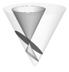
Figure 2: The 3-web in shape space for the triatomic molecule.

Proposition 2.3.

Consider a triatomic molecule in a stable non-degenerate equilibrium configuration $Q_{0}$. For any $\epsilon>0$ sufficiently small, there exist at least 3 distinct normal relative equilibria at $\pi(Q_{j})$ with $|\pi(Q_{0})-\pi(Q_{j})|<\epsilon$ for $j=1,2,3$.

Remark 2.2.

More generally suppose that $x_{0}$ is a stable non-degenerate equilibrium in shape space. For a given coadjoint orbit suppose the $k$-web is regular at $x_{0}$. Then in a sufficiently small neighbourhood of $x_{0}$ the equilibrium bifurcates into a family of at least $k$ normal RE.

2.3 The Full-Body Satellite Problem

Consider the motion of a rigid body in $\mathbf{R}^{3}$ subject to a central force directed through the origin. The configuration space may be taken to be $\mathbf{SE}(3)=\mathbf{SO}(3)\ltimes\mathbf{R}^{3}$, whereby a configuration of the body is identified with the Euclidean motion $(a,d)$ which sends the fixed frame $\mathcal{F}$ in space to the body frame $a\mathcal{F}+d$.

Consider the action of $\mathbf{SO}(3)$ on the left given by $g(a,d)=(ga,gd)$. An orbit-map for this action is

$$\pi\colon\mathbf{SE}(3)\longrightarrow\mathbf{R}^{3};\quad(a,d)\longmapsto x=-a^{-1}d.$$

The vector $x$ is the origin of the space-frame viewed from within the body frame. We choose $\sigma\colon x\mapsto(\text{Id},-x)$ to be a section for this principal bundle and consider the kinetic energy generated by $\omega\in\mathfrak{so}(3)$ acting on the configuration $\sigma(x)$

$$\frac{1}{2}\int|\omega z-\omega x|^{2}dz=\frac{1}{2}\int\left(|\omega z|^{2}-2\langle\omega z,\omega x\rangle+|\omega x|^{2}\right)dz.$$

The integral is taken over the points $z$ belonging to the body in the body frame. If we suppose that the origin of the body frame coincides with the centre of mass of the body, then $\int zdz=0$ and the kinetic energy simplifies to

$$\frac{1}{2}\langle\mathbb{I}_{0}(\omega),\omega\rangle+\frac{1}{2}|\omega x|^{2}$$

where $\mathbb{I}_{0}$ is the constant inertia tensor for the body in the body frame, and where we are supposing for simplicity that the body has unit mass. By once again identifying $\omega$ with an element in $\mathbf{R}^{3}$ we can write the kinetic energy as $\frac{1}{2}\langle\omega,\mathbb{I}_{x}(\omega)\rangle$ where the symmetric matrix

$$\mathbb{I}_{x}=\mathbb{I}_{0}+|x|^{2}\text{Id}-xx^{T}$$ (2.4)

is the inertia tensor. We may suppose that the body frame is chosen so that $\mathbb{I}_{0}$ is diagonal, with distinct entries $I_{1}<I_{2}<I_{3}$, the principal moments of inertia of the body.

Proposition 2.4.

The 3-web on shape space is given by the surfaces

$$1=\sum_{j=1,2,3}\frac{x_{j}^{2}}{(I_{k}-\lambda)+|x|^{2}}$$ (2.5)

for $\lambda\geq I_{1}$ a given eigenvalue of $\mathbb{I}_{x}$. The subset of shape space in which the inertia tensor admits repeated eigenvalues are the curves

$$x_{k}^{2}(I_{l}-I_{m})+x_{l}^{2}(I_{k}-I_{m})=(I_{l}-I_{m})(I_{l}-I_{m}),\quad x_{m}=0,$$ (2.6)

for $k,l,m=1,2,3$ all distinct.

Proof.

One may verify that the characteristic polynomial of $\mathbb{I}_{x}$ is the numerator obtained from Eq. (2.5) after multiplying up by the denominators.

Suppose $\mathbb{I}_{x}$ has a repeated eigenvalue $\lambda$. The eigenspace must contain an eigenvector $\omega$ orthogonal to $x$, and so $\mathbb{I}_{x}(\omega)=\mathbb{I}_{0}\omega+|x|^{2}\omega=\lambda\omega$, which implies that $\omega$ is along a principal direction, let’s say $e_{m}$, and that $\lambda=I_{m}+|x|^{2}$. Now take a second independent eigenvector $\nu$, which we may suppose is orthogonal to $\omega$. Then

$$\mathbb{I}_{x}(\nu)=\mathbb{I}_{0}\nu+|x|^{2}\nu-x\langle x,\nu\rangle=\lambda\nu=(I_{m}+|x|^{2})\nu,$$ (2.7)

which implies $\mathbb{I}_{0}\nu-I_{m}\nu=x\langle x,\nu\rangle$. It follows that $\nu$ is proportional to $D^{-1}x$, where $D=\text{diag}(I_{k}-I_{m},I_{l}-I_{m})$ with respect to the basis $\{e_{k},e_{l}\}$. Substituting this $\nu$ back into Eq. (2.7) yields Eq. (2.6). ∎

The surfaces defined in Eq. (2.5) are quartic in $x$ and come in three families depending on which of the intervals $(I_{1},I_{2})$, $(I_{2},I_{3})$, or $(I_{3},\infty)$ the eigenvalue $\lambda$ belongs to (and three singular leaves for when $\lambda=I_{1},I_{2},I_{3})$. The regular leaves are displayed in Figure 3.

• The leaves are empty for $\lambda<I_{1}$. Indeed, the inertia in space can never be less than the smallest moment of inertia of the body itself. For $\lambda=I_{1}$ the leaf is the point at the origin.

• For $I_{1}<\lambda<I_{2}$ the leaf is a topological cylinder aligned with the $x_{1}$-axis.

• For $I_{2}<\lambda<I_{3}$ the leaf consists of two sheets joined together with a topological sphere at 4 singular points in the plane $x_{1}=0$.

• For $\lambda>I_{3}$ the leaf is two concentric topological spheres joined together at 4 nodal singularities in the plane $x_{2}=0$. Figure 3 shows two cutaways of this surface to highlight this property.

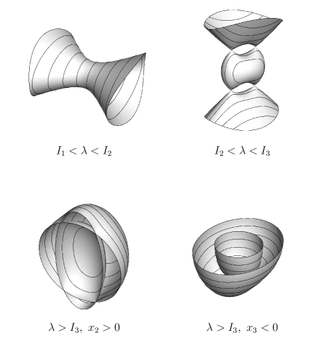
Figure 3: The 3-web in shape space for the full-body satellite problem.

Remark 2.3.

The curves in Eq. (2.6) are empty if $I_{m}$ is the largest moment of inertia. Therefore, there are 3 curves of repeated eigenvalues: an ellipse in the plane $x_{1}=0$, and two hyperbolae in the plane $x_{2}=0$. Notice how these curves match the singular points of the web. Indeed, singular points of a web are indicative of repeated eigenvalues.

2.3.1 Great-Circle Relative Equilibria

A great-circle RE is a RE for which the centre of mass of the body remains in the plane of rotation [23]. Equivalently, $\omega$ is orthogonal to $x$. From Eq. 2.4 this implies that $\omega$ is parallel with a principal direction. In fact, we have

Lemma 2.1.

A relative equilibria at $x\in\mathbf{R}^{3}$ is a great-circle motion if and only if $x$ belongs to a principal plane, say orthogonal to $e_{m}$, and the corresponding angular velocity $\omega$ is parallel to $e_{m}$ with inertia $\lambda=I_{m}+|x|^{2}$.

Consider the orbit of a body sufficiently far away from the origin so that its orbital inertia is larger than any moment-of-inertia of the body itself. From topological considerations of the leaf alone we are able to deduce the following result of [24].

Proposition 2.5.

For any sufficiently large $\lambda>I_{3}$ there exist at least two normal relative equilibria for a rigid body in an attractive central-force with potential $V$. If the body has a plane of symmetry, then it has at least 2 great-circle relative equilibria. If the body is symmetric with respect to 2 planes of symmetry, then it has at least 4 great-circle relative equilibria, and if the body has 3 planes of symmetry then it has at least 12 great-circle relative equilibria (all solutions defined up to time-reversal).

Proof.

We suppose the body does not intersect the origin in space. Therefore, both V and $\lambda$ increase in the radial direction, and hence, if $\nabla V$ and $\nabla\lambda$ are parallel, then they must be in the same direction. It follows that all critical points of the potential and inertia are normal RE.

On the leaf $\lambda>I_{3}$ there must exist a minimum of $V$ on the inner sphere, and a maximum on the outer sphere (neither of which can coincide with the 4 singular conical points of the leaf).

The intersection of the leaf with the principal plane orthogonal to $e_{m}$ is the union of an ellipse and the circle $|x|^{2}=\lambda-I_{m}$. The potential must have at least two critical points on such a circle, and hence, from symmetry considerations and Lemma 2.1 the result follows. ∎

Remark 2.4.

The surfaces $\lambda<I_{3}$ are applicable to extremely large satellites, such as an orbital ring or hollow shell, whose extent encompasses the origin in space. The topology of the leaves suggest that, generically, there are at least 2 RE for $\lambda_{1}<\lambda<I_{2}$, and at least 4 RE for $I_{2}<\lambda<I_{3}$. There is also the prospect of abnormal RE: do there exist bodies with distinct moments-of-inertia which admit abnormal RE?

3 The Spherical 3-Body Problem

Consider 3 particles $q_{1},q_{2},q_{3}$ on the unit sphere and let $Q$ be the matrix whose $j$^th-column is $q_{j}$. An orbit map for the action of $\textbf{O}(3)$ on $\textbf{S}^{2}\times\textbf{S}^{2}\times\textbf{S}^{2}$ is given by sending $(q_{1},q_{2},q_{3})$ to

$$\pi(Q)=3\text{Id}-Q^{T}Q=\begin{pmatrix}2&-x_{1}&-x_{2}\\ -x_{1}&2&-x_{3}\\ -x_{2}&-x_{3}&2\end{pmatrix}$$ (3.1)

where

$$x_{1}=\cos\theta_{12},\quad x_{2}=\cos\theta_{13},\quad x_{3}=\cos\theta_{23},$$

and $\theta_{ij}$ is the angle subtended between $q_{i}$ and $q_{j}$. The $x_{j}$ are bounded between $-1$ and $1$ and satisfy the the inequality

$$\det Q^{T}Q=|\langle q_{1},q_{2}\times q_{3}\rangle|^{2}\geq 0.$$

The shape space is therefore the (curvy) tetrahedron $\mathcal{T}\subset\mathbf{R}^{3}$ given by the cubic inequality

$$1+2x_{1}x_{2}x_{3}-x_{1}^{2}-x_{2}^{2}-x_{3}^{2}\geq 0.$$ (3.2)

It is helpful to see which parts of the tetrahedron correspond to given configurations of the particles.

• The vertices of $\mathcal{T}$ are the colinear configurations (which we should technically exclude since here the action is not free). The top vertex $P$ at $x_{1}=x_{2}=x_{3}=1$ is the triple collision, and the other vertices are pairs of binary collisions with the third particle antipodal to the pair.

• The three edges from $P$ correspond to binary collisions, and the other three edges to antipodal pairs.

• The boundary $\partial\mathcal{T}$ consists of the coplanar configurations. The faces with common vertex $P$ are those configurations where the particles lie in a common half-plane. Those which do not lie in a common half-plane correspond to the bottom face $F$ opposite $P$.

• The interior of the tetrahedron are those configurations where the particles are in general position.

Permuting the particles generates the $\mathbf{S}_{3}$-action which permutes the coordinates $x_{1},x_{2},x_{3}$ and fixes $P$. In addition, the $\mathbf{Z}_{2}$-symmetry which negates a particle’s position negates a pair of $x_{j}$-coordinates and transposes $P$ with another vertex. Taken together these generate the order-24 group $\mathbf{T_{d}}$ of tetrahedral symmetries.

Remark 3.1.

We shall actually be considering the quotient by $\mathbf{SO}(3)$. There is an additional invariant $\Delta=\langle q_{1},q_{2}\times q_{3}\rangle$ which satisfies $\Delta^{2}=\det Q^{T}Q$. The shape space is therefore two copies $\mathcal{T}_{\pm}$ corresponding to the sign of $\Delta$, and the union is taken over their boundary for $\Delta=0$. Topologically the shape space is a 3-sphere. However, since the $\mathbf{Z}_{2}$-symmetry which negates $(q_{1},q_{2},q_{3})$ interchanges $\mathcal{T}_{+}$ with $\mathcal{T}_{-}$, it will suffice to deal with a single copy of $\mathcal{T}$.

3.1 A Web of Cayley Cubics on the 3-Sphere

We shall now suppose that the three particles each have unit mass. In the same way that we derived Eq. (2.1) the inertia tensor is

$$\mathbb{I}_{Q}=3\text{Id}-QQ^{T}.$$ (3.3)

Proposition 3.1.

The 3-web on $\mathcal{T}$ is the family of Cayley cubics

$$(\lambda-2)^{3}+2x_{1}x_{2}x_{3}-(\lambda-2)(x_{1}^{2}+x_{2}^{2}+x_{3}^{2})=0$$ (3.4)

for $\lambda\in[0,3]$ a given eigenvalue of $\mathbb{I}_{Q}$. The inertia tensor has twice-repeated eigenvalues along the four lines which originate at a vertex and go through the midpoint of the opposite face. There is a triple-repeated eigenvalue at the centre $x_{1}=x_{2}=x_{3}=0$ of the tetrahedron where these lines intersect.

Proof.

The characteristic polynomials of $\pi(Q)$ and $\mathbb{I}_{Q}$ coincide, and thus, the subset of $\mathcal{T}$ for a constant eigenvalue $\lambda$ are the surfaces $\chi(\lambda)=0$, where $\chi(\lambda)$ is the characteristic polynomial of $\pi(Q)$ and is given by the left hand side of Eq. (3.4).

A repeated eigenvalue occurs whenever the discriminant

$$(x_{1}^{2}+x_{2}^{2}+x_{3}^{2})^{3}-27x_{1}^{2}x_{2}^{2}x_{3}^{3}$$

of $\chi$ is zero. By the AM-GM inequality this only holds when $x_{1}^{2}=x_{2}^{2}=x_{3}^{2}$. ∎

The surface defined by taking the equality in Eq. (3.2) is Cayley’s Nodal Cubic Surface. It consists of a curvy tetrahedron $\partial\mathcal{T}$ with nodal singularities at the vertices, around which 4 conical regions emanate outwards. For $\lambda\neq 2$ the surface defined by Eq. (3.4) is a dilation of the Cayley cubic by a factor of $\lambda-2$. Notice that for $\lambda<2$ this scaling is negative and inverts the surface, producing a tetrahedron dual to $\mathcal{T}$. The intersections of these surfaces with $\mathcal{T}$ produce the leaves of the 3-web and are shown in Figure 4.

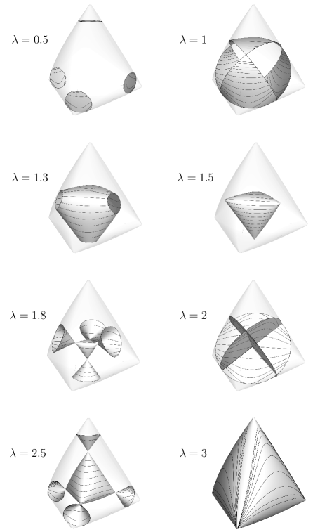
Figure 4: The 3-web of Cayley cubics for the spherical 3-body problem. The contours are for the cotangent potential.

• For $\lambda=0$ the leaf is singular and consists of the four vertices of $\mathcal{T}$. For $0<\lambda<1$ the leaf becomes 4 disconnected disk-like regions near each vertex.

• At $\lambda=1$ the 4 disks connect to each other pairwise at the midpoints of the edges of $\mathcal{T}$. For $1\leq\lambda\leq 3/2$ the leaf is a connected surface.

• For $\lambda=3/2$ the leaf is a curvy tetrahedron dual to $\mathcal{T}$ and contained entirely inside $\mathcal{T}$, with its vertices at the midpoints of the faces of $\partial\mathcal{T}$. As $\lambda$ grows the dual tetrahedron shrinks inside $\mathcal{T}$ and its 4 conical regions grow.

• The leaf degenerates at $\lambda=2$ into union of planes $x_{1},x_{2},x_{3}=0$. For $2<\lambda\leq 3$ the leaf is a dilation of $\partial\mathcal{T}$ and continues to grow until $\lambda=3$, at which point the leaf coincides with the boundary of $\mathcal{T}$. For $\lambda>3$ the intersection is empty and the leaves are no longer defined.

3.2 Classification of Relative Equilibria for Equal Masses

Theorem 3.

Consider 3 particles of equal mass constrained to a sphere and mutually interacting via a strictly attractive potential-force depending only on the angle between particles. The system admits the following types of relative equilibrium solutions.

1. Coplanar: (i) with one particle on the axis of rotation and the other two particles each located an angle $\theta\in(0,\frac{\pi}{2})\cup(\frac{\pi}{2},\frac{2\pi}{3})$ either side of the axis; (ii) with one particle orthogonal to the axis of rotation and the other two particles located at an angle $\theta\in(\frac{2\pi}{3},\pi)$ either side of the first particle; (iii) an equilibrium solution with the particles at the vertices of an equilateral triangle, and a family of relative equilibria obtained by spinning this configuration in the plane.

2. General Position: (i) with the particles at the vertices of a spherical equilateral triangle with internal angles $\phi\in(0,\frac{2\pi}{3})$, rotating about the axis through the midpoint of the triangle.

These relative equilibria are normal expect for abnormal solutions of Type 1(i) for $\theta=\frac{\pi}{3}$, and Type 2(i) for $\phi=\frac{\pi}{2}$. For the specific choice of cotangent potential

$$V=-\cot\theta_{12}-\cot\theta_{13}-\cot\theta_{23}$$

the relative equilibria are completely classified by two additional subtypes of normal relative equilibria.

1. (iv) Scalene: with the particles belonging to a half plane containing the axis of rotation, where the angles $\alpha$ and $\beta$ from the middle particle to the other two satisfy

   $$\sin 2\beta(\csc^{2}\alpha+\csc^{2}\gamma)+\sin 2\gamma(\csc^{2}\alpha-\csc^{2}\beta)=\sin 2\alpha(\csc^{2}\beta+\csc^{2}\gamma),$$ (3.5)

   for $\gamma=\alpha+\beta$ and $\alpha\neq\beta$.

2. (ii) Isosceles: with two particles separated by an angle $\beta$ and the third particle located at an angle $\alpha\neq\beta$ from each of the two particles, where $\alpha,\beta\in(-\pi,\pi)$ satisfy

   $$\cos\alpha(2\sin^{6}\alpha-\sin^{6}\beta)=\sin^{3}\alpha\sin^{3}\beta\cos\beta.$$ (3.6)

Figure 5: Coplanar relative equilibria.

We shall prove this theorem by classifying the critical points $\operatorname{Crit}(V,\lambda)$. Of course, points in $\operatorname{Crit}(V,\lambda)$ are not necessarily abnormal RE, as one must check that the gradients of $V$ and $\lambda$ have the same direction. We leave this routine task as an exercise to the interested reader.

3.2.1 Coplanar Configurations

The reduced potential is invariant under the $\mathbf{Z}_{2}$-symmetry which interchanges $\mathcal{T}_{+}$ with $\mathcal{T}_{-}$. Therefore, the points of $\operatorname{Crit}({V},\lambda)$ belonging to $\partial\mathcal{T}$ are equivalently the points of $\operatorname{Crit}({V}|_{\partial\mathcal{T}},\lambda|_{\partial\mathcal{T}})$. It is also invariant under the $\mathbf{S}_{3}$-symmetry fixing $P$, including the reflections which transpose two vertices of $F$. The set of critical points therefore contains the intersections of $\partial\mathcal{T}$ with the planes of symmetry $x_{i}=x_{j}$ for any choice of potential.

Proof of Theorem 3 for normal RE of Type 1.

Observe from Eq. (3.4) that the intersection of any leaf from the web with $\partial\mathcal{T}$ is the same as the intersection of $\partial\mathcal{T}$ with a sphere centred at the origin. Therefore, for the cotangent potential we must classify the critical points of

$$V=-\cot\theta_{12}-\cot\theta_{13}-\cot\theta_{23},\quad\text{and}\quad r=\cos^{2}\theta_{12}+\cos^{2}\theta_{13}+\cos^{2}\theta_{23}$$

restricted to $\partial\mathcal{T}$. For configurations in $F$ we have $\theta_{23}=2\pi-\theta_{12}-\theta_{13}$. This allows us to write $V$ and $r$ in terms of $(\theta_{12},\theta_{13})$. The equation $\nabla V\times\nabla r=0$ boils down to

$$\sin(\theta_{12}-\theta_{13})\sin(\theta_{12}-\theta_{23})\sin(\theta_{13}-\theta_{23})=0$$ (3.7)

which gives the coplanar configurations of Type 1(ii). For coplanar configurations not in $F$ we now have $\theta_{23}=\theta_{12}+\theta_{13}$ (assuming that the second particle is in the middle of the half-plane containing all three). Writing $\nabla V\times\nabla r=0$ in terms of $(\alpha,\beta)=(\theta_{12},\theta_{13})$ yields Eq. (3.5) whose solutions are shown in Figure 6. The curve $\alpha=\beta$ gives the RE of Type 1(i), and the other curve gives the scalene family of Type 1(iv)

Figure 6: Curve of scalene-coplanar configurations.

∎

Remark 3.2.

The boundary $\partial\mathcal{T}$ is itself the leaf $\lambda=3$, and is the fixed-point set of the $\mathbf{Z}_{2}$-symmetry which interchanges $\mathcal{T}_{+}$ with $\mathcal{T}_{-}$. It follows that $\nabla\lambda=0$ for this eigenvalue on the boundary. For this reason, the equilibrium point at the midpoint of $F$ (a local minimum of the potential) is also a normal RE for any $L$ an eigenvector with eigenvalue $\lambda=3$. These are the RE of Type 1(iii).

3.2.2 Abnormal Relative Equilibria

To find abnormal RE we must solve Eq. (1.7) for when $L$ ranges over the eigenspace for a repeated eigenvalue.

Proposition 3.2.

Along the 4 lines in $\mathcal{T}$ where $\mathbb{I}_{x}$ has a repeated eigenvalue, the map

$$L\longmapsto\nabla\big{\langle}L,\mathbb{I}_{x}^{-1}L\rangle$$

from the repeated eigenspace into $T_{x}\mathcal{T}$ is a 2-1 map with image

$$\begin{cases}T_{x}\mathcal{T},&\text{for $x$ at the centre of $\mathcal{T}$}\\[4.30554pt] T_{x}\partial\mathcal{T},&\text{for $x$ at the midpoint of $F$}\\[4.30554pt] \mathcal{C},&\parbox[t]{199.16928pt}{for $x$ elsewhere on the line through $P$.}\end{cases}$$

Here $\mathcal{C}$ is the cone of vectors $X_{1}(\partial/\partial x_{1})+X_{2}(\partial/\partial x_{2})+X_{3}(\partial/\partial x_{3})$ satisfying

$$X_{1}X_{2}+X_{1}X_{3}+X_{2}X_{3}=0,\quad\text{for}\quad X_{1}+X_{2}+X_{3}\geq 0.$$ (3.8)

Along any of the other lines we may apply the $\mathbf{Z}_{2}$-symmetry exchanging $P$ with another vertex by negating a pair of $(x_{1},x_{2},x_{3})$.

Proof.

By differentiating the identity $\mathbb{I}_{x}\circ\mathbb{I}_{x}^{-1}=\text{Id}$ at $x_{0}$ we have

$$\nabla\langle L,\mathbb{I}_{x}^{-1}L\rangle=-\nabla\langle L,\mathbb{I}_{x_{0}}^{-1}\circ\mathbb{I}_{x}\circ\mathbb{I}_{x_{0}}^{-1}(L)\rangle=-\lambda^{-2}\nabla\langle L,\mathbb{I}_{x}L\rangle.$$ (3.9)

For $x$ in the interior of $\mathcal{T}$ the matrix $Q$ is non-singular, and so $x=\pi(Q)\mapsto\sqrt{Q^{T}Q}$ is a differentiable local section $\sigma$. For this choice of section $\mathbb{I}_{Q}=\pi(Q)$, and so from Eq. (3.9) it suffices to compute

$$-\nabla\langle L,\pi(Q)L\rangle$$

for $L$ an eigenvector of $\pi(Q)$ with a repeated eigenvalue.

The situation on the boundary is a little different since $(x_{1},x_{2},x_{3})$ fails to be a coordinate chart on shape space. Instead, we take a chart $(\theta_{12},\theta_{13},\varphi)$ with a specific section $q_{1}=(1,0,0)^{T}$, $q_{2}=(\cos\theta_{12},\sin\theta_{12},0)^{T}$, and $q_{3}=(\cos\varphi\cos\theta_{13},\cos\varphi\sin\theta_{13},\sin\varphi)^{T}$ and compute (3.9) directly.

∎

Proof of Theorem 3 for abnormal RE.

It follows from the proposition that exactly one abnormal RE exists (up to time-reversal) at the centre of $\mathcal{T}$ and at the midpoints of the faces.

The gradient of the reduced potential is proportional to $(1,1,1)$ when evaluated along any of the four lines in the interior of $\mathcal{T}$. Hence, for $x$ elsewhere along these lines there are no abnormal RE since $\nabla{V}$ does not belong to the cone $\mathcal{C}$.

∎

3.2.3 General Position Configurations

Lemma 3.1.

For the cotangent potential every point of $\operatorname{Crit}({V},\lambda)$ in the interior of $\mathcal{T}$ is isosceles. That is to say, $x_{i}=x_{j}$ for a pair of coordinates.

Proof.

Consider a leaf of the web. We immediately discount the degenerate leaf $\lambda=2$ since ${V}$ restricted to the coordinate planes $x_{k}=0$ is regular everywhere.

For $\lambda\neq 2$ the component of the web which is a curvy tetrahedron admits a parametrisation

$$x_{j}=(\lambda-2)\cos\phi_{j},\quad\text{for}\quad\phi_{1}+\phi_{2}+\phi_{3}=0.$$ (3.10)

Finding critical points of ${V}$ restricted to the leaf therefore becomes the Lagrange multiplier problem

$$(\lambda-2)\sin\phi_{j}=\kappa\left[1-(\lambda-2)^{2}\cos^{2}\phi_{j}\right]^{3/2}.$$

Squaring both sides and rearranging yields

$$\frac{(\lambda-2)^{2}-x_{j}^{2}}{\kappa^{2}}=(1-x_{j}^{2})^{3}.$$

Note that this is a cubic in $x_{j}^{2}$. Suppose that the solutions $x_{1},x_{2},x_{3}$ are distinct. Then $x_{1}^{2},x_{2}^{2},x_{3}^{2}$ must be the three solutions to the cubic, and so their sum must be the coefficient of $x_{j}^{4}$, which is simply $3$. The only $x$ in $\mathcal{T}$ for which $x_{1}^{2}+x_{2}^{2}+x_{3}^{2}=3$ are the vertices.

For the conical components of the web we repeat the argument but using the parametrisation $x_{j}=\pm(\lambda-2)\cosh\phi_{j}$. ∎

Proof of Theorem 3 for RE of Type 2.

The line through $P$ and the midpoint of $F$ is fixed by the $\mathbf{S}_{3}$-symmetry. Therefore, for any choice of potential this line belongs to $\operatorname{Crit}({V},\lambda)$, and for a strictly attractive potential corresponds to a family of normal RE of Type 2(i).

To classify the remaining points of $\operatorname{Crit}({V},\lambda)$ in the interior of $\mathcal{T}$ it suffices from the previous lemma to consider the plane $x_{1}=x_{3}$. In this plane Eq. (3.4) factors as

$$\left((\lambda-2)+x_{2}\right)\left((\lambda-2)^{2}-(\lambda-2)x_{2}-2x_{1}^{2}\right)$$ (3.11)

and the cotangent potential becomes ${V}=-2x_{1}(1-x_{1}^{2})^{-1/2}-x_{2}(1-x_{2}^{2})^{-1/2}$. There are no critical points along the line $x_{2}=2-\lambda$, however along the parabolae defined by the quadratic factor in Eq. (3.11) we find that the critical points are those which satisfy

$$\pm(1-x_{2}^{2})^{3/2}\sqrt{8x_{1}^{2}+x_{2}^{2}}=4x_{1}(1-x_{1}^{2})^{3/2}-x_{2}(1-x_{2}^{2})^{3/2}.$$ (3.12)

This defines three curves in the plane shown in Figure 7, including the line $x_{1}=x_{2}=x_{3}$ of equilateral solutions of Type 2(i), and the curves of Type 2(ii). By squaring both sides of this equation and writing $x_{1}=\cos\alpha$ and $x_{2}=\cos\beta$ we obtain Eq.(3.6). ∎

Figure 7: The intersection of $\mathcal{T}$ with the plane $x_{1}=x_{3}$. Shown are the curves of Type 2 relative equilibria.

Remark 3.3.

It would be interesting to repeat the classification for other choices of potential. See the discussion in [2] regarding the different laws of gravitation which can be chosen in curved space. Another application could be to the Thomson Problem of point charges on the sphere. Problem 7 in Smale’s list [22] concerns the equilibria, however the relative equilibria have not garnered as much attention. What are the RE for 3 equal-mass particles with charges $(e_{1},e_{2},e_{3})$ interacting via the Coulomb potential?

Finally, we remark that one can generalise our web formalism to the case of non-equal masses. The 3-web is still a family of Cayley cubics, albeit with more variation in $\lambda$. Furthermore, they lose their tetrahedral symmetry, and the subset of repeated eigenvalues for the inertia tensor is a more complicated set of curves. In principle, one can still use Theorem 1 to show the existence of certain families of RE, however, attempts at a full classification quickly devolve into an ominous heap of algebra.

4 Larger Symmetry Groups

For more general symmetry groups there are more solutions to Eq. 1.11 than just the eigenvectors of $\mathbb{I}_{x}$. For a fixed $x$ this equation is quadratic in $L\in\mathfrak{g}^{*}$ and its solutions depend very delicately upon the nature of the Lie algebra $\mathfrak{g}$ and the inertia tensor. Furthermore, for larger groups there is a greater variety of coadjoint orbits. Consequently, there exists a family of webs parametrised by the equivalence classes of coadjoint orbits in $\mathfrak{g}^{*}$ modulo scaling.

4.1 The Case of the Riemann Ellipsoids

Consider a spherical droplet of incompressible fluid at time $t=0$. In the linear approximation the configuration of the droplet at time $t$ is determined by a $Q(t)\in\mathbf{SL}(3)$, whereby the fluid particle initially at $x_{0}$ is now at $Q(t)x_{0}$. If the fluid is homogeneous and has unit mass, then the kinetic energy is $\operatorname{Tr}(\dot{Q}^{T}\dot{Q})$, which we observe to be invariant under both left and right multiplication by $\mathbf{O}(3)$.

The singular values $\{x_{1},x_{2},x_{3}\}$ of $Q$ are invariant under this action, and so we may identify shape space with $\mathcal{B}=\{x_{1},x_{2},x_{3}\geq 0~{}|~{}x_{1}x_{2}x_{3}=1\}$. Strictly speaking, shape space is actually the quotient of this set by permutations, however we won’t come to any harm if we proceed by working locally in a region where the singular values are distinct, as in Remark 2.1.

We take a section over shape space by sending the singular values to the matrix $\text{diag}(x_{1},x_{2},x_{3})$. If we identify elements of $\mathfrak{so}(3)$ with vectors in $\mathbf{R}^{3}$ then for this choice of section the inertia tensor is the block matrix

$$\mathbb{I}_{x}=\begin{pmatrix}A&B\\ B&A\end{pmatrix},~{}\text{for}~{}A=\text{diag}(a_{1},a_{2},a_{3}),~{}\text{and}~{}B=\text{diag}(b_{1},b_{2},b_{3}),$$ (4.1)

where $a_{k}=x_{l}^{2}+x_{m}^{2}$ and $b_{k}=-2x_{l}x_{m}$ for distinct $k,l,m$.

The vectors $\omega,\xi\in\mathfrak{so}(3)$ are the angular velocity and vorticity of the fluid. Write the image of $(\omega,\xi)$ under $\mathbb{I}_{x}$ as $(L,\Omega)$. The terminology in the following lemma is borrowed from [7].

Lemma 4.1.

For distinct $x_{1},x_{2},x_{3},$ the solutions to $[(\omega,\xi),(L,\Omega)]=0$ come in two types:

1. The vectors $\omega$ and $\xi$ are each parallel to a principal direction $e_{k}$ and have arbitrary length. These solutions are said to of Type $\textbf{S}_{(k)}$.

2. For any $\omega$ not parallel with $e_{l}$ or $e_{m}$ but belonging to the plane spanned by $e_{l}$ and $e_{m}$, there exist exactly two solutions for $\xi$, unless

   $$2x_{k}=\pm x_{l}\pm x_{m},$$

   in which case there exists precisely one. These solutions are said to be of Type R.

Proof.

The Lie bracket $[(\omega,\xi),(L,\Omega)]$ is $(\omega\times L,\xi\times\Omega)$, and so for this to be zero we require

$$\begin{cases}A\omega+B\xi&=s\omega\\ B\omega+A\xi&=t\xi\end{cases}$$ (4.2)

for some $s,t\in\mathbf{R}$. We can solve for $\xi$ in the first equation and then substitute this into the second to find that $C\omega=0$, where $C=B^{2}-A^{2}+(s+t)A-(st)\text{Id}$. This matrix is diagonal, and so its kernel is either: a principle direction, giving solutions of Type S; or, a principal plane. In the latter, for $e_{l}$ and $e_{m}$ to both belong to the kernel of $C$ we require $(s,t)=(\mu_{\pm},\mu_{\mp})$, where

$$\mu_{\pm}=\frac{1}{2}\left(-2x_{k}^{2}+x_{l}^{2}+x_{m}^{2}\pm\sqrt{D}\right),$$ (4.3)

and $D$ is the product of $2x_{k}\mp x_{l}\mp x_{m}$ over the 4 choices of signs (which we note to be non-negative). ∎

Proposition 4.1.

For the coadjoint orbit $\mathcal{O}=\mathbf{S}^{2}_{\rho_{1}}\times\mathbf{S}^{2}_{\rho_{2}}$ the web $\mathcal{W}_{\mathcal{O}}$ on $\mathcal{B}$ consists of:

1. The level sets of

   $$\Lambda(x)=\frac{(\rho_{1}^{2}+\rho_{2}^{2})(x_{k}^{2}+x_{l}^{2})\pm 4\rho_{1}\rho_{2}x_{k}x_{l}}{(x_{k}^{2}-x_{l}^{2})^{2}}$$ (4.4)

   defined on $x_{k}\neq\pm x_{l}$, and for each choice of coordinate pair $(k,l)$ and $\pm$-sign.

2. The level sets of

   $$\Lambda(x)=\frac{\rho_{1}^{2}}{\mu_{\pm}}+\frac{\rho_{2}^{2}}{\mu_{\mp}}$$ (4.5)

   defined in a particular region, and for each choice of principal plane and $\pm$-sign.

Proof.

Recall that the level sets of the web are given by

$$\Lambda(x)=\langle L,\omega\rangle+\langle\Omega,\xi\rangle$$ (4.6)

for $L=s\omega$ and $\Omega=t\xi$ as in Lemma 4.1. For solutions of Type $\text{S}_{k}$ the angular velocities $\omega=\omega^{k}e_{k}$ and $\xi=\xi^{k}e_{k}$ satisfy the system in Eqs. (4.2), which becomes

$$\begin{cases}a_{k}\omega^{k}+b_{k}\xi^{k}&=\pm\rho_{1},\\ b_{k}\omega^{k}+a_{k}\xi^{k}&=\pm\rho_{2}.\end{cases}$$

We can solve this directly and obtain Eq. 4.4 by substituting the solutions into Eq. (4.6).

For solutions of the second type, we observe that for any $\omega$ belonging to a principal plane, there exist unique solutions to Eqs. (4.2) for $(s,t)=(\mu_{+},\mu_{-})$. However, for $L=s\omega$ with absolute value $\rho_{1}$, there is no guarantee that $\Omega=t\xi=tB^{-1}(s\omega-A\omega)$ should have absolute value $\rho_{2}$. Therefore, there is only a solution belonging to $\mathcal{O}$ whenever $x$ belongs to the region of shape space for which

$$\frac{\rho_{1}}{\rho_{2}}~{}\text{is between}~{}\left|\frac{\mu_{+}}{\mu_{-}}\right|\left|\frac{b_{m}}{\mu_{+}-a_{m}}\right|~{}\text{and}~{}\left|\frac{\mu_{+}}{\mu_{-}}\right|\left|\frac{b_{l}}{\mu_{+}-a_{l}}\right|.$$ (4.7)

∎

An example of a 6-web defined in Eq. (4.4) is shown in Figure 8 (where we have identified $\mathcal{B}$ with the plane $z_{1}+z_{2}+z_{3}=0$ by taking $z_{k}=\log x_{k}$). Apparent in this figure is the $\mathbf{S}_{3}$-symmetry which arises from permuting the singular values of $Q$.

Remark 4.1.

Dedekind famously observed [5] that if $Q(t)$ was a RE then so was the transpose $Q^{T}(t)$. Taking the transpose of a RE swaps the angular velocity and vorticity vectors, and therefore swaps $L\leftrightarrow\Omega$. We can see this symmetry at the level of webs by observing that the $\mathcal{W}_{\mathcal{O}}$ in Proposition 4.1 is invariant with respect to $\rho_{1}\leftrightarrow\rho_{2}$.

The RE for a gravitating ellipsoid were classified by Riemann [18]. Although it is not our intention to reproduce such a classification—it is a significant undertaking [3, 4]—we will classify those of Type S, since the proof using webs is so short that it would be a shame not to include. The only fact we shall need to know about the potential $V$ is that its gradient at $x$ is a positive scalar multiple of $x$ (see [7, p. 263]).

Figure 8: The 6-web for RE of Type S with $\rho_{1}=\rho_{2}$.

Proposition 4.2.

For a gravitating ellipsoid with $x_{1}>x_{2}>x_{3}$ there exists exactly one relative equilibrium of Type $S_{3}$ (up to time-reversal and transpose symmetry). If $x_{2}<1$ then there exists an additional relative equilibrium of Type $S_{2}$.

Proof.

Let $k,l,m=1,2,3$ be distinct and write $\Lambda(x)$ in Eq. (4.4) as

$$(\rho_{1}^{2}+\rho_{2}^{2})f(x)\pm 2\rho_{1}\rho_{2}g(x).$$

It follows that $\nabla\Lambda$ is a positive scalar multiple of $\nabla f+p\nabla g$ for $p\in(-1,1)$. For $x_{k}>x_{l}$ one can show that

$$\hat{u}=\frac{1}{\sqrt{2}}\left(-\frac{\partial}{\partial x_{k}}+\frac{\partial}{\partial x_{l}}\right),\quad\text{and}\quad\hat{v}=\frac{1}{\sqrt{2}}\left(-\frac{\partial}{\partial x_{k}}-\frac{\partial}{\partial x_{l}}\right)$$

are the normalisations of $\nabla f+\nabla g$ and $\nabla f-\nabla g$, respectively. Therefore, a normal RE of Type $S_{m}$ exists if and only if there exist $\alpha,\beta>0$ for which $-\nabla{V}=\alpha\hat{u}+\beta\hat{v}$. Since $\nabla{V}$ is a positive scalar multiple of $x$, the result follows by considering the solutions for $\alpha$ and $\beta$ in the system

$$\begin{cases}-x_{k}&=-\alpha-\beta+\kappa x_{l}x_{m},\\ -x_{l}&=\alpha-\beta+\kappa x_{k}x_{m},\\ -x_{m}&=\kappa x_{k}x_{l},\end{cases}$$ (4.8)

where $\kappa$ is a Lagrange multiplier for the surface $x_{1}x_{2}x_{3}=1$.

∎

4.2 Higher dimensional N-body systems

Consider $n$ particles in general position in Euclidean space $\mathbf{R}^{d}$. The configuration is determined by the matrix $Q$ whose $j\textsuperscript{th}$-column vector is $\sqrt{m_{j}}q_{j}$, where $m_{j}$ is the mass and $q_{j}$ the position of the $j\textsuperscript{th}$-particle. The kinetic energy of the velocity $\dot{Q}=\omega Q$ generated by $\omega\in\mathfrak{so}(d)$ is $\frac{1}{2}\operatorname{Tr}(\omega^{T}\mathbb{I}_{Q}(\omega))$, where

$$\mathbb{I}_{Q}(\omega)=\frac{\omega(QQ^{T})+(QQ^{T})\omega}{2}.$$ (4.9)

The map $\pi\colon Q\mapsto Q^{T}Q$ is an orbit-map for the action of $\mathbf{O}(d)$, and so we take shape space $\mathcal{B}$ to be the image of $\pi$ (which we note to be a semi-algebraic variety in $\text{Sym}^{2}\mathbf{R}^{d}$).

Lemma 4.2.

Let $\{e_{1},\dots,e_{d}\}$ be an eigenbasis for $QQ^{T}$. The solutions to $[\omega,\mathbb{I}_{Q}(\omega)]=0$ are of the form

$$\omega=\bigoplus_{k=1}^{r}\alpha_{k}\mathbb{J}_{k}$$ (4.10)

for non-zero $\alpha_{k}$ and where each $\mathbb{J}_{k}$ is defined on a plane $\operatorname{Span}\{e_{l},e_{m}\}$ by $\mathbb{J}_{k}(e_{l})=e_{m}$ and $\mathbb{J}_{k}(e_{m})=-e_{l}$.

Every skew-symmetric matrix $\omega$ is of the form given in Eq. (4.10) with respect to some decomposition of $\mathbf{R}^{d}$. The invariants which determine the (co)adjoint orbit of $\mathbf{O}(d)$ through such an $\omega$ are the rank of $\omega$, and the set $\{\alpha_{1},\dots,\alpha_{r}\}$.

Proposition 4.3.

Let $\{\lambda_{1},\dots,\lambda_{p}\}$ be the set of multiplicity-1 eigenvalues of $x=\pi(Q)$ defined locally around some point in shape space. For a given coadjoint orbit $\mathcal{O}\subset\mathfrak{so}(d)^{*}$ the web $\mathcal{W}_{\mathcal{O}}$ is given locally around this point by the level sets of

$$\Lambda(x)=\sum_{k=1}^{r}\frac{\beta_{k}^{2}}{\lambda_{l}+\lambda_{m}},$$ (4.11)

where $\{\lambda_{l},\lambda_{m}\}$ is a distinct pair chosen for each of the invariants $\{\beta_{1},\dots,\beta_{r}\}$ of the orbit $\mathcal{O}$.

Proof.

From Lemma 4.2 we see that any solution to $[\omega,\mathbb{I}_{Q}(\omega)]=0$ determines a choice of distinct pair $\{e_{l},e_{m}\}$ for each invariant $\alpha_{k}$ of $\omega$. The momentum $L=\mathbb{I}_{Q}(\omega)$ is of the same form in Eq. (4.10) expect with each $\alpha_{k}$ replaced with $\alpha_{k}(\mu_{l}+\mu_{m})$, where $\mu_{j}$ is the eigenvalue of $QQ^{T}$ with eigenvector $e_{j}$.

If an eigenvalue $\mu_{j}$ has multiplicity greater than one, then there is a continuum of solutions to $[\mathbb{I}_{Q}^{-1}L,L]=0$ by choosing $e_{j}$ to be any of the eigenvectors with eigenvalue $\mu_{j}$. Therefore, the isolated solutions in $\mathcal{O}$ are those for which all chosen eigenvalues have multiplicity one. Finally, Eq. (4.11) now follows from $\Lambda=\operatorname{Tr}(\omega^{T}L)$, and recognising that the eigenvalues of $QQ^{T}$ and $\pi(Q)$ are the same. ∎

Remark 4.2.

From a computational perspective, it is perhaps a little unfortunate that the web in Eq. (4.11) features the reciprocal of $\lambda_{l}+\lambda_{m}$. Ultimately this is a consequence of the definition $\Lambda(x)=\langle L,\mathbb{I}_{x}^{-1}L\rangle$ and the fact that $\mathbb{I}_{x}^{-1}$ is likely to be a more complex function of $x$ than $\mathbb{I}_{x}$. We would therefore like to conclude by mentioning that one can define a different web on shape space. The construction is identical, except instead of considering isolated solutions to $[\mathbb{I}^{-1}_{x}L,L]=0$ restricted to a coadjoint orbit, we instead consider isolated solutions to $[\omega,\mathbb{I}_{x}(\omega)]=0$ restricted to an adjoint orbit. The web is then defined by the level sets of $\Lambda(x)=\langle\mathbb{I}_{x}(\omega),\omega\rangle$.

The two webs are identical when $\mathfrak{g}=\mathfrak{so}(3)$ since one gives the level sets of an eigenvalue of the inertia tensor, and the other gives the reciprocal of the eigenvalue. However, for more general groups the two webs are different. The duality between the two webs mirrors that between the choice of augmented or amended potential (see [19] regarding how the two are related via the Legendre transform). Deciding which to use depends on the complexity of each, and whether one wishes to classify RE according to the angular momentum or the angular velocity.

References

- [1] A. V. Borisov, L. C. García-Naranjo, I. S. Mamaev, and J. Montaldi. Reduction and relative equilibria for the two-body problem on spaces of constant curvature. Celestial Mech. Dynam. Astronom., 130(6):Paper No. 43, 36, 2018.
- [2] A. V. Borisov, I. S. Mamaev, and I. A. Bizyaev. The spatial problem of 2 bodies on a sphere. Reduction and stochasticity. Regul. Chaotic Dyn., 21(5):556–580, 2016.
- [3] S. Chandrasekhar. The equilibrium and the stability of the Riemann ellipsoids. I. Astrophys. J., 142:890–921, 1965.
- [4] S. Chandrasekhar. The equilibrium and the stability of the Riemann ellipsoids. II. Astrophys. J., 145:842–877, 1966.
- [5] R. Dedekind. Zusatz zu der vorstehenden Abhandlung. J. Reine Angew. Math., 58:217–228, 1860.
- [6] G. L. Dirichlet. Untersuchung über ein Problem der Hydrodynamik. J. Reine Angew. Math., 58:181–216, 1860.
- [7] F. Francesco and D. Lewis. Stability properties of the Riemann ellipsoids. Arch. Ration. Mech. Anal., 158(4):259–292, 2001.
- [8] F. Fujiwara and E. Perez-Chavela. Equal masses Eulerian relative equilibria on a rotating meridian of . arXiv:2203.14930, 2022.
- [9] F. Fujiwara and E. Perez-Chavela. Three-body relative equilibria on i: Euler configurations. arXiv:2202.10351, 2022.
- [10] F. Fujiwara and E. Perez-Chavela. Three-body relative equilibria on ii: Extended Lagrangian configurations. arXiv:2202.12708, 2022.
- [11] F. Fujiwara and E. Perez-Chavela. Continuations and bifurcations of relative equilibria for the positive curved three body problem. arXiv:2306.13838, 2023.
- [12] F. Fujiwara and E. Perez-Chavela. A new method to study relative equilibria on . arXiv:2304.13782, 2023.
- [13] F. Fujiwara and E. Perez-Chavela. Three body relative equilibria on . arXiv:2309.06603, 2023.
- [14] J. E. Marsden. Lectures on mechanics, volume 174 of London Mathematical Society Lecture Note Series. Cambridge University Press, Cambridge, 1992.
- [15] J. Montaldi. Persistence and stability of relative equilibria. Nonlinearity, 10(2):449–466, 1997.
- [16] J. A. Montaldi and R. M. Roberts. Relative equilibria of molecules. J. Nonlinear Sci., 9(1):53–88, 1999.
- [17] R. Montgomery. A tour of subriemannian geometries, their geodesics and applications, volume 91 of Mathematical Surveys and Monographs. American Mathematical Society, Providence, RI, 2002.
- [18] B. Riemann. Ein Beitrag zu den Untersuchungen über die Bewegung eines flüssigen gleichartigen Ellipsoides. Abh. d. Köningl. Gesell. der Wiss. zur Göttingen, 9:3–36, 1860.
- [19] J. C. Simo, D. Lewis, and J. E. Marsden. Stability of relative equilibria. I. The reduced energy-momentum method. Arch. Rational Mech. Anal., 115(1):15–59, 1991.
- [20] S. Smale. Topology and mechanics. I. Invent. Math., 10:305–331, 1970.
- [21] S. Smale. Topology and mechanics. II. The planar -body problem. Invent. Math., 11:45–64, 1970.
- [22] S. Smale. Mathematical problems for the next century. Math. Intelligencer, 20(2):7–15, 1998.
- [23] Li Sheng Wang, P. S. Krishnaprasad, and J. H. Maddocks. Hamiltonian dynamics of a rigid body in a central gravitational field. Celestial Mech. Dynam. Astronom., 50(4):349–386, 1991.
- [24] Li Sheng Wang, J. H. Maddocks, and P. S. Krishnaprasad. Steady rigid-body motions in a central gravitational field. J. Astronaut. Sci., 40(4):449–478, 1992.