Abstract

Resurgence Theory and Mould Calculus were invented by J. Écalle around 1980 in the context of analytic dynamical systems and are increasingly more used in the mathematical physics community, especially since the 2010s. We review the mathematical formalism and touch on the applications.

Keywords: resurgence, alien derivation, analytic continuation, asymptotic expansion, Laplace transform, algebraic combinatorics, Hopf algebra, perturbative quantum field theory, non-pertubative physics, deformation quantization, multizeta values.

1 Introduction

Resurgence Theory, founded in the late 1970s by the French mathematician Jean Écalle in the context of dynamical systems, has recently become a fixture in the mathematical physics research literature, with a burst of activity in applications ranging from quantum mechanics, wall-crossing phenomena, field theory and gauge theory to string theory. See [Woo23] for a non-technical account of the importance taken by Resurgence in current research in Quantum Field Theory.

The theory may be seen as a refinement of the Borel-Laplace summation method designed to encompass the transseries which naturally arise in a variety of situations. Typically, a resurgent series is a divergent power series in one indeterminate that appears as the common asymptotic expansion to several analytic functions that differ by exponentially small quantities. The so-called ‘alien derivations’ are tools designed to handle these exponentially small discrepancies at the level of the series themselves, through a proper encoding of the singularities of their Borel transforms. In the context of local analytic dynamical systems, they have allowed for quite a concrete description of various moduli spaces.

Together with Resurgence, Écalle also put forward Mould Calculus, a rich combinatorial environment of Hopf-algebraic nature, designed to deal with the infinite-dimensional free associative algebras generated by the alien derivations, but whose scope goes much beyond; for instance, it provides remarkable tools for the study of the so-called ‘multiple zeta values’ (MZV).

2 ‘Simple’ version of Resurgence Theory

Resurgence theory [Éca81, Éca85] deals with a certain $\mathbb{C}$-algebra ${\stackrel{{\scriptstyle\raisebox{-0.69318pt}{$\scriptscriptstyle\bigtriangledown$}}}{{\mathcal{R}}}}$ over $\mathbb{C}$ endowed with a family of $\mathbb{C}$-linear derivations

$$\Delta_{\omega}\in\operatorname{Der}_{\mathbb{C}}\!\big{(}\raisebox{0.43057pt}{${\stackrel{{\scriptstyle\raisebox{-0.69318pt}{$\scriptscriptstyle\bigtriangledown$}}}{{\mathcal{R}}}}$}\big{)},$$ (1)

where $\omega$ runs over the Riemann surface of the logarithm. For the sake of simplicity, we begin by limiting ourselves to a subalgebra, $\raisebox{0.43057pt}{${\stackrel{{\scriptstyle\raisebox{-0.69318pt}{$\scriptscriptstyle\bigtriangledown$}}}{{\mathcal{R}}}}$}\,\!^{\mathrm{s}}_{\Omega}\subset\raisebox{0.43057pt}{${\stackrel{{\scriptstyle\raisebox{-0.69318pt}{$\scriptscriptstyle\bigtriangledown$}}}{{\mathcal{R}}}}$}$ [Éca81, MS16], easier to describe because it is isomorphic to a subalgebra $\widetilde{\mathcal{R}}\,\!^{\mathrm{s}}_{\Omega}$ of formal series in one indeterminate.

2.1 Simple $\Omega$-resurgent series

It is convenient to denote the indeterminate by $z^{-1}$ because our formal series will appear as asymptotic expansions at infinity of functions analytic in certain unbounded domains. Let us fix a rank-$1$ lattice $\Omega$ of $\mathbb{C}$. We shall sometimes use the notations ‘$\omega_{1}$’ for a generator of $\Omega$ and

$$\omega_{k}\coloneqq k\,\omega_{1},\qquad k\in\mathbb{Z}$$ (2)

for the elements of $\Omega$.

Definition 1.

The space $\widetilde{\mathcal{R}}\,\!^{\mathrm{s}}_{\Omega}$ of simple $\Omega$-resurgent series is defined as the set of all formal series $\widetilde{\varphi}(z)=\sum_{n\geq 0}c_{n}z^{-n}\in\mathbb{C}[[z^{-1}]]$ such that the Borel transform

$$\widehat{\varphi}({\zeta})=\sum_{n\geq 0}c_{n+1}\frac{{\zeta}^{n}}{n!}$$ (3)

has positive radius of convergence, defines a function that has (possibly multivalued) analytic continuation along any path $\gamma$ starting close enough to $0$ and avoiding $\Omega$, and all the branches of the analytic continuation of $\widehat{\varphi}({\zeta})$ have at worst ‘simple singularities’.

By ‘simple singularities’, we mean that, if ${\zeta}_{1}$ is the endpoint of a path $\gamma$ as above and we denote by $\operatorname{cont}_{\gamma}\!\widehat{\varphi}$ the analytic continuation of $\widehat{\varphi}$ along $\gamma$, and if $\omega$ is a point of $\Omega$ nearest to ${\zeta}_{1}$ (so that $\operatorname{cont}_{\gamma}\!\widehat{\varphi}$ is holomorphic on the line-segment $[{\zeta}_{1},\omega[$; see Fig. 1), one must have

$$\operatorname{cont}_{\gamma}\!\widehat{\varphi}(\omega+\xi)=\frac{a_{0}}{2\pi{\mathrm{i}}\,\xi}+\widehat{\chi}(\xi)\frac{\log\xi}{2\pi{\mathrm{i}}}+F(\xi),$$ (4)

where $a_{0}$ is a complex number and both functions $\widehat{\chi}$ and $F$ extend analytically through $\xi=0$.

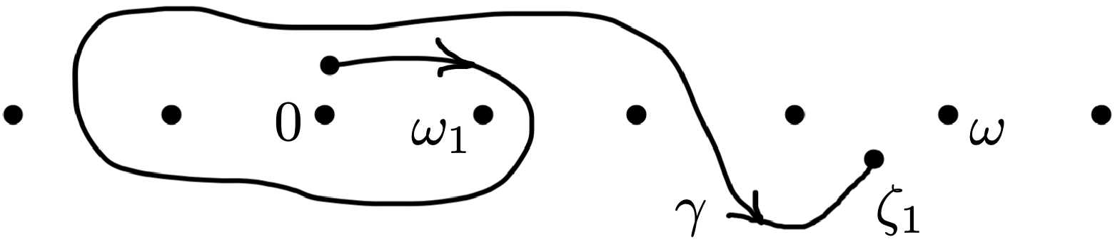
Figure 1: The path $\gamma$ avoids $\Omega$ and ends at ${\zeta}_{1}$, near $\omega$.

Defining

$$\mathscr{B}\colon\thinspace\mathbb{C}[[z^{-1}]]\to\mathbb{C}\,\delta\oplus\mathbb{C}[[{\zeta}]],\qquad\mathscr{B}\widetilde{\varphi}\coloneqq c_{0}\,\delta+\widehat{\varphi}$$ (5)

(here $\delta$ is just a symbol representing the image of $1$), we have

$$\mathbb{C}\{z^{-1}\}\subset\widetilde{\mathcal{R}}\,\!^{\mathrm{s}}_{\Omega}=\mathscr{B}^{-1}\big{(}\widehat{\mathcal{R}}\,\!^{\mathrm{s}}_{\Omega}\big{)}\subset\mathbb{C}[[z^{-1}]]$$ (6)

with $\widehat{\mathcal{R}}\,\!^{\mathrm{s}}_{\Omega}\coloneqq$ the set of all $c_{0}\,\delta+\widehat{\varphi}\in\mathbb{C}\,\delta\oplus\mathbb{C}\{{\zeta}\}$ such that $\widehat{\varphi}$ extends analytically to the universal cover of $\mathbb{C}-\Omega$ and has at worst simple singularities.

The first inclusion in (6) means that convergent series are always resurgent: if the radius of convergence of $\widetilde{\varphi}(z)$ happens to be positive, then $\widehat{\varphi}({\zeta})$ extends to an entire function of ${\zeta}$, thus the above definition is satisfied with any $\Omega$.

Examples of divergent simple $\Omega$-resurgent series. The Euler series $\widetilde{\varphi}^{\raisebox{-0.69318pt}{$\scriptstyle\mathrm{E}$}}(z)\coloneqq\sum_{p\geq 0}(-1)^{p}p!z^{-p-1}$ (formal solution to the equation $-\frac{{\mathrm{d}}\varphi}{{\mathrm{d}}z}+\varphi=z^{-1}$) and the Stirling series $\widetilde{\varphi}^{\raisebox{-0.69318pt}{$\scriptstyle\mathrm{S}$}}(z)\coloneqq\frac{1}{12}z^{-1}-\frac{1}{360}z^{-3}+\frac{1}{1260}z^{-5}+\cdots$ (asymptotic expansion of $\log\big{(}\frac{1}{\sqrt{2\pi}}z^{\frac{1}{2}-z}\mathrm{e}^{z}{\Gamma}(z)\big{)}$ as $\lvert z\rvert\to\infty$ with $\lvert\arg z\rvert\leq\pi-{\varepsilon}$) have Borel transforms

$$\widehat{\varphi}^{\raisebox{-0.69318pt}{$\scriptstyle\mathrm{E}$}}({\zeta})=\frac{1}{1+{\zeta}},\qquad\widehat{\varphi}^{\raisebox{-0.69318pt}{$\scriptstyle\mathrm{S}$}}({\zeta})={\zeta}^{-2}\Big{(}\frac{{\zeta}}{2}\coth\frac{{\zeta}}{2}-1\Big{)}$$ (7)

meromorphic with simple poles in $\Omega=\mathbb{Z}$ or $2\pi{\mathrm{i}}\mathbb{Z}$. But the typical Borel transforms found in practice are multivalued, as is the case for instance for $\exp(\widetilde{\varphi}^{\raisebox{-0.69318pt}{$\scriptstyle\mathrm{S}$}}(z))\in\widetilde{\mathcal{R}}\,\!^{\mathrm{s}}_{2\pi{\mathrm{i}}\mathbb{Z}}$ (asymptotic expansion of $\frac{1}{\sqrt{2\pi}}z^{\frac{1}{2}-z}\mathrm{e}^{z}{\Gamma}(z)$), whose Borel transform can be expressed in terms of the Lambert $W$ function [Sau21]. In the latter example, the Borel transform has a principal branch regular at ${\zeta}=0$ but the other branches of its analytic continuation are singular at $0$. A more elementary example of the same phenomenon is offered by $\operatorname{Li}_{2}({\zeta})\coloneqq-\int_{0}^{\zeta}\log(1-\xi)\frac{{\mathrm{d}}\xi}{\xi}\in\widehat{\mathcal{R}}\,\!^{\mathrm{s}}_{\mathbb{Z}}$.

The growth of the coefficients of a resurgent series $\widetilde{\varphi}(z)$ is at most factorial, because $\mathscr{B}\widetilde{\varphi}\in\mathbb{C}\,\delta\oplus\mathbb{C}\{{\zeta}\}$ implies that there exist $C,M>0$ such that $\lvert c_{n}\rvert\leq CM^{n}n!$. Such series are said to be $1$-Gevrey. If the radius of convergence of $\widetilde{\varphi}(z)$ is zero, we may hope to get information on its divergence by studying the singularities of its Borel transform. This will be done by means of Écalle’s alien operators (see below).

2.2 Stability under product and nonlinear operations

It is obvious that $\widetilde{\mathcal{R}}\,\!^{\mathrm{s}}_{\Omega}$ is a $\mathbb{C}$-vector space stable under $\frac{{\mathrm{d}}\;}{{\mathrm{d}}z}$ (note that $\mathscr{B}$ maps differentiation to multiplication by $-{\zeta}$). Much less obviously, it is also stable under multiplication and is thus a subalgebra of $\mathbb{C}[[z^{-1}]]$. This is due to the compatibility of the process of analytic continuation with the convolution

$$\widehat{\varphi}*\widehat{\psi}({\zeta})\coloneqq\int_{0}^{\zeta}\widehat{\varphi}(u)\widehat{\psi}({\zeta}-u)\,{\mathrm{d}}u$$ (8)

and to the fact that $\mathscr{B}$ maps the standard (Cauchy) product of formal series $\widetilde{\varphi}\,\widetilde{\psi}$ to $\mathscr{B}\widetilde{\varphi}*\mathscr{B}\widetilde{\psi}$, where $\delta=\mathscr{B}1$ is a unit for the convolution: one can indeed check that, because $\Omega$ is stable under addition, the space $\widehat{\mathcal{R}}\,\!^{\mathrm{s}}_{\Omega}$ is stable under convolution [Éca81, CNP93, Sau13].

The algebra $\widetilde{\mathcal{R}}\,\!^{\mathrm{s}}_{\Omega}$ is also stable under nonlinear operations like substitution into a convergent series, or composition of the form $\widetilde{\varphi}\circ(\mathop{\hbox{{\rm Id}}}\nolimits+\widetilde{\psi})$. For instance, the exponential of any simple $\Omega$-resurgent series and—if it has nonzero constant term—its multiplicative inverse are simple $\Omega$-resurgent series; also, $\{\mathop{\hbox{{\rm Id}}}\nolimits+\widetilde{\psi}\mid\widetilde{\psi}\in\widetilde{\mathcal{R}}\,\!^{\mathrm{s}}_{\Omega}\}$ is a group for composition [Éca81] (see [Sau15] for explicit estimates in the Borel plane that allow one to prove these stability properties).

2.3 Alien operators. Alien derivations

Notice that in (4), the regular part $F$ depends on the choice of the branch of the logarithm, whereas $a_{0}$ and $\widehat{\chi}$ are uniquely determined. Thus, for $\gamma$ and $\omega$ as above, we can use the formula

$$\mathscr{A}_{\omega}^{\gamma}\widetilde{\varphi}\coloneqq\mathscr{B}^{-1}(a_{0}\,\delta+\widehat{\chi})$$ (9)

to define a $\mathbb{C}$-linear operator $\mathscr{A}_{\omega}^{\gamma}$, which clearly maps $\widetilde{\mathcal{R}}\,\!^{\mathrm{s}}_{\Omega}$ to itself (because $\Omega$ is an additive group and $\widehat{\chi}$, being the difference of two branches of $\widehat{\varphi}$ translated by $\omega$, must belong to $\widehat{\mathcal{R}}\,\!^{\mathrm{s}}_{\Omega}$).

We call alien operators of $\widetilde{\mathcal{R}}\,\!^{\mathrm{s}}_{\Omega}$ the elements of the subalgebra of $\operatorname{End}_{\mathbb{C}}\!\big{(}\widetilde{\mathcal{R}}\,\!^{\mathrm{s}}_{\Omega}\big{)}$ generated by the $\mathscr{A}_{\omega}^{\gamma}$’s. Note that they all annihilate convergent series, since $\mathbb{C}\{z^{-1}\}\subset\ker(\mathscr{A}_{\omega}^{\gamma})$. Among them, we single out two families of operators, $(\Delta_{\omega}^{+})_{\omega\in\Omega^{+}}$ and $(\Delta_{\omega})_{\omega\in\Omega^{+}}$, where

$$\Omega^{+}\coloneqq\{\omega_{k}\mid k\in\mathbb{Z}_{>0}\}$$ (10)

with reference to (2).

Definition 2.

Let $\omega=\omega_{r}\in\Omega^{+}$ ($r\in\mathbb{Z}_{>0}$). We consider, for each ${\varepsilon}=({\varepsilon}_{1},\ldots,{\varepsilon}_{r-1})\in\{+,-\}^{r-1}$, the path $\gamma({\varepsilon})$ that connects $\delta\omega_{1}\in\,]0,\omega_{1}[$, where $\delta\in(0,\frac{1}{2})$, to $(r-\delta)\omega_{1}\in\,]\omega_{r-1},\omega[$ by following $]0,\omega[$ except that $\omega_{k}$ is circumvented to the right (resp. left) if ${\varepsilon}_{k}=+$ (resp. $-$). See Fig. 2. We set

$$\Delta^{+}_{\omega}\coloneqq\mathscr{A}_{\omega}^{\gamma(+,\ldots,+)},\enspace\Delta_{\omega}\coloneqq\sum_{{\varepsilon}\in\{+,-\}^{r-1}}\frac{p({\varepsilon})!q({\varepsilon})!}{r!}\mathscr{A}_{\omega}^{\gamma({\varepsilon})},$$ (11)

where $p({\varepsilon})$ and $q({\varepsilon})=r-1-p({\varepsilon})$ are the numbers of symbols ‘$+$’ and ‘$-$’ in the tuple ${\varepsilon}$.

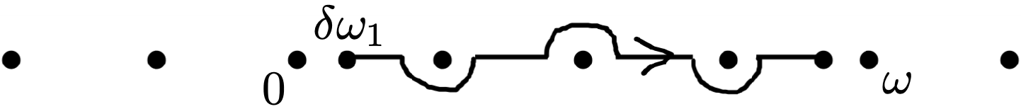
Figure 2: An example of path $\gamma({\varepsilon})$, here with $r=4$ and ${\varepsilon}=(+,-,+)$.

The weights used in (11) for the second family have been chosen so that these operators satisfy the Leibniz product rule, for which reason $\Delta_{\omega}$ is called the alien derivation with index $\omega$.

Theorem 3 ([Éca81]).

For each $\omega\in\Omega^{+}$, the operator $\Delta_{\omega}$ is a derivation of the algebra $\widetilde{\mathcal{R}}\,\!^{\mathrm{s}}_{\Omega}$.

There is even an ‘alien chain rule’. For instance, for the Stirling series, $\Delta_{\omega}\big{(}\mathrm{e}^{\widetilde{\varphi}^{\raisebox{-0.49512pt}{$\scriptscriptstyle\mathrm{S}$}}}\big{)}=(\Delta_{\omega}\widetilde{\varphi}^{\raisebox{-0.69318pt}{$\scriptstyle\mathrm{S}$}})\mathrm{e}^{\widetilde{\varphi}^{\raisebox{-0.49512pt}{$\scriptscriptstyle\mathrm{S}$}}}$, with $\Delta_{\omega}\widetilde{\varphi}^{\raisebox{-0.69318pt}{$\scriptstyle\mathrm{S}$}}=1/r$ if $\omega=2\pi{\mathrm{i}}r$.

One way of proving Theorem 3 is to check that one can express $\Delta_{\omega_{r}}$ in terms of $\Delta^{+}_{\omega_{1}},\ldots,\Delta^{+}_{\omega_{r}}$ and that each $\Delta^{+}_{\omega}$ satisfies a modified Leibniz rule:

$$\Delta^{+}_{\omega_{r}}(\widetilde{\varphi}\,\widetilde{\psi})=(\Delta^{+}_{\omega_{r}}\widetilde{\varphi})\,\widetilde{\psi}+\sum_{k=1}^{r-1}(\Delta^{+}_{\omega_{r-k}}\widetilde{\varphi})\Delta^{+}_{\omega_{k}}\,\widetilde{\psi}+\widetilde{\varphi}\Delta^{+}_{\omega_{r}}\,\widetilde{\psi}.$$ (12)

A more conceptual explanation stems from the relation of these operators to the symbolic Stokes automorphism described in Section 3.2 below.

Let $\Omega^{-}\coloneqq\{-k\omega_{1}\mid k\in\mathbb{Z}_{>0}\}$. By repeating the previous definitions with $\omega_{1}$ changed into $-\omega_{1}$, we get alien operators $\Delta^{+}_{\omega}$ and alien derivations $\Delta_{\omega}$ for all $\omega\in\Omega^{\prime}\coloneqq\Omega-\{0\}$.

Large $n$ asymptotics of the $c_{n}$’s. Notice that, for a given $\widetilde{\varphi}(z)=\sum_{n\geq 0}c_{n}z^{-n}\in\widetilde{\mathcal{R}}\,\!^{\mathrm{s}}_{\Omega}$, since the $c_{n}$’s appear as coefficients in the Taylor expansion of $\widehat{\varphi}({\zeta})$ which has $\pm\omega_{1}$ as its nearest-to-origin potential singular points, their growth is dictated by the nature of the singularities there, i.e. by $\Delta_{\omega_{\pm 1}}\widetilde{\varphi}=\Delta^{+}_{\omega_{\pm 1}}\widetilde{\varphi}$. For instance, denoting by $a_{\pm}$ the constant term in $\Delta^{+}_{\omega_{\pm 1}}\widetilde{\varphi}$, one can prove that

$$c_{n+1}=-\frac{1}{2\pi{\mathrm{i}}}n!\big{(}\omega_{1}^{-n-1}a_{+}+\omega_{-1}^{-n-1}a_{-}+O(\lvert\omega_{1}\rvert^{-n}n^{-1})\big{)}$$ (13)

and one can refine this estimate to arbitrary precision by using later terms in $\Delta^{+}_{\pm\omega_{1}}\widetilde{\varphi}$, and even get a transasymptotic expansion (involving corrections of orders $\omega_{\pm 2}^{-n},\omega_{\pm 3}^{-n},\ldots$) by incorporating contributions from $\Delta^{+}_{\pm\omega_{2}}\widetilde{\varphi},\Delta^{+}_{\pm\omega_{3}}\widetilde{\varphi},\ldots$

2.4 Freeness of the alien derivations and a first glimpse of mould calculus

The term ‘alien derivation’ was coined by [Éca81] to highlight how this array of operators is different in nature from the natural derivation $\frac{{\mathrm{d}}\;}{{\mathrm{d}}z}$. If we focus on $\operatorname{Der}_{\mathbb{C}}(\widetilde{\mathcal{R}}\,\!^{\mathrm{s}}_{\Omega})$, viewed as a Lie subalgebra of $\operatorname{End}_{\mathbb{C}}(\widetilde{\mathcal{R}}\,\!^{\mathrm{s}}_{\Omega})$ with commutator as Lie bracket, we have the relation

$$\big{[}\tfrac{{\mathrm{d}}\;}{{\mathrm{d}}z},\Delta_{\omega}\big{]}=\omega\Delta_{\omega}\quad\text{for each $\omega\in\Omega^{\prime}$}$$ (14)

(easy to check from the definition), but the striking fact is that the Lie subalgebra generated by $(\Delta_{\omega})_{\omega\in\Omega^{\prime}}$ under Lie bracketing and multiplication by arbitrary elements of $\widetilde{\mathcal{R}}\,\!^{\mathrm{s}}_{\Omega}$ is isomorphic to the tensor product of $\widetilde{\mathcal{R}}\,\!^{\mathrm{s}}_{\Omega}$ with the free Lie algebra over $\Omega^{\prime}=\Omega-\{0\}$. We thus have, in this very analytic context, an infinite-dimensional free Lie algebra! This is in marked contrast with $\mathbb{C}[[z^{-1}]]$, all of whose derivations are generated by $\tfrac{{\mathrm{d}}\;}{{\mathrm{d}}z}$, i.e. of the form $\alpha(z)\tfrac{{\mathrm{d}}\;}{{\mathrm{d}}z}$, $\alpha\in\mathbb{C}[[z^{-1}]]$.

We can also consider the associative subalgebra of $\operatorname{End}_{\mathbb{C}}(\widetilde{\mathcal{R}}\,\!^{\mathrm{s}}_{\Omega})$ generated by the $\Delta_{\omega}$’s, and there is a similar statement. Formulating precisely these facts will usher us into the realm of mould calculus.

From now on we relinquish the notations ‘$\omega_{1}$’ and ‘$\omega_{k}$’ of (2) and use $\omega_{1},\ldots,\omega_{r}$ to denote generic elements of $\Omega^{\prime}$. In fact, we will view $\Omega^{\prime}$ as an alphabet, whose letters form words ${\underline{\omega}}=\omega_{1}\cdots\omega_{r}$ (with arbitrary $\omega_{1},\ldots,\omega_{r}\in\Omega^{\prime}$ and $r\in\mathbb{Z}_{\geq 0}$, including the empty word ${\varnothing}$ in the case $r=0$). We denote by ${\underline{\Omega\hskip 0.50003pt}^{\prime}}$ the set of all words on $\Omega^{\prime}$.

Theorem 4 ([Éca81]).

Let

$$\Delta_{\underline{\omega}}\coloneqq\Delta_{\omega_{r}}\cdots\Delta_{\omega_{1}}\enspace\text{for any ${\underline{\omega}}=\omega_{1}\cdots\omega_{r}\in{\underline{\Omega\hskip 0.50003pt}^{\prime}}$,}$$ (15)

with the convention $\Delta_{\varnothing}\coloneqq\mathop{\hbox{{\rm Id}}}\nolimits$. Consider, for any finitely-supported family $\Phi=(\Phi^{{\underline{\omega}}})_{{\underline{\omega}}\in{\underline{\Omega\hskip 0.35002pt}^{\prime}}}$ of elements of $\widetilde{\mathcal{R}}\,\!^{\mathrm{s}}_{\Omega}$, the operator

$$\Phi{{\Delta}}\raisebox{1.59302pt}{\leavevmode\resizebox{2.58334pt}{}{$\mathrm{/}$}}\hskip 3.43254pt{}\coloneqq\sum_{{\underline{\omega}}\in{\underline{\Omega\hskip 0.35002pt}^{\prime}}}\Phi^{\underline{\omega}}\Delta_{\underline{\omega}}\in\operatorname{End}_{\mathbb{C}}(\widetilde{\mathcal{R}}\,\!^{\mathrm{s}}_{\Omega}).$$ (16)

Then $\Phi{{\Delta}}\raisebox{1.59302pt}{\leavevmode\resizebox{2.58334pt}{}{$\mathrm{/}$}}\hskip 3.43254pt{}$ is nonzero, unless all coefficients $\Phi^{\underline{\omega}}$ are zero.

For instance, $\Delta_{\omega_{1}}\Delta_{\omega_{2}}$ is a non-trivial operator for any $\omega_{1},\omega_{2}\in\Omega^{\prime}$, and $\Delta_{\omega_{1}}\Delta_{\omega_{2}}-\Delta_{\omega_{2}}\Delta_{\omega_{1}}$ is a non-trivial derivation if $\omega_{1}\neq\omega_{2}$.

In a formula like (16), the family $\Phi=(\Phi^{{\underline{\omega}}})_{{\underline{\omega}}\in{\underline{\Omega\hskip 0.35002pt}^{\prime}}}$ is called an $\widetilde{\mathcal{R}}\,\!^{\mathrm{s}}_{\Omega}$-valued mould, and the right-hand side is called a mould expansion—see Section 5 on Mould Calculus below. Here, the finite support condition is needed to make sense of the summation, but later in Section 5 we will consider moulds that are not necessarily finitely-supported and take their values in an arbitrary commutative algebra, not necessarily $\widetilde{\mathcal{R}}\,\!^{\mathrm{s}}_{\Omega}$.

The proof of Theorem 4 follows from Theorem 10 given in Section 5. The idea is that, according to Theorem 10, there is an $\widetilde{\mathcal{R}}\,\!^{\mathrm{s}}_{\Omega}$-valued mould $(\mathscr{U}^{{\underline{\omega}}})_{{\underline{\omega}}\in{\underline{\Omega\hskip 0.35002pt}^{\prime}}}$ such that $\mathscr{U}^{\varnothing}=1$ and, for every $\omega_{0}\in\Omega^{\prime}$ and ${\underline{\omega}}=\omega_{1}\cdots\omega_{r}\in{\underline{\Omega\hskip 0.50003pt}^{\prime}}$,

$$\Delta_{\omega_{0}}\mathscr{U}^{\omega_{1}\cdots\omega_{r}}=\begin{cases}\mathscr{U}^{\omega_{2}\cdots\omega_{r}}&\text{if $r\geq 1$ and $\omega_{0}=\omega_{1}$}\\[4.30554pt] 0&\text{otherwise}.\end{cases}$$ (17)

Notice then that the support of $(\mathscr{U}^{{\underline{\omega}}})_{{\underline{\omega}}\in{\underline{\Omega\hskip 0.35002pt}^{\prime}}}$ must be all of ${\underline{\Omega\hskip 0.50003pt}^{\prime}}$ because $\Delta_{\omega_{r}}\cdots\Delta_{\omega_{1}}\mathscr{U}^{\omega_{1}\cdots\omega_{r}}=\mathscr{U}^{\varnothing}\neq 0$. More generally, for any ${\underline{a}}\in{\underline{\Omega\hskip 0.50003pt}^{\prime}}$,

$$\Delta_{\underline{a}}\mathscr{U}^{{\underline{\omega}}}=\begin{cases}0&\text{if ${\underline{a}}$ is not a prefix of ${\underline{\omega}}$}\\[4.30554pt] \mathscr{U}^{\underline{b}}&\text{if ${\underline{\omega}}={\underline{a}}\,{\underline{b}}$},\end{cases}$$ (18)

which easily implies Theorem 4 since it gives $(\Phi{{\Delta}}\raisebox{1.59302pt}{\leavevmode\resizebox{2.58334pt}{}{$\mathrm{/}$}}\hskip 3.43254pt{})\mathscr{U}^{{\underline{\omega}}^{*}}=\Phi^{{\underline{\omega}}^{*}}$ for any ${\underline{\omega}}^{*}$ of minimal length in the support of $\Phi$.

A mould $\Phi$ is called alternal if

$$\Phi^{\varnothing}=0\enspace\text{and}\enspace\sum_{{\underline{\omega}}\in{\underline{\Omega\hskip 0.35002pt}^{\prime}}}\operatorname{sh}\!\big{(}\begin{smallmatrix}{\underline{a}},\,{\underline{b}}\\ {\underline{\omega}}\end{smallmatrix}\big{)}\Phi^{{\underline{\omega}}}=0\;\text{for any}\ {\underline{a}},{\underline{b}}\neq{\varnothing},$$ (19)

where the ‘shuffling’ coefficient $\operatorname{sh}\!\big{(}\begin{smallmatrix}{\underline{a}},\,{\underline{b}}\\ {\underline{\omega}}\end{smallmatrix}\big{)}$ counts the number of permutations that allow to interdigitate the letters of ${\underline{a}}$ and ${\underline{b}}$ so as to obtain ${\underline{\omega}}$ while preserving their internal order in ${\underline{a}}$ or ${\underline{b}}$. For instance, the condition (19) with ${\underline{a}}=\omega_{1}$ and ${\underline{b}}=\omega_{2}$ says that $\Phi^{\omega_{1}\omega_{2}}+\Phi^{\omega_{2}\omega_{1}}=0$ and, with ${\underline{a}}=\omega_{1}$ and ${\underline{b}}=\omega_{1}\omega_{2}$, that $2\Phi^{\omega_{1}\omega_{1}\omega_{2}}+\Phi^{\omega_{1}\omega_{2}\omega_{1}}=0$.

We shall say more on alternality and related mould symmetries in Section 5, but let us already mention that one interest of alternal moulds lies in the following

Proposition 5.

For any alternal $\widetilde{\mathcal{R}}\,\!^{\mathrm{s}}_{\Omega}$-valued mould $(\Phi^{\underline{\omega}})_{{\underline{\omega}}\in{\underline{\Omega\hskip 0.35002pt}^{\prime}}}$, the operator (16) satisfies

$$\Phi{{\Delta}}\raisebox{1.59302pt}{\leavevmode\resizebox{2.58334pt}{}{$\mathrm{/}$}}\hskip 3.43254pt{}=\sum_{{\underline{\omega}}\in{\underline{\Omega\hskip 0.35002pt}^{\prime}}}\Phi^{\underline{\omega}}\Delta_{\underline{\omega}}=\sum_{{\underline{\omega}}\in{\underline{\Omega\hskip 0.35002pt}^{\prime}}-\{{\varnothing}\}}\tfrac{1}{r({\underline{\omega}})}\Phi^{\underline{\omega}}\Delta_{[{\underline{\omega}}]}$$ (20)

where $r({\underline{\omega}})$ denotes the length of the word ${\underline{\omega}}$ and

$$\Delta_{[{\underline{\omega}}]}\coloneqq[\Delta_{\omega_{r}},[\ldots[\Delta_{\omega_{2}},\Delta_{\omega_{1}}]\ldots]]\quad\text{for ${\underline{\omega}}=\omega_{1}\cdots\omega_{r}$}$$ (21)

(with the convention $\Delta_{[\omega_{1}]}=\Delta_{\omega_{1}}$ if $r=1$). In particular, this alien operator is a derivation:

$$\text{$\Phi$ alternal}\quad\Rightarrow\quad\Phi{{\Delta}}\raisebox{1.59302pt}{\leavevmode\resizebox{2.58334pt}{}{$\mathrm{/}$}}\hskip 3.43254pt{}=\sum_{{\underline{\omega}}\in{\underline{\Omega\hskip 0.35002pt}^{\prime}}}\Phi^{\underline{\omega}}\Delta_{\underline{\omega}}\in\operatorname{Der}_{\mathbb{C}}(\widetilde{\mathcal{R}}\,\!^{\mathrm{s}}_{\Omega}).$$ (22)

Thus, in view of Theorem 4, when dealing with operators of the form (20), i.e. in the alternal case, we are actually working in the free Lie algebra on $\Omega^{\prime}$ (but we use an indexation by all the words and restrict to coefficients given by alternal moulds, instead of using a Lyndon basis or a Hall basis).

3 Simple resurgent functions obtained by Borel-Laplace summation

3.1 Borel-Laplace summation

Many resurgent series encountered in practice are useful because they are also ‘summable’ (or ‘accelero-summable’, but we won’t touch on accelero-summability in this article).

Borel-Laplace summation is the application of Laplace transform (or some variant) to $(\mathscr{B}\widetilde{\varphi})({\zeta})$, giving rise to a function $\varphi(z)$ for which the formal series $\widetilde{\varphi}(z)$ appears as asymptotic expansion at infinity; but the function $\varphi$ is usually not analytic in a full neighbourhood of infinity, only in a sectorial neighbourhood, because $\widetilde{\varphi}$ is usually a divergent series.

A condition is needed for this to be possible. Let $J$ denote a real interval. We say that $\widetilde{\varphi}(z)$ is $1$-summable in the directions of $J$ if the function $\widehat{\varphi}({\zeta})$ extends analytically to the sector $\{\arg{\zeta}\in J\}$ and satisfies there an exponential bound, $\lvert\widehat{\varphi}({\zeta})\rvert\leq C\,\mathrm{e}^{c\lvert{\zeta}\rvert}$ for some $c,C>0$. Each of the Laplace transforms

$$(\mathscr{L}^{\theta}\!\mathscr{B}\widetilde{\varphi})(z)\coloneqq c_{0}+\int_{0}^{\mathrm{e}^{{\mathrm{i}}{\theta}}\infty}\mathrm{e}^{-z{\zeta}}\,\widehat{\varphi}({\zeta})\,{\mathrm{d}}{\zeta},\qquad{\theta}\in J$$ (23)

is then analytic in the half-plane $\{\mathop{\Re e}\nolimits(z\mathrm{e}^{{\mathrm{i}}{\theta}})>c\}$. By the Cauchy theorem, these functions match and can be glued so as to define one function $(\mathscr{L}^{J}\!\mathscr{B}\widetilde{\varphi})(z)$ analytic in the union $\mathscr{D}^{J}$ of these half-planes—see Figure 3. The domain $\mathscr{D}^{J}$ can be viewed as a sectorial neighbourhood of infinity of opening $\lvert J\rvert+\pi$ (to be considered as a part of the Riemann surface of the logarithm if $\lvert J\rvert>\pi$).

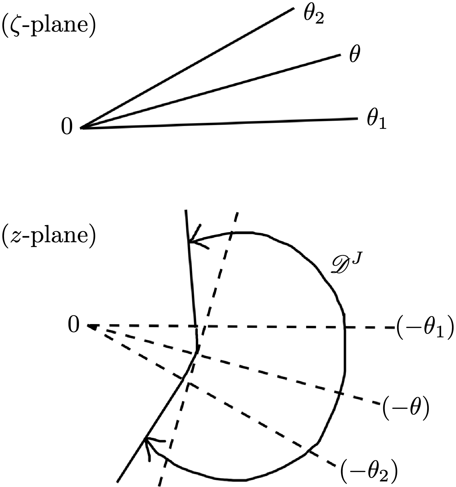
Figure 3: Above: Directions for Laplace integration with $J=({\theta}_{1},{\theta}_{2})$. Below: the union of half-planes $\mathscr{D}^{J}$.

In that situation, the function $\mathscr{S}^{J}\widetilde{\varphi}\coloneqq\mathscr{L}^{J}\!\mathscr{B}\widetilde{\varphi}$ satisfies the asymptotic property $(\mathscr{S}^{J}\widetilde{\varphi})(z)\sim\widetilde{\varphi}(z)$ as $\lvert z\rvert\to\infty$ with $1$-Gevrey qualification—a classical fact that sometimes goes under the name of Watson’s lemma, see e.g. [Cos09, MS16]. The operator

$$\mathscr{S}^{J}=\mathscr{L}^{J}\circ\mathscr{B}$$ (24)

is thus called the Borel-Laplace summation operator in the directions of $J$. One can easily check that

$$\mathscr{S}^{J}\tfrac{{\mathrm{d}}\widetilde{\varphi}}{{\mathrm{d}}z}=\tfrac{{\mathrm{d}}\;}{{\mathrm{d}}z}(\mathscr{S}^{J}\widetilde{\varphi})\;\text{and}\;\mathscr{S}^{J}\!\big{[}\widetilde{\varphi}(z+\alpha)\big{]}=(\mathscr{S}^{J}\widetilde{\varphi})(z+\alpha)$$ (25)

for any $\alpha\in\mathbb{C}$. The summation operator is also an algebra homomorphism. Indeed, $\mathscr{B}$ maps the Cauchy product of formal series to convolution in $\mathbb{C}\,\delta\oplus\mathbb{C}\{{\zeta}\}$, which $\mathscr{L}^{J}$ maps to the pointwise product of functions:

$$\mathscr{S}^{J}(\widetilde{\varphi}\,\widetilde{\psi})=(\mathscr{S}^{J}\widetilde{\varphi})(\mathscr{S}^{J}\widetilde{\psi}).$$ (26)

Equations (25)–(26) show that, if we start with $\widetilde{\varphi}(z)$ formal solution to an ordinary differential equation or a difference equation, even a nonlinear one, and if we can subject it to Borel-Laplace summation, then $\mathscr{S}^{J}\widetilde{\varphi}(z)$ is an analytic solution to the same equation. Notice however that there may exist other solutions with the same asymptotic series $\widetilde{\varphi}$, maybe obtained by means of $\mathscr{S}^{J^{\prime}}$ with a different interval $J^{\prime}$, or by some other means…

The Borel-Laplace picture becomes particularly interesting when we start with a resurgent series $\widetilde{\varphi}(z)$, in which case $\varphi^{J}(z)\coloneqq\mathscr{S}^{J}\widetilde{\varphi}(z)$ deserves to be called a resurgent function.

3.2 Transseries, symbolic Stokes automorphism

Indeed, let us pick a generator $\omega_{1}$ of $\Omega$ and ${\theta}_{*}\in\mathbb{R}$ so that $\Omega^{+}\subset d\coloneqq\mathrm{e}^{{\mathrm{i}}{\theta}_{*}}\mathbb{R}_{>0}$ (making use of notations (2) and (10)). Suppose that $\widetilde{\varphi}\in\widetilde{\mathcal{R}}\,\!^{\mathrm{s}}_{\Omega}$ is $1$-summable in the directions of $J_{+}\coloneqq({\theta}_{*}-\delta,{\theta}_{*})$ as well as those of $J_{-}\coloneqq({\theta}_{*},{\theta}_{*}+\delta)$ for some $\delta\in(0,\pi)$. We then have two Borel sums at our disposal, $\mathscr{S}^{J_{+}}\widetilde{\varphi}(z)$ and $\mathscr{S}^{J_{-}}\widetilde{\varphi}(z)$. Comparing them in the domain $\mathscr{D}^{J_{+}}\cap\mathscr{D}^{J_{-}}\cap\{\mathop{\Re e}\nolimits(z\mathrm{e}^{{\mathrm{i}}{\theta}_{*}})>0\}$, we find

$$\mathscr{S}^{J_{+}}\widetilde{\varphi}(z)-\mathscr{S}^{J_{-}}\widetilde{\varphi}(z)=\int_{{\Gamma}_{\!\textrm{diff}}}\!\mathrm{e}^{-z{\zeta}}\,\widehat{\varphi}({\zeta})\,{\mathrm{d}}{\zeta}$$ (27)

with a contour ${\Gamma}_{\!\textrm{diff}}$ that can be decomposed in a sum of contours ${\Gamma}_{1},{\Gamma}_{2},\ldots$ as illustrated on Figure (4).

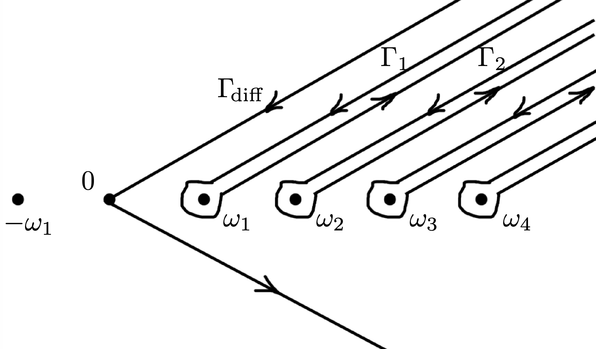
Figure 4: Decomposition of the contour for the difference of two Laplace transforms as a sum of contours.

By the Cauchy theorem we thus get

$$\mathscr{S}^{J_{+}}\widetilde{\varphi}(z)=\mathscr{S}^{J_{-}}\widetilde{\varphi}(z)+\sum_{k\geq 1}\int_{{\Gamma}_{k}}\mathrm{e}^{-z{\zeta}}\,\widehat{\varphi}({\zeta})\,{\mathrm{d}}{\zeta},$$ (28)

at least if the growth of the relevant branches of $\widehat{\varphi}({\zeta})$ along the ${\Gamma}_{k}$’s stays at most exponential and the series over $k$ is convergent (if not, (28) still has asymptotic meaning upon appropriate truncations). The point is that, for each $k\geq 1$, in view of (4), (9) and (11), the branch of $\widehat{\varphi}({\zeta})$ that we are using along ${\Gamma}_{k}$ has a pole and a monodromy variation precisely described by $\mathscr{B}\Delta^{+}_{\omega_{k}}\widetilde{\varphi}$, hence

$$\int_{{\Gamma}_{k}}\mathrm{e}^{-z{\zeta}}\,\widehat{\varphi}({\zeta})\,{\mathrm{d}}{\zeta}=\mathrm{e}^{-\omega_{k}z}\mathscr{S}^{J_{-}}\Delta^{+}_{\omega_{k}}\widetilde{\varphi}(z)$$ (29)

(use the change of variable ${\zeta}=\omega_{k}+\xi$ and (40)–(41) below) and, finally,

$$\mathscr{S}^{J_{+}}\widetilde{\varphi}=\mathscr{S}^{J_{-}}\widetilde{\varphi}+\sum_{k\geq 1}\mathrm{e}^{-\omega_{k}z}\mathscr{S}^{J_{-}}\Delta^{+}_{\omega_{k}}\widetilde{\varphi}.$$ (30)

The right-hand side of (30) can be interpreted as the Borel-Laplace summation of a transseries, i.e. we are naturally led to work with expressions of the form

$$\widetilde{\Psi}=\widetilde{\psi}_{0}+\sum_{k\geq 1}\mathrm{e}^{-\omega_{k}z}\widetilde{\psi}_{k},\qquad\widetilde{\psi}_{0},\widetilde{\psi}_{1},\widetilde{\psi}_{2}\ldots\in\widetilde{\mathcal{R}}\,\!^{\mathrm{s}}_{\Omega},$$ (31)

which live in the space

$$\widetilde{\mathcal{R}}\,\!^{\mathrm{s}}_{\Omega}[[\mathrm{e}^{-\omega_{1}z}]]=\underset{k\geq 0}{\widehat{\oplus}}\mathrm{e}^{-k\omega_{1}z}\widetilde{\mathcal{R}}\,\!^{\mathrm{s}}_{\Omega}.$$ (32)

We view that space as a completed graded algebra, in which acts the operator

$${{\Delta}}\raisebox{1.59302pt}{\leavevmode\resizebox{2.58334pt}{}{$\mathrm{/}$}}\hskip 3.43254pt{}^{+}_{d}\coloneqq\mathop{\hbox{{\rm Id}}}\nolimits+\sum_{\omega\in\Omega\cap d}\mathrm{e}^{-\omega z}\Delta^{+}_{\omega},$$ (33)

and to which we extend $\mathscr{S}^{J_{\pm}}$ by declaring that $\mathscr{S}^{J}[\mathrm{e}^{-\omega z}\widetilde{\Psi}]\coloneqq\mathrm{e}^{-\omega z}\mathscr{S}^{J}\widetilde{\Psi}$, the upshot being

$$\mathscr{S}^{J_{+}}=\mathscr{S}^{J_{-}}\circ{{\Delta}}\raisebox{1.59302pt}{\leavevmode\resizebox{2.58334pt}{}{$\mathrm{/}$}}\hskip 3.43254pt{}^{+}_{d},$$ (34)

at least in restriction to those transseries of $\widetilde{\mathcal{R}}\,\!^{\mathrm{s}}_{\Omega}[[\mathrm{e}^{-\omega_{1}z}]]$ all of whose components satisfy the growth and convergence requirements needed for (28).

We can now reach a more conceptual understanding of Theorem 3 and the identities (12):

• The identities (12) express that ${{\Delta}}\raisebox{1.59302pt}{\leavevmode\resizebox{2.58334pt}{}{$\mathrm{/}$}}\hskip 3.43254pt{}^{+}_{d}$ is an algebra endomorphism, which is no surprise since (34) involves two algebra homomorphisms $\mathscr{S}^{J_{\pm}}$.

• The formulas expressing $\Delta_{\omega_{r}}$ in terms of $\Delta^{+}_{\omega_{1}},\ldots,\Delta^{+}_{\omega_{r}}$ alluded to right after the statement of Theorem 3 are just the homogeneous components of the relation

  $$\log{{\Delta}}\raisebox{1.59302pt}{\leavevmode\resizebox{2.58334pt}{}{$\mathrm{/}$}}\hskip 3.43254pt{}^{+}_{d}=\sum_{\omega\in\Omega\cap d}\mathrm{e}^{-\omega z}\Delta_{\omega},$$ (35)

  which is the true origin of formula (11).

• In the context of a completed graded algebra like ours, the logarithm of an algebra automorphism is always a derivation, and the homogeneous components of a derivation are all derivations, this explains why each $\Delta_{\omega}$ is a derivation of $\widetilde{\mathcal{R}}\,\!^{\mathrm{s}}_{\Omega}$.

Definition 6.

The operator ${{\Delta}}\raisebox{1.59302pt}{\leavevmode\resizebox{2.58334pt}{}{$\mathrm{/}$}}\hskip 3.43254pt{}^{+}_{d}$ is called the symbolic Stokes automorphism in the direction $d=\mathrm{e}^{{\mathrm{i}}{\theta}_{*}}\mathbb{R}_{>0}$. The operator ${{\Delta}}\raisebox{1.59302pt}{\leavevmode\resizebox{2.58334pt}{}{$\mathrm{/}$}}\hskip 3.43254pt{}_{d}\coloneqq\log{{\Delta}}\raisebox{1.59302pt}{\leavevmode\resizebox{2.58334pt}{}{$\mathrm{/}$}}\hskip 3.43254pt{}^{+}_{d}$ is called the directional alien derivation in the direction $d$.

Here we see how we can go beyond the traditional theory of asymptotic series, in which a function is determined by its asymptotics only up to an infinitely flat function. In the framework of $1$-Gevrey asymptotics, flat functions are in fact exponentially small, and the previous computation offers a glimpse of how the resurgent tools gives us a handle on the exponentially small ambiguities inherent to the situation.

The point is that ${{\Delta}}\raisebox{1.59302pt}{\leavevmode\resizebox{2.58334pt}{}{$\mathrm{/}$}}\hskip 3.43254pt{}^{+}_{d}$ is an algebra automorphism that commutes with $\frac{{\mathrm{d}}\;}{{\mathrm{d}}z}$ and composition with $z\mapsto z+\alpha$, and thus preserves the property of being a formal solution to a differential or difference equation. One can construct other such automorphisms; the simplest example is $({{\Delta}}\raisebox{1.59302pt}{\leavevmode\resizebox{2.58334pt}{}{$\mathrm{/}$}}\hskip 3.43254pt{}^{+}_{d})^{w}$, with arbitrary $w\in\mathbb{C}$, which can be written as a mould expansion:

$$({{\Delta}}\raisebox{1.59302pt}{\leavevmode\resizebox{2.58334pt}{}{$\mathrm{/}$}}\hskip 3.43254pt{}^{+}_{d})^{w}=\sum_{{\underline{\omega}}\in{\underline{\Omega\hskip 0.35002pt}^{\prime}}}\tfrac{w^{r({\underline{\omega}})}}{r({\underline{\omega}})!}\mathrm{e}^{-\lVert{\underline{\omega}}\rVert z}\Delta_{\underline{\omega}}$$ (36)

with the notation $\lVert\omega_{1}\cdots\omega_{r}\rVert\coloneqq\omega_{1}+\cdots+\omega_{r}$. The case $w=\pm\frac{1}{2}$ gives rise to the median summation operator, $\mathscr{S}^{{\theta}_{*}}_{\operatorname{med}}\coloneqq\mathscr{S}^{J_{+}}\circ({{\Delta}}\raisebox{1.59302pt}{\leavevmode\resizebox{2.58334pt}{}{$\mathrm{/}$}}\hskip 3.43254pt{}^{+}_{d})^{-\frac{1}{2}}=\mathscr{S}^{J_{-}}\circ({{\Delta}}\raisebox{1.59302pt}{\leavevmode\resizebox{2.58334pt}{}{$\mathrm{/}$}}\hskip 3.43254pt{}^{+}_{d})^{\frac{1}{2}}$, especially useful when ${\theta}_{*}=0$ and real symmetry is at play.

All this can be particularly relevant in physics, where one often starts by developing a so-called perturbative theory, where various formal expansions naturally appear; but then, if they can be subjected to the resurgent apparatus, one may hope to incarnate them as functions with meaningful exponentially small contributions related to non-perturbative physics… This may be viewed as one striking success of Resurgence Theory: to give systematic mathematical tools allowing one to extract non-perturbative contributions from a perturbative divergent series, via the analysis of the singularities in the Borel plane, in line with the expectations of, for instance, [Par78] and ’t Hooft [Hoo79].

4 The algebra ${\stackrel{{\scriptstyle\raisebox{-0.69318pt}{$\scriptscriptstyle\bigtriangledown$}}}{{\mathcal{R}}}}$ of general resurgent singularities

We now relax one by one the two requirements imposed by Definition 1, namely that the only obstacles to analytic continuation may occur at points of a given lattice $\Omega$ and that the singularities are no worse than simple.

4.1 Relaxing the constraint on the location of singularities

Definition 7.

We call endlessly continuable any $\widehat{\varphi}({\zeta})$ analytic near $0$ for which, for every real $L>0$, there exists a finite subset $F_{L}$ of $\mathbb{C}$ such that $\widehat{\varphi}({\zeta})$ can be analytically continued along every Lipschitz path of length $<L$ starting in the initial domain of definition of $\widehat{\varphi}$ and avoiding $F_{L}$.

Variants are possible—see [CNP93, KS20], or [Éca85] for the most general definition (‘continuable with no cut’). The point is that singular points are possibly very numerous but, in a sense, still isolated. This leaves room for a behaviour such as the one envisioned by [Vor83a]: there may exist a dense subset $\Omega$ of $\mathbb{C}$ such that, at every point of $\Omega$, at least one of the branches of the analytic continuation of $\widehat{\varphi}$ is singular (but, in any given region of $\mathbb{C}$, one ‘sees’ only finitely many singularities at a time: you need longer and longer paths of analytic continuation to see more and more singularities in that region).

Denoting by $\widetilde{\mathcal{R}}\,\!^{\mathrm{s}}$ the space of all $\widetilde{\varphi}(z)\in\mathscr{B}^{-1}(\mathbb{C}\,\delta\oplus\mathbb{C}\{{\zeta}\})$ for which $\widehat{\varphi}({\zeta})$ is endlessly continuable with at worst simple singularities for all the branches of its analytic continuation, we can now define the alien operators

$$\Delta^{+}_{\omega}\in\operatorname{End}_{\mathbb{C}}(\widetilde{\mathcal{R}}\,\!^{\mathrm{s}}),\enspace\Delta_{\omega}\in\operatorname{Der}_{\mathbb{C}}(\widetilde{\mathcal{R}}\,\!^{\mathrm{s}}),\quad\text{for $\omega\in\mathbb{C}^{*}$}$$ (37)

as follows: given $\widetilde{\varphi}=\mathscr{B}^{-1}(\mathbb{C}\,\delta+\widehat{\varphi})\in\widetilde{\mathcal{R}}\,\!^{\mathrm{s}}$, Definition 7 allows us to find a finite subset of $]0,\omega[$, the points of which we denote by $\omega_{1}\prec\cdots\prec\omega_{r-1}$ (with reference to the natural total order on the line-segment), so that Definition 2 can be copied verbatim, except that the $\omega_{k}$’s do not necessarily lie on any lattice (take any $L>\lvert\omega\rvert$ and $\{\omega_{1},\ldots,\omega_{r-1}\}\coloneqq F_{L}\cap\,]0,\omega[$ in Definition 7).

Much of what has been said in the case of a lattice can be generalized to the case of $\widetilde{\mathcal{R}}\,\!^{\mathrm{s}}$; in particular, this is a differential subalgebra of $(\mathbb{C}[[z^{-1}]],\frac{{\mathrm{d}}\;}{{\mathrm{d}}z})$ and, in the summable case, we have a passage formula generalizing (33)–(35):

$$\mathscr{S}^{\{{\theta}\}}=\mathscr{S}^{\{{\theta}^{\prime}\}}\circ\bigg{(}\sum_{{\underline{\omega}}\in{\underline{\Omega\hskip 0.35002pt}^{\prime}}}P_{{\theta},{\theta}^{\prime}}^{\underline{\omega}}\,\mathrm{e}^{-\lVert{\underline{\omega}}\rVert z}\Delta_{\underline{\omega}}\bigg{)},\qquad{\theta}<{\theta}^{\prime},$$ (38)

(at least in restriction to the simple resurgent series for which the action of the right-hand side is well-defined), with a scalar mould $P_{{\theta},{\theta}^{\prime}}$ defined by

$$P_{{\theta},{\theta}^{\prime}}^{{\underline{\omega}}}\coloneqq\begin{cases}1&\text{if $r({\underline{\omega}})=0$}\\[4.30554pt] \frac{1}{r_{1}!\cdots r_{s}!}&\text{if ${\theta}<\arg\omega_{1}\leq\cdots\leq\arg\omega_{r}<{\theta}^{\prime}$}\\[4.30554pt] 0&\text{otherwise,}\end{cases}$$ (39)

where, in the second case, ${\underline{\omega}}=\omega_{1}\cdots\omega_{r}\neq{\varnothing}$, $s$ counts the number of pairwise distinct $\arg\omega_{j}$’s, and $r_{1},\ldots,r_{s}$ count their multiplicities ($r_{1}+\cdots+r_{s}=r$).

4.2 Relaxing the constraint on the nature of singularities

Our earlier computation of a difference of Laplace transforms illustrated by Figure 4 relied on the fact that, given a direction ${\theta}\in\mathbb{R}$, one has

$$a_{0}=\int_{\mathcal{H}_{\theta}}\mathrm{e}^{-z{\zeta}}\frac{a_{0}}{2\pi{\mathrm{i}}{\zeta}}\,{\mathrm{d}}{\zeta},\enspace(\mathscr{L}^{\theta}\widehat{\chi})(z)=\int_{\mathcal{H}_{\theta}}\mathrm{e}^{-z{\zeta}}\,\raisebox{-0.99025pt}{${\stackrel{{\scriptstyle\raisebox{-0.69318pt}{$\scriptscriptstyle\vee$}}}{{\chi}}}$}({\zeta})\,{\mathrm{d}}{\zeta},$$ (40)

where

$$\raisebox{-0.99025pt}{${\stackrel{{\scriptstyle\raisebox{-0.69318pt}{$\scriptscriptstyle\vee$}}}{{\chi}}}$}({\zeta})\coloneqq\widehat{\chi}({\zeta})\,\frac{\log{\zeta}}{2\pi{\mathrm{i}}}+F({\zeta}),\quad F({\zeta})\in\mathbb{C}\{{\zeta}\},$$ (41)

and $\mathcal{H}_{\theta}$ is a rotated Hankel contour as on Figure 5.

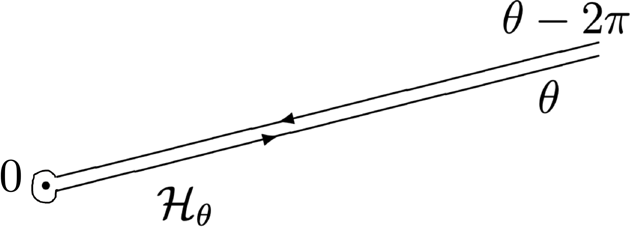
Figure 5: ${\theta}$-rotated Hankel contour.

Let us thus introduce the Hankel-type Laplace transform

$$(\raisebox{0.86108pt}{${\stackrel{{\scriptstyle\raisebox{-0.60275pt}{$\scriptscriptstyle\vee$}}}{{\mathscr{L}}}}$}\vphantom{\mathscr{L}}^{\theta}{\stackrel{{\scriptstyle\raisebox{-0.69318pt}{$\scriptscriptstyle\vee$}}}{{\psi}}})(z)\coloneqq\int_{\mathcal{H}_{\theta}}\mathrm{e}^{-z{\zeta}}\,{\stackrel{{\scriptstyle\raisebox{-0.69318pt}{$\scriptscriptstyle\vee$}}}{{\psi}}}({\zeta})\,{\mathrm{d}}{\zeta}.$$ (42)

A simple singularity at $0$ of the form

$${\stackrel{{\scriptstyle\raisebox{-0.69318pt}{$\scriptscriptstyle\vee$}}}{{\psi}}}({\zeta})\coloneqq\frac{a_{0}}{2\pi{\mathrm{i}}{\zeta}}+\raisebox{-0.99025pt}{${\stackrel{{\scriptstyle\raisebox{-0.69318pt}{$\scriptscriptstyle\vee$}}}{{\chi}}}$}({\zeta}),$$ (43)

encoded by $a_{0}\delta+\widehat{\chi}({\zeta})\in\mathbb{C}\,\delta\oplus\mathbb{C}\{{\zeta}\}$, is mapped to a function that is asymptotic to a formal series $a_{0}+\mathscr{B}^{-1}\widehat{\chi}\in\mathbb{C}[[z^{-1}]]$. This gives a clue as to how we can deal with much more general singularities, provided they are still isolated.

Let $\widetilde{\mathbb{C}}$ denote the Riemann surface of the logarithm with its points denoted by ${\zeta}=r\,\mathrm{e}^{{\mathrm{i}}{\theta}}$, $r>0$, ${\theta}\in\mathbb{R}$, i.e. we view it as a covering space over $\mathbb{C}^{*}$ with ${\zeta}\mapsto{\zeta}\,\mathrm{e}^{-2\pi{\mathrm{i}}}$ as a deck transformation. We now define $\operatorname{ANA}$ to be the space of all functions ${\stackrel{{\scriptstyle\raisebox{-0.69318pt}{$\scriptscriptstyle\vee$}}}{{\psi}}}({\zeta})$ analytic in a domain of the form $\{r<h({\theta})\}$ for some continuous positive function $h$, i.e. the totality of all possibly singular germs that are regular in a spiralling neighbourhood of ${\zeta}=0$. Examples are singular germs with a simple singularity, like (43), or higher order poles, or essential singularities, or convergent expansions involving non-integer powers of ${\zeta}$ and powers of $\log{\zeta}$ as in (47), to name but a few.

Definition 8.

A singularity is any member of $\operatorname{SING}\coloneqq\operatorname{ANA}/\mathbb{C}\{{\zeta}\}$. We denote the canonical projection by

$${\stackrel{{\scriptstyle\raisebox{-0.69318pt}{$\scriptscriptstyle\vee$}}}{{\psi}}}\in\operatorname{ANA}\mapsto\operatorname{sing}_{0}\bigl{(}{\stackrel{{\scriptstyle\raisebox{-0.69318pt}{$\scriptscriptstyle\vee$}}}{{\psi}}}({\zeta})\bigr{)}\in\operatorname{SING}.$$ (44)

The minor of a singularity ${\stackrel{{\scriptstyle\raisebox{-0.69318pt}{$\scriptscriptstyle\triangledown$}}}{{\psi}}}=\operatorname{sing}_{0}\bigl{(}{\stackrel{{\scriptstyle\raisebox{-0.69318pt}{$\scriptscriptstyle\vee$}}}{{\psi}}}({\zeta})\bigr{)}$ is

$$\widehat{\psi}({\zeta})\coloneqq{\stackrel{{\scriptstyle\raisebox{-0.69318pt}{$\scriptscriptstyle\vee$}}}{{\psi}}}({\zeta})-{\stackrel{{\scriptstyle\raisebox{-0.69318pt}{$\scriptscriptstyle\vee$}}}{{\psi}}}({\zeta}\,\mathrm{e}^{-2\pi{\mathrm{i}}})\in\operatorname{ANA}.$$ (45)

We call resurgent singularity any ${\stackrel{{\scriptstyle\raisebox{-0.69318pt}{$\scriptscriptstyle\triangledown$}}}{{\psi}}}$ whose minor $\widehat{\psi}({\zeta})$ is endlessly continuable in the sense of Definition 7. The space of all resurgent singularities is denoted by ${\stackrel{{\scriptstyle\raisebox{-0.69318pt}{$\scriptscriptstyle\bigtriangledown$}}}{{\mathcal{R}}}}$.

The subspace $\raisebox{0.43057pt}{${\stackrel{{\scriptstyle\raisebox{-0.69318pt}{$\scriptscriptstyle\bigtriangledown$}}}{{\mathcal{R}}}}$}\,\!^{\mathrm{s}}_{\Omega}$ of ${\stackrel{{\scriptstyle\raisebox{-0.69318pt}{$\scriptscriptstyle\bigtriangledown$}}}{{\mathcal{R}}}}$ alluded to at the beginning of this article is precisely $\mathbb{C}\,\delta\oplus\mbox{}^{\flat}\big{(}\widehat{\mathcal{R}}\,\!^{\mathrm{s}}_{\Omega})$, with the notation

$$\delta\coloneqq\operatorname{sing}_{0}\!\Big{(}\frac{1}{2\pi{\mathrm{i}}{\zeta}}\Big{)},\quad\mbox{}^{\flat}\widehat{\chi}\coloneqq\operatorname{sing}_{0}\!\Big{(}\widehat{\chi}({\zeta})\,\frac{\log{\zeta}}{2\pi{\mathrm{i}}}\Big{)}$$ (46)

(from now on, we no longer view $\delta$ as a symbol but rather as a singularity).

It turns out that one can define a commutative convolution on ${\stackrel{{\scriptstyle\raisebox{-0.69318pt}{$\scriptscriptstyle\bigtriangledown$}}}{{\mathcal{R}}}}$ that extends the one inherited from $\widehat{\mathcal{R}}\,\!^{\mathrm{s}}_{\Omega}$ and makes it an algebra, for which $\delta$ is the unit.

Observe that the Hankel-type Laplace transform passes to the quotient: given a singularity whose minor has at most exponential growth at infinity in the direction ${\theta}$, we can set $\raisebox{0.86108pt}{${\stackrel{{\scriptstyle\raisebox{-0.60275pt}{$\scriptscriptstyle\triangledown$}}}{{\mathscr{L}}}}$}\vphantom{\mathscr{L}}^{\theta}{\stackrel{{\scriptstyle\raisebox{-0.69318pt}{$\scriptscriptstyle\triangledown$}}}{{\psi}}}\coloneqq\raisebox{0.86108pt}{${\stackrel{{\scriptstyle\raisebox{-0.60275pt}{$\scriptscriptstyle\vee$}}}{{\mathscr{L}}}}$}\vphantom{\mathscr{L}}^{\theta}{\stackrel{{\scriptstyle\raisebox{-0.69318pt}{$\scriptscriptstyle\vee$}}}{{\psi}}}$ for any representative ${\stackrel{{\scriptstyle\raisebox{-0.69318pt}{$\scriptscriptstyle\vee$}}}{{\psi}}}$ of ${\stackrel{{\scriptstyle\raisebox{-0.69318pt}{$\scriptscriptstyle\triangledown$}}}{{\psi}}}$.

However, the asymptotic expansions as $\lvert z\rvert\to\infty$ of the resulting functions can be much more general than mere power series. The direct generalization of $\widetilde{\mathcal{R}}\,\!^{\mathrm{s}}_{\Omega}$ and $\widetilde{\mathcal{R}}\,\!^{\mathrm{s}}$, the so-called formal model of Resurgence, $\widetilde{\mathcal{R}}$, is thus more delicate to define [Éca85]. Suffice it to say that $\widetilde{\mathcal{R}}$ is an algebra containing monomials like $\widetilde{I}_{\sigma}\coloneqq z^{-{\sigma}}$ or $\widetilde{J}_{\sigma}\coloneqq-z^{-{\sigma}}\log z$, to be viewed as inverse Borel transforms of the singularities represented by

$$\raisebox{0.86108pt}{${\stackrel{{\scriptstyle\raisebox{-0.60275pt}{$\scriptscriptstyle\vee$}}}{{I}}}$}_{\sigma}\coloneqq g({\sigma}){\zeta}^{{\sigma}-1},\quad\raisebox{0.86108pt}{${\stackrel{{\scriptstyle\raisebox{-0.60275pt}{$\scriptscriptstyle\vee$}}}{{J}}}$}_{\sigma}\coloneqq g({\sigma}){\zeta}^{{\sigma}-1}\log{\zeta}+g^{\prime}({\sigma}){\zeta}^{{\sigma}-1},$$ (47)

where $g({\sigma})\coloneqq\frac{1}{2\pi{\mathrm{i}}}\mathrm{e}^{{\mathrm{i}}\pi{\sigma}}{\Gamma}(1-{\sigma})$ for ${\sigma}\in\mathbb{C}-\mathbb{Z}_{>0}$ (the case ${\sigma}\in\mathbb{Z}_{>0}$ must be treated separately), as well as $z^{-{\sigma}}(\log z)^{m}$ for any $m\in\mathbb{Z}_{>0}$.

Accordingly, in practice, one often encounters resurgent transseries of the form

$$\sum_{k\geq 0}\mathrm{e}^{-\omega_{k}z}\widetilde{\psi}_{k}(z),\quad\widetilde{\psi}_{k}(z)\in z^{-{\sigma}_{k}}\mathbb{C}[[z^{-1}]]\cap\widetilde{\mathcal{R}}$$ (48)

with a certain sequence of exponents $({\sigma}_{k})$. This happens e.g. with one-parameter transseries solutions to Painlevé equations, in which case there are also two-parameter transseries containing logarithms [Bal+23, SV22].

The general alien operators

$$\Delta^{+}_{\omega}\in\operatorname{End}_{\mathbb{C}}(\raisebox{0.43057pt}{${\stackrel{{\scriptstyle\raisebox{-0.69318pt}{$\scriptscriptstyle\bigtriangledown$}}}{{\mathcal{R}}}}$}),\enspace\Delta_{\omega}\in\operatorname{Der}_{\mathbb{C}}(\raisebox{0.43057pt}{${\stackrel{{\scriptstyle\raisebox{-0.69318pt}{$\scriptscriptstyle\bigtriangledown$}}}{{\mathcal{R}}}}$}),\quad\text{for $\omega\in\widetilde{\mathbb{C}}$}$$ (49)

are defined by the natural generalization of what was done in $\widetilde{\mathcal{R}}\,\!^{\mathrm{s}}$, e.g. $\Delta_{\omega}{\stackrel{{\scriptstyle\raisebox{-0.69318pt}{$\scriptscriptstyle\triangledown$}}}{{\psi}}}\coloneqq$

$$\sum_{{\varepsilon}\in\{+,-\}^{r-1}}\frac{p({\varepsilon})!q({\varepsilon})!}{r!}\operatorname{sing}_{0}\!\big{(}(\operatorname{cont}_{\gamma({\varepsilon})}\widehat{\psi})(\omega+{\zeta})\big{)},$$ (50)

where $\omega_{1}\prec\cdots\prec\omega_{r-1}$ are the points of $]0,\omega[$ (now in $\widetilde{\mathbb{C}}$) to be circumvented when following the analytic continuation of the minor.

4.3 Examples from mathematical physics

In [GK21], the logarithm of Faddeev’s quantum dilogarithm $\Phi_{\textrm{b}}(x)$ (a special function that plays a key role in quantum Teichmüller theory and Chern-Simons theory) is shown to arise from the Borel-Laplace summation of a simple resurgent series: for fixed $x\in\mathbb{C}$ with $\arg x\in(-\pi,\pi)$,

$$\log\Phi_{\textrm{b}}(\tfrac{x}{2\pi\textrm{b}})=\tfrac{z}{2\pi{\mathrm{i}}}\operatorname{Li}_{2}(-\mathrm{e}^{x})+(\mathscr{S}^{\{0\}}\widetilde{G})(z,x)$$ (51)

for $z=\textrm{b}^{-2}$, where $\widetilde{G}(z,x)\in z^{-1}\mathbb{C}[[z^{-2}]]$ has meromorphic Borel transform with simple poles that lie on a countable union of lines passing through $0$. More precisely, $\widehat{G}({\zeta},x)$ has a simple pole with residue $\frac{(-1)^{n}}{2\pi{\mathrm{i}}n}$ at

$$\omega_{m,n}(x)\coloneqq n\big{(}x+(2m+1){\mathrm{i}}\pi\big{)},\quad m\in\mathbb{Z},\;n\in\mathbb{Z}^{*}.$$ (52)

Since resurgent series are stable under nonlinear operations like exponentiation [Éca85] (details can be found in [KS20]), it follows that

$$\Phi_{\textrm{b}}(\tfrac{x}{2\pi\textrm{b}})=\exp\!\big{(}{\tfrac{z}{2\pi{\mathrm{i}}}\operatorname{Li}_{2}(-\mathrm{e}^{x})}\big{)}\,(\mathscr{S}^{\{0\}}\widetilde{H})(z,x)$$ (53)

with $\widetilde{H}\coloneqq\exp\widetilde{G}\in\widetilde{\mathcal{R}}\,\!^{\mathrm{s}}$. The Borel transform $\widehat{H}({\zeta},x)$ is not meromorphic, but its branches may be singular only for ${\zeta}\in x\mathbb{Z}+{\mathrm{i}}\pi\mathbb{Z}$ (because convolution and a fortiori the Borel counterpart of exponentiation tend to add singular points) and alien chain rule gives

$$\Delta_{\omega_{m,n}(x)}\widetilde{H}(z,x)=\frac{(-1)^{n}}{n}\widetilde{H}(z,x),$$ (54)

which indicates superpositions of simple poles and logarithmic singularities. Notice that $\Delta_{\omega}\widetilde{H}=0$ if $\omega\in x\mathbb{Z}+{\mathrm{i}}\pi\mathbb{Z}$ is not among the $\omega_{m,n}(x)$’s, but some branch of $\widehat{H}$ (though not the principal one) may be singular at such a point $\omega$.

Borel transforms displaying singularities arranged on a countable union of lines through $0$, like a peacock pattern, have been observed

• in [PS10] and [CSMS17], in the context of topological string theory (studying a resurgent transseries for the free energy of topological strings on the resolved conifold and the local $\mathbb{P}^{2}$ toric Calabi-Yau threefold),

• in [GGM23], in the context of Chern-Simons theory (studying the partition function of the complement of a hyperbolic knot in $\mathbb{S}^{3}$).

5 Mould Calculus

5.1 The mould algebra

We have encountered $\widetilde{\mathcal{R}}\,\!^{\mathrm{s}}_{\Omega}$-valued moulds in the context of alien calculus, and $\Omega^{\prime}$, a rank-one lattice minus the origin, was then used as alphabet. We now develop the basics of mould calculus in the broader context of a commutative $\mathbb{Q}$-algebra $A$ and an arbitrary alphabet $\mathcal{N}$. We denote by ${\underline{\mathcal{N}}}$ the free monoid on $\mathcal{N}$, which is not supposed to be countable or contained in $\mathbb{C}$, but, when necessary, we assume $\mathcal{N}$ to be a commutative semigroup, in which case we use the notation $\lVert{\underline{\omega}}\rVert\coloneqq\omega_{1}+\cdots+\omega_{r}$ for any ${\underline{\omega}}=\omega_{1}\cdots\omega_{r}\in{\underline{\mathcal{N}}}$.

An $A$-valued mould on $\mathcal{N}$ is just a map $M\colon\thinspace{\underline{\mathcal{N}}}\to A$; it is customary to use the notation $M^{\underline{\omega}}$ instead of $M({\underline{\omega}})$. Word concatenation in ${\underline{\mathcal{N}}}$ induces mould multiplication:

$$(M\times N)^{\underline{\omega}}\coloneqq\sum\limits_{({\underline{a}},{\underline{b}})\ \text{such that}\ {\underline{\omega}}={\underline{a}}\,{\underline{b}}}M^{{\underline{a}}}N^{{\underline{b}}},$$ (55)

and the space $A^{\underline{\mathcal{N}}}$ of all moulds is thus an associative $A$-algebra, non-commutative if $\mathcal{N}$ has more than one element, whose unit is the mould ${\mathds{1}}$ defined by ${\mathds{1}}^{\varnothing}=1$ and ${\mathds{1}}^{\underline{\omega}}=0$ for ${\underline{\omega}}\neq{\varnothing}$ ($A^{\underline{\mathcal{N}}}$ is sometimes denoted by $A\langle\!\langle\mathcal{N}\rangle\!\rangle$ in algebraic combinatorics). A mould $M$ is invertible if and only if $M^{\varnothing}$ is invertible in $A$.

There is also an associative non-commutative mould composition: for each $U\in A^{\underline{\mathcal{N}}}$, we have an $A$-algebra homomorphism $M\mapsto M\circ U$ defined by $(M\circ U)^{\varnothing}\coloneqq M^{\varnothing}$ and, for ${\underline{\omega}}\neq{\varnothing}$,

$$(M\circ U)^{\underline{\omega}}\coloneqq\sum_{\begin{subarray}{c}s\geq 1,\,{\underline{\omega}}^{1},\dotsc,{\underline{\omega}}^{s}\neq{\varnothing}\\ {\underline{\omega}}={\underline{\omega}}^{1}\cdots{\underline{\omega}}^{s}\end{subarray}}M^{\lVert{\underline{\omega}}^{1}\rVert\cdots\lVert{\underline{\omega}}^{s}\rVert}U^{\omega^{1}}\cdots U^{\omega^{s}}.$$ (56)

We denote by $r({\underline{\omega}})$ the length of a word ${\underline{\omega}}$. The identity mould $I$ defined by $I^{\underline{\omega}}\coloneqq 1$ if $r({\underline{\omega}})=1$ and $0$ otherwise satifies $M\circ I=M$ and $I\circ U=U$ for all moulds $M$ and $U$ such that $U^{\varnothing}=0$. Such $U$ has a composition inverse if and only $U^{\underline{\omega}}$ is invertible in $A$ whenever $r({\underline{\omega}})=1$.

A mould $M$ is said to have order $\geq p$ if $M^{\underline{\omega}}=0$ whenever $r({\underline{\omega}})<p$. There is correspondingly a notion of formal convergence (a series of moulds $\sum M_{k}$ is convergent if $\operatorname{ord}(M_{k})\to\infty$, so that for any given ${\underline{\omega}}$ only finitely many terms contribute), which for instance allows to define mutually inverse bijections

$$\{\,M\in A^{\underline{\mathcal{N}}}\mid M^{\varnothing}=0\,\}\quad\overset{\exp}{\underset{\log}{\rightleftarrows}}\quad\{\,M\in A^{\underline{\mathcal{N}}}\mid M^{\varnothing}=1\,\}$$ (57)

by the usual exponential and logarithm series.

5.2 Mould expansions and mould symmetries

$A$-valued moulds often provide the coefficients of certain multi-indexed expansions in an associative $A$-algebra $\mathcal{B}$. We may then restrict to finite-support moulds so as to avoid infinite expansions, as we did earlier with $\mathcal{N}=\Omega^{\prime}$, $A=\widetilde{\mathcal{R}}\,\!^{\mathrm{s}}_{\Omega}$ and $\mathcal{B}=\operatorname{End}_{\mathbb{C}}(A)$ in Section 2.4, or we may assume $\mathcal{B}$ to be a complete filtered associative algebra, thus endowed with a notion of formal convergence.

Then, given a family $(B_{\omega})_{{\underline{\omega}}\in\mathcal{N}}$ in $\mathcal{B}$, we extend it to ${\underline{\mathcal{N}}}$ by defining $\mathbb{B}_{\varnothing}\coloneqq 1_{\mathcal{B}}$ and

$$\mathbb{B}_{\underline{\omega}}\coloneqq B_{\omega_{r}}\cdots B_{\omega_{1}}\enspace\text{for any ${\underline{\omega}}=\omega_{1}\cdots\omega_{r}\in{\underline{\mathcal{N}}}$,}$$ (58)

and consider the mould expansions

$$M\mathbb{B}\coloneqq\sum_{{\underline{\omega}}\in{\underline{\mathcal{N}}}}M^{\underline{\omega}}\,\mathbb{B}_{\underline{\omega}}\in\mathcal{B}$$ (59)

associated with moulds $M\in A^{\underline{\mathcal{N}}}$. One can check that $(M\times N)\mathbb{B}=(N\mathbb{B})(M\mathbb{B})$, $(\exp M)\mathbb{B}=\exp(M\mathbb{B})$, $(\log M)\mathbb{B}=\log(M\mathbb{B})$ when these mould expansions make sense.

If $\mathcal{B}$ is only supposed to be a Lie algebra, one can define another kind of mould expansion: we then set $\mathbb{B}_{[{\underline{\omega}}]}\coloneqq[B_{\omega_{r}},[\ldots[B_{\omega_{2}},B_{\omega_{1}}]\ldots]]$ and

$$M[\mathbb{B}]\coloneqq\sum_{{\underline{\omega}}\neq{\varnothing}}\frac{1}{r({\underline{\omega}})}M^{\underline{\omega}}\mathbb{B}_{[{\underline{\omega}}]}.$$ (60)

Then, recalling the definition (19) of alternality,

$$\text{$M$ and\leavevmode\nobreak\ $N$ alternal}\enspace\Rightarrow\enspace[M,N][\mathbb{B}]=\big{[}M[\mathbb{B}],N[\mathbb{B}]\big{]}.$$ (61)

If $\mathcal{B}$ is an associative algebra with commutator as Lie bracket, the two kinds of alternal mould expansions coincide, as in (20)—cf. the classical Dynkin-Specht-Wever projection lemma [Reu93].

The set of alternal moulds $U$ that have a composition inverse is a group for mould composition.

Symmetrality and alternality. Parallel to the definition (19) of alternality, we have

Definition 9.

A mould $M$ is called symmetral if

$$M^{\varnothing}=1_{A}\enspace\text{and}\enspace\sum_{{\underline{\omega}}\in{\underline{\mathcal{N}}}}\operatorname{sh}\!\big{(}\begin{smallmatrix}{\underline{a}},\,{\underline{b}}\\ {\underline{\omega}}\end{smallmatrix}\big{)}M^{{\underline{\omega}}}=M^{\underline{a}}M^{\underline{b}}$$ (62)

for any ${\underline{a}},{\underline{b}}\in{\underline{\mathcal{N}}}$.

Symmetral moulds form a group for mould multiplication; the logarithm map (57) maps it bijectively to the space of alternal moulds, which is a Lie algebra for mould commutator. Mould expansions enjoy special properties when each $B_{\omega}$ acts as a derivation on some auxiliary algebra, as is the case of $\Delta_{\omega}\in\operatorname{Der}_{\mathbb{C}}(A)$ when $A=\widetilde{\mathcal{R}}\,\!^{\mathrm{s}}_{\Omega}$:

$$M \enspace\Rightarrow\enspace\text{$M\mathbb{B}$ is a derivation}$$ alternal

$$M \enspace\Rightarrow\enspace\text{$M\mathbb{B}$ is an automorphism.}$$ symmetral

The concepts of symmetrality and alternality, introduced in [Éca81], are related to certain combinatorial Hopf algebras, as emphasized by [Men09] in his work on the renormalization theory in perturbative quantum field theory. See [LSS19] for the relation to the Baker-Campbell-Hausdorff formula.

Other types of symmetries. One may also consider mould expansions based on a family $(B_{\omega})_{{\underline{\omega}}\in\mathcal{N}}$ of operators that, instead of being derivations, satisfy the same modified Leibniz rule (12) as the $\Delta^{+}_{\omega}$. We then have parallel statements for the mould expansions associated with moulds enjoying ‘symmetrelity’ or ‘alternelity’, two notions defined in a manner analogous to symmetrality and alternality but involving, instead of shuffling, ‘contracting shuffling’ (also called stuffling).

[Éca02] also introduced ‘symmetrility’ and ‘alternility’ in his works on MZVs, as well as many other structures in the context of ‘bimoulds’—see below.

5.3 The hyperlogarithmic mould

We now come to the precise statement of the result referred to in Section 2.4, of which Theorem 4 was a simple consequence:

Theorem 10 ([Éca81]).

Let $A\coloneqq\widetilde{\mathcal{R}}$ (resp. $\widetilde{\mathcal{R}}\,\!^{\mathrm{s}}$, resp. $\widetilde{\mathcal{R}}\,\!^{\mathrm{s}}_{\Omega}$) and $\mathcal{N}\coloneqq\widetilde{\mathbb{C}}$ (resp. $\mathbb{C}^{*}$, resp. $\Omega^{\prime}$). There exists a symmetral $A$-valued mould $(\mathscr{U}^{{\underline{\omega}}})_{{\underline{\omega}}\in{\underline{\mathcal{N}}}}$ such that, for every $\omega_{0}\in\mathcal{N}$ and ${\underline{\omega}}=\omega_{1}\cdots\omega_{r}\in{\underline{\mathcal{N}}}$,

$$\Delta_{\omega_{0}}\mathscr{U}^{\omega_{1}\cdots\omega_{r}}=\begin{cases}\mathscr{U}^{\omega_{2}\cdots\omega_{r}}&\text{if $r\geq 1$ and $\omega_{0}=\omega_{1}$}\\[4.30554pt] 0&\text{otherwise}.\end{cases}$$ (63)

Sketch of proof with $A=\widetilde{\mathcal{R}}\,\!^{\mathrm{s}}$ and $\mathcal{N}=\mathbb{C}^{*}$.

Pick an entire function $\widehat{a}_{\omega}$ such that $\widehat{a}_{\omega}(\omega)\neq 0$ for each $\omega\in\mathcal{N}$. The equations $\mathscr{V}^{\varnothing}(z)\coloneqq 1$ and, for ${\underline{\omega}}\neq{\varnothing}$,

$$\big{(}\tfrac{{\mathrm{d}}\;}{{\mathrm{d}}z}+\lVert{\underline{\omega}}\rVert\big{)}\mathscr{V}^{\underline{\omega}}(z)=-\mathscr{V}^{\omega_{1}\cdots\omega_{r-1}}(z)(\mathscr{B}^{-1}\widehat{a}_{\omega_{r}})(z)$$ (64)

inductively define $\mathscr{V}^{\underline{\omega}}(z)\in z^{-1}\mathbb{C}[[z^{-1}]]$, with Borel transforms

$$\widehat{\mathscr{V}}^{\omega_{1}}({\zeta})=\frac{\widehat{a}_{\omega_{1}}({\zeta})}{{\zeta}-\omega_{1}},\qquad\widehat{\mathscr{V}}^{\underline{\omega}}({\zeta})=\frac{\widehat{\mathscr{V}}^{\omega_{1}\cdots\omega_{r-1}}*\widehat{a}_{\omega_{r}}}{{\zeta}-\lVert{\underline{\omega}}\rVert}.$$ (65)

The resulting mould $\mathscr{V}$ is $A$-valued and symmetral.

Elementary manipulations show that, for each $\eta\in\mathcal{N}$, there is an alternal scalar mould $V(\eta)$ such that

$$\Delta_{\eta}\mathscr{V}=-V(\eta)\times\mathscr{V},\qquad V^{\underline{\omega}}(\eta)\neq 0\enspace\Rightarrow\enspace\lVert{\underline{\omega}}\rVert=\eta.$$ (66)

By (65), $V^{\omega_{1}}(\omega_{1})=-2\pi{\mathrm{i}}\,\widehat{a}_{\omega_{1}}(\omega_{1})$.

We define an alternal mould by $V=\sum_{\eta\in\mathcal{N}}V(\eta)$. It has a composition inverse, that we denote by $-U$. Elementary manipulations show that $\mathscr{U}\coloneqq\mathscr{V}\circ U$ satisfies the requirements of Theorem 10. Details can be found in [Éca81, Sau09], where the resurgent series $\mathscr{U}^{{\underline{\omega}}}(z)$ are called ‘$\Delta$-friendly resurgence monomials’, in contrast with the ‘$\partial$-friendly resurgence monomials’ $\mathscr{V}^{\underline{\omega}}(z)$. ∎

The hyperlogarithmic mould is the scalar mould $U$ obtained when $\mathcal{N}=\mathbb{Z}^{*}$ and $\widehat{a}_{\omega}({\zeta})=1$ for all ${\zeta}$ and $\omega$. In that case, there are scalar moulds $L(\eta)$ ($\eta\in\mathbb{Z}^{*}$) such that

$$\Delta^{+}_{\eta}\mathscr{V}=L(\eta)\times\mathscr{V},\qquad L^{\underline{\omega}}(\eta)\neq 0\enspace\Rightarrow\enspace\lVert{\underline{\omega}}\rVert=\eta,$$ (67)

giving rise to a ‘multiple logarithm’ mould

$$L^{\underline{\omega}}=\sum_{\eta}L^{\underline{\omega}}(\eta)=\int_{{\Gamma}^{+}}\frac{2\pi{\mathrm{i}}\,{\mathrm{d}}{\zeta}_{1}\dotsm{\mathrm{d}}{\zeta}_{r-1}}{({\zeta}_{1}-\raisebox{-0.34444pt}{${\stackrel{{\scriptstyle\raisebox{-0.69318pt}{$\scriptscriptstyle\vee$}}}{{\omega}}}$}_{1})\dotsm({\zeta}_{r-1}-\raisebox{-0.34444pt}{${\stackrel{{\scriptstyle\raisebox{-0.69318pt}{$\scriptscriptstyle\vee$}}}{{\omega}}}$}_{r-1})},$$ (68)

where $\raisebox{-0.34444pt}{${\stackrel{{\scriptstyle\raisebox{-0.69318pt}{$\scriptscriptstyle\vee$}}}{{\omega}}}$}_{1}=\omega_{1},\raisebox{-0.34444pt}{${\stackrel{{\scriptstyle\raisebox{-0.69318pt}{$\scriptscriptstyle\vee$}}}{{\omega}}}$}_{2}=\omega_{1}+\omega_{2},\dotsc$ and ${\Gamma}^{+}$ connects $0$ and $\raisebox{-0.34444pt}{${\stackrel{{\scriptstyle\raisebox{-0.69318pt}{$\scriptscriptstyle\vee$}}}{{\omega}}}$}_{r}=\omega_{1}+\cdots+\omega_{r}$ by circumventing integers to the right. The moulds $L_{\pm}\coloneqq{\mathds{1}}+\sum_{\pm\eta>0}L^{\underline{\omega}}(\eta)$ are symmetral. These moulds are related to the MZVs.

5.4 Mould aspects of the MZV world

[Éca81, §12e] introduced the multizetas

$${\zeta}(s_{1},s_{2},\dotsc,s_{r})=\sum_{n_{1}>n_{2}>\dotsb>n_{r}>0}\frac{1}{n_{1}^{s_{1}}n_{2}^{s_{2}}\dotsm n_{r}^{s_{r}}}$$ (69)

as a scalar mould on $\mathbb{Z}_{>0}$. He later studied systematically their natural generalization, known as coloured (or modulated) multizeta values (‘MZV’),

$$\operatorname{Ze}^{\left(\begin{smallmatrix}{\varepsilon}_{1},&\dotsc\,,&{\varepsilon}_{r}\\ s_{1},&\dotsc\,,&s_{r}\end{smallmatrix}\right)}=\sum_{n_{1}>\dotsb>n_{r}>0}\frac{\mathrm{e}^{2\pi{\mathrm{i}}(n_{1}{\varepsilon}_{1}+\dotsb+n_{r}{\varepsilon}_{r})}}{n_{1}^{s_{1}}\dotsm n_{r}^{s_{r}}}$$ (70)

for $s_{1},\dotsc,s_{r}\in\mathbb{Z}_{>0}$, ${\varepsilon}_{1},\dotsc,{\varepsilon}_{r}\in\mathbb{Q}/\mathbb{Z}$ (with suitable convention to handle possible divergences). The mould $\operatorname{Ze}$ is symmetrel. It is called a bimould because the letters of the alphabet are naturally given as members of a product space, here $\mathbb{Z}_{>0}\times(\mathbb{Q}/\mathbb{Z})$.

There is a related mould on $\{0\}\cup\,\exp(2\pi{\mathrm{i}}\mathbb{Q})$, namely $\operatorname{Wa}^{\alpha_{1},\dots,\alpha_{\ell}}\coloneqq$

$$(-1)^{\ell_{0}}\int_{0<{\zeta}_{1}<\dotsb<{\zeta}_{\ell}<1}\frac{{\mathrm{d}}{\zeta}_{1}\dotsm{\mathrm{d}}{\zeta}_{\ell}}{(\alpha_{1}-{\zeta}_{1})\dotsm(\alpha_{\ell}-{\zeta}_{\ell})},$$ (71)

where $\ell_{0}$ is the number of $0$’s among the $\alpha_{j}$’s. With a suitable extension of this definition when $\alpha_{1}=0$ or $\alpha_{\ell}=1$, the resulting mould is symmetral and related to the multiple logarithm mould $L$:

$$\operatorname{Wa}^{\alpha_{1},\dotsc,\alpha_{\ell}}=\frac{1}{2\pi{\mathrm{i}}}(-1)^{\ell-\ell_{0}}L^{\alpha_{1},\alpha_{2}-\alpha_{1},\dotsc,\alpha_{\ell}-\alpha_{\ell-1},1-\alpha_{\ell}}$$ (72)

(at least if $\alpha_{j}\in\{-1,0,1\}$), and

$$\operatorname{Ze}^{\left(\begin{smallmatrix}{\varepsilon}_{1},&\dotsc\,,&{\varepsilon}_{r}\\ s_{1},&\dotsc\,,&s_{r}\end{smallmatrix}\right)}=\operatorname{Wa}^{\widehat{e}_{r},0^{[s_{r}-1]},\dotsc,\widehat{e}_{1},0^{[s_{1}-1]}},$$ (73)

with $\widehat{e}_{j}=\mathrm{e}^{2\pi{\mathrm{i}}({\varepsilon}_{1}+\dotsb+{\varepsilon}_{j})}$.

Dealing with bimoulds makes it possible to define a host of new operations and structures; this is the starting point of a whole theory, aimed at describing the algebraic structures underlying the relations between the multizeta values. A few references are [Wal00], [Éca02, Éca03, Éca20], [Sch20], [FK22].

6 Applications

Resurgence Theory originated with local analytic dynamics [Éca81, Éca85]. Indeed, the Abel equation that governs the dynamics of tangent-to-identity holomorphic germs in $(\mathbb{C},0)$ belongs to a class of difference equations giving rise to resurgent series. A related problem is that of nonlinear ODEs of saddle-node type [MR82]—see also [Kam22].

In such problems, the resurgent analysis leads to a ‘Bridge equation’, according to which the action of the alien derivations on the various series of the problem amounts to the action of certain ordinary differential operators (this self-reproduction phenomenon is the reason why Écalle chose the name ‘resurgence’); the formulas involve coefficients (usually called Stokes coefficients) that can be used to describe the moduli space of the problem. See [Sau09] for a detailed analysis in the saddle-node case, where the solutions are constructed as mould expansions involving a resurgent symmetral mould akin to the $\mathscr{V}(z)$ of the proof of Theorem 10 and operators $B_{\omega}$ that are essentially the homogeneous components of the vector field associated with the ODE.

In fact, by its ability to handle multiply indexed series of operators, mould calculus proves to be a flexible tool to construct formal solutions to dynamical problems. In some cases, one can even reach analytic conclusions by means of the Écalle’s ‘arborification’ technique—see [FM17] for connections between arborified moulds and the Connes-Kreimer Hopf algebras of trees and graphs and their applications to perturbative quantum field theory. Other examples of application of mould calculus to formal or analytic dynamical problems can be found in [Éca92, ÉV98], [PS17], [Nov+18], [FMS18].

Already in the early 1980s, a different source of resurgence was identified by [Vor83, Vor83a] in his seminal work on the exact WKB method and the Borel transform of the Jost function. One may argue that the idea of resurgence in physics was somehow implicit in the work of [Par78], ’t Hooft [Hoo79] and others (C. M. Bender, É. Brézin, C. Itzykson, L. N. Lipatov, A. Voros, T. T. Wu, J. Zinn-Justin, J.-B. Zuber, to name but a few). The encounter between this circle of ideas and Écalle’s theory triggered a new line of research, pursued notably by F. Pham and co-authors in various papers, e.g. [DDP93, DP99], that recently led to new developments in Quantum Field Theory since the advent of spectral networks [GMN13], [KS22]—see [ABS19].

Resurgence is now more and more used in Topological Quantum Field Theory, Quantum Modularity [GZ23], Chern-Simons theory [GMP16, Che+19, AM22, Han+23], deformation quantization [GGS14, LSS23], as well as in studies of (Ward-)Schwinger-Dyson equations and renormalisation group [BC18, BB22, BR21, BD20].

Acknowledgements

The author thanks Capital Normal University (Beijing) for its hospitality. This paper is partly a result of the ERC-SyG project, Recursive and Exact New Quantum Theory (ReNewQuantum) which received funding from the European Research Council (ERC) under the European Union’s Horizon 2020 research and innovation programme under grant agreement No 810573. This work has been partially supported by the project CARPLO of the Agence Nationale de la recherche (ANR-20-CE40-0007).

References

- [ABS19] I. Aniceto, G. Başar and R. Schiappa “A primer on resurgent transseries and their asymptotics” In Physics Reports 809, 2019, pp. 1–135
- [AM22] J. Andersen and W. Mistegård “Resurgence analysis of quantum invariants of Seifert fibered homology spheres” In J. Lond. Math. Soc., II. Ser. 105.2, 2022, pp. 709–764
- [BB22] M. Borinsky and D. Broadhurst “Resonant resurgent asymptotics from quantum field theory” Id/No 115861 In Nucl. Phys., B 981, 2022, pp. 31
- [BC18] M. P. Bellon and P. J. Clavier “Alien calculus and a Schwinger-Dyson equation: two-point function with a nonperturbative mass scale” In Lett. Math. Phys. 108.2, 2018, pp. 391–412
- [BD20] M. Borinsky and G. V. Dunne “Non-perturbative completion of Hopf-algebraic Dyson-Schwinger equations” Id/No 115096 In Nucl. Phys., B 957, 2020, pp. 17
- [BR21] M. P. Bellon and E. I. Russo “Ward-Schwinger-Dyson equations in quantum field theory” Id/No 42 In Lett. Math. Phys. 111.2, 2021, pp. 31
- [Bal+23] S. Baldino, R. Schiappa, M. Schwick and R. Vega “Resurgent Stokes data for Painlevé equations and two-dimensional quantum (super) gravity” In Commun. Number Theory Phys. 17.2, 2023, pp. 385–552
- [CNP93] B. Candelpergher, J.-C. Nosmas and F. Pham “Approche de la résurgence”, Actualités Mathématiques Hermann, Paris, 1993, pp. ii+290
- [CSMS17] R. Couso-Santamaría, M. Mariño and R. Schiappa “Resurgence matches quantization” Id/No 145402 In J. Phys. A, Math. Theor. 50.14, 2017, pp. 34
- [Che+19] M. Cheng, S. Chun, F. Ferrari, S. Gukov and S. Harrison “3d modularity” Id/No 10 In J. High Energy Phys. 2019.10, 2019, pp. 95
- [Cos09] O. Costin “Asymptotics and Borel summability” 141, Chapman Hall/CRC Monogr. Surv. Pure Appl. Math. Boca Raton, FL: Chapman & Hall/CRC, 2009
- [DDP93] E. Delabaere, H. Dillinger and F. Pham “Résurgence de Voros et périodes des courbes hyperelliptiques” In Ann. Inst. Fourier 43.1, 1993, pp. 163–199
- [DP99] E. Delabaere and F. Pham “Resurgent methods in semi-classical asymptotics” In Ann. Inst. Henri Poincaré, Phys. Théor. 71.1, 1999, pp. 1–94
- [EM96] J. Ecalle and F. Menous “Well-behaved convolution averages and the non-accumulation theorem for limit-cycles” In The Stokes phenomenon and Hilbert’s 16th problem. Proceedings of the workshop, Groningen, The Netherlands, May 31-June 3, 1995 Singapore: World Scientific, 1996, pp. 71–101
- [ÉV98] J. Écalle and B. Vallet “Correction and linearization of resonant vector fields and diffeomorphisms” In Math. Z. 229.2, 1998, pp. 249–318
- [Éca02] J. Écalle “A tale of three structures: the arithmetics of multizetas, the analysis of singularities, the Lie algebra ARI.” In Differential equations and the Stokes phenomenon. Proceedings of the conference, Groningen, Netherlands, May 28–30, 2001 Singapore: World Scientific, 2002, pp. 89–146
- [Éca03] J. Écalle “ARI/GARI, dimorphy and multiple zeta arithmetic: a first evaluation” In J. Théor. Nombres Bordx. 15.2, 2003, pp. 411–478
- [Éca20] J. Écalle “The scrambling operators applied to multizeta algebra and singular perturbation analysis” In Algebraic combinatorics, resurgence, moulds and applications (CARMA). Volume 2 Berlin: European Mathematical Society (EMS), 2020, pp. 133–325
- [Éca81] J. Écalle “Les fonctions résurgentes. Tomes I, II” 81-5 & 81-6, Publications Mathématiques d’Orsay Université de Paris-Sud, Orsay, 1981
- [Éca85] J. Écalle “Les fonctions résurgentes. Tome III” 85-5, Publications Mathématiques d’Orsay Université de Paris-Sud, Département de Mathématiques, Orsay, 1985, pp. 587
- [Éca92] J. Écalle “Singularities that are inaccessible by geometry” In Ann. Inst. Fourier 42.1-2, 1992, pp. 73–164
- [FK22] H. Furusho and N. Komiyama “Kashiwara-Vergne and dihedral bigraded Lie algebras in mould theory”, 2022 arXiv:2003.01844
- [FM17] F. Fauvet and F. Menous “Ecalle’s arborification-coarborification transforms and Connes-Kreimer Hopf algebra” In Ann. Sci. Éc. Norm. Supér. (4) 50.1, 2017, pp. 39–83
- [FMS18] F. Fauvet, F. Menous and D. Sauzin “Explicit linearization of one-dimensional germs through tree-expansions” In Bull. Soc. Math. Fr. 146.2, 2018, pp. 241–285
- [GGM23] S. Garoufalidis, J. Gu and M. Mariño “Peacock patterns and resurgence in complex Chern-Simons theory” Id/No 29 In Res. Math. Sci. 10.3, 2023, pp. 67
- [GGS14] M. Garay, A. Goursac and D. Straten “Resurgent deformation quantisation” In Ann. Phys. 342, 2014, pp. 83–102
- [GK21] S. Garoufalidis and R. Kashaev “Resurgence of Faddeev’s quantum dilogarithm” In Topology and geometry. A collection of essays dedicated to Vladimir G. Turaev Berlin: European Mathematical Society, 2021, pp. 257–272
- [GMN13] D. Gaiotto, G. Moore and A. Neitzke “Spectral networks” In Ann. Henri Poincaré 14.7, 2013, pp. 1643–1731
- [GMP16] S. Gukov, M. Mariño and P. Putrov “Resurgence in complex Chern-Simons theory”, 2016 arXiv:1605.07615
- [GZ23] S. Garoufalidis and D. Zagier “Knots, perturbative series and quantum modularity”, 2023 arXiv:2111.06645
- [Han+23] L. Han, Y. Li, D. Sauzin and S. Sun “Resurgence and Partial Theta Series” In Funct. Anal. Appl. 57.3, 2023, pp. 89–112
- [Hoo79] G. Hooft “Can We Make Sense Out of “Quantum Chromodynamics”?” In The Whys of Subnuclear Physics Boston, MA: Springer US, 1979, pp. 943–982
- [KS20] S. Kamimoto and D. Sauzin “Iterated convolutions and endless Riemann surfaces” In Ann. Sc. Norm. Super. Pisa Cl. Sci. (5) 20.1, 2020, pp. 177–215
- [KS22] M. Kontsevich and Y. Soibelman “Analyticity and resurgence in wall-crossing formulas” Id/No 32 In Lett. Math. Phys. 112.2, 2022, pp. 56
- [Kam22] S. Kamimoto “Resurgent functions and nonlinear systems of differential and difference equations” Id/No 108533 In Adv. Math. 406, 2022, pp. 28
- [LSS19] Y. Li, D. Sauzin and S. Sun “The Baker-Campbell-Hausdorff formula via mould calculus” In Lett. Math. Phys. 109.3, 2019, pp. 725–746
- [LSS23] Y. Li, D. Sauzin and S. Sun “On the Moyal star product of resurgent series” In Ann. Inst. Fourier 73.5, 2023, pp. 1987–2027
- [MR82] J. Martinet and J.-P. Ramis “Problèmes de modules pour des équations différentielles non linéaires du premier ordre” In Publ. Math., Inst. Hautes Étud. Sci. 55, 1982, pp. 63–164
- [MS16] C. Mitschi and D. Sauzin “Divergent series, summability and resurgence. I” 2153, Lecture Notes in Mathematics Springer, [Cham], 2016, pp. xxi+298
- [Men09] F. Menous “Formal differential equations and renormalization” In Renormalization and Galois theories. Selected papers of the CIRM workshop, Luminy, France, March 2006 Zürich: European Mathematical Society, 2009, pp. 229–246
- [Men99] F. Menous “Good uniformizing averages and an application to real resummation” In Ann. Fac. Sci. Toulouse, Math. (6) 8.4, 1999, pp. 579–628
- [Nov+18] J.-C. Novelli, T. Paul, D. Sauzin and J.-Y. Thibon “Rayleigh-Schrödinger series and Birkhoff decomposition” In Lett. Math. Phys. 108.7, 2018, pp. 1583–1600
- [PS10] S. Pasquetti and R. Schiappa “Borel and Stokes nonperturbative phenomena in topological string theory and matrix models” In Ann. Henri Poincaré 11.3, 2010, pp. 351–431
- [PS17] T. Paul and D. Sauzin “Normalization in Lie algebras via mould calculus and applications” In Regul. Chaotic Dyn. 22.6, 2017, pp. 616–649
- [Par78] G. Parisi “Singularities of the Borel transform in renormalizable theories” In Physics Letters B 76.1, 1978, pp. 65–66
- [Reu93] C. Reutenauer “Free Lie algebras” 7, Lond. Math. Soc. Monogr., New Ser. Oxford: Clarendon Press, 1993
- [SV22] A. Spaendonck and M. Vonk “Painlevé I and exact WKB: Stokes phenomenon for two-parameter transseries” Id/No 454003 In J. Phys. A, Math. Theor. 55.45, 2022, pp. 64
- [Sau09] D. Sauzin “Mould expansions for the saddle-node and resurgence monomials” In Renormalization and Galois theories 15, IRMA Lect. Math. Theor. Phys. Eur. Math. Soc., Zürich, 2009, pp. 83–163
- [Sau13] D. Sauzin “On the stability under convolution of resurgent functions” In Funkcial. Ekvac. 56.3, 2013, pp. 397–413
- [Sau15] D. Sauzin “Nonlinear analysis with resurgent functions” In Ann. Sci. Éc. Norm. Supér. (4) 48.3, 2015, pp. 667–702
- [Sau21] D. Sauzin “Variations on the Resurgence of the Gamma Function”, 12 p., 2021 arXiv:2112.15226
- [Sch20] L. Schneps “Elliptic double shuffle, Grothendieck-Teichmüller and mould theory” In Ann. Math. Qué. 44.2, 2020, pp. 261–289
- [Vor83] A. Voros “Sturm-Liouville spectral problem: the case of the quartic oscillator”, Sémin. Bourbaki, 35e année, 1982/83, Exp. No. 602, Astérisque 105-106, 95-104 (1983)., 1983
- [Vor83a] A. Voros “The return of the quartic oscillator. The complex WKB method” In Ann. Inst. Henri Poincaré, Nouv. Sér., Sect. A 39, 1983, pp. 211–338
- [Wal00] M. Waldschmidt “Multiple zeta values: an introduction” In J. Théor. Nombres Bordx. 12.2, 2000, pp. 581–595
- [Woo23] C. Wood “How to Tame the Endless Infinities Hiding in the Heart of Particle Physics” Accessed: 2023-09-18, www.quantamagazine.org/alien-calculus-could-save-particle-physics-from-infinities-20230406, 2023